ENIGMA: Evolutionary Non-Isometric Geometry MAtching - arXiv

ENIGMA: Evolutionary Non-Isometric Geometry MAtching

MICHAL EDELSTEIN, Technion - Israel Institute of Technology, IsraelDANIELLE EZUZ, Technion - Israel Institute of Technology, IsraelMIRELA BEN-CHEN, Technion - Israel Institute of Technology, Israel

In this paper we propose a fully automatic method for shape correspondencethat is widely applicable, and especially effective for non isometric shapesand shapes of different topology. We observe that fully-automatic shapecorrespondence can be decomposed as a hybrid discrete/continuous opti-mization problem, and we find the best sparse landmark correspondence,whose sparse-to-dense extensionminimizes a local metric distortion. To tacklethe combinatorial task of landmark correspondence we use an evolutionarygenetic algorithm, where the local distortion of the sparse-to-dense exten-sion is used as the objective function. We design novel geometrically guidedgenetic operators, which, when combined with our objective, are highlyeffective for non isometric shape matching. Our method outperforms stateof the art methods for automatic shape correspondence both quantitativelyand qualitatively on challenging datasets.

CCS Concepts: • Computing methodologies -> Shape analysis.

Additional Key Words and Phrases: Shape Analysis, Shape Correspon-denceACM Reference Format:Michal Edelstein, Danielle Ezuz, and Mirela Ben-Chen. 2020. ENIGMA: Evo-lutionary Non-Isometric Geometry MAtching. ACM Trans. Graph. 39, 4,Article 112 (July 2020), 16 pages. https://doi.org/10.1145/3386569.3392447

1 INTRODUCTIONShape correspondence is a fundamental task in shape analysis: giventwo shapes, the goal is to compute a semantic correspondence be-tween points on them. Shape correspondence is required when twoshapes are analyzed jointly, which is common in many applicationssuch as texture and deformation transfer [Sumner and Popović2004], statistical shape analysis [Munsell et al. 2008] and shapeclassification [Ezuz et al. 2017], to mention just a few examples.

The difficulty of the shape matching problem depends on the classof deformations that can be applied to one shape to align it with thesecond. For example, if only rigid transformations are allowed it iseasier to find a correspondence than if non-rigid deformations arealso possible, since the number of degrees of freedom is small and thespace of allowed transformations is easy to parameterize. Similarly,if only isometric deformations are allowed, the matching is easierthan if non-isometry is possible, since then there is a clear criteriaof the quality of the map, namely the preservation of geodesicdistances. The hardest case is when the two shapes belong to the

Authors’ addresses: Michal Edelstein, Technion - Israel Institute of Technology, Israel,[email protected]; Danielle Ezuz, Technion - Israel Institute of Technology,Israel, [email protected]; Mirela Ben-Chen, Technion - Israel Institute of Tech-nology, Israel, [email protected].

Permission to make digital or hard copies of part or all of this work for personal orclassroom use is granted without fee provided that copies are not made or distributedfor profit or commercial advantage and that copies bear this notice and the full citationon the first page. Copyrights for third-party components of this work must be honored.For all other uses, contact the owner/author(s).© 2020 Copyright held by the owner/author(s).0730-0301/2020/7-ART112https://doi.org/10.1145/3386569.3392447

Fig. 1. A map between shapes of different genus obtained by our approach.(left) Output landmark correspondence and functional map, visualized usingcolor transfer. (right) Final pointwise map visualized using texture transfer.

same semantic class, but are not necessarily isometric. In this case,the correspondence algorithm should achieve two goals: (1) put incorrespondence semantically meaningful points on both shapes,and (2) reduce the local metric distortion.

Hence, the non-isometric shape correspondence problem is oftenconsidered as a two step process. First, the global semantics of thematching is given by a sparse set of corresponding landmarks ofsalient points on both shapes. If this set is informative enough, thenthe full shapes can be matched by extending the landmark corre-spondence to a full map from the source to the target in a consistentand smooth way. The first problem is combinatorial, requiring thecomputation of a permutation of a subset of the landmarks, whereasthe second problem is continuous, requiring the definition and com-putation of local differential properties of the map. Whereas thesecond problem has been tackled by multiple methods [Aigermanand Lipman 2016; Ezuz et al. 2019a,b; Mandad et al. 2017] whichyield excellent results for non-isometric shapes, methods that ad-dress the sparse landmark correspondence problem [Dym et al. 2017;Kezurer et al. 2015; Maron et al. 2016; Sahillioğlu 2018] have so farbeen limited either to the nearly isometric case, or to a very smallset of landmarks.We propose to leverage the efficient algorithms for solving the

second problem to generate a framework for solving the first. Specifi-cally, we suggest a combinatorial optimization for matching a sparseset of landmarks, such that the best obtainable local distortion of thecorresponding sparse-to-dense extension is minimized. As the opti-mization tool, we propose to use a genetic algorithm, as these havebeen used for combinatorial optimization for a few decades [Hol-land 1992], and are quite general in the type of objectives they canoptimize. Despite their success in other fields, though, to the best ofour knowledge, their use in shape analysis has been limited so farto isometric matching [Sahillioğlu 2018].

ACM Trans. Graph., Vol. 39, No. 4, Article 112. Publication date: July 2020.

arX

iv:1

905.

1076

3v3

[cs

.GR

] 2

4 A

ug 2

020

https://doi.org/10.1145/3386569.3392447

https://doi.org/10.1145/3386569.3392447

112:2 • Michal Edelstein, Danielle Ezuz, and Mirela Ben-Chen

Using a genetic algorithm allows us to optimize a challenging ob-jective function, that is given both in terms of the landmark permu-tation and the differential properties of the extended map computedfrom these landmarks. We use a non-linear non-convex objective,given by the elastic energy of the deformation of the shapes, anapproach that has been recently used successfully for non-isometricmatching [Ezuz et al. 2019a] when the landmarks are known. Fur-thermore, we apply the functional map framework [Ovsjanikov et al.2012] to allow for an efficient computation of the elastic energy.Finally, paramount to the success of a genetic algorithm are thegenetic operators, that combine two sparse correspondences to gen-erate a new one, and mutate an existing correspondence. We designnovel geometric genetic operators that are guaranteed to yield newvalid correspondences. We show that our algorithm yields a land-mark correspondence that, when extended to a functional map anda full vertex-to-point map, outperforms existing state-of-the-arttechniques for automatic shape correspondence, both quantitativelyand qualitatively.

1.1 Related WorkAs the literature on shape correspondence is vast, we discuss hereonly methods which are directly relevant to our approach. For amore detailed survey on shape correspondence we refer the readerto the excellent reviews [Tam et al. 2013; Van Kaick et al. 2011].

Fully automatic shape correspondence. Many fully automatic meth-ods, like ours, compute a sparse correspondence between the shapes,to decrease the number of degrees of freedom and possible solutions.A sparse-to-dense method can then be used in a post processingstep to obtain a dense map. For example, one of the first of suchmethods was proposed by Zhang et al. [2008], who used a searchtree traversal technique to optimize a deformation energy of sparselandmark correspondence. Later, Kezurer et al. [2015] formulated theshape correspondence problem as a Quadratic Assignment Match-ing problem, and suggested a convex semi-definite programming(SDP) relaxation to solve it efficiently. While the convex relaxationwas essential, their method is still only suitable for small sets (ofthe same size) of corresponding landmarks. Dym et al. [2017] sug-gested to combine doubly stochastic and spectral relaxations tooptimize the Quadratic Assignment Matching problem, which isnot as tight as the SDP relaxation, but much more efficient. Maronet al. [2016] suggested a convex relaxation to optimize a term thatrelates pointwise and functional maps, which promotes isometriesby constraining the functional map to be orthogonal.Other methods for the automatic computation of a dense map

include Blended Intrinsic Maps (BIM) by Kim et al. [2011], whooptimized for the most isometric combination of conformal maps.Their method works well for relatively similar shapes and generateslocally smooth results, yet is restricted to genus-0 surfaces. Vestneret al. [2017] suggested a multi scale approach that is not restrictedto isometries, but requires shapes with the same number of verticesand generates a bijective vertex to vertex correspondence.A different approach to tackle the correspondence problem is

to compute a fuzzy map [Ovsjanikov et al. 2012; Solomon et al.2016]. The first approach puts in correspondence functions insteadof points, whereas the second is applied to probability distributions.

These generalizations allow much more general types of correspon-dences, e.g. between shapes of different genus, however, they alsorequire an additional pointwise map extraction step. The functionalmap approach was used and extended by many following methods,for example Nogneng et al. [2017] introduced a pointwise multi-plication preservation term, Huang et al. [2017] used the adjointoperators of functional maps, and Ren et al. [2018] recently sug-gested to incorporate an orientation preserving term and a pointwiseextraction method that promotes bijectivity and continuity, that canbe used for non isometric matching as well.Our method differs from most existing methods by the quality

measure that we optimize. Specifically, we optimize for the land-mark correspondence by measuring the elastic energy of the densecorrespondence implied by these landmarks. As we show in theresults section, our approach outperforms existing automatic state-of-the-art techniques on challenging datasets.

Semi-automatic shape correspondence. Many shape correspon-dence methods use a non-trivial initialization, e.g., a sparse land-mark correspondence, to warm start the optimization of a densecorrespondence. Panozzo et al. [2013] extended a given landmarkcorrespondence by computing the surface barycentric coordinatesof a source point with respect to the landmarks on the source shape,and matching that to target points which have similar coordinateswith respect to the target landmarks. The landmarks were choseninteractively, thus promoting intuitive user control. More recently,Gehre et al. [2018], used curve constraints and functional maps,for computing correspondences in an interactive setting. Givenlandmark correspondences or an extrinsic alignment, Mandad etal. [2017] used a soft correspondence, where each source point ismatched to a target point with a certain probability, and minimizedthe variance of this distribution. Parameterization based methodsmap the two shapes to a single, simple domain, such that the givenlandmark correspondence is preserved, and the composition of thesemaps yields the final result [Aigerman and Lipman 2015, 2016; Aiger-man et al. 2015]. Since minimizing the distortion of the maps to thecommon domain does not guarantee minimal distortion of the finalmap, recently Ezuz et al. [2019b] directly optimized the Dirichletenergy and the reversibility of the forward and backward maps,which led to results with low conformal distortion. Finally, manyautomatic methods, for example, all the functional map based ap-proaches, can use landmarks as an auxiliary input to improve theresults in highly non isometric settings.

The output of our method is a sparse correspondence and a func-tional map, which can be used as input to semi-automatic methodsto generate a dense map. Thus, our approach is complementary tosemi-automatic methods. Specifically, we use a recent, publicallyavailable method [Ezuz et al. 2019b] to extract a dense vertex-to-point map from the landmarks and functional map that we computewith the genetic algorithm.

Learning based Methods. Since the correspondence problem canbe difficult to model analytically, many machine learning and neuralnetworks based methods, have been suggested. Litman et al. [2014]learn shape descriptors based on their spectral properties. Wei etal. [2016] find the correspondence between humans’ depth mapsrendered from multiple viewpoints by computing per-pixel feature


ENIGMA: Evolutionary Non-Isometric Geometry Matching • 112:3

descriptors. [Huang et al. 2017] learn a local descriptor frommultipleimages of the shapes, taken from different angles and scales. Othermethods use local isotropic or anisotropic filters in intrinsic convolu-tion layers [Boscaini et al. 2016; Masci et al. 2015; Monti et al. 2017].Lim et al. [2018] presented SpiralNet, performing convolution by aspiral operation for enumerating the information from neighboringvertices. Poulenard and Ovsjanikov [2018] define a multi-directionalconvolution. Another approach, proposed by Litany et al. [2017],is a network architecture based on functional maps, which wasadditionally used for unsupervised learning schemes [Halimi et al.2019; Roufosse et al. 2019].

Genetic algorithms. Genetic algorithms were initially inspiredby the process of evolution and natural selection [Holland 1992].In the last few decades they have been used in many domains,such as: protein folding simulations [Unger and Moult 1993], clus-tering [Maulik and Bandyopadhyay 2000] and image segmenta-tion [Bhanu et al. 1995], to mention just a few. In the context ofgraph and shape matching, genetic algorithms were used for regis-tration of depth images [Chow et al. 2004; Silva et al. 2005], 2D shaperecognition in images [Ozcan and Mohan 1997], rigid registrationof 3-D curves and surfaces [Yamany et al. 1999], and inexact graphmatching [Auwatanamongkol 2007; Cross et al. 1997].More recently, Sahillioğlu [2018] suggested a genetic algorithm

for isometric shape matching. However, their approach is very dif-ferent from ours. First, their objective was the preservation of thepairwise distances between the sparse landmarks, which is onlyappropriate for isometric shapes. We, on the the other hand, use theenergy of a dense correspondence, which is the output of a sparse-to-dense algorithm, as our objective. This allows us to match correctlyshapes which have large non-isometric deformations. Furthermore,we define novel geometric genetic operators, which are tailored toour problem, and lead to superior results in challenging, highly non-isometric cases. We additionally compare with other state of theart methods for automatic sparse correspondence [Dym et al. 2017;Kezurer et al. 2015; Sahillioğlu 2018], and with a recent functionalmap based method [Ren et al. 2018] that automatically computesdense maps and does not have topological restrictions. We applythe same sparse-to-dense post-processing to all methods, and showthat we outperform previous methods, as demonstrated by bothquantitative and qualitative evaluation.

1.2 ContributionOur main contributions are:

• A novel use of the functional framework within a geneticpipeline for designing an efficient, geometric objective func-tion that is resilient to non-isometric deformations.

• Novel geometric genetic operators for combining and mutat-ing partial sparse landmark correspondences that are guaran-teed to yield valid new correspondences.

• A fully automatic pipeline for matching non-isometric shapesthat achieves superior results compared to state-of-the-artautomatic methods.

2 BACKGROUND

2.1 NotationMeshes. We compute a correspondence between two manifold

triangle meshes, denoted byM1 andM2. The vertex, edge and facesets are denoted by Vi , Ei , Fi , respectively, where the subscripti ∈ {1, 2} indicates the corresponding mesh. We additionally denotethe number of vertices |Vi | by ni . The embedding in R3 of the meshMi is given by Xi ∈Rni×3. Given a matrix A∈Rn×r , we denote itsv-th row by [A]v · ∈R1×r . For example, the embedding in R3 of avertex v ∈Vi is given by [Xi ]v · ∈ R1×3. The area of a face f ∈ Fi ,and a vertex v ∈Vi are denoted by af ,av , respectively. The area ofa vertex is defined to be a third of the sum of the areas of its adjacentfaces.

Maps. A pointwise map that assigns a point onM2 to each vertexofM1 is denoted by T12 : V1 → M2. The corresponding functionalmap matrix that maps piecewise linear functions fromM2 toM1 isdenoted by P12 ∈Rn1×n2 . Similarly, maps in the opposite directionare denoted by swapped subscripts, e.g.T21 is a pointwise map fromM2 toM1. The eigenfunctions of the Laplace-Beltrami operator ofMithat correspond to the smallest ki eigenvalues are used as a reducedbasis for scalar functions, and are stacked as the columns of the basismatrix Ψi ∈Rni×ki . A functional map matrix that maps functions inthese reduced bases fromM2 toM1 is denoted by C12 ∈Rk1×k2 .

2.2 Functional Maps2.2.1 Maps as Composition Operators. Given a pointwise map T12that maps vertices on M1 to points on M2, let X12 ∈ Rn1×3 de-note the embedding coordinates in R3 of the mapped points onM2. Now, consider a vertex v1 ∈ V1 such that T12(v1) lies on thetriangle {u2,v2,w2} ∈ F2, where u2,v2,w2 ∈V2. We can representthe embedding coordinates of T12(v1) using barycentric coordinatesas [X12]v1 · = γu [X2]u2 · + γv [X2]v2 · + γw [X2]w2 · ∈ R

1×3, whereγu ,γv ,γw are non-negative and sum to 1. Alternatively, we canwrite this concisely as [X12]v1 · = γX2, where γ ∈R1×n2 is a vectorthat has all entries zero except at the indices u2,v2,w2, which holdthe barycentric coordinates γu ,γv ,γw , respectively. We repeat thisprocess for all the vertices of M1, and build a matrix P12 ∈Rn1×n2 ,such that, for example, [P12]v1 · = γ . Now, it is easy to check thatX12 = P12X2.

In the same manner that we have applied it to the coordinatefunctions X2, the matrix P12 can be used to map any piecewiselinear function fromM2 toM1. Specifically, given a piecewise linearfunction on M2, which is given by its values at the vertices f2 ∈Rn2×1, the corresponding function onM1 is given by f1 = P12 f2 ∈Rn1×1. The defining property of f1 is that is given by composition,specifically f1(v1) = f2(T12(v1)), where we extend f2 linearly to theinterior of the faces. Thus, P12 f2 = f2 ◦T12.The idea of using composition operators, denoted as functional

maps, to represent maps between surfaces, was first introduced byOvsjanikov et al. [2012; 2016]. Note that, on triangle meshes, if T12is given, P12 is defined uniquely, using the barycentric coordinatesconstruction that we have described earlier. If, on the other hand, P12is given, and it has a valid sparsity structure and values, then it alsouniquely defines the mapT12. This holds, since the non-zero indices



in [P12]v1 · indicate on which triangle of the target surface T12(v1)lies, and the non-zero values indicate the barycentric coordinates ofthe mapped point in that triangle.

Working with the matrices P12 instead of the pointwise mapsT12has various advantages [Ovsjanikov et al. 2016]. One of them is thatinstead of working with the full basis of piecewise linear functions,one can work in a reduced basis Ψi of size ki . By conjugating P12with the reduced bases, we get a compact functional map:

C(P12) = C12 = Ψ†1 P12Ψ2 ∈ Rk1×k2 . (1)

The small sized matrix C12 is easier to optimize for than the fullmatrix P12. Furthermore, for simplicity, the structural constraintson P12 are not enforced when optimizing for C12, leading to uncon-strained optimization problems with a small number of variables.Conversely, once a small matrix C12 is extracted, a full matrix P12is often reconstructed and converted to a pointwise map T12 fordownstream use in applications. The reconstruction is not unique(see, e.g., the discussion by Ezuz et al. [2017]), and in this paper wewill use:

P(C12) = P12 = Ψ1C12Ψ†2 ∈ Rn1×n2 . (2)

Note that P(C12) does not, in general, have the required structureto represent a pointwise map T12. We will address this issue furtherin following sections.

2.2.2 Basis. The first ki eigenfunctions of the Laplace-Beltrami(LB) operator ofMi are often used as the reduced basis Ψi , such thatsmooth functions are well approximated using a small number ofcoefficients and C12 is compact.

It is often valuable to use a larger basis size for the target functions,so that mapped functions are well represented. Hence, since Ci jmaps functions onMj to functions onMi , Ψi should contain morebasis functions than Ψj . Thus, we denote the number of sourceeigenfunctions by ks , the number of target eigenfunctions by kt ,and the functional maps in both directionsC12,C21are of size kt ×ks .Slightly abusing notations, and to avoid clutter, we use Ψi to denotethe eigenfunctions corresponding toMi , in both directions, namelyboth when ki = ks and ki = kt , as the meaning is often clear fromthe context.Where required, wewill explicitly denote byΨis ,Ψit theeigenfunctions with dimensions ks ,kt , respectively. For example,C(P12) = C1t 2s = Ψ†

1t P12Ψ2s ∈Rkt×ks , and similarly for P(C12).

2.2.3 Objectives. Many cost functions have been suggested forfunctional map computation, e.g., [Cheng et al. 2018; Nogneng andOvsjanikov 2017; Ovsjanikov et al. 2012; Ren et al. 2018], amongothers. In our approach we use the following terms.

Landmark correspondence. Given a set Π of pairs of correspondinglandmarks, Π = {(i, j) | i ∈ V1, j ∈ V2}, we use the term:

Em (C12,Π) =∑

(i, j)∈Π∥[Ψ1]i ·C12 − [Ψ2]j ·∥2. (3)

While some methods use landmark-based descriptors, we prefer toavoid it due to possible bias towards isometry that might be inherentin the descriptors. The formulation in Equation (3) has been usedsuccessfully by Gehre et al. [Gehre et al. 2018] for functional mapcomputation between highly non isometric shapes, as well as in thecontext of pointwise map recovery [Ezuz and Ben-Chen 2017].

Commutativity with Laplace-Beltrami. We use:

E∆ (C12) = ∥∆1C12 −C12∆2∥2F , (4)

where ∆i is a diagonal matrix holding the first ki eigenvalues ofthe Laplace-Beltrami operator ofMi . While initially this term wasderived to promote isometries, in practice it has proven to be usefulfor highly non isometric shape matching as well [Gehre et al. 2018].To compute a functional map C12 from a set Π of pairs of corre-

sponding landmarks, we optimize the following combined objective:

Emap(C12,Π) = α E∆(C12) + β Em (C12,Π). (5)

2.3 Elastic EnergyElastic energies are commonly used for shape deformation [Botschet al. 2006; Heeren et al. 2014, 2012; Sorkine and Alexa 2007], butwere used for shapematching as well [de Buhan et al. 2016; Ezuz et al.2019a; Iglesias et al. 2018; Litke et al. 2005; Windheuser et al. 2011].In this paper we use a recent formulation that achieved state of theart results for non isometric shape matching [Ezuz et al. 2019a]. Thefull details are described there, and we mention here only the mainequations for completeness.The elastic energy is defined for a source undeformed meshM ,

and a deformed mesh with the same triangulation but differentgeometry M . It consists of two terms, amembrane term and a bendingterm. The membrane energy penalizes area distortion:

Emem(M, M) =∑t ∈F

at

(12

trGt +14

det Gt −34

log det Gt −54

),

(6)where at denotes the area of face t , and Gt= д−1

t дt ∈ R2×2 denotesthe geometric distortion tensor of the face t . Here дt ,дt are thediscrete first fundamental forms of M and M , respectively. In ad-dition, in order to have a finite expression in case some trianglesare deformed into zero area triangles, the negative log function islinearly extended below a small threshold.

The bending energy, on the other hand, penalizes misalignmentof curvature features:

Ebnd(M, M) =∑e ∈E

(θe − θe )2

de

(le)2, (7)

where θe , θe denote the dihedral angle at edge e in the undeformedand deformed surfaces respectively; if t , t ′ are the adjacent trianglesto e then de = 1

3 (at + at ′), and le is the length of e in the deformedsurface. To handle degeneracies, we sum only over edges whereboth adjacent triangles are not degenerate.

The elastic energy is:

Eelstc(M, M) = µ Emem(M, M) + η Ebnd(M, M) , (8)

where we always use µ = 1,η = 10−3.Given a pointwise map T12 : M1 → M2, we evaluate the induced

elastic energy as follows. The undeformed mesh is given byM1, andthe geometry of the deformed mesh is given by the embedding onM2 of the images of the vertices ofM1. Specifically, these are givenby T12(V1), or equivalently, P12X2, where X2 is the embedding ofthe vertices ofM2.



2.4 Energies of Functional MapsElastic energy. The elastic energy can also be used to evaluate

functional maps directly, by setting the geometry of the deformedmesh to P(C12)X2. For brevity, we denote this energy by Eelstc (C12).

Reversibility energy. In [Ezuz et al. 2019a] the elastic energy wassymmetrized and combined with a reversibility term that evaluatesbijectivity. The reversibility term requires computing both C12 andC21. Here we define the reversibility energy for functional maps,similarly to [Eynard et al. 2016]:

Erev (C12,C21) =∥C12Ψ†2 P(C21)X1 − Ψ†

1X1∥2F+

∥C21Ψ†1 P(C12)X2 − Ψ†

2X2∥2F .

(9)

The reversibility energy measures the distance between vertexcoordinates (projected on the reduced basis), and their mapping tothe other shape and back. The smaller this distance is, the morebijectivity is promoted [Ezuz et al. 2019b].

3 METHODOur goal is to automatically compute a semantic correspondencebetween two shapes, denoted by M1 and M2. The shapes are theonly input to our method. We do not assume that the input shapesare isometric, but we do assume that both shapes belong to thesame semantic class, so that a semantic correspondence exists. Ourpipeline consists of three main steps, see Figure 2:

(a) Compute two sets of geometrically meaningful landmarks onMi , denoted by Si (Section 4).

(b) Compute a partial sparse correspondence, i.e. a permutationΠ between subsets of the landmarks S+i ⊆ Si , as well ascorresponding functional mapsCi j , using a genetic algorithm(Section 5).

(c) Generate a dense pointwise map using an existing semi auto-matic correspondence method [Ezuz et al. 2019b].

We use standard techniques for the first and last steps, and thusour main technical contribution lies in the design of the geneticalgorithm.

The most challenging problem is determining the objective func-tion. Unlike the isometric correspondence case, where it is knownthat pairwise distances between landmarks should be preserved, inthe general (not necessarily isometric) case there is no known cri-terion that the landmarks should satisfy. However, there exist wellstudied differential quality measures of local distortion, which haveproved to be useful in practice for dense non isometric correspon-dence. Hence, our approach is to find a landmark correspondence thatinduces the best distortion minimizing map. The general formulationof the optimization problem we address is therefore:

minimizeΠ

Efit(Copt(Π))

subject to Copt(Π) = argminC

Emap(C,Π).(10)

Here, Efit is a non-linear, non-convex objective, measured on theextension of the landmarks to a full map, and Emap is the objec-tive used for computing that extension. Thus, the variable in theobjective Efit, i.e. the induced map given by a set of landmarks, is

itself the solution of an optimization problem. Hence, two importantissues come to light.

First, the importance of using a genetic algorithm, that, in additionto handling combinatorial variables, can be applied to very generalobjectives. And second, the importance of efficiently evaluatingEfit and solving the interior optimization problem for the extendedmap. We achieve this efficiency by using a functional map approach,which performs most computations in a reduced basis, and is thussignificantly faster than pointwise approaches.In the following we discuss the details of the algorithm, first

addressing the landmark computation, and then the design of thegenetic algorithm that we use to optimize Equation (10). All theparameters are fixed for all the shapes, do not require tuning, andtheir values are given in the Appendix A.

4 AUTOMATIC LANDMARK COMPUTATIONAs a pre-processing step, we normalize both meshes to have area1. We classify the landmarks into three categories, based on theircomputation method: maxima, minima, and centers.

Maxima and Minima. The first two categories are the local max-ima and minima of the Average Geodesic Distance (AGD), that isfrequently used in the context of landmark computation [Kezureret al. 2015; Kim et al. 2011]. The AGD of a vertex v ∈V is defined as:AGD(v) = ∑

u ∈V aud(v,u) where au is the vertex area and d(v,u)is the geodesic distance betweenv and u. To efficiently approximatethe geodesic distances, we compute a high dimensional embedding,as suggested by Panozzo et al. [2013], and use the Euclidean dis-tances in the embedding space. The maxima of AGD are typicallylocated at tips of sharp features, and the minima at centers of smoothareas, thus the maxima of the AGD provide the most salient features.

Centers. As the maxima and minima of the AGD are very sparse,we add additional landmarks using the local minima of the function:

fN (v) =∑k≤N

1√λk

|Ψk (v)|∥Ψk ∥L∞

v ∈ V , (11)

defined by Cheng et al. [2018], who referred to these minima ascenters. Here, Ψk and λk are the kth eigenfunction and eigenvalueof the Laplace-Beltrami operator, and N is the number of eigenfunc-tions. We use the minima of Equation (11) rather than, e.g., farthestpoint sampling [Kezurer et al. 2015], as the centers tend to be moreconsistent between non isometric shapes.

Filtering. Landmarks that are too close provide no additionalinformation, and add unnecessary degrees of freedom. Hence, wefilter the computed landmarks so that the minimal distance betweenthe remaining ones is above a small threshold dϵ . When filtering,we prioritize the landmarks according their salience, namely weprefer maxima of the AGD, then minima and then centers. Finally, ifthe set of landmarks is larger than a maximal size of µ, we increasedϵ automatically to yield less landmarks.

Adjacent landmarks. We later define genetic operators that takethe geometry of the shapes into consideration. To that end, we definetwo landmarks li , ri ∈ Si to be adjacent if their geodesic distancedi (li , ri ) < dadj or if they are neighbors in the geodesic Voronoi



Initialize population Selection Crossover Mutation

Next generation

Convergence

(a) Landmark computation

(b) Genetic algorithm (c) Pointwise mapextraction

Fig. 2. Our pipeline: (a) landmark computation (Section 4), (b) genetic algorithm (Section 5), (c) sparse to dense post processing using [Ezuz et al. 2019b].

diagram of Mi . The set of adjacent landmarks to li is denoted byA(li ).

Landmark origins. The landmark categories are additionally usedin the genetic algorithm. Given a landmark l1 ∈S1, we denote byO(l1) ⊆ S2 the landmarks onM2 from the same category.

The maxima, minima and centers of each shape that remain afterfiltering form the landmark sets S1,S2. The number of landmarksis denoted bym1,m2, and is not necessarily the same forM1,M2.Figure 2(a) shows example landmark sets, where the color indi-

cates the landmark type: blue for maxima, red for minima and greenfor centers. As expected, the landmarks do not entirely match, how-ever there exists a substantial subset of landmarks that do match. Atthis point the landmark correspondence is not known, and it is au-tomatically computed in the next step, using the genetic algorithm.

5 GENETIC NON ISOMETRIC MAPSGenetic algorithms are known to be effective for solving challengingcombinatorial optimization problems with many local minima. Ina genetic algorithm [Holland 1992] solutions are denoted by chro-mosomes, which are composed of genes. In the initialization step, acollection of chromosomes, known as the initial population is cre-ated. The algorithm modifies, or evolves, this population by selectinga random subset for modification, and then combining two chromo-somes to generate a new one (crossover), and modifying (mutating)existing chromosomes. The most important part of a genetic algo-rithm is the objective that is optimized, or the fitness function. Theultimate goal of the genetic algorithm is to find a chromosome, i.e. asolution, with the best fitness value. The general genetic algorithmis described in Algorithm 1.Genetic algorithms are quite general, as they allow the fitness

function to be any type of function of the input chromosome. Weleverage this generality to define a fitness function that is itselfthe result of an optimization problem. We further define the genes,chromosomes, crossover and mutation operators and initializationand selection strategies, in a geometric manner.

5.1 Genes and ChromosomesGenes. A gene is given by a pair (l1, l2) such that l1 ∈ S1 and

l2 ∈S2 ∪ 0, and encodes a single landmark correspondence. If l2 = 0we denote it as an empty gene, otherwise it is a non-empty gene.

5

1

23

41 23

4

521 3 41 3 4 2 0

521 3 413 4 20

521 3 41 4 2 04

Correct:

Incorrect:

Invalid:

Fig. 3. Illustration of chromosomes, which represent a sparse correspon-dence. The index of an array entry corresponds a landmark of M1 (left),and the value corresponds to a landmark on M2 (right shape). The firstchromosome is the desired semantic correspondence, the second is validbut semantically incorrect, and the third is invalid because it is not injective(landmarks 2,3 on M1 correspond to the same landmark 4 on M2).

Adjacency Preserving Genes. Two non-empty genes (l1, l2) and(r1, r2) are defined to be adjacency preserving (AP) genes, if li , ri areadjacent landmarks onMi , for i ∈ {1, 2}.

Chromosome. A chromosome is a collection of exactlym1 genes,that includes a single gene for every landmark in S1. A chromosomeis valid if it is injective, namely each landmark on S2 is assigned toat most a single landmark in S1. We represent a chromosome usingan integer array of sizem1, and denote it by c , thus the gene (l1, l2)is encoded by c[l1] = l2 (see Figure 3).

Match. A match defined by a chromosome c is denoted by Π(c)and includes all the non-empty genes in c . The sets S+i (Π) ⊆ Siare the landmarks that participate in the genes of Π, i.e., all thelandmarks that have been assigned.

ALGORITHM 1: Genetic Algorithm.input :M1, M2, S1, S2output :Π, CoptInitialize population ; // Section 5.2

Evaluate fitness ; // Section 5.3

while population did not converge doSelect individuals for breeding ; // Section 5.4

Perform crossover ; // Section 5.5

Perform mutation ; // Section 5.6

Evaluate offspring fitness and add to populationendCompute output from fittest chromosome



5.2 Initial PopulationThere are various methods for initialization of genetic algorithms,Paul et al. [2013] discusses and compares different initializationmethods of genetic algorithms for the Travelling Salesman Prob-lem, where the chromosome definition is similar to ours. Based ontheir comparison and the properties of our problem, we use a genebank [Wei et al. 2007], i.e. for each source landmark we compute asubset of target landmarks that are a potential match.To compare between landmarks on the two shapes we use a

descriptor based distance, the Wave Kernel Signature (WKS) [Aubryet al. 2011]. While this choice can induce some isometric bias, aswe generate multiple matches for each source landmark, this biasdoes not affect our results. Let W(l1, l2) denote the normalizedWKS distance between two landmarks l1 ∈ S1, l2 ∈ S2, such thatthe distance range is [0, 1], and is normalized separately for eachlandmark.

Gene bank. The gene bank of a landmark l1 ∈S1, denoted by G(l1)is the set of genes that match l1 to a landmark l2 ∈S2 which is closeto it in WKS distance, and is of the same origin. Specifically:

G(l1) = {(l1, l2) | l2 ∈ O(l1) andW(l1, l2) < ϵwks and W(l2, l1) < ϵwks},

(12)

The gene bank defines an initial set of possibly similar landmarks.Since it is used for the initialization, the set does not need to beaccurate and the WKS distance provides a reasonable initializationeven for non-isometric shapes.

Prominent landmark. A landmark l1 ∈S1 is denoted as a prominentlandmark if its gene bank G(l1) is not empty, and has at most 4 genes.This indicates that our confidence in this landmark is relatively high,and we will prefer to start the chromosome building process fromsuch landmarks.Finally, to add more genes to an existing chromosome, we will

need the following definition.

+S

−S

Closest matched/unmatched pair. Given two dis-joint subsets S+1 ,S

−1 ⊆ S1, we define the closest

matched/unmatched pair as the closest adjacentpair, where each landmark belongs to a differ-ent subset. In the inset figure, S+1 is displayedin green and S−

1 is displayed in blue. The closestmatched/unmatched pair [l+1 , l

−1 ] is circled, l

+1 in

green and l−1 in blue. Explicitly:

[l+1 , l−1 ] = argmin

l1∈S+1 ,r1∈S−1

d1(l1, r1) s.t. r1 ∈ A(l1). (13)

5.2.1 Chromosome construction. Using these definitions, we cannow address the construction of a new chromosome c , as seen inAlgorithm 2 and demonstrated in Figure 4.

First, we randomly select a prominent landmark l1, and add arandom gene from its gene bank G(l1) to c . We maintain two subsetsS+1 ,S

−1 ⊆ S1, that denote the landmarks that have non-empty genes

in c , and the unprocessed landmarks, respectively. Hence, initially,S+1 = {l1}, and S−

1 = S1 \ {l1}.Then, we repeatedly find a closest matching pair [l+1 , l

−1 ], and try to

add an adjacency preserving gene for l−1 which keeps the chromosome

valid. First, we look for an AP gene in the gene bank G(l−1 ). If noneis found, we try to construct an AP gene (l−1 , l2), where l2 ∈S2, andis of the same origin as l−1 .If no AP gene can be constructed which maintains the validity

of c , an empty gene for l−1 is added to c , and we look for the nextclosest matching pair. If A(S+1 ) ∩ S−

1 is empty, namely, no moreadjacent landmarks remain unmatched, empty genes are added to cfor all the remaining landmarks in S−

1 .Figure 4 demonstrates the chromosome construction. Bothmeshes

and their computed landmarks (color indicates landmark origin) aredisplayed in (a). In the first stage, a random prominent landmarkis selected, its gene bank (GB) is displayed in magenta on M2 (b,top). Then, one random feature is selected from the GB (b, bottom).In the next stage, the closest matched/unmatched pair is selected,and its matching options from the GB are displayed in magenta (c,top). Since only the option from the first chromosome is adjacencypreserving (AP), this option is selected (c, bottom). After adding twomore landmarks in a similar fashion, the landmark on the chesthas a few AP and unselected matching options in the GB (d, top),therefore a random landmark is selected (d, bottom). The next clos-est unmatched landmark has two matching options (e, top), bothare AP, yet the one under the right armpit was previously selected.Therefore the landmark under the left armpit is chosen (e, bottom).After going through all the landmarks, the resulting chromosome isdisplayed (f, top). After enforcing the match size (see Section 5.2.2),the resulting chromosome is displayed in (f, bottom).

5.2.2 Match size. Given a chromosome c , the number of non-emptygenes |Π(c)| determines how many landmarks are used for com-puting the dense map. On the one hand, if |Π(c)| is too small, it isunlikely that the computed map will be useful. On the other hand,we want to have a variety of possible maps, and thus we require thenumber of non-empty matches to vary in size.

Hence, before a chromosome is constructed, we randomly selecta match size mmin ≤ m ≤ mmax, where mmax is bounded by thelandmarks sets’ sizem1,m2, andmmin is a constant fraction of it.To enforce the match size to be m, we discard the constructed

chromosome if it does not have enough non-empty genes. If it hastoo many non-empty genes, we remove genes randomly until wereach the required size. We only remove genes that originate fromcenters landmarks, as they are often less salient than the other twolandmark classes.

5.2.3 Population construction. We construct chromosomes as de-scribed previously until completing the initial population or a max-imal iteration is reached. During construction, repeated chromo-somes are discarded.

5.3 FitnessThe fitness of a chromosome c is evaluated by extracting a functionalmap from its matchΠ(c), and evaluating its fitness energy. The fittestchormosome is the one with the lowest fitness energy.

Functional map optimization. The match Π(c) defines a permuta-tion that maps the subset S+1 to S+2 and vice versa. Thus we use it



Landmarks

(b) (c) (d) (e) (f)

Chosen

Gene bank

(a)

Fig. 4. Random chromosome construction. (a) Input landmarks, colored by origin. (b)-(e) iterative addition of genes to the chromosome. The top row showsthe landmark on the source, and the gene bank potential matches on the target (in magenta); the bottom row shows the chosen pair of a gene in matchingcolors. (f) (top) chromosome after adding all the genes and (bottom) after adjusting the match size. See the text for details.

to compute functional maps in both directions, by optimizing

Ci j (Π(c)) = argminCi j

Emap(Ci j ,Π(c)), (14)

where (i, j) ∈ {(1, 2), (2, 1)} and Emap is given in Equation (5). Thiscomputation is very efficient, as these are two unconstrained linearleast squares problems.

Functional map refinement. The optimized functional maps Ci jare efficiently refined by converting them to pointwise maps and

ALGORITHM 2: Create a random chromosome.input :Landmark adjacencies A, Landmark origins Ooutput :A chromosome cPick a random prominent landmark l1 ∈ S1 ; // seed landmark

Add a random gene from G(l1) to c ; // first gene from gene bank

S+1 = {l1 }, S−1 = S1 \ {l1 } ; // initialize sets

while A(S+1 ) ∩ S−1 , ∅ do // Adjacent unmatched landmarks exist

Find closest matched/unmatched pair [l+1 , l−1 ]д+ = (l+1 , c[l+1 ]) ; // adjacent gene

д = pickGene(c, д+, l−1 , {G(l−1 ), O(l−1 )}) ; // gene to add

add д to cremove l−1 from S−

1 ; // landmark was processed

if д is not empty thenadd l−1 to S+1

endendadd empty genes for all l−1 ∈ S−

1 ; // remaining unmatched landmarks

Function pickGene(c, д+, l−1 , S−2 ) is

foreach l−2 ∈ S−2 do

д = (l−1 , l−2 )if д is AP to д+ and c ∪ д is valid then

return дend

endreturn empty gene

end

(a)=0.0032E =0.0745E=0.0146E =0.1626E

(d)(c)(b)

Fig. 5. The reversible elastic energy of a few chromosomes. (a) The correctmatch, (b) the legs are switched, (c) the head and legs are switched (d) an in-correct match. Note that the enetgy gradually increases as more landmarksare mapped incorrectly.

back, such that they better represent valid pointwise maps. We solve:

Pi j (Ci j ) = argminP

∥PX j − P(Ci j )X j ∥2F , (15)

where P is a binary row-stochastic matrix, and P(Ci j ) is given inEquation (2). This problem can be solved efficiently using a kd-tree,by finding nearest neighbors in R3. Finally, the optimal functionalmaps in both directions are given by: C opt

i j = C(Pi j ), where C(Pi j )is given in Equation (1).

Functional map fitness. Finally, we evaluate the fitness of the mapswith the reversible elastic energy:

Efit(C opt12 ,C

opt21 ) = γ

∑i j

Eelstc(C opti j ) + (1 − γ ) Erev(C opt

12 , Copt21 ),

(16)where Eelstc, Erev are defined in Equations (8) and (9), respectively.While this objective is highly non-linear and non-convex, the fitnessis never optimized directly, but only evaluated during the geneticalgorithm, which is well suited for such complex objective functions.Figure 5 demonstrates the behavior of the fitness function for a



Chromosome CA

(b) (c) (d) (e) (f)(a)

Chromosome CA

(g)

Child Chromosome Chosen

Possible matches, from parents and gene bank

$

$$

$

$ $

$

$$

$$

Ac

Ac

Bc

Fig. 6. The crossover of two chromosomes cA, cB (a) yields a new child chromosome (g). (b-f) the top row shows in each step the potential genes on the target(magenta) with a landmark on the source, and the bottom row shows the chosen genes. (b) initial seed from cA , (c) closest unmatched landmark, gene chosenby adjacency, (d) only one potential gene, (e) no potential genes from parents, gene picked from gene bank (marked with $). (f) gene chosen by adjacency.Note that cA switches the hands, cB switches the legs, and the child chromosome matches both correctly.

few chromosomes. The sparse correspondences and the resultingfunctional maps of four chromosomes are displayed. The reversibleelastic energy of the correct match is the lowest (a), while a smallchange such as switching only the legs (b) results in a higher energy.When all the landmarks are mapped incorrectly yet in a consistentway as in (c), where the head and legs are reversed, the energy iseven higher, and the highest energy is obtained when the landmarksare mapped incorrectly and inconsistently (d).

5.4 SelectionIn this process, individuals from the population are selected in orderto pass their genes to the next generation. At each stage half ofthe population is selected to mate and create offsprings. In orderto select the individuals for mating we use a fitness proportionateselection [Back 1996]. In our case the probability to select an indi-vidual for mating is proportional to 1 over its fitness, so that fitterindividuals have a better chance of being selected.

5.5 CrossoverThe chromosomes selected for the next generation undergo a crossoveroperation with probability pcross . The crossover operator mergestwo input chromosomes cA, cB into two new chromosomes cA, cB .To combine the input chromosomes in a geometrically consistentway, we again use adjacency preserving (AP) genes, as defined inSection 5.1. The algorithm is similar to the initial chromosome cre-ation, however, rather than matching landmarks based on the genebank alone, matching is mainly based on the parent chromosomes.The crossover algorithm is described in Algorithm 3. First, we

randomly pick a non empty gene from the parent chromosomes.The correspondence of the selected gene as assigned by cA is theseed of cA, and correspondence of the same gene as assigned bycB is the seed of cB . Then, each chromosome is constructed by

iteratively adding valid AP genes from the parents. If all the APgenes invalidate the child chromosome, we consider the gene bankoptions instead, and if these are not valid as well, we pick a randomgene that does not invalidate the child chromosome.Figure 6 demonstrates the creation of cA from the parent chro-

mosomes shown in (a). We show corresponding landmarks in thesame color, and potential assignments (from the parents or from the

ALGORITHM 3: Crossover.input :Landmark adjacencies A, chromosomes cA, cBoutput :Chromosomes cA, cBS+1A = S+1 (Π(cA)), S+1B = S+1 (Π(cB ))p(cA) = cA, p(cB ) = cB ; // set parents

Pick a random landmark l1 ∈ S+1A ∩ S+1B ; // seed landmark

foreach c ∈ {cA, cB } doCopy the l1 gene from p(c) to c ; // first gene

S+1 = {l1 }, S−1 = S1 \ {l1 } ; // initialize sets

while S−1 , ∅ do // unmatched landmarks exist

if A(S+1 ) ∩ S−1 , ∅ then // Adjacent landmarks exist

Find closest matched/unmatched pair [l+1 , l−1 ]д+ = (l+1 , c[l+1 ]) ; // adjacent gene

P = {(l−1 , cA[l−1 ]), (l−1 , cB [l−1 ])} ; // parent genes

д = pickGene(c, д+, l−1 , {P, G(l−1 )}) ; // gene to add

elseд = random gene from Π(p(c)) such that c ∪ д is validif д = ∅ then // no more parent genes

breakendl−1 = source landmark of д

endadd д to cremove l−1 from S−

1 ; // landmark was processed

if д is not empty thenadd l−1 to S+1

endend

endadd empty genes for all l−1 ∈ S−

1 ; // remaining unmatched landmarks



gene bank) in magenta. The shape of the landmark (sphere or cube)indicates the parent chromosome.

First, a random non empty gene is copied from cA (b). Then, theclosest unmatched landmark is selected (we show the potential genesof both parents) (c, top). Since only the gene of cA is AP, this gene isselected (c, bottom). In (d), the next closest unmatched landmark hasonly one potential gene, since only cA has a non empty gene withthis landmark. Since this option is AP and does not invalidate thechromosome, it is selected. After matching a few more landmarks,a landmark on the stomach is chosen (e, top). This landmark has nopotential genes from the parents, therefore, the potential genes aretaken from the gene bank (marked with $). In this case there aretwo possible matching options, one is visible on the stomach, andanother is on the back of M2 and is not visible in the figure. Bothoptions are AP and do not invalidate the chromosome, so one ischosen randomly (e, bottom). The next closest unmatched landmarkhas two potential genes (f, top). Both are AP and valid, therefore,one is selected randomly (f, bottom).

After repeating this process for all source landmarks, the resultingchromosome is shown (g). cA maps the legs correctly, yet the armsare switched, whereas cB switches the legs but correctly matchesthe arms. The child chromosome is, however, better then both itsparents, since both the legs and the hands are mapped correctly.

5.6 MutationA new chromosome c can undergo three types of mutations, withsome mutation-dependent probability. We define the following mu-tation operators [Brie and Morignot 2005].

5.6.1 Growth (probability pдrow ). Go over all the empty genesin random order and try to replace one, (l1, 0), by assigning it acorresponding landmark using the following two options.

FMap. Compute P12(C12(Π(c))), using equations (14) and (15) andset l2 to the closet landmark onM2 to P12(l1). Add д = (l1, l2) to c ifc ∪ д is valid.

Gene Bank. If the previous attempt failed, set д to a random genefrom the gene bank G(l1), and add it to c if c ∪ д is valid.

5.6.2 Shrinkage (probability pshr ink ). Randomly select nsh centerslandmarks from S+1 (Π(c)). Replace each one of the correspondinggenes with an empty gene, such that nsh new chromosomes areobtained. Each of these has a single new empty gene. The result isthe fittest chromosome among them (including the original).

5.6.3 FMap guidance (probability pFMдuid ). Using equations (14)and (15), compute P12(C12(Π(c))). For each landmark l1 ∈S+1 (Π(c))set l2 to the closet landmark onM2 to P12(l1). If injectivity is violated,i.e. c[i] = c[j], if i is a center and j is in another category, set c[i] = 0and c[j] as computed by the functional map guidance. Otherwise,randomly keep one of them and set the other one to 0. We prioritizemaxima and minima as they are often more salient.

5.7 Stopping criterionWe stop the iterations when the fittest chromosome remains un-changed for a set amount of iterations, meaning the population hasconverged, or when a maximal iteration number is reached.

5.8 LimitationsWe evaluate the quality of a sparse cor-respondence using the elastic energy ofthe induced functional map, which isrepresented in a reduced basis. In somecases, the reduced basis does not containenough functions to represent correctlythe geometry of thin parts of the shape, and as a result both correctand incorrect sparse correspondences can lead to a low value for theelastic energy. Such an example is shown in the inset Figure. Boththe body and the legs of the ants are very thin, and the resultingbest match switches between the two back legs.

5.9 TimingThemost computationally expensive part of the algorithm is comput-ing the fitness of each chromosome. While computing the functionalmap and evaluating the elastic energy of one chromosome is fast,this computation is done for all the offspring in each iteration, andis therefore expensive. Our method is implemented in MATLAB. Ona desktop machine with an Intel Core i7 processor, for meshes with5K vertices, computation of a functional map for a single chromo-some takes 0.035 seconds and the computation of the elastic energytakes 0.002 seconds. The average amount of iterations it took forthe algorithm to converge is 225 and the average total computationtime is 10.5 minutes.

6 RESULTS

6.1 Datasets and EvaluationOur method computes a sparse correspondence and a functionalmap that can be used as input to existing semi-automatic methodssuch as [Ezuz et al. 2019b], that we use in this paper.

Datasets. Wedemonstrate the results of ourmethod on two datasetswith different properties. The SHREC’07 dataset [Giorgi et al. 2007]contains a variety of non-isometric shapes as well as ground truthsparse correspondence between manually selected landmarks. Thisdataset is suitable to demonstrate the advantages of our method,since we address the highly non-isometric case. The recent datasetSHREC’19 [Dyke et al. 2019] contains shapes of the same semanticclass but different topologies, that we use to demonstrate our resultsin such challenging cases.

Quantitative evaluation. Quantitatively evaluating sparse corre-spondence on these datasets is challenging, since the given sparseground truth does not necessarily coincide with the computed land-marks. We therefore quantitatively evaluate the results after postprocessing, where we use the same post processing for all methods(if a method produces sparse correspondence we compute functionalmaps using these landmarks and run RHM [Ezuz et al. 2019b] toextract a pointwise map, and if a method produces a pointwise mapwe apply RHM directly). Since we initialize RHM with a functionalmap or a dense map, we use the Euclidean rather than the geodesicembedding that was used in their paper, that is only needed whenthe initialization is very coarse. We use the evaluation protocol sug-gested by Kim et al. [2011], where the x axis is a geodesic distance



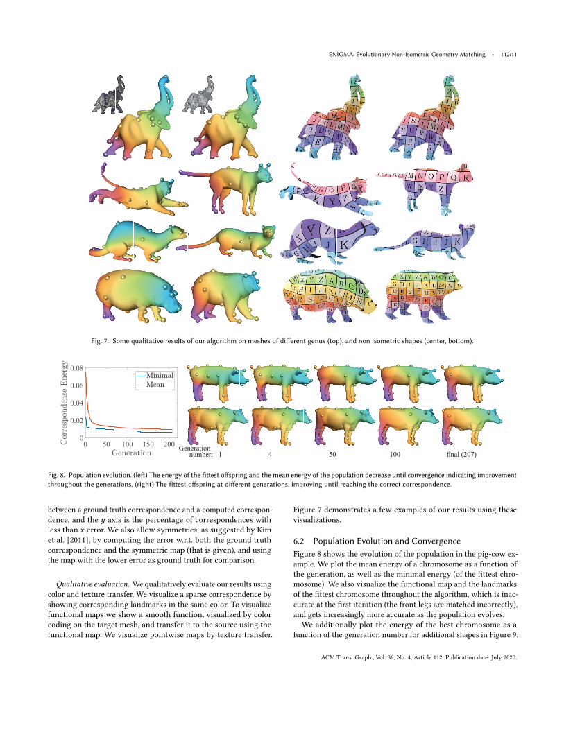
Fig. 7. Some qualitative results of our algorithm on meshes of different genus (top), and non isometric shapes (center, bottom).

0 50 100 150 2000

0.02

0.04

0.06

0.08

Fig. 8. Population evolution. (left) The energy of the fittest offspring and the mean energy of the population decrease until convergence indicating improvementthroughout the generations. (right) The fittest offspring at different generations, improving until reaching the correct correspondence.

between a ground truth correspondence and a computed correspon-dence, and the y axis is the percentage of correspondences withless than x error. We also allow symmetries, as suggested by Kimet al. [2011], by computing the error w.r.t. both the ground truthcorrespondence and the symmetric map (that is given), and usingthe map with the lower error as ground truth for comparison.

Qualitative evaluation. We qualitatively evaluate our results usingcolor and texture transfer. We visualize a sparse correspondence byshowing corresponding landmarks in the same color. To visualizefunctional maps we show a smooth function, visualized by colorcoding on the target mesh, and transfer it to the source using thefunctional map. We visualize pointwise maps by texture transfer.

Figure 7 demonstrates a few examples of our results using thesevisualizations.

6.2 Population Evolution and ConvergenceFigure 8 shows the evolution of the population in the pig-cow ex-ample. We plot the mean energy of a chromosome as a function ofthe generation, as well as the minimal energy (of the fittest chro-mosome). We also visualize the functional map and the landmarksof the fittest chromosome throughout the algorithm, which is inac-curate at the first iteration (the front legs are matched incorrectly),and gets increasingly more accurate as the population evolves.We additionally plot the energy of the best chromosome as a

function of the generation number for additional shapes in Figure 9.



Similarly to the pig-cow example, the energy decreases until thealgorithm converges.

0 0.05 0.1 0.15 0.2 0.250

20

40

60

80

100

TotalBes tWors t

Since our algorithm isnot deterministic, we in-vestigate the variation ofour results by runningthe algorithm 100 timeson 20 random pairs ofshapes from the SHREC’07dataset [Giorgi et al. 2007].We evaluate the result using the protocol suggested by Kim etal. [2011], after post processing [Ezuz et al. 2019b] to extract adense map. The results are determined by the total geodesic errorwith respect to the sparse ground truth and are shown in the insetFigure. The best and worst results are composed of the best andworst results of each one of the 20 pairs respectively. Note that thetotal results (all 100 results on all the pairs) are close to the bestresults, indicating that the worst results are outliers.

6.3 Mapping between Shapes of Different GenusOur method is applicable to shapes of any genus, and can also matchbetween shapes of different topology. Figure 1 shows our results fortwo hand models from SHREC’19 [Dyke et al. 2019]. The left modelhas genus 2 and the right model has genus 1. Note that our approachyields a high quality dense correspondence even for such difficultcases. We additionally show in Figure 10 our results for two cupmodels from SHREC’07 [Giorgi et al. 2007], both genus 1, and twopairs of human shapes with genus 0 and genus 1, respectively. Hereas well, despite the difficult topological issues, our approach com-puted a meaningful map. Another example appears in Figure 7 (top).Here, we generated a genus 8 mesh (left) by introducing tunnelsthrough a genus 3 mesh (right). Both meshes were then remeshed tohave different triangulations. Note that even for meshes with largedifferences in genus, our method generates good results.

0 100 200 3000

0.01

0.02

0.03

Fig. 9. The correspondence energy of the fittest offspring during the itera-tions (left) and the final map generated from the fittest offspring in the finaliteration (right) on a few pairs of shapes. Note that the energy decreasesuntil convergence.

Fig. 10. Our results on shapes of genus 1 (top) and shapes with differentgenus (bottom).

(a) (d)

(c)

(b)

(f)

(e)

Fig. 11. Varying degrees of isometry, from nearly isometric (a) to highlynon isometric shapes (f). Our method finds the correct map for most pairs(a-e), yet matches incorrectly the pair with the highest distortion (f).

6.4 Evaluation on increasingly non-isometric shapes.To demonstrate the efficiency of our algorithm on non-isometricshapes, we perform the following experiment. Starting from nearlyisometric shapes from the SHREC’07 dataset [Giorgi et al. 2007],we deform one of the shapes (extend the bears’ arm) graduallyand obtain 5 pairs with different degrees of isometric distortion(Figure 11). For the first 5 pairs (a-e) we find the correct matchdespite the large deformation, whereas for the last pair (f), wherethe non-isometric deformation is very high, our algorithm does notfind a correct map.

6.5 Ablation study.

0 0.05 0.1 0.15 0.2 0.250

20

40

60

80

100

Harmonic EnergyWithout CentersRandom initCX CrossoverWithout ShrinkageOur GA

We perform an ablationstudy to show the ef-fect of different designchoices of our algorithm.We run our algorithm5 times on 20 randompairs from the SHREC’07dataset [Giorgi et al. 2007],where each time one partof the method changeswhile the rest remainsidentical. In our first experiment, we use only the maxima andminima as landmarks, removing the centers. Next, we use a randompopulation initialization [Paul et al. 2013], change the fitness to the



0 0.05 0.1 0.15 0.2 0.250

20

40

60

80

100

BCICP [Ren18]BCICP [Ren18] +RHM [Ezuz19b]Tight relaxation [Kezurer15]DS++ [Dym17]GA+AS [Sahillioglu18]Ours

Fig. 12. Quantitative comparison between our results and fully automaticstate of the art methods [Dym et al. 2017; Kezurer et al. 2015; Ren et al. 2018;Sahillioğlu 2018]. We apply the same post processing [Ezuz et al. 2019b] onall the methods to extract a dense map, and use the evaluation protocolsuggested by Kim et al. [2011], that measures geodesic distance to theground truth. Note that we outperform all the other methods.

reversible harmonic energy [Ezuz et al. 2019b] of the functional mapextracted from a chromosome, use the cycle crossover (CX) from thetraveling salesman problem [Oliver et al. 1987], and finally removethe shrinkage mutation. We evaluate the results as in the previoussections and they are shown in the inset Figure. Note that changingparts of the algorithm diminishes the performance.

6.6 Quantitative andQualitative ComparisonsWe compare our method with state of the art methods for sparse anddense correspondence. We only compare with fully automatic meth-ods, since semi automatic methods require additional user input,which is often not available. For comparisons that require a densecorrespondence we apply the same post processing for all methods:we compute a functional map as described in section 5.3 and use itas input to the sparse-to-dense post processing method [Ezuz et al.2019b]. We compare the resulting dense pointwise maps quantita-tively using the protocol suggested by Kim et al. [2011] as describedin section 6.1.

The sparse correspondence methods we compare with are: "TightRelaxation" by Kezurer et al. [2015], DS++ by Dym et al. [2017], andthe recent method by Sahillioglu et al. [2018] that also uses a geneticalgorithm (GA+AS, AS stands for Adaptive Sampling which theyuse for improved results). We additionally compare with the recentdense correspondence method by Ren et al. [2018] (BCICP). SinceRen et al. [2018] computes vertex-to-vertex maps, we apply the postprocessing [Ezuz et al. 2019b] on their results as well (BCICP+RHM).

The quantitative results are shown in Figure 12, and it is evidentthat our method outperforms all previous approaches on this highlychallenging non-isometric dataset. The sparse correspondence andthe functional map are visualized in Figure 13 using the visualizationapproach described in Section 6.1. Note that our method consistentlyyields semantic correspondences on shapes from various classes,even in highly non-isometric cases such as the airplanes, the fish and

the dog/wolf pair. This is even more evident when examining thetexture transfer results in Figure 14, which visualize the dense map.Note the high quality dense map obtained for highly non-isometricmeshes such as the fish and the wolf/dog.We additionally compare our results to those of "Tight Relax-

ation" [Kezurer et al. 2015] when matching the same initial land-marks. We generate 15 landmarks for each shape, following themethod used in [Kezurer et al. 2015]. As this approach requires thematch size as an additional input, we use the values: 11, 13 as wellas the match size found automatically by our method as inputs. Theresults are shown in Figure 15. Note that the match found by ourmethod is correct and outperforms the competing output, whosequality also depends on the requested match size.

7 CONCLUSIONWe present an approach for automatically computing a correspon-dence between non-isometric shapes of the same semantic class. Weleverage a genetic algorithm for the combinatorial optimization ofa small set of automatically computed landmarks, and use a fitnessenergy that is based on extending the sparse landmarks to a func-tional map. As a result, we achieve high quality dense maps, thatoutperform existing state-of-the-art automatic methods, and cansuccessfully handle challenging cases where the source and targethave a different topology.We believe that our approach can be generalized in a few ways.

First, the decomposition of the automatic mapping computationproblem into combinatorial and continuous problems mirrors othertasks in geometry processing which were handled in a similar man-ner, such as quadrangular remeshing. It is interesting to investigatewhether additional analogues exist between these seemingly unre-lated problems. Furthermore, it is intriguing to consider what otherproblems in shape analysis can benefit from genetic algorithms.One potential example is map synchronization for map collections,where the choice of cycles to synchronize is also combinatorial.

ACKNOWLEDGMENTSThe authors acknowledge the support of the German-Israeli Foun-dation for Scientific Research and Development (grant number I-1339-407.6/2016), the Israel Science Foundation (grant No. 504/16),and the European Research Council (ERC starting grant no. 714776OPREP).We also thank SHREC’07, SHREC’19, AIM@SHAPE, RobertW. Sumner and Windows 3D library for providing the models.

REFERENCESNoam Aigerman and Yaron Lipman. 2015. Orbifold Tutte Embeddings. ACM TOG 34

(2015).Noam Aigerman and Yaron Lipman. 2016. Hyperbolic Orbifold Tutte Embeddings.

ACM TOG 35 (2016).Noam Aigerman, Roi Poranne, and Yaron Lipman. 2015. Seamless surface mappings.

ACM TOG 34, 4 (2015), 72.Mathieu Aubry, Ulrich Schlickewei, and Daniel Cremers. 2011. The Wave Kernel

Signature: A Quantum Mechanical Approach to Shape Analysis. In InternationalConference on Computer Vision Workshops (ICCV Workshops). IEEE.

Surapong Auwatanamongkol. 2007. Inexact graph matching using a genetic algorithmfor image recognition. Pattern Recognition Letters 28, 12 (2007), 1428–1437.

Thomas Back. 1996. Evolutionary algorithms in theory and practice: evolution strategies,evolutionary programming, genetic algorithms. Oxford university press.

Bir Bhanu, Sungkee Lee, and John Ming. 1995. Adaptive image segmentation usinga genetic algorithm. IEEE Trans on systems, man, and cybernetics 25, 12 (1995),1543–1567.



Tight Relaxation [Kezurer15] DS++ [Dym17] GA+AS [Sahillioglu] Ours

Fig. 13. Qualitative comparison between the results of our genetic algorithm, i.e. a sparse correspondence and a functional map, and the results of automaticstate of the art methods [Dym et al. 2017; Kezurer et al. 2015; Sahillioğlu 2018] for sparse correspondence. The functional map is visualized by color transfer(see text for details), and the sparse correspondence is visualized by landmarks with corresponding colors.

Davide Boscaini, Jonathan Masci, Emanuele Rodolà, and Michael Bronstein. 2016.Learning shape correspondence with anisotropic convolutional neural networks. InAdvances in Neural Information Processing Systems. 3189–3197.

Mario Botsch, Mark Pauly, Markus H Gross, and Leif Kobbelt. 2006. PriMo: coupledprisms for intuitive surface modeling. In Proc. Eurographics SGP. 11–20.

Alexandru Horia Brie and Philippe Morignot. 2005. Genetic Planning Using VariableLength Chromosomes.. In ICAPS. 320–329.

Xiuyuan Cheng, Gal Mishne, and Stefan Steinerberger. 2018. The geometry of nodalsets and outlier detection. Journal of Number Theory 185 (2018), 48–64.

Chi Kin Chow, Hung Tat Tsui, and Tong Lee. 2004. Surface registration using a dynamicgenetic algorithm. Pattern recognition 37, 1 (2004), 105–117.

Andrew DJ Cross, Richard C Wilson, and Edwin R Hancock. 1997. Inexact graphmatching using genetic search. Pattern Recognition 30, 6 (1997), 953–970.

Maya de Buhan, Charles Dapogny, Pascal Frey, and Chiara Nardoni. 2016. An optimiza-tion method for elastic shape matching. C. R. Math. Acad. Sci. Paris 354, 8 (2016),783–787.

Roberto Dyke, Caleb Stride, Yu-Kun Lai, and Paul L. Rosin. 2019. SHREC 2019. https://shrec19.cs.cf.ac.uk/.

Nadav Dym, Haggai Maron, and Yaron Lipman. 2017. DS++: A Flexible, Scalable andProvably Tight Relaxation for Matching Problems. ACM TOG 36, 6 (2017).

Davide Eynard, Emanuele Rodola, Klaus Glashoff, and Michael M Bronstein. 2016.Coupled functional maps. In 2016 Fourth 3DV. IEEE, 399–407.


https://shrec19.cs.cf.ac.uk/

https://shrec19.cs.cf.ac.uk/


Target Tight Relaxation [Kezurer15]

DS++ [Dym17] GA+AS [Sahillioglu18] BCICP [Ren18] + RHM [Ezuz19b]

Ours

Fig. 14. Qualitative comparison between our final results and fully automatic state of the art methods [Dym et al. 2017; Kezurer et al. 2015; Ren et al. 2018;Sahillioğlu 2018] (after applying the same post processing [Ezuz et al. 2019b] on all the methods to extract a dense map). The pointwise maps are visualizedusing texture that is computed on the target mesh (left) and transferred to the source using each method.

Danielle Ezuz and Mirela Ben-Chen. 2017. Deblurring and denoising of maps betweenshapes. In CGF, Vol. 36. Wiley Online Library, 165–174.

Danielle Ezuz, Behrend Heeren, Omri Azencot, Martin Rumpf, and Mirela Ben-Chen.2019a. Elastic Correspondence between Triangle Meshes. In CGF, Vol. 38.

Danielle Ezuz, Justin Solomon, and Mirela Ben-Chen. 2019b. Reversible Harmonic Mapsbetween Discrete Surfaces. ACM Transactions on Graphics (2019).

Danielle Ezuz, Justin Solomon, Vladimir G Kim, and Mirela Ben-Chen. 2017. Gwcnn: Ametric alignment layer for deep shape analysis. In CGF, Vol. 36. 49–57.

Anne Gehre, M Bronstein, Leif Kobbelt, and Justin Solomon. 2018. Interactive curveconstrained functional maps. In CGF, Vol. 37. Wiley Online Library, 1–12.

Daniela Giorgi, Silvia Biasotti, and Laura Paraboschi. 2007. SHREC: Shape RetrievalContest: Watertight Models Track.

Oshri Halimi, Or Litany, Emanuele Rodola, Alex M Bronstein, and Ron Kimmel. 2019.Unsupervised learning of dense shape correspondence. In Proceedings of the IEEEConference on Computer Vision and Pattern Recognition. 4370–4379.

Behrend Heeren, Martin Rumpf, Peter Schröder, Max Wardetzky, and Benedikt Wirth.2014. Exploring the Geometry of the Space of Shells. CGF 33, 5 (2014), 247–256.

Behrend Heeren, Martin Rumpf, Max Wardetzky, and Benedikt Wirth. 2012. Time-Discrete Geodesics in the Space of Shells. CGF 31, 5 (2012), 1755–1764.

John H Holland. 1992. Genetic algorithms. Scientific american 267, 1 (1992), 66–73.Haibin Huang, Evangelos Kalogerakis, Siddhartha Chaudhuri, Duygu Ceylan,

Vladimir G Kim, and Ersin Yumer. 2017. Learning local shape descriptors from partcorrespondences with multiview convolutional networks. ACM TOG 37, 1 (2017),1–14.

Ruqi Huang andMaks Ovsjanikov. 2017. AdjointMap Representation for Shape Analysisand Matching. In Computer Graphics Forum, Vol. 36. 151–163.

José A. Iglesias, Martin Rumpf, and Otmar Scherzer. 2018. Shape-Aware Matching ofImplicit Surfaces Based on Thin Shell Energies. Found. Comput. Math. 18, 4 (2018),891–927.

Itay Kezurer, Shahar Z Kovalsky, Ronen Basri, and Yaron Lipman. 2015. Tight relaxationof quadratic matching. In Computer Graphics Forum, Vol. 34. 115–128.

Vladimir G Kim, Yaron Lipman, and Thomas Funkhouser. 2011. Blended Intrinsic Maps.ACM TOG 30 (2011).

Isaak Lim, Alexander Dielen, Marcel Campen, and Leif Kobbelt. 2018. A simple approachto intrinsic correspondence learning on unstructured 3d meshes. In Proceedings ofthe European Conference on Computer Vision (ECCV). 0–0.

Or Litany, Tal Remez, Emanuele Rodolà, Alex Bronstein, and Michael Bronstein. 2017.Deep functional maps: Structured prediction for dense shape correspondence. InProceedings of the IEEE International Conference on Computer Vision. 5659–5667.

Nathan Litke, Mark Droske, Martin Rumpf, and Peter Schröder. 2005. An ImageProcessing Approach to Surface Matching. In Proc. Eurographics SGP. 207–216.

Roee Litman and Alexander Bronstein. 2014. Learning spectral descriptors for de-formable shape correspondence. Pattern Analysis and Machine Intelligence, IEEETransactions on 36, 1 (2014), 171–180.

Manish Mandad, David Cohen-Steiner, Leif Kobbelt, Pierre Alliez, and Mathieu Desbrun.2017. Variance-Minimizing Transport Plans for Inter-surface Mapping. ACM TOG36 (2017), 14.



Tight Relaxation [Kezurer15]

11 landmarks 13 landmarks

Ours

9 landmarksndm

9 landmarks

11 landmarks

10 landmarksSame amount of landmarks as ours

Fig. 15. Qualitative comparison with Tight Relaxation (TR) [Kezurer et al.2015] using the same 15 landmarks. (right) Our results, (three left columns)TR results with varying match size: 11, 13 and the size our method found.

Haggai Maron, Nadav Dym, Itay Kezurer, Shahar Kovalsky, and Yaron Lipman. 2016.Point Registration via Efficient Convex Relaxation. ACM TOG 35, 4 (2016).

Jonathan Masci, Davide Boscaini, Michael Bronstein, and Pierre Vandergheynst. 2015.Geodesic convolutional neural networks on riemannian manifolds. In The IEEEInternational Conference on Computer Vision (ICCV). 37–45.

Ujjwal Maulik and Sanghamitra Bandyopadhyay. 2000. Genetic algorithm-based clus-tering technique. Pattern recognition 33, 9 (2000), 1455–1465.

Federico Monti, Davide Boscaini, Jonathan Masci, Emanuele Rodola, Jan Svoboda, andMichael M Bronstein. 2017. Geometric deep learning on graphs and manifolds usingmixture model cnns. In Proceedings of the IEEE Conference on Computer Vision andPattern Recognition. 5115–5124.

Brent C Munsell, Pahal Dalal, and Song Wang. 2008. Evaluating shape correspondencefor statistical shape analysis: A benchmark study. IEEE Transactions on PatternAnalysis and Machine Intelligence 30, 11 (2008), 2023–2039.

Dorian Nogneng and Maks Ovsjanikov. 2017. Informative descriptor preservation viacommutativity for shape matching. In Computer Graphics Forum, Vol. 36. 259–267.

IM Oliver, DJd Smith, and John RC Holland. 1987. Study of permutation crossover oper-ators on the traveling salesman problem. In Genetic algorithms and their applications:proceedings of the second International Conference on Genetic Algorithms: July 28-31,1987 at the Massachusetts Institute of Technology, Cambridge, MA. Hillsdale, NJ: L.Erlhaum Associates, 1987.

Maks Ovsjanikov, Mirela Ben-Chen, Justin Solomon, Adrian Butscher, and LeonidasGuibas. 2012. Functional maps: a flexible representation of maps between shapes.ACM TOG 31, 4 (2012).

Maks Ovsjanikov, Etienne Corman, Michael Bronstein, Emanuele Rodolà, Mirela Ben-Chen, Leonidas Guibas, Frederic Chazal, and Alex Bronstein. 2016. Computing andprocessing correspondences with functional maps. In SIGGRAPH ASIA 2016 Courses.ACM, 9.

Ender Ozcan and Chilukuri K Mohan. 1997. Partial shape matching using geneticalgorithms. Pattern Recognition Letters 18, 10 (1997), 987–992.

Daniele Panozzo, Ilya Baran, OlgaDiamanti, andOlga Sorkine-Hornung. 2013. Weightedaverages on surfaces. ACM TOG 32, 4 (2013), 60.

P Victer Paul, A Ramalingam, R Baskaran, P Dhavachelvan, K Vivekanandan, R Subra-manian, and VSK Venkatachalapathy. 2013. Performance analyses on populationseeding techniques for genetic algorithms. International Journal of Engineering andTechnology (IJET) 5, 3 (2013), 2993–3000.

Adrien Poulenard and Maks Ovsjanikov. 2018. Multi-directional geodesic neural net-works via equivariant convolution. ACM TOG 37, 6 (2018), 1–14.

Jing Ren, Adrien Poulenard, Peter Wonka, and Maks Ovsjanikov. 2018. Continuousand Orientation-preserving Correspondences via Functional Maps. ACM TOG 37, 6(2018).

Jean-Michel Roufosse, Abhishek Sharma, and Maks Ovsjanikov. 2019. Unsuperviseddeep learning for structured shape matching. In Proceedings of the IEEE InternationalConference on Computer Vision. 1617–1627.

STANLEY GOTSHALL BART Rylander and S Gotshall. 2002. Optimal population sizeand the genetic algorithm. Population 100, 400 (2002), 900.

Yusuf Sahillioğlu. 2018. A Genetic Isometric Shape Correspondence Algorithm withAdaptive Sampling. ACM Trans. Graph. 37, 5 (Oct. 2018).

Luciano Silva, Olga Regina Pereira Bellon, and Kim L Boyer. 2005. Precision rangeimage registration using a robust surface interpenetration measure and enhancedgenetic algorithms. IEEE transactions on pattern analysis and machine intelligence27, 5 (2005), 762–776.

Justin Solomon, Gabriel Peyré, Vladimir G Kim, and Suvrit Sra. 2016. Entropic metricalignment for correspondence problems. ACM TOG 35, 4 (2016), 72.

Olga Sorkine and Marc Alexa. 2007. As-Rigid-As-Possible Surface Modeling. In Proc.Eurographics Symposium on Geometry Processing. 109–116.

Robert W Sumner and Jovan Popović. 2004. Deformation Transfer for Triangle Meshes.ACM TOG 23 (2004).

Gary KL Tam, Zhi-Quan Cheng, Yu-Kun Lai, Frank C Langbein, Yonghuai Liu, DavidMarshall, Ralph R Martin, Xian-Fang Sun, and Paul L Rosin. 2013. Registration of3D point clouds and meshes: a survey from rigid to nonrigid. IEEE Transactions onVisualization and Computer Graphics 19, 7 (2013), 1199–1217.

Ron Unger and John Moult. 1993. Genetic algorithms for protein folding simulations.Journal of molecular biology 231, 1 (1993), 75–81.

Oliver Van Kaick, Hao Zhang, Ghassan Hamarneh, and Daniel Cohen-Or. 2011. Asurvey on shape correspondence. In Computer Graphics Forum, Vol. 30. 1681–1707.

Matthias Vestner, Roee Litman, Emanuele Rodola, Alex Bronstein, and Daniel Cremers.2017. Product Manifold Filter: Non-rigid Shape Correspondence via Kernel DensityEstimation in the Product Space. In 2017 IEEE CVPR. IEEE, 6681–6690.

Lingyu Wei, Qixing Huang, Duygu Ceylan, Etienne Vouga, and Hao Li. 2016. Densehuman body correspondences using convolutional networks. In Proceedings of theIEEE CVPR. 1544–1553.

Yingzi Wei, Yulan Hu, and Kanfeng Gu. 2007. Parallel search strategies for TSPs using agreedy genetic algorithm. In Third International Conference on Natural Computation(ICNC 2007), Vol. 3. IEEE, 786–790.

Thomas Windheuser, Ulrich Schlickewei, Frank R Schmidt, and Daniel Cremers. 2011.Geometrically consistent elastic matching of 3d shapes: A linear programmingsolution. In Proc. IEEE International Conference on Computer Vision. 2134–2141.

Sameh M Yamany, Mohamed N Ahmed, and Aly A Farag. 1999. A new genetic-basedtechnique for matching 3-D curves and surfaces. Pattern Recognition 32, 10 (1999),1817–1820.

Hao Zhang, Alla Sheffer, Daniel Cohen-Or, Quan Zhou, Oliver Van Kaick, and AndreaTagliasacchi. 2008. Deformation-driven shape correspondence. InComputer GraphicsForum, Vol. 27. Wiley Online Library, 1431–1439.

A PARAMETERSAll the parameters are unitless and fixed in all the experiments. We choose the valuesexperimentally, yet our results are not sensitive to these values. Many of the parametersare required by the genetic algorithm and the functional map computations, whichboth have standard practices.

Centers. To compute the landmarks classified as centers from Eq. (11), we useN = 30 eigenfunctions, as suggested by Cheng et al. [2018].

Filtering. We filter close landmarks according to the initial distance of dϵ = 0.08,where the distance is on the normalized shape. In addition, we set the maximal amountof landmarks to µ = 35. We observed that for a variety of shapes, 35 landmarks withthe specified minimal distance covered the shape features well and gave a large enoughsubset of matching landmarks for our fitness function.

Adjacent landmarks. We use the geodesic distance of dadj = 0.3 to define adjacentlandmarks. This distance is large enough to accommodate highly non-isometric shapesbut still allows to construct consistent chromosomes.

Gene bank. We set the WKS distance to ϵwks = 0.2.Match size. The minimal match size ismmin =

23mmax and the maximal match size

ismmax = min(m1,m2) wheremi is the number of landmarks on Mi .Population construction. The initial population has 400 chromosomes, following

experiments with varying population sizes and the guidelines by Rylander et al. [2002].Functional map optimization. To construct the functional map we use ks = 30, kt =

60 and α = 1, β = 100, which is standard practice for functional maps computations.Functional map fitness. For the elastic energy, we set γ = 5 · 10−4 similarly to Ezuz

et al. [2019a].Genetic operators. For the operators, we use the rates pcross= 0.75, pдrow= 0.05

pshr ink= 0.1, pFMдuid= 0.05. The crossover is the main operator, therefore its rateis much higher than the mutations, as is common for genetic algorithms.

Convergence. We stop the algorithm if the fittest chromosome remains unchangedfor 50 iterations or when a maximal iteration number of 700 iterations is reached.


ENIGMA: Evolutionary Non-Isometric Geometry MAtching - arXiv

Documents

Transcript of ENIGMA: Evolutionary Non-Isometric Geometry MAtching - arXiv