MATHEMATICS OF OPERATIONS RESEARCH

Vol. 32, No. 3, August 2007, pp. 563–578issn 0364-765X �eissn 1526-5471 �07 �3203 �0563

informs ®

doi 10.1287/moor.1070.0254©2007 INFORMS

The Demand-Matching Problem

F. B. ShepherdBell Laboratories, 600 Mountain Avenue, Murray Hill, New Jersey 07974,

bshep@bell-labs.com, http://cm.bell-labs.com/cm/ms/who/bshep/

A. VettaDepartment of Mathematics and Statistics, McGill University, Burnside Hall, 805 Sherbrooke W.,

Montreal, Quebec, Canada, vetta@math.mcgill.ca, http://www.math.mcgill.ca/˜vetta/

We examine formulations for the well-known b-matching problem in the presence of integer demands on the edges. A subsetM of edges is feasible if for each node v the total demand of edges in M incident to v is at most bv . We examine the systemof star inequalities for this problem. This system yields an exact linear description for b-matchings in bipartite graphs. For thedemand version, we show that the integrality gap for this system is at least 2.5 and at most 2.764. For general graphs, the gaplies between 3 and 3.264. We also describe a 3-approximation algorithm (2.5 for bipartite graphs) for the cardinality versionof the problem. A fully polynomial approximation scheme is also presented for the problem on a tree, thus generalisinga well-known result for the knapsack problem. Recently, the notion of demand matching has arisen in the design of Closnetwork switches.

Key words : b-matching; linear programming; integrality gap; approximation algorithmMSC2000 subject classification : Primary: 90C27; secondary: 90C05, 90C59, 68W25OR/MS subject classification : Primary: networks/graphs: matchings; secondary: programming: integer, algorithmsHistory : Received January 14, 2004; revised February 18, 2005, October 10, 2005, and April 20, 2006.

1. Introduction. A combinatorial maximum packing problem is determined by a ground set V , each elementu of which has an associated profit, denoted pu, and a collection � of feasible subsets of V . The objective isto find a feasible set F ∈� inducing a profit p�F ≡∑

u∈F pu of maximum value. Feasibility for such problemsis often determined by some set of resource capacities into which at most some bounded number of groundelements can be packed. For instance, in the b-matching problem on a graph, a subset M of its edges is feasibleif each node v is incident to at most bv edges of M . We are interested in understanding the relationship ofsuch base problems, where ground elements in effect have a unit size, to their demand version, where theelements each come with an integer demand value. For instance, in the case of b-matchings, each edge e couldbe additionally supplied with a demand de. A set M of edges is then feasible if for each node v the total demandof edges in M incident to v does not exceed the capacity bv. Naturally, this gives rise to a completely differentcollection of feasible sets.Analysis for such demand problems often requires new methods from those used for the base problem itself.

This is largely because the whole demand must be satisfied before its profit may be reaped. Such “all-or-nothing”constraints arise quite naturally in practice; bandwidth trading in communication networks is one such example.In this paper, our attention is restricted exclusively to the case of hard capacity constraints. The quintessentialstarting place for this study is the knapsack problem. Here an integrality gap of two for the standard linearprogramming (LP) formulation is well known. Multiple knapsack problems, where the set of packable itemsis the same for each knapsack, have also been studied from the perspective of providing good approximationalgorithms, see Chekuri and Khanna [6]. Our interest, however, lies in understanding how the structure of somebase combinatorial problem interacts with its demand version. The demand b-matching problem, for instance,can be viewed as having many parallel knapsacks, one associated with each node. Coupling of the constraintsonly arises due to each edge being in two different knapsacks.Theoretical work on the demand versions of combinatorial packing problems has been rather limited. We now

review some of this work. One well-studied case of the generalized assignment problem is where each task hasa size independent of its assignment. This problem is a special case of the demand-matching problem. To seethis, note that the base problem can be viewed as a bipartite b-matching problem with the following property.Every node v on one side of the bipartition has a common demand value (associated with its task) on each ofits incident edges, and its bv-value is set to be equal to this demand value. The generalized assignment problem,in full generality where sizes may vary for a fixed task, was studied by Shmoys and Tardos [24], even thoughtheir focus was on congestion minimization. In fact, some of our techniques and findings bear resemblance totheirs. Their results are revisited and used in Chekuri and Khanna [6], where the maximization form is studied.A demand version of network flows was studied by Cosares and Saniee (cf. the ring-loading problem of

Cosares and Saniee [9]) and by Kleinberg [17], who gave the first general and comprehensive study of the topic.

563

Shepherd and Vetta: The Demand-Matching Problem564 Mathematics of Operations Research 32(3), pp. 563–578, © 2007 INFORMS

In particular, Kleinberg introduced the term unsplittable flow and, relevant to the study in the present paper, hewas the first to examine the maximization form of these problems. One example is the study (Kleinberg [18]), ofthe maximum single-source unsplittable flow problem. Here, the base combinatorial problem is that of packingpaths into an edge-capacitated network. In the single-source setting, one is also given a source s and a collectionof terminals t1� t2� � � � � tk with demands d1�d2� � � � � dk, respectively. In addition, it is common to require ano-bottleneck condition so that each di is at most the minimum edge capacity in the network. The packingproblem is to satisfy the maximum number of the demands subject to the edge capacity constraints. This problemmay be viewed in the “demand” framework as follows. Let each s − ti path have the demand di. If we add asink node t and edges tit of capacity di, then the goal is to find a maximum packing of the weighted s− t flowpaths. This single-source problem has been further developed in Kolliopoulos and Stein [19], Dinitz et al. [10],and Skutella [25].Unsplittable flow with general sets of commodities has also been studied. For instance, in Kolliopoulos and

Stein [20], the first approximation algorithm for general capacitated maximum unsplittable flow is given. Specialclasses of graphs have also been examined. Various special cases of the problem of packing subpaths (withdemands) in an edge-capacitated path are studied in Farach and Liberatore [13], Bar-Noy et al. [1], and Calinescuet al. [3], although a constant factor approximation for the general problem first appeared in Chakrabarti et al. [4].This was improved and extended to a constant factor (48) approximation for the maximum profit unsplittableflow problem where the underlying graph is a tree (Chekuri et al. [7]). We mention that the maximum unsplittableflow problem on the tree, without the no-bottleneck assumption, also includes the demand-matching problem,in the case where the tree is a star. Namely, the demand-matching graph may be represented by demand edgesbetween the leaf nodes of the star, and the node capacities are simulated by the edge capacities in the tree.A traditional attack in solving general packing problems is to find a linear description for the convex hull of

incidence vectors of feasible sets. A normal starting point is to formulate an integer program based on somem×n 0�1 matrix A: max�p ·x� Ax≤ b� xi ∈ �0�1�� where any 0, 1 solution identifies a feasible set. For example,if G is bipartite, then its node-edge incidence matrix is totally unimodular. Hence, this matrix immediately yieldssuch a formulation for the b-matching problem (Hoffman and Kruskal [15]), whose relaxation has an integralitygap of one. The demand version of the original 0�1 packing problem is then: max�p · x� Adx≤ b� xi ∈ �0�1��,where Ad is obtained from A by multiplying each column i by the value di. In Kolliopoulos and Stein [20],a framework is developed for relating such demand-packing problems to 0�1 packing problems. They referto a column-restricted packing integer program as one arising from such a matrix with all nonzero entries inany column the same, and with each di ≤ bj for each i, j .

1 They show that bounds on the integrality gapfor column-restricted packing problems can be directly tied to bounds on the integrality gaps for general 0�1packing problems. The key proof method is called grouping and scaling, whose origin is in the earlier paperKolliopoulos and Stein [19]. In fact, it follows from their work that a bound of � on the integrality gap for afamily of 0�1 packing problems translates to an O�� gap for the demand versions of the same family. Thisis stated explicitly in Chekuri et al. [7] for 0�1 packing problems arising from an arbitrary fixed matrix A.Specifically, the following result is given, whose proof is implicit in the work of Kolliopoulos and Stein [20].Let A be a fixed 0�1 matrix and � be a given class of so-called closed objective functions � . If � is the worst0�1 integrality gap of a packing problem for A and objective w ∈� , for any integral right-hand side b, then theworst gap for any such demand version is at most 11�54�. Several refinements are stated in Chekuri et al. [7]for application to other problems, and in particular for giving a unified handling, and some improvements, ofresults in Calinescu et al. [3], Bar-Noy et al. [1], and Chakrabarti et al. [4]. The potential for applying groupingand scaling was missed in these papers.We largely ignore the congestion minimization form of all of these problems. Connections between the

congestion minimization and maximization problems seem not to be fully understood and are worth exploring.For multicommodity flow where the supply graph is a tree, for instance, the congestion problem is trivial.Finding a maximum routable (obeying capacities) subset of the commodities, however, is not. Even the case ofunit profits and demands requires a nontrivial analysis (Garg et al. [14]); as mentioned, a constant gap for thegeneral version is given in Chekuri et al. [7].We close by mentioning a link between demand matchings and the design of a class of communication

switches. The switch is modelled as a graph with a bipartition of its nodes I ∪O representing its input and outputports. In addition, the edges of the graph come with (fractional) weights representing traffic amounts between

1 We mention that without the latter no-bottleneck assumption, there are examples where demand versions have arbitrarily large integralitygaps even if the starting matrix is total unimodular; this is described, for instance, in Chakrabarti et al. [4] for the problem of packingsubpaths (with demands) into a capacitated path.

Shepherd and Vetta: The Demand-Matching ProblemMathematics of Operations Research 32(3), pp. 563–578, © 2007 INFORMS 565

corresponding ports. The goal is to schedule transmission of traffic for all edges, using a minimum number oftime slots. This amounts to colouring the edges, so that each colour class is a demand matching (where eachbv = 1). An introduction to this area and some of its open problems can be found in Ngo and Vu [21] and Duet al. [11]. They consider a model where each node of the bipartite graph has a maximum fractional degreeof . Moreover, they assume that at each node v, of fractional degree k, say, the edges incident to v can bepartitioned into k “bins,” each of whose fractional weight is one. The goal is to find a smallest constant c suchthat the edges can be partitioned into c demand matchings (asymptotically). The current best such bound on cis 2.548 (Correa and Goemans [8]); there a more general version is studied where the bin condition is weakenedand one only requires that the fractional weight of each edge is at most one. The best lower bound for the switchproblem is presently given by c= 5

4 . At first glance our integrality gap of 2.5 for demand matching in bipartitegraphs would seem to suggest a 2.5 lower bound for the above problems. However, our lower-bound examplesdo not satisfy the extra bin conditions from the switch design problem. In fact, the demands (weights) on ouredges are not even bounded by one. It is an interesting question to understand the colouring question when onewishes to partition into general demand matchings.

1.1. The demand-matching problem. Take a graph G= �V �E and let each node v ∈ V have an integralcapacity, denoted by bv. Let each edge e = uv ∈ E have an integral demand, denoted by de. In addition,associated with each edge e ∈ E is a profit, denoted by pe. A demand matching is a subset M ⊆ E such that∑

e∈#�v∩M de ≤ bv for each node v. Here #�v denotes the set of edges of G incident to v. We assume, throughout,that the demand of any edge is less than the capacities of both its endnodes; otherwise, such an edge is notcontained in any demand matching and may be discarded. The demand-matching problem is to find a demandmatching of maximum profit. It can be formulated as the following integer program.

max∑e∈Epeye

s.t.∑e∈#�v

ye de ≤ bv ∀v ∈ V �

ye ∈ �0�1� ∀ e ∈E�

(1)

We also associate with an edge e a value, %e = pe/de, which we call the marginal profit of that edge. Marginalprofits play an important role in the understanding of demand matchings and, as a result, it will be useful toreformulate the integer program (1) in terms of marginal profits. Doing so, we obtain the following integerprogram.

max∑e∈E%exe

s.t.∑e∈#�v

xe ≤ bv ∀v ∈ V �

xe ∈ �0�de� ∀ e ∈E�

(2)

There are several special cases of the demand-matching problem that are interesting in their own right. Webegin by considering specific demand and profit functions.

(i) Unit Demand Function: The demand of each edge is one. Observe that this problem is just the familiarb-matching problem. Hence, the unit demand version can be solved in polynomial time.(ii) Maximum Cardinality Demand-Matching Problem: The profit associated with each edge is one, and

hence the objective is to find a feasible demand matching containing as many edges as possible.(iii) Constant Marginal Profit Function: The profit associated with each edge is proportional to its demand.

As a result, the marginal profit of each edge is the same.Particular underlying graphs also give rise to interesting subproblems. For example, suppose that the under-

lying graph is a star, i.e., a tree in which every node is a leaf except for the root node r . In this case, thedemand-matching problem is equivalent to the knapsack problem, where the knapsack capacity is br and thereis an item of weight de for each edge e. In addition, if we have a unit marginal profit function, then thedemand-matching problem on a star includes the familiar subset-sum problem. As a consequence, we note thatthe demand-matching problem is NP-hard even where G is a star.

Shepherd and Vetta: The Demand-Matching Problem566 Mathematics of Operations Research 32(3), pp. 563–578, © 2007 INFORMS

1.2. An overview of the paper. The paper is organized as follows. In §2 we show that the demand-matchingproblem, even in the cardinality case, is MAXSNP complete. In §3 the natural linear programming relaxation isstudied. Here it is seen that the integrality gap for the formulation is at least 2 12 for bipartite graphs (whereas,it is 1 for the unit-demand case) and at least 3 for general graphs. We also discuss an extension of Berge’sAugmenting Path Theorem, which gives an optimality certificate for fractional demand matchings. Most of theremainder of the paper seeks upper bounds on the integrality gap of the linear program by way of approximationalgorithms that turn fractional solutions into integral solutions. The basic scheme uses augmenting paths and isintroduced in §4. It yields a 3-approximation for bipartite graphs and a 3 12 -approximation for general graphs. In§4.3 it is seen that understanding the integrality gap is related to determining the fractional chromatic numberof bipartite graphs where some of the edges have been subdivided. A randomised algorithm is then devisedfor this problem that improves the general bound for bipartite graphs to 2.764 (and 3.264 for general graphs).In §5 algorithms for the cardinality problem are presented, with approximation guarantees of 2 12 for bipartitegraphs and 3 for general graphs. Finally, in §6 we present a fully polynomial time approximation scheme forthe problem in which the underlying graph is a tree; this generalises the well-known result for the knapsackproblem (Ibarra and Kim [16]).

2. Hardness results. We have already seen that the demand-matching problem is hard for instances withunit marginal profit functions. However, we have also seen that instances with a unit demand function arepolynomially solvable. In this section, we examine the hardness of the demand-matching problem in moredetail. In particular, we show that the maximum cardinality demand-matching problem (and hence the generaldemand-matching problem) is MAXSNP-hard. Thus, there exists a constant ( > 0 such that the problem admitsno 1/�1− (-approximation algorithm unless P = NP . We say that 1/�1− ( is the inapproximability constantfor the problem.

Theorem 2.1. The cardinality demand-matching problem is MAXSNP-complete (even if the demands arerestricted to be one or three).

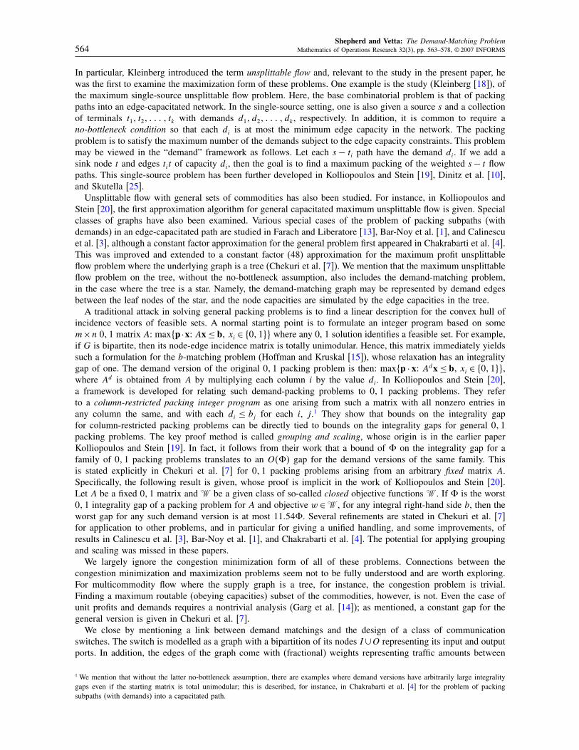
Proof. We first give a reduction from the the stable set problem to the cardinality demand-matching problem.Let �G�k be an instance of the (decision) stable set problem; that is, we want to know whether or not G containsa stable (pairwise nonadjacent) set of nodes of cardinality k. We construct an instance G′ of the (decision)cardinality demand-matching problem such that G has a stable set of size k if and only if G′ has a demandmatching of size 2m+ k, where m is the number of edges in G. For each node v in G we have two nodes vand v connected by an edge in G′. In addition, for each edge uv in G there is a node �u� v in G′. Betweennodes v and �u� v there is a path consisting of two edges. Similarly, there is a path consisting of two edgesbetween the nodes u and �u� v. Thus, for each node v in G we have an associated gadget in G′; such a gadgetis shown in Figure 1. Here v is adjacent to u1� u2� � � � � ur in G, where r equals the degree, dv, of v in G. Wesay that node v is selected by a demand matching if the matching contains all the dv+1 “outer” edges from v’sgadget (these outer edges are shown in bold in Figure 1). If the demand matching chooses the dv “inner” edgesfrom the gadget, then v is said to be deselected. If each node is either selected or deselected, then the size ofthe demand matching is

∑v�S d�v+

∑v∈S�d�v+ 1=

∑v d�v+ �S�, where S is the set of selected nodes.

(u1, v) (u2, v) (u3, v) (ur , v)

dv times

v

v dv

dv

dv

Figure 1. A gadget.

Shepherd and Vetta: The Demand-Matching ProblemMathematics of Operations Research 32(3), pp. 563–578, © 2007 INFORMS 567

To enforce these selection rules, we set the capacity of each node in a gadget to be one, with the exceptionof v and v, which have capacity dv. In addition, every edge has demand one, except for edges of the form vv,which have demand dv. This ensures that if vv is chosen, then none of the inner edges may be, and that onlyone of the two edges on the path from the node v to the node �u� v may be chosen. One sees that any demandmatching that contains d�v+ 1 edges from a node v’s gadget must use the edge vv. Moreover, take a demandmatching of size 2m+k, for some k. Such a matching can easily be transformed into a demand matching of thesame or greater magnitude, in which each node is either selected or deselected. By our choice of capacities, wethen have that the selected nodes form a stable set in G. Conversely, suppose S is a stable set of size k in G.Then the union of the outer edges from gadgets corresponding to nodes in S with the inner edges from gadgetscorresponding to nodes not in S gives a matching of cardinality 2m+ k. Thus, we have the desired reduction.We now complete the proof of MAXSNP completeness for the case of demands 1 and 4; similar arguments

apply if we restrict to demands 1 and 3. Consider the maximum stable set problem in graphs with boundedmaximum degree. Inapproximability results are given in Berman and Karpinski [2] for such graphs; for graphsof maximum degree 4 it is hard to find a stable set within a factor of 1.0136 (roughly) of the optimum. So,suppose we have an 1/�1−(-approximation for the cardinality demand-matching problem. Now take a graph Gof maximum degree 4 with a maximum stable set of size k. Observe that k ≥ n/5 ≥ m/10. In addition, ourreduction produces a graph G′ with maximum demand matching of cardinality opt = 2m+ k. Applying ourapproximation algorithm, we obtain a demand matching of cardinality at least �1−(�2m+k. This correspondsto a stable set in G of size at least �1− (�2m+ k− 2m= �1− (k− ( · 2m≥ �1− (k− ( · 20k= k�1− 21(.Therefore, 1/�1− 21( ≥ 1�0136, and hence the inapproximability constant for the demand-matching problemis at least 1.00064.It is straightforward to check that this approach also applies if we use cubic graphs, but a slightly weaker

inapproximability constant results. �

We close by mentioning that it is now independently known (Shepard and Wilfong [23], Woeginger [26])that the maximum demand-matching problem remains NP-hard in bipartite graphs, even when all demands arerestricted to be either one or two.

3. A linear programming relaxation. We now consider the linear program relaxation of the formulation (2),i.e., for each edge we now have the linear constraints 0 ≤ xe ≤ de. We call the solution space of the resultantlinear program the fractional demand-matching polytope. We say that a point x in the polytope is a fractionaldemand matching. We also call x basic if it is an extreme point of the polytope. In this section we investigatethe structure of this polytope and its extreme points; we apply the results later when we return to the integralproblem.

3.1. Lower bounds on the integrality gap. We first describe some lower bounds on the integrality gapof the linear programming relaxation. For trees the integrality gap is at least two (we will see in §4 that itis exactly two). This is well known because there is a class of knapsack problems for which the fractionaloptimum is twice the integral optimum. An example is shown in Figure 2a, where the nodes are labelled bytheir capacities. For nonbipartite graphs, we now show that the integrality gap of the linear program is at leastthree asymptotically. Consider the simple example shown in Figure 2b. Note that no node can satisfy bothof its incident edge demands. Thus, the optimal integral solution contains exactly one edge from the triangle.Because each edge has value pe = 1, the optimal integral solution has value one. However, consider setting eachedge weight to be xe = k− 1. This gives a feasible fractional demand matching with profit 3− 3/k. Thus, theintegrality gap is at least three. Finally, for bipartite graphs, Figure 3 shows that the integrality gap is at least 2 12 ,even for cardinality instances. The optimal integral solutions contain exactly two edges. However, the fractionalsolution, shown in Figure 3, gives a profit of value 5− 4/k− �k− 1/W , for some constants W and k. This is5− 5/k if we set W = k�k− 1, given that the claimed gap k becomes large.

kk

2k–1 2k–2

2k–22k–2

(pe, de, xe)

(1, k , k–1)(1, k, k)

(b)(a)

Figure 2. Lower-bound examples for trees and nonbipartite graphs.

Shepherd and Vetta: The Demand-Matching Problem568 Mathematics of Operations Research 32(3), pp. 563–578, © 2007 INFORMS

W+ k–1

W

2k–2

2k–22k–2

(pe, de, xe)

(1, k , k–1)(1, W, W–k +1)

Figure 3. A lower-bound example for bipartite graphs.

3.2. Basic solutions of the fractional demand-matching polytope. For a fractional demand matching x anode v is termed tight if

∑e∈#�v xe = bv; otherwise, the node is termed slack. We say that an edge e is tight if

xe = de; we say that e is fractional if 0< xe < de. Let F �x⊆ E be the set of fractional edges induced by thefractional demand matching x. Let G�x denote the graph induced by F �x.

Lemma 3.1. Let x be an extreme point of the demand-matching polytope. Then each component of G�xconsists of a tree plus (possibly) one edge. In addition, any cycle in G�x has odd length.

Proof. First, suppose that G�x contains an even cycle C = �e1� e2� � � � � e2k�. For any (, we define y bysetting yei = xei + �−1i( for each i = 1�2� � � � �2k and ye = xe for any other edge e. Similarly, we definez �= x − �y − x. Observe that, because the edges on the cycle are fractional, there exists a positive ( suchthat both y and z are feasible. We then obtain the contradiction that x = 1

2 �y + z. Next suppose that somecomponent contains two odd cycles C1 and C2. The cycles do not share an edge; otherwise, they induce an evencycle. Thus, C1 and C2 are edge disjoint and connected by a (possibly empty) path P . Observe that the edgeset C1 ∪ P ∪C2 ∪ P is an even-length circuit. We then obtain a contradiction by similar reasoning to that givenabove except that increments along P are by ±2(. The result follows. �

3.3. Berge conditions for fractional demand matchings. Berge’s classic result on matchings asserts thata matching is of maximum cardinality if and only if it has no augmenting path. This result does not have asimple generalization for demand matchings. We can, however, extend this result to give optimality conditionsfor the fractional demand-matching problem. We begin with some definitions. Suppose we partition some subsetof the edges into two sets � ∪� . We call the resultant edge sets the positive edge set and the negative edge set,respectively. The marginal value %�F of a set of edges F ⊆� ∪� is just the sum of the marginal values of itspositive edges minus the sum of the marginal values of its negative edges, i.e., %�F =∑

e∈F∩� %e−∑

e∈F∩� %e.A balloon is formed by an odd-length cycle attached to a (possibly empty) path known as the string. A dumbbellis formed by two edge-disjoint odd-length cycles connected by a (possibly empty) path known as the rod.A structure is either a path, an even-length cycle, a balloon, or a dumbbell.A path P is called augmenting (with respect to x) if there is a partition � ∪� of E such that (i) edges on

the path are alternately positive and negative (or vice versa); (ii) %�P > 0; (iii) if an endpoint v of the path istight, then its incident edge is negative; (iv) none of the positive edges in P is tight. The motivation behind thisdefinition is as follows. The first two conditions state that it is beneficial to augment around the structure, i.e.,add ( weight to the positive edges, remove ( weight from the negative edges. Such an augmentation maintainsfeasibility with respect to the node constraints at internal nodes in the path. The third condition ensures that, forsmall (, the node constraints remain satisfied at the endnodes as well. Finally, the fourth constraint ensures that,for small (, the edge constraints also remain satisfied. Thus, if we find an augmenting path we may improveour current demand matching.Other structures may also be augmenting. An even-length cycle is just a closed path of even-length, and a

dumbbell is an even-length circuit in which the edges in the rod are traversed twice. Thus, augmenting cycles(and dumbbells) can be defined analogously to augmenting paths. Here, however, we may omit condition (iii).This is because in an even circuit all the nodes may be considered internal to the path. Observe that a balloon isjust a closed odd-length path in which edges on the string are traversed twice. Thus, augmenting balloons canbe defined analogously to augmenting paths. Note that because the circuit is of odd length, some node, say v,is incident only to positive edges (or only to negative edges). We may think of v as the endpoint of the balloonand, thus, in defining augmenting balloons we do require condition (iii). It is also easy to see that it is beneficialto augment along any of these other augmenting structures.

Shepherd and Vetta: The Demand-Matching ProblemMathematics of Operations Research 32(3), pp. 563–578, © 2007 INFORMS 569

Theorem 3.1. A fractional demand matching is optimal if and only if it induces no augmenting structure.

Proof. We have seen that in the presence of an augmenting structure the fractional demand matching cannotbe optimal. To prove the other direction, take an optimal fractional demand matching x∗. Given that x induces noaugmenting structure, we show that x gives the same profit as x∗ and is therefore optimal. Towards this end, letG′ = x∗ ⊕ x denote the symmetric difference between x∗ and x. That is, the edge set of G′ is E ′ = �e� x∗e �= xe�.An edge e in E ′ is given a marginal value of %e. In addition, the edge set is divided into two classes M∗ and M ,where M∗ = �e ∈E ′� x∗e > xe� and M = �e ∈E ′� x∗e < xe�.Choose an arbitrary node v in G′. Grow a maximal alternating path in the obvious way (where edges are

alternately in M and M∗, or vice versa). If we discover an even-length cycle or a dumbbell, then stop. Similarly,stop if we obtain a balloon with a maximal length string, or if both ends of the path cannot be extended. Thus,we obtain a structure S because some structure must be present. Note that e ∈M∗ implies that 0≤ xe < x∗e ≤ 1.In particular, this implies that xe may be increased by ( and x

∗e may be decreased by (, for a small positive value

of (. Now e ∈M implies that 0≤ x∗e < xe ≤ 1 and similar comments apply. In addition, note that if an endnode vof the structure S is only incident to edges of M∗, then v is slack with respect to the fractional demand matchingx, and vice versa. These observations imply that we may augment with respect to x∗ in one direction along thestructure and augment with respect to x in the other direction (we slightly abuse the definition of augmentation,because one of these augmentations has a nonpositive marginal value).Consider the marginal value of this structure (where the edges in M∗ are positive and the edges in M are

negative). The structure is not augmenting with respect to x and so %�S≤ 0. However, %�S cannot be negative,otherwise an augmentation with respect to x∗ is beneficial, and hence x∗ is not optimal. Thus, %�S = 0, sox∗ and x give the same profit on the edges in S. We remove the edges in S from G′ and search for anotherstructure. It follows that x is optimal. �

4. Linear programming-based algorithms.

4.1. Transforming a fractional demand matching: The augmenting paths procedure. In this section,we present deterministic approximation algorithms for the demand-matching problem. At the heart of thesealgorithms is a procedure that takes a fractional demand matching on a tree and transforms it so as to reveala two colouring of the edges. Each colouring will induce a feasible demand matching, thus giving a factor 2approximation guarantee for the demand-matching problem on a tree. This procedure is then used as a subroutinein an algorithm that gives a factor 3 guarantee if the underlying graph is bipartite, and a factor 3 12 approximationguarantee in general graphs.As the algorithm for trees lies at the heart of the main algorithm, we tackle this specific case first. Take an

optimal solution x to the linear programming relaxation of (2) on a tree. We show how to obtain an integraldemand matching whose profit is at least half of that of the fractional demand matching x. To do this, we showthat T contains two disjoint integral demand matchings whose combined profit is at least that of x.The algorithm is as follows. We may assume that any edge e with xe = 0 has been discarded. Set t = 0

and let x = f0 + h0. Here f0 is the vector obtained by setting all edges not in F �x equal to zero, and h isthe vector obtained by setting all the nontight edges equal to zero. Whilst the forest F �f t does not form astandard 1-matching, take any tree T ′ in F �f t that is not a single edge and choose two leaves i and j . LetP = �e1� e2� � � � � ek� be the path in T ′ between i and j . For some small (, we define y by setting yei = f tei+�−1i(for each i = 1�2� � � � � k and ye = xe for any other edge e. Similarly, we define z �= f t − �y − f t. The profitassociated with either y or z is at least that of f t . Without loss of generality, we may assume that z is moreprofitable. We then set f t+1 = z. (Note that feasibility at one or both of the endnodes of the path may be violatedfor the new vector z. This will not be an issue for us, because we will ultimately partition the final result intotwo feasible demand matchings.) Clearly, we may choose ( so that either some edge becomes tight in f t+1 (inwhich case we remove the edge from f t+1 and add it to ht to obtain a new set of tight edges ht+1), or someedge becomes zero and it is discarded.We call the above process of modification of our linear programming solution the augmenting paths procedure.

By construction, the value of the solution improved at each step. Therefore, the solution f t∗ + ht

∗at the end of

the augmenting paths procedure has profit of at least that of the optimal fractional demand matching x. Becausean edge is removed from F �f t at each step, we terminate in �E� phases with a forest F �f t∗ that forms a1-matching.As previously remarked, at some stage, f t + ht may no longer be feasible. On any given path augmentation,

however, the node constraints at internal nodes in the path continue to hold. It is only nodes at the ends of

Shepherd and Vetta: The Demand-Matching Problem570 Mathematics of Operations Research 32(3), pp. 563–578, © 2007 INFORMS

such a path that may become infeasible. For any such node, after the augmentation, either it is still a leaf in thefractional subgraph, or the unique fractional edge incident to it becomes tight. In the latter case, this node willnever participate in any more augmentations. Motivated by this observation, we say that an edge e is bronzewith respect to v and some f t , if e ∈ #�v and either (i) e is in F �f t or (ii) v is not incident to an edge in F �f t,and e was the final edge incident to v to become tight. Otherwise, we say that e is a copper edge with respectto v. We call an edge bronze if it is bronze with respect to either of its endpoints, and call it copper otherwise.Note that a node v at termination of the procedure is incident to at most one edge that is bronze with respectto v. However, it may be incident to several edges that are copper with respect to v and yet are bronze withrespect to a neighbour of v.We show how to use the copper-bronze edge colouring to find two feasible demand matchings on the supports

of f t∗and ht

∗. This then immediately yields a factor 2 approximation algorithm. The following lemma will help

us towards this goal.

Lemma 4.1. The set of copper edges with respect to a node v are collectively feasible with regards to theassociated node constraint.

Proof. If there is no bronze edge with respect to v, then all of the incident edges were tight in the initiallinear program solution. Hence, they are all collectively feasible at v, so let b be a bronze edge with respectto v. Let the copper edges with respect to v, ordered according to the order in which they became tight, bec1� c2� � � � � ck. Consider the edge ci, and suppose it became tight whilst augmenting the path P . Note that theedge b must have been fractional at this time. Thus, v was not a leaf node in some fractional tree. Therefore, vwas an internal node on the path P and the associated node constraint remained satisfied after the augmentation.Thus, c1� c2� � � � � ci were collectively feasible with respect to the node constraint at v. �

The following theorem now shows that we have a factor 2 approximation algorithm for the case in which theunderlying graph is a tree. (This is substantially improved in §6.)

Theorem 4.1. A tree contains two disjoint demand matchings M1 and M2 whose combined profit is at leastthat of the optimal fractional demand matching.

Proof. Apply the above procedure to a basic optimal fractional demand matching. The edges in the treecan now be partitioned into two feasible demand matchings as follows. By Lemma 4.1, a node v’s capacityconstraint is violated by a set of edges only if the set contains v’s bronze edge plus at least one other edge of#�v. In order to partition into two feasible demand matchings, it is thus sufficient to two-colour the edges sothat the bronze edge with respect to any node v receives a different colour from all other edges of #�v. Such acolouring can be found greedily, starting from an arbitrary root node in the tree, and then working out towardsthe leaves. The combined profit of the resulting matchings is at least that of the optimal fractional demandmatching and, therefore, at least that of the optimal demand matching. �

Recall, by Lemma 3.1, that F �x is (almost) a forest for general graphs. This observation will allow us touse our algorithm for trees to obtain an approximation algorithm for general graphs. We first consider bipartitegraphs.

Theorem 4.2. There is a factor 3-approximation algorithm for the demand-matching problem on bipartitegraphs.

Proof. Solve the linear programming relaxation to get a basic optimal solution. If the tight edges in thelinear program provide at least one-third of the profit of the optimal fractional solution (i.e., the value of thelinear program), then we are done. Otherwise, the fractional edges provide two-thirds of the total profit. Becausethe graph is bipartite, by Lemma 3.1 the fractional edges form a tree. Thus, we can find an integral demandmatching in the tree with at least half the value of the optimal fractional solution on that tree. This integraldemand matching has, therefore, value of at least one-third that of the LP. �

We may now consider nonbipartite graphs. We will need the following lemma.

Lemma 4.2. Let x be a basic optimal demand matching and let C be an odd cycle in F �x. Then C eithercontains an edge e with xe ≤ 1

2de or an edge e such that the set of tight edges in x plus e form a feasibledemand matching.

Proof. Take any odd cycle C induced by the fractional edges of x. Let e be the edge in C for which de−xeis minimized. Let e be incident to e1 and e2 on this cycle. Observe that if de − xe ≤min�xe1� xe2, then the setof tight edges still form a feasible demand matching even with the addition of e as desired. Otherwise, supposede− xe > xe1 , say. Then, because de− xe ≤ de1 − xe1 , we have that xe1 ≤ 1

2de1 . �

Shepherd and Vetta: The Demand-Matching ProblemMathematics of Operations Research 32(3), pp. 563–578, © 2007 INFORMS 571

Theorem 4.3. There is a factor 312 -approximation algorithm for the demand-matching problem on nonbi-partite graphs.

Proof. We again begin by partitioning the edge set induced by x into fractional edges and tight edges. Wewould like fractional edges to induce two demand matchings as before. However, we may not be able to do thisbecause the fractional edges may, by Lemma 3.1, induce components that contain a single odd cycle. Instead,we obtain a total of four demand matchings by the following method.Because the odd cycles in F �x are node disjoint, we may apply Lemma 4.2 to remove one edge from each

odd cycle. We either add each such edge to a new set S of edges with property xe ≤ 12de, or to the set of

tight edges. Again, because the odd cycles are node disjoint, the set S induces a matching, and hence inducesa demand matching. The set of tight edges (plus any edges added during this process) also form a feasibledemand matching. Finally, the remaining set of fractional edges induces a forest, from which we may obtaintwo demand matchings. Thus, we have partitioned the support of x into four demand matchings. Moreover, theedges in S have twice the profit that they contributed to the profit of x. It follows that one of these demandmatchings induces a profit of at least 2

7 that of the linear programming solution. �

4.2. Augmenting path procedure in general graphs: Extending the edge colouring. The method of §4.1produces a bronze-copper colouring of the fractional edges of the linear program solution (except for thoseedges that get discarded during the augmenting paths procedure). It will be useful in the following sections ifwe extend this edge colouring to include all the edges in the linear program solution. In particular, we willgenerate a 2-colouring of the edges for bipartite graphs, and a 3-colouring for nonbipartite graphs. Take a basicoptimal fractional demand-matching x. Note that x induces a set of tight edges and a fractional subgraph. Eachfractional component is a tree, together (possibly) with an extra edge that induces an odd cycle. All of thetight edges induced by x are also termed copper with respect to both of their endpoints. The fractional edgesare coloured bronze, copper, and red by the following augmenting paths procedure. We again augment alongleaf-to-leaf fractional paths, with the additional possibility that augments may be from a leaf to itself, via theodd cycle. Note that nonsimple augmentations use increments of size ±2( along the stem of the augmentingpath, whereas along the odd cycle the increments are ±(. As before, we choose the direction of the swaps so asto improve the profit of the fractional demand matching. In addition, we do not alter feasibility at a node unlessit was the leaf of the augment.Note that at some point in the process a fractional component may contain no leaves, i.e., it is an odd cycle.

If some edge e on the cycle has the property that xe ≤ 12de, then we colour e red and remove it from the

component. We then continue the augmentation procedure and colour the rest of the edges copper or bronze. Ifno edge has this property, then by Lemma 4.2 there is an edge e with the property that de− xe ≤min�xe1� xe2,where e is incident to e1 and e2 on the cycle. We colour e copper with respect to both its endpoints, remove itfrom the component, and continue the augmentation procedure. Note that e1, e2 are now leaves in the fractionalgraph, and hence will eventually either be dropped from the solution or be coloured bronze. The procedureterminates when the set of fractional edges forms a matching and all the edges are coloured. Note also that thered edges form a matching. Based on the remarks above, it is easy to check that Lemma 4.1 still holds, evenwith respect to the enlarged set of copper edges generated by this extended colouring. This observation will beneeded in the subsequent sections.

4.3. To stable sets and a randomised algorithm. In this section we show that the case of bipartite graphsis qualitatively different from the case of nonbipartite graphs with respect to the linear programming relaxation.In particular, we show that the integrality gap of the linear program is strictly less than three for bipartite graphs.This we achieve via the use of a randomised algorithm. Before presenting the randomised algorithm, we firstshow how the edge colouring induced by the linear program allows us to recast our problem as a stable setproblem. Consider first that we are in the bipartite case; hence, all the edges are coloured bronze or copper (forthe nonbipartite case it will actually suffice to just remove the red edges).Our stable set problem will be on a subgraph G′ of the line graph induced by G. The nodes of G′ are the

bronze and copper edges of G; for simplicity, we also call the nodes in G′ bronze and copper. The decision ofwhether to include an arc from the line graph in G′ is based on the copper and bronze edge interactions; forclarity, we refer to arcs in G′ and edges in G. Two nodes induce an arc in G′ if their corresponding edges in Gshare an endpoint v and one of the edges is bronze with respect to v.If we think of orienting bronze edges in G towards each node for which they are bronze, then we obtain a

digraph of maximum in-degree one. Moreover, any cycle would be of length two. It follows that the bronze

Shepherd and Vetta: The Demand-Matching Problem572 Mathematics of Operations Research 32(3), pp. 563–578, © 2007 INFORMS

nodes in G′ induce a forest. The copper edges induce nodes of degree of at most two in G′, because for acopper edge uv it may be incident to at most one bronze edge incident to u and one to v. Note that it may notbe possible to place uv in a demand matching with either of the bronze edges with respect to u and v. We avoidsuch conflicts if we restrict to edge sets of G corresponding to stable sets in G′. Indeed, it follows from Lemma4.1 that a stable set in G′ corresponds to a demand matching in G.We now present a randomised algorithm for the general demand-matching problem in bipartite graphs. The

algorithm gives an improved approximation guarantee of 2.764 for bipartite graphs. We work on the inducedstable set problem in the associated graph G′. The randomised algorithm first selects a stable set from amongstthe bronze nodes. It then greedily adds any copper node for which no bronze neighbour is in the stable set.The algorithm works as follows. Take the forest induced by the bronze nodes. For each tree in the forest, pickan arbitrary root node r . We now give the nodes in the tree a 0, 1 labelling. First, give r the label 1 withprobability p; otherwise, label it 0. We consider the other bronze nodes in the tree in increasing order of theirdistance to the root. Take a node v with parent u. If u has label 1, then give v the label 0. Otherwise, if u haslabel 0, then give v the label 1 with probability p/�1−p and the label 0 with probability �1− 2p/�1−p. Itis easy to check by induction on its distance from the root that, at the end of this labelling process, each bronzenode has a probability p of being labelled 1. We associate the label 1 with throwing away the node. The nodeswith label 0 form a collection of trees. Because trees are bipartite, we obtain two stable sets from each tree andwe choose, at random, one of these stable sets to be in our final stable set. Finally, each copper node is addedinto the stable set if neither of its two bronze neighbours is already chosen.We will use the following property in analysing the above algorithm: Given a path P = �v0� v1� � � � � vk� in a

tree T , the probability of any fixed 0, 1 labelling % = �%0�%1� � � � �%k� of P is the same regardless of the initialchoice of root node r in T (in fact, the probability of any given 0, 1 labelling of the whole tree is the sameirrespective of the choice of root). First we claim that the probability of a given labelling is the same if eitherv0 or vk are chosen as the root. There are four possible pairs of labellings for v0 and vk. We consider the case%0 = 0 and %k = 1; the other cases are similar. Order the path P = �v0� v1� � � � � vk� from left to right. Let L0�1be the number of times a node label changes from 0 to 1 (called a 0�1 transition) if we traverse P from left toright. Let R0�1 be the number of 0, 1 transitions if we traverse P from right to left. We define L1�0, R1�0, L0�0,R0�0, L1�1, and R1�1 similarly.If v0 is chosen as the root, then we have that vi+1 is a child of vi. Letting li denote the label of node i, the

probability of the labelling % on P is exactly

Pr�li =%0 = 0k−1∏i=0Pr�li+1 =%i+1 � li =%i= �1−p

(1− 2p1−p

)L0�0( p

1−p)L0�1

�1L1�0

because the probability of a 0�1 transition is p/�1−p, the probability of a 0−0 transition is �1−2p/�1−p,and the probability of a 1, 0 transition is one. Similarly, if vk is chosen as the root, then we have that vi is achild of vi+1, and the probability of the labelling % on P is exactly

Pr�lk =%k = 10∏

i=k−1Pr�li =%i � li+1 =%i+1= p

(1− 2p1−p

)R0�0( p

1−p)R0�1

�1R1�0 �

Now as %0 = 0 and %k = 1, it is easy to see that L0�1 =R0�1+1, L1�0 =R1�0−1, L0�0 =R0�0, and L1�1 =R1�1 = 0.The claim then follows from the fact that

Pr�li =%0 = 0p

1−p = �1−p p

1−p = p= Pr�lk =%k = 1 · 1�

Moreover, given this claim, it is easy to show that the probability of a fixed labelling % on P is also the samefor any other choice of root node in T .We now analyse the performance of this algorithm using the choice of p= 1

10 �5−√5≈ 0�276.

Theorem 4.4. There is a polytime randomised algorithm that provides a factor 2.764-approximation guar-antee for the demand-matching problem in bipartite graphs.

Proof. To show this we calculate the probability that a given node is chosen as part of the stable set (i.e.,the probability that an edge is in the demand matching). First, note that each bronze node is not removed withprobability 1− p. Thus, because its bipartition class is chosen with probability 1

2 , it is in the stable set withprobability 1

2 �1−p≈ 0�3618. We now consider the copper nodes. Suppose that a copper node c is adjacent to

Shepherd and Vetta: The Demand-Matching ProblemMathematics of Operations Research 32(3), pp. 563–578, © 2007 INFORMS 573

u v

c

(b)

u v

c

(a)

Figure 4. A path in G′.

bronze nodes in different trees in the bronze forest. The discarding of bronze nodes is independent in differenttrees and therefore the probability that the copper node can be selected is p2+p�1−p+ 1

4 �1−p2 ≈ 0�4073.The remainder of the proof concerns the case where the copper node c is incident to two bronze nodes in

the same tree of the bronze forest. The neighbours of the copper node, say u and v, induce a unique path inthe bronze forest. Recall that we have an arc between two nodes in G′ if the corresponding edges in G sharean endpoint v and one of the edges is bronze with respect to v. It follows that it is not possible for the bronzeneighbours of a copper node to be adjacent in a bronze tree. Hence, this path in G′ must contain at least threebronze nodes. To see this in more detail, let us examine what a path in G′ from u to v corresponds to in G.Such a path is shown in bold in Figure 4b. This comes from the graph G shown in Figure 4a; here an edgee= �i� j is shown as pointing from i to j if edge e is bronze with respect to node j . Therefore, a path from uto v in G′ corresponds to two directed paths in G, ending with arcs u and v that share their first edge but areotherwise disjoint.As we have seen, we may assume without loss of generality that u is the root node. All the possible node 0, 1

labellings for paths of three nodes are shown in Figure 5, and for paths of four nodes in Figure 6. Associatedwith each labelling is a pair of probabilities �5�6, where 5 is the probability that the labelling occurs and6 is the probability that (given this labelling) the copper node can be placed in the resultant stable set. Forexample, the probability 5 of the 0− 0− 0 labelling is �1− p · �1− 2p/�1− p · �1− 2p/�1− p= 0�2764.To calculate the probability 6, note that we have the following possibilities. If both u and v are discarded (givenlabel 1), then with probability one we can add c to the stable set. If exactly one of u and v is discarded, thenwith probability 1

2 we can add c to the stable set, because any bipartition class is chosen with probability12 .

If neither u nor v is discarded, then we have two possibilities. If some node on the path between u and v hasbeen discarded, then they are in different trees, and so with probability 1

4 we can add c to the stable set. On theother hand, consider the situation when no node on the path between u and v has been discarded. If u and v arein the same bipartition class, then with probability 1

2 we can add c to the stable set; if u and v are in differentbipartition classes, then we cannot add c to the stable set. For this reason, there is a lower probability of addingc if the path from u to v contains an odd number of edges. For example, for the paths with three nodes theprobability that we can select edge c is at least 0.4839 and for the paths with four nodes the probability is atleast 0.3618.As the path length increases, the probability that we can select the copper node converges to the probability

p2 + p�1− p+ 14 �1− p2 ≈ 0�4073, i.e., the case in which u and v belong to different bronze trees. This is

because, as the path length between u and v increases, the probability that some node on the path is discardedtends to one. We conjecture that for paths with an odd number of nodes we converge monotonically to 0.4073from above, whereas for paths with an even number of nodes we converge monotonically to 0.4073 from below.For our purposes, however, it suffices to prove that the worst-case probability arises for paths with four nodes.It is easy to verify computationally that this is the case for path lengths of cardinality of at most 16, say.

0

0

0

1

0

0

0

1

0

0

0

1

1

0

1

u

v

(0.1056, 1)(0.2764, 0.5) (0.1708, 0.5) (0.2764, 0.25) (0.1708, 0.5)

Figure 5. Node labellings.

Shepherd and Vetta: The Demand-Matching Problem574 Mathematics of Operations Research 32(3), pp. 563–578, © 2007 INFORMS

0

0

0

0

1

0

0

0

0

1

0

0

0

0

1

0

0

0

0

1

1

0

0

1

1

0

1

0

0

1

0

1

u

v

(0.1708, 0) (0.1056, 0.5) (0.1708, 0.25) (0.1708, 0.25) (0.1056, 0.5) (0.0652, 1) (0.1056, 0.5) (0.1056, 0.5)

Figure 6. More node labellings.

For longer paths, observe that the probability that all the nodes on the path between u and v receive label 0is less than 0.001. If this does not occur, then u and v are in different trees after discarding nodes on the pathwith label 1. We know that u and v themselves receive label 1 with probability p. The probability of beingable to choose c is then minimised if u and v never receive label 1 at the same time; that is, the label pairings�0�1, �1�0, and �0�0 occur with probability p, p, and 1− 2p, respectively. In this case, we may choose cwith probability 1

2p+ 12p+ 1

4 �1− 2p= 14 + 1

2p ≈ 0�3882. It follows that the worst-case probability does arisefor paths with four nodes. Hence, the overall probability that the copper node c is placed in the stable set isat least 0�3618. Thus, each node is in the stable set with probability of at least 0�3618. Therefore, we obtain anapproximation guarantee of 1/0�3618, which is at most 2.764. �

This result shows that the integrality gap of the integer program is strictly less for bipartite graphs than fornonbipartite graphs. Moreover, the analysis above may be applied directly to nonbipartite graphs.

Theorem 4.5. A randomised algorithm provides a factor 3�264-approximation guarantee for the demand-matching problem in nonbipartite graphs.

Proof. Recall that after the generalised augmentation procedure is completed, the red edges have the prop-erty that xe ≤ 1

2de. Let the value of the fractional solution after augmentation be v∗. If the demand matching

induced by the red edges has value less than 0�3064v∗, then the value of the copper and bronze edges is at least0�8468v∗. Therefore, applying the randomised algorithm to the stable set problem induced by the copper andbronze edges produces a solution whose expected value is at least 0�3618× 0�8468v∗ = 0�3064v∗. �

5. The cardinality problem. Recall that in the case of unit profits per edge our goal is to find a maximumcardinality demand matching. For the maximum cardinality problem we show that approximation guarantees of2 12 and 3 are obtainable for bipartite and nonbipartite graphs, respectively. Hence, for the cardinality problemthese factors coincide with the general integrality gaps of the corresponding linear program relaxations forbipartite and general graphs, respectively. We begin with the bipartite case. From the exposition of the previoussection, it is sufficient to find, in polynomial time, a stable set in G′ that contains at least two-fifths of the nodesof G′. We show this can be done in a greedy fashion. In what follows, we divide the arcs of G′ into two classes:tree arcs are those arcs in the forest formed by the bronze nodes; the arcs incident to copper nodes are termednontree arcs.

Theorem 5.1. In bipartite graphs, a greedy algorithm finds a demand matching whose size is at least 25 of

the size of the optimal fractional demand matching.

Proof. Our aim here is to obtain a large stable in G′. To do this, we show that there is a stable set S in G′

with the following properties. First, the neighbour set 7�S of S has size of at most 32 �S�. Second, the removal

of S ∪ 7�S from G′ induces a graph of the same structure as G′, i.e., the composition of a forest of bronzenodes with copper nodes adjacent to at most two bronze nodes. This second property allows us to repeatedlyfind such subsets, and the first property ensures that the resultant stable set is large. The theorem then follows.Naturally, we may assume that there are no isolated nodes at any stage, because we could add them directly toour stable set. Moreover, if any copper node c has a degree of exactly one, then we may set S = �c�.We will use the notation 7B�v and 7C�v to refer to the set of bronze and copper neighbours of a node v,

respectively. Observe that 7C�v=� if v is a copper node. To begin, suppose there is a bronze node b incidentto two (or more) copper nodes, that is, 7C�b= �c1� c2� � � � � ck�. We will grow a “breadth first search” tree fromb to find a suitable stable set. Call B0 = �b� and C1 = 7C�B0. Then let B1 = 7B�C1−B0 and C2 = 7C�B1−C1.More generally, we let Bi+1 = 7B�Ci+1 − Bi and Ci+1 = 7C�Bi − Ci. Because by this breadth-first searchconstruction any copper node is adjacent to bronze nodes either at the same level or at consecutive “bronze”levels, the sets B0�C1�B1�C2�B2� � � � are disjoint. Moreover, at some stage this process must terminate witheither Ct =� or Bt =� for some t. Now no two copper nodes are adjacent, and so S =⋃

1≤i≤t Ci is a stable set.

Shepherd and Vetta: The Demand-Matching ProblemMathematics of Operations Research 32(3), pp. 563–578, © 2007 INFORMS 575

In stable setNot in stable setTree arcNontree arc

v

u u

v y

z x

y

u

v v

u

z

w

x

y

(i) (ii) (iii) (iv)

Figure 7. Finding a large stable set.

In addition, observe that �Bi� ≤ �Ci� because any copper node has at most one bronze neighbour in Bi. Becauseb is adjacent to at least two copper nodes, it follows immediately that

�7�S� =∣∣∣ ⋃0≤i≤t

Bi

∣∣∣≤ 1+ �S� ≤ 32 �S��

as required.Therefore, we may assume that no bronze node has two or more copper neighbours. Now take a leaf node v,

with neighbour u in a bronze tree. We have four cases to deal with:(i) Neither v nor u is incident to a copper node. Select v to be in the stable set. Recurse on the graph

G′ − �u� v�. See Figure 7(i).(ii) v is not incident to a copper node but u is. Call this copper node y. Then select v and y to be in the

stable set. Recurse on the graph G′ − �u� v� y� z�, where z is the other neighbour of y. See Figure 7(ii).(iii) Both v and u are incident to copper nodes. Call these copper nodes x and y, respectively. Select v and y

to be in the stable set. Recurse on the graph G′ − �u� v� x� y� z�, where z is the other neighbour of y. Thus weselect two nodes from five as required. See Figure 7(iii).(iv) v is incident to a copper node x, but u is not incident to a copper node. If none of (i) to (iii) occur for

any leaf node, then let v be of maximum depth (with respect to an arbitrarily chosen root node) in the bronzeforest. We may then assume that u has degree two in the tree (with neighbour w). Otherwise, the children of uform a suitable set S, so select u and x (and the copper neighbour y of w, if it has one) to be in the stable set andrecurse on the graph obtained by removing u and x (and y) as well as their neighbours. See Figure 7(iv). �

We now consider nonbipartite graphs.

Theorem 5.2. A greedy algorithm provides a factor 3-approximation guarantee for the cardinality problemin nonbipartite graphs.

Proof. Consider the set of red edges after the generalised augmentation procedure is completed. Each rededge e has the property that xe ≤ 1

2de. Let the value of the fractional solution after augmentation be v∗. Suppose

the contribution of the red edges to the value of the solution is at least 16v∗. Then they form a demand matching

of cardinality at least 13 of optimum, because such edges satisfy xe ≤ 1

2de. Thus, we assume that the nonrededges contribute a value of at least 5

6v∗. Observe that our cardinality algorithm for bipartite graphs did not rely

directly on bipartiteness, but only on the structure of copper and bronze edges. Therefore, we may apply thisalgorithm on the nonred edges to produce a demand matching of cardinality at least 1

3 of optimum. �

6. An FPTAS for the demand-matching problem on a tree. Recall that the knapsack problem can beformulated as a demand-matching problem on a star. In addition, there exists a fully polynomial time approxima-tion scheme (FPTAS) for the knapsack problem. In this section we describe an FPTAS for the demand-matchingproblem when the underlying graph is a simple tree. As noted in Chekuri and Khanna [6], such an FPTAS is notpossible even for a 2-node instance with multiple edges between the nodes. Our algorithm, based on a dynamicprogramming approach, turns out to be an exact algorithm in the unit-profits case.

Theorem 6.1. There is a dynamic-programming-based FPTAS for the demand-matching problem on a tree.

Proof. Let � = �T = �V �E�d�b�p be such an instance. First, choose an arbitrary root node vn ∈ V andcreate an arborescence T by orienting all edges away from vn. Let v1� v2� � � � � vn be an inverse topologicalordering of the nodes and, for each i, let Ti denote the subtree of T rooted at node vi. We let hi denote theheight of the tree Ti.For each i < n, let ei denote the unique arc of T in #−�vi. Also, for clarity, let bi = bvi . For each i, let �i

denote the instance obtained by restricting to Ti. Similarly, let �−i denote the instance obtained by restricting to Ti

and reducing the capacity bi by dei . Let 5i and 6i denote the optima for the instances �i and �−i , respectively.

The idea is to build up a solution for the whole problem by making choices between the optimal solutions to

Shepherd and Vetta: The Demand-Matching Problem576 Mathematics of Operations Research 32(3), pp. 563–578, © 2007 INFORMS

�i and �−i at each node. For motivation, notice that if M is a feasible demand matching for �−

i , then M ∪ eiis feasible for � . Thus, the choice between the solutions 6i and 5i corresponds to the choice of whether or notwe include the edge ei.Consider a nonleaf node vi with out-neighbours vij , j = 1�2� � � � � r . Let

Si = �ij � 6ij +peij −5ij > 0��These are the indices where it is possibly beneficial to choose the edge eij . We call these candidates for vi.We now define a local knapsack problem at vi. The items consist of the indices ij ∈ Si, and each has demanddeij

and profit value 6ij + peij −5ij . The profit represents the extra value we can accrue by taking eij into thedemand matching. The knapsack itself has a variable capacity t, which is later used to control whether or notwe include ei. Let opt�t denote the optimum value for this knapsack problem, and let �t denote the set ofindices chosen in some optimal solution. We claim that

5i = opt�bi+r∑j=15ij �

6i = opt�bi−dei +r∑j=15ij �

(3)

Suppose that for some j � Si, eij is in a feasible demand matching M for �i. Then, because 5ij ≥ 6ij + peij ,we may discard the edge eij and obtain a feasible demand matching of greater or equal value. It follows that5i ≤ opt�bi+

∑j 5ij . A similar argument, with respect to �−

i , shows that 6i ≤ opt�bi−dei +∑

j 5ij . It is clearthat the reverse inequalities also hold.We now describe an algorithm that is built on repeatedly taking a nonleaf node in T and for some ( > 0,

using an FPTAS for the knapsack problem (Ibarra and Kim [16]), to compute a feasible solution ′�t, of valueopt′�t, to the local knapsack problem, with opt�t ≤ �1+ (opt′�t. In general, we let fptas�I denote theresult of applying a knapsack FPTAS to an instance I .For each vi we recursively define two subsets

�i =⋃

j∈ ′�bi��j ∪ ej∪

⋃j� ′�bi

�j �

�i =⋃

j∈ ′�bi−dei ��j ∪ ej∪

⋃j� ′�bi−dei

�j �

In particular, if vi is a leaf, then �i =�i =�. Here �i and �i are the demand-matching solutions that we havebuilt up in approximating the solutions to 5i and 6i. Because �i and �i give only approximate solutions, 5

′i

and 6′i, to the true values 5i and 6i, the local knapsack candidate sets Si may become distorted as we move up

the tree. In particular, we are concerned when we “lose” candidate indices j , i.e., those j that become invisiblebecause 5j < 6j + pej but 5′

j ≥ 6′j + pej . We call such an index lost, and denote by Li the set of lost indices

for the local problem induced by vi. We can no longer potentially gain from such lost indices when we solvethe local knapsack problems. Thus, there are two ways in which our solutions become suboptimal due to therepeated use of the FPTAS. One is due to the fact that 5′

ijs and 6′

ijs are only approximating the 5is and 6is for

the candidate indices, and the second is due to the subproblem distortions or lost indices themselves. We show,nevertheless, that this loss cannot be too great.In the following, we use opt�t (and 5i, 6i) to denote true optimal subproblem values on the true instances. We

denote by I �t the instance obtained by dropping all the lost candidates and for which the remaining candidateshave their approximate 5′

i, 6′i values.

We now show by induction on hi, that(I) 5i ≤ �1+ (hi5′

i;(II) 6i ≤ �1+ (hi6′

i;(III) opt�t≤ �1+ (hi−1opt�I�t+∑

j∈Li ��1+ (hi−15′j −5j for t = bi� bi−dei .

If hi = 0 the result is trivial. Suppose that claims (I), (II), and (III) hold for all i < k. We first show (III), andtowards this we claim:

opt�t≤ �1+ (hk−1 opt�I�t+ ∑j∈Lk

6j +pej −5j� (4)

An optimal solution in the original instance will be comprised of profit from the lost indices in Lk and profitfrom a set X from the other remaining indices. The former are accounted for in the second sum. We show

Shepherd and Vetta: The Demand-Matching ProblemMathematics of Operations Research 32(3), pp. 563–578, © 2007 INFORMS 577

that the profit from X in the new instance is not too much smaller. In particular, we see that for each j ∈ X,6j + pej −5j ≤ 6j + pej −5′

j ≤ �1+ (hk−16′j + pej −5′

j . The first inequality follows from the fact that 5′j ≤ 5j

because we always maintain a feasible solution, and the second inequality follows from (II).Next, for any lost item j ∈ Lk, we have by induction that

6j +pej −5j = �6′j +pej −5′

j + �6j −6′j +5′

j −5j≤ �6j −6′

j +5′j −5j

≤ ��1+ (hk−1− 16′j +5′

j −5j≤ ��1+ (hk−1− 15′

j +5′j −5j ≤ �1+ (hk−15′

j −5j�This, together with (4), now implies that (III) holds for i= k. Note next that by applying (3), (4), (III), and (I)we obtain:

5k = opt�bk+∑j

5j

≤ �1+ (hk−1opt�I�bk+∑j∈Lk

��1+ (hk−15′j −5j+

∑j

5j

= �1+ (hk−1opt�I�bk+∑j∈Lk

�1+ (hk−15′j +

∑j�Lk

5j

≤ �1+ (hk−1 opt�I�bk+ �1+ (hk−1∑j

5′j

≤ �1+ (hkfptas�I�bk+ �1+ (hk−1∑j

5′j

≤ �1+ (hk(fptas�I�bk+

∑j

5′j

)�

Because 5′k = fptas�I�bk+

∑j 5

′j we thus obtain (I). The argument for (II) is similar. Thus, �n is a feasible

demand matching with profit of at least 1/�1+ (n times that of the optimum demand matching for � .We can then generate an FPTAS as follows. Apply the dynamic programming procedure outlined above with

(= log�1+(∗/n. We obtain a solution of value of at least �1/�1+(nopt≥ �1/�1+(∗opt. The total runningtime is bounded by a polynomial in n multiplied by the maximum time required to solve a knapsack problem ata node. These knapsack problems take time polynomial in the input size and 1/( because we invoke an FPTASfor each knapsack. For small (∗, we have ( ≥ log�1+ (∗/n≥ (∗/�2n, and hence the overall running time ofthe algorithm is polynomial in n and 1/(∗. �

Corollary 6.1. There is an exact polytime algorithm for the unit-profits demand-matching problem on atree.

Proof. Consider the node vi with out-neighbours uj , j = 1� � � � � r . Note that in the unit-profits case, wemay determine opt�t exactly. Simply consider the edges e1� � � � � ej by increasing magnitude of demand, andtake the largest feasible subset of the form �ej�

rj=1. Then dynamic programming gives an optimal solution for

the whole instance. �

Recently, C. Chekuri [5] mentioned that one may alter the demands of a tree instance ahead of time so thatthey lie in a small range (polynomially bounded in n and () and so that an optimal solution to the new instanceis within a 1+ ( factor of the original. In this case, Theorem 6.1 could be proved along the lines of the abovecorollary by computing the 5, 6 values exactly for the new instance. We leave the details to the reader.

Acknowledgments. This work was performed while the second author was visiting Bell Labs in the summerof 2001, and a preliminary version of this paper appeared in the Proceedings of the 9th International Conferenceon Integer Programming and Combinatorial Optimisation, Springer-Verlag, 2002. The work grew, in a convo-luted way, out of discussions in 1998 with Vincenzo Liberatore on maximum multicommodity flow in a path.The authors are thankful to Chandra Chekuri for very helpful comments including pointing out connections toShmoys and Tardos [24]. The authors also thank Juli Atherton, Anupam Gupta, Santosh Vempala, and GerhardWoeginger for their constructive remarks. The authors are especially grateful to Joseph Cheriyan for generouslysharing his time and insights on the contents of the paper. This paper benefited greatly from three very thoughtful

Shepherd and Vetta: The Demand-Matching Problem578 Mathematics of Operations Research 32(3), pp. 563–578, © 2007 INFORMS

referee reports; the authors thank the anonymous referees for their efforts. The first author’s current address isDept. of Mathematics and Statistics, McGill University. The second author was partially supported by NSERCaward 288334-04 and FQRNT award NC-98649.

References

[1] Bar-Noy, A., R. Bar-Yehuda, A. Freund, J. Naor, B. Schieber. 2001. A unified approach to approximating resource allocation andscheduling. J. ACM 48(5) 1069–1090.

[2] Berman, P., M. Karpinski. 1999. On some tighter inapproximability results. Proc. 26th Internat. Colloquium Automata, LanguagesProgramming, 200–209.

[3] Calinescu, G., A. Chakrabarti, H. Karloff, Y. Rabani. 2002. Improved approximation algorithms for resource allocation. Proc. 8thConf. Integer Programming Combinat. Optim., 401–414.

[4] Chakrabarti, A., C. Chekuri, A. Gupta, A. Kumar. 2002. Approximation algorithms for the unsplittable flow problem. Proc. 5thInternat. Workshop Approximation Algorithms for Combinat. Optim., 51–66.

[5] Chekuri, C. 2005. Private communication, June 2005.[6] Chekuri, C., S. Khanna. 2006. A PTAS for the multiple knapsack problem. SIAM J. Comput. 35(3) 713–728.[7] Chekuri, C., M. Mydlarz, F. B. Shepherd. 2003. Multicommodity demand flow on a tree. Proc. 30th Internat. Colloquium Automata,

Languages Programming, 410–425.[8] Correa, J., M. Goemans. 2004. An approximate König’s theorem for edge coloring weighted bipartite graphs. Proc. 36th ACM Sympos.

Theory of Comput., 398–406.[9] Cosares, S., I. Saniee. 1994. An optimization problem related to balancing loads on SONET rings. Telecomm. Systems 3 165–181.[10] Dinitz, Y., N. Garg, M. Goemans. 1999. On the single-source unsplittable flow problem. Combinatorica 19 17–41.[11] Du, D. Z., B. Gao, F. K. Hwang, J. H. Kim. 1998. On multirate rearrangeable Clos networks. SIAM J. Comput. 28 463–470.[12] Edmonds, J. 1965. Maximum matching and a polyhedron with 0, 1-vertices. J. Res. National Bureau Standards �B 69 125–130.[13] Farach, M., V. Liberatore. 1998. On local register allocation. Proc. 9th ACM-SIAM Sympos. Discrete Algorithms, 564–573.[14] Garg, N., V. Vazirani, M. Yannakakis. 1997. Primal-dual approximation algorithms for integral flow and multicut in trees with appli-

cations to matching and set cover. Algorithmica 18 3–20.[15] Hoffman, A., J. Kruskal. 1956. Integral boundary points of convex polyhedra. H. Kuhn, A. Tucker, eds. Linear Inequalities and Related

Systems. Princeton University Press, Princeton, NJ, 223–246.[16] Ibarra, O., C. Kim. 1975. Fast approximation for the knapsack and sum of subset problems. J. ACM 22 463–468.[17] Kleinberg, J. 1996. Approximation algorithms for disjoint paths problems. Ph.D. thesis, Department of EECS, MIT, Boston, MA.[18] Kleinberg, J. 1996. Single-source unsplittable flow. Proc. 37th IEEE Sympos. Foundations Comput. Sci., 68–77.[19] Kolliopoulos, S. G., C. Stein. 2002. Approximation algorithms for single-source unsplittable flow. SIAM J. Comput. 31 919–946.[20] Kolliopoulos, S. G., C. Stein. 2004. Approximation disjoint-path problems using packing integer programs. Math. Programming Ser. A

99 63–87.[21] Ngo, H. Q., V. H. Vu. 2003. On multirate rearrangeable Clos networks and a generalized edge coloring problem on bipartite graphs.

SIAM J. Comput. 32(4) 1040–1049.[22] Papadimitriou, C. 1994. Computational Complexity. Addison Wesley, Reading, MA.[23] Shepherd, F. B., G. T. Wilfong. 2003. Unpublished notes, June.[24] Shmoys, D., É. Tardos. 1993. An approximation algorithm for the generalized assignment problem. Math. Programming Ser. A 62

461–474.[25] Skutella, M. 2002. Approximating the single source unsplittable min-cost flow problem. Math. Programming Ser. B 91(3) 493–514.[26] Woeginger, G. 2005. Private communication. January.