ISSN 1611-1699 print / ISSN 2029-4433 online doi: 10.3846 / jbem. 2010.30

Journal of Business Economics and Managementwww.jbem.vgtu.lt2010, 11(4): 613–629

A MULTI-PERIOD NEWSVENDOR PROBLEM WITH PRE-SEASON EXTENSION UNDER FUZZY DEMAND

Hülya Behret1, Cengiz Kahraman2

1,2Istanbul Technical University, Industrial Engineering Department, Macka, 34367, Istanbul, Turkey

E-mails: 1behreth@itu.edu.tr (corresponding author); 2kahramanc@itu.edu.tr

Received 3 January 2010; accepted 1 September 2010

Abstract. This paper proposes a fuzzy multi-period newsvendor model with pre-season extension for innovative products. The demand of the product is represented by fuzzy numbers with triangular membership function. The holding and shortage cost parameters are considered as imprecise and also represented by triangular fuzzy numbers. As the sell-ing season draws closer, suppliers lead times shortens and thus production costs increase. In contrast, caused by the oncoming selling season, demand fuzziness decreases and more accurate demand forecasts can be maintained that lead to lower overage/underage costs. The objective of the model is to find the best order period and the best order quantity that will minimize the fuzzy expected total cost. The model is experimented with an illustra-tive example and supported by sensitivity analyses.

Keywords: inventory problem, fuzzy modeling, newsvendor, innovative product, fuzzy demand, fuzzy inventory cost, pre-season.

Reference to this paper should be made as follows: Behret, H.; Kahraman, C. 2010. A Multi-period Newsvendor Problem with Pre-season Extension under Fuzzy Demand, Journal of Business Economics and Management 11(4): 613–629.

1. Introduction

In today’s competitive market conditions, development of innovative products is ex-tremely important for an enterprise to achieve and sustain the superiority. Innovative products are products that have shorter life cycles with higher innovation and fashion contents (Lee 2002). Fashion goods, electronic products and mass customized goods are examples of innovative products. Although innovative products tend to have higher product profit margins, the cost of obsolescence is high for them. These kinds of prod-ucts have much product variety and short product life cycles. Caused by the innovative nature of the product, usually no historical data are available for forecasting demand of such products. In addition to the short life cycle and high demand unpredictability of these products, another important feature is the long supply lead times. Because of having such long supply lead times and short sales seasons, procurement problem of these products corresponds to the single-period inventory (also known as newsvendor or newsboy) problem.

614

The single-period inventory problem (SPP) deals with finding product’s order quantity that minimizes the expected total cost or maximizes the expected total profit under linear purchasing, holding, and shortage costs and probabilistic demand. In SPP, product or-ders are given before the selling period begins. There is no option for an additional order during the selling period or there will be a penalty cost for this re-order. The assumption of the SPP is that if any inventory remains at the end of the period, either a discount is used to sell it or it is disposed of (Nahmias 1996). If the order quantity is smaller than the realized demand, the seller misses some profit. An extensive literature review on a variety of extensions of the single-period inventory problem and related multi-stage, inventory control models can be found Khouja (1999) and Silver et al. (1998). Most of the extensions have been made in the probabilistic framework, in which the uncer-tainty of demand is described by probability distributions. However, the methods based on the probability theory allow only quantitative uncertainties. For instance, Kopytov et al. (2006) developed a stochastic single-product inventory control model for the chain “producer – wholesaler – customer” for transport and industrial companies. The optimization criterion is the minimum of average expenses for goods holding, ordering and losses from deficit per a time unit.

In reality, most of the evaluations are imprecise, fuzzy and cannot be quantified. The fuzzy set theory, introduced by Zadeh (1965), is the best form that adapts all the un-certainty set to the model. When subjective evaluations are considered, the possibility theory takes the place of the probability theory (Zadeh 1978). The fuzzy set theory can represent linguistic data which cannot be easily modeled by other methods (Dubois and Prade 1980).

In the literature, fuzzy modeling is used for single-period inventory problems by sev-eral researchers. Ishii and Konno (1998) introduced a fuzzy newsboy model restricted to shortage cost that is given by an L-shape fuzzy number while the demand is still stochastic. Thus the total expected profit function also becomes a fuzzy number and an optimum order quantity is obtained in the sense of fuzzy max (min) order of the profit function. Petrovic et al. (1996) developed two fuzzy models to handle uncertainty in the SPP. In the first model, uncertain demand is represented by a discrete fuzzy set but the inventory costs thought as precise and in the second model inventory costs also described as triangular fuzzy numbers. In the paper the concept of level-2 fuzzy set and the method of arithmetic defuzzification are employed to access an optimum order quantity. Li et al. (2002) studied the single-period inventory problem in two differ-ent cases to maximize the profit through ordering fuzzy numbers with respect to their total integral values. In order to minimize the fuzzy total cost, Kao and Hsu (2002) constructed a single-period inventory model. They adopted a method for ranking fuzzy numbers to find the optimum order quantity in terms of the cost. In their first study, Dutta et al. (2005) presented a SPP in an imprecise and uncertain mixed environment. They introduced demand as a fuzzy random variable and developed a new methodology to determine the optimum order quantity where the optimum is achieved using a graded

H. Behret, C. Kahraman. A multi-period newsvendor problem with pre-season extension under fuzzy demand

615

mean integration representation. In their second study, Dutta et al. (2007) proposed a single-period inventory model of profit maximization with a reordering strategy in an imprecise environment. They divided the entire ordering period into two slots and considered the customer demand as a fuzzy number in both slots. They represented a solution procedure using ordering of fuzzy numbers with respect to their possibilistic mean values. Ji and Shao (2006) extended SPP in bi-level context, where the decision of retailer (lower level) was considered separate from this of the “manufacturer” (upper level). In another study Shao and Ji (2006) extended SPP in multi-product case with fuzzy demands under budget constraint. In both studies they adopt credibility theory and used chance-constrained programming. They solved their models by a hybrid in-telligent algorithm based on genetic algorithm and developed a fuzzy simulation. Lu (2008) studied a fuzzy newsvendor problem to analyze optimum order policy based on probabilistic fuzzy sets with hybrid data. They verified that the fuzzy newsvendor model is one extension of the crisp models. Xu and Zhai (2008) proposed a fuzzy model to find an optimal technique for dealing with the fuzziness aspect of demand uncertainties. They used a triangular fuzzy number to model the external demand, and they developer optimal decision models for both an independent retailer and an integrated supply chain. In their more recent study, Xu and Zhai (2010) considered a two-stage supply chain coordination problem and focused on the fuzziness aspect of demand uncertainty. They used fuzzy numbers to depict customer demand, and investigated the optimization of the vertically integrated two-stage supply chain under perfect coordination and contrast with the non-coordination case.Most of the papers mentioned above proposed single-period inventory models with only fuzzy environment extensions. Through this paper, we combine two extensions to SPP which are; an extension to fuzzy environment and an extension to models with more than one period to prepare for the selling season. The idea behind the second extension is that there may be many periods to produce or purchase the items which will be sold in a single season. The question becomes when and what orders should be placed from the suppliers as the selling season draws closer. Related references about this extension can be found in Silver et al. (1998). However, these papers consider only the probabil-istic demand cases. In this study, a multi-period newsvendor problem with pre-season extension under fuzzy demand is analyzed. As the selling season draws closer, suppliers lead times shortens and the production cost increases. In contrast, demand fuzziness decreases and more accurate demand forecasts can be maintained that lead to lower overage/underage costs. The purpose of this study is to find the best order period and best order quantity for the single-period inventory problem with multi-period pre-season extension under fuzzy demand.The remainder of the paper is organized as follows. The single-period inventory prob-lem is subjected in Section 2. In Section 3, a fuzzy model with multi-period pre-season extension is described. A numerical illustration of the presented model is issued and sensitivity analyses over cost parameters are presented. Lastly the paper is concluded in Section 4.

Journal of Business Economics and Management, 2010, 11(4): 613–629

616

2. Single-period inventory problem

The objective of the stochastic single-period inventory problem is to determine the order quantity Q* for a fixed time period that will minimize the expected total cost. The total cost is the linear sum of purchase, overage, and underage costs. It is assumed that there is no initial inventory on hand. Demand is a random variable and represented by prob-ability distributions. Items are purchased (or produced) for a single-period at the cost of cp. The holding cost which is the cost of storing excess products minus their salvage value is ch and the shortage cost which is the cost of lost sales due to the inability to supply the demand is cs. The total cost function will be as follows:

( ) ( ){ } ( ){ }, max ,0 max ,0 ,p h sTC Q X c Q c Q X c X Q= + − + −

(1)

where Q represents order quantity and X stands for the demand given by the domain { }0 1 2, , ,..., nX x x x x= . If demand has a probability distribution function ( )X ip x , than

the total expected cost function will be:

( ) ( ) ( )( ){ } ( ){ } ( )0

0

, , =

max ,0 max ,0 ,=

=

= + − + −

∑∑

ni ii

np h i s i ii

E TC Q X TC Q x p x

c Q c Q x c x Q p x

(2)

( )0,1,2,...,=i n

which is equal to:

( ) ( ) ( ) ( ) ( )1

0, .Q np h i i s i ii i QE TC Q X c Q c Q x p x c x Q p x−

= = = + − + − ∑ ∑ (3)

Let

( ) ( ) ( ), 1, , .E TC Q X E TC Q X E TC Q X∆ = + − (4)

Then, ( ),E TC Q X∆ is the change in expected total cost when we switch from Q to Q + 1. For a convex cost function, the optimum Q will be the lowest Q where

( ),E TC Q X∆ is greater than zero. Therefore, we select the smallest Q for which,

( ), 0.E TC Q X∆ ≥ (5)

The equation above holds if

( ) ( )1, , 0.E TC Q X E TC Q X+ − ≥ (6)

Substituting Equation 3 into Equation 6 leads to:

( ) ( ) ( ) ( ) ( )( ) ( ) ( ) ( ) ( )

( ) ( )

0 11

0

0 1

1 1 1

0

0.

Q np h i i s i ii i Q

Q np h i i s i ii i Q

Q np h i s ii i Q

c Q c Q x p x c x Q p x

c Q c Q x p x c x Q p x

c c p x c p x

= = +−= =

= = +

+ + + − + − − − + − + − ≥

+ − ≥

∑ ∑∑ ∑

∑ ∑

(7)

While ( )0 1,nX ii p x= =∑

H. Behret, C. Kahraman. A multi-period newsvendor problem with pre-season extension under fuzzy demand

617

( ) ,s p

Xh s

c cp Q

c c≤−

≥+

(8)

where ( )Xp Q≤ is the probability that the demand X is smaller or equal to the order quantity Q. The expected total cost, ( ),E TC Q X will be minimized by the smallest value of Q(call it Q*) satisfying the equation above (Equation 8).

3. Fuzzy model with multi-period pre-season extension

The fuzzy set theory provides a proper framework for description of uncertainty related to vagueness of natural language expressions and judgments. Fuzzy sets have been introduced by Zadeh (1965) as an extension of the classical notion of set. In classical set theory, the membership of elements in a set is assessed in binary terms according to a bivalent condition where an element either belongs or does not belong to the set. By contrast, fuzzy set theory permits the gradual assessment of the membership of ele-ments in a set; this is described with the aid of a membership function valued in the real unit interval [0, 1].Let U be a classical set of objects, called the universe, whose generic elements are de-noted by x. Membership in a classical subset X of U is often viewed as a characteristic function, μX from U to such that:

{1 iff ( ) .0 iff X

x Xx x X∈µ =∉

(9)

If the valuation set ({0,1}) is allowed to be the real interval [0,1], X is called a fuzzy set (Zadeh 1965),

( )X xµ is the grade of membership of x in X . The closer the value of

( )X xµ is to, the more x belongs to X . X is completely characterized by the set of pairs:

{( , ( )), }.XX x x x X= µ ∈ (10)

Fuzzy numbers are a particular kind of fuzzy sets. A fuzzy number is a fuzzy set R of real numbers set with a continuous, compactly supported, and convex membership function.Let U be a universal set; a fuzzy subset X of U is defined by a function

[ ]( ) : 0,1X x Uµ → is called membership function. Here, U is assumed to be the set of real numbers R and Fis the space of fuzzy sets.The fuzzy set X F∈ is a fuzzy number iff: I. For [ ]0,1∀α∈ , the set

{ : ( ) }XX x R xα = ∈ µ ≥ α , which is called α cut of X is a convex set.

II.

( )X xµ is a continuous function.

III.

sup( ) { : ( ) 0}XX x R x= ∈ µ ≥ is a bounded set in R.

IV.

( ) max ( ) 0x U Xheight X x h∈= µ = ≥ .By conditions (I) and (II), each α-cut is a compact and convex subset of R hence it is a closed interval in R, ( ), ( )L RX X Xα = α α . If h = 1 we say that the fuzzy number is normal.

Journal of Business Economics and Management, 2010, 11(4): 613–629

618

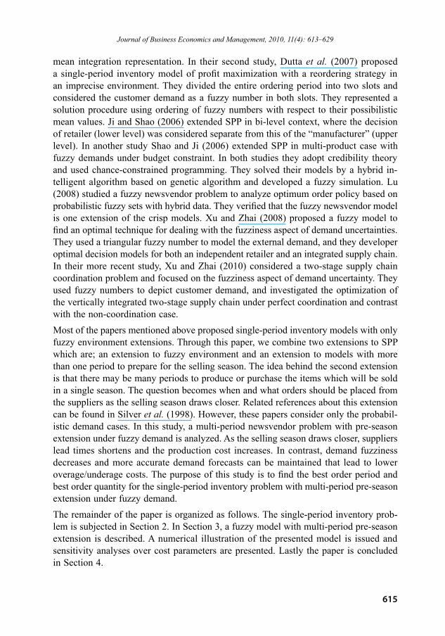
Let us show a fuzzy number ( , , , )l m n uX x x x x= where l m n ux x x x< < < in this form. The fuzzy number X is a so-called triangular fuzzy number ( , , )l m n uX x x x x= = ,

l m n ux x x x< = < if its membership function

[ ]( ) : 0,1X x Rµ → is equal to (Fig. 1):

0

( ) .

0 x>x

l

ll m

m lX u

m uu m

u

x x

x xx x x

x xx x xx x x

x x

<

− < < − µ = − < < −

(11)

The fuzzy function X is a function of parameters , and l m ux x x , known as the lower value, middle value and upper value respectively. The figure (Fig. 1) shows the member-ship function for a fuzzy number “approximately xm”.In this study, a multi-period newsvendor problem with pre-season extension under fuzzy demand is analyzed. As the selling season draws closer, suppliers lead times shortens and the production cost increases. In contrast, demand fuzziness decreases and more accurate demand forecasts can be maintained that lead to lower overage/underage costs.The purpose of the model is to find the best order period (M*) and best order quantity (Q*)for the multi-period newsvendor problem with pre-season extension under discrete fuzzy demand X with membership function

( )iX xµ , precise production cost cp, fuzzy unit holding cost hc with

hcµ and fuzzy unit shortage sc cost with

scµ .

3.1. Fuzzy demand and fuzzy inventory costs with precise purchasing costLet the membership function

( )iX xµ of fuzzy demand X given by domain

0 1 2{ , , ,..., }nX x x x x= have the triangular membership function (Fig. 1). Unit produc-tion cost, (cp) is precise while unit holding cost ( )hc and unit shortage cost ( )sc , are represented by triangular fuzzy numbers. The uncertain demand and uncertain cost

Fig. 1. Triangular membership function

xl xm xu x

1.0

0

�� ( )X

x

H. Behret, C. Kahraman. A multi-period newsvendor problem with pre-season extension under fuzzy demand

619

parameters cause uncertain overage and underage costs. For a given Q and

ix X∈ , the fuzzy overage ( )OC and underage costs ( )UC , are as follows;

( ){ } ( ){ }

max ,0

max ,0 .h

s

OC c Q X

UC c X Q

= −

= − (12)

The unit penalty cost ( )PC is the sum of unit overage cost and unit underage cost with the membership function

PCµ . .PC OC UC= + (13)

The unit penalty cost ( )PC ) is a level-2 fuzzy set which means that it includes two fuzzy values and there are corresponding membership degrees of these fuzzy values.A level-2 fuzzy set can be reduced to an ordinary fuzzy set by s-fuzzification process (Zadeh 1971). The membership function of an ordinary fuzzy set is maintained via s-fuzzification (“s” stands for support) as follows:

0,1,2,...,( ) ( ) sup [ ( ) ( )], ,ii n cs fuzz PC PCx i x x X=−µ = µ ×µ ∈

(14)

where ci(x) is the ith possible fuzzy cost of PC and

( )PC iµ is the possibility of that cost.According to the properties of possibility measure (Zadeh 1978),

( )PC iµ is ob-tained as follows:

( ) max ( ), 0,1,2,..., .i ix X XPC i x i n∈µ = µ =

(15)

The fuzzy total cost is minimized by the best order quantity (Q*):

*( , ) min ( ( )) .Q pTC Q X c Q defuzz s fuzz PC = + −

(16)

Here, the operator “defuzz” denotes the defuzzification process. Defuzzification is the conversion of a fuzzy quantity to a precise quantity; in contrast fuzzification is the conversion of a precise quantity to a fuzzy quantity. Usually, a fuzzy system will have a number of rules that transform a number of variables into a “fuzzy” result. Defuzzifi-cation would transform this result into a single number (Ross 1995). There are several methods for defuzzification. In this study centroid defuzzification method is applied. Centroid defuzzification method (also called center of area, center of gravity) is the most common of all the defuzzification methods. It is given by the algebraic expression as follows.For continuous functions:

( )*

( )

.C z

C z

zdzz

dz

µ=

µ

∫∫

(17)

For discrete functions:

( )*

( )

,C z

C z

zz

µ=

µ

∑∑

(18)

where ( ) 1z

z i iC C==

and iC is one of the membership functions those figure the fuzzy

output. This method is represented in Fig. 2.

Journal of Business Economics and Management, 2010, 11(4): 613–629

620

Best order quantity (Q*) which minimiz-es the fuzzy total cost is found by brute-force search algorithm which is a very general problem-solving technique that consists of systematically enumerating all possible candidates for the solution and checking whether each candidate satisfies the problem’s statement.

The procedure explained above is exam-ined for every pre-season ordering period. Through these periods as the selling sea-

son draws closer the production cost increases and demand fuzziness decreases and more accurate demand forecasts can be maintained that lead to lower overage/underage costs.

In the multi-period model, jpc denotes unit production cost for period j. Demand fuzzi-

ness decreases as the ordering period closes to the selling season. This decrease of fuzziness is maintained by fuzzy concentration of the membership function of demand according to the periods. The membership function

( )iX xµ of fuzzy demand X is given by domain 0 1 2{ , , ,..., }nX x x x x= concentrates as the selling season draws closer.

Concentrations tend to concentrate the element of a fuzzy set by reducing the degree of membership of all elements that have lower membership degrees in the set. The less an element is in a set, the more it is reduced in membership through concentration (Ross 1995).

The membership function of fuzzy demand for period j is denoted by

( )j iX xµ . Fuzzy

total cost for pre-season ordering periods is as follows:

*( , ) min [ ( ( ))].

j jj jj Q p jTC Q X c Q defuzz s fuzz PC= + − (19)

Here jPC represents the penalty cost for period j where j=1,2,...,m. The best order period *( )M is the period which has the minimum fuzzy total cost.

3.2. Numerical illustrationSuppose that a retailer wants to introduce an innovative product to the market at the beginning of July and have six possible periods (January, February, March, April, May, June) to give the manufacturing order to the manufacturer. As the selling season draws closer, suppliers lead times shorten and the production cost increases. On the other hand demand fuzziness decreases and more accurate demand forecasts can be maintained that lead to lower overage/underage costs.

Let unit holding cost ( )hc and unit shortage cost ( )sc be imprecise and represented with triangular fuzzy numbers as, [ ]$ 1,2,3hc = and [ ]$ 4,5,6sc = , respectively. Unit purchasing cost is precise and increases 5% according to the previous months’ cost Table 1.

Fig. 2. Centroid defuzzification method

�

1

z* z

H. Behret, C. Kahraman. A multi-period newsvendor problem with pre-season extension under fuzzy demand

621

Table 1. Unit purchasing cost per month ($)

Jan Feb March April May June

3.50 3.68 3.86 4.05 4.25 4.47

Let the membership function

( )iX xµ of fuzzy demand X for January be {1000,1500,2000,2500,3000,3500,4000,4500,5000,5500,6000}X = with the triangu-lar membership function as follows:

0 1000

1000 1000 3500

2500( ) . 6000 3500 6000

2500

0 x >6000

i

ii

iX ii

i

x

xx

x xx

<

− < < µ = − < <

(20)

For example let x1 = 1000. The membership value of x1 will be 1( ) 0X xµ = or if x7 =

1000 then the membership value of x7 will be 7( ) 0.80X xµ = and so on. The member-

ship functions for other months are maintained through the membership function of the demand for January using fuzzy concentration (Table 2 and Fig. 3).

Table 2. Membership values of demand per month

Jan Feb March April May June

Demand

( )iX xµ

1.25( )iX xµ

1.5( )iX xµ

2( )iX xµ

3( )iX xµ

4( )iX xµ

1000 0.000 0.000 0.000 0.000 0.000 0.000

1500 0.200 0.134 0.089 0.040 0.008 0.002

2000 0.400 0.318 0.253 0.160 0.064 0.026

2500 0.600 0.528 0.465 0.360 0.216 0.130

3000 0.800 0.757 0.716 0.640 0.512 0.410

3500 1.000 1.000 1.000 1.000 1.000 1.000

4000 0.800 0.757 0.716 0.640 0.512 0.410

4500 0.600 0.528 0.465 0.360 0.216 0.130

5000 0.400 0.318 0.253 0.160 0.064 0.026

5500 0.200 0.134 0.089 0.040 0.008 0.002

6000 0.000 0.000 0.000 0.000 0.000 0.000

Journal of Business Economics and Management, 2010, 11(4): 613–629

622

For example, let us order a quantity of 2000 units at the beginning of January. The unit pen-alty cost ( )PC is a level-2 fuzzy set including imprecise demand and costs. For x1 = 1000, the fuzzy penalty cost will be (1,2,3) 1000 (1000,2000,3000)PC = × = with possibility of 0. For x5 = 3000, the fuzzy penalty cost will be (4,5,6) 1000 (4000,5000,6000)PC = × = with the possibility 0.80 and so on. For the ordering period January fuzzy unit penalty cost values for Q = 2000 is given in Table 3.The graphical representations of level-2 fuzzy sets of ( )PC for January when Q = 2000 and the corresponding s-fuzzified set ( )s fuzz PC− are shown in Figs. 4a and 4b, respectively.

Table 3. Unit penalty cost values for January, Q = 2000

X

( )xiXµ ( )OC ( )UC ( )PC

x1 1000 0 (1000,2000,3000) (0,0,0) (1000,2000,3000)

x2 1500 0.20 (500,1000,1500) (0,0,0) (500,1000,1500)

x3 2000 0.40 (0,0,0) (0,0,0) (0,0,0)

x4 2500 0.60 (0,0,0) (2000,2500,3000) (2000,2500,3000)

x5 3000 0.80 (0,0,0) (4000,5000,6000) (4000,5000,6000)

x6 3500 1 (0,0,0) (6000,7500,9000) (6000,7500,9000)

x7 4000 0.80 (0,0,0) (8000,10000,12000) (8000,10000,12000)

x8 4500 0.60 (0,0,0) (10000,12500,15000) (10000,12500,15000)

x9 5000 0.40 (0,0,0) (12000,15000,18000) (12000,15000,18000)

x10 5500 0.20 (0,0,0) (14000,17500,21000) (14000,17500,21000)

x11 6000 0 (0,0,0) (16000,20000,24000) (16000,20000,24000)

Fig. 3. Fuzzy concentration of X

�� ( )iXx

1000 1500 2000 2500 3000 3500 4000 4500 5000 5500 6000

January

February

March

April

May

June

1.000

0.900

0.800

0.700

0.600

0.500

0.400

0.300

0.200

0.100

0.000

Fuzzy Concentration of �X

xi

H. Behret, C. Kahraman. A multi-period newsvendor problem with pre-season extension under fuzzy demand

623

According to the s-fuzzified value of the penalty cost, total cost for the given values when Q = 2000 is calculated as below:

(2000, ) [3.50 2000 ( ( ))].TC X defuzz s fuzz PC= × + − (21)

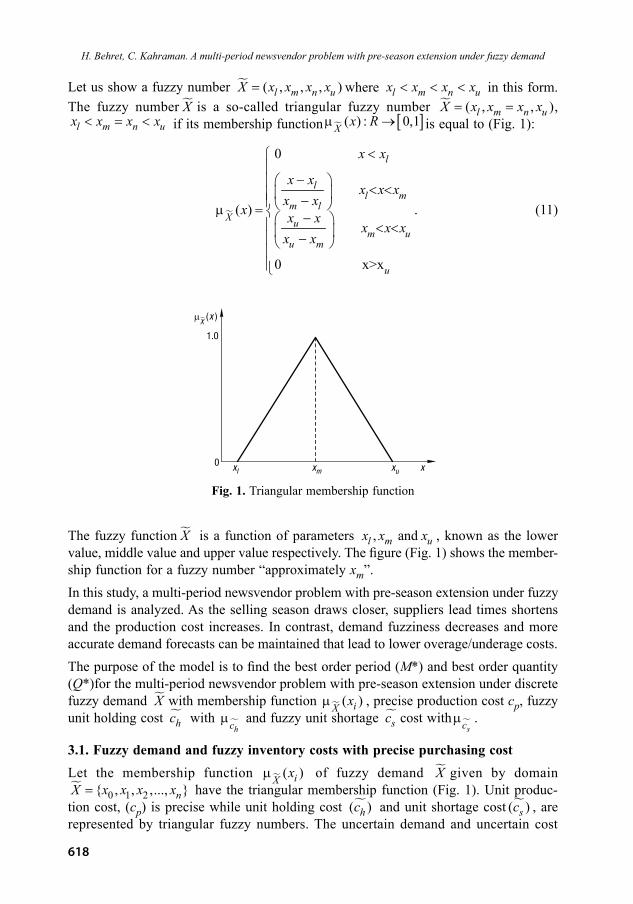
Here, the operator “defuzz” denotes the centroid method for defuzzification. Centroid defuzzification values have been obtained by using MATLAB R2008a Fuzzy Logic Toolbox as in Fig. 5.

(2000, ) [3.5 2000 10,022] $17,022TC X = × + = . (22)

Fuzzy total cost values for all other order quantities of the ordering period January are given in Table 4. For the ordering period January, best order quantity which gives the min fuzzy total cost is found 3000 units with the fuzzy total cost value $16,820.The procedure continues with calculation of other periods best order quantities. Using Equation 19, the fuzzy total costs for pre-season ordering periods are calculated and given as in Table 5 and Fig. 6.As stated by Table 5, best order period (M*) is found January with fuzzy total cost $16,820 with 3000 units. Here the decrease of demand fuzziness causes a decline on the fuzzy total cost values among ordering periods. However, the change of production cost also affects the cost function. The proposed model offers best order period and corresponding order quantity for the given fuzzy variables.

Fig. 4a. Level-2 fuzzy set ( )PC

Fig. 4b. ( )s fuzz PC−

�� ( )PC

i

0 1 2 3 4 5 6 7 8 9 10 11 12 13 14 15 16 17 18 19 20 21 22 23 24� �( $1000)PC

i = 1 2 4 5 6 7 8 9 10 111

0 1 2 3 4 5 6 7 8 9 10 11 12 13 14 15 16 17 18 19 20 21 22 23 24� �( $1000)PC

0,2

0,4

0,6

0,8

1

Journal of Business Economics and Management, 2010, 11(4): 613–629

624

Fig. 5. Centroid defuzzification of ( )s fuzz PC−

1

0.9

0.8

0.7

0.6

0.5

0.4

0.3

0.2

0.1

0

0 0.5 1 1.5 2 2.5 3

x104Centroid

Table 4. Fuzzy total costs for January, ($)

Order quantity Fuzzy total cost1000 17,356

1500 17,159

2000 17,0222500 16,9303000 16,820*3500 16,8284000 17,2584500 19,0795000 21,5145500 24,0456000 26,681

Table 5. Fuzzy total cost for pre-season ordering periods, [ ] [ ]$ , $1,2,3 4,5,6h sc c= =

Q ( )TC Jan ( )TC Feb ( )TC March ( )TC April ( )TC May ( )TC June

cp 3,50 3,68 3,86 4,05 4,25 4,47

1000 17,356 17,335 17,360 17,327 17,262 17,332

1500 17,159 17,161 17,219 17,184* 17,098 17,202

2000 17,022 17,089 17,210* 17,202 17,087* 17,202*

2500 16,930 17,082 17,282 17,333 17,223 17,350

3000 16,820* 17,075* 17,375 17,515 17,448 17,617

3500 16,828 17,168 17,553 17,787 17,815 18,087

4000 17,258 17,718 18,237 18,659 19,003 19,589

4500 19,079 19,709 20,401 21,063 21,708 22,508

5000 21,514 22,252 23,059 23,861 24,678 25,636

5500 24,045 24,902 25,831 26,775 27,756 28,843

6000 26,681 27,658 28,703 29,778 30,880 32,058

H. Behret, C. Kahraman. A multi-period newsvendor problem with pre-season extension under fuzzy demand

625

3.3. Sensitivity analysis

In this section, various experiments have been performed to analyze the effect of mem-bership function shapes to the fuzzy models. Through these experiments fuzzy unit holding cost and fuzzy unit shortage cost values have been changed (Table 6).

Table 6. Performed experiments and values of the cost parameters

Experiments ($)hc ($)sc

1 (1,2,3) (4,5,6)2 (1,2,3) (4,5,8)3 (1,2,3) (4,5,10)4 (1,2,3) (4,5,12)5 (1,2,5) (4,5,6)6 (1,2,5) (4,5,8)7 (1,2,5) (4,5,10)8 (1,2,5) (4,5,12)9 (1,2,7) (4,5,6)10 (1,2,7) (4,5,8)11 (1,2,7) (4,5,10)12 (1,2,7) (4,5,12)13 (1,2,9) (4,5,6)14 (1,2,9) (4,5,8)15 (1,2,9) (4,5,10)16 (1,2,9) (4,5,12)

Q

30 000

25 000

20 000

15 000

�TC

1000 1500 2000 2500 3000 3500 4000 4500 5000 5500 6000

January

February

March

April

May

June

Fig. 6. Fuzzy total cost for pre-season ordering periods

Journal of Business Economics and Management, 2010, 11(4): 613–629

626

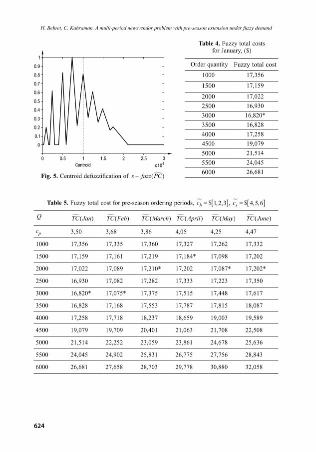
In these experiments, production cost values and demand membership functions are considered the same as the previous illustration while the membership of holding cost and the membership of shortage cost have been changed. According to the provided membership values, the fuzzy model generates the results represented in Table 7.

Table 7. *M , *Q and TC for different hc and sc

Experiments *M *Q ($)TC

1 Jan 3000 16,820

2 Jan 2500 17,716

3 May 2500 18,484

4 June 3000 19,152

5 Jan 3000 16,626

6 Jan 3000 17,619

7 May 2500 18,457

8 May 3000 19,093

9 Jan 3000 16,509

10 Jan 3000 17,545

11 May 3000 18,431

12 May 3000 19,062

13 Jan 3000 16,449

14 Jan 3000 17,498

15 May 3000 18,417

16 May 3000 19,048

The results provided in Table 7 represents that, the increase of the fuzziness of cost parameters causes an increase of fuzzy total cost values. For example, in experiment 2, we increased the fuzziness of shortage cost by changing the membership function shape to [ ]$ 4,5,8sc = . This change increased the fuzzy total cost value from $16,820 to $17,716. Shortage cost values as they have higher fuzziness affect the order period in that way. In experiments 3 and 4 membership values of shortage costs are wider than the values in experiments 1 and 2. For the experiments 1 and 2 best order period is found as January which has the maximum demand fuzziness and minimum production cost. However, for experiments 3 and 4 best order period changes to May and June, respectively, which have minimum demand fuzziness and maximum production costs.Best order quantities for the experiments do not change much according to different sce-narios. The reason of this situation is the symmetrical shape of demands’ membership function. Only in three experiments best order quantity decreases from 3000 to 2500. If nonsymmetrical membership functions are used for demand data, more changes on offered order quantities can be observed.

H. Behret, C. Kahraman. A multi-period newsvendor problem with pre-season extension under fuzzy demand

627

4. Conclusion

The classical single-period inventory problem has been considered extensively in the relevant literature. Through these studies, most of the extensions have been made in the probabilistic and possibilistic framework. Most of the papers under possibilistic frame-work proposed single-period inventory models with only fuzzy environment extensions. Through this paper, we combine two extensions to single-period inventory problem which are; an extension to fuzzy environment and an extension to models with more than one period to prepare for the selling season. The model is developed for innovative products. The demand, holding and shortage cost parameters are represented by fuzzy numbers. The model has been experimented with an illustrative example and supported by sensitivity analyses.Contrary to the crisp model, fuzzy model proposes highly flexible solutions for all pos-sible states. When the solutions of the model are analyzed, it is seen that the decrease of demand fuzziness causes a decline on the fuzzy total cost values among ordering peri-ods. The fuzzy model offers the best order period and corresponding order quantity for the given fuzzy variables. Furthermore, the increase of the fuzziness of cost parameters causes an increase in fuzzy total cost values. Shortage cost values as they have higher fuzziness affect the order period in that way. Best order quantities for the experiments do not change much according to different scenarios. The reason of this situation is the symmetrical shape of demands’ membership function.For further research, we suggest the examination of the influence of nonsymmetrical and different type of membership functions for demand data on order quantities. Further-more, the use of an imprecise continuous demand function instead of the discrete case of this paper can be examined. This will require optimization techniques for solution procedure. Lastly, dependent demand structure among ordering periods is suggested to be applied.

ReferencesDubois, D.; Prade, H. 1980. Fuzzy Sets and Systems: Theory and Applications. New York: Aca-demic Press.Dutta, P.; Chakraborty, D.; Roy, A. R. 2005. A single-period inventory model with fuzzy random variable demand, Mathematical and Computer Modelling 41(8–9): 915–922. doi:10.1016/j.mcm.2004.08.007Dutta, P.; Chakraborty, D.; Roy, A. R. 2007. An inventory model for single-period products with reordering opportunities under fuzzy demand, Computers & Mathematics with Applications 53(10): 1502–1517. doi:10.1016/j.camwa.2006.04.029Ishii, H.; Konno, T. 1998. A stochastic inventory problem with fuzzy shortage cost, European Journal of Operational Research 106(1): 90–94. doi:10.1016/S0377-2217(97)00173-2Ji, X. Y.; Shao, Z. 2006. Model and algorithm for bilevel newsboy problem with fuzzy demands and discounts, Applied Mathematics and Computation 172(1): 163–174. doi:10.1016/j.amc.2005.01.139Kao, C.; Hsu, W.-K. 2002. A single-period inventory model with fuzzy demand, Computers & Mathematics with Applications 43(6–7): 841–848. doi:10.1016/S0898-1221(01)00325-X

Journal of Business Economics and Management, 2010, 11(4): 613–629

628

Khouja, M. 1999. The single-period (news-vendor) problem: literature review and suggestions for future research, Omega – International Journal of Management Science 27(5): 537–553. doi:10.1016/S0305-0483(99)00017-1Kopytov, E.; Greenglaz, L.; Tissen, F. 2006. Stochastic inventory control model with two stages in ordering process, Journal of Business Economics and Management 7(1): 21–24.Lee, H. L. 2002. Aligning supply chain strategies with product uncertainties, California Manage-ment Review 44(3): 105–119.Li, L. S.; Kabadi, S. N.; Nair, K. P. K. 2002. Fuzzy models for single-period inventory problem, Fuzzy Sets and Systems 132(3): 273–289. doi:10.1016/S0165-0114(02)00104-5Lu, H.-F. 2008. A fuzzy newsvendor problem with hybrid data of demand, Journal of the Chinese Institute of Industrial Engineers 25(6): 472–480. doi:10.1080/10170660809509109Nahmias, S. 1996. Production and Operations Management. Third edition. Boston MA: Irwin.Petrovic, D.; Petrovic, R.; Vujosevic, M. 1996. Fuzzy models for the newsboy problem, Interna-tional Journal of Production Economics 45(1–3): 435–441. doi:10.1016/0925-5273(96)00014-XRoss, T. J. 1995. Fuzzy Logic with Engineering Applications. 2nd edition. New York:McGraw-Hill.Shao, Z.; Ji, X. 2006. Fuzzy multi-product constraint newsboy problem, Applied Mathematics and Computation 180(1): 7–15. doi:10.1016/j.amc.2005.11.123Silver, E. A.; Pyke, D. F.; Peterson, R. P. 1998. Inventory Management and Production Planning and Scheduling. Third edition. New York: John Wiley.Xu, R.; Zhai, X. 2008. Optimal models for single-period supply chain problems with fuzzy de-mand, Information Sciences 178(17): 3374–3381. doi:10.1016/j.ins.2008.05.012Xu, R.; Zhai, X. 2010. Analysis of supply chain coordination under fuzzy demand in a two-stage supply chain, Applied Mathematical Modeling 34(1): 129–139. doi:10.1016/j.apm.2009.03.032Zadeh, L. A. 1965. Fuzzy sets, Information and Control 8(3): 338–353. doi:10.1016/S0019-9958(65)90241-XZadeh, L. A. 1971. Quantitative fuzzy semantics, Information Science 3(2): 159–176. doi:10.1016/S0020-0255(71)80004-XZadeh, L. A. 1978. Fuzzy sets as a basis for a theory of possibility, Fuzzy Sets and Systems 100(1): 9–34.

H. Behret, C. Kahraman. A multi-period newsvendor problem with pre-season extension under fuzzy demand

629

KELIŲ LAIKOTARPIŲ PARDAVIMŲ MODELIS, PAPILDYTAS PARUOŠIAMUOJU LAIKOTARPIU, ESANT NERAIŠKIAJAI PAKLAUSAI

H. Behret, C. Kahraman

Santrauka

Straipsnyje pasiūlytas neraiškusis kelių laikotarpių pardavimo modelis, papildytas paruošiamuoju lai-kotarpiu inovatyviems produktams. Produkto paklausa apibūdinama neraiškiaisiais skaičiais, aprašytais trikampe priklausomumo funkcija. Turto ir sąnaudų parametrai laikomi netiksliais ir taip pat apibūdi-nami trikampe priklausomumo funkcija aprašytais neraiškiaisiais skaičiais. Kai pardavimo laikotarpis priartėja, tiekimo laikas trumpėja, o gaminio kaina išauga. Priešingai, dėl praeinančio pardavimo laiko-tarpio paklausos neapibrėžtumas sumažėja ir galima tiksliau prognozuoti paklausą, o tai padeda suma-žinti išlaidas dėl gaminių pertekliaus ar trūkumo. Šio modelio tikslas – rasti geriausią užsakymo laiką ir geriausią užsakymo kiekį, kurie padėtų sumažinti visų numatomų sąnaudų neapibrėžtumą. Pateikiamas modelio taikymo pavyzdys ir modelio jautrumo analizė.

Reikšminiai žodžiai: atsargų problema, neraiškusis modeliavimas, pardavimas, inovatyvus produktas, neraiškioji paklausa, neraiškioji atsargų savikaina, paruošiamasis laikotarpis.

Hülya BEHRET. M. Sc., a research assistant at Istanbul Technical University, Industrial Engineering Department and working on her PhD dissertation on “Fuzzy Single-Period Inventory Models in Pro-duction Systems” under the supervision of Prof. Cengiz Kahraman. Her research areas are Production and Inventory Systems, Fuzzy Modeling, and Simulation.

Cengiz KAHRAMAN. A professor of industrial engineering at Istanbul Technical University, Indus-trial Engineering Department. He has published about 100 international journal papers and 50 interna-tional book chapters on fuzzy applications of industrial engineering. His research areas are engineering economics, quality control and management, statistical decision making, and production engineering.

Journal of Business Economics and Management, 2010, 11(4): 613–629