Autonomous Robots manuscript No.(will be inserted by the editor)

A provably complete exploration strategy by constructingVoronoi diagrams

Jonghoek Kim · Fumin Zhang · Magnus Egerstedt

Received: date / Accepted: date

Abstract We present novel exploration algorithms thatenable the construction of Voronoi diagrams over un-

known areas using a vehicle equipped with range sen-sors. The underlying control law uses range measure-ments to make the vehicle track Voronoi edges between

obstacles. The exploration algorithms make decisionsat vertices in the Voronoi diagram to expand the ex-plored area until a complete Voronoi diagram is con-

structed in finite time. Our exploration algorithms areprovably complete, and the convergence of the controllaw is guaranteed. Simulations and experimental results

are provided to demonstrate the effectiveness of boththe control law and the exploration algorithms.

Keywords Voronoi Diagrams · Map-making Algo-rithms · Robot Control

1 Introduction

This paper addresses the problem of exploring an un-known workspace using a vehicle equipped with rangesensors. Such sensors have the ability to determine a

point on an obstacle boundary that is closest to the ve-hicle. We call such a point the closest point. If obstacleboundaries appear on both sides of the vehicle, then

a closest point can be determined on each boundary.A path that is at an equal distance from these closestpoints is a Voronoi edge. All such Voronoi edges form

the Voronoi diagram that reveals the topological struc-ture of the workspace. If the vehicle visits all Voronoi

Jonghoek Kim · Fumin Zhang · Magnus Egerstedt

School of Electrical and Computer Engineering,Georgia Institute of Technology, USAE-mail: jkim37@gatech.edu

fumin@gatech.edumagnus@ece.gatech.edu

edges in the workspace, then we consider the workspaceas being completely explored.

Voronoi diagrams have been widely used in vari-

ous areas such as biology [6,24], computational geome-try [15,19,20,28], VLSI design [32], and sensor networks[3,12,23]. In robotics, Voronoi diagrams have been uti-

lized to obtain paths that satisfy minimum clearancerequirements [1, 4, 16, 29, 34]. Voronoi diagrams can begeneralized from two to higher dimensions, and also fita wide class of robots with higher dimensional config-

uration spaces [7,8]. Several extensions of Voronoi dia-grams have been developed by other researchers, includ-ing the generalized Voronoi graphs (GVG), the hiearchi-

cal GVG (HGVG) and the reduced GVG (RGVG)1 in[7,10,11,26]. The exploration of an unknown workspaceby incrementally constructing the Voronoi diagram was

previously achieved in [8,29,33]. But, the convergence ofthe algorithms was not proved in the above references.

In order for the vehicle to follow a Voronoi edge,we develop a Voronoi edge tracking control law that is

provably convergent. This law is based on the shapedynamics derived in [36] and [38], where a gyroscopicfeedback control law was developed to control the inter-

action between the vehicle and the closest point so thatthe vehicle follows the obstacle boundary either to theleft or to the right. This controller design method wasgeneralized to cooperative motion patterns on closed

curves for multiple vehicles in [35, 37], and extendedto the design of pursuit-evasion laws in three dimen-sions [30]. The closest point was also used for path fol-

lowing in earlier works such as [31]. Our curve trackingcontrol law extends previous works by using informa-tion from the closest points on both sides of the vehicle.

1 Our notion of Voronoi diagrams is similar to the RGVG in

that no Voronoi edge is connected to the obstacle boundaries.

2

This results in a tracking behavior of the Voronoi edge

between two obstacles.

To make a robot track a Voronoi edge, the authorsof [8] used a numerical continuation method that re-

lies on two iterative stages : a prediction step and acorrection procedure. Since the prediction step makesthe robot move off the GVG edge, this continuation

method may produce zigzag movements of the robot [9].Furthermore, after the correction procedure, the robotmust rotate again to re-orient itself on a Voronoi edge.

These rotations may take time and cause additionalwheel slippage [9]. Later, a control law was presentedin [9], which provided a smoother path than the nu-

merical continuation method [8]. However, smoothnessof the robot’s trajectory was not ensured. Note thatthe curvature of obstacle boundaries was not consid-

ered in [8, 9]. In contrast, our tracking control law uti-lizes estimated curvature that is well defined along thetrajectory of the vehicle. Hence, we can guarantee that

the trajectory of the vehicle is smooth.

Utilizing the Voronoi edge tracking behavior, we

develop provably complete exploration algorithms, de-noted as the boundary expansion (BE) algorithms, whichenable the construction of a topological map based on

Voronoi diagrams. Although many results exist in liter-ature regarding the construction of Voronoi diagrams,to our knowledge, the BE algorithms are unique, with

provable completeness over a compact workspace.

The BE algorithms are composed of two algorithms,denoted by Algorithm 1 and Algorithm 2 in this paper.

Applying Algorithm 1, the trajectory of a vehicle con-structs a simple closed curve that encloses an obstacleto its right. Then, using Algorithm 2, the vehicle itera-

tively expands the explored area in such a way that oneobstacle is added to the area at a time. In this way, thevehicle constructs a Voronoi diagram by “expanding”

the explored area in discrete and finite steps.

In the BE algorithms, only the graph structure rep-

resenting the boundary of the explored area is main-tained and updated based on two simple rules. Thereis no need to explicitly search for the shortest path

in the graph as in many other exploration algorithms[10, 29, 33]. Hence, the BE algorithms may have lowercomputational load.

We implement the algorithms and the control lawon a miniature robot localizing itself based on an odom-etry system. The robot uses only Infrared (IR) sensors

for range measurements. Both simulations and experi-mental results demonstrate the effectiveness of the al-gorithms.

The paper is organized as follows. Section 2 presentsthe workspace to be explored. Section 3 introduces the

provably convergent control law to track Voronoi edges.

Section 4 discusses the BE algorithms. Section 5 pro-

vides proofs for the convergence of the BE algorithms.Section 6 analyzes the efficiency of the BE algorithms.Section 7 demonstrates simulation and experimental re-

sults, and Section 8 provides conclusions.

2 The Workspace and Its Voronoi Diagram

Consider a connected and compact workspace W ⊂ R2

whose boundary, ∂W , is a regular curve. LetO1,O2,...OM−1

be M − 1 disjoint and compact obstacles such that

Oi ⊂ W . OM is a “virtual” obstacle that bounds theworkspace, i.e., ∂W ⊂ ∂OM . We denote the set of ob-stacles SO by SO = O1, O2, ..., OM.

Obeying the conventions established in the litera-

ture on Voronoi diagrams [2,7,20,21,26], we define theVoronoi cell for an obstacle Oi as the set of points thatis closer to Oi than to any other obstacle in SO for

i = 1, 2, ...,M i.e.

V (Oi) = q ∈ W | minz∈Oi

∥z − q∥ < minz′∈O′

i

∥z′ − q∥,

∀O′i ∈ SO \Oi, (1)

where ∥ · ∥ is the Euclidean norm in R2. ∂V (Oi) is the

boundary of the Voronoi cell for Oi, i.e., V (Oi). Also,V (Oi) = V (Oi)

∪∂V (Oi). The Voronoi diagram of the

workspace is defined as the union of all cell boundaries

[20] i.e.

D(W ) =∪

Oi∈SO

∂V (Oi). (2)

The shared boundary between two Voronoi cells is a

Voronoi edge. More specifically, a Voronoi edge betweentwo Voronoi cells V (Oi) and V (Oj) is defined by

Eij = ∂V (Oi)∩

∂V (Oj). (3)

3 Tracking a Voronoi edge

In this section, we develop a feedback control law to

make a vehicle, with its dynamics approximated by aunit speed particle, move along a Voronoi edge. We as-sume that the range sensors of the vehicle can detect

two obstacle boundaries, each on one side of the vehi-cle. Then, on each obstacle boundary, the vehicle candetermine a closest point to itself. The feedback control

law uses measurements at the two closest points.

We first introduce the shape dynamics that governthe relationship between the vehicle and the closestpoints. We then derive the tracking control law, and

prove its convergence.

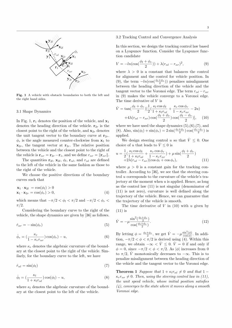
3

x2r

y2r r2r

x2l

y2l

r2l

x2r

x2l

x1y1

r1−φl

φr

rαr

rαl

Fig. 1 A vehicle with obstacle boundaries to both the left andthe right hand sides.

3.1 Shape Dynamics

In Fig. 1, r1 denotes the position of the vehicle, and x1

denotes the heading direction of the vehicle. r2r is theclosest point to the right of the vehicle, and x2r denotesthe unit tangent vector to the boundary curve at r2r.

ϕr is the angle measured counter-clockwise from x1 tox2r, the tangent vector at r2r. The relative positionbetween the vehicle and the closest point to the right of

the vehicle is rαr = r2r−r1, and we define rαr = ∥rαr∥.The quantities r2l, x2l, ϕl, rαl, and rαl are defined

to the left of the vehicle in the same fashion as those tothe right of the vehicle.

We choose the positive directions of the boundarycurves such that

x1 · x2l = cos(ϕl) > 0x1 · x2r = cos(ϕr) > 0, (4)

which means that −π/2 < ϕl < π/2 and −π/2 < ϕr <π/2.

Considering the boundary curve to the right of thevehicle, the shape dynamics are given by [36] as follows.

rαr = − sin(ϕr) (5)

ϕr = (κr

1− κrrαr) cos(ϕr)− u, (6)

where κr denotes the algebraic curvature of the bound-ary at the closest point to the right of the vehicle. Sim-

ilarly, for the boundary curve to the left, we have

rαl = sin(ϕl) (7)

ϕl = (κl

1 + κlrαl) cos(ϕl)− u, (8)

where κl denotes the algebraic curvature of the bound-

ary at the closest point to the left of the vehicle.

3.2 Tracking Control and Convergence Analysis

In this section, we design the tracking control law basedon a Lyapunov function. Consider the Lyapunov func-

tion candidate

V = −ln(cos(ϕl + ϕr

2)) + λ(rαl − rαr)

2, (9)

where λ > 0 is a constant that balances the controlfor alignment and the control for vehicle position. In

(9), the term −ln(cos(ϕl+ϕr

2 )) penalizes misalignmentbetween the heading direction of the vehicle and thetangent vector to the Voronoi edge. The term rαl − rαrin (9) makes the vehicle converge to a Voronoi edge.The time derivative of V is

V = tan(ϕl + ϕr

2)[1

2(κl cosϕl

1 + κlrαl+

κr cosϕr

1− κrrαr− 2u)

+4λ(rαl − rαr) cos(ϕl + ϕr

2) cos(

ϕl − ϕr

2)], (10)

where we have used the shape dynamics (5),(6),(7), and

(8). Also, sin(ϕl) + sin(ϕr) = 2 sin(ϕl+ϕr

2 ) cos(ϕl−ϕr

2 ) isapplied.

We design steering control u so that V ≤ 0. One

choice of u that leads to V ≤ 0 is

u =1

2(κl cosϕl

1 + κlrαl+

κr cosϕr

1− κrrαr) + µ sin(

ϕl + ϕr

2)

+2λ(rαl − rαr)(cosϕl + cosϕr), (11)

where µ > 0 is a constant gain for the tracking con-troller. According to [36], we see that the steering con-trol u corresponds to the curvature of the vehicle’s tra-

jectory at the moment when u is applied. Hence, as longas the control law (11) is not singular (denominator of(11) is not zero), curvature is well defined along the

trajectory of the vehicle. Hence, we can guarantee thatthe trajectory of the vehicle is smooth.

The time derivative of V in (10) with u given by

(11) is

V = −µsin2(ϕl+ϕr

2 )

cos(ϕl+ϕr

2 ). (12)

By letting ϕ = ϕl+ϕr

2 , we get V = −µ sin2(ϕ)cos(ϕ) . In addi-

tion, −π/2 < ϕ < π/2 is derived using (4). Within thisrange, we obtain −∞ < V ≤ 0. V = 0 if and only ifϕ = 0, since −π/2 < ϕ < π/2. As |ϕ| increases from 0

to π/2, V monotonically decreases to −∞. This is topenalize misalignment between the heading direction ofthe vehicle and the tangent vector to the Voronoi edge.

Theorem 1 Suppose that 1 + κlrαl = 0 and that 1 −κrrαr = 0. Then, using the steering control law in (11),the unit speed vehicle, whose initial position satisfies

(4), converges to the state where it moves along a smoothVoronoi edge.

4

Proof For each trajectory that initially satisfies (4),

there exists a compact sublevel set Ω of V such thatthe trajectory remains in Ω for all future time. Then, byLaSalle’s Invariance Principle [17], the trajectory con-

verges to the largest invariant set I within the set Ethat contains all points in Ω where V = 0. The setE in this case is the set of all points in Ω such that

ϕl +ϕr = 0. Thus, at any point in E, the dynamics areexpressed as

E = (rαl, rαr, ϕl, ϕr)|ϕl + ϕr = 0. (13)

Since the trajectory converges to the largest invari-ant set I within the set E, we obtain ϕl + ϕr = 0 in I.Therefore, using (6) and (8), we derive

(κr

1− κrrαr) cos(ϕr)+(

κl

1 + κlrαl) cos(ϕl)−2u = 0. (14)

Applying (11), we get

2λ(rαl − rαr)(cos(ϕl) + cos(ϕr)) + µ sin(ϕl + ϕr

2) = 0.

(15)

In order to satisfy (15), rαl − rαr = 0 is required, sinceϕl + ϕr = 0 inside the set E. Therefore, the largest

invariant set I is expressed as

I = (rαl, rαr, ϕl, ϕr)|rαl = rαr, ϕl + ϕr = 0. (16)

Thus, we can conclude that (rαl, rαr, ϕl, ϕr) convergesto the equilibrium where rαl = rαr and ϕl = −ϕr. Ifthe vehicle is equidistant from two closest points on the

obstacle boundaries and the heading direction of thevehicle is aligned to the tangent vector to the Voronoiedge, then the vehicle moves along the Voronoi edge.

This implies that, as the vehicle converges to the stateI in (16), it converges to move along the Voronoi edge.⊓⊔

By means of the LaSalle’s Invariance Principle, wecan conclude asymptotic convergence. This may cause

a problem for a vehicle to track a Voronoi edge withfinite length. This problem can be alleviated by notic-ing that the convergence rate of the control law de-

pends on the controller gain µ (see (12)). Larger gainµ will enable the vehicle to converge to a Voronoi edgefaster, which has been confirmed by rigorously comput-

ing the eigenvalues of the Jacobian matrix for linearizedclosed loop dynamics near the tracking equilibrium. Ifa lower bound of the length of a Voronoi edge within

the workspace is known, then µ can be selected so thatthe vehicle gets sufficiently close to the Voronoi edge infinite time. Such a lower bound can be estimated based

on the length of the Voronoi edges already detected bythe vehicle, which will result in an adaptive gain µ. Thedetails of the gain adjustment algorithm is not the main

focus of this paper.

4 The Boundary Expansion (BE) Algorithms

In this section, we propose the boundary expansion

(BE) algorithms that enable the vehicle to constructthe Voronoi diagram of W by traversing all Voronoiedges Eij for i, j = 1, 2, ...,M .

4.1 Definitions and Assumptions

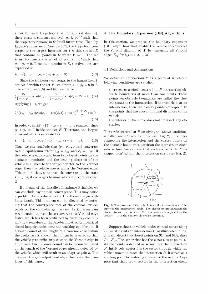
We define an intersection P as a point at which thefollowing conditions are satisfied:

– there exists a circle centered at P intersecting ob-stacle boundaries at more than two points. Thesepoints on obstacle boundaries are called the clos-

est points at the intersection. If the vehicle is at anintersection, then the closest points correspond tothe points that have local minimal distances to the

vehicle.– the interior of the circle does not intersect any ob-

stacles.

The circle centered at P satisfying the above conditionsis called an intersection circle (see Fig. 2). The linesconnecting the intersection and the closest points on

the obstacle boundaries partition the intersection circleinto sectors. We can see that each sector is the “pie-shaped area” within the intersection circle (see Fig. 2).

sector 3 sector 2

sector 0

∂Oj

Psector 1

∂Oi

blocked sector

Fig. 2 The position of the vehicle is at the intersection P . The

circle is the intersection circle. The closest points partition thecircle into sectors. For i = 1, 2, 3, the sector i is adjacent to thesector i− 1 in the counter-clockwise direction.

Suppose that the vehicle under control moves alongEij until it visits an intersection P , as illustrated in Fig.

2. It will detect two closest points on ∂Oi and ∂Oj , sinceP ∈ Eij . The sector that has these two closest points asits end points is defined as sector 0 for the intersection

P . Intuitively, sector 0 is the sector through which thevehicle moves to reach the intersection P . It serves as astarting point for indexing the rest of the sectors. Sup-

pose that there are n sectors in the intersection circle,

5

as seen in Fig. 2. Looking into the page, we then in-

dex the sectors in the counter-clockwise direction fromsector 0. The index k satisfies 0 ≤ k ≤ n− 1.

When two end points of a particular sector are onthe same obstacle, the sector is called a blocked sector,

which is illustrated as “sector 2” in Fig. 2. An opensector, illustrated as “sector 1” and “sector 3” in Fig.2, denotes a sector that is neither a blocked sector nor

a sector 0. If the intersection detected by the vehiclehas an open sector that has not been visited by thevehicle, then the intersection is marked as unexplored.

Otherwise, the intersection is marked as explored.

The following assumptions are made about theworkspace and the capability of the vehicle.

(A1) ∂V (Oi) is a simple closed curve for each Oi ∈ SO.In other words, ∂V (Oi) is continuous and no self-intersection occurs.

(A2) there are finitely many intersections inW . All blockedsectors for these intersections are detectable by thevehicle2.

(A3)∪

Oi∈SOV (Oi) = W.

(A4) the initial position of the vehicle is such that anobstacle other than OM is detected to the right ofthe vehicle3. The vehicle can distinguish OM from

other obstacles4.

We call a closed loop that contains intersections con-

nected by Voronoi edges an enclosing boundary if thereis no unexplored intersection strictly inside such a loopand the loop has no self-intersection. At any moment in

the BE algorithms, the enclosing boundary is unique.

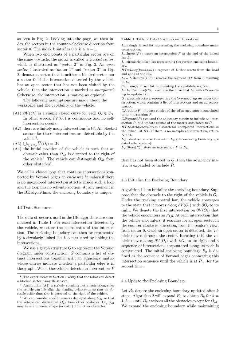
4.2 Data Structures

The data structures used in the BE algorithms are sum-marized in Table 1. For each intersection detected by

the vehicle, we store the coordinates of the intersec-tion. The enclosing boundary can then be representedby a circularly linked list L constructed by linking the

intersections.

We use a graph structure G to represent the Voronoidiagram under construction. G contains a list of dis-tinct intersections together with an adjacency matrix

whose entries indicate whether a particular edge is inthe graph. When the vehicle detects an intersection P

2 The experiments in Section 7 verify that the robot can detecta blocked sector using IR sensors.

3 Assumption (A4) is strictly speaking not a restriction, sincethe vehicle can initialize the heading orientation so that an ob-stacle other than OM is detected to the right of the vehicle.

4 We can consider specific sensors deployed along OM so thatthe vehicle can distinguish OM from other obstacles. Or, OM

may have a different shape (or color) from other obstacles.

Table 1 Table of Data Structures and Operations

Lu : singly linked list representing the enclosing boundary under

construction.Lu.Insert(P ) : insert an intersection P at the end of the linkedlist Lu.L : circularly linked list representing the current enclosing bound-ary.HT=L.seg(head,tail) : segment of L that starts from the headand ends at the tail.

Lr= L.Remove(HT ) : remove the segment HT from L resultingin Lr.CS : singly linked list representing the candidate segment.L=Lr.Combine(CS) : combine the linked list Lr with CS result-

ing in updated L.G : graph structure, representing the Voronoi diagram under con-struction, which contains a list of intersections and an adjacencymatrix.

G.Update(P ) : update entries of the adjacency matrix associatedto an intersection P .G.Expand(P ) : expand the adjacency matrix to include an inter-section P , and update entries of the matrix associated to P .

HT .Search(unexplored) : search for unexplored intersections inthe linked list HT . If there is no unexplored intersection, returnNULL.

Dk : disabled intersection set of Bk (the enclosing boundary up-dated after k steps).Dk.Store(P ) : store an intersection P in Dk.

that has not been stored in G, then the adjacency ma-trix is expanded to include P .

4.3 Initialize the Enclosing Boundary

Algorithm 1 is to initialize the enclosing boundary. Sup-pose that the obstacle to the right of the vehicle is Oi.

Under the tracking control law, the vehicle convergesto the state that it moves along ∂V (Oi) with ∂Oi to itsright. We denote the first intersection on ∂V (Oi) that

the vehicle encounters as P1,0. At each intersection thatthe vehicle encounters, it searches for an open sector inthe counter-clockwise direction, from the reader’s view,

from sector 0. Once an open sector is detected, the ve-hicle moves through the sector. Iterating this, the ve-hicle moves along ∂V (Oi) with ∂Oi to its right and a

sequence of intersections encountered along its path isconstructed. The initial enclosing boundary B0 is de-fined as the sequence of Voronoi edges connecting this

intersection sequence until the vehicle is at P1,0 for thesecond time.

4.4 Update the Enclosing Boundary

Let Bk denote the enclosing boundary updated after ksteps. Algorithm 2 will expand B0 to obtain Bk for k =1, 2, ... until Bk encloses all the obstacles except for OM .

We expand the enclosing boundary while maintaining

6

Algorithm 1 Construct the Initial Enclosing Bound-ary

i← 1.repeat

The vehicle encounters an intersection.Pi,0 ← the intersection.Search for an open sector in the counter-clockwise directionfrom sector 0. The vehicle moves through the first open sec-

tor.Pi,0.pointer ← first open sector.

if Pi,0 has an open sector that has not been visited by the

vehicle thenPi,0.mark ← unexplored.

else

Pi,0.mark ← explored.end ifLu.Insert(Pi,0).if Pi,0 ∈ G then

G.Update(Pi,0).else

G.Expand(Pi,0).end if

i← i+ 1.until the vehicle encounters P1,0 for the second time.L← Lu.

it as a simple closed curve tracked by the vehicle in the

clockwise direction.The boundary expansion is guaranteed by two rules,

called the sector selection rules, that decide which sec-

tor the vehicle should move through at an intersectionand when to update the enclosing boundary.

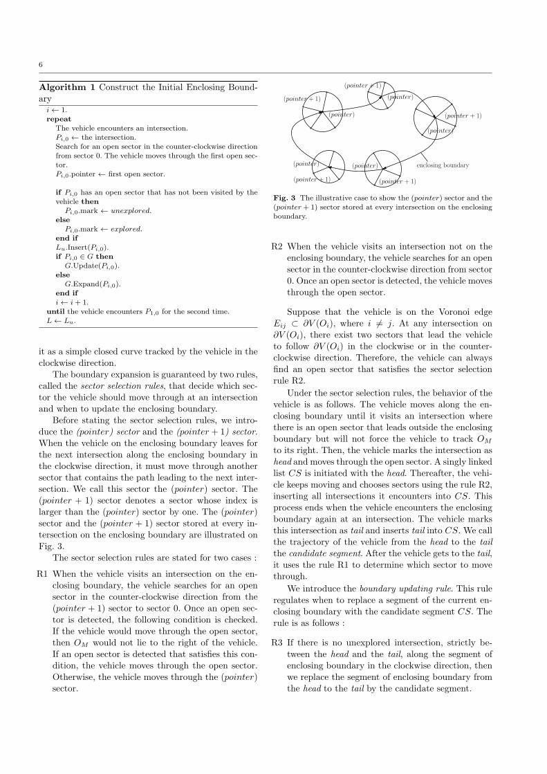
Before stating the sector selection rules, we intro-duce the (pointer) sector and the (pointer + 1) sector.

When the vehicle on the enclosing boundary leaves forthe next intersection along the enclosing boundary inthe clockwise direction, it must move through another

sector that contains the path leading to the next inter-section. We call this sector the (pointer) sector. The(pointer + 1) sector denotes a sector whose index is

larger than the (pointer) sector by one. The (pointer)sector and the (pointer + 1) sector stored at every in-tersection on the enclosing boundary are illustrated on

Fig. 3.The sector selection rules are stated for two cases :

R1 When the vehicle visits an intersection on the en-

closing boundary, the vehicle searches for an opensector in the counter-clockwise direction from the(pointer + 1) sector to sector 0. Once an open sec-

tor is detected, the following condition is checked.If the vehicle would move through the open sector,then OM would not lie to the right of the vehicle.

If an open sector is detected that satisfies this con-dition, the vehicle moves through the open sector.Otherwise, the vehicle moves through the (pointer)

sector.

enclosing boundary

(pointer)

(pointer + 1) (pointer)

(pointer)

(pointer)(pointer)

(pointer + 1)

(pointer + 1)

(pointer + 1)(pointer + 1)

Fig. 3 The illustrative case to show the (pointer) sector and the(pointer+ 1) sector stored at every intersection on the enclosingboundary.

R2 When the vehicle visits an intersection not on theenclosing boundary, the vehicle searches for an opensector in the counter-clockwise direction from sector

0. Once an open sector is detected, the vehicle movesthrough the open sector.

Suppose that the vehicle is on the Voronoi edgeEij ⊂ ∂V (Oi), where i = j. At any intersection on

∂V (Oi), there exist two sectors that lead the vehicleto follow ∂V (Oi) in the clockwise or in the counter-clockwise direction. Therefore, the vehicle can always

find an open sector that satisfies the sector selectionrule R2.

Under the sector selection rules, the behavior of thevehicle is as follows. The vehicle moves along the en-closing boundary until it visits an intersection where

there is an open sector that leads outside the enclosingboundary but will not force the vehicle to track OM

to its right. Then, the vehicle marks the intersection as

head and moves through the open sector. A singly linkedlist CS is initiated with the head. Thereafter, the vehi-cle keeps moving and chooses sectors using the rule R2,

inserting all intersections it encounters into CS. Thisprocess ends when the vehicle encounters the enclosingboundary again at an intersection. The vehicle marks

this intersection as tail and inserts tail into CS. We callthe trajectory of the vehicle from the head to the tailthe candidate segment. After the vehicle gets to the tail,

it uses the rule R1 to determine which sector to movethrough.

We introduce the boundary updating rule. This rule

regulates when to replace a segment of the current en-closing boundary with the candidate segment CS. Therule is as follows :

R3 If there is no unexplored intersection, strictly be-

tween the head and the tail, along the segment ofenclosing boundary in the clockwise direction, thenwe replace the segment of enclosing boundary from

the head to the tail by the candidate segment.

7

Suppose the current enclosing boundary is Bk. Fig-

ure 4 illustrates the case where the boundary updatingrule is satisfied. In this case, we update Bk by replac-ing the segment of enclosing boundary that starts from

the head and ends at the tail by the candidate segment.Figure 5 shows the update of L, the data structure ofthe enclosing boundary, when the boundary updating

rule is satisfied.

obstacle

head

tail

Bk

candidate segment

Fig. 4 The illustrative case where the enclosing boundary canbe expanded.

head tail

head tail

CS

L

explored

replace

Fig. 5 Update of the circularly linked list associated with bound-ary expansion.

Figure 6 shows one case where the boundary up-

dating rule is not satisfied. The dotted curve indicatesthe unexplored Voronoi edge. There are two unexploredintersections along the segment of enclosing boundary

from the head to the tail. If the rule for updating Bk

is not satisfied, as illustrated in Fig. 6, then we keepthe enclosing boundary unchanged. To prevent the ve-

hicle from repeatedly traversing the candidate segmentthat does not lead to boundary updates, the head ofsuch a candidate segment is recorded as a disabled in-

tersection in a set Dk that is associated with Bk. If thevehicle encounters a disabled intersection, it will ignorethis intersection and move along Bk to the next inter-

section.

Algorithm 2 Boundary ExpansionN denotes the number of intersections on the circularly linked

list L. Label the intersections on L in the clockwise directionas P1,0,P2,0,...,PN,0. i← 1 and k ← 0.while there is an obstacle other than OM outside the enclosingboundary do

The vehicle visits Pi,k on L.if Pi,k /∈ Dk and there exists an open sector, satisfyingthe sector selection rule R1, outside the enclosing bound-ary then

m← 1. E1 ← Pi,k. MeetTail← 0.while MeetTail = 1 do

The vehicle finds Em.if m == 1 then

Move through the open sector selected using the ruleR1.

else

Search for an open sector satisfying the rule R2, andmove through the selected open sector.

end ifEm.pointer← selected sector.

if Em has an open sector that has not been visited bythe vehicle then

Em.mark ← unexplored.else

Em.mark← explored.end ifCS.Insert(Em).if Em ∈ G then

G.Update(Em).else

G.Expand(Em).

end ifif m = 1 and the vehicle intersects L then

n← 1.while Em = Pn,k do

n← n+ 1.end whileT ← n and MeetTail← 1.

else

m← m+ 1.end if

end whilehead← E1 and tail← PT,k.

HT=L.seg(head,tail).if HT = NULL and HT .Search(unexplored)⊂ (head,tail) then

Lr=L.Remove(HT ).

L=Lr.Combine(CS).N denotes the number of intersections on L.P1,k+1 ← tail. Relabel the intersections on L in the

clockwise direction as P1,k+1,P2,k+1,...,PN,k+1.i← 1 and k ← k + 1.

elseDk.Store(head). i← T .

end ifelse

i← i+ 1.end if

if i > N theni← i−N .

end ifend while

8

obstacle

headtail

Bk

candidate segment

unexplored intersections

Fig. 6 The illustrative case where boundary expansion is notperformed according to the boundary updating rule R3.

5 Convergence of the BE algorithms

In this section, we prove the convergence of the bound-ary expansion algorithms, i.e., both Algorithm 1 andAlgorithm 2.

Lemma 1 Consider the vehicle and the workspace Wsatisfying assumptions (A1)-(A4). Suppose that the ob-

stacle to the right of the vehicle is Oi. Then, using Al-gorithm 1, the vehicle moves along ∂V (Oi) with ∂Oi

to its right and a sequence of intersections encountered

along its path is constructed. Algorithm 1 terminateswhen the vehicle returns to the first intersection in thesequence.

Proof : Suppose that the obstacle to the right of the ve-

hicle is Oi. Under the control law, the vehicle convergesto the state that it moves along ∂V (Oi) with ∂Oi to itsright. We denote the first intersection on ∂V (Oi) that

the vehicle encounters as P1,0, and label the intersec-tions the vehicle will encounter if it follows ∂V (Oi) with∂Oi to its right as (P1,0, P2,0, ..., Pn,0). We organize our

proofs in two steps:

1. Show that the vehicle moves to P2,0.2. Show that the vehicle visits P2,0 → P3,0... → Pn,0 →

P1,0.

1. For convenience, we call the closest point on ∂Oi as

C∂Oi . At P1,0, C∂Oi is to the right of the vehicle. Sup-pose that there are n sectors at P1,0. Sector 0 and sectorn− 1 have the common closest point at C∂Oi . The ve-

hicle moves through the sector n−1 if it is not blocked.If sector n− 1 is blocked, then the sector selection ruleR2 is applied so that the vehicle moves through the

next open sector having C∂Oi to the right of the vehi-cle. Therefore, the vehicle tracks ∂V (Oi) with ∂Oi toits right and will encounter P2,0.

2. Consider the case where the vehicle visits Pk,0 start-ing from Pk−1,0 for all 2 ≤ k ≤ n. Similar to step1, using the sector selection rule R2, the vehicle moves

along ∂V (Oi) with ∂Oi to its right until it visits Pk+1,0.By induction, if the vehicle uses the sector selection

rule R2 at P1,0, P2,0, ...Pn,0, then it visits the intersec-

tions following the sequence P1,0 → P2,0... → Pn,0 →

P1,0. Algorithm 1 ends when the vehicle returns to P1,0.

⊓⊔

To state Theorem 2, we need to introduce a few newnotations : Let Q denote an obstacle, other than OM ,outside Bk such that Bk

∩V (Q) = ∅. If Q is such that

Bk

∩V (Q) is a connected edge segment of Bk, then we

call it an addable obstacle Qk. Other than this possibil-ity based on the assumption that the boundary of every

Voronoi cell is a simple loop without self-intersection,there are only two more possibilities that Q can have.Let Qt denote an obstacle that Bk

∩V (Qt) is an inter-

section. Qd denotes an obstacle such that Bk

∩V (Qd)

is composed of disjoint edge segments or intersectionsof Bk. V (Qt), V (Qd), and V (Qk) are illustrated in Fig.

7.

Bk

V (Qt)

Bk

V (Qd)

Bk

V (Qk)

head

tail

S

Fig. 7 Illustration of V (Qt), V (Qd), V (Qk), and S. Qk isaddable but Qd and Qt are not addable.

Theorem 2 Consider the vehicle and the workspace W

satisfying assumptions (A1)-(A4). The vehicle exploresW using Algorithm 2. As long as there exists an obsta-cle other than OM outside the enclosing boundary Bk,

the following assertions hold :

1. Bk is a simple closed curve traversed in the clock-wise direction, and there is no unexplored intersec-

tion strictly inside Bk.2. There exists an addable obstacle Qk such that the

vehicle will move along a path CS ⊂ ∂V (Qk), but

CS = ∂V (Qk)∩Bk. The path CS intersects Bk at

two intersections that can be marked as head andtail. Further, CS is the candidate segment satisfying

the rule R3 for updating Bk.3. Bk will be expanded so that the obstacle Qk will be

inside the expanded enclosing boundary Bk+1.

Proof : Using Algorithm 1, the vehicle moves along∂V (Oi) with ∂Oi to its right and a sequence of inter-sections encountered along its path is constructed ac-

cording to Lemma 1. Therefore, B0 is in the clockwise

9

direction from the reader’s viewpoint, which is identical

to ∂V (Oi). Here, B0 = ∂V (Oi) is a simple closed curveusing assumption (A1). Furthermore, no intersection isstrictly inside B0.

We prove by induction. Suppose that Bk is a simpleclosed curve in the clockwise direction and that there

exists an obstacle other than OM outside Bk. Supposethat there is no unexplored intersection strictly insideBk. Now, we organize our proofs in four steps:

1. show that there exists an addable obstacle Qk as

long as there exists an obstacle other than OM out-side Bk.

2. show that there exists no unexplored intersectionstrictly between the starting intersection (head) and

the ending intersection (tail) of ∂V (Qk)∩

Bk.3. show that the vehicle moves along the path CS ⊂

∂V (Qk) and that the path intersects Bk at the start-

ing and the ending intersections of ∂V (Qk)∩Bk.

4. show that, after new enclosing boundary Bk+1 isgenerated,Qk is inside Bk+1. Bk+1 is a simple closed

curve traversed by the vehicle in the clockwise direc-tion, and there is no unexplored intersection strictlyinside Bk+1.

1. First, we show that there exists Q as long as there is

an obstacle other than OM outside Bk. Suppose that allobstacles Oi outside Bk are such that Bk

∩V (Oi) = ∅.

Then, since ∂V (OM ) should enclose both Bk and Oi,

∂V (OM ) has self-intersection.

Next, we prove the existence of Qk by contradic-

tion. Suppose all Q are either Qd or Qt. We first arguethat Qd must exist. If only Qt exists, then ∂V (OM ) hasself-intersection, since ∂V (OM ) should enclose both Bk

and Qt. For Qd, call the disjoint boundary segments asBk

∩V (Qd). Along Bk, there exist one or more edge

segments of Bk connecting these disjoint boundary seg-

ments. We select one segment S such that S and someedges of ∂V (Qd) form a closed loop that does not en-close Qd. S is illustrated in Fig. 7. This closed loop

can be constructed as a simple closed curve, since self-intersection occurs along neither ∂V (Qd) nor S ⊂ Bk.If S intersects ∂V (Qd) at more than two points, we can

always select a shorter segment of S so that a simpleclosed loop can be constructed. We call this closed loopQd

1. Inside the closed loop Qdi , we iteratively find an-

other loop for Qdi+1 until no more Qd

i+1 exists. Voronoiedges in S that exist along the inner most loop belongto neither V (Qd) nor V (Qt) for any Qt, which implies

that there exists an addable obstacleQk inside the innermost loop. Therefore, by contradiction, there exists anaddable obstacle Qk as long as there exists an obstacle

other than OM outside Bk.

2. We prove by contradiction. Suppose that an unex-

plored intersection exists strictly between the startingand the ending intersections of ∂V (Qk)

∩Bk. Then there

exists an unvisited Voronoi edge meeting the unexplored

intersection. Since we suppose that no unexplored in-tersection is strictly inside Bk, this unvisited Voronoiedge leads outside of the enclosing boundary toward

Qk, as illustrated in Fig. 8. Hence, at this unexploredintersection, three edges of ∂V (Qk) meet, resulting inself-intersection of ∂V (Qk). This is a contradiction to

assumption (A1).

edge ⊂ ∂V (Qk)

∂V (Qk)⋂Bk ⊂ ∂V (Qk)

Qk

unexplored

Fig. 8 Three edges of ∂V (Qk) meet at an unexplored intersec-tion on ∂V (Qk)

∩Bk. This is impossible, since we assume that

the boundary of each Voronoi cell is a simple closed curve.

3. We suppose that the vehicle has tracked Bk in theclockwise direction until it visits the starting intersec-

tion of ∂V (Qk)∩Bk. Then, we mark the starting in-

tersection as head and mark the ending intersection of∂V (Qk)

∩Bk as tail. Note that the direction of ∂V (Qk)∩

Bk is from the head to the tail, since Bk is in theclockwise direction.

When the vehicle visits the head, there exists an

open sector outside the enclosing boundary, as illus-trated in Fig. 7. Then, according to the rule R1, thevehicle moves through the open sector outside the en-

closing boundary with Qk to the vehicle’s right. There-after, it chooses sectors using the rule R2 and movesalong Voronoi edges.

We label the intersections the vehicle encounters if it

follows ∂V (Qk) with Qk to its right as (E1 = head , E2,..., En = tail). Similar to the proof of Lemma 1, thevehicle starting from Em moves along ∂V (Qk) with Qk

to its right until it visits Em+1. The sequence of Voronoiedges connecting the intersection sequence (E1 = head , E2,..., En = tail) is defined as the candidate segment CS ⊂∂V (Qk).

4. The boundary updating rule for Bk is satisfied. Thus,we update Bk by substituting ∂V (Qk)

∩Bk for CS.

There is no unexplored intersection strictly inside Bk+1,because there exists no unexplored intersection strictlybetween the starting and the ending intersections of

∂V (Qk)∩Bk.

10

We now prove that Bk+1 is a simple closed curve

in the clockwise direction. Since self-intersection of CScan not occur as we substitute ∂V (Qk)

∩Bk for CS,

Bk+1 is a simple closed curve. In addition, the direction

of Bk+1 is in the clockwise direction, since the directionof ∂V (Qk)

∩Bk is the same as that of CS.

Next, since CS∪(∂V (Qk)

∩Bk) ⊂ ∂V (Qk) is a

simple closed curve, CS∪(∂V (Qk)

∩Bk) = ∂V (Qk).

After we generate Bk+1, the area enclosed by CS∪

(∂V (Qk)∩Bk) is inside Bk+1, i.e., Q

k is inside Bk+1.

We have proved all the statements in Theorem 2. ⊓⊔

Corollary 1 Under Algorithms 1 and 2, the enclos-ing boundary converges in finite time to the state that

there is no obstacle other than OM outside the enclosingboundary.

Proof : As long as there is an obstacle other than OM

outsideBk, we can generateBk+1 using Theorem 2. Theprocess ends when there is no obstacle other than OM

outside Bk. Since there are finite number of obstacles,the process terminates in finite time.⊓⊔

Corollary 2 When Algorithm 2 terminates, a complete

Voronoi diagram is constructed for W .

Proof : When Algorithm 2 terminates, there is no un-

explored intersection outside the final enclosing bound-ary, since there is only OM outside. And, according toTheorem 2, there is no unexplored intersection strictly

inside the enclosing boundary either. Thus, all the in-tersections in W are explored. This implies that all theVoronoi edges in W are visited by the vehicle. Con-

sequently, the trajectory of the vehicle depicts all theVoronoi edges in W and a complete Voronoi diagram isconstructed. ⊓⊔

6 Performance Analysis

In this section, we provide an analytical upper boundfor the total time spent to construct Voronoi diagrams

in a regularized workspace. As the number of Voronoicells in a bounded workspace increases, each Voronoicell approaches to hexagonal shape [13, 27]. Thus, we

analyze the performance of the BE algorithms in theworkspace where each cell has a hexagonal shape withidentical size. Hexagonal Voronoi cells can be built us-

ing identical circular obstacles, as illustrated in Fig. 9.

Theorem 3 Consider a unit speed vehicle and a workspace

W with assumptions (A1)-(A4) satisfied. Suppose thatthere are M obstacles such that all obstacles, exceptfor OM , have hexagonal Voronoi cells with identical

size. Using the BE algorithms, the exploration time is

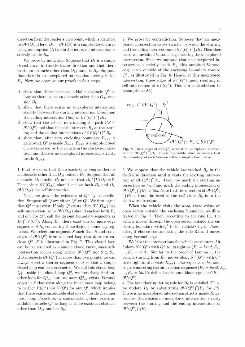
B5

OM

Fig. 9 A workspace where all Voronoi cells, except for V (OM ),have hexagonal shapes with identical size. Inside B5, there are 6obstacles.

bounded above by T ( 12M2 − 1

2M) where T denotes thetime for the vehicle to traverse along the edges of one

hexagonal Voronoi cell.

Proof : Consider the time to build B0. Since there isonly one Voronoi cell inside B0, the time to constructB0 is

TB0 = T. (17)

Next, consider the time to generate Bk+1 from Bk

where k ≥ 0. Suppose that Bk is generated and thatthe vehicle is at the tail of the candidate segment (CS)for generating Bk.

Using Theorem 2, at least one of the Voronoi cells,which is outside Bk and intersects the perimeter of Bk,is an addable obstacle Qk. This addable obstacle Qk

will be an obstacle that is inside Bk+1. The vehicle

moves along Bk to reach the starting intersection (head)of ∂V (Qk)

∩Bk. The vehicle’s maximal traversal dis-

tance to meet the starting intersection of ∂V (Qk)∩Bk

is bounded above by the length of Bk. Note that thevehicle has unit speed and that the number of Voronoicells, which are inside Bk, is k+1. Therefore, the length

of Bk is bounded above by (k + 1)T . In addition, thelength of CS, which connects the starting and the end-ing intersections of ∂V (Qk)

∩Bk, is bounded above by

T . Hence, we derive the time to construct Bk+1 as

TBk+1≤ TBk

+ (k + 1)T + T, (18)

where TBkdenotes the time to constructBk. Using (18),

we obtain

TBk≤ T ( 12k

2 + 32k + 1), (19)

since TB0 = T (see (17)). There are k+1 and M−1 ob-stacles inside Bk and ∂V (OM ) respectively. Therefore,

our algorithms terminate when

k + 1 = M − 1. (20)

11

Hence, replacing k in (19) by M − 2, we obtain the

upper bound on time for the construction of Voronoidiagrams using the BE algorithms as

Tc ≤ T (1

2M2 − 1

2M). (21)

Therefore, the expected construction time is on the or-

der of M2. ⊓⊔

7 Simulation and Experimental Results

We introduce two strategies to improve the time effi-

ciency of the BE algorithms. Both the improved BEalgorithms and the feedback control law (11) are im-plemented in MATLAB simulations. We also perform

MATLAB simulations of the exploration algorithms andthe control law in [10] to compare with the BE algo-rithms. We then present the experimental results on a

Khepera III robot in an environment with three obsta-cles.

7.1 Simulation Results

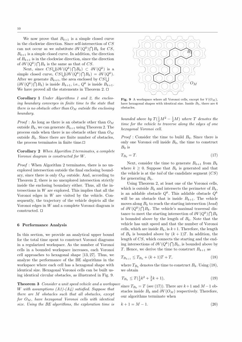
Figure 10 depicts the MATLAB simulation results usingthe exploration algorithms and the control law in [10],

and Fig. 11 depicts the results using the BE algorithmsand the control law. In both Fig. 10 and Fig. 11, theinitial position of the vehicle is (2, 20), and the obstacle

boundaries are shown in thick red curves. The trajec-tory of the vehicle is plotted with blue points. Along thevehicle’s trajectory, the intersections are marked withlarge green dots.

In [10] and related works, the vehicle moves through

a sector to check whether the sector is open or blocked.In other words, the vehicle moves through a blockedsector until it detects a blocking obstacle boundary. Our

simulation results show that 63.4 time unit is spent tofinish the exploration in Fig. 10.

The BE algorithms are theoretically sound, but wecan improve the time efficiency of the algorithms with-

out violating the correctness of the algorithms. We haveimplemented two strategies. The first strategy is in-spired by the fact that the vehicle does not have to

traverse the entire enclosing boundary to find an unex-plored intersection. Whenever the vehicle finishes build-ing a candidate segment, it plans the shortest path to

reach the nearest unexplored intersection on the enclos-ing boundary. Once the vehicle reaches the unexploredintersection, it branches out of the loop to expand the

enclosing boundary.

0 10 20 30 40 500

5

10

15

20

25

30

35

40

45

50

x

y

Fig. 10 The Voronoi diagram constructed by the vehicle using

the exploration algorithms and the control law in [10].

The second strategy is to store the candidate seg-ment with a disabled intersection, as discussed in Sec-

tion 4.4. If the boundary updating rule is not satis-fied, we store the corresponding candidate segment asa disabled candidate segment. Whenever the enclosing

boundary is updated, the vehicle checks the disabledcandidate segment to see whether there is still an unex-plored intersection from the head to the tail. If no unex-

plored intersection is found, then the disabled candidatesegment will be enabled and boundary expansion canbe performed using this candidate segment. This strat-

egy updates the enclosing boundary without letting thevehicle traverse the disabled candidate segment again.

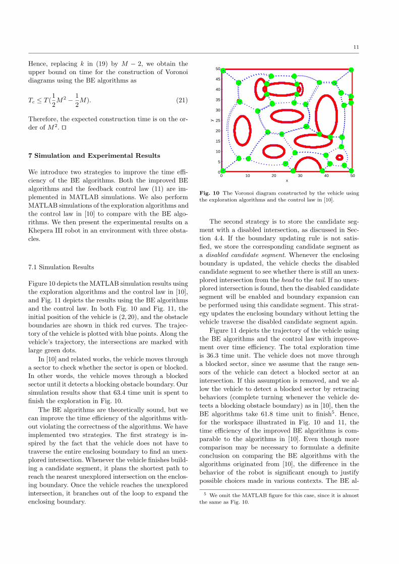
Figure 11 depicts the trajectory of the vehicle usingthe BE algorithms and the control law with improve-ment over time efficiency. The total exploration time

is 36.3 time unit. The vehicle does not move througha blocked sector, since we assume that the range sen-sors of the vehicle can detect a blocked sector at an

intersection. If this assumption is removed, and we al-low the vehicle to detect a blocked sector by retracingbehaviors (complete turning whenever the vehicle de-

tects a blocking obstacle boundary) as in [10], then theBE algorithms take 61.8 time unit to finish5. Hence,for the workspace illustrated in Fig. 10 and 11, the

time efficiency of the improved BE algorithms is com-parable to the algorithms in [10]. Even though morecomparison may be necessary to formulate a definite

conclusion on comparing the BE algorithms with thealgorithms originated from [10], the difference in thebehavior of the robot is significant enough to justify

possible choices made in various contexts. The BE al-

5 We omit the MATLAB figure for this case, since it is almost

the same as Fig. 10.

12

gorithms have added an option to the library of explo-

ration algorithms.

0 10 20 30 40 500

5

10

15

20

25

30

35

40

45

50

x

y

Fig. 11 The Voronoi diagram constructed by the BE algorithmsand the underlying control law.

7.2 Experimental Results

The validity of our algorithms and the control law (11)is verified using a miniature robot Khepera III [25] that

localizes itself based on an odometry system. The Khep-era III robot has nine IR sensors and five sonar sensors.In the experiments, we use only IR sensors for range

measurements.

As the robot maneuvers in the workspace, a MAT-

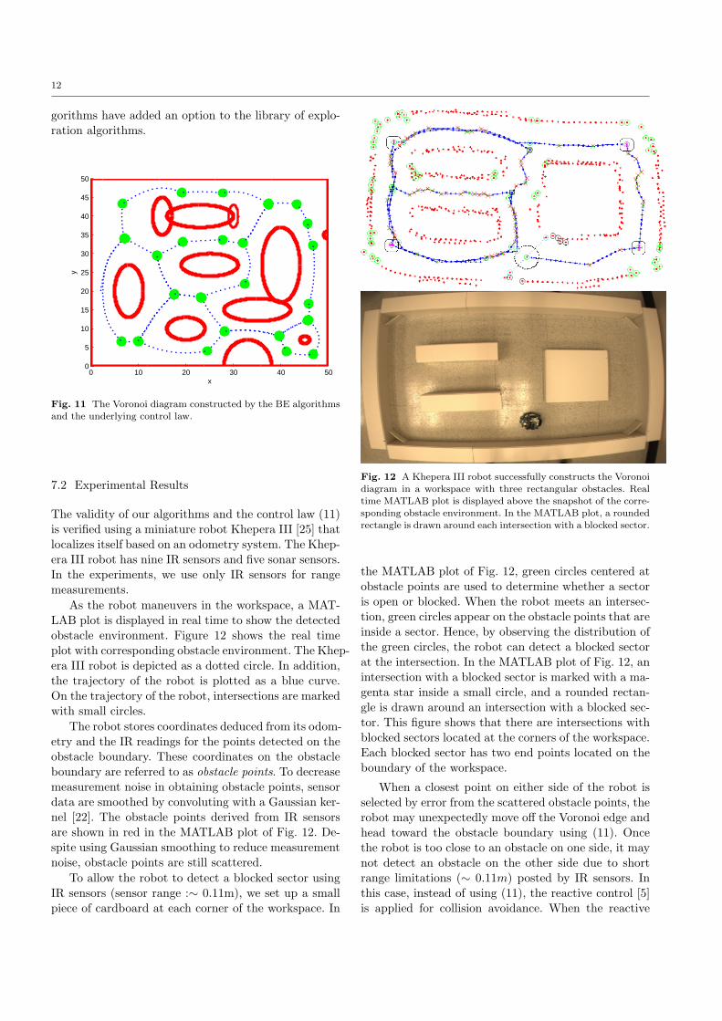
LAB plot is displayed in real time to show the detectedobstacle environment. Figure 12 shows the real timeplot with corresponding obstacle environment. The Khep-

era III robot is depicted as a dotted circle. In addition,the trajectory of the robot is plotted as a blue curve.On the trajectory of the robot, intersections are marked

with small circles.

The robot stores coordinates deduced from its odom-

etry and the IR readings for the points detected on theobstacle boundary. These coordinates on the obstacleboundary are referred to as obstacle points. To decrease

measurement noise in obtaining obstacle points, sensordata are smoothed by convoluting with a Gaussian ker-nel [22]. The obstacle points derived from IR sensors

are shown in red in the MATLAB plot of Fig. 12. De-spite using Gaussian smoothing to reduce measurementnoise, obstacle points are still scattered.

To allow the robot to detect a blocked sector usingIR sensors (sensor range :∼ 0.11m), we set up a small

piece of cardboard at each corner of the workspace. In

Fig. 12 A Khepera III robot successfully constructs the Voronoidiagram in a workspace with three rectangular obstacles. Real

time MATLAB plot is displayed above the snapshot of the corre-sponding obstacle environment. In the MATLAB plot, a roundedrectangle is drawn around each intersection with a blocked sector.

the MATLAB plot of Fig. 12, green circles centered atobstacle points are used to determine whether a sector

is open or blocked. When the robot meets an intersec-tion, green circles appear on the obstacle points that areinside a sector. Hence, by observing the distribution of

the green circles, the robot can detect a blocked sectorat the intersection. In the MATLAB plot of Fig. 12, anintersection with a blocked sector is marked with a ma-

genta star inside a small circle, and a rounded rectan-gle is drawn around an intersection with a blocked sec-tor. This figure shows that there are intersections with

blocked sectors located at the corners of the workspace.Each blocked sector has two end points located on theboundary of the workspace.

When a closest point on either side of the robot isselected by error from the scattered obstacle points, the

robot may unexpectedly move off the Voronoi edge andhead toward the obstacle boundary using (11). Oncethe robot is too close to an obstacle on one side, it may

not detect an obstacle on the other side due to shortrange limitations (∼ 0.11m) posted by IR sensors. Inthis case, instead of using (11), the reactive control [5]

is applied for collision avoidance. When the reactive

13

control is applied, the robot’s position is marked with

“×” in the MATLAB plot (Fig. 12).

In the case where the robot has to move along the

enclosing boundary that has been constructed previ-ously, the robot follows the enclosing boundary using amethod similar to those in [14, 18, 36]. First, we let a

virtual robot move along the enclosing boundary aheadof the real robot. Then, the real robot keeps moving to-ward the virtual robot to follow the enclosing boundary.

Using the virtual robot approach, the real robot buildsa smoother trajectory than the enclosing boundary ini-tially built. In addition, the real robot can follow the

enclosing boundary with higher speed, since the robotdoes not have to process sensor data while it movestoward the virtual robot.

8 Conclusions

In this paper, we develop a provably convergent controllaw that enables a vehicle to follow Voronoi edges usingrange sensors. We then develop the boundary expan-

sion algorithms so that the Voronoi diagram structureof an unknown compact area can be constructed in fi-nite time. The algorithms implement decisions based

on information gathered at each intersection that thevehicle encounters. We prove that such local decisionsresult in a global behavior that leads to the construction

of a complete Voronoi diagram in finite time. Further-more, we provide an analytic upper bound for the totaltime spent to construct Voronoi diagrams in a regu-

larized workspace. Simulation and experimental resultsare provided to demonstrate the effectiveness of boththe control law and the exploration algorithms.

Acknowledgements We greatly appreciate Sean Maxon for hisassistance in setting up the experiments and analyzing data.We thank Justin Shapiro for preparing the Khepera III robots.

The research is supported by ONR grants N00014-08-1-1007 andN00014-09-1-1074, and NSF grants ECCS-0845333(CAREER) andCNS-0931576.

References

1. Ahn S, Doh NL, Chung W, Nam S (2008) The robust con-

struction of a generalized Voronoi graph (GVG) using partialrange data for guide robots. Industrial Robot: An InternationalJournal 35:259-265

2. Aurenhammer F (1991) Voronoi diagrams - a survey of a fun-damental geometric data structure. ACM Computing Surveys23:345-405

3. Bandyopadhyay S, Coyle EJ (2003) Minimizing communica-tion costs in hierarchically clustered networks of wireless sen-

sors. Wireless Communications and Networking 2:1274-1279

4. Bhattacharya P, Gavrilova ML (2008) Roadmap-based path

planning - using the Voronoi diagram for a clearance-based

shortest path. IEEE Robotics and Automation Magazine 15:58-66

5. Brooks RA (1999) Cambrian Intelligence: The Early History

of the New AI, MIT Press6. Brown G (1965) Point density in stems per acre. NewzealandForestry Service Research Notes 38:1-11

7. Choset H, Burdick J (2000) Sensor-based exploration: the hier-archical generalized Voronoi diagram. The International Jour-nal of Robotics Research 19:96-125

8. Choset H, Konukseven I, Burdick J (1996) Mobile robot navi-

gation: issues in implementating the generalized Voronoi graphin the plane. In Proc. of IEEE/SICE/RSJ International Con-ference on Multisensor Fusion and Integration for IntelligentSystems, Washington DC, USA, pp. 241-248

9. Choset H, Konukseven I, Rizzi A (1997) Sensor based plan-

ning: a control law for generating the generalized Voronoigraph. In Proc. of 8th International Conference on AdvancedRobotics, CA, USA, pp. 333-338

10. Choset H, Nagatani K (2001) Topological simultaneous local-ization and mapping (SLAM): toward exact localization with-

out explicit localization. IEEE Transactions on Robotics andAutomation 17:125-137

11. Choset H, Walker S, Eiamsa-Ard K, Burdick J (2000) In-cremental construction of the hierarchical generalized Voronoigraph. The International Journal of Robotics Research 19:126-

14812. Cortes J, Martınez S, Karatas T, Bullo F (2004) Coverage

control for mobile sensing networks. IEEE Transactions onRobotics and Automation 20(2):243-255

13. Du Q, Faber V, Gunzburger M (1999) Centroidal Voronoitessellations: applications and algorithms. SIAM Review41:637-676

14. Egerstedt M, Hu X, Stotsky A (2001) Control of mobile plat-

forms using a virtual vehicle approach. IEEE Transactions onAutomatic Control 46:1777-1782

15. Fortune SJ (1987) A sweepline algorithm for Voronoi dia-grams. Algorithmica 2:153-174

16. Garrido S, Moreno L, Blanco D, Martin F (2007) Exploratorynavigation based on Voronoi transform and fast marching. In

IEEE International Symposium on Intelligent Signal Process-ing, Xiamen, China, pp. 1-6

17. Khalil HK (2002) Nonlinear Systems (3rd ed), Prentice Hall18. Kim J, Zhang F, Egerstedt M (2009) Curve tracking controlfor autonomous vehicles with rigidly mounted range sensors.Journal of Intelligent and Robotic Systems 56:177-198

19. Klein R (1988) Abstract Voronoi diagrams and their applica-tions. Computational Geometry and its Applications 333:148-

15720. Klein R (1990) Concrete and Abstract Voronoi diagrams,Springer

21. Lavalle SM (2006) Planning Algorithms, Cambridge Univer-sity Press

22. Lindeberg T (1990) Scale-space for discrete signals. IEEETransactions of Pattern Analysis and Machine Intelligence

12(3):234-25423. Martınez S, Cortes J, Bullo F (2007) Motion coordination

with distributed information. IEEE Control Systems Magazine27(4):75-88

24. Mead R (1966) A relation between the individual plant-spacing and yield. Ann. of Bot., N. S. 30:301-309

25. Mondada F, Franzi E, Ienne P (1993) Mobile robot miniatur-isation: a tool for investigation in control algorithms. In Proc. of

the Third International Symposium on Experimental Robotics,Kyoto, Japan, pp. 501-513

26. Nagatani K, Choset H (1999) Toward robust sensor basedexploration by constructing reduced generalized Voronoi graph.In Proc. of IEEE/RSJ International Conference on Intelligent

Robots and Systems, Kyongju, Korea, pp. 1687-1692

14

27. Newman D (1982) The hexagon theorem. IEEE Transactionson Information Theory 28:137-139

28. Okabe A, Boots B, Sugihara K (1992) Spatial Tessellations:Concepts and Applications of Voronoi Diagrams, Wiley

29. Rao NSV, Stoltzfus N, Iyengar SS (1991) A retraction

method for learned navigation in unknown terrains for a cir-cular robot. IEEE Transactions on Robotics and Automation7:699-707

30. Reddy PV, Justh EW, Krishnaprasad PS (2006) Motion

camouflage in three dimensions. In Proc. of 45th IEEE Conf.on Decision and Control, San Diego, CA, USA, pp. 3327-3332

31. Samson C (1995) Control of chained systems: Application topath-following and time-varying point-stabilization of mobile

robots. IEEE Transactions on Automatic Control 40:64-7732. Sudha N, Nandi S, Sridharan K (1999) A parallel algorithmto construct Voronoi diagram and its VLSI architecture. InProc. of IEEE International Conference on Robotics and Au-

tomation, Detroit, MI, USA, pp. 1683-168833. Svec P (2007) Using methods of computational geometry inrobotics. PhD Thesis, Brno University of Technology, Brno,

Czech Republic34. Wein R, Berg JP, Halperin D (2005) The visibility–Voronoicomplex and its applications. In Proc. of the Twenty-first An-nual Symposium on Computational Geometry, Pisa, Italy, pp.

63-7235. Zhang F, Fratantoni DM, Paley D, Lund J, Leonard NE(2007) Control of coordinated patterns for ocean sampling. In-ternational Journal of Control 80:1186-1199

36. Zhang F, Justh E, Krishnaprasad PS (2004) Boundary fol-lowing using gyroscopic control. In Proc. of 43rd IEEE Conf.on Decision and Control, Atlantis, Paradise Island, Bahamas,pp. 5204-5209

37. Zhang F, Leonard NE (2007) Coordinated patterns of unitspeed particles on a closed curve. Systems and Control Letters56:397-407

38. Zhang F, O’Connor A, Luebke D, Krishnaprasad PS (2004)

Experimental study of curvature-based control laws for obstacleavoidance. In Proc. of IEEE International Conf. on Roboticsand Automation, New Orleans, LA, USA, pp. 3849-3854