Distributed Voronoi diagram computation in wireless sensor

networks

Waleed Alsalih(1) Kamrul Islam(1) Yurai Nunez-Rodrıguez(1) Henry Xiao(1)∗

(1)Queen’s University(waleed/islam/yurai/xiao@cs.queensu.ca)School of Computing, Queen’s University

Kingston, Ontario, Canada K7L 3N6

Abstract

We study the problem of computing Voronoi diagrams in the context of wireless sensornetworks. Sensors can be seen as points in the plane and the Voronoi diagram of a set ofsensors is a meaningful way of partitioning the plane such that each sensor is assigned theset of points that are closer to itself than to any other sensor. We present an algorithm tosolve this problem efficiently in a distributed fashion. To the best of our knowledge, this is thefirst non-trivial distributed algorithm that computes the complete Voronoi diagram. Existingalgorithms either produce inaccurate Voronoi diagrams [10] or Voronoi diagrams [1] of boundedregions. Furthermore, simulation results show that our algorithm uses a much smaller numberof transmissions and, therefore, is more efficient in terms of energy consumption.

Keywords: Sensor Networks, Voronoi diagram, Delaunay triangulation,convex hull, distributed algorithm, Computational Geometry

∗These authors (all students) have contributed equally to the work presented in this manuscript.

1 Introduction

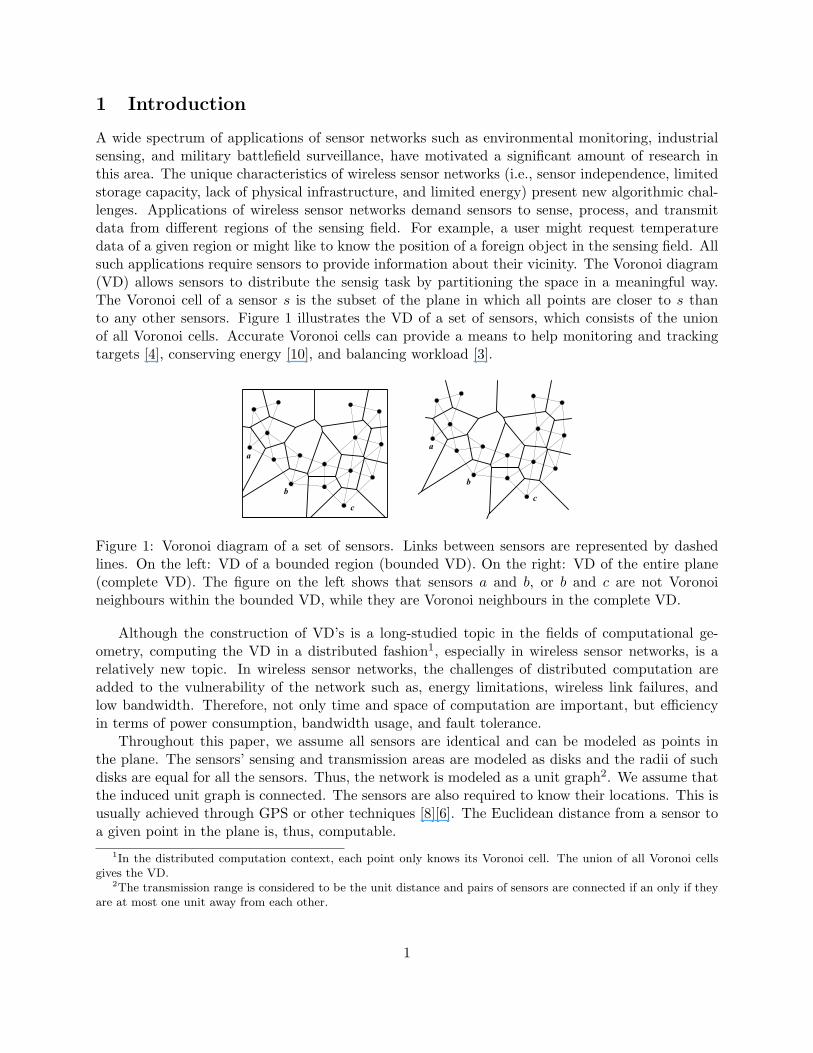
A wide spectrum of applications of sensor networks such as environmental monitoring, industrialsensing, and military battlefield surveillance, have motivated a significant amount of research inthis area. The unique characteristics of wireless sensor networks (i.e., sensor independence, limitedstorage capacity, lack of physical infrastructure, and limited energy) present new algorithmic chal-lenges. Applications of wireless sensor networks demand sensors to sense, process, and transmitdata from different regions of the sensing field. For example, a user might request temperaturedata of a given region or might like to know the position of a foreign object in the sensing field. Allsuch applications require sensors to provide information about their vicinity. The Voronoi diagram(VD) allows sensors to distribute the sensig task by partitioning the space in a meaningful way.The Voronoi cell of a sensor s is the subset of the plane in which all points are closer to s thanto any other sensors. Figure 1 illustrates the VD of a set of sensors, which consists of the unionof all Voronoi cells. Accurate Voronoi cells can provide a means to help monitoring and trackingtargets [4], conserving energy [10], and balancing workload [3].

a

b

c

a

b

c

a

b

c

a

b

c

Figure 1: Voronoi diagram of a set of sensors. Links between sensors are represented by dashedlines. On the left: VD of a bounded region (bounded VD). On the right: VD of the entire plane(complete VD). The figure on the left shows that sensors a and b, or b and c are not Voronoineighbours within the bounded VD, while they are Voronoi neighbours in the complete VD.

Although the construction of VD’s is a long-studied topic in the fields of computational ge-ometry, computing the VD in a distributed fashion1, especially in wireless sensor networks, is arelatively new topic. In wireless sensor networks, the challenges of distributed computation areadded to the vulnerability of the network such as, energy limitations, wireless link failures, andlow bandwidth. Therefore, not only time and space of computation are important, but efficiencyin terms of power consumption, bandwidth usage, and fault tolerance.

Throughout this paper, we assume all sensors are identical and can be modeled as points inthe plane. The sensors’ sensing and transmission areas are modeled as disks and the radii of suchdisks are equal for all the sensors. Thus, the network is modeled as a unit graph2. We assume thatthe induced unit graph is connected. The sensors are also required to know their locations. This isusually achieved through GPS or other techniques [8][6]. The Euclidean distance from a sensor toa given point in the plane is, thus, computable.

1In the distributed computation context, each point only knows its Voronoi cell. The union of all Voronoi cellsgives the VD.

2The transmission range is considered to be the unit distance and pairs of sensors are connected if an only if theyare at most one unit away from each other.

1

In the following section, we review previous approaches to computing the VD in wireless sensornetworks. In Section 3 we show that the bounded VD can be computed in a localized way undercertain assumptions. Then we discuss our main algorithm for the distrubuted computation of thecomplete VD where such assumptions are relaxed. The performance of our main algorithm isdiscussed in Section 4. Experimental results and a comparative analysis are provided in Section 5.

2 Previous works

For a given set of n points in the plane, it is known that the VD can be effectively computed inO(n log n) time in a centralized fashion (see Fortune’s algorithm for an example [5]). However, itis a harder problem to compute the VD of a set of sensors in a distributed way. The reason stemsfrom the fact that each sensor needs information about its neighbouring sensors to compute itsVoronoi cell, and in the worst case, a sensor needs to know all other sensors.

Zhou, Das, and Gupta proposed a k-hop algorithm. They achieved efficiency by limiting theneighbourhood of a sensor that is considered when computing its Voronoi cell: only neighboursthat are k hops away are considered [10]. Their algorithm does not always give the exact VD for aconstant k; however, it provides good approximations since most Voronoi neighbours are likely tobe nearby in the network.

Sharifzadeh and Shahabi provided a different way for each sensor to compute its Voronoi cell [9].In their algorithm, a sensor s discards a set of other sensors that clearly have no influence on itscurrent Voronoi cell. The decision whether another sensor (t) affects the Voronoi cell of s is basedon the position of t with respect to a circle centered at s, such that if t is located outside the circle,it is discarded by s. Unfortunately, these bounding circles could be relatively large at the beginningof the computation, which provides a poor bound on the area that contains the potential Voronoineighbours. Furthermore, the authors did not provide implementation details nor analysis of theirmethod.

More recently, Bash and Desnoyers designed an algorithm to compute the bounded VD (Fig-ure 1 (left)) utilizing the GPSR routing protocol [1]. The basic idea is to successively refine theapproximation to the Voronoi cells upon discovery of other sensors in the network. Given a sensor,s, the algorithm starts with the entire bounded region as the Voronoi cell of s. then, a message issent to each of the vertices of the current Voronoi cell using GPSR. A property of GPSR is thata message destined to a vertex will be delivered to the sensor that is the closest to this vertex.This process is referred to as probing. If a probe coming from s is delivered to a sensor t (i.e., tis the nearest sensor to the probed vertex), t replies to s and the current Voronoi cell of s will berefined with respect to t. No more probes are sent by s once it becomes the nearest sensor to all thevertices on its Voronoi cell. The authors also considered two local improvements to their originalalgorithm. First, the discovery of other sensors that influence the current Voronoi cell of a sensor(s) does not have to wait for the probe message to reach its destination. In fact, the first sensor (r)on the routing path that is closer to the probed vertex than s affects the current Voronoi cell of s.Thus r can reply to the sender without further forwarding the message. The second improvementcomes from the observation that Voronoi neighbours do not have to all probe the shared vertices.It is sufficient that one of the sensors probes such vertex and lets the others know about the result.This algorithm, including the two improvements, is referred to as BD07 throughout this paper.

In this work, we address several deficiencies of the algorithms reviewed above. Zhou, Das, andGupta’s algorithm [10] only computes an approximation of the exact Voronoi cells. Sharifzadeh

2

and Shahabi’s algorithm [9] may require global knowledge in the worst case. Their algorithm maybe suitable for scenarios with high sensor density. Bash and Desnoyers’ algorithm (BD07) [1] is notindependent of the routing protocol since it relies on GPSR. BD07 is also restricted to a boundedregion where the boundary (i.e., the vertices on the boundary) needs to be known by all sensors inthe area, or more critically, the boundary may be imprecise or fuzzy. Furthermore, the boundedVD does not contain the complete set of Voronoi vertices which results in topological informationoutside the bounded region not being known (see Figure 1 for an example). Notice that the completeVD would allow for straightforward computation of other useful topological structures such as theDelaunay triangulation and the convex hull.

Our goal is to compute the complete VD preserving the distributed fashion of computation ofthe VD without flooding the network. We present an algorithm that achieves this goal, and in fact,uses fewer transmissions to compute the VD than BD07. Presumably, our algorithm consumes lessenergy and is faster.

3 Distributed Voronoi diagram computation

In this section, we propose two distributed algorithms for computing the VD in wireless sensornetworks. For now, a sensor network defines a unit graph. Below, we generalize this model toinclude certain types of subgraphs of the unit graph. The sensors are assumed to be in a generalposition, that is, no three sensors are collinear and no four sensors fall on the same circle. Subsection3.1, presents a special type of network where assumptions are made regarding coverage, sensingrange, and transmission range. We show that this problem can be solved locally by just consideringthe immediate neighbours. In subsection 3.2, we deal with a more general problem in which suchassumptions are relaxed and the complete VD is constructed. For the more general problem, thesolution is distributed rather than localized. Localized solutions are not possible in this case sinceVoronoi neighbours can be as distant from each other as desired.

3.1 The bounded Voronoi diagram

Given a sensor network of k sensors placed in a convex region R, the bounded VD partitions theregion into k convex polygons that define the bounded Voronoi cells. A Delaunay edge between twosensors whose bounded Voronoi cells share an edge is called a bounded Delaunay edge.

Before discussing our claim on the bounded VD, we define the following terms.

- Sr is the sensing range of a sensor. A sensor can detect (i.e., sense) a signal if the distance tothe source is at most Sr.

- Tr is the transmission range of a sensor. Two sensors can communicate with each other if thedistance between them is at most Tr.

Theorem 3.1 If Tr ≥ 2Sr and all points in R are sensed by at least one sensor, the maximumlength of a Delaunay edge is Tr.

Proof We prove this theorem by contradiction. Assume that there is a bounded Delaunay edge(u, v), such that ‖u, v‖ > Tr, where ‖u, v‖ is the Euclidean distance between u and v. By definition,the points on the bounded Voronoi edge between u and v have u and v as their nearest sensors.However, since the bounded Voronoi edge is a segment of the bisector between u and v, the distance

3

between a point p on this Voronoi edge and u or v is at least ‖u, v‖/2. Therefore, ‖u, p‖ > Tr/2,‖v, p‖ > Tr/2 and ‖u, p‖ > Sr, ‖v, p‖ > Sr. This means that p is not covered which contradictsour assumption that all points in R are covered. 2

By Theorem 3.1, a bounded VD can be constructed locally: each sensor constructs its own cell onlyusing information about its immediate (one-hop) neighbours. The localized algorithm is describedbelow.

Algorithm 1: Localized algorithm for the Bounded Voronoi DiagramEvery sensor broadcasts its location to its neighboursEvery sensor u computes its own bounded Voronoi cell as the intersection

of the half spaces defined by the bisectors between u and each of itsneighbours, and the bounded sensing field

3.2 The complete Voronoi diagram

In practice, the ratio between the transmission and sensing ranges may not apply. Thus, algorithmsthat compute the complete VD in a more general scenario are needed. We propose a new algorithmfor distributedly computing the VD, namely the completely cooperative (CC) algorithm. The CCalgorithm is distributed in the sense that each sensor computes its own Voronoi cell. The taskof computing a Voronoi cell can be split into two main parts: finding the Voronoi neighboursof the sensor, and solving the geometric intersections of bisectors (between the sensor and itsneighbours). Even when these two parts are handled simultaneously, we will focus on the discoveryof the neighbours since the intersection of geometric primitives do not impose any new chanllenge.

The basic idea behind the CC algorithm is that sensors do not need to send out queries to thenetwork in order to discover their Voronoi neighbours; instead, sensors are informed about possibleVoronoi neighbours by other neighbours. In order to explain the details of the algorithm, we adoptthe following terminology. Let S be a set of sensors embedded in the plane and let G = (S, L) bethe connected unit graph induced by S, where L ⊆ S×S contains pairs of sensors that can directlycommunicate with each other. Let also V D(G) be the VD of G. We refer to an elements of L as alink, saving the term edge for the corresponding element in the VD. Similarly, we refer to sensorsthat share a link as adjacent and to sensors that share a Voronoi edge as neighbours.

We informally describe how the CC algorithm works before giving a more formal description.Let s be a sensor that receives a message about a new candidate for (Voronoi) neighbour (t) at somepoint during the computation. Then s proceeds to compute the intersection of the correspondinghalfplane, as defined by the bisector between itself and t, with its current cell C. We call this stepthe refinement of a cell. If the new cell C ′ resulting from the intersection is equal to C, t is discardedas a non-neighbour; otherwise (C ′ ⊂ C) t becomes a neighbour of s. In the latter case, new verticesappear on C ′ and some vertices of C fall outside of C ′. Figure 2 illustrates this stage of the process.Two adjacent vertices that fall outside of C ′, define a piece of bisector for a sensor t2 that is thendiscarded. A new vertex v on C ′ is created by the intersection of the bisector between s and t,and the bisector between a certain sensor t1 and s. Therefore, t and t1 may be neighbours of eachother since they have a common Voronoi vertex according to s’s cell. Consequently, s proceeds toinform both t and t1 about each other. This way, the information about possible neighbours flows

4

towards the corresponding sensors until every pair of neighbours find each other. See Theorem 3.2for the correctness of this approach. A pseudocode description of the CC algorithm is given below.

Figure 2: Succesive approximations (C and C ′) to the Voronoi cell of s. Thin dashed lines representlinks. The bisector b(s, t) between nodes s and t is represented with a thick dashed line. Vertexv appears on C ′ and indicates that s and t are neighbours and also that s should notify t and t1about each other. t2 is no longer a neighbour of s.

Initially, the cell of any sensor s is equal to the entire plane. Then all sensors broadcast theirlocations triggering the entire computation as explained above.

The following describes the most important terminology used in Algorithm 2. Let s be a sensorwith location s.loc, a field s.cell that stores the description of its Voronoi cell, and a message queues.q used for the computation. Let also s be equipped with methods s.refine(t.loc) that carries outthe refinements and s.send message(t1.loc, t2.loc) that sends a message to sensor t1 containing thelocation of t2. This results in t2.loc being added to the message queue of t1 (i.e. t1.q). Notice that acell may be bounded or unbounded and may or may not contain vertices. If s.cell contains verticesthese can be accessed through s.cell.verts. A vertex v of a Voronoi cell is defined as a point inthe plane equipped with a method v.third(s.loc, t.loc) that returns the location of the third sensorassociated to v that is neither s nor t.

Algorithm 2: Completely Cooperative (CC): Computes the Voronoi cell of each sensor.// Initialize the cells.cell = ENTIRE_SPACE// Broadcast the sensor location to all adjacent sensorss.send_message( BROADCAST, s.loc )// Process each (sensor) message in the queuewhile( t.loc = s.q.get_message )

old_Cell = s.cells.cell = s.cell.refine( t.loc )for each( v in s.cell.verts and not in old_Cell.verts )

// Notify each pair of possible neighbours about each others.send_message( t.loc, v.third_sensor( s.loc, t.loc ) )s.send_message( v.third_sensor( s.loc, t.loc ), t.loc )

endend

5

Theorem 3.2 Let G be the induced unit graph of a set of sensors as described above. The CCalgorithm computes the correct Voronoi cell of every sensor of G.

Proof The reader is referred to Figure 3 for a graphical description of this proof. It is no hard tosee that the algorithm terminates given that every message sent is the result of the refinement of acell whose area has decreased. Therefore, the computation ends as the cells converge to the correctVoronoi cells.

In order to prove that the algorithm determines the correct cells, suppose, for the sake ofcontradiction, that the Voronoi cell corresponding to a sensor s0, was not properly determined.This means that s0 did not find at least one of its (Voronoi) neighbours. Let s1 be a neighbour ofs0 that was not discovered by the application of Algorithm 2 to s0. It would be a contradiction that(s0, s1) ∈ L since adjacent sensors know about each other and must have been neighbours from theinitial refinements. Therefore, one may assume that there is no link between s0 and s1.

Figure 3: Section of a sensor network G where edges are missing from the VD (edges in thick lines).Missing edges separate cells of nodes that did not find each other and, therefore, are not adjacent.Starting from edge b(s0, s1) a cycle of missing edges is found showing how s2 is not connected tothe rest of the graph.

Let b(s0, s1) be the edge of V D(G) that is a subset of the bisector between s0 and s1 had V D(G)been properly constructed. Note that VD edges are segments, lines, or semilines. b(s0, s1) can bea line only if |S| = 2, but as there is no link between s0 and s1, G would not be connected, whichis a contradiction. Therefore, b(s0, s1) must be a segment or a semiline. In both cases b(s0, s1) hasat least one end point (v(s0, s1, s2)) that is a Voronoi vertex for the cells associated to s0, s1, anda third sensor s2. The CC algorithm guarantees that s2 informs s0 and s1 about each other oncethe corresponding bisectors have been considered and the intersection point (v(s0, s1, s2)) has beenfound. Since s0 and s1 were not informed about each other, one of three possible cases may haveoccurred: s2 did not find s0, or s1, or both. Without loss of generality, we assume that s2 did notfind s1. The same reasoning applied to s0 and s1 can now be applied to s1 and s2 with a thirdsensor s3 6= s0. This can be repeated over and over until one of two stop conditions is satisfied:(1) a cycle is created once a vertex is involved twice, (2) a semiline bisector in V D(G) is reached.

6

If this process ends with a semiline between two unbounded cells, the same procedure is repeatedstarting from the other endpoint of b(s0, s1), if any. This process again ends because of (1) or (2).

The previous process leads to a cycle or path P composed of missing Voronoi edges that par-titions the plane into two disjoint regions and is not crossed by any link between neighbours. Itis not hard to see that if P is not crossed by any link between neighbours, it can not be crossedby any other link, given that G is the induced unit graph –the details are omitted because ofspace limitation. Therefore, G would have two disconnected subgraphs (one in each region) whichcontradicts with the original assumptions. 2

The unit graph model may not suffice for some real-life sensor networks. More general scenariosinclude obstacles that block links between sensors even when they are within unit distance. Theorem3.2, however, does not hold in the presence of obstacles. In order to overcome this problem, weapply our results to a certain family of graphs that are subsets of the unit graph.

For convenience, we adopt the following terminology. Let G′ be an arbitrary graph obtainedfrom G by removing links, and let DT (G′) be the subgraph of G′ that contains only the links of G′

that are also in the Delaunay triangulation of S.The following result applies to an arbitrary G′, subgraph of the induced unit graph, such

that DT (G′) is a connected graph, rather than any subgraph of the unit graph. Notice that thisrestriction is quite common since many algorithms in sensor networks rely on a connected graphthat is also a subgraph of the Delaunay triangulation for routing purposes [2][7]. Such is the caseof BD07 [1].

Theorem 3.3 Let G′ be a subgraph of the induced unit graph G, such that V (G′) = S and DT (G′)is connected. The CC algorithm computes the correct Voronoi cell of every sensor of G′.

Proof The proof is similar to the proof of Theorem 3.2. Once the cycle or path P is found, byassuming that the VD was not properly constructed, a contradiction arises with respect to theconnectivity of the graph (DT (G′)). In this case the argument is that no link of DT (G′) crosses Pwhile DT (G′) should be connected. 2

3.3 Optimizations

The CC algorithm has been described in its simplest form. Some optimizations can be introducedto make it more efficient. Two key optimizations follow.

First of all, before the initial refinements, every sensor s broadcasts (to all adjacent sensors) itsadjacency list (only the list of locations or identifiers of adjacent sensors is needed). From this pointon, every message that involves s includes its adjacency list. If a sensor r, that is about to informtwo sensors s and t about each other, finds s or t in each other’s adjacency list, there is no need tosend the corresponding notification messages to s and t. This remarkably reduces the number oftransmissions. However, some lists of adjacency can be significantly large which attempts againstkeeping the message size small. So, only the information of a bounded number of sensors adjacentto s will be sent along with s. We have set this bound to 6 for our experiments. The reader maythink that in applications such as wireless sensor networks the adjacency information is implicitfrom the Euclidean distance between sensors; however, this is no longer true if obstacles are presentin the scene.

7

The second key optimization consists in not sending two messages simultaneously to possibleneighbours s and t while trying to inform them about each other. Instead, a message is first sentto s and then it is s that informs t, if required. This also reduces the number of messages since sand t may already be neighbours by the time s receives the notification and, consequently, there isno need to inform t at this point.

4 Discussion

In what follows we present some insight about our algorithm and compare it with other approacheson a number of key points. Most often, comparisons will be done with respect to BD07 [1] for beingthe most efficient algorithm previously presented while computing all of the bounded VD.

Compared to the approaches developed in BD07, the CC algorithm offers the computation ofthe VD for the entire plane, a smaller number of message transmissions, and independence fromthe underlying routing mechanisms. The complete VD could be obtained out of the bounded VDprovided by BD07; however, this comes at an extra cost and makes the process more complicated.Notice that the CC algorithm also provides the complete Delaunay triangulation as a byproduct.Furthermore, the CC algorithm also allows for the computation of the convex hull of the sensors.This can be easily achieved at the sensors by checking the angle between (clockwise) consecutiveneighbours whenever there is a change in its set of neighbours. At the end of the computation, anode that has two consecutive neighbours separated by an angle larger than π is on the outer faceof the Delaunay Triangulation and, therefore, on the convex hull.

A worst case analysis of our algorithm leads to a quadratic number of transmissions. Figure 4shows an example of a network consisting of a path where the worst case is realized. The quadraticnumber of transmissions is, in fact, a lower bound for the number of transmissions in the worstcase of any algorithm that computes the complete VD. This is due to pairs of neighbours for whichthe shortest connecting paths have linear size. A linear number of such linear-sized paths betweenneighbours lead to an overall quadratic complexity.

Figure 4: An example of a graph that realizes the worst case of message transmissions to computethe VD.

In order to provide a realistic analysis, an average case analysis would be more suitable. How-ever, wireless sensor network scenarios are complex: many parameters are involved, such as trans-mission delays, efficiency of the routing protocol, and sensor distributions over the sensing field.Each of these parameters has a considerable effect on the resulting number of transmissions. Wepresent experimental results as an estimate of the average case complexity on the number of trans-missions (see Section 5) for more details.

8

One of the reasons for which our algorithm is more efficient than others in terms of the number oftransmissions is that no queries to the network are required. Instead, the information automaticallyflows towards the corresponding sensors.

In the presence of GPSR routing protocol, our algorithm only uses sensor coordinates as desti-nation for the messages, as opposed to BD07, where a large percentage of the messages are probessent to coordinates of points in the plane. Usually messages sent to points in the plane are moreinefficient than messages sent to sensors since the latter can detect whether a message has arrivedat the destination the first time it gets there, instead of traversing the entire face that contains thepoint to make sure that the message has arrived to the closest possible sensor. This difference isaccentuated when the target point falls in the outer face of the underlying network graph and whenthe graph is sparser.

Without any explicit acknowledgment mechanism, one apparent advantage of BD07 over ouralgorithm is that it is tolerant to faults, that is, transmissions can fail with a certain probabilityand the algorithm can still compute the correct answer. Although the CC algorithm does notinclude fault tolerance intrinsically, a per-hop acknowledgment mechanism can be put in place.This will introduce quite an overhead since the number of transmissions will double up; however,our experiments show that even with this overhead the number of transmissions of the CC algorithmis smaller than that of BD07. Moreover, some messages included in BD07, like probes for instance,need to be retransmitted if the response has not been received within a predefined period of time.Retransmissions are expensive and prone to fail if many hops are needed to deliver the message.Therefore, a per-hop acknowledgment mechanism is required as well in order to guarantee efficiency.Whether the per-hop acknowledgment is part of the routing algorithm, the transport protocol, orthe physical network is not relevant. In our experiments we count acknowledgment messages in allcases.

5 Simulation Results

We conduct intensive simulations on randomly generated wireless sensor networks to study theperformance of our proposed CC algorithm, and compare the results with the BD07 algorithm [1].

A. Experimental Setup

Experiments were done using our own simulator built in Java. Although the platform is differentfrom the one used by Bash and Desnoyers to test BD07 [1], our experiments invlove the same set ofparameters. The test sets consist of 100 sensors randomly placed in a 100×100 unit grid. Differenttransmission ranges are tested, from 14 to 30 units, at increments of 1. Also three different errorrates, 0%, 10%, and 20% are considered. The error rate is the probability of transmission failureon a link. Hence, when a message between two sensors s and t is lost (due to some environmentalfactor), it is resent by s until the message is received by t. For each transmission range and errorrate we run two algorithms (CC and BD07) with 1000 randomly generated topologies of 100 sensorseach as explained above. We also incorporate 50 randomly placed opaque obstacles in the formof bars of length 5. The presence of obstacles disconnects some links and creates more realisticscenarios. Special care is taken such that the generated topologies satisfy that their subsets ofDelaunay edges realize connected graphs as required by Theorem 3.3.

We implement the GPSR protocol based on its original definition [7] so BD07 can be tested.

9

Our choice of GPSR implementation uses the Gabriel graph. The comparison of the two algorithmsthrough the experiments is based on the number of transmissions incurred while computing theVD. Presumably, a smaller number of transmissions require less power and results in shorter com-putation time. In the following subsection, we show that our algorithm requires a much smallernumber of transmissions than BD07. Note that even when the CC algorithm reports better times,we are not interested in comparing the run-time of the two algorithms here. This is left for futureexperiments while testing the algorithms on a simulator or a real wireless sensor network.

B. Experimental Results.

The entire number of simulations per algorithm consists of [number of topologies] × [numberof transmission ranges] × [number of error rates] = 1000× 17× 3 = 51, 000 runs.

The graphs shown on Figures 5, 6, and 7, Appendix A provide simulation results with 0%, 10%,and 20% error rates, respectively. For small values of the transmission range, BD07 requires a muchlarger number of transmissions than ours. This is because the network connectivity graph is sparserfor small transmission ranges and the GPSR protocol performs poorly. Because our algorithm doesnot require probing, it is not affected as much as BD07 by small transmission ranges. Note thatthe authors of BD07 [1] conducted their experiments with simulators TOSSIM and SENS whichmay have used some form of optimization in their GPSR protocol implementations such that theoverall performance in terms of the number of transmissions may be reduced. Regardless of theGRSR protocol implementation, our simulation environment is the same for both algorithms.

6 Conclusion

In this paper, we propose a distributed algorithm (CC) for the VD computation in wireless sensornetworks. The CC algorithm offers immediate advantages over previous VD algorithms. First, incomparison with a recent distributed algorithm (BD07) [1], sensors do not need to know the entireregion boundary beforehand. This also allows the CC algorithm to compute the complete VD,whereas the BD07 algorithm only computes the bounded VD. Moreover, the computation of thecomplete VD provides other useful structures such as the Delaunay triangulation and the convexhull. As a second advantage, the CC algorithm can compute the VD more efficiently in terms ofthe number of transmissions and, therefore, energy consumption, as it has been verified through alarge number of simulations. Furthermore, any routing algorithm more efficient than GPSR couldbe used by CC for even better performance.

Interesting problems remain open regarding the distributed construction of the VD in sensornetworks. A natural questions is whether it is possible to find algorithms more efficient than CC.Another problem is to find non-trivial efficient algorithms for constructing the VD of arbitrarysubgraphs of the unit graph, that is, arbitrary graphs in the presence of obstacles.

Acknowledgments

We thank Selim Akl and David Rappaport for discussions and comments.

10

References

[1] B. A. Bash and P. J. Desnoyers. Exact distributed voronoi cell computation in sensor networks.In IPSN ’07: Proceedings of the 6th international conference on Information processing insensor networks, pages 236–243, New York, NY, USA, 2007. ACM Press.

[2] P. Bose, P. Morin, I. Stojmenovic, and J. Urrutia. Routing with guaranteed delivery in ad hocwireless networks. Wireless Networks, 7(6):609–616, 2001.

[3] J. Byers, J. Considine, and M. Mitzenmacher. Geometric generalizations of the power of twochoices. In 16th ACM Symp. on Parallel Algorithms and Architectures, 2004.

[4] W. Chen, J. Hou, and L. Sha. Dynamic clustering for acoustic target tracking in wirelesssensor networks. IEEE Transaction on Mobile Computing, 3(3):258–271, 2004.

[5] S. Fortune. A sweepline algorithm for voronoi diagrams. In SCG ’86: 2nd Annual Symposiumon Computational Geometry, pages 313–322. ACM Press, 1986.

[6] L. Girod and D. Estrin. Robust range estimation using acoustic and multimodal sensing. InIEEE/RSJ Conference on Intelligent Robots and Systems, 2001.

[7] B. Karp and H. T. Kung. Gpsr: greedy perimeter stateless routing for wireless networks. InACM MobiCom, pages 243–254, 2000.

[8] N. Priyantha, A. Chakraborty, and H. Balakrishnan. The cricket location-support system. In6th Annual International Conference on Mobile Computing and networking, pages 32–43, NewYork, NY, USA, 2000.

[9] M. Sharifzadeh and C. Shahabi. Supporting spatial aggregation in sensor network databases.In 12th International Symposium of ACM GIS, 2004.

[10] Z. Zhou, S. Das, and H. Gupta. Variable radii connected sensor cover in sensor networks. InIEEE SECON, 2004.

11

A Appendix (empirical analysis graphs)

10000

20000

30000

40000

50000

60000

70000

80000

14 15 16 17 18 19 20 21 22 23 24 25 26 27 28 29 30

Avg

. N

um

be

r O

f T

ran

sm

issio

ns

Transmission Range

CCBD07

Figure 5: Comparison results with 0% errorrate.

10000

20000

30000

40000

50000

60000

70000

80000

90000

100000

110000

14 15 16 17 18 19 20 21 22 23 24 25 26 27 28 29 30

Avg

. N

um

be

r O

f T

ran

sm

issio

ns

Transmission Range

CCBD07

Figure 6: Comparison results with 10% errorrate.

10000

20000

30000

40000

50000

60000

70000

80000

90000

100000

110000

120000

130000

14 15 16 17 18 19 20 21 22 23 24 25 26 27 28 29 30

Avg

. Num

ber

Of T

rans

mis

sion

s

Transmission Range

CCBD07

Figure 7: Comparison results with 20% errorrate.

12