Random pore network modeling of fibrous PEMFC gas diffusion media

using Voronoi and Delaunay tessellations

Jeff T. Gostick

Department of Chemical Engineering, McGill University, Montreal, QC, Canada

Corresponding Author: jeff.gostick@mcgill.ca

Keywords: gas diffusion layer, porous media, pore network modeling, percolation, drainage,

fiber

2

Abstract

A pore network model of the gas diffusion layer of PEMFCs is presented. Unlike previous

attempts based on cubic lattices, this model has a random 3D architecture based on Delaunay

tessellations to represent the pore space and Voronoi tessellations to represent the fiber

structure. Very few input parameters are required to generate the model. Fiber diameter is

specified, the number of pores per unit volume is adjusted to achieve a desired porosity, and

the network is scaled to impart some in-plane vs. through-plane anisotropy. The resulting

network possesses physical properties (such as pore and throat size) and transport properties

(such as effective diffusivity tensor) that are in excellent agreement with available values.

Capillary pressure curve simulations were compared with mercury and water injection data.

Good agreement with the former was attained if the equivalent throat diameter was used in the

calculation of entry pressures. Comparisons to water injection data were very poor unless the

converging-diverging geometry of the throat was considered, in which case very close

agreement was achieved. A relatively simple analytical equation was used to account for the

throat geometry and its use is strongly recommended over the traditionally used equation for

cylindrical capillary tubes.

3

1. Introduction

Polymer electrolyte membrane fuel cells (PEMFCs) are the only currently available technology

capable of matching the internal combustion engine for automotive applications in terms of

high power, long range and short refueling times. This technology is being actively pursued by

all major car companies, but commercialization of fuel cells has been hindered by several

technological hurdles with high cost as the most significant remaining problem. Past efforts

have reduced cost by focusing on decreasing the platinum loading (kg/m2) but other component

costs remain high. Simultaneous reduction of all costs can be achieved by increasing power

density of the entire stack (W/m2) and thus reducing the overall required cell size. High power

density operation, however, creates problematic multiphase transport conditions in the porous

electrode that limits performance. Despite intensive research efforts over the past decade, the

complex interactions between porous structure, material properties and multiphase transport

processes and their impact on cell operation are still not well understood. This knowledge gap

is at least partly due to the inapplicability of the conventional modeling and experimental

characterization tools to the atypical porous materials found in fuel cell electrodes (i.e. highly

porous, fractured, anisotropic, multiscale, multilayered, finite sized, chemically heterogeneous,

and neutrally wettable).

A large number of modeling efforts aimed at understanding the interrelation between water

content and fuel cell performance have focused on two-phase transport in the GDL1,2. This

situation is widely modeled using unsaturated flow theory (UFT) as is done for traditional

reservoir applications, but UFT has limitations. Such models require numerous constitutive

relationships as input, but only a few of these are known3,4 and those relating to wet conditions

are very difficult to measure reliably5,6. Furthermore, the theoretical basis for UFT modeling of

the fuel cell electrode has been questioned7 due to the inapplicability of Darcy's law for

modeling capillary dominated flow in general8,9 and the unclear meaning of volume averaging

on a domain that is only 10-15 pores thick10. Another limitation of UFT is its inability to resolve

discrete water clusters, leading to several results inconsistent with observation. For instance,

4

UFT models predict sharp jumps in water saturation across the MPL-GDL interface because of

the capillary pressure equilibrium constraint11. In reality, the saturation profile is almost

continuous across layers12 due to access-limited percolation effects13. Similarly, a thin water

film on the face of the catalyst layer would effectively shut down the underlying catalyst region

by blocking oxygen access, but UFT models do not resolve pore-scale conditions and

consequently predict non-zero oxygen flux into such regions. This hypersensitivity to local water

configurations is an essential characteristic of multiphase transport properties in fuel cell

electrodes.

Pore network modeling (PNM) of fuel cells14-19 has become a promising alternative to

continuum models for two main reasons. Firstly, PNMs require significantly less input data,

consisting of structural information that is relatively straightforward to obtain. Secondly, PNMs

track discrete water configurations, enabling the incorporation of percolation events, local

water blockages and structural effects that are known to have a major impact on fuel cell

electrodes. PNMs of porous media have a long history20,21. The simple concept of modeling

pore bodies as spheres connected by throats represented as cylinders is surprisingly useful.

Such models can simulate capillary invasion of a fluid using percolation concepts, diffusive mass

transfer and fluid permeability in partially saturated media and more. In recent years, this type

of model has been applied to the gas diffusion layer (GDL) of the fuel cell electrode with some

success. One of main requirements that must be met prior to deploying a pore network model

is to ensure the model is appropriately calibrated or validated; that is, the model must be able

to predict basic properties of the media such as capillary pressure curves and effective

diffusivity, both of which are relatively simple to measure. In previous work14 based on cubic

networks it has been a challenge to impart a sufficiently broad pore size distribution while

maintaining a realistic porosity since the maximum pore size is limited by the lattice spacing in

regular networks. The goal of the present work was to develop a pore network modeling

framework based on a random architecture that would allow more flexibility in this regard and

provide a better approximation of the real material structure which is naturally random. Nam

and Kaviany22 presented a scheme for generating pseudo-random 3D networks specifically for

5

fibrous geometry, which was also used by Sinha and Wang15,23 and subsequent extended by

Nam et al.24 They treated the GDL as a stack of equally spaced screens, with random fiber

spacing on each screen. With this simple arrangement, it was possible to extract a network

from the geometry. Their approach, however, is basically a cubic lattice with slightly jiggered

basepoints, so is not fully satisfactory. Of course, another option is to extract pore networks

directly from 3D images of materials. This is commonly done for rock and soil samples25,26.

Several groups have extracted networks from stochastically generated fiber images27,28, and it’s

just a matter of time until network extraction is applied to tomographic images of GDLs.

Extracting faithful networks from 3D images is not at all trivial25,29, obtaining tomographic data

is time consuming and requires expensive equipment, and generating representative stochastic

fiber images is a challenge unto itself. Directly generating random networks remains a useful

option since it allows for quickly obtaining networks or investigating the impact on performance

of unique structural features like porosity distributions or anisotropy ratios that may not exist in

any real material.

To generate a random pore network, one might initially consider distributing poly-disperse

pores at random locations in space30, but doing so without allowing pores to overlap is quite

challenging. This becomes increasingly problematic if high porosity is desired, since the pore

bodies must be closely packed. One can approach this problem from the other direction by

randomly distributing solid obstacles and then defining the pore network from remaining space.

Bryant et al31 used this approach to model a packed bed of spheres, and it has been applied

subsequently to a number of diverse systems32-34. They used a Delaunay tessellation to connect

spheres to their nearest neighbor, and the pore network connections were then found from the

Voronoi tessellation, which is a mathematical compliment to the Delaunay tessellation.

Recently Hinebaugh et al16 modeled the GDL using this approach, but their model was limited to

2D. Thompson35 recognized that the Voronoi network closely resembles the solid structure of

fibrous materials, so inverted the method of Bryant et al31 and used the Voronoi tessellation to

define the solid structure and the Delaunay tessellation to define the pore network. The

present work builds on the work of Thompson35 and explores its feasibility for modeling

6

multiphase transport processes in GDL materials. Thompson35 focused on permeability and

imbibition, while the present work is dedicated to modeling gas phase diffusivity and drainage.

A good amount of experimental data is available for these processes in GDLs, and it will be

shown that excellent agreement between simulations and experiment can be attained with only

basic adjustments and considerations. The appealing aspects of Thompson’s35 method include

the fact that pores are randomly located in space, pore sizes and throat sizes are naturally

correlated and anisotropy can be an inherent part of the network (rather than forced by

assigning constriction factors). In fact, the only experimental information required to generate

the network are the porosity and fiber diameter. In addition to the pore network architecture,

this approach has the added benefit of generating an image of the solid structure that can be

used for direct simulations on the microstructure.

7

2. Model Development

The final 3D network resulting from this generation scheme is shown in Figure 1. Each colored

cell or polyhedron represents a pore body (colored randomly in Figure 1). These cells are

convex hulls and they completely fill space. Each cell is composed of numerous 2D polygonal

facets positioned in 3D space, and these facets are shared between two neighboring cells.

These facets define pore throats and the edges of each facet represent a fiber segment. The

pore network connections are defined by the Delaunay tessellation, but this is not shown in

Figure 1 for clarity. Thompson35 shows several images of Delaunay tessellations. The specific

details of this network generation scheme are presented in the following sub-sections, which

elaborate extensively upon previously reported work36. This entire model and all visualization

were done in Matlab, using mostly built-in toolboxes, with a few community contributed

functions where noted (available from the Mathworks website).

2.1. Random Network Construction

Construction of the network begins by distributing points in space to fill the model domain with

a desired point density as in Figure 2(a). The point density is chosen to provide the desired

porosity as described in Section 2.2 below. In the present work, points are distributed randomly,

but any sort of distribution could be used to obtain different final structures35. These

basepoints will form the nodes in the pore network and each represents the location of a pore

body. Determining which points are connected as neighbors is accomplished by performing a

Delaunay tessellation on the basepoints (using the delaunay function in Matlab). In 2D, three

points are neighbors if the circle defined by them encloses no other points as shown in Figure

2(b). The edges of the triangle formed by connecting three such neighboring points define the

connections between nodes (i.e. pores) in the network as depicted in Figure 2(c). The Delaunay

tessellation is commonly used to generate meshes in CFD packages. In 3D the process is

analogous, but 4 points are used to define a sphere and a tetrahedron is formed between 4

neighbors. This simple identification of neighboring nodes is one of the most elegant aspects of

the present approach since it fully defines the topology of the random pore network based only

8

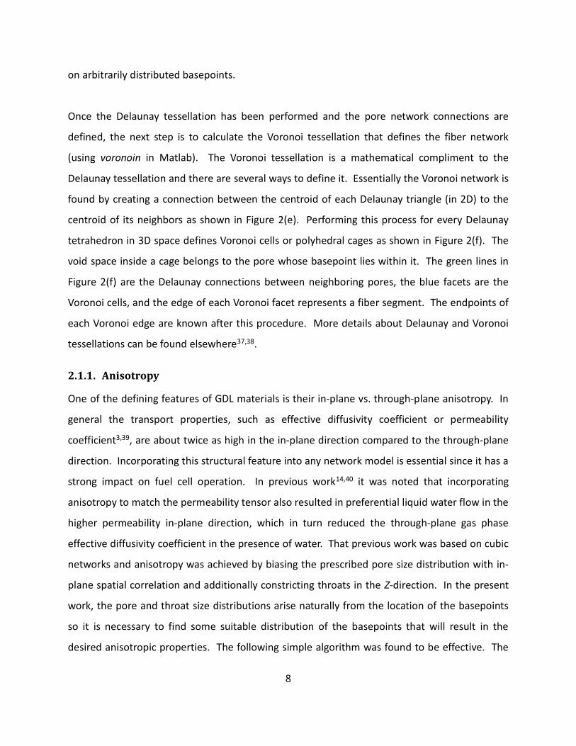
on arbitrarily distributed basepoints.

Once the Delaunay tessellation has been performed and the pore network connections are

defined, the next step is to calculate the Voronoi tessellation that defines the fiber network

(using voronoin in Matlab). The Voronoi tessellation is a mathematical compliment to the

Delaunay tessellation and there are several ways to define it. Essentially the Voronoi network is

found by creating a connection between the centroid of each Delaunay triangle (in 2D) to the

centroid of its neighbors as shown in Figure 2(e). Performing this process for every Delaunay

tetrahedron in 3D space defines Voronoi cells or polyhedral cages as shown in Figure 2(f). The

void space inside a cage belongs to the pore whose basepoint lies within it. The green lines in

Figure 2(f) are the Delaunay connections between neighboring pores, the blue facets are the

Voronoi cells, and the edge of each Voronoi facet represents a fiber segment. The endpoints of

each Voronoi edge are known after this procedure. More details about Delaunay and Voronoi

tessellations can be found elsewhere37,38.

2.1.1. Anisotropy

One of the defining features of GDL materials is their in-plane vs. through-plane anisotropy. In

general the transport properties, such as effective diffusivity coefficient or permeability

coefficient3,39, are about twice as high in the in-plane direction compared to the through-plane

direction. Incorporating this structural feature into any network model is essential since it has a

strong impact on fuel cell operation. In previous work14,40 it was noted that incorporating

anisotropy to match the permeability tensor also resulted in preferential liquid water flow in the

higher permeability in-plane direction, which in turn reduced the through-plane gas phase

effective diffusivity coefficient in the presence of water. That previous work was based on cubic

networks and anisotropy was achieved by biasing the prescribed pore size distribution with in-

plane spatial correlation and additionally constricting throats in the Z-direction. In the present

work, the pore and throat size distributions arise naturally from the location of the basepoints

so it is necessary to find some suitable distribution of the basepoints that will result in the

desired anisotropic properties. The following simple algorithm was found to be effective. The

9

final domain size used in this work was [LX, LY, LZ] = [750, 750, 250] where X and Y are the in-

plane directions and Z is the through-plane direction (see Figure 1). The basepoints are

distributed at random within these bounds, but prior to performing the Delaunay tessellation

they are scaled by an amount [AX, AY, AZ] = [1, 1, 2], so the points are distributed throughout an

expanded domain of [LX ·AX, LY ·AY, LZ ·AZ] = [750, 750, 500]. The values AX, AY and AZ are

referred to as the anisotropy scale factors. The resulting tessellation of these points gives an

isotropic structure, but rescaling all the coordinates back to the original domain size results in

Voronoi polyhedron’s that are flattened, which is analogous to fibers being preferentially

oriented in the in-plane direction as in real materials. Figure 3(a-c) shows the X-, Y- and Z-

components of lines connecting pore centers to throat centers, normalized by the total length

of the line. The anisotropic nature of the network can be seen in the diminished Z-components,

meaning that pore-to-throat connections tend to point in the XY direction. In an isotropic

structure, the distributions in Figure 3(a-c) would resemble random distributions. As will be

shown in the Model Validation and Results section, values of [AX, AY, AZ] = [1, 1, 2] produced the

desired anisotropic transport behavior. Distributing the basepoints in a more complex way may

be possible35, but the simple algorithm just described was sufficient for the present purposes.

2.1.2. Surface Pores

One issue with generating the Voronoi network is that many of the cells on the outer surface

are malformed. They can have vertices at infinity or they form open, incomplete tetrahedrons.

One way to solve this is to produce a Voronoi network that extends well beyond the desired

domain and then delete cells that lie outside, which will also drop the malformed cells. This

approach leads to a domain that has a “rough surface” as shown in Figure 4(a) for a 2D network.

These rough faces may be more realistic in some sense, but they pose several difficulties. They

mean that the domain length is not precisely defined, which is particularly significant in the Z-

direction since the fibrous mats modeled here a very thin. Furthermore, it is not clear how to

apply periodic boundary conditions on the edges of the domain (XZ and YZ faces) since there is

no correspondence between these faces. Finally, rough surfaces complicate transport

simulations since there is no definitive control surface through which to calculate the flux.

10

These problems can be remedied by creating flat outer surfaces, which was accomplished here

in the following simple manner. When a set of basepoints is mirrored about a line (in 2D) or

plane (in 3D) of reflection, the Voronoi tessellation will contain a set of cells with edges lying on

the axis of reflection. Since the axis of reflection is a straight line, this means that the edges of

the Voronoi cells will form a straight line as well. The result of this approach is shown in Figure

4(b) for a 2D domain. Similar results are achieved in 3D by mirroring the domain in all 6

directions, as shown in Figure 1.

One of the drawbacks of mirroring the domain to create flat surfaces is that the surface pores

and throats tend to be larger than the average size, which is dominated by the more numerous

interior cells. This may actually be desired on the Z faces, which represent the surface of the

fibrous mat where larger surface pores might be expected since pores are bounded by open

space rather than more fibers and hence are more open. For the edges of the domain (X and Y

faces) however, this is not desirable since these edges should be representative of the interior

points. To create smaller pores along these edges it is possible to seed the basepoints with a

slightly higher local density so Voronoi cells end up more closely packed in these regions. To

accomplish this, basepoint coordinates (X, Y, Z) are generated randomly then discarded or kept

based on a probability that is a function of their position. The probability of a point being

rejected is 0 at the edges of the domain, and increases away from the edges. This can be

described as follows:

Random

a

nb

bm

1 (1)

where nRandom is a random number between 0 and 1, m is the normalized m-position of the

point (where m can be either x, y or z), and a and b are adjustable parameters that control how

quickly and by how much the likelihood of keeping a point decreases away from the boundary

of the domain. Points are generated and subjected to this selection scheme until the desired

number of final points has been added. In the present model values of a = 35 and b = 0.2 were

used, and m was either X or Y. The point density near the Z-faces was not increased, which has

the effect of creating larger pores on these faces in accordance with X-ray tomography data of

11

porosity profiles41,42. The number of basepoints per unit volume controls porosity of the

network, as described in the next section. This procedure could also be used to impart porosity

profiles into the network by creating internal regions of high and low basepoint density but this

was not explored in the present work.

2.2. Porosity

The porosity of the network is calculated by generating an image of the fibers defined by the

Voronoi edges. This is accomplished by first creating a blank 3D image equal to the domain size,

then drawing a single pixel-width line segment for each edge of the Voronoi tessellation. Since

the endpoints of each Voronoi edge are known, it is straightforward to connect them using the

Bresenham line algorithm. Once all the Voronoi edges are added to the image, a distance

transform of the pore space is performed. The resolution of the image is 1 m3 per voxel, so

voxels within fD/2 of the Voronoi edge voxels are set to solid to represent the thickness of the

fibers, where fD is fiber diameter. The resulting 3D image of the fiber structure is shown in

Figure 5(a) and 2D cross-sections of the solid image in the through-plane and in-plane direction

are shown in Figure 5(b). Porosity is determined from this image by counting the number of

void voxels in each XY slice and determining a porosity profile as shown in Figure 5(c). Note that

the flat surfaces of this network lead to many fibers aligned with the outer faces so the porosity

there is unrealistically low, rather than approaching 1.0 as expected in reality41,42, but it

transitions quickly to a stable value that represents the internal structure. The median value of

this porosity profile is a good representation of the internal porosity and this is used to

determine the bulk porosity of the model. The number of basepoints is chosen such that the

desired porosity is achieved using a fixed value for fD of 10 m which can be determined from

SEM images of GDL materials. About 18,000 pores per mm3 resulted in a valid porosity

between 0.75 and 0.77, which corresponds to 2500 pores in the domain size simulated here

(750 ×750 × 250 µm).

2.3. Pore and Throat Sizes

In conventional pore network modeling, pore and throat size distributions are prescribed14. This

12

is generally done on a trial-and-error basis while attempting to match porosimetry and absolute

permeability data simultaneously. One of the most useful features of the present modeling

approach is that pore body and throat size are fully defined by the Voronoi polyhedrons so they

arise from the physical construction of the fiber network itself. Once the density of basepoints

is found that gives the desired porosity (for a given fiber diameter), then all of the other

structural features of the network are determined. Each pore body in the network is defined by

a Voronoi polyhedron as shown in Figure 2(f). These polyhedrons have a definite size

determined by the proximity and density of neighboring pores. The pore volume (as well as

pore radius, aspect ratio, etc.) arises directly from the shape of its Voronoi cell. Additionally, the

set of Voronoi cells fill space completely, so each facet of a Voronoi cell is shared with a

neighboring cell. Transport of any quantity (liquid water percolation, gas diffusion) between

neighboring pores must occur through these facets, which therefore represent throats. Since

the size of each Voronoi cell is fixed during the tessellation stage, the size of each facet is also

known. To complete the analogy between Voronoi edges and fiber segments a fiber diameter

must be assigned. This allows the extraction of throat sizes and pore volumes in the presence

of the solid material. Adding a thickness to the Voronoi edges means that a portion of each

facet will be occluded, so the amount that remains open defines the size of the pore throat.

Figure 6(a) shows a single throat facet with the fiber diameter occluding part of the opening.

Figure 6(b) shows a small section of the Voronoi tessellation expanded to the thickness of a

fiber diameter. The extraction of these geometrical properties is described below.

It is possible to calculate the area or dimensions of a Voronoi facet just from knowledge of

vertex coordinates (which are known after the Voronoi tessellation algorithm), but

incorporating the impact of fiber diameter on throat dimensions is more complicated. For

instance, adjusting the points by applying an inward offset of the vertices by fD/2 is not

sufficient since the polygon can become self-intersecting. To avoid this problem, image analysis

techniques are used. Each facet to be analyzed is a 2D polygon that is positioned in 3D space.

To generate a useful image that can be analyzed for size and other shape factors, the facets

must be rotated to lie flat in a 2D plane. The facet is rotated by first finding the unit normal to

13

the throat facet, u

. Next the axis of rotation is found that will orient the unit normal in the

positive Z-direction, AXISn

= u

[0 0 1] = [a b c]. The necessary angle of rotation about this axis

can be found from trigonometry as = cos-1(c). A rotation matrix M is constructed using the

components of AXISn

and the angle of rotation as follows:

coscos1sincos1sincos1

sincos1coscos1sincos1

sincos1sincos1coscos1

2

2

2

cabcbac

abcbcab

baccaba

M (2)

Finally, the rotation is applied by multiplying the [X, Y, Z] coordinates of each corner of the facet

by M. The rotated points are inserted into an empty image as single pixels, and the facet is

filled to create a solid polygon for suitable for image analysis (using Matlab's regionprops tool).

Once the filled facet image is generated, it is eroded from all sides by fD/2 to account for the

occlusion by the fibers (using Matlab's imerode tool). The resulting polygon can then be

subjected to any number of image analysis techniques to extract size information, such as area,

maximum inscribed circle, equivalent diameter and if the throat is skewed, eccentricity and

equivalent ellipse dimensions (all offered by Matlab's regionprops). The procedure is repeated

for every facet of every Voronoi cage in the network, which is time consuming, but only needs

to be performed once for a given network realization (The entire network generation and size

extraction requires about 30 minutes on a decent desktop workstation with 8 cores and 12 Gb

of RAM). The resulting distribution of throat sizes is given in Figure 7(b) where the reported

diameter is that of a circle with an equivalent area. The distribution has a log-normal shape

with a mean value around 20 m, which is close agreement with the sizes used in previous work

with cubic networks14. Recall that in cubic networks the throat size distribution is determined

by a trial and error procedure until the simulated capillary pressure curve matches mercury

intrusion porosimetry (MIP) data. The fact that a similar size distribution arises naturally from

this Voronoi tessellation procedure is encouraging. A significant number of throats are fully

occluded by the fiber, and these are not included in this distribution (rather than reporting their

diameter as 0). Figure 7(d) shows the connectivity distribution of the network with fully

occluded throats removed. This distribution is in excellent agreement with the ‘topologically

14

equivalent’ network of Luo et al28 who report an average coordination number of 13 with a

minimum of 2 and a maximum of 51 for Toray materials.

Pore volumes must also be calculated with consideration for the volume displaced by the fibers,

and this is also accomplished using image analysis. An empty 3D image equal in size to the

specified domain is first generated. Next, every voxel in the image is tested to determine which

Voronoi cell it belongs to, and is assigned a label corresponding to its owner. The test for

determining if a voxel is within a Voronoi cell is performed using inhull43. To save computation

time only voxels within the bounding box of Voronoi cell i are tested for membership within cell

i. The resultant label image is multiplied by the inverse fiber image (with void set to 1 and fiber

set to 0) and the volume of a given cell is found by summing the number of voxels containing its

corresponding label number. Figure 7(a) shows the pore size distribution reported as the

diameter of a sphere with an equivalent volume.

2.4. Throat Length

Fibrous materials such as GDLs are a challenge to model using pore networks. Their open

structure and high porosity make it difficult to determine where one pore ends and the next

begins. Throats in these materials are only constrictions between fibers, and bear no

resemblance to the capillary tubes that are typically considered in conventional porous

materials such as rocks and stone. In these Voronoi networks, the location of a throat is

precisely defined by the facets of the Voronoi tetrahedrons; however, it is not as clear how long

a throat should be or whether throat length is even a meaningful or useful parameter.

Thompson35 specified throat length as the fiber diameter, which is naturally the length of the

constriction between neighboring pore bodies. In his work, Thompson35 focused on calculation

of permeability which is highly sensitive the size and length of constrictions so he had to make

numerous assertions about the impact of throat size, length, shape, converging-diverging

geometry, etc. In the present work, which aims at determining effective diffusivity rather than

permeability, the transport distance between two pores is found from the total pore-to-pore

length, without consideration for the pore body and throat lengths. The area of the throat

15

(Voronoi facet) is considered to apply to the entire length of the conduit.

The first step to getting realistic values for throat length is to relocate the basepoints to the

actual centroid or center-of-mass of each Voronoi cell. Without this readjustment, the

basepoint for a given cell could lie almost anywhere within the cell. Shifting the basepoint to

the centroid ensures that the cumulative distance from the cell basepoint to each of the throat

centers is minimized. Similarly, throat centers are also defined as the centroid of the facet.

Centroids of convex polygons in 2D and 3D can be found using the centroid function44. The

basepoints and throat centers in Figure 4 have been adjusted in this manner. Once the pore and

throat centers are moved it is possible to define the distance between pore centers as the sum

of the lengths of straight lines connecting two pore centers to the center of their common facet

as depicted in Figure 4. This procedure means that the network no longer strictly adheres to

the definitions of the Voronoi and Delaunay tessellations, but the geometry is still fully defined

and suitable for the present purposes. Figure 7(c) shows the distribution of the pore center to

pore center lengths, with the mean value around 50 m, which is somewhat larger than the

lattice spacing value of 25 m used in previous pore network modeling studies14 of Toray 090

using cubic networks. The increased value found here is an indication that the present model

successfully reduces the constraints encountered with the cubic model, namely that the lattice

spacing was kept small to achieve high porosity which had the undesirable side-effect of limiting

the maximum pore size to the lattice spacing. The reported pore-to-pore spacing value of 50

m is an average, independent of direction. Due to the anisotropy added to the network the

throat lengths and pore-to-pore spacing in the Z-direction will be less than the X and Y

directions. Figure 3(d-f) show the pore center-to-throat-center length distributions for the

network as given by the X-, Y- and Z-components of the line (vector) connecting each pore

center to its neighboring throat centers. Clearly, the lengths of the pore-to-throat connections

in the Z-direction are shorter than the X and Y directions by about half meaning that the pore-

to-pore center spacing in the Z-direction will be smaller than the average value of 50 m.

Similarly, the pore-to-pore spacing in the X and Y directions will be even larger, which is actually

in better agreement with SEM images of GDLs. Note that the values in Figure 3(d-f) are pore-to-

16

throat lengths, while the values in Figure 7(c) are pore-to-pore lengths. The latter value is

comprised of 2 pore-to-throat connections and there is a low probability of both being short,

resulting in a more Gaussian distribution.

2.5. Diffusive Conductivity

The diffusive conductivity between two neighboring pores i and j is defined as:

ij

ijABijD L

AcDg , (3)

where c is the molecular density of the gas, DAB is the open-space diffusion coefficient, A is the

area of the conduit or throat connecting pores i and j, and L is the length of the conduit

connecting pores i and j. The determination of the total conduit length, Lij, was discussed above.

The area, Aij, of the conduit is taken as the area of the throat connecting the two pores. As

throats are smaller than pores by definition, the use of the throat area to represent the entire

conduit may appear overly conservative. It must be remembered, however, that many throats

are connected to the same pore center, so using larger areas more representative of the pore

size would effectively lead to the same pore volume contributing to the conductivity of multiple

conduits. The conductivity given by Eq.(3) is used in Fick’s law to calculate the diffusive

transport of species A between pores i and j:

jAiAijDijA xxgn ,,,, (4)

where nA is the molar flow rate between pores i and j, and xA is the mole fraction of species A in

each pore. The total effective diffusivity of the network is found by calculating the total molar

flow through the inlet surface, and using Fick’s law over the entire domain:

OUTAINA

EFFA xx

L

cADn ,, (5)

where L is the length of the domain, xA,IN and xA,OUT are the gas phase concentration of species A

specified in the Dirichlet boundary conditions.

2.6. Capillary Pressure

The throat openings resulting from this network generation approach are multisided polygons

and arbitrary shape. The geometry of each facet is known exactly, but it is challenging to relate

17

this information to the capillary pressure required for invasion. It is customary to use the so-

called Washburn equation to relate these parameters45:

iiC r

P cos

2, (6)

where PC,i is the capillary pressure (PL – PG) that must be applied to the invading fluid to

penetrate throat i, ri is the radius of throat i, is the contact angle measured through the

invading liquid, and is the surface tension of the gas-liquid interface. The Washburn equation

was derived assuming straight, cylindrical pores. This equation does not adequately describe

the invasion of water into GDL-type materials46. Experimental data consistently show46 that

positive values of PC must be applied to inject water into non-wetproofed GDLs which

presumably have contact angles below 90°. Since the throats are multisided polygons with

arbitrary aspect ratio it is not a simple matter to define ri, let alone determine the

corresponding breakthrough pressure47. Common options include using Eq.(6) with the radius

of the maximal inscribed circle and the radius of a circle with equal area. The impact of these

different definitions is explored in the Model Validation and Results section below.

In addition to their size, another important feature of the throats is their converging-diverging

nature resulting from the fibrous solid structure. Mason and Morrow48 discuss the impact of

such geometry on capillary breakthrough pressures, and present the Purcell toroid model as a

means of accounting for this geometry. This model leads to the following analytical expression

that can be used as a direct substitute for the Washburn equation (Eq.(6)):

cos121

cos2,

i

DiiC

rfr

P (7)

where is the contact angle measured through the invading phase, ri is the half-spacing

between the fibers and fD is the fiber diameter. fD is assumed be constant which is valid for GDL

materials. is the angle beyond apex of the curved throat (i.e. the smallest constriction) where

the maximum meniscus curvature occurs:

18

D

if

r21

sinarcsin

(8)

The angle is defined such that it is 0 at the constriction of the toroid and a negative value for

menisci that push through the opening as is the case for the invasion of water into a dry GDL.

When displacing a perfectly wetting fluid the angle is 0 and Eq.(7) reduces to the Washburn

equation. As the system becomes more neutrally wettable, the effects of the diverging

geometry become more significant. Using Eq.(7) also means that invading fluids with a contact

angle below 90° will still require positive capillary pressures for invasion, in agreement with

experimental observation46,49-52. Eq.(7) also (at least qualitatively) explains the hysteresis

observed in the same experiments, where negative pressures are required to withdrawal water

despite positive pressure for injection; an explanation forwarded by Harkness et al51 and also

discussed by Mason and Morrow48. Water withdrawal (or air imbibition) is not considered in

this work since imbibition is a significantly more complex process requiring consideration of

cooperative pore filling, snap-off, trapping and so on.

One added benefit of the Voronoi network generation approach is that 3D images of the fiber

structure can be generated. It is possible to perform direct numerical simulations on such

images. In the present work, drainage capillary pressure curves are calculated using a variation

of the image-based morphological image opening (MIO) algorithm outlined by Hilpert and

Miller53. This method has been applied to GDL systems by Schulze et al54. Instead of using

dilation and erosion, however, the distance transforms were utilized as follows. A distance

transform for the entire pore space is computed (using bwdist in Matlab). All voxels located a

distance Ri or farther from solid are set to 1 (and the remainder set to 0) to create a set of ‘seed

points’. Any seed points that are not connected to the invasion faces are removed. This is

accomplished by performing a cluster labeling routine (using bwlabeln in Matlab), identifying

the invading clusters as those present on the invasion face(s), and setting all non-connected

seed points to back to 0. A second distance transform is then computed relative to the surviving

seed points, and all voxels within Ri are set to 1 (and the remainder set to 0). By combining the

19

seed points from the first step with the voxels found in the last step, the invading water

configuration is obtained. Repeating this procedure for decreasing sizes of Ri yields a capillary

pressure curve (using the Washburn equation to relate Ri to PC and counting the fraction of

filled vs. unfilled voxels to determine SW). Typical images resulting from the MIO simulation are

shown in Figure 8. Figure 8(a and b) show two invasion pressures in a small domain with the

fibers removed to reveal the water. Figure 8(c) shows a full domain of the sized used for the

pore network model simulations. The fibers are drawn semi-transparently.

There are two key limitations to the MIO algorithm. Firstly, coalescence of menisci is not

accounted for. That is, if the tips of two invading fingers touch each other, they would

realistically be expected to coalesce but this does not occur in such a calculation. Second, and

more importantly, the invading water curvature is limited to spherical caps, while in reality

water configurations can be ellipsoidal or even more complex shapes depending on the solid

geometry. The result is that MIO invasion pressures will be overestimated. Nonetheless, these

simulations still provide a useful comparison to the network model, since menisci coalescence is

also neglected (at least in the present work) and throat breakthrough pressures can be

computed from inscribed circles, which corresponds to spherical caps. Agreement between

these two calculations can therefore confirm that throat sizes and connectivity are being

correctly described in the pore network approach.

2.6.1. Late Pore Filling

The heuristic, rule based invasion algorithms used by pore network models to efficiently track

water movements and configurations means that a pore is deemed either filled or not filled.

This method does not explicitly resolve structural features smaller than the scale of a single

pore or throat, such as surface roughness, corner, crevices, or cracks. Deeming a pore

completely filled upon invasion is unrealistic since the sub-pore scale features can represent a

noticeable volume, which is slowly filled as capillary pressure is increased, a phenomena termed

“late pore filling”. Late pore filling can be added to pore network models in a relatively simple

manner. Upon invasion, a pore is deemed to be only partially filled to some fraction S’WP of its

20

total volume. As pressure is increased above the initial entry pressure PC,i of a given pore i, the

remaining wetting phase in that pore is slowly reduced with each subsequent increase in

pressure according to:

C

iCWPiWP P

PSS ,

, (9)

where is a fitting parameter that controls how rapidly the residual wetting phase is drained

with increasing pressure. Eq.(9) is calculated for each pore (if PC > P’C,i), and the actual volume

of invading fluid in each pore is found from (1 – SWP,i)·VP,i where VP,i is the volume of pore i. It

was found in the present work that S’WP = 0.25 and = 1 were suitable for matching

experimental data. These values are very close to those used in previous work based on regular

lattices with cubic pores14. Values of S’WP could be determined for each individual pore based

on their unique geometry, but this was not done here.

2.7. Percolation Algorithms

The multiphase transport scenarios explored in this work require two sorts of invasion

algorithms as has been previously discussed40. Access limited ordinary percolation (ALOP) is

used to simulate capillary pressure experiments where a fixed pressure is applied to a sample

and the amount of non-wetting fluid injected at each pressure is monitored. This is simulated

by first identifying all the throats in the network that can potentially be invaded at the specified

pressure. Any throats identified as invaded but are not connected to the injection face, either

directly or through a pathway of invaded pores and throats, are set back to a ‘not invaded’ state.

This ensures that only pores and throats that are physically accessible from the injection source

are invaded. The injection source can be one or more, full or partial faces, or even internal

pores if the application warrants. For computational efficiency purposes, the actual execution

of this calculation is done in terms of clusters of connected pores rather than on a pore-by-pore

basis. In conventional cubic networks the Hoshen-Kopelman algorithm55 is used, but in random

networks a more general algorithm is required. Union-find algorithms, and in particular the

weighted quick union with path compression algorithm (WQUPC), are the most efficient known

methods for this task56. WQUPC was adapted in the present work, using an adjacency matrix

21

representation of the network57. An adjacency matrix is a sparse N-by-N matrix, where N is the

number of pores in the network. The connection between pores i and j are noted by placing a 1

at location (i,j) in the adjacency matrix. The benefit of using an adjacency matrix is that any

network architecture (random, cubic) and any dimensionality (2D, 3D) can be represented with

equal ease. To perform the ALOP simulation, the nonzero entries in the adjacency matrix are

replaced by the calculated breakthrough pressure of the throat connecting two pores. All

throats with a breakthrough pressure greater than the applied pressure are set to 0 (i.e. their

connection is removed from adjacency matrix). The WQUPC algorithm then finds connections

between invaded throats in the adjacency matrix and returns a list containing the cluster

number of each invaded pore.

Invasion percolation (IP)58 is used to simulate constant rate injection into a sample where fluid

flows into the material in a pore-by-pore fashion following the path of least resistance (i.e. via

the throat with the lowest breakthrough capillary pressure that is currently accessible by the

invading fluid). As discussed previously40 IP is necessary to capture the breakthrough conditions

(pressure and saturation) of thin materials to match experimental data. IP is simulated by

generating a list of accessible throats that are connected to the injection source(s), then

invading that with the lowest entry pressure, resulting in the filling of a single pore connected to

the invaded throat. The throats connected to the newly invaded pore are added to the list of

accessible throats, and so on. Unlike the ALOP algorithm, the IP simulation must be done on a

pore-by-pore basis and can therefore be time consuming on large networks. It has been

noted59 that IP is related to the minimal weighted spanning tree commonly considered in graph

theory. Glantz and Hilpert60 present a detailed algorithm for computing various IP processes

starting with the minimal spanning tree. In the present work, only drainage without trapping

was considered, so a custom algorithm was developed based on Prim’s algorithm for finding the

minimal spanning tree. The present method was modified to stop when one or more specified

outlet sites are invaded, and to allow for loops in the tree, which occur when a throat

connecting two invaded pores is invaded.

22

2.8. Materials Modeled

The parameters for the present work are chosen to produce a model of Toray 090 or 060, for

which numerous sources of experimental data are available. The thickness of Toray 060 and 090

were measured using a Mitutoyu digital caliper (1 m resolution) as 220 and 275 m

respectively. The porosity of these two materials is widely reported as 78% prior to treatment

with PTFE, and 76% for 10% PTFE by weight. The fiber diameter can be easily found from SEM

images to be 9-10 m. Fluckiger et al39 reported extensive data on the effective diffusivity

tensor of Toray 060 and these will be used for comparison. Capillary pressure data for water

and mercury intrusion have been measured for treated and untreated Toray 09052,61.

23

3. Model Validation and Results

3.1. Capillary Pressure Curves

3.1.1. Mercury Intrusion Porosimetry

Figure 9 compares capillary pressure curves obtained using various modeling approaches to

experimental mercury intrusion porosimetry (MIP) data52 for Toray 090 with 10% PTFE loading

by weight. The MIP data were obtained on a single piece of GDL (10 mm by 30 mm), rather

than a stack or bundle as is often done to maximize invaded volume and increase resolution.

The main impact of performing MIP on a single piece of GDL is that the pore volume accessible

at low pressures is a significant fraction of the total volume. This behavior is often described as

the “finite size effect”, and is a combination of several mechanisms. Firstly, from the view of

percolation theory, the volume of invaded sites is 0 on infinite networks prior to the percolation

threshold. On finite sized networks, however, the non-negligible volume of invading fingers is

manifested as an S-shape capillary pressure curve rather than a sharp transition from SNWP = 0

to SNWP > 0. Secondly, the surface pores tend to be somewhat larger than internal pores due to

the construction of the material, as shown by porosity profile measurements of GDLs41,42. In

thin materials, these pores will represent a significant fraction of the population, resulting in a

bimodal pore size distribution with a small hump in the low-pressure region. A third factor is

that surfaces have a large-scale roughness that appears as easily invaded pore volume filled at

low pressures. All of these effects are only detectable on small samples and therefore each

contributes to general observation of finite size effects. In thin materials like GDLs such effects

are an integral part of their capillary behavior, so efforts are made to include this behavior in the

present model.

All simulations (both ALOP on the pore network and MIO on the Voronoi fiber image) were

performed on a domain equivalent to a single layer (250 m), though the sample size was

limited to 0.75 mm by 0.75 mm due to computational resources. The non-wetting fluid in all

simulations was able to invade from all faces and edges, to maintain the analogy to MIP where

24

mercury fully surrounds the sample prior to invasion. Finally, to relate the present simulations

to MIP data it is necessary to convert the model results, which are all based on sizes, to capillary

pressure. This was done using Eq.(6) with a mercury surface tension of 0.46 N/m and a

contact angle of 140°.

The MIO based curve shows significantly higher capillary pressures than the experimental data.

This is because in MIO the breakthrough of a throat or constriction only occurs when the

invading fluid curvature is reduced to the radius of an inscribed circle (as discussed in Section

2.6). In reality, the breakthrough pressure will be lower since the complex geometry (e.g.

aspect ratio greater than unity) will result in a smaller mean radius of curvature. This

explanation is confirmed by the good correspondence between the MIO curves and the pore

network model when throat sizes are described by the radius of an inscribed circle. This match

also confirms that the image analysis routines (outlined in Section 2.3) successfully extracted

throat sizes. It was found that using the equivalent diameter as the characteristic throat radius

in Eq.(6) provided an acceptable match between the pore network model and the MIP data.

The equivalent diameter gives a larger estimate for throat size that successfully accounts for the

smaller meniscus curvature in throats that are not symmetrical. The good match between the

MIP data and the pore network model indicates that the pore and throat size distributions in

the Voronoi network are a good approximation of the real fibrous GDL material. As mentioned

in the Introduction, one of the motivations for developing this random network architecture

was that the previous cubic network models produced capillary pressure curves that were much

steeper than experimental data due to an overly constrained pore size distribution. It can be

seen in Figure 9 that the random network architecture has successfully remedied this problem.

The deviation in the high saturation region can be attributed to late pore filling effects. The

solid lines in Figure 9 show the results of the pore network model without considering late pore

filling (i.e. a pore is deemed completely filled as soon as it is invaded). When the late pore filling

correction (Eq.(9)) is included, the pore network model based on inscribed circles matches the

MIO curve almost exactly (dashed lines). The MIO simulation automatically includes late pore

25

filling effects to some extent since the fluid slowly inflates to conform to the solid shape as the

pressure is increased. The late pore filling behavior of the MIO curve is in qualitative agreement

with the MIP data, though the effect is more pronounced in the experimental data. This can be

attributed to the fact that details of fiber surface roughness were not resolved in the generated

image on which the MIO simulation was performed. The late pore filling curve with equivalent

diameter throats matches the experimental data fairly well. A perfect match could be obtained

by increasing the S’WP value in Eq.(9), but this would not necessarily be meaningful since it may

be the case that the network simply needs more small pores.

Finite size effects are also present in all modeled data because of the thin domain, and they all

agree fairly well with the MIP data. Because of the artificially flat surfaces included in the

model, the impact of large-scale roughness is not present. The MIO curve follows the MIP data

quite closely at the lowest capillary pressures. This indicates that surface roughness is not a

factor in the MIP data, which is expected since the sample is surrounded by mercury. In the

MIO simulation, fluid fingers can partially inflate into a pore without actually breaching the

throat, which leads to the slightly larger finite size effects in the MIO simulation than the ALOP

curves.

3.1.2. Water Injection

Experimental capillary pressure data for water injection are shown in Figure 10 along with

various simulated curves. The water injection data was obtained for Toray 090 with 10% PTFE

by weight. The experiments were conducted on a single circular sample of 19 mm diameter52.

Finite size effects are very prominent in this data. The breakthrough or percolation point in

these materials was measured previously and found to be approximately located at the start of

the sharp rise at SW 0.25, so the volume injected prior this point is due to the various finite

size effects mentioned above. The initial jump from SW = 0 to 0.1 is likely due to the filling of

large-scale surface roughness, or even gaps between the sample and the hydrophilic membrane

below the sample. The absence of this jump in the MIP data is likely because the sample is

surrounded by mercury so no such gaps are present prior to injection. The slow increase from

26

SW = 0.1 to 0.3 is probably a combination of larger surface pores and non-percolating fingers of

invading fluid. With the exception of the dashed line (to be discussed below), the simulation

results in Figure 10 all use Eq.(6) with a water-air surface tension = 0.072 N/m and a contact

angle = 105° to relate size to pressure. The choice of = 105 is somewhat arbitrary, but was

considered to be a fair average between carbon fibers ( 80) and PTFE ( 112). The nature

of the experimental setup used to collect the data means that water was invaded from only one

face, so all of the simulation results were obtained with injection into the Z = 0 face in order to

correspond better with the experiment.

The simulations were conducted on the same 250 × 750 × 750 m domain as the MIP

simulations. All the ALOP simulations include the late pore filling model with the same

parameters as for the MIP case, and this seems to capture the effect quite well. As expected

the MIO and ALOP with inscribed circle match each other quite closely and the ALOP with

equivalent diameter shows lower pressures. The most striking feature of the results shown in

Figure 10 is that all the models (with the exception of the dashed line, to be discussed below)

show much lower capillary pressures than the data, which is opposite the trend seen in the MIP

case. In order to match the experimental data, a value near 130 would be required but this is

much higher than the contact angles of any of the constituent materials.

The MIP simulations confirmed that the throat sizes in the model were a good approximation,

so this discrepancy must be due to some other factor. It’s possible that small-scale surface

roughness of the fibers leads to an increased effective contact angle by the Wenzel or Cassie-

Baxter effects62, but this was not apparent in the MIP data where the traditional contact angle

of 140° was acceptable, so was ruled out here. A more likely explanation for this paradoxical

behavior is that Eq.(6) is not a valid means of relating throat size and invasion pressure in

neutrally wettable systems. Eq.(6) was derived for straight, cylindrical tubes, whereas the

throats in the present material are defined by fibers. The converging-diverging nature of the

constriction between two fibers can have a very large effect on the capillary breakthrough

pressure. When the curved geometry of the pore throats is accounted for with Eq.(7), in

27

conjunction with the equivalent diameter, the agreement between the data and the ALOP

model is remarkably close as can be seen from the dashed line in Figure 10. The amount by

which the throat breakthrough pressure increases depends on the fiber diameter, fiber spacing

and contact angle. This effect is most pronounced at contact angles near 90°, which is why this

behavior is so prominent in water invasion simulations, while the MIP results agreed quite well

without this consideration. This strongly suggests that Eq.(7) be used to relate throat size to

pressure when modeling multiphase flow in fuel cell electrodes and GDL. This finding casts

considerable doubt on the common belief that MIP provides pure pore size information, and all

other fluids can be modeled by adjusting for changing surface tension and contact angle. This

concept has been taken so far as to use a contact angle distribution as a fitting parameter63,64 to

rectify the differences between mercury and water injection data. Clearly, the explanation

offered by the converging-diverging throat model is much more feasible. It is also easier to

implement since Eq.(7) is an explicit analytical expression and can be used in any situation or

calculation where the Washburn equation is normally applied without any increased

computation. The only additional information required for its use is the fiber diameter, which is

straightforward to measure, especially in GDLs where fiber diameters are monodisperse.

The late pore filling model provides an excellent match to the experimental data in the high-

pressure region. The finite size effects in the low-pressure region do not appear to be well

described by the models. If the jump from SW = 0 to SW = 0.15 were not present, the agreement

in this region would be much better. As mentioned above, the experimental setup used to

collect the water-air data is susceptible to gaps below the sample that could cause the observed

jump. Capillary pressure curves on compressed samples do not show this jump, indicating that

such gaps are eliminated when the GDL contacts the hydrophilic membrane more tightly.

3.1.3. Water Breakthrough Conditions

Using the invasion percolation (IP) algorithm rather than ALOP it’s possible to determine the

specific water invasion configuration required to achieve breakthrough. As depicted in Figure

11(a and b), liquid water invades from the entire Z = 0 face and the simulation is stopped when

28

water breaches sample at the Z = 250 m face at a single point. The simulation predicts a

breakthrough saturation of 0.20 which is in good agreement with previously reported

experimental measurements40. This saturation value does not include late pore filling effects,

since it is not obvious which capillary pressure to apply in Eq.(9) given that the pressure applied

during invasion percolation varies with time as different size throats are invaded65. In any case,

the late pore filling effect would reduce this value by at most 25% so it still agrees well with the

experimental values which range between 0.15 – 0.20. The saturation profile resulting from the

IP process is shown in Figure 11(c). This is in agreement with other PNM predictions17,24,28 and

X-ray tomography data42, but is at odds with the saturation profiles found in continuum models

based on unsaturated flow theory and generalized Darcy’s law for multiphase flow. One thing

that can be inferred from this saturation profile is that it would lead to very poor fuel cell

performance since most of the pores on the catalyst layer face (Z = 0) are filled with water. As

Ceballos and Prat17 have shown, reducing the number of injection sites on the invasion face

ameliorates this situation, and leads to lower overall GDL saturation. This mechanism has been

proposed as one of the ways a microporous layer improves fuel cell performance13.

3.2. Effective Diffusivity

3.2.1. Dry Diffusivity Tensor

Diffusion of gas through the pore space of the GDL is a vital parameter in fuel cell operation.

Reactive species (oxygen on the cathode) diffuse from the flow channel to the catalyst layer in

the through-plane direction (Z-direction), and reaction products (water vapor on the cathode)

counter-diffuse out of the cell. The in-plane diffusion (X- and Y-direction) of species to and from

areas under the channel ribs is also critical. In fact, the main purpose of the GDL is to act as a

spacer to allow gas and vapor diffusion to areas of the catalyst layer that would otherwise be

masked by the channel rib. The fibrous nature of GDL materials means that the in-plane and

through-plane directions have significantly different effective diffusivity coefficients. Kramer et

al66 and Fluckiger et al39 reported experimental values of DEFF in uncompressed Toray 060. They

found that normalized effective diffusivity values D’EFF (D’EFF = DEFF/DAB) varied between 0.4 - 0.5

for the in-plane direction and 0.20 - 0.25 for the through-plane direction, where DAB is the

29

diffusion coefficient in open space.

The present pore network model incorporates anisotropy into the construction of the network.

This results in the average direction of a pore-to-throat connection to be oriented in the XY

plane as shown in Figure 3. Consequently, gas diffusion in the Z-direction must follow paths

that are predominantly in the X or Y directions, which lead to more tortuous or elongated paths

resulting in an anisotropic effective diffusivity tensor. The X, Y and Z components of the

effective diffusivity in the present network are shown in Table 1 for various combinations and

amounts of anisotropy in the Y and Z directions corresponding to anisotropy scale factors [ AX,

AY, AZ ] = [ 1, 1…3, 1…3 ] . The values of [ AX, AY, AZ ] = [ 1, 1, 2 ] lead to in-plane and through-

plane effective diffusivity coefficients of 0.45 and 0.23, respectively; which matches the

experimental data of Fluckiger et al39 quite well, and these values are used for all simulations in

this work. From the other results in Table 1, it is also apparent that anisotropy can be increased

or applied in multiple directions to obtain a range of effective diffusivity tensors. This might be

useful for modeling a material such as SGL10 series which was previously found to have some

in-plane anisotropy for gas permeability measurements3. The anisotropic scale factors need not

be integer values, so a high degree of flexibility is possible.

3.2.2. Relative Effective Diffusivity

Estimation of the gas phase effective diffusivity coefficient in partially water saturated porous

materials is one of the main goals of pore network models. This parameter is very difficult to

measure experimentally. It requires creating and maintaining an appropriate and known liquid

water distribution in the sample while simultaneously measuring gas phase diffusion, which in

itself is not trivial on samples that are only 250 m thick. Most measurement of effective

diffusivity in the through-plane direction have used stacks of 10-20 samples39 or used artificially

thick samples67. Hwang and Weber68 recently reported progress in the measurement of

effective gas diffusion coefficients through partially saturated GDLs. The comparison of their

experimental data to the present model is not straightforward however, as will be discussed

below.

30

Gas phase diffusivity was simulated in both the in-plane (X or Y) and through-plane (Z)

directions as a function of invading water saturation. In all cases water was injected into the

GDL from the Z = 0 face according to the ALOP algorithm. Figure 12 shows a 3D view of the

network with each cell colored according to the concentration of the diffusing gas species with

blue cells showing the locations of invading water clusters. Repeating this calculation for both

the in-plane and through-plane direction at increasing applied pressure yields the results in

Figure 13. These data are reported as the relative effective diffusivity DrG,n =

DEFF,n(SW)/DEFF,n(SW=0) where n is the direction of the applied concentration gradient (X, Z). The

water saturation values in Figure 13 include the effect of late pore filling. Pores filled with water

were deemed to have negligible gas diffusivity even though late pore filling was applied; this

effectively assumes that the residual gas phase in an invaded pore offers no significant gas

conductivity. Both curves in Figure 13 are normalized by the effective diffusivity of the dry GDL

in the corresponding direction. As can be seen, the relative effective diffusivity in the Z-

direction decreases more quickly than in the X (and Y) direction. This is in agreement with

previous simulations14 where it was attributed to preferential flow of liquid water in the in-

plane direction since pores and throats were larger in the in-plane direction; however, since

explicit throat size assignments are made in the present model, this behavior warrants some

analysis. It is conceivable that the anisotropic network generation scheme produces some

directionally dependent throat sizes, but analysis of the throat sizes shown in Figure 14 shows

that this is not the case. Figure 14(a) shows the orientation of the throat facets in terms of the

vector components of the unit normal to each throat facet. Z-components near 1 mean that

the throat is substantially oriented in the XY plane. Figure 14(b) shows the throat size as a

function of orientation in the Z-direction, and there is very little dependence. This confirms that

throat size does not induce preferential movement of liquid in the X and Y directions. The

behavior in Figure 13 is simply the result of the invasion process, which results in a thin layer of

water-filled pores on the Z-face (a similar effect is visible in the IP water configuration in Figure

11(b)) that seriously impedes Z-direction diffusion. This effect was also present in the

previously mentioned cubic model14 but was compounded with the prescribed directionally

31

dependent throats sizes.

The Z-directional relative effectively diffusivity values here were found to decay roughly

according to (1-SW)4, while in the previous work14 a power of 5 was a closer match. The

difference can presumably be attributed to the lack of directionally dependent throats sizes.

Hwang and Weber68 found that an exponent of 3 matched their data for untreated Toray 120,

and even smaller values for treated samples. Their experimental conditions differed from the

present simulations however, so these exponents are not directly comparable. In their work,

the GDL was initially filled with water and the saturation was altered by drying, as opposed to

the present simulation where water was injected in the Z = 0 face. It is not clear what sort of

water profile would exist in the sample from such a drying procedure. The process is one of air

imbibition (i.e. water withdrawal) rather than air drainage (i.e. water injection), and it is known

from experiments on these materials52 that water becomes disconnected during withdrawal.

Furthermore, during drying air can effectively enter the sample from all faces rather than just

the injection face so the invasion configuration will be considerably different. These differences

would mean that water is much less connected, and is in the form of isolated clusters and

discrete fingers rather than filling the injection face as observed in Figure 11(b). Simulating

water withdrawal using the present pore network model remains outside the scope of this work,

so direct comparison with Hwang and Weber68 is not possible. Qualitative comparison of these

two approaches does at least suggest that relative values obtained here differ from the

experiment in the right direction and by a reasonable amount.

32

4. Conclusions

A pore network model of fibrous GDL materials was developed using a Voronoi tessellation to

represent the solid fiber structure and a Delaunay tessellation to represent the pore space. The

physical structure of a fibrous material could be mapped almost directly to the mathematical

and geometric properties of these networks. Only three adjustable input parameters were used

to construct the model. The fiber diameter, which can be easily determined from SEM images,

was used to dilate the Voronoi edges to represent fibers. This has the effect of constricting

throat sizes and reducing the total pore volume. The number of basepoints per unit volume

was adjusted until a desired porosity was achieved. The porosity, which can be determined by

MIP or gas pycnometry, was calculated from the 3D image of the Voronoi fiber network. Finally,

anisotropy was added to the network to match the experimental diffusivity tensor data39. This

was accomplished by stretching the basepoints prior to performing the tessellations, then

rescaling them back to the original position. All three of these parameters are highly

constrained. Since the fiber diameter is known, only one value of basepoint density will give

the desired porosity. Similarly, only one set of anisotropy scale factors could reproduce the

experimentally measured diffusivity tensor data. The anisotropy in the network could have

been added using different techniques, but the simple algorithm used here was sufficient.

Given the minimal fitting adjustments that were made to construct the model, its ability to

reproduce a range of GDL behavior was impressive.

The similarity of this network to a fibrous material clearly extends beyond appearance. The

physical properties of the network agreed well with previous estimates of pore size, throat size,

pore-to-pore spacing, and coordination number. The resulting pore and throat size distributions

yielded capillary pressure behavior that very closely matched mercury intrusion porosimetry

when the equivalent diameter was used in the Washburn equation. For water injection, it was

necessary to consider the converging-diverging nature of the throat constrictions in order to

match experimental data. The fact that MIP data did not require this adjustment is

understandable since this effect is more pronounced in neutral wettability systems with

33

intermediate contact angles. An analytical expression based on the Purcell toroid was used to

relate throat size (i.e. fiber spacing) to capillary pressure that incorporates this effect, while only

requiring the fiber diameter as additional information. The use of this equation over the widely

used Washburn equation is strongly recommended for modeling water injection in GDLs.

Gas phase diffusivity was also well described by this model. The anisotropy ratio was included

into the model during construction, and resulting values of the diffusivity tensor were in

excellent agreement with recent experimental results. The flat faces and edges of the network

domain were instrumental in achieving this match. In previous work, the rough surfaces made

it impossible to define a domain size to use in the calculation of the effective diffusivity

coefficient, or to define a control surface through which to determine the total flux. The flat

edges of this network arrangement can also be used to apply periodic boundary conditions,

though this was not explored in the present work. Relative effective diffusivity in partially

saturated pore networks was estimated and found to decay approximately as (1 – SW)4 in the

through-plane direction and (1 – SW)2 in the in-plane direction. This estimate is lower than

previous modeling results where an exponent of 5 found. At present no comparable

experimental data is available.

Numerous improvements and extensions can be made to this model. In this work, the Voronoi

network was only used to represent fibers and to extract information about the pore network

sizes. The Voronoi network itself could be used to simulate the electrical and thermal

conductivity of the fiber backbone. The mathematical nature of the tessellations makes it

possible to deform the networks to simulate the effect of compression on the fibrous media.

The ability to model air imbibition will be critical for generating water configurations

comparable to the recent effective diffusivity data of Hwang and Weber68. This will also be

important in any studies of phase change in the fuel cell involving evaporation. The highly

detailed information about the geometry of the network will prove invaluable. Overall, this

modeling approach shows tremendous potential for modeling the multiphase flow and

transport conditions in the atypical and non-conventional porous materials found in the fuel cell

34

electrode.

35

5. Nomenclature

Variable Name Units

An Anisotropy Scale Factor in the n Direction ---

Aij Area of Throat Connecting Pores i and j m2

Angle of Maximum Meniscus Curvature radians

c Molar Concentration mol·m-3

DAB Diffusion Coefficient m2·s-1

DEFF Effective Diffusivity Coefficient m2·s-1

D’EFF Normalized Effective Diffusivity Coefficient (DEFF/DAB) ---

DrG,n Relative Diffusivity Coefficient (DEFF,n(SW)/DEFF,n(SW=0)) ---

fD Fiber Diameter m

gD,ij Diffusive Conductivity of Conduit Connecting Pores i and j mols-1

Lij Length of Conduit between Pores i and j m

Ln Size of Domain in n-Direction m

nA,ij Molar Flow Rate Between Pores i and j mols-1

PC Capillary Pressure (PL – PG) Pa

P’C,i Capillary Pressure at which Pore i was Invaded Pa

PL Liquid Pressure Pa

PG Gas Pressure Pa

Contact Angle radians

r Throat Radius m

SW Water Saturation ---

SNWP Non-Wetting Phase Saturation ---

S’WP Residual Non-Wetting Phase ---

Surface Tension N·m-1

xA Mole Fraction of Species A in Gas ---

36

6. References

1 Weber, A. Z. & Newman, J. Modeling transport in polymer-electrolyte fuel cells. Chem. Rev. 104, 4679-4726 (2004).

2 Sinha, P. K., Mukherjee, P. P. & Wang, C. Y. Impact of GDL structure and wettability on water management in polymer electrolyte fuel cells. J. Mater. Chem. 17, 3089-3103 (2007).

3 Gostick, J. T., Fowler, M. W., Pritzker, M. D., Ioannidis, M. A. & Behra, L. M. In-Plane and through-plane gas permeability of carbon fiber electrode backing layers. J. Power Sources 162 228-238 (2006).

4 Baker, D. R., Caulk, D. A., Neyerlin, K. C. & Murphy, M. W. Measurement of Oxygen Transport Resistance in PEM Fuel Cells by Limiting Current Methods. J. Electrochem. Soc. 156, B991-B1003 (2009).

5 Hussaini, I. S. & Wang, C. Y. Measurement of relative permeability of fuel cell diffusion media. J. Power Sources 195, 3830-3840, doi:10.1016/j.jpowsour.2009.12.105 (2010).

6 Ye, X. & Wang, C. Y. Measurement of Water Transport Properties Through Membrane Electrode Assemblies. II. Cathode Diffusion Media. J. Electrochem. Soc. 154, B683-B686 (2007).

7 Gurau, V. & Mann, J. A. A critical overview of computational fluid dynamics multiphase models for proton exchange membrane fuel cells. SIAM J App Math 70, 410-454 (2009).

8 Miller, C. T. et al. Multiphase flow and transport modeling in heterogeneous porous media: Challenges and approaches. Adv. Water Res. 21, 77-120 (1998).

9 Gray, W. G. & Hassanizadeh, S. M. Paradoxes and realities in unsaturated flow theory. Water Resour. Res. 27, 1847-1854, doi:10.1029/91wr01259 (1991).

10 Rebai, M. & Prat, M. Scale effect and two-phase flow in a thin hydrophobic porous layer. Application to water transport in gas diffusion layers of proton exchange membrane fuel cells. J. Power Sources 192, 534-543 (2009).

11 Preston, J. S., Fu, R. S., Pasaogullari, U., Hussey, D. S. & Jacobson, D. L. Consideration of the Role of Micro-Porous Layer on Liquid Water Distribution in Polymer Electrolyte Fuel Cells. J. Electrochem. Soc. 158, B239-B246, doi:10.1149/1.3525626 (2011).

12 Hickner, M. A. et al. In Situ High-Resolution Neutron Radiography of Cross-Sectional Liquid Water Profiles in Proton Exchange Membrane Fuel Cells. J. Electrochem. Soc. 155, B427-B434 (2008).

13 Gostick, J. T., Ioannidis, M. A., Fowler, M. W. & Pritzker, M. D. On the role of the microporous layer in PEMFC operation. Electrochem. Commun. 11, 576-579 (2009).

14 Gostick, J. T., Ioannidis, M. A., Fowler, M. W. & Pritzker, M. D. Pore network modeling of fibrous gas diffusion layers for polymer electrolyte membrane fuel cells. J. Power Sources 173, 277-290 (2007).

15 Sinha, P. K. & Wang, C. Y. Pore-network modeling of liquid water transport in gas diffusion layer of a polymer electrolyte fuel cell. Electrochim. Acta 52, 7936-7945 (2007).

16 Hinebaugh, J., Fishman, Z. & Bazylak, A. Unstructured Pore Network Modeling with Heterogeneous PEMFC GDL Porosity Distributions. J. Electrochem. Soc. 157, B1651-

37

B1657, doi:10.1149/1.3486095 (2010). 17 Ceballos, L. & Prat, M. Invasion percolation with inlet multiple injections and the water

management problem in Proton Exchange Membrane Fuel Cells. J. Power Sources 195, 825-828 (2010).

18 Medici, E. F. & Allen, J. S. The Effects of Morphological and Wetting Properties of Porous Transport Layers on Water Movement in PEM Fuel Cells. J. Electrochem. Soc. 157, B1505-B1514, doi:10.1149/1.3474958 (2010).

19 Lee, K.-J., Nam, J. H. & Kim, C.-J. Steady saturation distribution in hydrophobic gas-diffusion layers of polymer electrolyte membrane fuel cells: A pore-network study. J. Power Sources 195, 130-141 (2009).

20 Dullien, F. A. L. Porous Media: Fluid Transport and Pore Structure. (Academic Press, 1992).

21 Chatzis, I. & Dullien, F. A. L. Application of the Percolation Theory for the Simulation of Penetration Into Porous-Media of A Non-Wetting Fluid and the Prediction of the Relative Permeability Curve. Revue de l Institut Francais du Petrole 37, 183-205 (1982).

22 Nam, J. H. & Kaviany, M. Effective diffusivity and water-saturation distribution in single- and two-layer PEMFC diffusion medium. Int. J. Heat Mass Transfer 46, 4595-4611 (2003).

23 Sinha, P. K. & Wang, C. Y. Liquid water transport in a mixed-wet gas diffusion layer of a polymer electrolyte fuel cell. Chem. Eng. Sci. 63, 1081-1091 (2008).

24 Lee, K.-J., Nam, J. H. & Kim, C.-J. Pore-network analysis of two-phase water transport in gas diffusion layers of polymer electrolyte membrane fuel cells. Electrochim. Acta 54, 1166-1176 (2009).

25 Silin, D. & Patzek, T. Pore space morphology analysis using maximal inscribed spheres. Physica A 371, 336-360, doi:10.1016/j.physa.2006.04.048 (2006).

26 Piri, M. & Blunt, M. J. Three-dimensional mixed-wet random pore-scale network modeling of two- and three-phase flow in porous media. I. Model description. Physical Review E 71, doi:026301

10.1103/PhysRevE.71.026301 (2005). 27 Thiedmann, R., Fleischer, F., Hartnig, C., Lehnert, W. & Schmidt, V. Stochastic 3D

Modeling of the GDL Structure in PEMFCs Based on Thin Section Detection. J. Electrochem. Soc. 155, B391-B399 (2008).

28 Luo, G., Ji, Y., Wang, C. Y. & Sinha, P. K. Modeling liquid water transport in gas diffusion layers by topologically equivalent pore network. Electrochim. Acta 55, 5332-5341, doi:10.1016/j.electacta.2010.04.078 (2010).

29 Al-Raoush, R., Thompson, K. & Willson, C. S. Comparison of Network Generation Techniques for Unconsolidated Porous Media. Soil Sci. Soc. Am. J. 67, 1687-1700, doi:10.2136/sssaj2003.1687 (2003).

30 Torquato, S. Random Heterogeneous Materials: Microstructure and Macroscopic Properties. (Springer, 2002).

31 Bryant, S., King, P. & Mellor, D. Network model evaluation of permeability and spatial correlation in a real random sphere packing. Trans Porous Media 11, 53-70, doi:10.1007/bf00614635 (1993).

32 Thompson, K. E. & Fogler, H. S. Modeling flow in disordered packed beds from pore-scale

38

fluid mechanics. AlChE J. 43, 1377-1389 (1997). 33 Xu, L., Sahimi, M. & Tsotsis, T. Non-equilibrium molecular dynamics simulations of

transport and separation of gas mixtures in nanoporous materials. Phys. Rev. E 62, 6942-6948 (2000).

34 Torquato, S., Gibiansky, L., Silva, M. & Gibson, L. Effective mechanical and transport properties of cellular solids. Int. J. Mech. Sci. 40, 71-82 (1998).

35 Thompson, K. E. Pore-scale modeling of fluid transport in disordered fibrous materials. AlChE J. 48, 1369-1389 (2002).

36 Gostick, J. Random pore network modeling of GDLs using Voronoi and Delaunay Tessellations. ECS Transactions 41, 125-130 (2011).

37 Okabe, A. Spatial tessellations : concepts and applications of Voronoi diagrams. (Wiley, 2000).

38 O'Rourke, J. Computational geometry in C. (Cambridge University Press, 1998). 39 Flückiger, R. et al. Anisotropic, effective diffusivity of porous gas diffusion layer materials

for PEFC. Electrochim. Acta 54, 551-559 (2008). 40 Gostick, J. T., Ioannidis, M. A., Pritzker, M. D. & Fowler, M. W. Impact of liquid water on

reactant mass transfer in PEM fuel cell electrodes. J. Electrochem. Soc. 57, B563-B571 (2010).

41 Fishman, Z. & Bazylak, A. Heterogeneous Through-Plane Porosity Distributions for Treated PEMFC GDLs I. PTFE Effect. J. Electrochem. Soc. 158, B841-B845, doi:10.1149/1.3594578 (2011).

42 Fluckiger, R., Marone, F., Stampanoni, M., Wokaun, A. & Buchi, F. N. Investigation of liquid water in gas diffusion layers of polymer electrolyte fuel cells using X-ray tomographic microscopy. Electrochim. Acta 56, 2254-2262, doi:10.1016/j.electacta.2010.12.016 (2011).

43 "inhull" by John D'Errico is available for download from the Mathworks website. 44 "centroid" by Micheal Kleder is available for download from the Mathworks website. 45 Washburn, E. W. Note on a method of determining the distribution of pore sizes in a

porous material. Proc. Natl. Acad. Sci. U. S. A. 7, 115-116 (1921). 46 Gostick, J. T., Ioannidis, M. A., Fowler, M. W. & Pritzker, M. D. in Modern Aspects of

Electrochemistry Vol. 49 Modern Aspects of Electrochemistry (eds C. Y. Wang & Ugur Pasaogullari) Ch. 7, (Springer, 2010).

47 Lindquist, W. B. The geometry of primary drainage. J. Colloid Interface Sci. 296, 655-668, doi:10.1016/j.jcis.2005.09.041 (2006).

48 Mason, G. & Morrow, N. R. Effect of Contact Angle on Capillary Displacement Curvatures in Pore Throats Formed by Spheres. J. Colloid Interface Sci. 168, 130-141, doi:10.1006/jcis.1994.1402 (1994).

49 Gostick, J. T., Ioannidis, M. A., Fowler, M. W. & Pritzker, M. D. Direct measurement of the capillary pressure characteristics of water-air-gas diffusion layer systems for PEM fuel cells. Electrochem. Commun. 10, 1520-1523 (2008).

50 Fairweather, J. D., Cheung, P., St Pierre, J. & Schwartz, D. T. A microfluidic approach for measuring capillary pressure in PEMFC gas diffusion layers. Electrochem. Commun. 9, 2340-2345 (2007).

39

51 Harkness, I. R., Hussain, N., Smith, L. & Sharman, J. D. B. The use of a novel water porosimeter to predict the water handling behaviour of gas diffusion media used in polymer electrolyte fuel cells. J. Power Sources 193, 122-129 (2009).

52 Gostick, J. T., Ioannidis, M. A., Fowler, M. W. & Pritzker, M. D. Wettability and capillary behavior of fibrous gas diffusion media for polymer electrolyte membrane fuel cells. J. Power Sources 194, 433-444 (2009).

53 Hilpert, M. & Miller, C. T. Pore-morphology-based simulation of drainage in totally wetting porous media. Adv. Water Res. 24, 243-255, doi:10.1016/s0309-1708(00)00056-7 (2001).

54 Schulz, V. P., Becker, J., Wiegmann, A., Mukherjee, P. P. & Wang, C. Y. Modeling of two-phase behavior in the gas diffusion media of PEFCs via full morphology approach. J. Electrochem. Soc. 154 B419-B426 (2007).

55 Stauffer, D. & Aharony, A. Introduction to Percolation Theory. (Routledge, 2003). 56 Sedgewick, R. Algorithms in Java. (Addison-Wesley, 2003). 57 Sedgewick, R. Algorithms in C. Part 5, Graph algorithms. (Addison-Wesley, 2002). 58 Wilkinson, D. & Willemsen, J. F. Invasion Percolation - A New Form of Percolation Theory.

J. Phys. A: Math. Gen. 16, 3365-3376 (1983). 59 Barabási, A.-L. Invasion Percolation and Global Optimization. Phys. Rev. Lett. 76, 3750-

3753 (1996). 60 Glantz, R. & Hilpert, M. Invasion percolation through minimum-weight spanning trees.

Physical Review E 77, doi:031128 10.1103/PhysRevE.77.031128 (2008). 61 Gostick, J. T. et al. Capillary pressure and hydrophilic porosity in gas diffusion layers for

polymer electrolyte fuel cells. J. Power Sources 156, 375-387 (2006). 62 Adamson, A. W. & Gast, A. P. Physical Chemistry of Surfaces. 6th edn, (John Wiley &

Sons, 1997). 63 Weber, A. Z. Improved modeling and understanding of diffusion-media wettability on

polymer-electrolyte-fuel-cell performance. J. Power Sources 195, 5292-5304 (2010). 64 Cheung, P., Fairweather, J. D. & Schwartz, D. T. Characterization of internal wetting in

polymer electrolyte membrane gas diffusion layers. J. Power Sources 187, 487-492 (2009).

65 Knackstedt, M. A., Sheppard, A. P. & Pinczewski, W. V. Simulation of mercury porosimetry on correlated grids: Evidence for extended correlated heterogeneity at the pore scale in rocks. Phys. Rev. E 58, R6923-R6926 (1998).

66 Kramer, D. et al. Electrochemical diffusimetry of fuel cell gas diffusion layers. J. Electroanal. Chem. 612, 63-77 (2008).

67 Utaka, Y., Hirose, I. & Tasaki, Y. Characteristics of oxygen diffusivity and water distribution by X-ray radiography in microporous media in alternate porous layers of different wettability for moisture control in gas diffusion layer of PEFC. Int. J. Hydrogen Energy 36, 9128-9138 (2011).

68 Hwang, G. S. & Weber, A. Z. Effective-Diffusivity Measurement of Partially-Saturated Fuel-Cell Gas-Diffusion Layers. J. Electrochem. Soc. 159, F683-F692, doi:10.1149/2.024211jes (2012).

40

41

7. Figures and Tables

Table 1: Normalized effective diffusivity values as a function of the anisotropy scale factors (AY & AZ) used to generate the network (AX = 1)

AY = 1 AY = 2 AY = 3

DEFF,X DEFF,Y DEFF,Z DEFF,X DEFF,Y DEFF,Z DEFF,X DEFF,Y DEFF,Z AZ = 1 0.3586 0.3586 0.3754 0.4750 0.2286 0.4914 0.5528 0.1745 0.5637 AZ = 2 0.4534 0.4534 0.2106 0.6063 0.2808 0.2765 0.7130 0.2155 0.3078 AZ = 3 0.5705 0.5705 0.1773 0.6893 0.3023 0.1987 0.7495 0.2133 0.2285

Figure 1: 3D Voronoi network with flat faces. Dimension labels and domain size used throughout this work are indicated.

42

Figure 2: Construction of Delaunay and Voronoi networks. (a) Basepoints are distributed arbitrarily throughout the model domain (b) Three points (in 2D) are neighbors if a circle drawn through them encloses no other points. (c) Delaunay tessellation is constructed by connecting neighboring points to create triangular (in 2D) cells. (d) Centroids of each Delaunay cell are located by determining the center of mass (gray nodes). (e) The Voronoi tessellation is created by connecting centroids of neighboring Delaunay cells. The polygon (in 2D) created around each Delaunay basepoint by the Voronoi lines defines a pore body. (f) In 3D, the process is analogous and the Voronoi lines create polyhedral cages that define pore bodies.

43

Figure 3: Distribution of pore network pathway orientation angles in the anisotropic network [AX, AY, AZ] = [1, 1, 2] as represented by the X-, Y- and Z-components of a line connecting pore centers to neighboring throat centers. Top Row: Components normalized by the total length of the line. A normalized Z-component of 0 means the throat is oriented in the XY plane. Bottom Row: Actual lengths of the vector components in microns.

44

Figure 4: 2D Voronoi and Delaunay networks showing key features of network generation. (a) Network generated with rough faces by performing tessellation on basepoints placed beyond the desired domain (black box) and dropping the outlaying cells. (b) Network generated with flat faces by mirroring the basepoints prior to performing the tessellation. White dots represent pores centers determined as the center of mass of the Voronoi cell. Red dots represent throat centers determined as the center of mass of the common facet between two neighboring cells. Green dots represent boundary nodes. Grey lines are the Delaunay tessellation which defines the pore network by connecting neighboring pores. Black lines are the Voronoi tessellation which define the fiber backbone (note that in 2D this analogy is flawed since there is not 'opening' between neighboring pores). The randomly colored polygons are the internal pore bodies and the grey patches are boundary pores.

45

Figure 5: Determination of network porosity is achieved by generating a 3D image of the Voronoi edges, thickening them to match the fiber diameter, then determining the amount of void versus solid pixels in the image. The generated 3D image is useful for visualization purposes and performing microstructural simulations. (a) The generated fiber image, (b) cross-sectional slices in the XY plane (top) and YZ plane (bottom), and (c) the porosity profile obtained by determining the ratio of void to total voxels in a given XY slice.

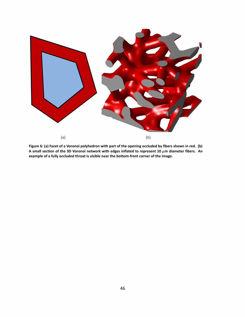
46

Figure 6: (a) Facet of a Voronoi polyhedron with part of the opening occluded by fibers shown in red. (b) A small section of the 3D Voronoi network with edges inflated to represent 10 m diameter fibers. An example of a fully occluded throat is visible near the bottom-front corner of the image.

47

Figure 7: Various size distributions arising from the Voronoi network construction.

48

Figure 8: 3D images of water invasion into Voronoi fiber networks simulated using the modified image morphology approach. (a) and (b) show the invasion pattern at different applied pressures with fibers removed for clarity. (c) shows a full network image including fibers (white) and water (blue).

49

Figure 9: Comparison of experimental mercury intrusion capillary pressure data with curves modeled by various methods.

50

Figure 10: Comparison of experimental water injection capillary pressure data with curves modeled by various methods.

51

Figure 11: Invading fluid configurations (blue) in the pore network predicted by the invasion percolation algorithm stopped at the point of breakthrough. (a) 3D perspective with the top and bottom fiber outline shown for reference, (b) side view showing the percolating finger more clearly, and (c) saturation profile at the point of breakthrough (total saturation was 19.87%).

52

Figure 12: Water percolation into the pore network (blue) and resulting oxygen concentration distribution (indicated by color according to the color scale). The foremost corner has been removed to show internals and fibers have not been drawn for clarity. Note that the O2 concentration is fairly uniform and high (white) throughout the domain due to a flux bottleneck at the injection face.

53

Figure 13: Relative effective diffusivity (DEFF(SNWP>0) / DEFF(SNWP=0) of the network model as a function of invading fluid saturation as determined using the ALOP algorithm. Inset: Normalized effective diffusivity (DEFF(SW>0) / DAB). Fluid invaded from the Z face in the through-plane direction. Note that the reported fluid saturation include the late pore filling model, so saturations are less than if the pores were completely filled upon invasion.

54

Figure 14: Throat orientation as defined by the unit normal vector of the facet. Left: Distribution of X-components (red) and Z-components (blue) of throat normal vectors. Throat facets oriented in the XY plane due to anisotropy have a Z-component approaching 1. Right: The relationship between throat orientation and size. The anisotropy in the network has very little influence on the actual size of throat facets.