Several aspects of three-dimensional Delaunay triangulation

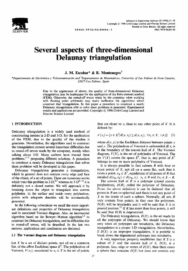
ELSEVIER

Advances in Engineering Sofware 21 (1996) 21-39 Copyright 0 1996 Civil-Comp Limited and Elsevier Science Limited

Printed in Great Britain. All rights reserved SO965-9978(96)00006-3 0965-9978/96/%15.00

Several aspects of three-dimensional Delaunay triangulation

J. M. Escobar” & R. Montenegro? *Departamento de Electrdnica y Telecomunicacidn and ?Departamento de Matembticas, University of Las Palmas de Gran Canaria,

3.5017-Las Palmas, Spain

Due to the appearance of slivers, the quality of three-dimensional Delaunay triangulation may be inadequate for the application of the finite-element method (FEM). Otherwise, the round-off errors made by the computer when working with floating point arithmetic may make ineffective the algorithms which construct that triangulation. In this paper a procedure to construct a nearly Delaunay triangulation able to solve these problems is presented. Experimental results and applications are provided. Copyright 0 1996 Civil-Comp Limited and Elsevier Scie& Limited -

1 INTRODUCTION

Delaunay triangulation is a widely used method of constructing meshes in 2-D and 3-D, for the application of the FEM, due to the quality of the meshes it generates. Nevertheless, the algorithms used to construct the triangulation present several important difficulties due to round-off errors made by the computer, mainly when talking about 3-D. Many authors have treated these problems,‘-’ proposing different solutions. A procedure to construct a nearly Delaunay triangulation that solves these problems will be developed in this paper.

Delaunay triangulation generates a triangulation, which in general does not contain every edge and face of the object, of a set of points. There are numerous works which treat this problem in 2-D,6*7 whereas in 3-D8-” it is definitely not a closed matter. We will approach it by breaking down the object to triangulate into convex polyhedra. In the surface and inside every polyhedron, points with adequate densities will be automatically generated.

In the following subsections we recall the more important deIinitions and properties of Delaunay triangulation and its associated Voronoi diagram. Also, an incremental algorithm based on the Bowyer-Watson algorithm”* to construct the Delaunay triangulation, and its difhculties due to round-off errors, wiIl be described. In the last two sections, applications and conclusions are discussed.

1.1 The Voronoi diagram and Delaunay triangulation

Let X be a set of distinct points, not all on a common flat, of the affine Euclidean space E3. The polyhedron of Voronoi, I’(.*-,), associated to xi E X is the set of points

that are closer to xi than to any other point of X. It is defined by:

V(x;) = {x E E3/d( X, Xi) < d(X, Xj), VXj E X, i #j} (1)

where d(x, y) is the Euclidean distance between points x and y. The polyhedron of Voronoi is unbounded iff Xi is in the boundary of the convex hull of X. The Voronoi diagram, V(X), is the set of polyhedra of Voronoi. The set V(X) covers the space E3, that is, any point of E’ belongs to one or more polyhedra of Voronoi.

It is always possible to find subsets R with four or more points of X, not all on a same flat, such that it exists a point, vR E E3, equidistant of all points of R that satisfied d(UR,Xk) < d(UR,Xi), xk E R and VXi E x - R.

The convex hull of R is a polytope (closed convex polyhedron), D(R), called the polytope of Delaunay. From the above definition it can be deduced that all points in R are co-spherical and there is not any point of X in the inside of such a sphere. Normally, all sets R only contain four points; in that case the polytopes, D(R), will be tetrahedra and it will be said that X is in general position.‘* If R has more than four points, it will be said that D(R) is degenerated.

The Delaunay triangulation, D(X), is the set made by all the polytopes of Delaunay. We should know that only when all polytopes are tetrahedra, the Delaunay triangulation is a proper 3-D triangulation. Nevertheless, if D(X) is an improper triangulation, it is possible to break down the degenerated polytopes into tetrahedra.

A very important property establishes that if S is a subset of X and the convex hull of S, D(S), is a polytope, face, edge or vertex of D(X), then there exists a sphere that contains D(S) but does not contain any

27

28 J. M. Escobar, R. Montenegro

Fig. 1. The Voronoi diagram of 30 random points.

point of X - S. Reciprocally, if S is a subset from X such that there exists a sphere that contains D(S), but does not contain any point of X - S, then D(S) is a polytope, face, edge or vertex of D(X). We will refer to the aforementioned spheres as circumspheres. When D(S) is a polytope the circumsphere is a circumscribed sphere. This is a generalization of a property known as property of empty spheres.12?13

It is convenient to have a local characterization of the Delaunay triangulation. Let S and S’ be subsets of X such that D(S) and D(S’) are two opposite polytopes. It is said that the polytopes are locally Delaunay if both have circumspheres B and B’, and S’ - S is outside B (equivalently, S - S’ is outside B’). A triangulation T is locally Delaunay if every pair of opposite polytopes is locally Delaunay. A triangulation is Delaunay iff it is locally Delaunay. l2 Figures 1 and 2 display the Voronoi diagram and Delaunay triangulation of 30 random points.

Fig. 2. The Delaunay triangulation of 30 random points.

1.2 An incremental algorithm to construct the Delaunay triangulation

The incremental algorithms construct triangulations by adding points one by one. We are going to describe an incremental algorithm which constructs a proper Delaunay triangulation. It is based on the Bowyer- Watson algorithm1P2 and modified by other authors like Cavendish,3 George,’ etc. The main points are:

1.2.1 Initial triangulation The algorithm is simplified if we construct an initial tetrahedron, TO, or a broken-down-into-tetrahedra prism that contains all points of X.

1.2.2 Addition of Xi+, in the triangulation Suppose the triangulation D(Xi) of the first i points is already done. The set Di of tetrahedra whose circumscribed spheres contain xi+ i, is found.

Di = { Tj E D(Xi)/Xi+ 1 E B( Ti)} (4

Let C’n, be boundary faces of D{, that is, faces that only belong to one tetrahedron of 0;.

The triangulation D(Xi+ i) that includes point Xi+ i is defined by:

D(Xi+ 1) = (D(Xi) - 0:) U 0: (3)

where 0; = Uj{C’, Xi+ 1) is the set of tetrahedra formed by the point xi+i and the face C’ and C’n,. If the circumspheres of tetrahedra of D{ are exactly evaluated, the tetrahedra from 0: are well constructed. The reason is that faces,of C’n, are visible with regard to xi+ 1, that is to say, Di is star-shaped with regard to xi+ 1.

As an example, Fig. 3 shows the triangulation of Xs = {Xl,... , xs} (bold lines) and the resulting triangulation when x9 is added. The boundary faces of 0; =

are c& = {C,, . . . , C6}. Tetrahedra

Fig. 3. Addition of x9 in the triangulation.

3-D Delaunay triangulation 29

X2 X2 (cl (4

Fig. 4. Different possibilities about the triangulation of X = {xi, . . . , x5} due to round-off errors.

formed with x9 and the faces of C’,-,, are depicted with dashed lines.

1.3 Problems due to round-off errors

When X is not clearly in a general position, some problems due to round-off errors can break down the algorithm. We are going to show some of these problems.

Suppose X = {xi,. . . ,x5} is a set of five co-spherical points of E2 (the situation is analogous to E’) and triangles T, = (x1, x2, x3} and T2 = {x1, x3, x4} are formed with the first four points, Depending on the computed position of x5, the four possibilities that can happen are:

(1) If the computer evaluates that x5 E B(TI) and x5 $ B( T2), the process removes T, and retains

(2)

(3)

(4)

T2. The new triangles, (x1, x2, x5} and (x2, x3, x5}, are created (Fig. 4a); If the computer evaluates that x5 $ B(TI) and x5 E B( T2), the process retains T, and removes T2. The new triangles, {xt,x3,x5} and {x3,x4, x5}, are created (Fig. 4b); If the computer evaluates that x5 E B(T,) and x5 E B(T2), the process removes T, and T2. The new tfiangles, {XI, x2,x31, (~2, x3, -3) and (~3, ~4, x5} are created (Fig. 4c); If the computer evaluates that x5 $ S( T,) and x5 6 B( T2), the process retains T, and T2. The new triangle, {xi, x4, x5}, is created (Fig. 4d).

All possibilities are admissible except (1) because edge x1x3 is not visible with regard to x5. It is said that a cross between tetrahedra is produced.

Another troublesome case, which only happens in 3-D (or greater than 3), is the appearance of sliver tetrahedra. Suppose that in X = {xi, . . . , x6} points x1, x2, x3 and x6 are on the same circumference and the tetrahedra T, = {xI,x2,x3,x4} and T2 = {xI,x2,x3,x5} have been constructed before adding x6. Depending on the computed position of x6, the four possibilities that can happen are:

If the computer evaluates that x6 E B(Tl) and x6 q’ B(T,), the process removes T1 and retains T2. The new tetrahedra, {x1,x2,x3,x6}, {x1,x3, x4,x6)? {x2?x3?x47x6) and {X1jX2!X5rX6) are created (Fig. 5a); If the computer evaluates that x6 $! B( T,) and x6 E B( T,), the process retains T, and removes T2. The new tetrahedra, {x1,x2!x3,x6), {xtrx3, x5,x6), {~2~X3~xS~x6~ and fxITx2,x4~x6) are created (Fig. Sa); If the computer evaluates that x6 E B(TI) and x6 E B( T2), the process removes T, and T2. The new tetrahedra, {x17x3~~5~x6}~ {x2?x37x57x6}T

{x1,x3,x4,x6} and {x2,xJ,x4,x6} are created (Fig. 5b); If the computer evaluates that x6 $ B( T,) and x6 8: B( T,), the process retains T, and T,. The

Fig. 5. Different possibilities about the triangulation of X = (x1, . ! ,Q}.

30 J. A4. Escobar, R. Montenegro

new tetrahedra, {xi, x2, x5, x6} and {xi, x2, x4, x6} are created (Fig. 5~).

Situations (1) and (2) (Fig. 5a) are inadmissible because the tetrahedron {x1, x2, x3, x6} is sliver (null volume). Furthermore, if x6 is under the plane defined by x1, ~2 and ~3, and the round-off errors allow situation (1) to happen, face {xi, x2, x3} will not be visible with regard to x6. It appears to be a cross between tetrahedra. (A similar problem can happen if in situation (2) x6 is over the plane.) The other situations are admissible. It should be noted that even with an exact evaluation of the position of the new point, some situations can be reached in which arbitrary flat tetrahedra are constructed. It should be sufficient that point x6 was situated, for example, on the surface of B(Tt) and over the flat determined by points x1, x2 and x3. From a FEM point of view, the triangulations of Fig. 5(b), (c) are preferable, even if they are not strictly Delaunay ones.

2 CONSTRUCTION OF D(xi+l)

The most critical part of the above algorithm is to search a set D{ such that the resulting triangulation D(Xj+,) is admissible. Triangulation D(Xi+l) will be admissible if set 0: has admissible tetrahedra.

It will be said that a face C E C’n, is +visible if it is visible with regard to xi+t, and it happens that:

where n is the unitary and perpendicular to face C vector projecting from 0:. This minimum occurs when x is a vertex of face C. A closed polyhedron will be said to be e-star-shaped if all its faces are e-visible.

To construct a set 0: with admissible tetrahedra, we must require that 0: should be e-star-shaped with a large enough parameter E. The strategy used to do

so will be to find the tetrahedron or set of tetrahedra, kernel, that contains Xi+i and from it to extend the kernel with certain controls until 0; is completed.

2.1 Search for the kernel

Let us suppose that triangulation D(Xi) of the first i points of X has already been constructed. The search for the kernel starts in some of the tetrahedra of D(Xi). Obviously, the search is shorter if the tetrahedron from which we start is near point xi+i. If there is no information that allows us to connect the number allocated to each tetrahedron with its space position, it cannot be known a priori whether the tetrahedron is near or far from xi+i. Nevertheless, due to the orderly way in which the points of X have been defined, it is probable that point xi+i is usually near the last tetrahedron included in D(Xi). We will choose this last tetrahedron, T,,, to start the search for the kernel from. An alternative to the orderly point insertion is the random order insertion (random incremental algorithm). In this case the number of tetrahedra that have to be traversed to find the kernel is greater, but the number of tetrahedra belonging to Df is less. The CPU time is usually favourable when the point insertion is made in an orderly way, as has been experimentally checked in many applications. Some data related to these topics are provided at the end of this paper.

The search algorithm consists in moving from a tetrahedron T to the adjacent one, T,,, that is in the direction of the straight line joining T with xi+,. The success of this procedure is guaranteed as the set of tetrahedra is a convex set, and the adjacent tetrahedron mentioned above is therefore always found.

The SEARCH procedure takes charge of finding one of the kernel tetrahedron. The KERNEL procedure takes charge of finding the rest, if there are any. Figure 6 shows the search for the kernel.

(a> lb) Fig. 6. Search for the kernel.


Fig. 7. Kernel formed by (a) one, (b) two or (c) more tetrahedra.

2.1 .l Kernel search algorithm procedure SEARCH input: D(Xi), T,,, Xi+l; output: N’, EN

T:= T, end : = false

repeat if(n - Y 5 0, VC E T) then (where v is a unitary vector in the direction from face C to xi+ 1 and II is the unitary, perpendicular to face C and projecting from T vector) (the tetrahedron T belongs to the kernel)

procedure KERNEL input: D(Xi), T, q+l; OUtpUt: N’, EN

end: = true else

the face C that maximizes n-v is found (C is the face that “best sees xi+i”) the tetrahedron T, # T/C E T, is found T := T, (it passes through neighbouring tetrahedron)

end if until (end = true) end procedure

The search for the kernel is done by moving from tetrahedron T to tetrahedron T, through the face C that minimizes the angle (maximize II * v) formed by vectors n and v. When T belongs to the kernel, every amount II. v is negative or null. The KERNEL procedure locates the set of tetrahedra of the kernel from one of them, and it determines the,parameter eN from which the kernel is E- star-shaped. In Fig.7 the different situations analyzed by the KERNEL procedure are shown.

To assure that the kernel is e-star-shaped for an accept- able 6, the KERNEL procedure considers that Xi+ r is on a face or edge when actually it is at a small distance much shorter than the distance between points of X.

2.2 Setting of D{

Set 0: must satisfy three fundamental requirements:

(1) a tetrahedron T belongs to D{ only if xi+ t E B(T) (2) set D\ must be c-star-shaped with regard to xi+l. (3) set Df must not contain any other point of X

apart from Xi+ 1.

SET 0; algorithm described below satisfies the first two requirements. Later, we shall show how to satisfy the last. Tetrahedra whose circumspheres contain Xi+l

and are adjacent to actual D{ set, are stored in ND;. SET Di algorithm makes a series of iterations in each of which it adds this set to Df . When NDf is empty, the algorithm analyzes if D{ is c-star-shaped. If it is so, 0; has been set and the algorithm stops; else, set of tetrahedra T, belonging to D{ which has any face not e-visible with regard to xi+, are found. The radius of these tetrahedra are considered as null to prevent these tetrahedra from being again included in D’, and the algorithm from starting again. If when the algorithm analyzes whether D{ is c-star-shaped there are many tetrahedra of T, also belonging to the kernel, the actual value of e is too much restrictive to construct a set 0; e-star-shaped. It must be changed by EN, which will be smaller. Once it has been done the algorithm starts again. A more conservative choice is to change E by a decreasing sequence of values of ci, such that EN 5 ei < E. This choice probably constructs sets Df better shaped, but it takes it longer to converge.

(4 (b)

(4

Fig. 8. Different steps of the algorithm SET 0:.


(a) (W

Fig. 9. (a) Round-off errors allows that Xj is contained in 0;; (b) any point except Xi+, is contained in Df .

In Fig. 8 the main steps are represented used by SET 0; algorithm for the determination of 0;.

(1)

(2)

(3)

(4)

The kernel, N’ = { Ti} and the set of tetrahedra {Tl,..., T5} whose circumspheres contain xi+1 admitting possible round-off errors; The kernel is extended until it becomes Di = {TI, T2, T3, T4);

Current set 0; is not e-star-shaped with regard to %+I; for example, cos( Xi+lXv2, n) < 0; The algorithm starts again, Now, tetrahedron T4 is considered as if B( T4) does not contain xi+ 1, and that is why the algorithm stops once T3 has been added to 0:.

As can be seen in Fig. 8, it is not possible to determine an admissible set 0: only by taking out tetrahedron T4 from {Tl,..- , T5}, as the outcoming set would not be connected.

2.2.1 Algorithm of construction of 0; If we consider B’ = (B(T)/T E D(Xi)} and Rqq is the radius of B(T), the algorithm can be summarized as follows:

procedure ,SET 0: input: D(Xi), B’, N’, xi+l, E, EN; output: D’l

D; := N’ set NDj = {T adjacent to N’/Xi+ i E B(T)} is found

while (ND\ # 8) do 0; := 0; U ND; (set Di is actualized) set ND; = {T adjacent to 0; /xi+ i E B(T)} is found

end while if (Df is not e-star-shaped with regard to xi+,) then

set C,,, = {C E boundary of Di/C is not e-visible} is found set T, = {T E 0: /any face of T E C,} is found

if (3T E T,,, n N’) then (the actual value of e is

too much restrictive. It is changed by EN, which will be smaller)

e:= EN SET Di input: D(Xi), B’, N’, xi+], E, CN; output: D{ (the algorithm is started again with a smaller c parameter)

else RBcT) := 0, VT E T,, (it avoids that tetrahedron .T is again included in pi) SET 0; input: D(Xi), B’, N’, xi+l, e, EN; output: 0: (the algorithm is started again with null radii of “circumscribed spheres” of set T,)

end if end f

the initial values of those radii which have been modified during the process are now restored

end procedure

If the round-off errors in the evaluation of the

Fig. 10. Point generation on faces.


circumspheres of the tetrahedra of 0: are similar to the distance between points of X, the procedure above does not assure that any other point of X, apart from xi+ r, is contained in 0:. In Fig. 9(a) this possibility is shown, in 2-D.

To avoid this situation the incircle test in SET Df is calculated by using the minimum radius of B( T) , that is to say:

(5)

where uj is the j-esime vertex of the tetrahedron T and cr is the centre of B(T).

In spite of the imprecision in the calculation of the centres and radii of the circumspheres (solving a 3 x 3 linear system by Gaussian elimination using complete pivoting), it will be impossible that Di contains any point apart from xi+ i (see Fig. 9b). In a real situation, if we work with double precision and distances between points are not too small, it is really difficult that the

Fig. 11. (a) Global, (b) surface and (c) object triangulation.


situation mentioned above occurs. Specifically, the maximum observed difference between maximum and minimum values of d(cr,q), 1 li 5 4 in several applications has been about lo-l2 with a minimum distance between points close to lOi.

More detail of these algorithms can be found in Ref. 14.

2.3 Setting of 0:

This phase of the program depends on the type of data structure that it is used. In our code we store the tetrahedra, faces, edges and points of the triangulation and the connectivities between these elements. That is to say, when point xi+i is included in the triangulation to form D(Xi+l) we need to update the numbers of tetrahedra, faces and edges (points are not modified). The sets of tetrahedra, faces and edges that disappear when Xi+ 1 is added are named D:, Cl, and Ai respectively. The sets of tetrahedra, faces and edges of D(Xi+l) tO which Xi+i belongs are named Di, Ci and A$, and the boundary faces, edges and points are named C’u,, AjD, and V$,,. These sets are calculated from set Di using the stored data of the triangulation.

Set 0: is formed by point xi+ i and the boundary faces C’o, of Di, set C$ is formed by point xi+ r and the boundary edges A;,-,,, and set Ai is formed by point Xi+ i and the boundary points (there are only boundary points in Di) Vjo,.

Once these sets have been determined, the connectivities are restored.

3 OBJECT DEFINITION AND POINT GENERATION

In order to check our triangulation algorithm, an input data and a point insertion strategy have been designed capable of generating meshes of relatively simple objects, and which are obviously improvable by using, for example, CAD systems. Nevertheless, some ideas used for the design of them both are presented here. The object to be triangulated, R, is defined by points distributed inside it and on its surface. The points must be placed in such a way that the triangulation of the object, T(R), is a subset of D(X), where the set of points X includes the points that define the object and the points belonging to the initial broken-down-into- tetrahedra prism. If the above condition is satisfied, we say that the triangulation is boundary conforming.g9’0 In this case, T(0) is obtained by subtracting from D(X) the tetrahedra not belonging to Q. The shape of T(R) is polyhedral; therefore, only polyhedral objects can be exactly represented. All points of a, except its vertices, are automatically generated. To simplify the generation of points, the 0 object is broken down in convex polyhedra. A convex polyhedra is defined by its faces,

the faces are defined by its edges, and the edges by its extreme points. The code generates points, at a suitable distance from the boundary, in the relative inside of each edge, face and convex polyhedron. The distance

Fig. 12. (a) Surface and (b) object triangulation; 7046 points and 30141 tetrahedra.


N: ” t m

bX

erh e

ud f:

26000

20000

15000

10000

so00

0 1 17 A 93 177

OQ-20 2O-!P 50-100 loa-2o" 20'300

Degrees

Fig. 13. Mesh measure quality.

between points in each element is previously specified in the input data. The above strategy in point generation does not guarantee that the triangulation is boundary conforming. If in the decomposition of the object in convex polyhedra we have some vertices, edges or faces of different polyhedra close between them, the edges or faces of polyhedra can be removed. To avoid this problem we can adjust the density of points on these edges and faces.

The input data consists of one table with the number of each vertex and its coordinates, another table with the number of each edge and the numbers of its extreme points, another one with the number of each face and the numbers of its boundary edges, and a final one with the number of each polyhedron and the numbers of its boundary faces.

3.1 Point generation in edges

The distance 6, between inner points of an edge A is specified in the input data. The code adjusts this distance such that the distance between inner points is the same as the distance between an extreme point and the adjacent inner one.

3.2 Point generation on faces

In Fig. 10 two confluent and no parallel edges of the face are considered in order to construct two unitary and linearly independent vectors u1 and u2 in such directions. The inner points are generated in directions u1 and u2 with specified distances between them and a suitable distance to boundary edges. The point of intersection of the two edges can be chosen by the user. In general, this

point is chosen in such a way that the angle formed by u1 and u2 is as close to 7r/2 as possible.

Let 6, be the distance between points in edge A belonging to faces C, and q&+1 any segment of A formed by two consecutive points. If the distance dA from the inner points of two faces to common edge A is greater than l/26*, then there exists a circumsphere of x&+ 1 that does not contain any inner point of these faces. Therefore, edge A is not removed by the inner points of these faces. A similar procedure is done with all of the edges of C.

In Fig. 10 we can see that inner points of C are generated in the directions u1 and u2 with distances 6, and 6, between them, respectively. The minimum distance to edge A is greater than l/28*. Distance dA between point x and edge A can be evaluated as: dA = I(v x n) -%I been n = u1 x u2/IIu1 x ~~11 the unitary and perpendicular to C vector and v = xgx,/IIxbx,II, where xb and x, are the extreme points of A attending to the criteria showed in Fig. 10. Point x is in the inside of Ciff(vxn)-q>O,VAEC.

3.3 Point generation in polyhedra

Three confluent and no parallel edges of the polyhedron are considered in order to construct three unitary and linearly independent vectors ul, u2 and u3 in such directions. The inner points in the polyhedron P are generated in directions q, u2 and u3 with specified distances between them and a suitable distance to the boundary faces.

It can be showed that an upper bound for the largest empty circle in face C is a circle with radius r =


9/3Zj + max&J), where 15,~ is the distance C and its edges are not removed by the inner points of between generated points in edge Ai belonging to C, and these polyhedra. 6i and 6, are the distances in the directions u1 and u2, The distance dC between point x and face C belonging respectively, between inner points of C. to polyhedron P can be evaluated as: d, = (Xx, - ~1,

If the distance dc from inner points of two polyhedra where n is the unitary, perpendicular to C and projecting to common face C is greater than r, it can be assured, from P vector, and x, is any vertex of C. Point x is inside attending to the property of empty spheres, that the face PiIf%-n>O,VCEP.

110

t IOU

i

i 70

co 00

P u: s0

C 40

0 30

n

d 20

S 10

0

t

i m e

i Cn P US

e C

0

n d s

IO00 2000 2060 4000 5000 6000 7000 8060 9000 10000 11.80 I2006 12000 14060 15066 16000 17000 18006 19000

Number of points

(a) 110

I.0

90

so

70

66

I

46

30

7.4

IO

0

1.66 2wlO 3lm 4660 so00 6000 7Ooe am0 9600 16008 ll6.e llew 12.w 14we mm 16.60 17Bw 18686 19006

Number of points

(b) Fig. 14. CPU time vs number of points, (a) without, and (b) with randomness. Average number of tetrahedra crossed to find the

kernel vs number of points, (c) without and (d) with randomness.


4 APPLICATIONS

Several applications using our 3-D mesh generator are presented in this section. As a first example, Fig. 11 shows the 3-D triangulation of a simple object formed by three convex polyhedra. In Fig. 11(a) the global triangulation including points of the initial prism, points on a spherical surface between the prism and the object and, finally, the points of the object are shown. Points on a spherical surface are not strictly necessary, but we obtain a better quality of tetrahedra formed during the triangulation process decreasing round-off errors. In Fig. 1 l(b), the triangulation of

the object surface is shown. Finally, the corresponding 3-D triangulation is presented.

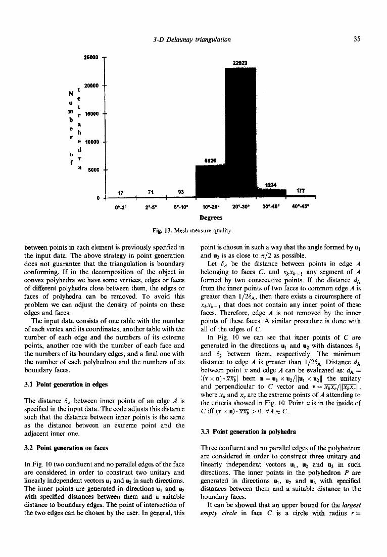
A more complex application can be observed in Fig. 12: surface (a) and 3-D triangulation (b). The number of points in this object is 7046 and the number of tetrahedra is 30141.

The mesh measure quality of a tetrahedron T can be given by tin1 sps4{+p}, where

& = sen-‘(1 - cos2 ap - cos2 pp - cos2 7,

+ 2 cos c$ cos pp cos yp)‘12 (6)

and CQ,, BP and 7, are the flat angles in vertex p. The

loo0 2ooa r3Lxo 4lxo 5om fsow 7aJo 8ooo sow 1Mxx)11ooo12oool3wo14oM)15oooleooo17ooo18oM)19ooo

Number of points

(c)

loo0 2l.m moo 4oc4l 5mo eooo 7ow sow eax,loooorl~lmoo13oao14wolsoooleooo1700018000180M)

Number of points

(4

Fig. 14. Continued.


(b) I

Fig. 15. (a) Object with surfaces and (b) lines crossing them inside it.

value of 4 is 45” for an equilateral tetrahedron and 0 for a flat one. Figure 13 shows the mesh measure quality of the object. These results have been obtained without using any smoothing methods.

CPU time in seconds, on a HP-730 workstation, vs the number of points introduced in the triangulation are presented in Figs 14(a), (b), without and with randomness, respectively. Approximately a linear complexity in function of the number of points is obtained. In Fig. 14(c), (d) the average number of tetrahedra that

have to be crossed until the kernel is found vs the number of points included in the triangulation, without and with randomness is shown. When there is not randomness, the kernel search starts from the last tetrahedron included in the triangulation, and when there is, it starts from the no. 1 tetrahedron. The average number of tetrahedra belonging to set Di is somewhat greater when there is not randomness (20.75) than when there is (17.76). This explains that the CPU time is smaller, in spite of the kernel search taking longer with randomness than without it.

We can find applications in which several surfaces and edges, crossing between them inside the object, must be respected. As we said previously, this problem can be solved adjusting the densities of the generated points in the object. The example of Fig. 15 shows three lines and two surfaces (b) located in the triangulation of the object (4.

5 CONCLUSIONS

The procedure used to construct the Delaunay triangulation, or at least a nearly one, has been proved in numerous applications and obtained good results. One of the advantages of this method is that it does not need to use an exact arithmetic in the computation. This results in a saving of CPU time and of memory. In experimental results we have obtained approximately a linear complexity in function of the number of points.

On the other hand, the object is characterized by the points automatically generated on its surface and inside; a previous triangulation of its surface is not necessary. In future works we will try to improve the automatic points generation for more complex objects. Based on our experience in 2-D nested meshes,15 in the future we will try to combine this 3-D mesh generation with a refinement/derefinement algorithm.

ACKNOWLEDGEMENTS

This research has been sponsored in part by AHEMON, S.A. through the Foundation of the University of Las Palmas de Gran Canaria.

REFERENCES

1. Bowyer, A., Computing Dirichlet tessellations. Comput. J., 1981, 24(2), 162-166.

2. Watson, D. F., Computing the n-dimensional Delaunay tessellation with application to Voronoi polytopes. Comput. J., 1981, 24(2), 167-172.

3. Cavendish, J. C., Field, D. A. & Frey, W. H., An approach to automatic three-dimensional finite element mesh generation. Znt. J. Numer. Meth. Engng., 1985, 21, 329- 347.


4. Perronnet, A., Un algorithme de tetraedrisation d’un objet multi-materiaux ou de l’exteriour d’un objet. Publications du Laboratoire D’Analyse Numerique, Paris, 1988.

5. George, P. L. & Hermeline, F., Delaunay’s mesh of a convex polyhedron in dimension d. Application to arbitrary polyhedra. Znt. J. Numer. Meth. Engng., 1992, 33,975-995.

6. Weatherhill, N. P., The integrity of geometrical boundaries in two-dimensional Delaunay triangulation. Commun. Appl. Numer. Meth., 1990, 6, 101-109.

7. Friedish, O., A new method for generating inner points of triangulations in two dimensions. Comput. Meth. Appl. Mech. Engng., 1993, 104, 77-86.

8. George, P. L., Fully automatic mesh generator for 3-D domains of any shape. Impact Comput. Sci. Engng., 1990, 2, 187-218.

9. George, P. L., Hecht, F. & Sahel, E., Automatic mesh generator with specified boundary. Comput. Meth. Appl. Mech. Engng., 1991,92, 269-288.

10. Weatherhill, N. P. & Hassan, O., Efficient three- dimensional grid generation using the Delaunay triangulation. Comput. Fluid Dyn., 1992, 2, 961-968.

11. Johnston, B. P. & Sullivan, J., A normal offsetting technique for automatic mesh generation in three dimensions. Znt. J. Numer. Meth. Engng., 1993, 36, 1717-1734.

12. Fortune, S., Voronoi Diagrams and Delmmay Trknguiations. Computing in Euclidean Geometry. World Scientitic, Singa- pore, 1992.

13. Preparata, F. P. & Shamos, M. I., Computational Geometry: an Introduction. Springer, New York, 1985.

14. Escobar, J. M. & Montenegro, R., Several aspects of the three-dimensional triangulation of Delaunay. In Advances in Post and Preprocessing for Finite Element Technology. Civil Comp Ltd., Edinburgh, 1994, pp. 193-204.

15. Ferragut, L., Montenegro, R. & Plaza, A., Efficient refinement/dere!&ment algorithm of nested meshes to solve evolution problems. Commun. Numer. Meth. Engng., 1994, 10,403-412.

Several aspects of three-dimensional Delaunay triangulation

Documents

Transcript of Several aspects of three-dimensional Delaunay triangulation