Application of Delaunay triangulation to the nearest neighbour method of strain analysis

Application of Delaunay triangulation to the nearest neighbour

method of strain analysis

Kieran F. Mulchrone*

Department of Applied Mathematics, National University of Ireland, Cork, Republic of Ireland

Received 11 October 2001; accepted 14 May 2002

Abstract

The nearest neighbour method of strain analysis is re-evaluated and a method for objectively determining nearest neighbours, namely the

Delaunay triangulation, is applied. A simulation study and application to a real set of data demonstrates that this approach makes the NNM of

strain analysis a practical (and computationally more efficient) alternative to the Fry and associated methods. Once nearest neighbours are

selected centre–centre distances can be processed by normalisation and enhancement and the best fit ellipse is determined using a steepest

gradient non-linear least squares algorithm applied to the polar equation of a centred ellipse. A simulation study indicates that the technique is

a valid one and estimates the strain ellipse well at the 95% confidence interval. Application to a set of natural oolite data shows that there is a

systematic variation of error with selection factor and it is suggested that the best estimate of the strain ellipse is obtained by choosing the

selection factor which minimises the error.

q 2002 Elsevier Science Ltd. All rights reserved.

Keywords: Strain analysis; Nearest neighbour; Delaunay triangulation

1. Introduction

Ramsay (1967, p. 195) introduced the idea that finite strain

may be estimated using the distance between centres of

adjacent objects, provided the objects were evenly distributed

prior to deformation. Implementation of this technique in two

dimensions involves determining nearest neighbours, calcu-

lating the distance between nearest neighbours (di ) and the

orientation of the line joining them (fi ). Subsequently by

plotting di against fi, the minimum and maximum averaged

values of di (dmin and dmax) could be estimated and divided to

provide an estimate of ellipticity R. The orientation of the

extensional axis of the strain ellipse is taken to parallel the

orientation of dmax. Strain may also be estimated by

determining the best-fit least-squares ellipse for the data

(Ramsay and Huber, 1983, p. 117; Erslev and Ge, 1990; Hart

and Rudman, 1997). Although the nearest neighbour method

(NNM) has been shown to work, there are several problems

associated with it (Erslev, 1988):

1. No exact definition of what constitutes a nearest neighbour

leading to subjectivity in measurement.

2. Difficulties with interpretation.

3. Labour intensity.

As a result there has been minimal application of the

Ramsay’s NNM.

Graphical methods of strain analysis, which utilise all

object–object separations, such as Fry’s Method (Fry, 1979),

the Normalised Fry Method (Erslev 1988) and the enhanced

Normalised Fry Method (Erslev and Ge, 1990) have super-

seded the NNM due to their simplicity and easy application.

In addition, McNaught (1994) extended these methods for

application to aggregates of non-elliptical objects. More

recently these methods have been incorporated into auto-

mated computer based analysis tools including automatic

image analysis applications (Aillieres and Champenois, 1994;

Aillieres et al., 1995). Although these methods are graphi-

cally simple, they are computationally expensive and are of

O(N 2), i.e. to process N data takes approximately N 2 steps.

In this paper the NNM is revisited in the context of the

relatively new subject of computational geometry. The

object of this paper is to demonstrate that the NNM readily

lends itself to analysis by the methods of computational

geometry such as Delaunay triangulation and that the finite

strain may be determined by statistical analysis of the

resulting data. In order to distinguish between Ramsay’s

0191-8141/03/$ - see front matter q 2002 Elsevier Science Ltd. All rights reserved.

PII: S0 19 1 -8 14 1 (0 2) 00 0 67 -6

Journal of Structural Geology 25 (2002) 689–702

www.elsevier.com/locate/jstrugeo

* Tel.: þ353-21-902378; fax: þ353-21-270813.

E-mail address: [email protected] (K.F. Mulchrone).

http://www.elsevier.com/locate/jstrugeo

NNM and that developed here, the current method will be

referred to as the DTNNM (standing for Delaunay

triangulation nearest neighbour method). Use of the

Delaunay triangulation and statistical analysis removes

subjectivity in measurement and interpretation. Further-

more, the DTNNM is computationally more efficient by

comparison with the various Fry methods (Fry, 1979;

Erslev, 1988; Erslev and Ge, 1990; McNaught, 1994). This

is because calculating a Delaunay triangulation is O(NlnN )

in the worst case (Perparata and Shamos, 1985, p. 123;

Edelsbrunner, 1987, p. 305; O’ Rourke, 1993, p. 200; Huang

and Shih, 1998), i.e. it is 50 times faster for 100 data and 300

times faster for 1000 data. In addition it also automatically

selects a subset of nearest neighbours. The difference

between an O(N 2) and an O(NlnN ) algorithm is not an issue

on most modern personal computers for a typical geological

dataset; however, it may be an issue for large datasets or

collections of datasets particularly in the light of the

development of automated image analysis techniques

(Aillieres and Champenois, 1994; Aillieres et al., 1995).

2. Delaunay triangulation, Voronoi diagram and convex

hull

A Delaunay triangulation is the set of lines joining a set

of points together such that each point is joined to its nearest

neighbours (Perparata and Shamos, 1985, p. 209; O’

Rourke, 1993, p. 175). Before elaborating further on

Delaunay triangulations, it is instructive to consider a

closely related property of a set of points, namely the

Voronoi diagram. Consider a set of n nodes P ¼ {p1, p2,

p3,…,pn} (see Fig. 1a for an example set) and that the plane

is partitioned by assigning every point in it to its nearest

Fig. 1. (a) An example set of 10 points P ¼ {p1, p2,…,p10} in the plane. (b) When creating a Voronoi diagram the plane is partitioned by assigning every point

in the plane to its nearest neighbour. In this subset of points the arbitrary point p is nearest to p2. In constructing a Voronoi diagram every point in the plane is

assigned to its nearest neighbour, points with more than one nearest neighbour form part of the Voronoi diagram. (c) The Voronoi diagram corresponding to the

example set of points. (d) The Delaunay triangulation of the example set of points.

K.F. Mulchrone / Journal of Structural Geology 25 (2002) 689–702690

neighbour in P, for example in Fig. 1b the point p is assigned

to the node p2, its nearest neighbour. All points whose

nearest neighbour is pi form a region of the plane termed a

Voronoi region denoted by V( pi ) (see Fig. 1c). Certain

points do not have a unique neighbour and may be equally

close to two or more nodes, all such points form part of the

Voronoi diagram and lie along the lines in Fig. 1c. A

Voronoi diagram consists of a set of adjacent straight-sided

polygons that divide the plane into regions of closeness to a

given node. Voronoi diagrams have found many appli-

cations in diverse subject areas including crystallography

where Voronoi diagrams are used to simulate constant

crystal growth from dispersed sites of nucleation.

Once a Voronoi diagram has been devised, a Delaunay

triangulation may be superimposed by joining together

nodes, whose Voronoi regions touch, by a line (Fig. 1d). The

line joining the central nodes of two adjacent and toughing

Voronoi regions is the local shortest path between the two

nodes, because each Voronoi region consists of the points

which are closest to the central node. Many algorithms exist

which compute the Delaunay triangulation (Huang and

Shih, 1998) and Voronoi diagram of a set of nodes and the

interested reader is referred to O’ Rourke (1993) for a

thorough treatment.

A set of lines connecting nearest neighbours is the result

of computing a Delaunay triangulation. This is exactly the

information required to apply Ramsay’s NNM of strain

analysis. Because a Delaunay triangulation is calculated

computationally, it eliminates the time consuming and

subjective work that was previously associated with the

Ramsay’s NNM.

The convex hull of a set of points in two dimensions is

related to the above notions and is defined as the enclosing

convex polygon with the smallest perimeter and area (O’

Rourke, 1993, p. 70; see Fig. 2). The Voronoi diagram,

Delaunay triangulation and convex hull all have three-

dimensional counterparts so that the methods introduced

here for two dimensions can be quite easily applied to

higher dimensional problems.

3. Methodology

Objects used in the analysis are idealised as ellipses

mainly for computational convenience in the simulation

study and because the natural example studied consists of

elliptical objects. The primary prerequisite for both the Fry

method and the DTNNM is a set of points that were anti-

clustered prior to deformation and, equally important, that

the same set of points can be identified in the deformed

state. Fry (1979) chose to use object centroids for this

purpose, which are readily calculated for arbitrary shapes. In

general, it is not necessary to first approximate objects of

arbitrary shape by ellipses prior to application of the Fry

method or DTNNM (as suggested by Erslev and Ge (1990))

because the centroid of an arbitrary shape is as good (if not

better) a point as the centre of the fitted ellipse. Moreover,

although it may be computationally convenient to calculate

the enhancement factor (Erslev and Ge, 1990) for the

purpose of simulation using ellipse radii as described below,

these radii are readily calculable for arbitrary shapes also.

Therefore like the Fry method, the DTNNM applies to

objects of arbitrary shape.

The raw data required for the analysis is (ai, bi, xi, yi, fi ),

where ai and bi are the half-lengths of the long and short

axes of each ellipse, respectively, xi and yi are the co-

ordinates of the centre of each ellipse, fi is the orientation of

the long axis and i takes values between 1 and n, where n is

the total number of objects measured. Once the data is

acquired the following processing is applied.

Using centre co-ordinates (xi, yi ), the Delaunay triangu-

lation is calculated resulting in a data set D ¼ ((xi, yi ), (xj,

yj )). Both i and j take values between 1 and n and i – j (i.e. a

centre cannot be connected to itself). D represents the set of

connected nearest neighbours. As illustrated below with an

example (Fig. 4a), the Delaunay triangulation does not

always join nearest neighbours near the edge of the data set.

These rogue values may be eliminated by subtracting points

which form part of the convex hull from the Delaunay

triangulation (see Fig. 4b) and gives a modified Delaunay

triangulation (Dm ).

Dm is processed further by applying the enhancement of

Erslev and Ge (1990). The length (dij ) and orientation (uij )

of the line segment joining each pair of points (xi, yi ) and (xj,

yj ) are calculated. The length of the elliptical radius along

uij for each ellipse (ri and rj ) is calculated using the polar

Fig. 2. An example of the convex hull of a set of points. Notice that the hull

is everywhere convex and fully encloses the points in the set.

K.F. Mulchrone / Journal of Structural Geology 25 (2002) 689–702 691

equation of an ellipse centred on the origin, i.e.:

ei ¼

ffiffiffiffiffiffiffiffiffiffi1 2

b2i

a2i

sð1Þ

ri ¼ ai

ffiffiffiffiffiffiffiffiffiffiffiffiffiffiffiffiffiffiffiffiffiffiffiffiffiffi1 2 e2

i

1 2 e2i cos2ðuij 2 fiÞ

sð2Þ

Note that if the objects in question were not well

approximated by an ellipse, these distances could also be

calculated by measurement. The enhancement factor (efij )

for each pair of points is given by (Erslev and Ge, 1990):

efij ¼dij

ri þ rj

ð3Þ

and is a measure of the adjacency of two ellipses. For

example, efij ¼ 1 implies that the two ellipses are touching

along the uij direction. The modified Delaunay data set

(Dm ) is reduced by only accepting points such that efij # sf,

where sf is the selection factor of Erslev and Ge (1990).

Enhancing the data in this way removes data relating to

objects which are far apart.

The remaining data are normalised according to the

method of Erslev (1988). The average radius of each ellipse

is calculated using �ri ¼ffiffiffiffiffiaibi

pand the normalised distance

between two ellipse centres (dnij ) is given by:

dnij ¼dij

�ri þ �rj

ð4Þ

The final data set consists of a set of points (dnij, uij )

interpreted as a polar set of data, i.e. length and orientation,

centred on the origin. Each point in the final data set actually

represents two points in so far as the data are non-

directional, i.e. both (dnij, uij ) and (2dnij, uij ) are valid

data points.

To estimate the axial ratio of the strain ellipse (Rs), the

best fit ellipse is calculated for (^dnij, uij ). Other authors

(Erslev and Ge, 1990; Hart and Rudman, 1997) have utilised

linear least squares for fitting elliptical data to the Cartesian

equation of an ellipse centred on the origin. However, due to

the fundamentally polar nature of the ellipse (and also the

data obtained from the DTNNM), a method based on the

polar equation of an ellipse is advocated here. In addition,

because the equation of an ellipse in any co-ordinate system

is essentially non-linear, a steepest gradient non-linear least

squares algorithm (Draper and Smith, 1998, p. 513;

Mulchrone, 2001) is used to obtain the best fit ellipse.

The equation for an ellipse centred on the origin with

semi-major axis a, semi-minor axis b and whose long axis

makes an angle f with the x-axis (counter-clockwise taken

as positive) can be written in polar co-ordinates as:

r ¼ ai

ffiffiffiffiffiffiffiffiffiffiffiffiffiffiffiffiffiffiffiffiffiffiffiffi1 2 e2

1 2 e2cos2ðu2 fÞ

sð5Þ

where r is the radial length along an orientation u and e is the

eccentricity defined as:

e ¼

ffiffiffiffiffiffiffiffiffiffi1 2

b2

a2

sð6Þ

Application of trigonometric identities and simple

rearrangement allows Eq. (5) to be rewritten as:

1

r2¼

1

b22

e2

2b2

!2

e2

2b2cosð2fÞcosð2uÞ

2e2

2b2sinð2fÞsinð2uÞ ð7Þ

However, this may be idealised as follows:

1

r2¼ C 2 Acosð2uÞ2 Bsinð2uÞ ð8Þ

where

A ¼e2

2b2cosð2fÞ;

B ¼e2

2b2sinð2fÞ;

and

C ¼1

b22

e2

2b2

!:

So, given a set of data�1=r2

i ; ui

�, a non-linear least squares

multiple regression can be applied to estimate the

parameters A, B and C. The axial ratio (Rs) and orientation

of the long axis (fs) of the strain ellipse may be calculated

as follows:

tan 2fs

� �¼

B

Að9Þ

Rs ¼

ffiffiffiffiffiffiffiffiffiffiffiffiffiffiffiffiffiffiffiffiCcos 2fs

� �þ A

Ccos 2fs

� �2 A

sð10Þ

note that depending on whether A is positive or negative Rs

may need to be inverted to get a value greater than one. As

usual all angles should be in radians.

In terms of the data resulting from the DTNNM the data

set (dnij, uij ) is transformed to�1=dn2

ij; uij

�and then fitted to

Eq. (8). It is noted that a linear multiple least squares

regression could also be applied to Eq. (8) by letting

X ¼ cos(2u ) and Y ¼ sin(2u ) so that the data set (dnij, uij ) is

transformed to�1=dn2

ij; Xij; Yij

�: This approach produces

equivalent results.

4. Simulation study

4.1. Introduction

This study was motivated by a desire to verify and

examine the properties of the DTNNM developed here. For


each simulation an initial data set was generated using a

simple sequential inhibition process (see below and Diggle,

1983, p. 60). Six initial datasets were generated consisting

of n ¼ 175, 205, 240, 270, 295 and 330 circles with radii

randomly selected from the [5,10] interval and centres lying

within a square region ranging from (0,0) to (300,300). Each

dataset was then progressively strained in 0.2 steps up to a

maximum of Rs ¼ 5.8, such that the long axis of the strain

ellipse was parallel to the x-axis i.e. 08. At each strain step,

the data were analysed as described above and the best-fit

strain ellipse calculated for sf ¼ 1.01 to 1.3 in 0.01 steps. A

steepest gradient non-linear least squares algorithm pro-

vided with Mathematica (i.e. NonlinearRegress; see Abell

et al., 1999, pp. 528–530) was used to calculate the best fit

strain ellipse and also gave 95% confidence intervals for the

calculated values of Rs and fs. For each value of Rs and sf

the parameters in Table 1 were recorded.

4.2. Generating anti-clustered data

Fundamental to the DTNNM and the method of Fry

(1979) is the constraint that input data should be anti-

clustered, meaning that in some sense the centres of objects

are evenly distributed throughout the plane. In statistical

terms all point distributions are realisations of spatial point

processes (Diggle, 1983, pp. 46–69); however, the initial

anti-clustered distribution required for strain analysis is also

stationary and isotropic. The initial anti-clustered point

distribution is stationary in so far as the calculated strain

value is expected to be invariant under an arbitrary

translation and it is isotropic because it is invariant for

arbitrary rotation. However, after strain the point distri-

bution is anisotropic, because points are closer to their

neighbours along the shortening direction and further apart

along the stretching direction.

The required initial anti-clustered point distribution is a

realisation of a simple sequential inhibition (SSI) process

(Diggle, 1983, p. 60). Generating a set of anti-clustered

points using the SSI process proceeds as follows:

1. Suppose we wish to generate a point distribution in some

convex plane area A, e.g. a rectangle or circle.

2. Let us assume that the points to be generated are centres,

pi ¼ (xi, yi ), of some objects si and that we wish to

generate n points.

3. We proceed by generating an object si with centre pi by

randomly generating the co-ordinates (xi, yi ). If required

we can also randomly generate the parameters defining

the shape and orientation of the object, e.g. in the case of

a circle the radius might be randomly generated.

4. Before accepting the newly created point it is necessary

to check that the new object si does not intersect any of

the existing objects (i.e. s1 to si21). If the object does not

Table 1

List of symbols used in the paper and their meaning

Parameter Description

Rsact Actual strain ratio

sf Selection factor

n Number of objects used in the analysis

Ndel Number of centre–centre pairs after modified Delaunay triangulation

Nproc Number of centre–centre pairs after enhancement

Rscalcl Lower 95% confidence interval for calculated Rs

Rscalc Calculated Rs

Rscalcu Upper 95% confidence interval for calculated Rs

fscalcl Lower 95% confidence interval for calculated fs

fscalc Calculated fs

fscalcu Lower 95% confidence interval for calculated fs

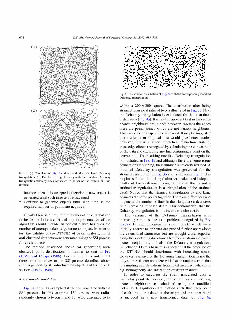
Fig. 3. (a) A set of anti-clustered circular data generated using the SSI

process described in the text. (b) The same set of data with a strain of

Rs ¼ 2.0.


intersect then it is accepted otherwise a new object is

generated until such time as it is accepted.

5. Continue to generate objects until such time as the

required number of points are acquired.

Clearly there is a limit to the number of objects that can

fit inside the finite area A and any implementation of the

algorithm should include an opt out clause based on the

number of attempts taken to generate an object. In order to

test the validity of the DTNNM of strain analysis, initial

anti-clustered data sets were generated using the SSI process

for circle objects.

The method described above for generating anti-

clustered point distributions is similar to that of Fry

(1979) and Crespi (1986). Furthermore it is noted that

there are alternatives to the SSI process described above

such as generating 3D anti-clustered objects and taking a 2D

section (Erslev, 1988).

4.3. Example simulation

Fig. 3a shows an example distribution generated with the

SSI process. In this example 160 circles, with radius

randomly chosen between 5 and 10, were generated to fit

within a 200 £ 200 square. The distribution after being

strained to an axial ratio of two is illustrated in Fig. 3b. Next

the Delaunay triangulation is calculated for the unstrained

distribution (Fig. 4a). It is readily apparent that in the centre

nearest neighbours are joined; however, towards the edges

there are points joined which are not nearest neighbours.

This is due to the shape of the area used. It may be suggested

that a circular or elliptical area would give better results;

however, this is a rather impractical restriction. Instead,

these edge effects are negated by calculating the convex hull

of the data and excluding any line containing a point on the

convex hull. The resulting modified Delaunay triangulation

is illustrated in Fig. 4b and although there are some rogue

connections remaining, their number is severely reduced. A

modified Delaunay triangulation was generated for the

strained distribution in Fig. 3b and is shown in Fig. 5. It is

emphasised that this triangulation was calculated indepen-

dently of the unstrained triangulation (i.e. this is not a

strained triangulation, it is a triangulation of the strained

data). Notice that the strained triangulation by and large

connects the same points together. There are differences and

in general the number of lines in the triangulation decreases

with increasing imposed strain. This demonstrates that the

Delaunay triangulation is not invariant under strain.

The variance of the Delaunay triangulation with

increasing strain is due to a problem recognised by Fry

(1979). During homogeneous strain, points which were

initially nearest neighbours are pushed further apart along

the extensional strain axis but are brought closer together

along the shortening direction. Therefore as strain increases,

nearest neighbours, and also the Delaunay triangulation,

will change. On this basis it is expected that the precision of

the DTNNM should deteriorate with increasing strain.

However, variance of the Delaunay triangulation is not the

only source of error and there will also be random errors due

to sampling and deviations from ideal assumed behaviour,

e.g. homogeneity and interaction of strain markers.

In order to calculate the strain associated with a

particular point distribution, the set of lines connecting

nearest neighbours as calculated using the modified

Delaunay triangulation are plotted such that each point

of each line is translated to the origin and the other point

is included in a new transformed data set. Fig. 6a

Fig. 4. (a) The data of Fig. 3a along with the calculated Delaunay

triangulation. (b) The data of Fig 3b along with the modified Delaunay

triangulation whereby lines connected to points on the convex hull are

omitted.

Fig. 5. The strained distribution of Fig. 3b with the corresponding modified

Delaunay triangulation.


illustrates this plot for the unstrained data and it clearly

exhibits a circular pattern. In Fig. 6b the data is

normalised according to Erslev (1988) and the central

void is very evidently a circle, as expected. Plots for the

strained data are shown in Fig. 7. The raw data is shown

in Fig. 7a and the normalised data are shown Fig. 7b.

Fig. 6. (a) Plot of the data from a modified Delaunay triangulation

corresponding to the unstrained example in Fig. 4b. (b) The same data after

normalisation.

Fig. 7. (a) Plot of the data from a modified Delaunay triangulation

corresponding to the strained example in Fig. 5. (b) The same data after

normalisation. (c) The same data after enhancement with sf ¼ 1.1.


However, the best result is obtained by applying the

enhancement suggest by Erslev and Ge (1990) whereby

only objects in close proximity are chosen for analysis.

The enhanced normalised plot is shown in Fig. 7c for a

selection factor of 1.1 and the data closely follow an

ellipse with axial ratio of two, i.e. the strain ellipse.

4.4. Results

Because a large volume of data was generated by the

simulation study, it is impractical to report it in a detailed

graphical format. Therefore the average error in Rscalc and

fscalc was calculated for n, sf and Rsact, where the average

Fig. 8. (a) Variation of average error (Rserr and fserr) with n. (b) Variation of average error (Rserr and fserr) with increasing selection factor, sf. (c) Variation of

average error (Rserr and fserr) with increasing imposed strain (Rsact).


Fig. 9. The percentage ratio of the number of data after processing (Nproc) to the number of data from the modified Delaunay triangulation (Ndel) as a function of

both sf and imposed strain (Rsact).

Fig. 10. Representative detailed results from the simulation study, showing Rsact/Rscalc versus sf along with confidence intervals for: (a) Rsact ¼ 2.0, Nobj ¼ 175,

(b) Rsact ¼ 5.8, Nobj ¼ 175, (c) Rsact ¼ 2.0, Nobj ¼ 330, and (d) Rsact ¼ 5.8, Nobj ¼ 330.


errors are calculated as:

Rserr ¼ 100Rscalcu 2 Rscalclj j

2Rscalc

ð11Þ

fserr ¼ 100fscalcu 2 fscalclj j

2ð12Þ

where Rserr is in percent and fserr is in degrees. From Fig. 8a

it is clear that as n increases the error tends to decrease. Note

that the number of objects analysed must be taken in the

context of the size of the area analysed in so far as 1000

loosely packed objects measured from a large area may not

be as effective as 200 closely packed objects from a smaller

region. A packing density, defined as the ratio of object area

to sample area, in conjunction with n may give a better

indication of the numbers of objects required to achieve a

desired level of accuracy. In the present simulation the

packing densities are 34, 39, 46, 49, 52 and 54.5%

corresponding to n ¼ 175, 205, 240, 270, 295 and 330,

respectively.

Increasing the selection factor tends to produce greater

errors in Rscalc and although an upward trend in the error for

fscalc may also be distinguished, it is not as pronounced (see

Fig. 8b). This indicates that for the most accurate results, the

value of sf should be chosen close to one. As the tectonic

strain increases (Rsact) the error associated with Rscalc

Fig. 11. Model of oolite data along with the corresponding modified

Delaunay triangulation.

Fig. 12. Results of analysis for various values of sf.


increases correspondingly, e.g. from 1% (Rsact < 1.2) up to

10% (Rsact < 5.8) (see Fig. 8c). This is due in part to the

variance of Delaunay triangulation (the changing nearest

neighbour problem identified by Fry (1979)); however, it

also incorporates statistical errors. This level of error is not

unexpected because methods based on strain marker shape

display errors of a comparable magnitude (Mulchrone and

Meere, 2001; Mulchrone et al., 2002). On the basis of error

characteristics alone, the DTNNM method (and presumably

other Fry methods) out perform both the method of Robin

(1977) and Mulchrone et al. (2002) using 100 strain markers

at strain ratios less than approximately 5.8 because these

methods are subject to a percentage error of approximately

13% for all strain ratios. By contrast with the error

behaviour of strain ratio estimation, the error in estimating

the orientation of the strain ellipse decreases rapidly as Rsact

increases (Fig. 8c).

In Fig. 9 the percentage ratio of the number of data after

enhancement (Nproc) to average number of data selected by

the modified Delaunay triangulation (Ndel) is compared with

sf for Rsact ¼ 1, 2, 3, 4 and 5. It is clear that as sf increases so

too does the percentage of data available for analysis. In

addition, as the imposed strain (Rsact) increases, the

percentage of data available for analysis decreases.

These results suggest that as sf increases the additional

data available for analysis tends to increase the error.

However, at higher imposed strain less data is selected but

the error is higher probably due to increased variability in

the selected data. In summary, this simulation study

suggests that the method proposed here is best suited to

low to moderate strains and that the most accurate results

are obtained by selecting low sf values.

Finally, representative detailed results are presented on

Rsact/Rscalc versus sf plots (similar to those of Borradaile

Fig. 13. (a) Variation of Rscalc, with confidence intervals, for sf ¼ 1.01 to 2. (b) Error variation with sf. Note that maximum Rscalc broadly corresponds to the

minimum in error.


(1986); see Fig. 10). Values of one for Rsact/Rscalc indicates

that the calculated strain matches the imposed strain exactly.

Confidence intervals are also divided by Rsact and so

represent percentage confidence intervals. These plots

mirror the general trends outlined above. For Nobj ¼ 175

(packing density of 34%), percentage confidence intervals

are larger than those for Nobj ¼ 330 (packing density of

54.5%) and in both cases the confidence intervals are much

larger for higher imposed strain values, i.e. Rsact ¼ 2.0 as

compared with 5.8. However, in almost every case (except

for the worst possible case of Nobj ¼ 175 and Rsact ¼ 5.8)

the calculated strain is within 10% of the true value and the

confidence intervals nearly always include Rsact/Rscalc ¼ 1.

This simulation study strongly suggests that the method

proposed here is valid and produces accurate results to a

95% level of confidence.

5. Application to real data

In order to demonstrate the applicability of the technique

described here and also to investigate its properties with real

data, the deformed ironstone oolite illustrated in fig. 7.7 of

Ramsay and Huber (1983, p. 112) was analysed. The raw

data parameters (ai, bi, xi, yi, fi ) were calculated and the

results of this are graphically illustrated in Fig. 11, along

with the modified Delaunay triangulation. It is clear that

nearest neighbours are connected in most cases. Plots of the

data resulting from the analysis are illustrated in Fig. 12 for

sf ¼ 1.01, 1.07, 1.22 and 1.3. In each case a clearly defined

ellipse is present. However, in order to decide which value

of sf gives the best estimate of the strain ellipse the errors

were studied in detail by varying sf in 0.01 steps.

By contrast with the simulation study above, analysis of

Fig. 14. (a) Variation of fscalc, with confidence intervals, for sf ¼ 1.01 to 2. (b) Error variation with sf. Note that maximum error in fscalc corresponds to the

minimum error in Rscalc (Fig. 13b).


natural data shows a systematic variation with sf (see Figs.

13 and 14). In Fig. 13a, Rscalc increases to a maximum at

sf < 1.3 and then falls off for higher values of sf. According

to the simulation study, the best estimate should be obtained

by choosing a low value for sf; however, in Fig. 13b, a

systematic variation in the error is also observed which

corresponds to the variation in Rscalc. Errors are much higher

for low and high sf but are at a minimum for 1.1 , sf , 1.3.

Furthermore, a similar pattern is observed for fscalc (see Fig.

14a and b), although the value of fscalc is not as variable as

Rscalc, and the minimum error is much more clearly defined.

Based on this data it is suggested that the best fit strain

ellipse may be estimated by choosing the value of sf that

minimises the errors, that is sf ¼ 1.22. The calculated strain

values are therefore given by Rscalc ¼ 1.69 ^ 0.01 and

fscalc ¼ 224.2 ^ 1.28. The approach of error minimisation

is not subjective and is a solution to the problem of how to

select an appropriate value for the selection factor

(McNaught, 1994). Furthermore, it is noted that Erslev

and Ge (1990) report strain estimates for this sample that are

somewhat lower (i.e. 1.598 up to 1.672); however, they used

sf ¼ 1.01 and 1.07 and had not minimised the errors.

It is interesting to note the differences between the

behaviour of error in the natural example and the simulated

data (see Fig. 8b). This is probably because the natural data

is not perfectly anti-clustered and the ooliths were not

originally perfectly circular.

As a cross check on the above results, the shapes of the

ooliths were analysed using the methods of Robin (1977)

and Mulchrone et al. (2002). The method of Robin (1977)

gives Rscalc ¼ 1.68 ^ 0.05 and fscalc ¼ 223.5 ^ 1.08,

whereas the mean radial length approach of Mulchrone

et al. (2002) gives Rscalc ¼ 1.69 ^ 0.05 and

fscalc ¼ 223.6 ^ 1.18. The strain ellipse calculated from

the nearest neighbour analysis and the methods based on the

shape of the ooliths are identical within the precision of

the methods. This result is somewhat surprising because the

oolite analysed has undergone significant oolith-scale

heterogeneous deformation by pressure solution. The

nearest neighbour method measures strain due to matrix

deformation and pressure solution; however, the methods

based on oolith shape assume that the ooliths deformed

passively and homogeneously along with the matrix. This is

clearly untrue. However, it appears that the pressure

solution component of deformation has modified oolith

shapes, such that they give an identical estimate of strain.

This raises an interesting (and unanswered) question

regarding the generality of this observation.

6. Conclusions

A method for objectively determining nearest neigh-

bours, namely the Delaunay triangulation, is introduced in

this paper. It is suggested that this approach makes the NNM

of strain analysis a practical (and computationally more

efficient) alternative to the Fry and associated methods.

Once nearest neighbours are selected, centre–centre

distances can be processed by normalisation (Erslev,

1988) and enhancement (Erslev and Ge, 1990). The best

fit ellipse is determined using a steepest gradient non-linear

least squares algorithm applied to the polar equation on a

centred ellipse. A simulation study indicates that the

technique is a valid one and estimates the strain ellipse

well at the 95% confidence interval. Application to a set of

natural oolite data shows that there is a systematic variation

of error with selection factor and it is suggested that the best

estimate of the strain ellipse is obtained by choosing the

selection factor which minimises the error. Moreover, the

estimates of strain calculated with the DTNNM are

comparable with estimates obtained using established

methods.

Acknowledgments

Thanks to Dr P.A. Meere, Department of Geology and

Prof. Y. Pawitan, Department of Statistics, UCC, for

reviewing an earlier version of this paper. The final version

of this paper has been greatly improved by the fair, critical

and thorough reviews of Drs E. Erslev and N. Fry.

References

Abell, M.L., Braselton, J.P., Rafter, J.A., 1999. Statistics with Mathema-

tica, Academic Press, San Diego.

Ailleres, L., Champenois, M., 1994. Refinements to the Fry method (1979)

using image processing. Journal of Structural Geology 16, 1327–1330.

Ailleres, L., Champenois, M., Macaudiere, J., Bertrand, J.M., 1995. Use of

image analysis in the measurement of finite strain by the normalized Fry

method: geological implications for the ‘Zone Houillere’ (Brianconnais

zone, French Alps). Mineralogical Magazine 59, 179–187.

Borradaile, G.J., 1986. Analysis of strained sedimentary fabrics: review and

test. Canadian Journal of Earth Science 24, 442–455.

Crespi, J.M., 1986. Some guidelines for the practical application of Fry’s

method of strain analysis. Journal of Structural Geology 8, 799–808.

Diggle, P.J., 1983. Statistical Analysis of Spatial Point Patterns, Academic

Press, London.

Draper, N.R., Smith, H., 1998. Applied Regression Analysis, John Wiley

and Sons, New York.

Edelsbrunner, H., 1987. Algorithms in Combinatorial Geometry, Springer-

Verlag, Berlin.

Erslev, E.A., 1988. Normalized centre-to-centre strain analysis of packed

aggregates. Journal of Structural Geology 10, 201–209.

Erslev, E.A., Ge, H., 1990. Least squares centre-to-centre and mean object

ellipse fabric analysis. Journal of Structural Geology 8, 1047–1059.

Fry, N., 1979. Random point distributions and strain measurement in rocks.

Tectonophysics 60, 806–807.

Hart, D., Rudman, A.J., 1997. Least-squares fit of an ellipse to anisotropic

polar data: application to azimuthal resistivity surveys in karst regions.

Computers and Geosciences 23, 189–194.

Huang, C.-W., Shih, T.-Y., 1998. Improvements on Sloan’s algorithm for

constructing Delaunay triangulations. Computer and Geosciences 24,

193–196.

McNaught, M., 1994. Modifying the normalized Fry method for aggregates

of non-elliptical grains. Journal of Structural Geology 16, 493–503.


Mulchrone, K.F., 2001. Quantitative estimation of exponents of power-law

flow with confidence intervals in ductile shear zones. Journal of

Structural Geology 23, 803–806.

Mulchrone, K.F., Meere, P.A., 2001. A windows program for the analysis

of tectonic strain using deformed elliptical markers. Computers and

Geosciences 27, 1253–1257.

Mulchrone, K.F., O’Sullivan, F., Meere, P.A., 2002. Finite strain estimation

using the mean radial length of elliptical objects with confidence

intervals. Journal of Structural Geology in press PII: S0191-

8141(02)00049-4.

O’ Rourke, J., 1993. Computational Geometry in C, Cambridge University

Press, Cambridge.

Perparata, F.P., Shamos, M.I., 1985. Computational Geometry: an

Introduction, Springer-Verlag, New York.

Ramsay, J.G., 1967. Folding and Fracturing of Rocks, McGraw-Hill, New

York.

Ramsay, J.G., Huber, M.I., 1983. The Techniques of Modern Structural

Geology, Volume 1: Strain Analysis, Academic Press, London.

Robin, P.F., 1977. Determination of geologic strain using randomly

oriented strain markers of any shape. Tectonophysics 42, T7–T16.


Application of Delaunay triangulation to the nearest neighbour method of strain analysis

Documents

Transcript of Application of Delaunay triangulation to the nearest neighbour method of strain analysis