A comparison of k-nearest neighbour algorithms with performance results on speech data

A comparison of k-nearest neighbour

algorithms with performance results on

speech data

Mike Matton and Ronald Cools

Report TW381, January 2004

Katholieke Universiteit LeuvenDepartment of Computer Science

Celestijnenlaan 200A – B-3001 Heverlee (Belgium)

A comparison of k-nearest neighbour

algorithms with performance results on

speech data

Mike Matton and Ronald Cools

Report TW381, January 2004

Department of Computer Science, K.U.Leuven

Abstract

The (k-)nearest neighbour problem is well known in a wide rangeof areas. Many algorithms to tackle this problem suffer from the“curse of dimensionality” which means that the execution time growsexponentially with increasing dimension. Therefore, it is importantto have efficient algorithms for the problem.

In this report, some well known tree-based algorithms for thek-nearest neighbour are investigated and tested on speech data. Weexperimentally derive the time complexity as a function of the num-ber of nearest neighbours k, the database size n and the bucketsize b.

Keywords : nearest neighbours search complexity approximate kd-tree bbd-tree

Contents

1 Introduction 1

2 Basics 1

2.1 Tree Structures . . . . . . . . . . . . . . . . . . . . . . . . . . . . . . . . . . . 12.1.1 Kd-trees . . . . . . . . . . . . . . . . . . . . . . . . . . . . . . . . . . . 22.1.2 Bbd-trees . . . . . . . . . . . . . . . . . . . . . . . . . . . . . . . . . . 3

2.2 Search Algorithms . . . . . . . . . . . . . . . . . . . . . . . . . . . . . . . . . 42.2.1 The Standard Kd-tree Search . . . . . . . . . . . . . . . . . . . . . . . 42.2.2 Priority Search . . . . . . . . . . . . . . . . . . . . . . . . . . . . . . . 4

3 Experiments 5

3.1 Exact vs Approximate k-nearest neighbours . . . . . . . . . . . . . . . . . . . 63.2 The Bucket Size . . . . . . . . . . . . . . . . . . . . . . . . . . . . . . . . . . 63.3 Scale-up . . . . . . . . . . . . . . . . . . . . . . . . . . . . . . . . . . . . . . . 73.4 Kd-trees vs Bbd-trees and k-nearest neighbours . . . . . . . . . . . . . . . . . 73.5 Standard vs Priority Search . . . . . . . . . . . . . . . . . . . . . . . . . . . . 83.6 Splitting Rules and the Cell Aspect Ratio . . . . . . . . . . . . . . . . . . . . 93.7 Empirical complexity of the search . . . . . . . . . . . . . . . . . . . . . . . . 9

3.7.1 Time complexity in the number of datapoints . . . . . . . . . . . . . . 93.7.2 Time complexity in the number of requested nearest neighbours . . . 9

4 Future Work 11

5 Conclusion 12

i

1 Introduction

The (k-) nearest neighbour problem occurs in a wide range of areas, including pattern recog-nition, speech and image processing, data compression, databases, computer graphics etc . . . .In many cases this problem has to be tackled in high-dimensional spaces (ranging from two toa few hundred of dimensions). However, the amount of computing time necessary to solve theproblem grows exponentially with increasing dimension. Therefore, high-performance searchstructures and algorithms have to be developed to reduce the necessary computation time.Two such search structures are kd-trees [5] and bbd-trees [2], which are compared in thisreport.

2 Basics

The Curse of Dimensionality Many (if not all) k-nearest neighbour algorithms sufferfrom the curse of dimensionality [4]. In terms of the k-nearest neighbour problem, the cursemeans that the number of data points that has to be investigated increases exponentiallywith the dimension of these points. One possible explanation for this is that the variances ofthe distances of uniform data decrease with increasing dimension (this means that the moredimensions you have, the closer the nearest and the farthest neighbour are to each other).

Exact vs Approximate Nearest Neighbours Several researchers have tried to reducethe complexity of the nearest neighbour search by relaxing the query. Instead of finding theexact k-nearest neighbours, the ε-k-nearest neighbours suffice. A point p is an ε-k’th nearestneighbour of a query point q if the ratio of the distances between p and q and between thereal k’th nearest neighbour and q is not larger than 1 + ε. The first researcher who usedthis idea was Arya [3]. Later, several others proposed algorithms for the approximate nearestneighbour problem.

2.1 Tree Structures

Many practical k-nearest neighbour search algorithms use tree structures to index the data.Among those structures are Samet’s quad-trees [15], kd-trees originally proposed by Bentley[5] with its different variants [9, 14] and bbd-trees proposed by Arya [2]. Good overviews ofdifferent indexing structures based on trees are written by Gaede et al. [10] and Bohm et al.[6].

There are a lot of tree structures described in the literature. Many of them use hyperplanesto split the data. In this section, two kinds of these trees, those that were used in theexperiments, are explained, namely kd-trees and bbd-trees. A short overview is given on howsuch a tree is created and the complexity of tree creation is mentioned. But first, the distancemeasures between two points that are used by these tree algorithms are explained.

Distance measures.

Friedman uses the notion of a dissimilarity measure D(x,y) to capture the “distance”between two points x,y ∈ R

d. He defines a dissimilarity measure as:

1

D(x,y) = F (k

∑

i=1

fi(xi, yi)). (1)

where fi is the coordinate distance along coordinate i. F and fi have to satisfy the followingproperties:

1. symmetryfi(x, y) = fi(y, x), i = 1, . . . , d (2)

2. monotonicityF (x) ≥ F (y) if x > y (3)

fi(x, z) ≥ fi(x, y) if z ≥ y ≥ x or x ≥ y ≥ z, i = 1, . . . , d (4)

When constructing a kd-tree, one can use a variety of distance measures. In theory, everymeasure that satisfies the symmetry (2) and monotonicity properties (3) (4) can be used toconstruct a kd-tree. The triangle inequality is not strictly needed. However, it is importantthat the distance function can be split along the coordinates because the kd-tree algorithmsalso uses “partial distances” along some of the coordinates. One of the most used set ofdistance measures is the set of vector space p-norms, also called Minkowski metrics, definedas

Dp(x,y) =

[

k∑

i=1

|xi − yi|p

]1/p

. (5)

Specific well known instances of this formula are the Euclidean distance (p = 2), the maximumdistance (p = ∞) and the Manhattan distance (p = 1). In the experiments described in thisreport, the Euclidean distance is used.

2.1.1 Kd-trees

Kd-trees were invented by Bentley [5] and proposed as a tool for fast nearest neighbourqueries. At each node of the tree, the data space is split with a hyperplane along one ofthe basic dimensions. Originally, as proposed by Bentley, the space is split along consecutivedimensions of the search space at each level of the tree. So, in the root node, the space is splitalong the first dimension, on the second level, the split occurs along the second dimensionetc . . . . A few years later, Friedman proposed, together with Bentley, another way to choosethe splitting direction. He used the direction with the maximal variance of point coordinates[9]. An example of a point cloud with its space partitioning and the corresponding kd-tree isshown in fig. 1.

Another parameter in kd-trees is the so called “bucket size”. This is the maximal numberof data points that can be put in a leaf node of the kd-tree. The standard tree as proposed byBentley uses a bucket size of 1, but there are valid arguments to increase this bucket size. Oneof the arguments is that elements that are in the same bucket have a high probability to beclose to each other, so if one of the points in the bucket is a k-nearest neighbour, some of theother points in the bucket are it probably too. In this case, the standard kd-tree algorithmwith bucket size 1 will probably cause more overhead than the computation of the distancefrom the query point to all the points in the bucket.

2

One of the disadvantages of the kd-tree is that buckets can become very narrow. Theresult of this is that, when searching for nearest neighbours, more nodes have to be examined,increasing the computing time. To overcome this, another criterion called “balanced aspectratio” was introduced. However, for certain data distributions, the kd-tree algorithm fails tomeet this criterion [8]. On the other hand, the splitting in kd-trees occurs along the medianof the coordinate values in the split direction. It is easy to see that in this case, the balancedaspect ratio is not always guaranteed. To overcome this, some alternative splitting rules havebeen proposed.

��

��

��

��

��

�

��

��

��

��

��

��

��

��

4

7

51

2

3

6

10

8

911

21

3

4 5

6

7 8

9 10 11

Figure 1: Point cloud and its corresponding kd-tree

Alternatives for the splitting rule. As mentioned above, the standard kd-tree algorithmuses a median splitting rule. It is easy to see that, for certain non-uniform data distributions,this leads to splits which violate the balanced aspect ratio criterion. Most alternative splittingrules guarantee the balanced aspect ratio, but to do this, they don’t provide an equal distri-bution of the data over the tree any more. This leads to unbalanced trees. Some performanceresults on these splitting rules are shown in section 3.6 on p. 9.

Time complexity The expected time complexity of kd-tree construction is

O(dN log N) (6)

with d the dimension of the search space and N the number of data points. This is not thatimportant because the tree creation has to occur only once. The complexity of the searchalgorithm is much more important.

2.1.2 Bbd-trees

Bbd-trees (balanced box decomposition) were introduced by Arya [2]. This type of treesuses two splitting criteria in the tree nodes. The first one is an iso-oriented hyperplane, similarto the ones used in kd-trees. The second one is a shrink operation which zooms in on thedata (if the data is highly clustered). For this shrink-operation, different alternatives havebeen proposed by Ayra, details can be found in [2].

3

Another aspect of these trees is that they satisfy the “balanced aspect ratio” criterion. Aconsequence of this is that bbd-trees cannot guarantee that the points are evenly distributedand the resulting tree may not be balanced.

Time complexity The expected time complexity for bbd-tree time construction is equalto that of kd-tree construction, namely O(dN log N).

2.2 Search Algorithms

2.2.1 The Standard Kd-tree Search

An algorithm for searching the k nearest neighbours of a query point using optimized kd-trees was proposed by Friedman [9]. Summarized, this algorithm searches the kd-tree, startingwith the node in which the query point is located until the hypersphere centered at the querypoint and with radius the distance to the k’th closest nearest neighbour found so far, fitsentirely within the kd-node currently under investigation. In this case, all remaining pointsin the kd-tree are further away than that k’th closest nearest neighbour so these points don’tneed to be investigated.

Figure 2 shows an example of a kd-tree search for one nearest neighbour. The square-shapedpoint is the query point for which the nearest neighbour has to be found. The * indicates thecurrently investigated node and the highlighted point is the current point marked as nearestneighbour.

Complexity The complexity of the kd-tree search algorithm is not easily derivable. In hispaper, Friedman derives that the search time is logarithmic in file size [9]. He also statesthat the number of records that is examined for the k nearest neighbours according to the∞-distance in the ideal case is

R∞(k, d) = (k1/d + 1)d, (7)

which shows an exponential behaviour in the dimension (curse of dimensionality) and a sub-linear behaviour in the number of nearest neighbours. However, practical experiments showthat the real behaviour of the kd-tree search algorithm is much worse (even super-linear). Foran empirical derivation of the time complexity in the number of requested nearest neighbours,see section 3.7.2 on p. 9.

For the bbd-trees, Arya was not able to give bounds on the runtime other than a trivialone. His search algorithm also suffers from the curse of dimensionality: its complexity hasexponential factors in the dimension of the search space too.

2.2.2 Priority Search

Priority search is a search technique that lists the nodes in the search tree in a somewhatmore intelligent way compared to the standard kd-tree search. It visits the nodes in the treein order of increasing distance to the query point q. This technique is described by Arya andMount [3]. The technique can be implemented in an easy way using a priority queue. Ateach internal node in the search algorithm, the distance of the query point q to the farthest

4

(a)

��

��

��

��

��

�

��

��

��

��

��

��

��

��

��

��

��

!!!

(b)

""##

$$%%

&&''

(())

**++,,-

-

..//

0011

2233

4455

6677

88888888888888888888888888

9�9�9�9�9�9�9�9�9�9:�:�:�:�:�:�:�:�:�:

;�;�;�;�;�;�;�;�;�;<�<�<�<�<�<�<�<�<

=�=�=�=�=�=�=�=�=�=�=>�>�>�>�>�>�>�>�>�>

????????????????

@@@@@@@@@@@@@@@@

AAABBB

*

(c)

CCDD

EEFF

GGHH

IIJJ

KKLLMMN

N

OOPP

QQRR

SSTT

UUVV

WWXX

YYYYYYYYYYYYYYYYYYYYYYYYYY

ZZZZZZZZZZZZZZZZZZZZZZZZZZ

[[[[[[[[[[[[[[[[[[[[[[

\\\\\\\\\\\\\\\\\\\\\\

]�]�]�]�]�]�]�]�]�]�]^�^�^�^�^�^�^�^�^�^�^

_�_�_�_�_�_�_�_�_�_`�`�`�`�`�`�`�`�`�`

aaaaaaaaaaaa

b�b�b�b�b�b�b�b�b�b�bc�c�c�c�c�c�c�c�c�c�c

dddeee

*

(d)

ffgg

hhii

jjkk

llmm

nnooppq

q

rrss

ttuu

vvww

xxyy

zz{{

||||||||||||||||||||||||||

}�}�}�}�}�}�}�}�}�}~�~�~�~�~�~�~�~�~�~

��

��

��

*(e)

��

��

��

��

��

�

��

��

��

��

��

��

��

��

��

��

*

(f)

¡¡

¢¢££

¤¤¥¥

¦¦§§

¨¨©©ªª«

«

¬¬

®®¯¯

°°±±

²²³³

´´µµ

¶¶¶¶¶¶¶¶¶¶¶¶¶¶¶¶¶¶¶¶¶¶¶¶¶¶

··························

¸¸¸¸¸¸¸¸¸¸¸¸¸¸¸¸¸¸¸¸¸¸

¹�¹�¹�¹�¹�¹�¹�¹�¹�¹�¹º�º�º�º�º�º�º�º�º�º

»»»»»»»»»»»»

¼¼¼¼¼¼¼¼¼¼¼¼

½½¾¾

*

(g)

¿¿ÀÀ

ÁÁÂÂ

ÃÃÄÄ

ÅÅÆÆ

ÇÇÈÈÉÉÊ

Ê

ËËÌÌ

ÍÍÎÎ

ÏÏÐÐ

ÑÑÒÒ

ÓÓÔÔ

ÕÕÕÕÕÕÕÕÕÕÕÕÕÕÕÕÕÕÕÕÕÕÕÕÕ

ÖÖÖÖÖÖÖÖÖÖÖÖÖÖÖÖÖÖÖÖÖÖÖÖÖ

××××××××××××××××

ØØÙÙ

*

(h)

ÚÚÛÛ

ÜÜÝÝ

ÞÞßß

ààáá

ââããääå

å

ææçç

èèéé

êêëë

ììíí

îîïï

ððððððððððððððððððððððððð

ññññññññññññññññ

òòòòòòòòòòòòòòòò

óóôô

Figure 2: Kd-tree standard search algorithm

child node is inserted into the sorted priority queue. If the search arrives at a leaf node, thedistances to the points in that leaf node are computed and then, if necessary, the next elementin the priority queue is investigated by the search.

3 Experiments

To test the performance of these algorithms, the ANN (approximate nearest neighbours)toolbox of Arya [1] was used. The toolbox is used to compare kd-trees and bbd-trees, toexperiment with different bucket sizes, to examine exact and approximate nearest neighbours,to compare standard search and priority search and to perform scale-up experiments. Thedatabase consists of a set of 15 dimensional feature vectors obtained from the TiDigits dataset for speaker independent digit recognition [13].

5

3.1 Exact vs Approximate k-nearest neighbours

In a first experiment, it is checked in what way the introduction of the approximation factorε improves the performance of the search. The measurements are summarized in fig. 3. Itcan be seen from fig. 3b that the relative gain in computing time decreases with increasingnumber of requested nearest neighbours. Further experiments point out that with an ε factorof 1, about 75-85% of the real nearest neighbours are part of the computed approximatenearest neighbours. With ε = 2 this is about 50%. Details are given in table 1.

1000 2000 3000 4000 5000 6000 7000 8000 9000 100000

0.2

0.4

0.6

0.8

1

1.2

1.4

Number of nearest neighbours

Mea

n ex

ecut

ion

time

per

quer

y

eps=0eps=0.5eps=1

1000 2000 3000 4000 5000 6000 7000 8000 9000 100000

0.2

0.4

0.6

0.8

1


norm

aliz

ed e

xecu

tion

time

(wrt

eps

=0)

Figure 3: (a) searching 1000-10000 (approximate) nearest neighbours with a K-D-Tree in a1516015 point TiDigits data set for varying ε. (b) same as (a) but with ε = 0 execution timesnormalized to 1.

ε 100-nn 1000-nn 5000-nn 10000-nn

0 100% 100% 100% 100%

1 85.36% 81.07% 77.66% 75.95%

2 54.88% 51.17% 49.50% 49.12%

Table 1: Number of exact k-nearest neighbours computed as function of ε.

3.2 The Bucket Size

For determining the optimal bucket size, mean execution time per query is computed as afunction of the bucket size. This relation is plotted in fig. 4 on p. 7. The behaviour shownin this figure will be typical for most databases. First, as the bucket size increases, the meanexecution time will drop. The search algorithm will produce too much overhead when thebucket size is too low. At a certain point the curve will reach a minimum after which itwill start to increase again because then the problem will converge to a brute force search(when the bucket size is bigger than the database size). The location of this minimum couldbe different for different problems. For this database, the optimal bucket size for computing10000 nearest neighbours is around 20.

6

100

101

102

103

0.75

0.8

0.85

0.9

0.95

1

1.05

1.1

1.15

Bucket size

Mea

n ex

ecut

ion

time

per

quer

y

Figure 4: Query execution time as a function of the bucket size

3.3 Scale-up

In this experiment, some scale-up experiments were performed on the data set using kd-trees. According to Friedman, the complexity of the search should be logarithmic in file sizeN [9]. The measurements with the ANN toolbox are shown in fig. 5. The main problemwith k nearest neighbours algorithms is the exponential factor in the dimension of the searchspace, which is a very large constant factor.

1000 2000 3000 4000 5000 6000 7000 8000 9000 100000

0.5

1

1.5


mea

n ex

ecut

ion

time

per

quer

y (s

ecs)

n=100000n=300000n=500000n=1000000n=1500000

0 5 10 15

x 105

0.7

0.8

0.9

1

1.1

1.2

1.3

1.4

1.5

Number of points in db

mea

n ex

ecut

ion

time

per

quer

y (s

ecs)

Figure 5: Scale-up experiment with kd-trees. (a) results for various file sizes and number ofnearest neighbours. (b) results for 10000 nearest neighbours and varying file size

3.4 Kd-trees vs Bbd-trees and k-nearest neighbours

Fig. 6 shows a comparison between kd-trees and bbd-trees for the approximate nearestneighbours problem with ε = 1. Strangely, the performance of the bbd-tree search is worsethan the performance of the kd-tree search. A possible explanation for this is that the data

7

is not highly clustered and in that case the bbd-algorithm only produces overhead becausethe shrink operation will seldomly be used.

1000 2000 3000 4000 5000 6000 7000 8000 9000 100000

0.2

0.4

0.6

0.8

1

1.2

1.4


Mea

n ex

ecut

ion

time

per

quer

y (s

ecs)

ANN Toolbox − − n=1516015 d=15 eps=1 (archimedes)

kd−treebbd−tree

Figure 6: comparison searching 1000-10000 approximate nearest neighbours with kd-tree -bbd-tree in a 1516015 point TiDigits data set

3.5 Standard vs Priority Search

Another experiment compares the standard kd-search algorithm (section 2.2.1) and thepriority search algorithm (section 2.2.2). The results of this comparison are displayed in fig.7. As can be seen, the introduction of the priority search technique improves the performanceof the search drastically for kd-trees as for bbd-trees. The behaviour it now shows is almostlinear (only a slight curve) for the first 10000 nearest neighbours. As fig. 7.c shows, theexecution time of the search is quadratic in the number of nearest neighbours.

1000 2000 3000 4000 5000 6000 7000 8000 9000 100000

0.2

0.4

0.6

0.8

1

1.2

1.4


mea

n ex

ecut

ion

time

per

quer

y

kd−tree normal searchkd−tree priority searchbd−tree normal searchbd−tree priority search

1000 2000 3000 4000 5000 6000 7000 8000 9000 100000.2

0.3

0.4

0.5

0.6

0.7

0.8

0.9

1

1.1

Number of requested nearest neighbours

Mea

n qu

ery

exec

utio

n tim

e

Figure 7: Comparison between standard kd-tree search and priority search (a) real executiontimes. (b) execution times for kd-tree normal search is normalized to 1.

8

3.6 Splitting Rules and the Cell Aspect Ratio

Experiments with the standard kd-tree split rule have shown that the mean aspect ratio ofthe cells is quite large (over 33). The aspect ratio is the ratio between the lengths of thelongest and the shortest boundaries of the cell. If this ratio is large this means that the cellis quite “skinny”. One can intuitively see that this degrades performance of the search. Inthis experiment another splitting rule is chosen (sliding midpoint splitting) which guaranteesa lower aspect ratio. Some results are shown in fig. 8. The restriction of balanced aspect ratioprovides only minor improvements to the search performance.

1000 2000 3000 4000 5000 6000 7000 8000 9000 100000

0.2

0.4

0.6

0.8

1

1.2

1.4

1.6

Mea

n ex

ecut

ion

time

per

quer

y


Figure 8: comparison splitting rules. blue = standard split, red = sliding midpoint split

3.7 Empirical complexity of the search

3.7.1 Time complexity in the number of datapoints

According to Friedman, the time complexity of the k nearest neighbour search with kd-treesis O(log n). This can be empirically verified by producing a logplot of the execution times ofthe scale-up experiment from section 3.3. If the complexity is indeed logarithmic, this plotshould appear as a straight line. Such a logplot is shown in fig. 9 on p. 10. As expected, thisplot indeed is approximately straight.

3.7.2 Time complexity in the number of requested nearest neighbours

The derivation of the time complexity as a function of the number of requested nearestneighbours is more difficult. Friedman, nor any researcher after him was able to give a timecomplexity as a function of the number of requested nearest neighbours. For ideal cases andthe maximum distance, the complexity could be approximated using eq. 7 on p. 4. Accordingto this equation, the time complexity should be sublinear in k. In practice this is not the caseas can be derived from several plots in this report. Intuitively (from the plots) one wouldexpect this complexity to be O(k2) or O(k log k).

9

0 5 10 15

x 105

0.7

0.8

0.9

1

1.1

1.2

1.3

1.4

1.5

Mea

n ex

ecut

ion

time

per

quer

y

Number of points in database10

510

610

70.7

0.8

0.9

1

1.1

1.2

1.3

1.4

1.5

Mea

n ex

ecut

ion

time

per

quer

y

Number of points in database

Figure 9: (a) mean execution time as function of number of requested nearest neighbours.(b) logplot of (a)

If the complexity is O(k log k) then a logplot of the function t(k)/k should be a straightline for k large enough. Such a plot is shown in fig. 10 on p. 10. This is not at all a straightline, rejecting the hypothesis that the complexity is O(k log k).

0 0.2 0.4 0.6 0.8 1 1.2 1.4 1.6 1.8 2

x 104

0

0.5

1

1.5

2

2.5

3

3.5

4

4.5

5

Number of requested nearest neighbours

Mea

n ex

ecut

ion

time

per

quer

y

103

104

105

0.8

1

1.2

1.4

1.6

1.8

2

2.2

2.4x 10

−4

Number of requested nearest neighbours (k)

(Mea

n ex

ecut

ion

time

per

quer

y) /

k

Figure 10: (a) Mean execution times for increasing k (b) Logplot showing k on the x-axis andt(k)/k on the y-axis

Another possibility is that the complexity is polynomial in k, most probably quadratic.To check this, several polynomials of increasing order are estimated using the least squarescriterion. The variance of the error is a good statistic to determine the optimal degree of thepolynomial. The error variance for polynomials of increasing degree is shown in table 2 onp. 11, the polynomials in this table were made monic (a part from the sign of the highestorder coefficient). From degree 2 on, this variance is small and it is smallest for a degree of 3.However, a closer look at the coefficients of the third order polynomial shows a highest ordercoefficient that is negative. This is very unlikely and therefore the second order approximationis preferred. This would mean that the time complexity in k is indeed quadratic and thereis even more evidence for this: if we look at the plot of t(k)/k on a standard scale shown in

10

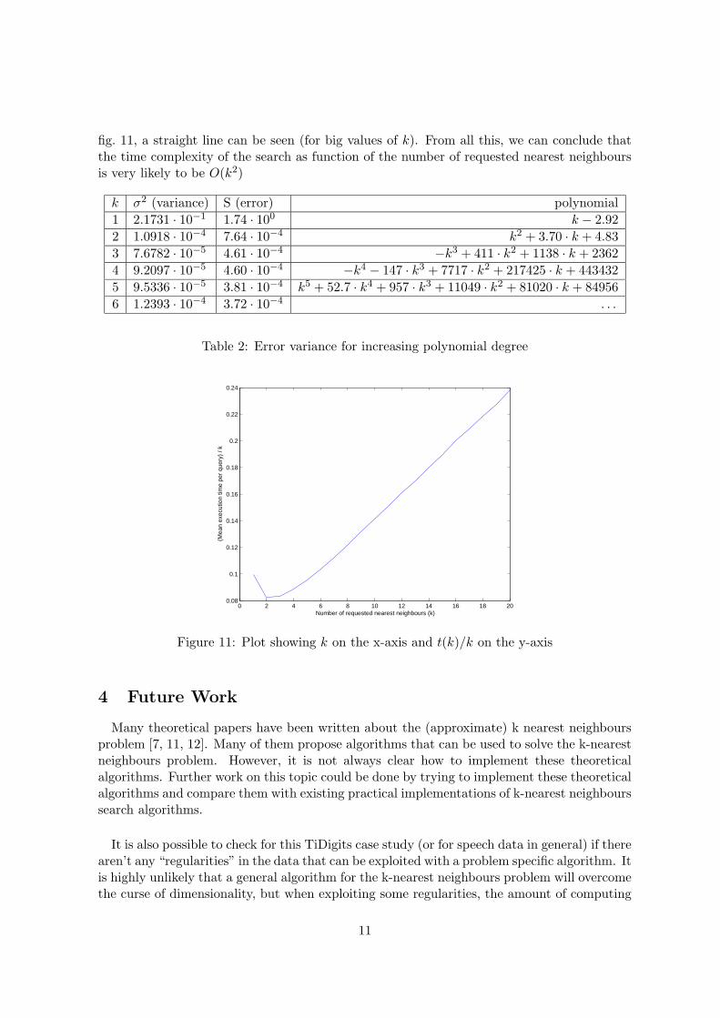
fig. 11, a straight line can be seen (for big values of k). From all this, we can conclude thatthe time complexity of the search as function of the number of requested nearest neighboursis very likely to be O(k2)

k σ2 (variance) S (error) polynomial

1 2.1731 · 10−1 1.74 · 100 k − 2.92

2 1.0918 · 10−4 7.64 · 10−4 k2 + 3.70 · k + 4.83

3 7.6782 · 10−5 4.61 · 10−4 −k3 + 411 · k2 + 1138 · k + 2362

4 9.2097 · 10−5 4.60 · 10−4 −k4 − 147 · k3 + 7717 · k2 + 217425 · k + 443432

5 9.5336 · 10−5 3.81 · 10−4 k5 + 52.7 · k4 + 957 · k3 + 11049 · k2 + 81020 · k + 84956

6 1.2393 · 10−4 3.72 · 10−4 . . .

Table 2: Error variance for increasing polynomial degree

0 2 4 6 8 10 12 14 16 18 200.08

0.1

0.12

0.14

0.16

0.18

0.2

0.22

0.24

Number of requested nearest neighbours (k)

(Mea

n ex

ecut

ion

time

per

quer

y) /

k

Figure 11: Plot showing k on the x-axis and t(k)/k on the y-axis

4 Future Work

Many theoretical papers have been written about the (approximate) k nearest neighboursproblem [7, 11, 12]. Many of them propose algorithms that can be used to solve the k-nearestneighbours problem. However, it is not always clear how to implement these theoreticalalgorithms. Further work on this topic could be done by trying to implement these theoreticalalgorithms and compare them with existing practical implementations of k-nearest neighbourssearch algorithms.

It is also possible to check for this TiDigits case study (or for speech data in general) if therearen’t any “regularities” in the data that can be exploited with a problem specific algorithm. Itis highly unlikely that a general algorithm for the k-nearest neighbours problem will overcomethe curse of dimensionality, but when exploiting some regularities, the amount of computing

11

time needed could possibly be improved. However, it is not clear which regularities are easyexploitable and, more important, how they can be exploited. Some more work could be doneon trying to identify such regularities in the data set (speech data in this case) and designingsome ways to exploit these.

5 Conclusion

The k-nearest neighbour problem is a very time-consuming search problem and will prob-ably remain this for quite a while. The main problem with k-nearest neighbours in highdimensions is the so-called “curse of dimensionality” that causes constant factors exponen-tial in the dimension of the search space in the complexity of the search algorithms. Manyattempts have been made to overcome this exponential dependence but none have reallysucceeded until now and the question is if it will in the near future. Even a relaxation ofthe problem: ε-approximate nearest neighbours did not improve performance very much (theexponential factor is still there).

On the other hand, the introduction of priority search has a significant impact on theperformance of the search, at least for the database used in this case study. The cell aspectratio seems a less important feature when comparing performance statistics.

12

References

[1] S. Arya. Ann: Library for approximate nearest neighbor searching v0.2, 1998.

[2] S. Arya, D. M. Mount, N. S. Netanyahu, R. Silverman, and A. Y. Wu. An optimalalgorithm for approximate nearest neighbor searching in fixed dimensions. Journal of

the ACM, 45(6):891–923, November 1998.

[3] Arya, S. and Mount, David M. Approximate Nearest Neighbor Queries in Fixed Dimen-sions. In Proceedings of the 4th Annual ACM Symposium on Discrete Algorithms, pages271–280, Austin, January 1993.

[4] R. Bellman. Adaptive Control Processes. Princeton University Press, 1961.

[5] J.L. Bentley. Multidimensional binary search trees used for associative searching. Com-

munications of the ACM, 18(9):509–517, September 1975.

[6] C. Bohm, S. Berchtold, and D.A. Keim. Searching in high-dimensional spaces - indexstructures for improving the performance of multimedia databases. ACM Computing

Surveys, 33(3):322–373, September 2001.

[7] Timothy M. Chan. Approximate nearest neighbours revisited. Discrete and Computa-

tional Geometry, 20(3):359–373, October 1998.

[8] A. Christian Duncan, Michael T. Goodrich, and Stephen Kobourov. Balanced aspectratio trees: Combining the advantages of k-d trees and octrees. In Proceedings of the

10th Annual ACM-SIAM Symposium on Discrete Algorithms, pages 300–309, Baltimore,January 1999.

[9] J.H. Friedman, J.L. Bentley, and Finkel R.A. An algorithm for finding best matches inlogarithmic expected time. ACM Transactions on Mathematical Software, 3(3):209–226,September 1977.

[10] V. Gaede and O. Gunther. Multidimensional access methods. ACM Computing Surveys,30(2):170–231, June 1998.

[11] Piotr Indyk and Rajeev Motwani. Approximate nearest neighbors: towards removing thecurse of dimensionality. In Proceedings of the 30th Annual ACM Symposium on Theory

of Computing, pages 604–613, Dallas, May 1998.

[12] Jon M. Kleinberg. Two algorithms for nearest-neighbour search in high dimensions.In Proceedings of the 29th Annual ACM Symposium on Theory of Computing, pages599–608, El Paso, May 1997.

[13] Leonard, R. Gary. A Database for Speaker Independent Digit Recognition. In Proceedings

of the IEEE ICASSP’84, pages 328–331, San Diego, March 1984.

[14] James McNames. A fast nearest-neighbour algorithm based on a principal axis searchtree. IEEE Transactions on Pattern Analysis and Machine Intelligence, 23(9):964–976,September 2001.

[15] Hanan Samet. The quadtree and related hierarchical data structures. ACM Computing

Surveys, 16(2):187–260, June 1984.

A comparison of k-nearest neighbour algorithms with performance results on speech data

Documents

Transcript of A comparison of k-nearest neighbour algorithms with performance results on speech data