sensors

Article

RBFNN Design Based on Modified Nearest NeighborClustering Algorithm for Path Tracking Control

Dongxi Zheng 1,2, Wonsuk Jung 3,* and Sunghoon Kim 1,4,*

�����������������

Citation: Zheng, D.; Jung, W.; Kim, S.

RBFNN Design Based on Modified

Nearest Neighbor Clustering

Algorithm for Path Tracking Control.

Sensors 2021, 21, 8349. https://

doi.org/10.3390/s21248349

Received: 29 November 2021

Accepted: 12 December 2021

Published: 14 December 2021

Publisher’s Note: MDPI stays neutral

with regard to jurisdictional claims in

published maps and institutional affil-

iations.

Copyright: © 2021 by the authors.

Licensee MDPI, Basel, Switzerland.

This article is an open access article

distributed under the terms and

conditions of the Creative Commons

Attribution (CC BY) license (https://

creativecommons.org/licenses/by/

4.0/).

1 Department of Electronics Convergence Engineering, Wonkwang University, Iksan 54538, Korea;zhengdongxi1979@wku.ac.kr

2 School of Mechanical and Intelligent Manufacturing, Jiujiang University, Jiujiang 332005, China3 School of Mechanical Engineering, Chungnam National University, Daejeon 34134, Korea4 Wonkwang Institute of Material Science and Technology, Wonkwang University, Iksan 54538, Korea* Correspondence: wonsuk81@cnu.ac.kr (W.J.); kshoon@wku.ac.kr (S.K.); Tel.: +82-63-850-6739 (S.K.)

Abstract: Radial basis function neural networks are a widely used type of artificial neural network.The number and centers of basis functions directly affect the accuracy and speed of radial basis func-tion neural networks. Many studies use supervised learning algorithms to obtain these parameters,but this leads to more parameters that need to be determined, thereby making the system morecomplex. This study proposes a modified nearest neighbor-based clustering algorithm for trainingradial basis function neural networks. The calculation of this clustering algorithm is not large, and itcan adapt to varying densities. Furthermore, it does not require researchers to set parameters basedon experience. Simulation proves that the clustering algorithm can effectively cluster samples andoptimize the abnormal samples. The radial basis function neural network based on modified nearestneighbor-based clustering has higher accuracy in curve fitting than the conventional radial basisfunction neural network. Finally, the path tracking control based on a radial basis function neuralnetwork of a magnetic microrobot is investigated, and its effectiveness is verified through simulation.The test accuracy and training accuracy of the radial basis function neural network was improved by23.5% and 7.5%, respectively.

Keywords: radial basis function neural network (RBFNN); nearest neighbor-based clustering (MNNC);sample optimization; path tracking

1. Introduction

Path tracking control is a commonly used motion control method for vehicles androbots. Owing to its simple structure, easy operation and adjustment, and robustness, theproportion integral differential (PID, as shown in Appendix A) controller is often used forpath tracking control [1,2]. However, the ability of PID in dealing with nonlinear systemsis limited. Therefore, fuzzy PID control was developed. B.B. Ghosh et al. developed afuzzy-PID-based controller to control the two degrees of freedom parallel manipulator.The control system has almost no overshoot based on the fuzzy-PID [3]. J.A. Algarin-Pintoet al. compared the fuzzy-PID with general PID for path tracking control of biomimeticautonomous underwater vehicles. The experiment results showed that path trackingcontrol error with general PID was over 9%, but with fuzzy-PID was less than 2% [4]. T.A.Mai et al. applied fuzzy PID in path-following control of a nonholonomous mobile robot.Under the control system based on fuzzy-PID, the distance error of path-following controlcould be reduced from 0.172 m to 0.041 m [5]. Nonetheless, fuzzy rules require strong priorknowledge. Due to the time-varying dynamics, nonlinear uncertainty of the control object,and environmental interference, it is extremely difficult to control the high-precision pathtracking for the linear state observer because it is difficult for the linear state observer tocompensate errors of the nonlinear system [6]. The previous methods are incapable ofaddressing these issues. Although a sliding mode controller could control the trajectory

Sensors 2021, 21, 8349. https://doi.org/10.3390/s21248349 https://www.mdpi.com/journal/sensors

Sensors 2021, 21, 8349 2 of 24

tracking of a nonlinear system [7,8], it occasionally caused a large lateral acceleration in thetrajectory tracking using the sliding mode control method.

To deal with nonlinear systems, C. Liu et al. proposed a nonlinear adaptive controllerbased on PID [9]. B. Smeresky et al. discussed a deterministic artificial intelligence-instantiated method for a nonlinear system, which stems from a lineage of nonlinearadaptive control [10]. Compared with these methods, artificial neural networks haveattracted increasing interest from researchers because they do not require complex modelingprocess or powerful processing, and have adaptive capabilities in constantly changingand noisy environments. Utilizing the learning ability of an artificial neural networkfacilitates improved flexibility of controller design, particularly when the dynamics ofthe controlled object are complex and highly non-linear [11]. Radial basis function neuralnetworks (RBFNN) have the advantages of fast learning convergence speed and strongapproximation ability; they have been used in finite-time trajectory tracking control ofn-link robotic manipulators [12], longitudinal speed tracking of autonomous vehicles [13],trajectory tracking for a robotic helicopter [14], and tracking control of a nonholonomicwheel-legged robot in complex environments [15]. In these cases, the control systems basedon RBFNN showed good accuracy and stability.

Before running an RBFNN, it is necessary to determine the relevant parameters, suchas the type and number of basis functions, the center and the width of the basis functions,and the weight of each hidden layer neuron. These parameters affect not only the learningtime, but also the controller performance [16,17]. To optimize the relevant parametersof an RBFNN, supervised learning or unsupervised learning methods can be used. Insupervised learning, other intelligent algorithms are introduced to optimize the parametersof the RBFNN. F. Fernandez-Navarro et al. investigated performance of an RBFNN basedon support vector machines (VSM). The parameters of VSM should be defined [18]. H.C.Huang et al. presented an evolutionary radial basis function neural network with geneticalgorithm (GA) and artificial immune system (AIS) for tracking control of autonomousrobots. Although the controller based on a GAAIS-RBFNN showed better performancethan the controller based on an individual genetic algorithm and artificial immune system,GAAIS-RBFNN involved more variables to be decided [19]. Z.Y. Chen et al. trained theRBFNN by particle swarm optimization and genetic algorithm. The RBFNN showed goodlearning performance, but the algorithm was more complex [20]. When using unsupervisedlearning to design and optimize the parameters of an RBFNN, the clustering algorithm is acommonly used method that can speedily converge and avoid overfitting. A. Guillén et al.developed a clustering algorithm with a possibilistic partition to get the initial center ofhidden layer neurons of an RBFNN. The algorithm showed better robustness than othergeneral RBFNNs [21]. S.K. Oh et al. applied a k-means clustering algorithm in settingthe center of hidden layer neurons of RBFNN; the algorithm showed good accuracy [22].C.C. Liao et al. introduced an RBFNN-based control system for tracking the maximumpower point of a photovoltaic system. The parameters of RBFNN were determined bythe modified k-means clustering algorithm. The experiment results proved the trackingmethod was effective [23].

However, most clustering algorithms need to determine some parameters in advance;for example, k-means requires the number of clusters and initial center of cluster to clusterthe samples; density-based spatial clustering of applications with noise (DBSCAN) requiresthe radius of the scan and the minimum number of samples of the cluster for clustering;clustering by fast search and find of density peaks clustering (DPC) requires the thresholdof distance. These parameters are extremely important and affect the results of clusteringsignificantly, but it is necessary for users to determine and adjust the parameters basedon experience, which is difficult. Moreover, common clustering algorithms often requireiteration or a large calculation that reduces the efficiency of the clustering algorithm. Toavoid these issues, we propose a modified nearest neighbor-based clustering (MNNC)algorithm according to the characteristics of curve fitting and path following controldatasets. Unlike other clustering algorithms, MNNC clusters the samples referring to the

Sensors 2021, 21, 8349 3 of 24

distance between the sample and its nearest neighbor. It is easy to utilize this algorithmbecause it requires fewer parameters to be determined. Furthermore, MNNC improvesthe approach to searching for neighbors, thus it does not require iteration and requiresless calculation which increases the efficiency of clustering. We evaluated the clusteringresults using accuracy (ACC) and adjusted Rand index (ARI); the simulation results showthat ACC and ARI using MNNC are 20% and 10% higher than the common clusteringalgorithms, respectively. MNNC can also detect and optimize the outlier samples, and thesimulation results show that the optimization of outlier samples can decrease the curvefitting errors by 10–50%. MNNC was used to set the initial parameters of RBFNN thatcan automatically adjust the number of hidden layer nodes according to the accuracyrequirements. In particular, we applied the proposed method to a path tracking simulationof a spiral-type magnetic microrobot to generate a rotating magnetic field (RMF) to reachthe desired position. Consequently, the proposed method featured 20 % lower error thanconventional RBFNN.

The remainder of this study is organized as follows. Section 2 introduces the conceptof RBFNN based on MNNC for path tracking. Section 3 describes a novel clusteringalgorithm that is applied in optimizing the samples in Section 4. Section 5 introducesthe control system for the path tracking of magnetic microrobot and develops MNNC totrain RBFNN for path tacking. Finally, the discussion and conclusion are presented inSections 6 and 7, respectively.

2. Concept of RBFNN Algorithm Based on MNNC for Path Tracking

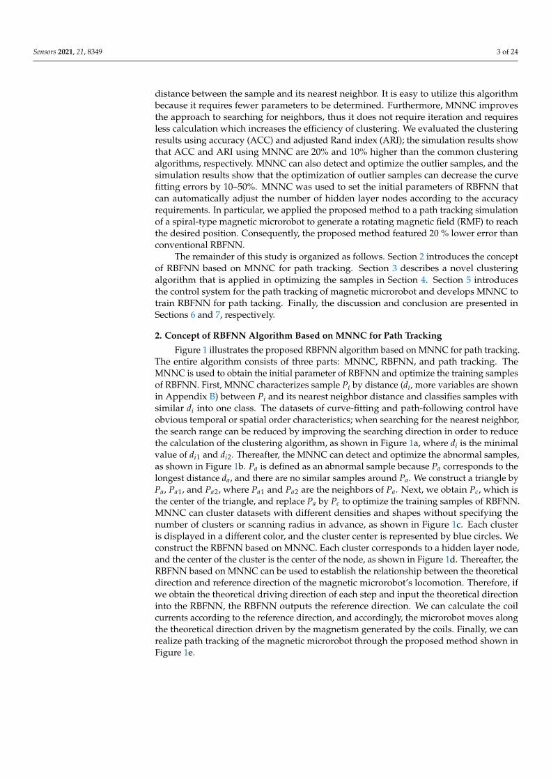
Figure 1 illustrates the proposed RBFNN algorithm based on MNNC for path tracking.The entire algorithm consists of three parts: MNNC, RBFNN, and path tracking. TheMNNC is used to obtain the initial parameter of RBFNN and optimize the training samplesof RBFNN. First, MNNC characterizes sample Pi by distance (di, more variables are shownin Appendix B) between Pi and its nearest neighbor distance and classifies samples withsimilar di into one class. The datasets of curve-fitting and path-following control haveobvious temporal or spatial order characteristics; when searching for the nearest neighbor,the search range can be reduced by improving the searching direction in order to reducethe calculation of the clustering algorithm, as shown in Figure 1a, where di is the minimalvalue of di1 and di2. Thereafter, the MNNC can detect and optimize the abnormal samples,as shown in Figure 1b. Pa is defined as an abnormal sample because Pa corresponds to thelongest distance da, and there are no similar samples around Pa. We construct a triangle byPa, Pa1, and Pa2, where Pa1 and Pa2 are the neighbors of Pa. Next, we obtain Pc, which isthe center of the triangle, and replace Pa by Pc to optimize the training samples of RBFNN.MNNC can cluster datasets with different densities and shapes without specifying thenumber of clusters or scanning radius in advance, as shown in Figure 1c. Each clusteris displayed in a different color, and the cluster center is represented by blue circles. Weconstruct the RBFNN based on MNNC. Each cluster corresponds to a hidden layer node,and the center of the cluster is the center of the node, as shown in Figure 1d. Thereafter, theRBFNN based on MNNC can be used to establish the relationship between the theoreticaldirection and reference direction of the magnetic microrobot’s locomotion. Therefore, ifwe obtain the theoretical driving direction of each step and input the theoretical directioninto the RBFNN, the RBFNN outputs the reference direction. We can calculate the coilcurrents according to the reference direction, and accordingly, the microrobot moves alongthe theoretical direction driven by the magnetism generated by the coils. Finally, we canrealize path tracking of the magnetic microrobot through the proposed method shown inFigure 1e.

Sensors 2021, 21, 8349 4 of 24Sensors 2021, 21, x FOR PEER REVIEW 4 of 27

Figure 1. Concept of an RBFNN algorithm based on MNNC for path tracking: (a) calculation of the distance to obtain the nearest neighbor; (b) detection of the abnormal samples based on nearest neighbor method; (c) clustering of the samples based on the nearest neighbor; (d) construction of the RBFNN based on MNNC; (e) obtaining the reference position by the MNNC-based RBFNN in the path tracking system.

3. Clustering Algorithm Based on Nearest Neighbor 3.1. Typical Clustering Algorithm

A clustering algorithm is a typical unsupervised learning algorithm that is mainly used to automatically classify similar samples into a specific category. The main clustering methods can be divided into five methods: the partitioning method, hierarchical method, grid-based method, model-based method, and density-based method [24]. The partition method decomposes the data into n clusters, such that the items in each cluster are closely related to each other, for example, K-means algorithm. The calculation procedure in this algorithm is simple, but it is necessary to know the number of clusters of data in advance [25].

Balanced iterative reducing and clustering using hierarchies (BIRCH) is a typical representative of the hierarchical method that decomposes a given dataset hierarchically until a certain condition is met. Specifically, it can be categorized into “bottom-up” and “top-down” schemes [26]. This algorithm is not particularly suitable for non-convex datasets, and owing to the limit on the number of each node, the clustering result may deviate from the actual classification.

Clustering in QUEst (CLIQUE) is a clustering algorithm based on the grid method. In this algorithm, the data space is first divided into a grid structure of finite units, and all processing is based on a single unit. This algorithm is highly sensitive to parameters and cannot handle irregularly distributed data [27]. There is no iteration required in this method, but it is difficult to determine the density threshold, an important parameter in the algorithm. Model-based methods set a model for each cluster, and subsequently detect a dataset that satisfies this model adequately. Such a model may be the density distribution function of data points in space or other. The efficiency of this algorithm also needs to be improved [28]. The model-based method incorporates the probability and statistics approach and the neural network approach.

Density-based methods attempt to determine the high-density clusters separated by sparse regions. The size and shape of these clusters may be different. The most commonly used clustering algorithm based on density is DBSCAN. Although this algorithm does not necessitate knowledge of the number of classes the data is divided into in advance, knowledge of the radius and the minimum number of points is required [29].

Figure 1. Concept of an RBFNN algorithm based on MNNC for path tracking: (a) calculation of the distance to obtain thenearest neighbor; (b) detection of the abnormal samples based on nearest neighbor method; (c) clustering of the samplesbased on the nearest neighbor; (d) construction of the RBFNN based on MNNC; (e) obtaining the reference position by theMNNC-based RBFNN in the path tracking system.

3. Clustering Algorithm Based on Nearest Neighbor3.1. Typical Clustering Algorithm

A clustering algorithm is a typical unsupervised learning algorithm that is mainlyused to automatically classify similar samples into a specific category. The main clusteringmethods can be divided into five methods: the partitioning method, hierarchical method,grid-based method, model-based method, and density-based method [24]. The partitionmethod decomposes the data into n clusters, such that the items in each cluster are closelyrelated to each other, for example, K-means algorithm. The calculation procedure inthis algorithm is simple, but it is necessary to know the number of clusters of data inadvance [25].

Balanced iterative reducing and clustering using hierarchies (BIRCH) is a typicalrepresentative of the hierarchical method that decomposes a given dataset hierarchicallyuntil a certain condition is met. Specifically, it can be categorized into “bottom-up” and “top-down” schemes [26]. This algorithm is not particularly suitable for non-convex datasets,and owing to the limit on the number of each node, the clustering result may deviate fromthe actual classification.

Clustering in QUEst (CLIQUE) is a clustering algorithm based on the grid method.In this algorithm, the data space is first divided into a grid structure of finite units, andall processing is based on a single unit. This algorithm is highly sensitive to parametersand cannot handle irregularly distributed data [27]. There is no iteration required in thismethod, but it is difficult to determine the density threshold, an important parameter inthe algorithm. Model-based methods set a model for each cluster, and subsequently detecta dataset that satisfies this model adequately. Such a model may be the density distributionfunction of data points in space or other. The efficiency of this algorithm also needs tobe improved [28]. The model-based method incorporates the probability and statisticsapproach and the neural network approach.

Density-based methods attempt to determine the high-density clusters separated bysparse regions. The size and shape of these clusters may be different. The most commonlyused clustering algorithm based on density is DBSCAN. Although this algorithm doesnot necessitate knowledge of the number of classes the data is divided into in advance,knowledge of the radius and the minimum number of points is required [29].

Sensors 2021, 21, 8349 5 of 24

3.2. Modified Nearest Neighbor-Based Clustering Algorithm for Training RBFNN

When we train the RBFNN for curve fitting and path tracking to obtain the structureparameters, clustering the training data to determine the center and number of basisfunctions of the hidden layer is an effective approach. The dataset in this case featuresobvious time or space characteristics. Here, we propose a simple clustering algorithmMNNC that clusters the samples according to the distance (di) between the sample and itsnearest neighbor, as shown in Figure 2 and Definition 1. Adjacent samples with similar diare categorized into the same cluster, and the method of searching for the nearest neighboris modified. Only the distance between the sample and the preceding and the followingsamples needs to be calculated according to the property of the RBFNN training dataset.Thus, the calculation is significantly less than the other clustering algorithms, and only asingle MNNC parameter requires to be determined.

Sensors 2021, 21, x FOR PEER REVIEW 5 of 27

3.2. Modified Nearest Neighbor-Based Clustering Algorithm for Training RBFNN When we train the RBFNN for curve fitting and path tracking to obtain the structure

parameters, clustering the training data to determine the center and number of basis functions of the hidden layer is an effective approach. The dataset in this case features obvious time or space characteristics. Here, we propose a simple clustering algorithm MNNC that clusters the samples according to the distance (di) between the sample and its nearest neighbor, as shown in Figure 2 and Definition 1. Adjacent samples with similar di are categorized into the same cluster, and the method of searching for the nearest neighbor is modified. Only the distance between the sample and the preceding and the following samples needs to be calculated according to the property of the RBFNN training dataset. Thus, the calculation is significantly less than the other clustering algorithms, and only a single MNNC parameter requires to be determined.

Figure 2. Sample distribution: (a) the training samples are dispersed with spatial sequence; (b) the training samples are dispersed without spatial sequence.

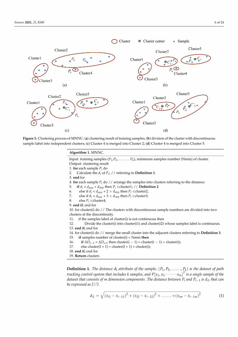
The basic principle of the clustering algorithm is that similar samples are placed in the same cluster, where the similarity of two samples is described by the Euclidean distance of the two samples. Since the sample has the characteristics of time series, the nearest samples to sample iP are the adjacent samples 1iP− and 1iP+ , as shown in Figure 2a. The distances between the samples are 1id and 2id , respectively, thus the nearest distance, id , of iP is the smaller of [ 1id , 2id ]. The calculation of this method is simpler than that of the other clustering algorithms. Thereafter, id is divided into different levels, and the samples with the same id level belong to the same cluster (Figure 3a).

If the samples in one cluster are not adjacent, as shown in Figure 3a (where 8P and 10P are not adjacent samples), the cluster is divided at the breakpoint (Figure 3b). Finally,

the small clusters are merged with the adjacent clusters, as shown in Figure 3c,d. The merging criterion is that the total distance change ( DΔ ) between all samples and the centroid should be the least, such that the adjacent samples with the similar distance characteristic form a cluster. The related definitions are executed in Algorithm 1 for the distance (di), distance step (dstep), and distance changes ( DΔ ).

Figure 2. Sample distribution: (a) the training samples are dispersed with spatial sequence; (b) thetraining samples are dispersed without spatial sequence.

The basic principle of the clustering algorithm is that similar samples are placed in thesame cluster, where the similarity of two samples is described by the Euclidean distanceof the two samples. Since the sample has the characteristics of time series, the nearestsamples to sample Pi are the adjacent samples Pi−1 and Pi+1, as shown in Figure 2a. Thedistances between the samples are di1 and di2, respectively, thus the nearest distance, di, ofPi is the smaller of [di1,di2]. The calculation of this method is simpler than that of the otherclustering algorithms. Thereafter, di is divided into different levels, and the samples withthe same di level belong to the same cluster (Figure 3a).

If the samples in one cluster are not adjacent, as shown in Figure 3a (where P8 and P10are not adjacent samples), the cluster is divided at the breakpoint (Figure 3b). Finally, thesmall clusters are merged with the adjacent clusters, as shown in Figure 3c,d. The mergingcriterion is that the total distance change (∆D) between all samples and the centroid shouldbe the least, such that the adjacent samples with the similar distance characteristic form acluster. The related definitions are executed in Algorithm 1 for the distance (di), distancestep (dstep), and distance changes (∆D).

Sensors 2021, 21, 8349 6 of 24Sensors 2021, 21, x FOR PEER REVIEW 6 of 27

Figure 3. Clustering process of MNNC: (a) clustering result of training samples; (b) division of the cluster with discontinuous sample label into independent clusters; (c) Cluster 4 is merged into Cluster 2; (d) Cluster 4 is merged into Cluster 5.

Algorithm 1. MNNC. Input: training samples 1 2( , , ......, )kP P P , minimum samples number (Nmin) of cluster. Output: clustering result 1. for each sample Pi do 2. Calculate the di of Pi; // referring to Definition 1. 3. end for 4. for each sample Pi do // arrange the samples into clusters referring to the distance. 5. if di < dmin + dstep then Pi ∈cluster1; // Definition 2 6. else if di < dmin + 2×dstep then Pi ∈cluster2; 7. else if di < dmin + 3×dstep then Pi ∈cluster3; 8. else Pi ∈cluster4; 9. end if; end for 10. for cluster(i) do // The clusters with discontinuous sample numbers are divided into two clusters at the discontinuity. 11. if the samples label of cluster(i) is not continuous then 12. Divide the cluster(i) into cluster(i1) and cluster(i2) whose samples label is continuous. 13. end if; end for 14. for cluster(i) do // merge the small cluster into the adjacent clusters referring to Definition 3. 15. if samples number of cluster(i) < Nmin then 16. if 1iD −Δ < 1iD +Δ then cluster(i − 1)= cluster(i − 1)+ cluster(i); 17. else cluster(I + 1) = cluster(I + 1) + cluster(i); 18. end if; end for 19. Return clusters

Definition 1. The distance di attribute of the sample, 1 2( , , ......, )kP P P is the dataset of path tracking control system that includes k samples, and [ ]1 2, T

mP x x x⋅ ⋅⋅ ⋅ ⋅⋅ is a single sample of the dataset that consists of m dimension components. The distance betweeniP and 1iP− is 1id that can be expressed as [17]

Figure 3. Clustering process of MNNC: (a) clustering result of training samples; (b) division of the cluster with discontinuoussample label into independent clusters; (c) Cluster 4 is merged into Cluster 2; (d) Cluster 4 is merged into Cluster 5.

Algorithm 1. MNNC.

Input: training samples (P1,P2, . . . . . . Pk), minimum samples number (Nmin) of cluster.Output: clustering result1. for each sample Pi do2. Calculate the di of Pi; // referring to Definition 1.3. end for4. for each sample Pi do // arrange the samples into clusters referring to the distance.5. if di < dmin + dstep then Pi ∈cluster1; // Definition 26. else if di < dmin + 2 × dstep then Pi ∈cluster2;7. else if di < dmin + 3 × dstep then Pi ∈cluster3;8. else Pi ∈cluster4;9. end if; end for10. for cluster(i) do // The clusters with discontinuous sample numbers are divided into twoclusters at the discontinuity.11. if the samples label of cluster(i) is not continuous then12. Divide the cluster(i) into cluster(i1) and cluster(i2) whose samples label is continuous.13. end if; end for14. for cluster(i) do // merge the small cluster into the adjacent clusters referring to Definition 3.15. if samples number of cluster(i) < Nmin then16. if ∆Di−1 < ∆Di+1 then cluster(i − 1) = cluster(i − 1) + cluster(i);17. else cluster(I + 1) = cluster(I + 1) + cluster(i);18. end if; end for19. Return clusters

Definition 1. The distance di attribute of the sample, (P1, P2, . . . . . ., Pk) is the dataset of pathtracking control system that includes k samples, and P[x1, x2 · · · · · ·xm]

T is a single sample of thedataset that consists of m dimension components. The distance between Pi and Pi−1 is di1 that canbe expressed as [17]

di1 =

√(xi1 − xi−11)

2 + (xi2 − xi−12)2 + . . . . . .+(xim − xi−1m)

2 (1)

Sensors 2021, 21, 8349 7 of 24

The distance between Pi and Pi+1 is di2 that can be expressed as

di2 =

√(xi1 − xi+11)

2 + (xi2 − xi+12)2 + . . . . . .+(xim − xi+1m)

2 (2)

The minimal distance di among (di1, di2) is expressed as

di = min(di1, di2) (3)

Definition 2. Distance step (dstep) (d1, d2, . . . . . ., dk) is the distance of the sample (P1, P2, . . . . . ., Pk).

dmax = max(d1, d2, . . . . . ., dk) (4)

dmin = min(d1, d2, . . . . . ., dk) (5)

The distance step is calculated as follows, where H is the number of di level determined bythe user.

dstep =dmax − dmin

H(6)

Definition 3. Distance change (∆D)The total distance of Cluster 2 and Cluster 5 (Figure 3b) is calculated before the merge operation.

D2 = ∑Quan2i=1 ‖Pi − C2‖

2(7)

D5 = ∑Quan5i=1 ‖Pi − C5‖

2(8)

where Quan2 and Quan5 are the quantity of samples in Cluster 2 and Cluster 5, respectively, andC2 and C5 are the centers of Cluster 2 and Cluster 5 as shown in Figure 3b, respectively; the centerof Cluster 2 can be determined using Equation (9), and we can obtain the centers of the other clusterssimilarly.

C2m =x1m + x2m + . . . . . .+xUm

U(9)

where C2m is the component m of the center of Cluster 2, and x1m is the component m of sample 1of Cluster 2. The total distances of Cluster 2 and Cluster 5 are calculated after the merge operation.If Cluster 4 is merged into Cluster 2, the center of Cluster 2 becomes C2′ , as shown in Figure 3c.

D′2 = ∑U′

i=1 ‖Pi − C′2‖2

(10)

If Cluster 4 is merged into Cluster 5, the center of Cluster 5 becomes C5′ , as shown inFigure 3d.

D′5 = ∑V′

i=1 ‖Pi − C′5‖2

(11)

Therefore, the distance change (∆D) is

∆D2 =∣∣D′2 − D2

∣∣ (12)

∆D5 =∣∣D′5 − D5

∣∣ (13)

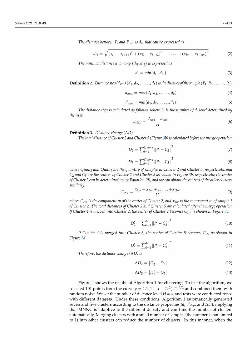
Figure 4 shows the results of Algorithm 1 for clustering. To test the algorithm, weselected 101 points from the curve y = 1.1(1− x + 2x2)e−x2/2 and combined them withrandom noise. We set the number of distance level H = 4, and tests were conducted twicewith different datasets. Under these conditions, Algorithm 1 automatically generatedseven and five clusters according to the distance properties (di, dstep, and ∆D), implyingthat MNNC is adaptive to the different density and can tune the number of clustersautomatically. Merging clusters with a small number of samples (the number is not limitedto 1) into other clusters can reduce the number of clusters. In this manner, when the

Sensors 2021, 21, 8349 8 of 24

clustering algorithm is applied along with other intelligent algorithms, the speed of theintelligent algorithm can be improved.

Sensors 2021, 21, x FOR PEER REVIEW 8 of 27

5 5 5'D D DΔ = − (13)

Figure 4 shows the results of Algorithm_1 for clustering. To test the algorithm, we

selected 101 points from the curve 22 /21.1(1 2 ) xy x x e−= − + and combined them with

random noise. We set the number of distance level H = 4, and tests were conducted twice with different datasets. Under these conditions, Algorithm 1 automatically generated seven and five clusters according to the distance properties (di, dstep, and DΔ ), implying that MNNC is adaptive to the different density and can tune the number of clusters automatically. Merging clusters with a small number of samples (the number is not limited to 1) into other clusters can reduce the number of clusters. In this manner, when the clustering algorithm is applied along with other intelligent algorithms, the speed of the intelligent algorithm can be improved.

Figure 4. Clustering results: (a) the training samples are divided into seven clusters; (b) the training samples are divided into five clusters.

3.3. Enhancement of MNNC Performance The clustering algorithm can use the samples with a time sequence or spatial

sequence, as shown in Figure 2a; the nearest neighbor of sample Pi is either Pi-1 or Pi+1. This clustering algorithm is suitable for curve fitting and path tracking control. Furthermore, the samples are randomly distributed without the time and spatial sequences, as shown in Figure 2b. In this case, the nearest neighbor of Pi may be in any direction, and we need to calculate the distances from Pi to its neighbors for determining id . The detailed calculation is shown in Definition 4. After we obtain the distances 1 2( , , ......, )kd d d , that is, the id of the samples, we set max 1 2min( , , ......, )kd d d d= . Thereafter, the sample Pm is determined, whose distance to Pi is less than maxd . These samples and Pi form a neighbor cluster of Pi. Similarly, the neighbor clusters of the other samples can be established. If the sample Pmax owns the distance attribute of dmax, and its neighbor cluster contains only two samples, we define Pmax as an abnormal sample and delete this sample. Next, we set the updated maximum distance, and subsequently establish the neighbor cluster of each sample again. If there are several neighbor clusters containing the same samples, then these neighbor clusters merge into one cluster. The execution process proceeds based on Algorithm 2.

Definition 4. Distance attribute of the sample ( id ): To reduce the calculation, the samples are sorted by x and y, respectively. Px1 and Px2 are the preceding and following samples relative to sample Pi, sorted by x. Py1 and Py2 are the preceding and following samples relative to sample Pi sorted by y. dx1, dx2, dy1, and dγ2 are the distances between Pi and Px1, Px2, Py1, and Py2, respectively.

( ) ( )2 21 1 1x x i x id x x y y= − + − (14)

Figure 4. Clustering results: (a) the training samples are divided into seven clusters; (b) the trainingsamples are divided into five clusters.

3.3. Enhancement of MNNC Performance

The clustering algorithm can use the samples with a time sequence or spatial sequence,as shown in Figure 2a; the nearest neighbor of sample Pi is either Pi−1 or Pi+1. Thisclustering algorithm is suitable for curve fitting and path tracking control. Furthermore,the samples are randomly distributed without the time and spatial sequences, as shown inFigure 2b. In this case, the nearest neighbor of Pi may be in any direction, and we need tocalculate the distances from Pi to its neighbors for determining di. The detailed calculationis shown in Definition 4. After we obtain the distances (d1, d2, . . . . . ., dk), that is, the di ofthe samples, we set dmax = min(d1, d2, . . . . . ., dk). Thereafter, the sample Pm is determined,whose distance to Pi is less than dmax. These samples and Pi form a neighbor cluster of Pi.Similarly, the neighbor clusters of the other samples can be established. If the sample Pmaxowns the distance attribute of dmax, and its neighbor cluster contains only two samples,we define Pmax as an abnormal sample and delete this sample. Next, we set the updatedmaximum distance, and subsequently establish the neighbor cluster of each sample again.If there are several neighbor clusters containing the same samples, then these neighborclusters merge into one cluster. The execution process proceeds based on Algorithm 2.

Definition 4. Distance attribute of the sample (di): To reduce the calculation, the samples are sortedby x and y, respectively. Px1 and Px2 are the preceding and following samples relative to sample Pi,sorted by x. Py1 and Py2 are the preceding and following samples relative to sample Pi sorted by y.dx1, dx2, dy1, and dγ2 are the distances between Pi and Px1, Px2, Py1, and Py2, respectively.

dx1 =

√(xx1 − xi)

2 + (yx1 − yi)2 (14)

dx2 =

√(xx2 − xi)

2 + (yx2 − yi)2 (15)

dy1 =√(

xy1 − xi)2

+(yy1 − yi

)2 (16)

dy2 =√(

xy2 − xi)2

+(yy2 − yi

)2 (17)

di0 can be expressed asdi0 = min(dx1, dx2, dy1, dy2) (18)

The sample Pj; xj and yj of Pj satisfy∣∣xj − xi∣∣ ≤ di0 (19)∣∣yj − yi∣∣ ≤ di0 (20)

Sensors 2021, 21, 8349 9 of 24

The distance between Pj and Pi: can be calculated using

dj =√(

xj − xi)2

+(yj − yi

)2 (21)

Finally, the distance attribute of Pi is

di = min(d1, d2, . . . . . ., dj) (22)

Algorithm 2. MNNC for the path tracking of magnetic microrobot.

Input: training samples (P1,P2, . . . . . . Pk).Output: clustering result.1. for each sample Pi do2. Calculate the di of Pi; // referring to Definition 4.3. end for4. dmax = max(d1,d2, . . . . . . dk); dmin = min(d1,d2, . . . . . . dk);5. dstep = (dmax + dmin)/H; //H is distance level number that is determined by user.6. for each distance level;7. for each sample Pi do // find the nearest neighbors of Pi and establish the neighbor clusers.8. Find the smaple Pm which ‖Pm−Pi‖ ≤ dmin + H × dstep;9. Construct cluster(i) = (Pi, Pm);10. end for11. for each cluster(i) do // if clusters contain same sample, then merge these clusters into onecluster.12. If cluster(i) ∩ cluster(j) 6= Ø then cluster(i) = cluster(i) + cluster(j);13. end if; end for14. end for15. merge the small cluster into nearest cluster16. Return clusters

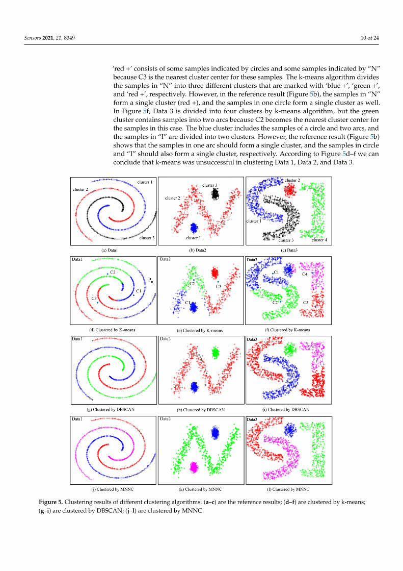
It can be observed from the previous steps that MNNC for path tracking does notrequire us to pre-select important parameters based on experience. Because there is noiterative process, the calculation is not large in the algorithm. Furthermore, this clusteringalgorithm is also suitable for multi-dimensional samples. To verify the effectiveness ofthe clustering algorithm, we used MNNC, K-means, and DBSCAN to perform clusteringanalysis on the same samples, as shown in Figure 5.

We generated three synthetic datasets called Data 1 (Figure 5a), Data 2 (Figure 5b), andData 3 (Figure 5c) containing 600, 1001, and 1650 samples, respectively. Data 1 consists ofthree clusters that are marked with ‘blue +’, ‘red +’, and ‘black +’, respectively. Data 2 alsoconsists of three clusters that are marked with ‘blue +’, ‘red +’, and ‘black +’, respectively.Data3 consists of four clusters that are marked with ‘blue +’, ‘red +’, ‘black +’, and ‘green +’,respectively.

Figure 5d–f are the clustering results of Data 1, Data 2, and Data 3 obtained by k-means,respectively. Prior to the cluster analysis of Data 1, Data 2, and Data 3 by k-means, we setthe parameter K to 3, 3, and 4, respectively, but the clustering results still remain incorrect.

Data 1 was divided into three clusters that were marked with ‘blue +’, ‘green +’, and‘red +’, as shown in Figure 5d. As the reference result in Figure 5a shows, the samples ofevery cluster form a spiral. However, the cluster formations were changed when Data 1was clustered by k-means. The changed cluster formed around each center of the clusters(C1, C2, and C3); blue cluster is the area around C1, green cluster is the area around C2, thered cluster is the area around C3. This is because of the principle of k-means that clustersthe dataset based on the distance between samples and cluster centers. For example, weassume that C1, C2, and C3 are the centers of blue, green, and red clusters, respectively.Pn is any sample of the blue cluster, as shown in Figure 5d. For the sample Pn, C1 is thenearest cluster center among C1, C2, and C3. Therefore, sample Pn becomes one of thesamples of the blue cluster. Similar results are shown in Figure 5e. The cluster marked with

Sensors 2021, 21, 8349 10 of 24

‘red +’ consists of some samples indicated by circles and some samples indicated by “N”because C3 is the nearest cluster center for these samples. The k-means algorithm dividesthe samples in “N” into three different clusters that are marked with ‘blue +’, ‘green +’,and ‘red +’, respectively. However, in the reference result (Figure 5b), the samples in “N”form a single cluster (red +), and the samples in one circle form a single cluster as well.In Figure 5f, Data 3 is divided into four clusters by k-means algorithm, but the greencluster contains samples into two arcs because C2 becomes the nearest cluster center forthe samples in this case. The blue cluster includes the samples of a circle and two arcs, andthe samples in “I” are divided into two clusters. However, the reference result (Figure 5b)shows that the samples in one arc should form a single cluster, and the samples in circleand “I” should also form a single cluster, respectively. According to Figure 5d–f we canconclude that k-means was unsuccessful in clustering Data 1, Data 2, and Data 3.

Sensors 2021, 21, x FOR PEER REVIEW 10 of 27

Figure 5. Clustering results of different clustering algorithms: (a–c) are the reference results; (d–f) are clustered by k-means; (g–i) are clustered by DBSCAN; (j–l) are clustered by MNNC.

We generated three synthetic datasets called Data 1 (Figure 5a), Data 2 (Figure 5b), and Data 3 (Figure 5c) containing 600, 1001, and 1650 samples, respectively. Data 1 consists of three clusters that are marked with ‘blue +’, ‘red +’, and ‘black +’, respectively. Data 2 also consists of three clusters that are marked with ‘blue +’, ‘red +’, and ‘black +’, respectively. Data3 consists of four clusters that are marked with ‘blue +’, ‘red +’, ‘black +’, and ‘green +’, respectively.

Figure 5d–f are the clustering results of Data 1, Data 2, and Data 3 obtained by k-means, respectively. Prior to the cluster analysis of Data 1, Data 2, and Data 3 by k-means, we set the parameter K to 3, 3, and 4, respectively, but the clustering results still remain incorrect.

Figure 5. Clustering results of different clustering algorithms: (a–c) are the reference results; (d–f) are clustered by k-means;(g–i) are clustered by DBSCAN; (j–l) are clustered by MNNC.

Sensors 2021, 21, 8349 11 of 24

During the simulation, we set R (scanning radius) of DBSCAN equal to the maximumdistance (dmax) of MNNC, and set the same Mp (minimal points number) for Data 1, Data 2,and Data 3. The clustering results of Data 1, Data 2, and Data 3 by DBSCAN are shown inFigure 5g–i respectively. As shown in Figure 5g, DBSCAN divided Data 1 into three clustersprecisely, as shown in Figure 5g; it placed the samples of one spiral in an independentcluster. DBSCAN generated three clusters for Data 2, as shown in Figure 5h; the threeclusters were marked with ‘blue +’, ‘green +’, and ‘red +’, respectively. However, as shownin Figure 5i DBSCAN divided the samples in “I” into two clusters that were marked with‘pink +’, and ‘black +’. The clustering result of Data 3 by DBSCAN is not equivalent tothe reference result for Data 3 that shows that the samples in “I” belong to a single cluster.This is because DBSCAN not only depends on the parameter R, but also on the parameterMp. However, at this time, Mp is not suitable for Data 3 anymore, implying that we shoulddefine two correct parameters of DBSCAN for different cases based on experience.

Figure 5j–l are the clustering results of Data 1, Data 2, and Data 3 usingMNNC,respectively. Figure 5j,k show that MNNC generated equivalent clusters for Data 1 andData 2. MNNC divided the samples of Data 1 and Data 2 into three clusters that weremarked with ‘blue +’, ‘green +’, and ‘red +’, respectively. MNNC almost clustered Data 3correctly, except it regarded one sample in “I” as an abnormal sample (marked with“black ×”), as shown in Figure 5l. This is because the sample, marked with “black ×”,features the largest di, and there are no similar samples around it.

Therefore, we can conclude that MNNC features the best clustering function for thesedatasets. Simultaneously, MNNC does not require users to decide the parameters, whereasboth DBSCAN and k-mean require users to define two parameters. To clearly describe theclustering results, we used ACC and ARI to evaluate the clustering results [30]. The resultsare shown in Table 1.

As shown in Table 1, the ACC and ARI of three datasets of k-means clustering aremuch smaller than those of DBSCAN and MNNC, implying that the clustering results byk-means are lower than those obtained by DBSCAN and MNNC. The ACC and ARI ofthe spiral and zigzag of DBSCAN and MNNC are all 1, indicating that both DBSCAN andMNNC cluster those two datasets precisely. The ACC index of C4 of DBSCAN and MNNCare 0.8558 and 0.9994, respectively. The ARI index of C4 by DBSCAN and MNNC are0.9019 and 0.9994, respectively. Both indexes of DBSCAN are smaller than those of MNNCwhich implies that the clustering results of MNNC are better than those of DBSCAN. Theresult of clustering index is similar to the clustering result, as shown in Figure 5.

Table 1. Clustering index of the clustering results.

ClusteringAlgorithm

PerformanceIndex

Dataset

Data 1 Data 2 Data 3

K-meansACC 0.3333 0.6683 0.4891ARI 0.0233 0.3121 0.3010

DBSCANACC 1 1 0.8558ARI 1 1 0.9019

MNNCACC 1 1 0.9994ARI 1 1 0.9994

4. Adjustment of Training Samples Based on MNNC

The abnormal samples can be optimized by unsupervised methods before the in-telligent algorithm parameters are defined. Therefore, the unsupervised methods cansignificantly improve the predictive ability of intelligent algorithm models [31]. Abnormaltraining samples always affect the operating efficiency of neural networks [32]; it is neces-sary to detect the abnormal samples and treat them. Training samples for the path trackingsystem with abnormal samples are shown in Figure 6a. The abnormal samples are markedas stars that reduce the learning effect of the algorithm for path tacking such as RBFNN.We can detect the abnormal samples by MNNC that requires fewer parameters than the

Sensors 2021, 21, 8349 12 of 24

other algorithms. After defining the abnormal samples, we can delete them directly, but itis not particularly effective for curve fitting or path tracking control.

Sensors 2021, 21, x FOR PEER REVIEW 13 of 27

Figure 6. (a) Scheme of analysis of abnormal sample; (b) curve fitting results.

We tested the effect of training sample adjustment. The training samples were obtained from different curves that were combined with random noise or some specific noise. The results are shown in Figure 6b and summarized in Table 2. From Figure 6b and Table 2, we can observe that the fitting errors of the 2D curve mixed with random noise are 3.0793 when the abnormal samples are not adjusted; but the fitting errors of the same dataset are only 2.8145 after the abnormal samples are adjusted. Furthermore, the fitting errors of the 2D curve mixed with six noise points without and with abnormal sample adjustment are 2.7281 and 1.3292, respectively. The modified effect of the 3D curve is not comparable to that of the 2D curve; the fitting errors decrease from 516.6542 to 485.3374. Therefore, we can conclude that the adjustment of abnormal samples can improve the curve fitting accuracy. Particularly, the accuracy is improved by approximately 50% when there are only six abnormal samples. Because these six abnormal samples deviate far from the normal samples, these six samples change considerably after they are adjusted to normal samples. Therefore, the accuracy of the entire curve fitting is significantly improved. All the simulations were performed in Matlab.

Table 2. Errors of curve fitting with/without the adjustment of abnormal samples.

Curve Type 2D Curve 3D Curve

Noise style Randomly distributed

Six points with noise Randomly distributed

Errors without adjustment

3.0793 2.7281 516.6542

Errors with adjustment 2.8145 1.3292 485.3374

Figure 6. (a) Scheme of analysis of abnormal sample; (b) curve fitting results.

Particularly, when the number of training samples is not large, insufficient trainingsamples also reduce the accuracy of RBFNN. It is effective to adjust the abnormal samples tonormal samples. The process of detecting and adjusting abnormal samples is performed byMNNC. First, the training samples are clustered by MNNC. There are some independentsamples because they are far away from the neighbors, such as P1 and P2 that are theabnormal and normal samples, respectively. We should distinguish between P1 and P2.Therefore, a triangle is formed by the samples of P1, Pf , and Pb. The samples Pf and Pbare neighbors of P1, as shown in Figure 6a. Thereafter, we calculate the distance from thecenter of the triangle (Pc) to P1, Pf , and Pb, respectively. On one hand, if the distance (dc_1)between Pc and P1 is not larger than that of Pf and Pb, we define P1 as a normal sample.On the other hand, when the dc_1 is larger than that of Pf and Pb, the sample P1 becomesthe abnormal sample and moves to Pc.

We tested the effect of training sample adjustment. The training samples were obtainedfrom different curves that were combined with random noise or some specific noise. Theresults are shown in Figure 6b and summarized in Table 2. From Figure 6b and Table 2,we can observe that the fitting errors of the 2D curve mixed with random noise are 3.0793when the abnormal samples are not adjusted; but the fitting errors of the same dataset areonly 2.8145 after the abnormal samples are adjusted. Furthermore, the fitting errors ofthe 2D curve mixed with six noise points without and with abnormal sample adjustmentare 2.7281 and 1.3292, respectively. The modified effect of the 3D curve is not comparableto that of the 2D curve; the fitting errors decrease from 516.6542 to 485.3374. Therefore,we can conclude that the adjustment of abnormal samples can improve the curve fittingaccuracy. Particularly, the accuracy is improved by approximately 50% when there areonly six abnormal samples. Because these six abnormal samples deviate far from the

Sensors 2021, 21, 8349 13 of 24

normal samples, these six samples change considerably after they are adjusted to normalsamples. Therefore, the accuracy of the entire curve fitting is significantly improved. Allthe simulations were performed in Matlab.

Table 2. Errors of curve fitting with/without the adjustment of abnormal samples.

Curve Type 2D Curve 3D Curve

Noise style Randomly distributed Six points with noise Randomly distributedErrors without

adjustment 3.0793 2.7281 516.6542

Errors withadjustment 2.8145 1.3292 485.3374

5. Application of RBFNN in Path Tracking for a Spiral-Type Magnetic Microrobot

Figure 7a shows the control method of a spiral-type magnetic microrobot usingrotating magnetic field (RMF) control. The robot is synchronized by the applied RMF anddriven by magnetic torque. A rotation of the robot generates propulsive force via the screwmechanism. The driving magnetic torque Tm can be expressed as follows [33]:

Tm = VM× B (23)

where V is the volume of microrobot, M is the magnetization, and B is the external magneticflux density. The magnetized direction of the robot is the radial direction. The externalmagnetic field is a uniform RMF and is generated by a three-axis Helmholtz coil. Weassume that a magnetic field B generated by 3D Helmholtz coils rotates in plane P. Thus,the normal vector (nB) of plane P represents the movement direction of the robot. Inaddition, because the control angles of γ and α determine the position of plane P, thecontrol of two angles determines the steering of the robot. The normal vector nB andmagnetic field B can be described as follows:

nB = [sin(γ) cos(α), sin(γ) sin(α), cos(γ)]T (24)

B =

BxByBz

= B0

cos(γ) cos(α) sin(ωt) + sin(α) cos(ωt)cos(γ) sin(α) sin(ωt)− cos(α) cos(ωt)

− sin(γ) sin(ωt)

(25)

where B0 is the norm of B; γ is the polar angle, and α is the azimuthal angle.

Sensors 2021, 21, x FOR PEER REVIEW 15 of 27

establish the relationship between the reference ( refγ and refα) and control angles ( γ cont

and αcont ) after it is trained.

Figure 7. (a) Magnetic field vector; (b) scheme of path tracking: the green arrow is the reference direction, the red arrow is the desired direction, and the yellow arrow is.

Generally, RBFNN includes three layers: input, hidden, and output layers, as shown in Figure 8a. In this study, we used MNNC to train the RBFNN to develop its structure.

Figure 8. Scheme of RBFNN and control system: (a) structure of RBFNN for path tracking; (b) flow chart of control system.

The input layer of RBFNN includes two neurons: reference angle refγ and refα.

The number of neuron and center of hidden layer are determined by MNNC after the RBFNN is trained. Accordingly, the output of the hidden layer can be obtained as

2

22

( , )

n

cref ref n

Q e

σ

γ α

−

−

=

(26)

where cn is the center of hidden layer neurons that is decided by the MNNC. σ is the width of basis function that can be expressed as [37].

Figure 7. (a) Magnetic field vector; (b) scheme of path tracking: the green arrow is the guidance direction, the red arrowis the desired direction, the yellow arrow is the predicted direction, the blue arrow is the control direction, and the blackarrow is the actual directions.

Sensors 2021, 21, 8349 14 of 24

We assume that there are control errors resulting from various environmental factors.When we plan to drive the robot from the present position Po to the reference targetposition Pre f 1 along the reference direction dre f 1, the robot may arrive at the actual positionPact because of locomotion error between the actual and reference positions. Therefore,when we drive the robot to move along the control direction dact1 to compensate for thelocomotion error, the robot may reach the position Pre f 1, as shown in Figure 7b. If there isno error between the actual and reference positions, the control direction dc1 is matched tothe reference direction dre f 1 by training RBFNN. Next, when the robot arrives the positionPre f 1, we can obtain the next reference target position Pre f 2 and the reference directiondre f 2. Because the locomotion error is different in each locomotion step, we can obtain thecorresponding compensation by driving the robot along the control direction. Therefore,driving the robot to move along the control direction dci, the robot can reach each referenceposition Pr along the reference path. To decide the steering direction of the robot along thereference direction, the two angles of γre f and αre f are input to the RBFNN, and we obtainthe actual control angles of γcont and αcont by RBFNN for the controlling plane of RMF. Toachieve this aim, it is necessary to develop a locomotion control system for the robot that is anonlinear system. For nonlinear locomotion control systems, some researchers use RBFNNto simulate dynamic models [34,35]. However, the large number of parameters of thesemethods make the control system highly complicated. The neural network controller is anonlinear mapping system; it has been proved that any smooth function can be representedby a three-layer neural network with sufficient hidden neurons [36]. Finally, RBFNN can beused to establish the relationship between the reference (γre f and αre f ) and control angles(γcont and αcont) after it is trained.

Generally, RBFNN includes three layers: input, hidden, and output layers, as shownin Figure 8a. In this study, we used MNNC to train the RBFNN to develop its structure.

Sensors 2021, 21, x FOR PEER REVIEW 15 of 27

establish the relationship between the reference ( refγ and refα) and control angles ( γ cont

and αcont ) after it is trained.

Figure 7. (a) Magnetic field vector; (b) scheme of path tracking: the green arrow is the reference direction, the red arrow is the desired direction, and the yellow arrow is.

Generally, RBFNN includes three layers: input, hidden, and output layers, as shown in Figure 8a. In this study, we used MNNC to train the RBFNN to develop its structure.

Figure 8. Scheme of RBFNN and control system: (a) structure of RBFNN for path tracking; (b) flow chart of control system.

The input layer of RBFNN includes two neurons: reference angle refγ and refα.

The number of neuron and center of hidden layer are determined by MNNC after the RBFNN is trained. Accordingly, the output of the hidden layer can be obtained as

2

22

( , )

n

cref ref n

Q e

σ

γ α

−

−

=

(26)

where cn is the center of hidden layer neurons that is decided by the MNNC. σ is the width of basis function that can be expressed as [37].

Figure 8. Scheme of RBFNN and control system: (a) structure of RBFNN for path tracking; (b) flowchart of control system.

The input layer of RBFNN includes two neurons: reference angle γre f and αre f . Thenumber of neuron and center of hidden layer are determined by MNNC after the RBFNNis trained. Accordingly, the output of the hidden layer can be obtained as

Qn = e

−‖(γre f ,αre f )−cn‖2

2σ2

(26)

where cn is the center of hidden layer neurons that is decided by the MNNC. σ is the widthof basis function that can be expressed as [37].

σ =dc√2n

(27)

Sensors 2021, 21, 8349 15 of 24

where dc is the maximum distance among the neuron centers of hidden layer; n is thequantity of neuron units of the hidden layer, and both of them can be obtained by MNNC.

The output layer includes two neurons: control angles of γcont and αcont. They can beobtained by RBFNN according to{

γcont = ∑ni=1 Qiwiγ

αcont = ∑ni=1 Qiwiα

(28)

where wiγ and wiα is the weight of γcont and αcont, respectively, that can be obtained bytraining the RBFNN based on the training samples.

Thus, when we input the reference angle into RBFNN, we can obtain the control anglefrom the output layer. Next, we calculate the driving current to generate RMF, as shown inFigure 8b. Using Equations (24) and (25), we obtain the driving magnetic field B that isthe uniform magnetic field generated in the Helmholtz coils; the relationship between themagnetic field and coil current can be expressed as follows [33]:

B = µ0NKB I (29)

where µ0 is the permeability of vacuum, N is number of turns of coil, KB is the magneticfield coefficient of Helmholtz coil, and I is the coil current.

To verify the ability of the proposed method for path tracking, we performed simula-tion using RBFNN with MNNC for path tracking. We generated 600 training samples totrain the RBFNN to compare the performance of the clustering using MNNC, DBSCAN,and k-means applied to the path tracking simulation, as shown in Figure 9. The 600 sampleswere composed of 59 clusters for comparison under the same conditions. Thus, we coulddetermine the neuron number and center of the hidden layer of the RBFNN, and obtainthe width of each basis function of the RBFNN hidden layer.

Although the suitable k and accuracy of k-means are set, there are still some problemsin the clustering result obtained by k-means algorithm. For example, there are manyclusters (marked with circles) included for only one sample, as shown in Figure 9a. Theseclusters are closely spaced and could be merged into a large cluster. Although we adjustedthe scanning radius and minimal sample number of DBSCAN for a long time, the clusteringresult was still not satisfactory. For example, there is a sample (marked with a red circle)far away from another sample in Cluster 1 that should be categorized as a neighboringcluster, as shown in Figure 9b. There are also samples far away from the other samples inCluster 2 and Cluster 3, as shown in Figure 9b. Nonetheless, the similar data were placedin the same cluster by MNNC, as shown in Figure 9c.

As described above, after the training data were clustered, the neuron number was setas the cluster number of training data, and the cluster center was set as the neuron centerof the hidden layer. We calculated and adjusted the width of basis function and weightsbetween the hidden layer neurons and output layer neurons while training the RBFNN.Hence, the relationship between reference direction and control direction are establishedby RBFNN.

After the relationship between the control and reference angles are established, if weplace any reference angle into RBFNN, we can obtain the corresponding control angle. Toobtain the reference angle, we should obtain the reference target position first. We selected30 points as the target points Pt(xt, yt, zt) in the reference path of the robot, and the pathequation can be expressed as follows:

x = 4 cos(t)y = 4 sin(t)

z = 3t/π(30)

Sensors 2021, 21, 8349 16 of 24

γre f = arc cos

zt − zi√(xt − xi)

2 + (yt − yi)2 + (zt − zi)

2

(31)

αre f = arc cos

xt − xi√(xt − xi)

2 + (yt − yi)2

(32)Sensors 2021, 21, x FOR PEER REVIEW 17 of 27

Figure 9. Clustering results of training data: (a) clustered by K-means;.(b) clustered by DBSCAN; (c) clustered by MNNC.

After the relationship between the control and reference angles are established, if we place any reference angle into RBFNN, we can obtain the corresponding control angle. To obtain the reference angle, we should obtain the reference target position first. We selected 30 points as the target points ( , , )t t t tP x y z in the reference path of the robot, and the path equation can be expressed as follows:

Figure 9. Clustering results of training data: (a) clustered by K-means;.(b) clustered by DBSCAN;(c) clustered by MNNC.

Sensors 2021, 21, 8349 17 of 24

These reference angles were mixed with the input data of training samples, andsubsequently, they were combined with the compensation angle (αcomp,γcomp) to obtainthe control directions dcont with the components of αcont and γcont, as shown in Figure 7b.Upon inputting γre f and αre f to RBFNN, the control angles were obtained. Nonetheless,because of the fitting error of RBFNN, there was some deviation between the output dataand control directions. The output of RBFNN at this time acts as the guidance directiondguid that includes the components of αguid and γguid, as shown in Figure 7b. αguid andγguid can be obtained from RBFNN according to

γguid =n

∑i=1

e

−‖(αre f ,γre f )−ci‖2

2σi2

w

iγ

(33)

αguid =n

∑i=1

e

−‖(αre f ,γre f )−ci‖2

2σi2

w

iα

(34)

where n, ci, σi, wiγ, and wiα are the neuron number of the hidden layer, the neuron centerof the hidden layer, the width of the basis function of the hidden layer, the weight of γguid,and the weight of αguid, respectively. The parameters can be obtained after training RBFNN.When the reference angles of γre f and αre f are input to RBFNN, the control angles γcont andαcont are obtained for the path tracking of the spiral-type magnetic microrobot. Comparingthe guidance and control directions, the test errors of radial basis function neural network,representing its accuracy, can be obtained. We trained and tested the RBFNN based onk-means, DBSCAN, and MNNC, respectively. These tests were based on the same learningrate, iteration number, the momentum factor, training samples, and test samples. Theiteration number, learning rate, and momentum factor of the training process are 5000, 0.09,and 0.03, respectively. The results are shown in Table 3.

Table 3. Test results of RBFNN based on different clustering algorithms.

Algorithm Cluster Number Training Error Test Error

K-means 59 2.27◦ 2.89◦

DBSCAN 59 2.22◦ 2.24◦

MNNC 59 2.10◦ 2.21◦

As can be observed from Table 3, the cluster numbers of all clustering algorithms are59, and the training parameters are the same, but the training and test errors are different.The training errors of radial basis function neural network based on k-means, DBSCAN,and MNNC are 2.27◦, 2.22◦, and 2.10◦, respectively, and the test errors of the radial basisfunction neural networks based on k-means, DBSCAN, and MNNC are 2.89◦, 2.24◦, and2.21◦, respectively. Therefore, the radial basis function neural network based on MNNCprovides the best test result. Accordingly, we can conclude that MNNC is the best algorithmfor training the RBFNN for establishing the relationship between the control angle and thereference angle.

Based on the guidance direction angles, the coil current can be obtained from thecalculator of the control system, as shown in Figure 8b. We selected seven positions of thetest samples evenly, the coil current equations of which are shown in Table 4.

After current is input into the coils, the coils generate the magnetic field Bx, By, and Bz.These magnetic fields are combined into a rotating magnetic field that drive the spring-typerobot to the predicted target Ppre along the predicted direction dpre, as shown in Figure 7b.Here, we calculate the predicted angles αpre and γpre based on{

αpre = αguid − αcompγpre = γguid − γcomp

(35)

Sensors 2021, 21, 8349 18 of 24

where αcomp and γcomp are the compensation angles that are generated during the samplegeneration process.

Table 4. Coil current equation corresponding to Figure 10b–h.

Position Ix(A) Iy(A) Iz(A)

b Ix = 0.999 sin(360t + 90.69◦) Iy = 0.238 sin(360t + 12.72◦) Iz = −0.973 sin(360t)c Ix = 0.909 sin(360t + 95.96◦) Iy = 0.471 sin(360t + 64.89◦) Iz = −0.975 sin(360t)d Ix = 0.592 sin(360t + 109.57) Iy = 0.84 sin(360t + 80.86◦) Iz = −0.971 sin(360t)e Ix = 0.234 sin(360t + 160.18◦) Iy = 0.997 sin(360t + 89◦) Iz = −0.975 sin(360t)f Ix = 0.481 sin(360t + 245.64◦) Iy = 0.904 sin(360t + 96.15◦) Iz = −0.975 sin(360t)g Ix = 0.838 sin(360t + 261.24◦) Iy = 0.592 sin(360t + 108.55◦) Iz = −0.974 sin(360t)h Ix = 0.997 sin(360t + 268.84◦) Iy = 0.272 sin(360t + 163.4◦) Iz = −0.965 sin(360t)

t is time (s).

We can obtain the angle error ratio of α and γ using erralpha =αpre−αre f

αre f× 100%

errgamma =γpre−γre f

γre f× 100%

(36)

The coordinate of the predicted target Ppre can be obtained fromxpre = ‖Pre f − P0‖ sin(γpre) cos(αpre)ypre = ‖Pre f − P0‖ sin(γpre) sin(αpre)

zpre = ‖Pre f − P0‖ cos(γpre)(37)

Accordingly, the position error is calculated based on

errposition =‖Ppre − Pre f ‖‖Pre f − P0‖

× 100% (38)

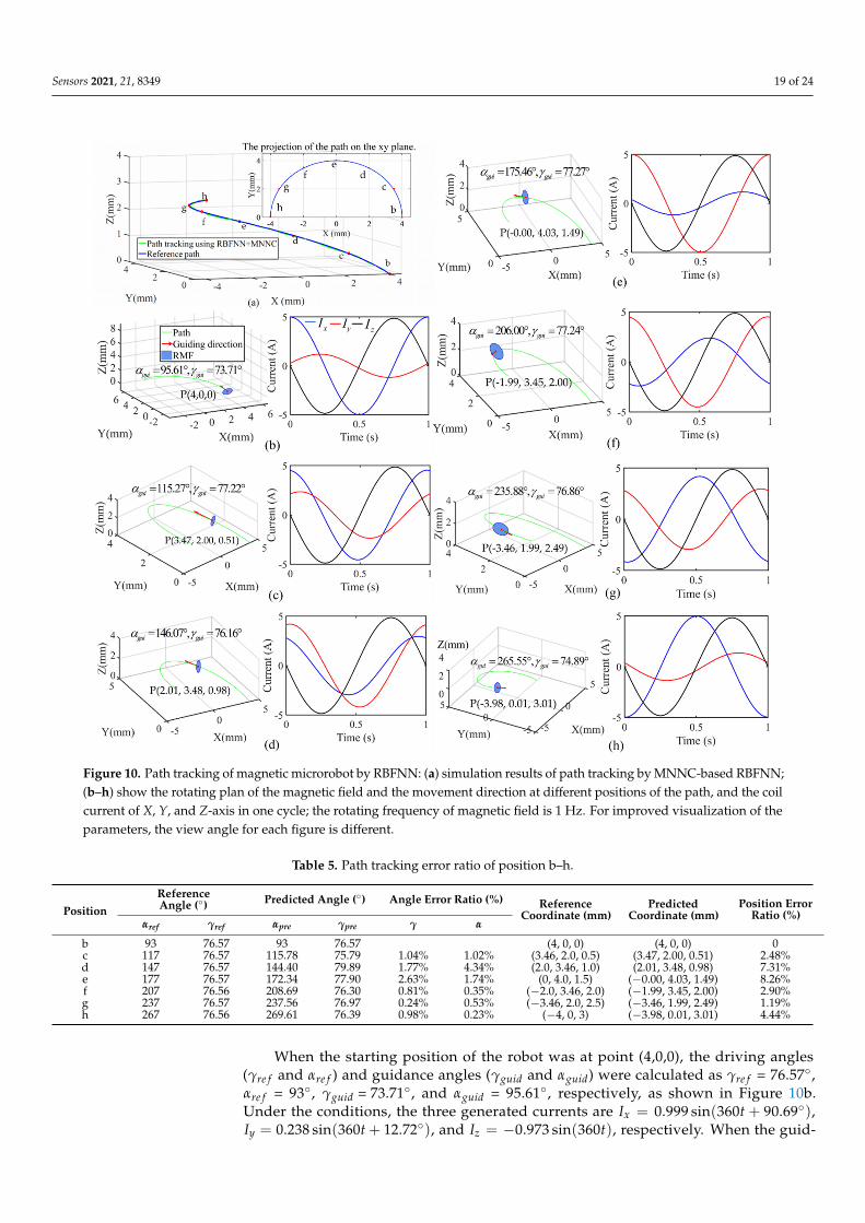
The simulation result of seven positions are shown in Table 5 and Figure 10.Because the control angles determine the steering direction, the two control angles

automatically generate three current signals to produce an RMF and determine the positionof the plane of RMF, as shown in Figure 10. Figure 10a shows the reference path andthe simulation result of the path tracking on the reference path using RBFNN along withMNNC. Figure 10b–h shows the seven positions of the robot and their control conditionsaccording to the changes in the control angles. There are the coordinates of position,reference path (green curve), plane of RMF (blue circle plan), movement direction (redarrow), or the direction of the normal vector of the plane of the rotating magnetic field, thecontrol angles, and the generated currents in one cycle of the three-axis Helmholtz coils. Atthe seven positions on the path, the generated current signals for the RMFs are summarizedin Table 4. We assumed that the frequency of RMF was 1 Hz and the coefficients µ0NKB ofthe coil were normalized as 1. In addition, the robot has a right-handed screw mechanism,and the rotating direction of the magnetic field is clockwise. In this case, the direction ofnormal vector becomes the movement direction of the robot, and the control angles becomethe steering direction of the robot.

Sensors 2021, 21, 8349 19 of 24Sensors 2021, 21, x FOR PEER REVIEW 21 of 27

Figure 10. Path tracking of magnetic microrobot by RBFNN: (a) simulation results of path tracking by MNNC-based RBFNN; (b–h) show the rotating plan of the magnetic field and the movement direction at different positions of the path, and the coil current of X, Y, and Z-axis in one cycle; the rotating frequency of magnetic field is 1 Hz. For improved visualization of the parameters, the view angle for each figure is different.

When the starting position of the robot was at point (4,0,0), the driving angles ( refγ

and refα) and guidance angles ( guidγ and guidα

) were calculated as refγ = 76.57°, refα

= 93°, guidγ = 73.71°, and guidα = 95.61°, respectively, as shown in Figure 10b. Under the

conditions, the three generated currents are 0.999sin(360 90.69 )xI t= + ° , 0.238sin(360 12.72 )yI t= + °

, and 0.973sin(360 )zI t= − , respectively. When the guidance

angles of guidγ and guidα are 77.22° and 115.27°, the robot reaches Position c, as shown

in Figure 10c. Moving from Position b to c, we can confirm that the current profiles are

changed by the variation of the guidance angles (steering angles). guidα allows the RMF

plane to rotate around the Z-axis and the changes in the guidγ cause the RMF plane to rotate around X-axis or Y-axis or both (Figure 7a). Therefore, when there is no angular change in the moving path of the robot, the generated current profiles are constant, while

Figure 10. Path tracking of magnetic microrobot by RBFNN: (a) simulation results of path tracking by MNNC-based RBFNN;(b–h) show the rotating plan of the magnetic field and the movement direction at different positions of the path, and the coilcurrent of X, Y, and Z-axis in one cycle; the rotating frequency of magnetic field is 1 Hz. For improved visualization of theparameters, the view angle for each figure is different.

Table 5. Path tracking error ratio of position b–h.

PositionReferenceAngle (◦) Predicted Angle (◦) Angle Error Ratio (%) Reference

Coordinate (mm)Predicted

Coordinate (mm)Position Error

Ratio (%)αref γref αpre γpre γ α

b 93 76.57 93 76.57 (4, 0, 0) (4, 0, 0) 0c 117 76.57 115.78 75.79 1.04% 1.02% (3.46, 2.0, 0.5) (3.47, 2.00, 0.51) 2.48%d 147 76.57 144.40 79.89 1.77% 4.34% (2.0, 3.46, 1.0) (2.01, 3.48, 0.98) 7.31%e 177 76.57 172.34 77.90 2.63% 1.74% (0, 4.0, 1.5) (−0.00, 4.03, 1.49) 8.26%f 207 76.56 208.69 76.30 0.81% 0.35% (−2.0, 3.46, 2.0) (−1.99, 3.45, 2.00) 2.90%g 237 76.57 237.56 76.97 0.24% 0.53% (−3.46, 2.0, 2.5) (−3.46, 1.99, 2.49) 1.19%h 267 76.56 269.61 76.39 0.98% 0.23% (−4, 0, 3) (−3.98, 0.01, 3.01) 4.44%

When the starting position of the robot was at point (4,0,0), the driving angles(γre f and αre f ) and guidance angles (γguid and αguid) were calculated as γre f = 76.57◦,αre f = 93◦, γguid = 73.71◦, and αguid = 95.61◦, respectively, as shown in Figure 10b.Under the conditions, the three generated currents are Ix = 0.999 sin(360t + 90.69◦),Iy = 0.238 sin(360t + 12.72◦), and Iz = −0.973 sin(360t), respectively. When the guid-

Sensors 2021, 21, 8349 20 of 24

ance angles of γguid and αguid are 77.22◦ and 115.27◦, the robot reaches Position c, asshown in Figure 10c. Moving from Position b to c, we can confirm that the currentprofiles are changed by the variation of the guidance angles (steering angles). αguidallows the RMF plane to rotate around the Z-axis and the changes in the γguid cause theRMF plane to rotate around X-axis or Y-axis or both (Figure 7a). Therefore, when thereis no angular change in the moving path of the robot, the generated current profilesare constant, while the current profiles are changed when there is an angular changein the moving path. Through the phase difference and amplitude of the currents, themovement direction of the robot is determined.

In Figure 10c, the present position of the microrobot is (3.47, 2.00, 0.51). The guidanceangle γguid and αguid are 77.22◦ and 115.27◦, respectively, that were obtained by RBFNN.The control system calculated the corresponding coils current along the x-axis, y-axis, andz-axis indicated by the blue, red, and green curves, respectively, as shown in Figure 10c.The amplitudes of Ix, Iy, and Iz are 0.909, 0.471, and 0.975, respectively, as shown in Table 4.From Table 4, we can observe that the phase of Ix, Iy, and Iz are 95.96◦, 64.89◦, and 0,respectively. Comparing Figure 10b,c the current in the z-axis coils of these two cases aresimilar because the angle γguid changes negligibly. However, there are large changes in thecurve corresponding to the current in the x-axis and y-axis coils because the angle αguidchanges significantly; therefore, we can obtain the results using Equations (24) and (25).The similar control process was implemented for the other positions, and the correspondingresults are shown in Figure 10c–g and Table 5. The error ratios of path tracking are shownin Table 5. When the microrobot is at Position c, the reference target position and actualposition coordinates are (3.5, 2.0, 0.5) and (3.47, 2.00, 0.51), respectively. We calculated thereference distance from the starting position to the reference target position for each step,and calculated the deviation between reference target and predicted position. Accordingly,the path tracking error ratios at Positions c, d, e, f, g, and h, are obtained as shown inTable 5. Because Position b is the initial position of the entire path tracking, there is no errorat this time. The error ratios are primarily less than 5%. Finally, the microrobot realized thelocomotion along the reference path as shown in Figure 10h. The standard deviation ofposition is 0.0145 mm. According to the result, we can conclude that the control systembased on RBFNN can provide the control direction of each position. Subsequently, thecorresponding coil currents can be calculated to generate the rotating magnetic field fordriving the robot to move along the reference direction.

In the actual experiment, it is necessary to obtain some training samples for RBFNNlearning, to establish the relationship between the reference angle and control angle. First,we can obtain the present position P0 of robot. We set the control direction with angle γcontand αcont, and calculate the currents of the Helmholtz coils. Thereafter, the Helmholtz coilsgenerate the rotating magnetic field and drive the spring-type robot to the position Pre f . Thesimulation result for this case shows that if we want to drive the robot from P0 to Pre f , we canset the control angle γcont and αcont to generate a rotating magnetic field for the movementof the robot. The direction from P0 to Pre f is the reference direction. We can calculate theangle γre f and αre f of the direction from P0 to Pre f using Equations (31) and (32). Thus, atraining sample with components of γre f ,αre f , γcont, and αcont is obtained. In this manner,we can obtain many training samples and train the RBFNN.

After the RBFNN is trained, we can apply the control system based on RBFNN to pathtracking control. We can obtain the reference target position and present position of eachstep, and subsequently calculate the reference angle γre f and αre f to provide as input tothe RBFNN. RBFNN outputs the control angle γcont and αcont. Next, the control systemcan derive the current of Helmholtz coils, and subsequently generate the RMF to drive therobot to the reference target position.

6. Discussion

Clustering algorithms can classify similar samples into the same cluster, but theconventional clustering algorithms often require the determination of several important pa-

Sensors 2021, 21, 8349 21 of 24

rameters based on experience in advance, thus leading to inconvenience. Moreover, whenconventional clustering algorithms are applied in some specific situations, the clusteringalgorithms can be improved to increase efficiency and accuracy. MNNC determines thesamples with the highest similarity based on the determination of the nearest neighbors.Because the data of curve fitting and path following control have the characteristics ofobvious time or spatial sequence, the performance of the MNNC is considerably improvedfor this type of data. MNNC reduces the range of determining the nearest neighbor thatreduces the computation cost, thereby requiring few parameters to be set. Furthermore,it can adaptively adjust the number of clusters. Moreover, MNNC can determine theabnormal samples in the dataset and adjust them. After the adjusted data is used for curvefitting, the fitting accuracy can be improved by 50%; particularly, the adjustment effect ismore prominent when there are not many outliers because the adjustment is performed onthe samples with the largest outliers, and the sample adjustment is a gradual process. Theabnormal sample adjustment of MNNC can avoid misjudgment and over-adjustment ofoutliers. For cases with a large number of outliers, the adjustment effect can be enhancedby increasing the number of optimizations.

RBFNN is commonly used in nonlinear systems for curve fitting and path trackingcontrol. Using a clustering algorithm to obtain the initial parameters of RBFNN is a rela-tively simple method. When MNNC is used to train RBFNN, the number of hidden nodesof RBFNN can be changed by automatically adjusting the number of clusters according tothe accuracy requirements of RBFNN, to improve the accuracy of RBFNN. The simulationresults show that the curve fitting accuracy of RBFNN trained by MNNC is up to 60%higher than that of other RBFNNs.

When the magnetic microrobot is moving, it is difficult to reach the target positionaccurately due to the interference of various factors. In this study, the motion mechanismof the magnetic robot is analyzed, and a locomotion control system based on RBFNN isproposed. The system uses RBFNN to determine the reference target of the theoreticallocomotion target, and controls the magnetic microrobot to reach the theoretical motiontarget by moving to the reference target. In order to use MNNC to establish the parametersof RBFNN better, this study enhanced the function of MNNC on the basis of the previousanalysis. The simulation results show that the enhanced MNNC demonstrates an improvedperformance over traditional clustering algorithms in clustering analysis, and there arefewer parameters to be determined in advance. The simulation results show that a bettercontrol effect can be obtained after applying RBFNN based on MNNC in the path trackingcontrol of the magnetic robot.

Although MNNC has only been applied in clustering 2D data in this study, it can adaptto multidimensional datasets. This will be verified in future research, and the algorithmwill be improved to increase the clustering accuracy and generalization ability.

7. Conclusions

A modified nearest neighbor-based clustering algorithm is proposed in this study thatdoes not necessitate the setting of important parameters relying on past experience, andcan perform cluster analysis on samples of different densities and shapes. The abnormalsamples can be found, and the adjustment of the sample can be realized by this clusteringalgorithm. The simulation results show that the curve fitting accuracy of the samplesoptimized by the clustering algorithm is increased by 50%. The number and center of basisfunctions can be automatically determined by applying this clustering algorithm on thetraining samples of RBFNN. The simulation results proved that the RBFNN trained in thismanner has a higher operating accuracy than the conventional RBFNN; the accuracy incurve fitting is improved by 60%. The simulation result showed that the RBFNN basedon the clustering algorithm could improve the accuracy in the path tracking simulationby 20%.

Sensors 2021, 21, 8349 22 of 24

Author Contributions: Conceptualization, D.Z. and S.K.; methodology, D.Z.; validation, W.J. andS.K.; investigation, D.Z.; writing—original draft preparation, D.Z.; writing—review and editing,W.J. and S.K.; supervision, S.K. All authors have read and agreed to the published version ofthe manuscript.

Funding: This work was supported in part by the Korea Medical Device Development Fund grantfunded by the Korea government (the Ministry of Science and ICT, the Ministry of Trade, Indus-try and Energy, the Ministry of Health & Welfare, the Ministry of Food and Drug Safety) (ProjectNumber: KMDF_PR_20200901_0130, 9991006803), and in part by the National Research Founda-tion of Korea (NRF) grant funded by the Korea government (MSIT) (No. 2020R1A4A3079595 and2018R1C1B6003491).

Institutional Review Board Statement: Not applicable.

Informed Consent Statement: Not applicable.

Data Availability Statement: Data can be requested from the corresponding authors.

Conflicts of Interest: The authors declare no conflict of interest.

Appendix A

Table A1. List of acronyms.

RBFNN Radial basis function neural networkMNNC Modified nearest neighbor-based clusteringPID Proportion integral differentialSVM Support vector machinesGA Genetic algorithmAI Artificial immuneDBSCAN Density-based spatial clustering of applications with noiseDPC Density peaks clusteringACC AccuracyADI Adjusted Rand indexRMF Rotating magnetic fieldBIRCH Balanced iterative reducing and clustering using hierarchiesCLIQUE Clustering in QUEst

Appendix B

Table A2. List of variables.

di Distance between sample and its nearest neighborH The number of di levelPi Sample∆D Distance changedstep Distance stepD Total distances between samples and centroid of cluster before mergedD’ Total distances between samples and centroid of cluster after mergedQuani Quantity of samples of cluster iC Center of clusterR Scanning radius of DBSCANTm Magnetic torqueV Volume of microrobotM Magnetization of microrobotB External magnetic fieldγ Polar angleα Azimuthal angle

Sensors 2021, 21, 8349 23 of 24

Table A2. Cont.

nB Normal vector of plan PPcont Control positionPref Reference positionPact Actual positionPguid Guidance positionPpre Predicted positionγref Reference polar angleαref Reference azimuthal angleγcont Control polar angleαcont Control azimuthal angleγguid Guidance polar angleαguid Guidance azimuthal angleγpre Predicted polar angleαpre Predicted azimuthal angleγcomp Compensation of polar angleαcomp Compensation of azimuthal angledcont Control directiondguid Guidance directiondref Reference directiondpre Predicted directiondact Actual directionQi Output of hidden layer neuron of RBFNNci Center of hidden layer neuron of RBFNNwi Weight between hidden layer and output layer of RBFNNσ Width of hidden layer neuron of RBFNNµ0 Permeability of free spaceN Turns number of coilKB Magnetic field coefficient of Helmholtz coilI Coil currentIx Coil current of x-axisIy Coil current of y-axisIz Coil current of z-axiserrgamma Error of polar angleerralpha Error of azimuthal angleerrposition Error of position

References1. Rout, R.; Subudhi, B. Inverse optimal self-tuning PID control design for an autonomous underwater vehicle. Int. J. Syst. Sci. 2017,

48, 367–375. [CrossRef]2. Xiang, H.B.; Li, M.W.; Zhang, T.L.; Wang, S.J.; Zhang, M.; Song, Y.; Huo, W.X.; Huang, X. Motion characteristics of untethered

swimmer with magnetoelastic material. Smart Mater. Struct. 2021, 30, 075030. [CrossRef]3. Ghosh, B.B.; Sarkar, B.K.; Saha, R. Realtime performance analysis of different combinations of fuzzy-PID and bias controllers for a

two degree of freedom electrohydraulic parallel manipulator. Robot. Comput.-Integr. Manuf. 2015, 34, 62–69. [CrossRef]4. Algarin-Pinto, J.A.; Garza-Castanon, L.E.; Vargas-Martinez, A.; Minchala-Avila, L.I. Dynamic modeling and control of a parallel

mechanism used in the propulsion system of a biomimetic underwater vehicle. Appl. Sci. 2021, 11, 4909. [CrossRef]5. Mai, T.A.; Dang, T.S.; Duong, D.T.; Le, V.C.; Banerjee, S. A combined backstepping and adaptive fuzzy PID approach for trajectory

tracking of autonomous mobile robots. J. Braz. Soc. Mech. Sci. Eng. 2021, 43, 156. [CrossRef]6. Xu, B.J.; Ji, S.; Zhang, C.R.; Chen, C.; Ni, H.P.; Wu, X.J. Linear-extended-state-observer-based prescribed performance control for

trajectory tracking of a robotic manipulator. Ind. Robot. 2021, 44, 544–555. [CrossRef]7. Li, Q.X.; Zhou, Y.S. Precise trajectory tracking control of ship towing systems via a dynamical tracking target. Mathematics 2021, 9,

974. [CrossRef]8. Wu, Y.; Wang, L.; Zhang, J.; Li, F. Path following control of autonomous ground vehicle based on nonsingular terminal sliding

mode and active disturbance rejection control. IEEE Trans. Veh. Technol. 2019, 68, 6379–6390. [CrossRef]9. Liu, C.; Cheah, C.C.; Slotine, J. Adaptive Jacobian PID regulation for robots with uncertain kinematics and actuator model. In

Proceedings of the 2006 IEEE/RSJ International Conference on Intelligent Robots and Systems, Beijing, China, 9–15 October 2006;pp. 3044–3049. [CrossRef]

10. Smeresky, B.; Rizzo, A.; Sands, T. Optimal learning and self-awareness versus PDI. Algorithms 2020, 13, 23. [CrossRef]11. Juang, J.G. Intelligent trajectory control using recurrent averaging learning. Appl. Artif. Intell. 2001, 15, 277–296. [CrossRef]

Sensors 2021, 21, 8349 24 of 24

12. Chen, Z.; Yang, X.; Liu, X. RBFNN-based nonsingular fast terminal sliding mode control for robotic manipulators includingactuator dynamics. Neurocomputing 2019, 362, 72–82. [CrossRef]

13. Nie, L.; Guan, J.; Lu, C. Longitudinal speed control of autonomous vehicle based on a self-adaptive PID of radial basis functionneural network. IET Intell. Transp. Syst. 2018, 12, 485–494. [CrossRef]

14. Lee, C.T.; Tsai, C.C. Improved nonlinear trajectory tracking using RBFNN for a robotic helicopter. Int. J. Robust Nonlinear Control2010, 20, 1079–1096. [CrossRef]

15. Li, J.; Wang, J.; Wang, S. Neural approximation-based model predictive tracking control of non-holonomic wheel-legged robots.Int. J. Control Autom. Syst. 2020, 19, 372–381. [CrossRef]

16. Guillen, A.; Rojas, I.; Gonzalez, J. Output value-based initialization for radial basis function neural networks. Neural Process. Lett.2007, 25, 209–225. [CrossRef]

17. Juang, J.G. Effects of Using Different Neural Network Structures and Cost Functions in Locomotion Control. In Lecture Notes inComputer Science, Proceedings of the 2nd International Conference on Natural Computation (ICNC 2006), Xian, China, 24–28, September2006; Springer: Berlin/Heidelberg, Germany, 2006. [CrossRef]

18. Fernandez-Navarro, F.; Hervas-Martinez, C.; Gutierrez, P.A. Generalised gaussian radial basis function neural networks. SoftComput. 2013, 17, 519–533. [CrossRef]

19. Huang, H.C.; Chiang, C.H. An evolutionary radial basis function neural network with robust genetic-based immunecomputingfor online tracking control of autonomous Robots. Neural Process. Lett. 2016, 44, 19–35. [CrossRef]

20. Chen, Z.Y.; Kuo, R.J. Combining SOM and evolutionary computation algorithms for RBF neural network training. J. Intell. Manuf.2019, 30, 1137–1154. [CrossRef]

21. Guillén, A.; Rojas, I.; Gonzalez, J. A possibilistic approach to RBFN centers initialization. In Lecture Notes in Computer Science,Proceedings of the 10th International Conference on Rough Sets, Fuzzy Sets, Data Mining and Granular Computing (RSFDGrC 2005),Regina, SK, Canada, 31 August 2005; Springer: Berlin/Heidelberg, Germany, 2005. [CrossRef]

22. Oh, S.K.; Kim, W.D.; Pedrycz, W. Design of k-means clustering-based polynomial radial basis function neural networks (pRBF-NNs) realized with the aid of particle swarm optimization and differential evolution. Neurocomputing 2012, 78, 121–132. [CrossRef]

23. Liao, C.C. Genetic k-means algorithm based RBF network for photovoltaic MPP prediction. Energy 2010, 35, 529–536. [CrossRef]24. Dogan, A.; Birant, D. Machine learning and data mining in manufacturing. Expert Syst. Appl. 2021, 166, 114060. [CrossRef]25. Fan, Y.K.; Bai, J.R.; Lei, X.; Lin, W.G.; Hu, Q.; Wu, G.D.; Guo, J.M.; Tan, G. PPMCK: Privacy-preserving multi-party computing for

K-means clustering. J. Parallel Distrib. Comput. 2020, 154, 54–63. [CrossRef]26. Khalid, A.; Hammed, A. Genetic divergence in wheat genotypes based on seed biochemical profiles appraised through agglomer-

ative hierarchical clustering and association analysis among traits. Pak. J. Bot. 2021, 53, 1281–1286. [CrossRef]27. Fang, X.J.; Wu, Y.J.; Liao, S.S.; Xue, L.Z.; Chen, Z.; Yang, J.N.; Lu, Y.M.; Ling, K.; Hu, S.Y.; Kong, S.Y. Division of crustal units in

China using grid-based clustering and a zircon U-Pb geochronology database. Comput. Geosci. 2020, 145, 104570. [CrossRef]28. Montanari, G.E.; Doretti, M.; Marino, M.F. Model-based two-way clustering of second-level units in ordinal multilevel latent

Markov models. Adv. Data Anal. Classif. 2021, 1–29. [CrossRef]29. Luo, S.; Liu, H.W.; Qi, E. Recognition and labeling of faults in wind turbines with a density-based clustering algorithm. Data

Technol. Appl. 2021. [CrossRef]30. Li, C.Z.; Zhang, Y.Z. Density peak clustering based on relative density optimization. Math. Probl. Eng. 2020, 2020, 2816102.

[CrossRef]31. Syarrudin, M.; Alfian, G.; Fitriyani, N.L. Performance analysis of IoT-based sensor, big data processing, and machine learning

model for real-time monitoring system in automotive manufacturing. Sensors 2018, 18, 2946. [CrossRef]32. Minimol, P.V.; Mishra, D.; Gorthi, R.K.S.S. Guided MDNet tracker with guided samples. Visual Comput. 2021, 1–15. [CrossRef]33. Jeon, S.; Kim, S.; Ha, S.; Lee, S.; Kim, E.; Kim, S.Y.; Park, S.H.; Jeon, J.H.; Kim, S.W.; Moon, C. Magnetically actuated microrobots

as a platform for stem cell transplantation. Sci. Robot. 2019, 4, eaav4317. [CrossRef]34. Chen, X.Z.; Hoop, M.; Mushtaq, S.F.; Hu, E.C.Z.; Nelson, B.J.; Pane, S. Recent developments in magnetically driven micro- and

nanorobots. Appl. Mater. Today 2017, 9, 37–46. [CrossRef]35. Li, J.; Li, X. Development of a magnetic microrobot for carrying and delivering targeted cells. Sci. Robot. 2018, 3, eaat8829.

[CrossRef] [PubMed]36. Yan, X.H.; Zhou, Q.; Vincent, M.; Deng, Y.; Yu, J.F.; Xu, J.B.; Xu, T.T.; Tang, T.; Bian, L.M.; Wang, Y.X.J.; et al. Multifunctional

biohybrid magnetite microrobots for imaging-guided therapy. Sci. Robot. 2017, 2, eaaq1155. [CrossRef] [PubMed]37. Yang, C.; Wang, X.; Cheng, L. Neural-learning-based telerobot control with guaranteed performance. IEEE Trans. Cybern. 2017, 47,

3148–3159. [CrossRef] [PubMed]