Journal of Statistical Planning andInference 76 (1999) 163–183

Classi�cation of multiple observations using multi-stagerank nearest neighbor rule

S.C. Bagui a; ∗, K.L. Mehra ba Department of Mathematics and Statistics, The University of West Florida, Pensacola,

FL 32514, USAb Department of Mathematical Sciences, University of Alberta, Edmonton, AB, Canada T6G 2G1

Received 11 April 1997; accepted 9 June 1998

Abstract

In this article, a multi-stage (M -stage) rank nearest-neighbor (MRNN)-type rule is proposedand studied for the classi�cation of a sample of multiple (m) independent univariate observationsbetween two populations. The asymptotic total probability of misclassi�cation (TPMC) – viz.,the asymptotic risk R(M)(m) – for the proposed MRNN rule is derived. It is shown �rstly that (i)the asymptotic risk R(1)(2) of the 1st stage RNN rule for m=2 is lower than the correspondingrisk R(1)(1) for m=1, by a factor less than one, and secondly that (ii) for m=2, the M -stage ruleasymptotic risk R(M)(2) decreases as the number M of the stages employed increases. The formerresult leads to an improved upper bound on R(1)(2) in terms of Bayes risk R∗(1) (cf. Cover andHart (1967) IEEE Trans. Inform. Theory, Das Gupta and Lin (1980) Sankhya A). Also, a cross-validation-type estimator for the asymptotic risk R(1)(m) is shown to be asymptotically unbiasedand L2-consistent. Finally, some comparative Monte-Carlo results are reported to illuminate theperformance characteristics of the proposed rule in small sample situations. c© 1999 ElsevierScience B.V. All rights reserved.

AMS classi�cations: primary 62H30; secondary 62G10; 62F15; 62G20

Keywords: Multiple measurement classi�cation; Rank nearest neighbor classi�cation; Multiplemeasurement discrimination

1. Introduction

1.1. The classi�cation problem

In many practical situations, multiple measurements are frequently taken on individ-uals awaiting classi�cation. In a medical context, a patient may be recalled for furtherrepeated measurements of the same variable with the intent of providing a �rmer basisfor diagnosis of his or her condition. In diagnosing hypertension, the blood pressure of

∗ Corresponding author. Tel.: +1 850 474 2286; fax: +1 850 474 3131; e-mail: sbagui@uwf.edu.

0378-3758/99/$ – see front matter c© 1999 Elsevier Science B.V. All rights reserved.PII: S0378 -3758(98)00137 -2

164 S.C. Bagui, K.L. Mehra / Journal of Statistical Planning and Inference 76 (1999) 163–183

a patient is often measured repeatedly over weeks or months before making any deci-sion on a speci�c therapy (see McLachlan, 1992). Choi (1972) considered an examplein which multiple measurements on vascular basement membrane (BM) thickeningin body capillaries were used to classify individual patients as normal or diabetic.This article proposes and studies a nonparametric multi-stage rank nearest-neighbor(MRNN)-type rule for the classi�cation of samples consisting of m multiple univariatei.i.d. observations.A nearest-neighbor (NN)-type classi�cation rule was �rst introduced by Fix and

Hodges (1951). Their proposed k-NN rule for two populations is described as fol-lows: Suppose an unknown observation Z known to originate from one of two distinctpopulation �1 and �2 is to be correctly classi�ed into its parent population. The onlyinformation available is in the form of independent ‘training’ samples {X1; X2; : : : ; Xn}and {Y1; Y2; : : : ; Yn}, respectively, of i.i.d. observations from �1 and �2. Using a distancefunction and a �xed integer k¿0, the k-NN rule assigns Z to �1 if k1=n1¿k1=n2, whereki=# of observations from �i (i=1; 2) among k = k1 + k2 observations nearest to Z .Cover and Hart (1967) considered a slightly modi�ed version of the above k-NN rulewhich assigns Z to �i if ki=max{k1; k2}. They showed that for their 1-NN rule, thelimiting error rate R(1) has bounds R∗(1)6R(1)6 2R∗(1)(1−R∗(1)), where R∗(1) isthe (minimum) Bayes error rate (see Eq. (2.18) below). Other aspects of this problemhave been studied, among others, by Wagner (1971), Fritz (1975), Devroye (1981)and Xiru (1985). However, as the important reference by Fix and Hodges (1951) israther inaccessible, it could be pointed out that this paper has been reprinted at theend of the commentary on it by Silverman and Jones (1989). Anderson (1966) hadearlier suggested a nonparametric classi�cation rule for univariate populations basedon ranks, which was subsequently studied by Das Gupta and Lin (1980). Das Guptaand Lin named this procedure the RNN rule. Their 1-RNN rule may be described asfollows: Pool the observations, Xi’s, Yj’s and Z , and rank them in ascending order; (i)if both the immediate rank neighbors of Z belong to same population, classify Z to thatpopulation; (ii) if Z is either the smallest or largest in the pool sample, classify Z intothe population of its rank nearest neighbor; (iii) if the immediate left and right rankneighbors of Z belong to two di�erent populations, classify Z into either of the twopopulations with probability 1

2 each (to break the tie). They derived the asymptotic riskof the above 1-RNN rule which turned out to be exactly the same as derived by Coverand Hart for their 1-NN rule. Very recently, Bagui and Vaughn (1998) proposed andstudied the asymptotic properties the k-RNN rule. They obtained suitable bounds forthe asymptotic risk and also showed that the asymptotic risk is Bayes risk consistent,and it decreases as the value of k increases. For other aspects of the k-RNN rule seeBagui et al. (1997).Besides Choi (1972), the problem of classi�cation of multiple observations in para-

metric situations have been studied, among others, by Gupta (1986), and Gupta andLogan (1990). These authors considered a two factor mixed hierarchical univariatemodel under normality assumptions. Choi (1972) derived the optimal Bayes classi�-cation rule; Gupta (1986) obtained expressions for the rates of the Bayes rule. The

S.C. Bagui, K.L. Mehra / Journal of Statistical Planning and Inference 76 (1999) 163–183 165

multivariate case was studied recently by Gupta and Logan (1990) under multivariatenormality assumptions. In the nonparametric case also, there have been several attemptsat providing suitable classi�cation rules for multiple observations, under varying as-sumptions of location shifts, scale di�erences or stochastic orderings among populations.While Das Gupta (1964) and Hudimoto (1964) based their rules on the Kolmogorovdistance and Wilcoxon statistics, Lin (1979) employed generalized U-statistics (andLehmann statistic, in particular) and Govindarajulu and Gupta (1977) used Cherno�–Savage linear rank-statistics for their classi�cation procedures. In view of the ‘consis-tency’ results proved in the respective papers, these procedures all seem appropriatewhen both size m of the sample to be classi�ed and the sizes n1 and n2 of the trainingsamples are su�ciently large. On the other hand, in practical situation m is usually �xedand small and only the training sample sizes n1 and n2 may be assumed to increaseinde�nitely. In this article, we propose a left–right multi-stage rank nearest-neighborclassi�cation rule for �xed m and study its properties under latter situation. Recently,Bagui (1993) and Bagui et al. (1995) considered the problem of classi�cation of i.i.d.multiple observations between populations. Bagui (1993) used a distance NN-type ruleand obtained the asymptotic risk of the proposed rule. Bagui et al. (1995) proposed adi�erent type of distance NN rule that classi�es a set of i.i.d. multiple by subgroupingthe training samples. They showed that the asymptotic risk of the proposed rule hasthe bounds for general m that are counter-part of those in Cover and Hart (1967) form=1. The present work generalizes the work of Das Gupta and Lin (1980) from oneto m observations. It is a majority vote rule that uses 1-RNN as described by Das Guptaand Lin (1980) for each multiple observations to be classi�ed. It will be even moreinteresting to study a majority vote rule that will make use of k-RNN as described byBagui et al. (1997) in classifying i.i.d. multiple observations.

1.2. The proposed MRNN classi�cation rules

Suppose {X1; X2; : : : ; Xn1} and {Y1; Y2; : : : ; Yn2} represent independent ‘training’ sam-ples of i.i.d. observations from the two univariate populations �1 and �2, respectively.Suppose further that {Z1; Z2; : : : ; Zm} is a sample of i.i.d. observations from either �1 or�2, and is to be correctly classi�ed into its parent population by utilizing the informa-tion contained in the two preceding ‘training’ samples. We now describe our 1st-stagerank nearest-neighbor classi�cation rule as follows: Combine Xi’s, Yj’s and Zl’s, andarrange them in increasing order, identifying the �rst left- and right-hand rank nearestneighbors of each Zl for l=1; 2; : : : ; m. Then the 1st-stage RNN rule is:

Classify Z into �1; with probability 1;if # (1st-stage) RNNs from �1¿ if # (1st-stage) RNNs from �2:

Classify Z into �2; with probability 1;if # (1st-stage) RNNs from �1¡ if # (1st-stage) RNNs from �2:

Classify Z into �1 or �2; with probability 12 each (to break the tie);

if # (1st-stage) RNNs from �1 = if # (1st-stage) RNNs from �2;

(1.1)

where Z = {Z1; Z2; : : : ; Zm}.

166 S.C. Bagui, K.L. Mehra / Journal of Statistical Planning and Inference 76 (1999) 163–183

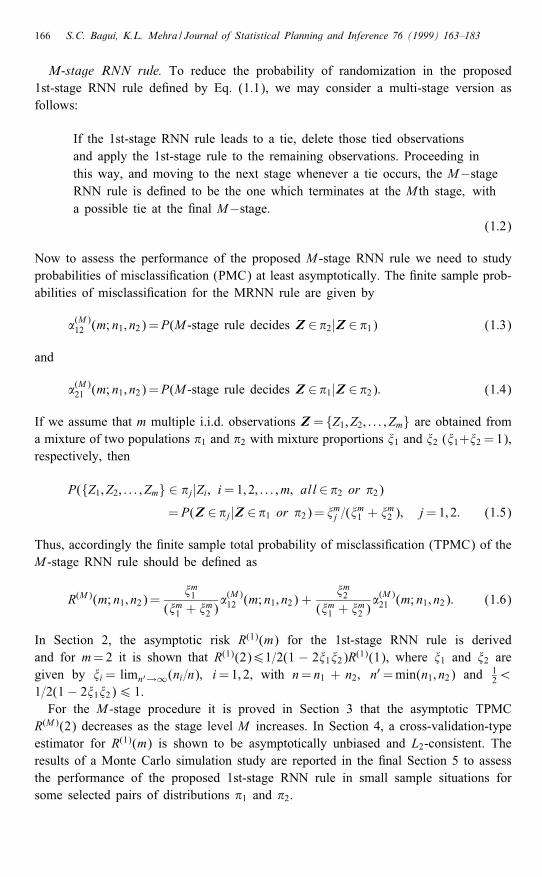
M-stage RNN rule. To reduce the probability of randomization in the proposed1st-stage RNN rule de�ned by Eq. (1.1), we may consider a multi-stage version asfollows:

If the 1st-stage RNN rule leads to a tie, delete those tied observationsand apply the 1st-stage rule to the remaining observations. Proceeding inthis way, and moving to the next stage whenever a tie occurs, the M−stageRNN rule is de�ned to be the one which terminates at the M th stage; witha possible tie at the �nal M−stage:

(1.2)

Now to assess the performance of the proposed M -stage RNN rule we need to studyprobabilities of misclassi�cation (PMC) at least asymptotically. The �nite sample prob-abilities of misclassi�cation for the MRNN rule are given by

�(M)12 (m; n1; n2)=P(M -stage rule decides Z ∈ �2|Z ∈ �1) (1.3)

and

�(M)21 (m; n1; n2)=P(M -stage rule decides Z ∈ �1|Z ∈ �2): (1.4)

If we assume that m multiple i.i.d. observations Z = {Z1; Z2; : : : ; Zm} are obtained froma mixture of two populations �1 and �2 with mixture proportions �1 and �2 (�1+�2 = 1),respectively, then

P({Z1; Z2; : : : ; Zm} ∈ �j|Zi; i=1; 2; : : : ; m; all∈ �2 or �2)= P(Z ∈ �j|Z ∈ �1 or �2)= �mj =(�m1 + �m2 ); j=1; 2: (1.5)

Thus, accordingly the �nite sample total probability of misclassi�cation (TPMC) of theM -stage RNN rule should be de�ned as

R(M)(m; n1; n2)=�m1

(�m1 + �m2 )�(M)12 (m; n1; n2) +

�m2(�m1 + �

m2 )�(M)21 (m; n1; n2): (1.6)

In Section 2, the asymptotic risk R(1)(m) for the 1st-stage RNN rule is derivedand for m=2 it is shown that R(1)(2)61=2(1 − 2�1�2)R(1)(1), where �1 and �2 aregiven by �i= limn′→∞(ni=n); i=1; 2, with n= n1 + n2; n′=min(n1; n2) and 1

2¡1=2(1− 2�1�2)6 1.For the M -stage procedure it is proved in Section 3 that the asymptotic TPMC

R(M)(2) decreases as the stage level M increases. In Section 4, a cross-validation-typeestimator for R(1)(m) is shown to be asymptotically unbiased and L2-consistent. Theresults of a Monte Carlo simulation study are reported in the �nal Section 5 to assessthe performance of the proposed 1st-stage RNN rule in small sample situations forsome selected pairs of distributions �1 and �2.

S.C. Bagui, K.L. Mehra / Journal of Statistical Planning and Inference 76 (1999) 163–183 167

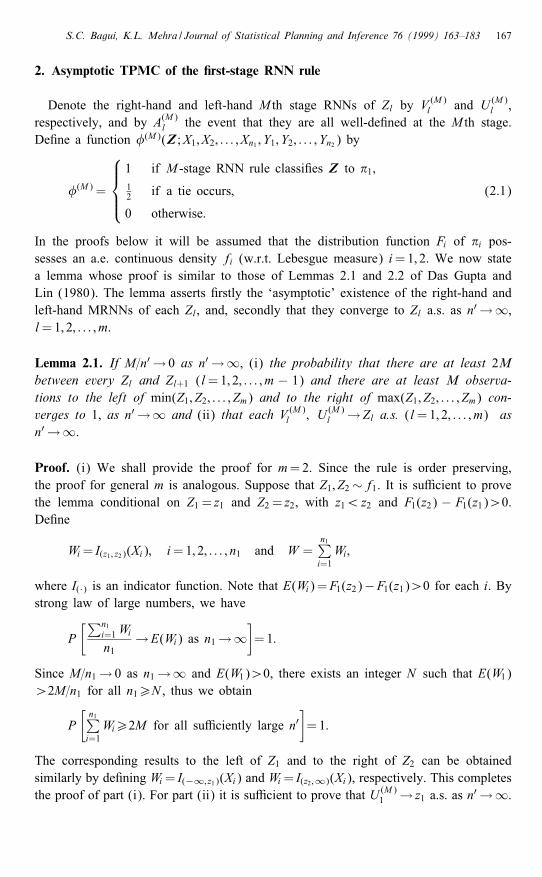
2. Asymptotic TPMC of the �rst-stage RNN rule

Denote the right-hand and left-hand M th stage RNNs of Zl by V(M)l and U (M)

l ,respectively, and by A(M)l the event that they are all well-de�ned at the M th stage.De�ne a function �(M)(Z ;X1; X2; : : : ; Xn1 ; Y1; Y2; : : : ; Yn2 ) by

�(M) =

1 if M -stage RNN rule classi�es Z to �1;12 if a tie occurs;

0 otherwise:

(2.1)

In the proofs below it will be assumed that the distribution function Fi of �i pos-sesses an a.e. continuous density fi (w.r.t. Lebesgue measure) i=1; 2. We now statea lemma whose proof is similar to those of Lemmas 2.1 and 2.2 of Das Gupta andLin (1980). The lemma asserts �rstly the ‘asymptotic’ existence of the right-hand andleft-hand MRNNs of each Zl, and, secondly that they converge to Zl a.s. as n′ →∞,l=1; 2; : : : ; m.

Lemma 2.1. If M=n′ → 0 as n′ →∞, (i) the probability that there are at least 2Mbetween every Zl and Zl+1 (l=1; 2; : : : ; m − 1) and there are at least M observa-tions to the left of min(Z1; Z2; : : : ; Zm) and to the right of max(Z1; Z2; : : : ; Zm) con-verges to 1, as n′ →∞ and (ii) that each V (M)l ; U (M)

l →Zl a.s. (l=1; 2; : : : ; m) asn′ →∞.

Proof. (i) We shall provide the proof for m=2. Since the rule is order preserving,the proof for general m is analogous. Suppose that Z1; Z2∼f1. It is su�cient to provethe lemma conditional on Z1 = z1 and Z2 = z2, with z1¡z2 and F1(z2) − F1(z1)¿0.De�ne

Wi= I(z1 ; z2)(Xi); i=1; 2; : : : ; n1 and W =n1∑i=1Wi;

where I(·) is an indicator function. Note that E(Wi)=F1(z2)−F1(z1)¿0 for each i. Bystrong law of large numbers, we have

P[∑n1

i=1Win1

→E(Wi) as n1→∞]=1:

Since M=n1→ 0 as n1→∞ and E(W1)¿0, there exists an integer N such that E(W1)¿2M=n1 for all n1¿N , thus we obtain

P[n1∑i=1Wi¿2M for all su�ciently large n′

]=1:

The corresponding results to the left of Z1 and to the right of Z2 can be obtainedsimilarly by de�ning Wi= I(−∞; z1)(Xi) and Wi= I(z2 ;∞)(Xi), respectively. This completesthe proof of part (i). For part (ii) it is su�cient to prove that U (M)

1 → z1 a.s. as n′ →∞.

168 S.C. Bagui, K.L. Mehra / Journal of Statistical Planning and Inference 76 (1999) 163–183

Note that for �¿0 and for almost all given Z1 = z1, {U (M)1 ¡z1− �}⊂{W¡M}, where

W is de�ned as above with (z1; z2) replaced by (z1 − �; z1), which implies

P(U (M)1 ¡z1 − �)6P(W¡M):

Now using Hoe�ding’s inequality for the sums of independent random variables (seeHoe�ding, 1963, pp. 15) we obtain the desired result.

2.1. Classi�cation of m=2 observations

We �rst obtain the TPMC of the 1st stage RNN classi�cation procedure. For thiswe will make use of conditioning techniques. The conditional probability, given Z = zof deciding z=(z1; z2) comes from �1 using the 1st-stage RNN procedure is given by

�(1)1 (z1; z2; n1; n2) = E(�(1)|Z1 = z1; Z2 = z2)

= E(�(1)I(A(1)1 ∩ A(1)2 )|Z1 = z1; Z2 = z2)

+E(�(1)I(A(1)1 ∩ A(1)2 )c|Z1 = z1; Z2 = z2); (2.2)

where in Eq. (2.2) I(:) stands for indicator function and the second expectation term

E(�(1)I(A(1)1 ∩ A(1)2 )c|Z1 = z1; Z2 = z2)6 P(A(1)

c

1 |Z1 = z1) + P(A(1)c

2 |Z2 = z2)

→ 0; as n′ →∞; (2.3)

the last convergence in Eq. (2.3) holding since by Lemma 2.1(i), the event that anyof the 1st-stage RNNs of Zl (l=1; 2) do not exist asymptotically is impossible. Indealing with the �rst expectation in Eq. (2.2), we need to consider a total of fourleft and right 1st-stage RNNs. The possibilities are that all four, any three, or anytwo 1st-stage RNNs could be from one population. Keeping this in mind and recallingde�nition (1.1) the �rst expectation in Eq. (2.2) can be written as

P[(�(1) = 1)∩A(1)1 ∩A(1)2 |Z = z] + 12P[(�

(1) = 12)∩A(1)1 ∩A(1)2 |Z = z]

= E

( ∑k=4;3

P(k;4−k)(U (1)1 ; V (1)1 ; U (1)

2 ; V (1)2 ; z1; z2)

)

+ 12 E(P

(2;2)(U (1)1 ; V (1)1 ; U (1)

2 ; V (1)2 ; z1; z2)): (2.4)

We note that

P(k;4−k)(u1; v1; u2; v2; z1; z2)=Ck(n1; n2; z1; z2)=B(n1; n2; z1; z2) (2.5)

S.C. Bagui, K.L. Mehra / Journal of Statistical Planning and Inference 76 (1999) 163–183 169

where for k =0; 1; 2; 3; 4;

Ck(n1; n2; z1; z2) = (n1Pk)(n2P4−k)(1− (Q(1)1 + Q(2)2 ))n1−k

×(1− (Q(1)1 + Q(2)2 ))n2−(4−k)

× ∑′{r1 ; r2 ; r3 ; r4}

fr1 (u1)fr2 (v1)fr3 (u2)fr4 (v2); (2.6)

Q( j)i =Fi(vj)− Fi(uj) for i=1; 2; j=1; 2;

and

B(n1; n2; z1; z2)=4∑k=0Ck(n1; n2; z1; z2): (2.7)

Note that Ck(n1; n2; z1; z2); k =0; 1; 2; 3; 4, are proportional to the conditional probabilitythat any k of the 4 RNNs comes from �1 and remaining (4 − k) comes from �2. InEq. (2.4) above, the notation nPk denotes the permutation of n elements taken k at atime,

∑′ denotes the sum over all possible distinct permutations of the set {r1; r2; r3; r4}consisting of k1’s and (4− k) 2’s. Now assuming that for i=1; 2

�i= limn′→∞

(nin

)exists and positive; (2.8)

we are ready to conclude:

Theorem 2.1. Suppose that the observed z1 and z2 are continuity points of both f1and f2. Then under Eq. (2.8), the conditional probability, as n′ →∞, of deciding withthe 1st stage RNN procedure that (Z1; Z2) comes from �1, given Zi= zi (i=1; 2), isgiven by

�(1)1 (z1; z2) = limn→∞ �

(1)1 (z1; z2; n1; n2)

= �4 + �3 +12 �2; (2.9)

where for k =0; 1; 2; 3; 4,

�k(z1; z2)= �k1�4−k2

∑′{r1 ; r2 ; r3 ; r4}

fr1 (z1)fr2 (z1)fr3 (z2)fr4 (z2)=D (2.10)

with∑′ as de�ned in Eq. (2.6) and D= {∏2

i=1 (�1f1(zi) + �2f2(zi))}2. Note that∑4k=0 �k =1 and the limiting conditional probability given Z = z of deciding that Z

comes from �2 is given by �(1)2 (z1; z2)= 1− �(1)1 (z1; z2)= �0 + �1 + 1

2 �2.

Proof. As n′ →∞, Lemma 2.1(ii) implies U (1)l ; V (1)l

a:s−→ zl l=1; 2 so that from

Eqs. (2.5) to (2.8) and continuity of f1 and f2 at z1 and z2,

P(k;4−k)(U (1)1 ; V (1)1 ; U (1)

2 ; V (1)2 ; z1; z2)→ �k(z1; z2); (2.11)

170 S.C. Bagui, K.L. Mehra / Journal of Statistical Planning and Inference 76 (1999) 163–183

k =0; 1; : : : ; 4. The result now follows from Eqs. (2.2)–(2.4), (2.11) and in view ofDominated Convergence Theorem (DCT).

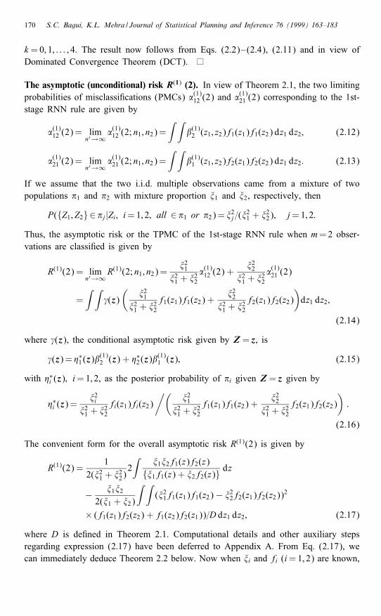
The asymptotic (unconditional) risk R(1) (2). In view of Theorem 2.1, the two limitingprobabilities of misclassi�cations (PMCs) �(1)12 (2) and �

(1)21 (2) corresponding to the 1st-

stage RNN rule are given by

�(1)12 (2)= limn′→∞

�(1)12 (2; n1; n2)=∫ ∫

�(1)2 (z1; z2)f1(z1)f1(z2) dz1 dz2; (2.12)

�(1)21 (2)= limn′→∞

�(1)21 (2; n1; n2)=∫ ∫

�(1)1 (z1; z2)f2(z1)f2(z2) dz1 dz2: (2.13)

If we assume that the two i.i.d. multiple observations came from a mixture of twopopulations �1 and �2 with mixture proportion �1 and �2, respectively, then

P({Z1; Z2}∈ �j|Zi; i=1; 2; all ∈ �1 or �2)= �2j =(�21 + �22); j=1; 2:

Thus, the asymptotic risk or the TPMC of the 1st-stage RNN rule when m=2 obser-vations are classi�ed is given by

R(1)(2) = limn′→∞

R(1)(2; n1; n2)=�21

�21 + �22�(1)12 (2) +

�22�21 + �

22�(1)21 (2)

=∫ ∫

(z)(

�21�21 + �

22f1(z1)f1(z2) +

�22�21 + �

22f2(z1)f2(z2)

)dz1 dz2;

(2.14)

where (z), the conditional asymptotic risk given by Z = z, is

(z)= �∗1 (z)�(1)2 (z) + �

∗2 (z)�

(1)1 (z); (2.15)

with �∗i (z); i=1; 2, as the posterior probability of �i given Z = z given by

�∗i (z)=�2i

�21 + �22fi(z1)fi(z2)

/(�21

�21 + �22f1(z1)f1(z2) +

�22�21 + �

22f2(z1)f2(z2)

):

(2.16)

The convenient form for the overall asymptotic risk R(1)(2) is given by

R(1)(2) =1

2(�21 + �22)2∫

�1�2f1(z)f2(z){�1f1(z) + �2f2(z)} dz

− �1�22(�1 + �2)

∫ ∫(�21f1(z1)f1(z2)− �22f2(z1)f2(z2))2

× (f1(z1)f2(z2) + f1(z2)f2(z1))=D dz1 dz2; (2.17)

where D is de�ned in Theorem 2.1. Computational details and other auxiliary stepsregarding expression (2:17) have been deferred to Appendix A. From Eq. (2.17), wecan immediately deduce Theorem 2.2 below. Now when �i and fi (i=1; 2) are known,

S.C. Bagui, K.L. Mehra / Journal of Statistical Planning and Inference 76 (1999) 163–183 171

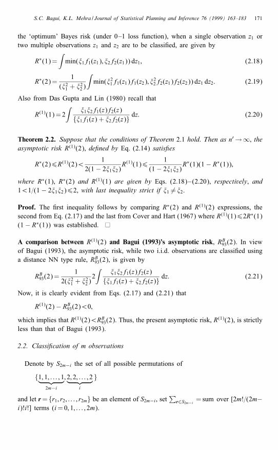
the ‘optimum’ Bayes risk (under 0–1 loss function), when a single observation z1 ortwo multiple observations z1 and z2 are to be classi�ed, are given by

R∗(1)=∫min(�1f1(z1); �2f2(z1)) dz1; (2.18)

R∗(2)=1

(�21 + �22)

∫min(�21f1(z1)f1(z2); �

22f2(z1)f2(z2)) dz1 dz2: (2.19)

Also from Das Gupta and Lin (1980) recall that

R(1)(1)= 2∫

�1�2f1(z)f2(z){�1f1(z) + �2f2(z)} dz: (2.20)

Theorem 2.2. Suppose that the conditions of Theorem 2.1 hold. Then as n′ →∞; theasymptotic risk R(1)(2), de�ned by Eq. (2.14) satis�es

R∗(2)6R(1)(2)¡1

2(1− 2�1�2)R(1)(1)6

1(1− 2�1�2)R

∗(1)(1− R∗(1));

where R∗(1), R∗(2) and R(1)(1) are given by Eqs. (2.18)–(2.20), respectively, and1¡1=(1− 2�1�2)62, with last inequality strict if �1 6= �2.

Proof. The �rst inequality follows by comparing R∗(2) and R(1)(2) expressions, thesecond from Eq. (2.17) and the last from Cover and Hart (1967) where R(1)(1)62R∗(1)(1− R∗(1)) was established.

A comparison between R(1)(2) and Bagui (1993)’s asymptotic risk, RB93(2). In viewof Bagui (1993), the asymptotic risk, while two i.i.d. observations are classi�ed usinga distance NN type rule, RB93(2), is given by

RB93(2)=1

2(�21 + �22)2∫

�1�2f1(z)f2(z){�1f1(z) + �2f2(z)} dz: (2.21)

Now, it is clearly evident from Eqs. (2.17) and (2.21) that

R(1)(2)− RB93(2)¡0;which implies that R(1)(2)¡RB93(2). Thus, the present asymptotic risk, R

(1)(2), is strictlyless than that of Bagui (1993).

2.2. Classi�cation of m observations

Denote by S2m−i the set of all possible permutations of

{1; 1; : : : ; 1︸ ︷︷ ︸2m−i

; 2; 2; : : : ; 2︸ ︷︷ ︸i

}

and let r= {r1; r2; : : : ; r2m} be an element of S2m−i, set∑

r∈S2m−i=sum over [2m!=(2m−

i)!i!] terms (i=0; 1; : : : ; 2m).

172 S.C. Bagui, K.L. Mehra / Journal of Statistical Planning and Inference 76 (1999) 163–183

The conditional probability, given Z = z, of deciding that Z = {Z1; Z2; : : : ; Zm} comesfrom �1 using 1st stage RNN rule de�ned by Eq. (1.1) is given by

�(1)1 (z1; z2; : : : ; zm; n1; n2) = E(�(1)|Z1 = z1; Z2 = z2; : : : ; Zm= zm)

= E(�(1)I(A(1)1 A(1)2 ::: A

(1)m )

|Z1 = z1; : : : ; Zm= zm)+E(�(1)I(A(1)1 A

(1)2 ::: A

(1)m )c

|Z1 = z1; : : : ; Zm= zm): (2.22)

Using Lemma 2.1 and following the same reasoning for Theorem 2.1, we obtain

Theorem 2.3. (i) Suppose that the conditions of Theorem 2.1 holds and z1; z2; : : : ; zmare continuity points of both f1 and f2. Then the asymptotic conditional probability,given Z = z, of classifying {Z1; Z2; : : : ; Zm} to �1 using the 1st-stage RNN rule isgiven by

�(1)1 (z1; z2; : : : ; zm) = limn→∞ �

(1)1 (z1; z2; : : : ; zm; n1; n2)

=m−1∑i=0

�2m−i +12 �m;

where for i=0; 1; : : : ; m,

�2m−i= �2m−i1 �i2

∑r∈S2m−i

fr1 (z1)fr2 (z1)fr3 (z2)fr4 (z2)=D′

with D′= {∏mi=1(�1f1(zi) + �2f2(zi))}2; Note that

∑2mk=0 �2m−k =1 and the limiting

conditional probability given Z = z of deciding that Z comes from �2 is given by�(1)2 (z1; z2; : : : ; zm)= 1− �(1)1 (z1; z2; : : : ; zm)=

∑2mi=m+1 �2m−i +

12 �m.

(ii) The limiting PMCs of the 1st-stage RNN rule for m-observations are givenbelow

�(1)12 (m)= limn′→∞

�(1)12 (m; n1; n2)=∫ ∫

�(1)2 (z1; : : : ; zm)m∏i=1f1(zi) dz1 : : : dzm;

�(1)21 (m)= limn′→∞

�(1)21 (m; n1; n2)=∫ ∫

�(1)1 (z1; : : : ; zm)m∏i=1f2(zi) dz1 : : : dzm:

If we assume that m i.i.d. multiple observations came from a mixture of two populations�1 and �2 with mixture proportion �1 and �2, respectively, then

P({Z1; : : : ; Zm}∈ �j|Zi; i=1; : : : ; m; all∈ �1 or �2)= �mj =(�m1 + �m2 ); j=1; 2:

Thus, the asymptotic risk or the TPMC of the 1st stage RNN rule when m observationsare classi�ed is given by

R(1)(m)= limn′→∞

R(1)(m; n1; n2)=�m1

�m1 + �m2�(1)12 (m) +

�m2�m1 + �

m2�(1)21 (m): (2.23)

One would expect that the inequality R(1)(m)¡R(1)(m−1) should hold in general and,indeed, this is supported by the Monte Carlo simulation results of in Section 5.

S.C. Bagui, K.L. Mehra / Journal of Statistical Planning and Inference 76 (1999) 163–183 173

3. Asymptotic TPMC of the M-stage RNN rule

Let �(M)1 (z1; : : : ; zm; n1; n2) be the conditional probability given Z1 = z1; : : : ; Zm= zmthat MRNN rule classi�es z=(z1; : : : ; zm) into �1. Recalling the de�nition of �(M) inEq. (2.1) it is easy to see that

�(M)1 (z1; : : : ; zm; n1; n2) = P(�(1) = 1|Z = z) +M∑i=2P(�(1) = 1

2 ; : : : ; �(i) = 1|Z = z)

+ 12P(�

(1) = 12 ; : : : ; �

(M) = 12 |Z = z); (3.1)

where, for l=1 or 12

P(�(1) = 12 ; : : : ; �

(i−1) = 12 ; �

(i) = l|Z = z)

=P(�(1) = 12 |Z = z)

i−1∏j=2P(�( j) = 1

2 |�( j−1) = 12 ; : : : ; �

(1) = 12 ;Z = z)

×P(�(i) = l|�(i−1) = 12 ; : : : ; �

(1) = 12 ;Z = z): (3.2)

Now, we state a lemma whose proof follows from those of Lemmas 3.1 and 3.2 ofDas Gupta and Lin (1980). Let �( j) = 1

2 (j=1; 2; : : : ; i − 1). Delete the observationscorresponding to U (i)

l and V (i)l (l=1; : : : ; m; j=1; : : : ; i− 1) and denote the remainingn1−(i−1)m X -observations and n2−(i−1)m Y -observations by X (i)r (r=1; 2; : : : ; n1−(i − 1)m) and Y (i)r (r=1; 2; : : : ; n2 − (i − 1)m), respectively.

Lemma 3.1. Given Zl= zl; �( j) = 12 ; U

(i)l = u(i)l ; V

(i)l = v(i)l (l=1; : : : ; m; j=1; : : : ; i−1),

the following statements hold:(i) X (i)r and Y (i)r are conditionally mutually independent,(ii) the conditional density of X (i)r and Y (i)r are f(i)1 and f(i)2 , respectively, where

for s=1; 2

f(i)s (x) =f(i)s

/[1−

m∑l=1p(i−1)s (l)

]

de�ned on [(u(i−1)1 ; v(i−1)1 )∪ · · · ∪ (u(i−1)m ; v(i−1)m )] (3.3)

where p(i−1)s (l)=F (i−1)s (v(i−1)l )−F (i−1)s (u(i−1)l ); (l=1; : : : ; m) and F (i−1)s is the c.d.f.corresponding to f(i−1)s , de�ned inductively by Eq. (3.3).

We are now going to deal explicitly with case m=2 only. Note that

P(�(i) = 1|�(i−1) = 12 ; : : : ; �

(1) = 12 ; Z1 = z1; Z2 = z2)

=EP(�(i) = 1|U (i)l ; V

(i)l ; �(i−1) = 1

2 ; : : : ; �(1) = 1

2 ; z1; z2) (3.4)

with

P(�(i) = 1|U (i)l ; V

(i)l ; �(i−1) = 1

2 ; : : : ; �(1) = 1

2 ; z1; z2)= (C(i)4 + C (i)3 )=B

(i); (3.5)

174 S.C. Bagui, K.L. Mehra / Journal of Statistical Planning and Inference 76 (1999) 163–183

where C (i)3 ; C(i)4 and B(i) can be obtained from C3; C4 and B (given in Eqs. (2.6) and

(2.7), respectively) by replacing n1; n2; u1; v1; u2; v2; f1; f2 by n1−2(i−1), n2−2(i−1),u(i)1 ; v

(i)1 ; u

(i)2 ; v

(i)2 ; f

(i)1 ; f

(i)2 , respectively (using (i) of Lemma 3.1). From (ii) of

Lemma 3.1, one could write f(i)s (x)=fs(x)=∏i−1r=1{1−

∑2l=1p

(r)s (l)} and when n′ →∞

U (i)l ; V

(i)l

a:s:→ zl (l=1; 2) and∑2l=1 p

(r)s (l)→ 0 and therefore f(i)s (U

(i)l ); f

(i)s (V

(i)l )→fs(zl)

a.s. Thus, the limiting value of (C (i)4 + C (i)3 )=B(i) would be (C4 + C3)=B. From Eqs.

(3.4), (3.5) and DCT, we obtain

limn′→∞

P(�(i) = 1|�(i−1) = 12 ; : : : ; �

(1) = 12 ; z1; z2)= (C4 + C3)=B= �4 + �3; (3.6)

and by similar arguments

limn′→∞

P(�(i) = 12 |�(i−1) = 1

2 ; : : : ; �(1) = 1

2 ; z1; z2)= �2; (3.7)

where �4; �3 and �2 are given by Eq. (2.10). Thus we can deduce the following:

Theorem 3.1. Suppose z1 and z2 are points of continuity of both f1 and f2, then thelimiting conditional probability given Zi= zi (i=1; 2) for classifying {Z1; Z2} into �1using the MRNN rule is given by

�(M)1 (z1; z2) = limn′→∞

�(M)1 (z1; z2; n1; n2)

= (�4 + �3)M−1∑i=1

�i2 +12 �M2 : (3.8)

Proof. Introducing the sets A(1)1 ; A(1)2 and arguing as in Eqs. (2.2)–(2.4), (3:8) follows

from Eqs. (3.1)–(3.2) and (3:6)–(3:7).

Thus the limiting risk, R(M)(2), as n′ →∞, for the MRNN rule is given by

R(M)(2)= limn′→∞

R(M)(2; n1; n2)=�21

�21 + �22�(M)12 (2) +

�22�21 + �

22�(M)21 (2); (3.9)

where

�(M)12 (2)= limn′→∞

�(M)12 (2; n1; n2)=∫ ∫

[1− �(M)1 (z1; z2)]f1(z1)f1(z2) dz1 dz2;

�(M)21 (2)= limn′→∞

�(M)21 (2; n1; n2)=∫ ∫

�(M)1 (z1; z2)f2(z1)f2(z2) dz1 dz2:

Now using Eqs. (3.8) and (3.9), we at once have

R(M)(2)− R(M−1)(2)

=−(�21 + �22)−1∫ ∫

�(M−1)2 (�4 + �3 +

12 �2 − 1

2 )

×{�21f1(z1)f1(z2)− �22f2(z1)f2(z2)} dz1 dz2

S.C. Bagui, K.L. Mehra / Journal of Statistical Planning and Inference 76 (1999) 163–183 175

=− 12 (�

21 + �

22)

−1∫ ∫

�(M−1)2 {�21f1(z1)f1(z2)− �22f2(z1)f2(z2)}2

×{�21f1(z1)f1(z2) + �22f2(z1)f2(z2) + 2�1�2[f1(z1)f2(z2)+f1(z2)f2(z1)]}=D dz1 dz2; (3.10)

the last equality following by substituting in the preceding integrand for �4; �3 and �2given by Eq. (2.10). We can now deduce the following Theorem 3.2 fromEqs. (3.8)–(3.10):

Theorem 3.2. The asymptotic TPMC R(M)(2) of the MRNN rule satis�es(i) R(M)(2)¡R(M−1)(2),(ii) R∗(2)6R(∞)(2)= limM→∞ R

(M)(2),where R∗(2) is the Bayes risk given by Eq. (2.19).

Proof. Eq. (3.10) clearly implies R(M)(2)¡R(M−1)(2). This proves part (i). To provepart (ii) note that, from Eqs. (3.8) and (3.9) we obtain by using DCT,

R(∞)(2) = limM→∞

R(M)(2)

= (�21 + �22)

−1∫ ∫

{(�1 + �0)�21f1(z1)f1(z2) + (�4 + �3)�22f2(z1)f2(z2)}

×(1− �2)−1 dz1 dz2¿ (�21 + �

22)

−1∫ ∫

min{�21f1(z1)f1(z2); �22f2(z1)f2(z2)} dz1 dz2= R∗(2):

4. Estimation of PMCs of the �rst-stage RNN rule

In this section, we consider the estimation of the overall asymptotic risk (i.e. TPMC)of the 1st-stage rule for general m (see Eq. (1.1) above), with risk R(1)(m) given byEq. (2.23) as its asymptotic version, and propose an asymptotically unbiased consistentestimator for R(1)(m). To accomplish this, set

px =1(n1

m

) ∑16i1¡···¡im6n1

(i1 ; i2 ;:::; im)x and py =

1(n2

m

) ∑16i1¡···¡im6n2

(i1 ; i2 ;:::; im)y ;

(4.1)

where (i1 ; i2 ;:::; im)x =1− �(1)(Xi1 ; Xi2 ; : : : ; Xim ;X�’s, Y�’s, � 6= i1; i2; : : : ; im) and (i1 ; i2 ;:::; im)

y

de�ned analogously, with �(1) as de�ned by Eq. (2.1). Then the proposed estimator is

pxy={(

n1m

)px +

(n2m

)py

}/{(n1m

)+(n2m

)}: (4.2)

176 S.C. Bagui, K.L. Mehra / Journal of Statistical Planning and Inference 76 (1999) 163–183

Estimator (4:2) is commonly referred to in literature as the cross-validation estimator.Note that

E(px)=∫[1− �(1)1 (z1; z2; : : : ; zm; n1 − m; n2)] dz1 : : : dzm

and

limn′→∞

E(px)=∫[1− �(1)1 (z1; z2; : : : ; zm)] dz1 : : : dzm= �(1)12 (m):

Similarly, we can show that limn′→∞ E(py)= �(1)21 (m). Thus,

limn′→∞

E(pxy)=�m1

�m1 + �m2�(1)12 (m) +

�m2�m1 + �

m2�(1)21 (m)=R

(1)(m):

Therefore, estimator (4:2) is asymptotically unbiased for R(1)(m).To establish the L2-consistency of this estimator, we need to establish simply that

E(pxy − pxy)2 = o(1), as n′ →∞, where pxy is de�ned as pxy, with px(py) replacedthere in by px =p

(n)x =E[px|Xi1 ; Xi2 ; : : : ; Xim ] (py =p(n)y de�ned analogously). This fol-

lows since for given n1 and n2; p(n)x and p(n)y are U-statistics, so that the L2-convergence

of pxy=p(n)xy to R(1)(m) follows from Theorem 2.3, Eq. (2.23) and the well-known

Hoe�ding’s theory of U-statistics (see Ser ing, 1980, p. 190). In fact, for the L2-consistency of pxy, clearly it su�ces to establish simply that

E(px − p(n)x )2 = o(1); as n′ →∞: (4.3)

For convenience we shall treat explicitly only the m=2, the extension of argumentsto proofs for general m being analogous and conceptually straight forward. The Proofregarding Eq. (4.3) with m=2 has been presented in the Appendix B. Now we stateour result in the form of a theorem below.

Theorem 4.1. Suppose the densities f1 and f2 are almost everywhere continuous, thenthe estimator pxy, given by Eq. (4.2), of the asymptotic R

(1)(m) is L2-consistent, asn′ →∞.

Similarly estimates of the PMCs of the multistage RNN rule can be obtained and itcan be shown that they are asymptotically unbiased and consistent.

5. Monte Carlo simulation results

The asymptotic properties of the proposed MRNN classi�cation rules derived abovethrow some light on their operating characteristics for large samples. These resultswould be of limited value in applications if they were not aided by favorable resultsin speci�c situations for small and moderate sample sizes. Accordingly, in the presentsection we examine, through Monte Carlo simulation, the small performance of the

S.C. Bagui, K.L. Mehra / Journal of Statistical Planning and Inference 76 (1999) 163–183 177

Table 1APMs with 1st-stage RNN rule for discrimination between two populations

m A B C D E Fr (1)(m) r (1)(m) r (1)(m) r (1)(m) r (1)(m) r (1)(m)

1 0.3075 0.3750 0.4800 0.2950 0.4800 0.20252 0.2750 0.3375 0.4075 0.2050 0.4425 0.16753 0.1925 0.2875 0.3825 0.1575 0.4375 0.08504 0.1825 0.2675 0.3500 0.1050 0.4100 0.05755 0.1550 0.2075 0.3425 0.0900 0.3975 0.0500

A=LA(0; 1) vs. LA(1; 1); B=LG(0; 1) vs. LG(2; 1); C =N(0; 1) vs. LG(2; 1); D=EX(0; 1) vs. GA(2; 1);E=EX(0; 1) vs. WE(2; 1); F =WE(2; 1) vs. GA(3; 1); G=N(0; 1) vs. N(1; 1); H =N(0; 1) vs. N(2; 1);J =N(0; 1) vs. LA(2; 1).

Table 2Comparison between MRNN rule and Choi’s parametric rule

m G H J

I II I II I II

2 0.3325 0.2520 0.1555 0.1303 0.2150 0.22473 0.3025 0.1950 0.1225 0.1256 0.1725 0.20084 0.2175 0.1620 0.0850 0.0841 0.1550 0.19305 0.2175 0.1311 0.0375 0.0677 0.1375 0.2167

I=APMs for the MRNN rule. II =APM’s using Choi’s rule. N(�; �2)=Normal with mean � and vari-ance �2; LA(a; b)=Laplace with location a and scale b; LG(a; b)=Logistic with location a and scaleb; EX(a; b)=Exponential with location a and scale b; GA(a; b)=Gamma with shape a and scale b;WE(a; b)=Weibull with shape a and scale b.

proposed 1st-stage RNN rule by applying it to a number of pairs of some standarddistributions. For given Xi’s and Yj’s (random sample of size 50 each) from �1 and�2. The average proportion of misclassi�cation (APM) (denoted r (1)(m)) is calculatedfor m=1; 2; : : : ; 5. The results are given in Tables 1 and 2

6. Concluding remarks

The results of Theorems 2.2 and 3.2 indicate (i) that, not only for the 1st-stageRNN rule but also possibly in general, the additional information provided by multipleobservations does help to reduce the large sample overall probability of misclassi�-cation (TPMC) and (ii) that the higher the number M of stages employed in themulti-stage RNN rule, the lower the corresponding large sample TPMC. The MonteCarlo results above in Table 1 indicate that the �rst of these desirable properties –which one would expect of any satisfactory multiple observation classi�cation proce-dure – holds for small and moderate training sample sizes as well. Table 2 comparesthe proposed multiple observation RNN classi�cation rule with the corresponding Choi(1972) parametric rule. The results suggest that, under normality when the distributionsof �1 and �2 are close, Choi’s rule performs better, but when they are further apart or

178 S.C. Bagui, K.L. Mehra / Journal of Statistical Planning and Inference 76 (1999) 163–183

when the normality assumption may not hold, the RNN rule perform equally well orbetter.The MRNN rule depends only on ranks. Thus, this procedure is particularly useful

when observations are available in terms of ranks. It is also invariant under the mono-tonic transformations. The computational complexities of the MRNN rule are far lessthen that of the distance-based NN-type rule proposed by Bagui (1993) and Bagui etal. (1995). In fact, in Section 2 we showed that the asymptotic risk of the 1st-stageRNN rule is strictly less than that of Bagui (1993), and also demonstrated its superiorupper bound. If a tie occurs at the time of classi�cation, apply the multi-stage rule.This will reduce the chance of randomization as we have demonstrated this propertyin Section 3. Moreover, MRNN rule is quite simple to employ and, as seen above,performs remarkably well.

Acknowledgements

The authors wish to thank an associate editor for invaluable suggestions on the earlierversion of the paper.

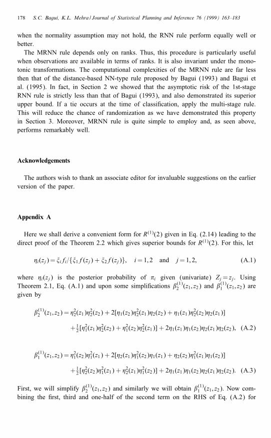
Appendix A

Here we shall derive a convenient form for R(1)(2) given in Eq. (2.14) leading to thedirect proof of the Theorem 2.2 which gives superior bounds for R(1)(2). For this, let

�i(zj)= �ifi={�1f(zj) + �2f(zj)}; i=1; 2 and j=1; 2; (A.1)

where �i(zj) is the posterior probability of �i given (univariate) Zj = zj. UsingTheorem 2.1, Eq. (A.1) and upon some simpli�cations �(1)2 (z1; z2) and �

(1)1 (z1; z2) are

given by

�(1)2 (z1; z2) = �22(z1)�

22(z2) + 2[�1(z2)�

22(z1)�2(z2) + �1(z1)�

22(z2)�2(z1)]

+12 [�

21(z1)�

22(z2) + �

21(z2)�

22(z1)] + 2�1(z1)�1(z2)�2(z1)�2(z2); (A.2)

�(1)1 (z1; z2) = �21(z2)�

21(z1) + 2[�2(z1)�

21(z2)�1(z1) + �2(z2)�

21(z1)�1(z2)]

+12 [�

22(z2)�

21(z1) + �

22(z1)�

21(z2)] + 2�1(z1)�1(z2)�2(z1)�2(z2): (A.3)

First, we will simplify �(1)2 (z1; z2) and similarly we will obtain �(1)1 (z1; z2). Now com-

bining the �rst, third and one-half of the second term on the RHS of Eq. (A.2) for

S.C. Bagui, K.L. Mehra / Journal of Statistical Planning and Inference 76 (1999) 163–183 179

�(1)2 (z1; z2), we obtain, after some rearrangement and use of �1(z) + �2(z)= 1,

�22(z1)�22(z2) +

12 [�

21(z1)�

22(z2) + �

21(z2)�

22(z1)]

+ [�1(z2)�22(z1)�2(z2) + �1(z1)�22(z2)�2(z1)]

= 12�22(z2)[�

22(z1) + �

21(z1) + 2�1(z1)�2(z1)]

+ 12�22(z1)[�

22(z2) + �

21(z2) + 2�1(z2)�2(z2)]

= 12 [�

22(z1) + �

22(z2)]; (A.4)

further also note that in Eq. (A.2), the sum of the remaining terms (namely, the fourthterm plus one-half of the second term) equals

�1(z2)�22(z1)�2(z2) + �1(z1)�22(z2)�2(z1) + 2�1(z1)�1(z2)�2(z1)�2(z2)

= �1(z2)�2(z1)�2(z2)[�2(z1) + �1(z1)] + �1(z1)�2(z1)�2(z2)[�1(z2) + �2(z2)]

= �2(z1)�2(z2)[�1(z2) + �1(z1)]: (A.5)

Now combining Eqs. (A.4) and (A.5), one obtains

�(1)2 (z1; z2)= �2(z1)�2(z2)[�1(z1) + �1(z2)] +12 [�

22(z1) + �

22(z2)]: (A.6)

To achieve our objective, we shall further modify the expression in Eq. (A.6): Addingone-half of the �rst term to the second term on the RHS of Eq. (A.6) yields

12 [�2(z1){�2(z1) + �1(z1)�2(z2)}+ �2(z2){�2(z2) + �2(z1)�1(z2)}]= 1

2 [�2(z1) + �2(z2)][1− �1(z1)�1(z2)]; (A.7)

the last equality following on the account of Eqs. (A.8) and (A.9) below:

�2(z1) + �1(z1)�2(z2)= �2(z1) + �1(z1)− �1(z1)�1(z2)= 1− �1(z1)�1(z2) (A.8)

and

�2(z2) + �2(z1)�1(z2)= �2(z2) + �1(z2)− �1(z1)�1(z2)= 1− �1(z1)�1(z2): (A.9)

In view of Eqs. (A.6) and (A.7) we have

�(1)2 (z1; z2)=12 [�2(z1) + �2(z2)] +

12 t(z1; z2); (A.10)

where t(z1; z2)= {�2(z1)�2(z2)[�1(z1)+�1(z2)]−�1(z1)�1(z2)[�2(z1)+�2(z2)]}. Similarly,one obtains

�(1)1 (z1; z2)=12 [�1(z1) + �1(z2)]− 1

2 t(z1; z2): (A.11)

180 S.C. Bagui, K.L. Mehra / Journal of Statistical Planning and Inference 76 (1999) 163–183

Now using Eqs. (A.10) and (A.11) in Eq. (2.15) then substituting for �∗i (z) and (z)from Eqs. (2.16) and (2.15) in Eq. (2.14), we obtain after some simpli�cation,

R(1)(2) = 12 (�

21 + �

22)

−1{∫ ∫

�21f1(z1)f1(z2)[�2(z1) + �2(z2)] dz1 dz2

+∫ ∫

�22f2(z1)f2(z2)[�1(z1) + �1(z2)] dz1 dz2

}

+12(�

21 + �

22)

−1∫ ∫

{�21f1(z1)f1(z2)− �22f2(z1)f2(z2)}t(z1; z2) dz1 dz2;

= 12(�

21 + �

22)

−12∫

�1�2f1(z)f2(z){�1f1(z) + �2f2(z)} dz

− 12�1�2(�

21 + �

22)

−1∫ ∫

{�21f1(z1)f1(z2)− �22f2(z1)f2(z2)}2

× (f1(z1)f2(z2) + f1(z2)f2(z1))=D dz1 dz2;

where the last equality is obtained by the identity

t(z1; z2)=−{�21f1(z1)f1(z2)− �22f2(z1)f2(z2)}(f1(z1)f2(z2) + f1(z2)f2(z1))=D

and substituting for �i(zj); i=1; 2 and j=1; 2; from Eq. (A.1) in the preceding ex-pression. Thus, the proof of expression (2:17) is completed.

Appendix B

To establish Eq. (4.3) for m=2 (for general m the proof is analogous and straightforward), we note that upon setting

t (n)ij =�(1)n−2(Xi; Xj;X�’s; Y�’s; � 6= i; j) and E[t (n)ij ] =E[t

(n)ij |Xi; Xj]; (B.1)

we obtain

E(px − p(n)x )2 =(n12

)−2{ ∑16i¡j6n1

E[t (n)ij − E(t (n)ij )]2

+∑′

{i¡j; i′¡j′}E(t (n)ij − E(t (n)ij ))(t (n)i′j′ − E(t (n)i′j′))

+∑′′

{i¡j; i′¡j′}E(t (n)ij − E(t (n)ij ))(t (n)i′j′ − E(t (n)i′j′))

}

= �1 + �2 + �3 (say); (B.2)

where in the summation∑′ there are only three distinct running subscripts among

i¡j and i′¡j′, i.e., either i= i′ or j′ or j= i′ or j′ and in the summation∑′′ all

subscripts are distinct. Since each |t (n)ij |61, clearly |�1|=O(n−21 ) and |�2|=O(n−11 ), as

S.C. Bagui, K.L. Mehra / Journal of Statistical Planning and Inference 76 (1999) 163–183 181

n′ →∞. Since the ( n12) and ( n1−2

2) terms in

∑′′ are all identical, so that for proving

|�3|=o(1), as n′ →∞, it su�ces to show thatE(t (n)12 − E(t (n)12 ))(t (n)34 − E(t (n)34 ))=E[t (n)12 t

(n)34 ]− E[t (n)12 E(t (n)34 )]− E[E(t (n)12 )t (n)34 ] + E[E(t (n)12 )E(t (n)34 )]

= �(n)31 − �(n)32 − �(n)33 + �(n)34 (say)= o(1); as n′ →∞: (B.3)

To demonstrate the last assertion in Eq. (B.3) which will then establish Eq. (4.3), weshall show below that, apart from the signs, each term on the RHS in Eq. (B.3)converges to the same constant, as n′ →∞. To see this, let E(:) (see Eq. (B.1)above) denote the conditional expectation given the ‘pivotal’ {X1; X2} or {X1; X4}(‘pivotal’= playing the role of {Z1; Z2} of Section 2) and �E(:) denote the conditionalexpectation given the non-pivotal {X1; X2} or {X3; X4}. We shall �rst deal with thesecond term, the proof for the third term being analogous and that of the fourth clearlyfollowing from Theorem 2.1: First, note that

�(n)32 =E[ �E{t (n)12 E(t (n)34 )}] =E[ �E(t (n)12 )E(t (n)34 )]; (B.4)

where, using Lemma 2.1 and the notation and arguments of Section 2 leading toTheorem 2.1, as n′ →∞,

�E(t(n)12 ) = E{�(1)n1−2; n2I[A(1)1 ∩ A(1)2 ]I[X3 ; X4 =∈{(u(1)1 ; v(1)1 )∪(u(1)2 ; v(1)2 )}]

|X1; X2; X3; X4}+E{�(1)n1−2; n2 (I[A(1)1 ∩A(1)2 ]c

+ I[X3 ; X4∈{(u(1)1 ; v(1)1 )∪ (u(1)2 ; v(1)2 )}])|X1; X2; X3; X4}

= [ �B(n1 − 2; n2)]−2{ �C4(n1 − 2; n2) + �C3(n1 − 2; n2)+ 1

2�C2(n1 − 2; n2)}+ o(1); (B.5)

where �B(n1 − 2; n2)=∑4

k=0�Ck(n1 − 2; n2) and �C4(n1 − 2; n2); 06k64, as de�ned

in Eq. (2.6) with Z1 and Z2 replaced by X1 and X2, respectively, and X1; X2; X3; X4given. Under the conditions of Theorem 2.1, thus, with {Z1; Z2} replaced by {X1; X2}or {X3; X4}, we obtain from Eqs. (B.4) and (B.5) that, as n′ →∞, for j=2; 3; 4,

limn′→∞

�(n)3j =E[�(1)1 (X1; X2)]E(�

(1)1 (X3; X4)]: (B.6)

We now establish that �(n)31 also converges to the same limit on the RHS of Eq. (4:9),for which extending the arguments and notations of Theorem 2.1 for evaluating theanalogous conditional expectation expressions given X1; X2; X3; X4 (instead of Z1 andZ2), we obtain �rstly

�E[t (n)12 t(n)34 ] = [B

∗(n1 − 4; n2)]−1{[ �C44(n1 − 4; n2) + �C43(n1 − 4; n2)+ �C34((n1 − 4; n2) + �C33(n1 − 4; n2)]+12 [ �C42(n1 − 4; n2) + �C32(n1 − 4; n2)

+ �C23(n1 − 4; n2) + �C24(n1 − 4; n2)] + 14�C22(n1 − 4; n2)}; (B.7)

182 S.C. Bagui, K.L. Mehra / Journal of Statistical Planning and Inference 76 (1999) 163–183

where B∗(n1 − 4; n2)=∑

06k; k′64�Ckk′(n1 − 4; n2) and setting p

(i)j =Fi(vj) − Fi(uj);

i=1; 2 and j=1; 2; 3; 4;

�Ckk′(n1 − 4; n2) =3+k+k′∏k=4

(n− j)(1−

4∑j=1p(1)j

)n1−4−k−k′

×8−k−k′∏j′=0

(n2 − j′)(1−

4∑j=1p(2)j

)n2−(8−k−k′)

× ∑′{r1 ;:::; r8}

fr1 (u1)fr2 (v1)fr3 (u2)fr4 (v2)fr5 (u3)

×fr6 (v3)fr7 (u4)fr8 (v4); (B.8)

where∑′ denotes the sum over all distinct permutations {r1; r2; : : : ; r8} of (k+ k ′) 1’s

and (8− k − k ′) 2’s. By following reasoning similar to that of Theorem 2.1, it followsfrom Eqs. (B.7) and (B.8) that

�(n)31 =E[t(n)12 t

(n)34 ] =E[ �E(t

(n)12 t

(n)34 )] → the RHS of Eq: (B:6); (B.9)

as n′ →∞. In view of Eqs. (B.2), (B.3), (B.6) and (B.9), Eq. (4.3) standsestablished.

References

Anderson, T.W., 1966. Some nonparametric multivariate procedures based on statistical equivalent blocks.Krishnaih, P.R. (Ed.), Proc. 1st Int. Symp. Anal. Academic Press, New York.

Bagui, S.C., 1993. An NN classi�cation rule for multiple observations. Calcutta Statist. Assoc. Bull. 43(169–170) 45–55.

Bagui, S.C., Mehra, K.L., Rao, M.S., 1995. A nearest neighbor classi�cation rule for multiple observationsbased on a sub-sample approach. Sankhya A 57, part 2, 316–332.

Bagui, S.C., Mehra, K.L., Vaughn, B.K., 1997. An M-stage version of the k-RNN rule in statisticaldiscrimination. J. Statist. Plan. Infer. 65, 323–333.

Bagui, S.C., Vaughn, B.K., 1998. Statistical classi�cation based on k-Rank nearest neighbor rule. Statist. 16,181–189.

Choi, S.C., 1972. Classi�cation of multiply observed data. Biom. Z. 14, 8–11.Cover, T.M., Hart, P.E., 1967. Nearest neighbor pattern classi�cation. IEEE Trans. Inform. Theory IT-13,21–26.

Das Gupta, S., 1964. Nonparametric classi�cation rules. Sankhya A 26, 25–30.Das Gupta, S., Lin, H.E., 1980. Nearest neighbor rules for statistical classi�cation based on ranks. Sankhya A42, 219–230.

Devroye, L., 1981. On the asymptotic probability of error in nonparametric discrimination. Ann. Statist. 9,1320–1327.

Fix, E., Hodges, J.L., 1951. Nonparametric discrimination: consistency properties. U.S. Air Force School ofAviation Medicine, Report No. 4 Randolph Field, Texas. Report No. 11, 1952.

Fritz, J., 1975. Distribution-free exponential error bound for nearest neighbor pattern classi�cation. IEEETrans. Inform. Theory IT-21, 552–557.

Govindarajulu, Z., Gupta, A.K., 1977. Certain nonparametric classi�cation rules and their asymptotice�ciencies. Can. J. Statist. 5, 167–178.

Gupta, A.K., 1986. On a classi�cation rule for multiple measurements. Comput. Math. Appl. 12A, 301–308.Gupta, A.K., Logan, T.P., 1990. On a multiple observations model in discriminant analysis. J. Statist. Comput.Simul. 34, 119–132.

S.C. Bagui, K.L. Mehra / Journal of Statistical Planning and Inference 76 (1999) 163–183 183

Hoe�ding, W., 1963. Probability inequalities for the sums of bounded random variables. J. Amer. Statist.Assoc. 58, 13–30.

Hudimoto, H., 1964. On a distribution-free two-way classi�cation. Ann. Inst. Statist. Math. 9, 31–36.Lin, H.E., 1979. Classi�cation rules based on U -statistics. Sankhya B 41 (parts 1 and 2) 41–52.McLachlan, G.J., 1992. Discriminant Analysis and Statistical Pattern Recognition. Wiley, New York.Ser ing, R.J., 1980. Approximation Theorems of Mathematical Statistics. Wiley, New York.Silverman, B.W., Jones, M.C., 1989. E. Fix, Hodges (1951): an important contribution to nonparametricdiscriminant analysis and density estimation. Int. Statist. Rev. 57, 233–247.

Wagner, T.J., 1971. Convergence of the nearest neighbor rule. IEEE Trans. Inform. Theory IT-17, 566–571.Xiru, C., 1985. Exponential posterior error bound for the k-NN discrimination rule. Scentia Sinica A XXVII,673–682.