Active Nearest Neighbors in Changing Environments

Active Nearest Neighbors in Changing Environments

Christopher Berlind [email protected]

Georgia Institute of Technology, Atlanta, GA, USA

Ruth Urner [email protected]

Max Planck Institute for Intelligent Systems, Tubingen, Germany

AbstractWhile classic machine learning paradigms as-sume training and test data are generated fromthe same process, domain adaptation addressesthe more realistic setting in which the learner haslarge quantities of labeled data from some sourcetask but limited or no labeled data from the tar-get task it is attempting to learn. In this work,we give the first formal analysis showing that us-ing active learning for domain adaptation yields away to address the statistical challenges inherentin this setting. We propose a novel nonparamet-ric algorithm, ANDA, that combines an activenearest neighbor querying strategy with nearestneighbor prediction. We provide analyses of itsquerying behavior and of finite sample conver-gence rates of the resulting classifier under co-variate shift. Our experiments show that ANDAsuccessfully corrects for dataset bias in multi-class image categorization.

1. IntroductionMost machine learning paradigms operate under the as-sumption that the data generating process remains stable.Training and test data are assumed to be from the same task.However, this is often not an adequate model of reality. Forexample, image classifiers are often trained on previouslycollected data before deployment in the real world, wherethe instances encountered can be systematically different.An e-commerce company may want to predict the successof a product in one country when they only have preferencedata on that product from consumers in a different country.These and numerous other examples signify the importanceof developing learning algorithms that adapt to and performwell in changing environments. This is usually referred to

Proceedings of the 32nd International Conference on MachineLearning, Lille, France, 2015. JMLR: W&CP volume 37. Copy-right 2015 by the author(s).

as transfer learning or domain adaptation.

In a common model for domain adaptation, the learner re-ceives large amounts of labeled data from a source distri-bution and unlabeled data from the actual target distribu-tion (and possibly a small amount of labeled data from thetarget task as well). The goal of the learner is to outputa good model for the target task. Designing methods forthis scenario that are statistically consistent with respect tothe target task is important, yet challenging. This difficultyoccurs even in the so-called covariate shift setting, wherethe change in the environments is restricted to the marginalover the covariates, while the regression functions (the la-beling rules) of the involved distributions are identical.

In this work, we give the first formal analysis showing thatusing active learning for domain adaptation yields a wayto address these challenges. In our model, the learner canmake a small number of queries for labels of target exam-ples. Now the goal is to accurately learn a classifier for thetarget task while making as few label requests as possible.We design and analyze an algorithm showing that being ac-tive adaptive can yield a consistent learner that uses targetlabels only where needed.

We propose a simple nonparametric algorithm, ANDA,that combines an active nearest neighbor querying strategywith nearest neighbor prediction. ANDA receives a labeledsample from the source distribution and an unlabeled sam-ple from the target task. It first actively selects a subset ofthe target data to be labeled based on the amount of sourcedata among the k′ nearest neighbors of each target exam-ple. Then it outputs a k-nearest neighbor classifier on thecombined source and target labeled data.

We prove that ANDA enjoys strong performance guaran-tees. We first provide a finite sample bound on the expectedloss of the resulting classifier in the covariate shift setting.Remarkably, the bound does not depend on source-targetrelatedness; it only depends on the size of the given unla-beled target sample and properties of the target distribution.This is in stark contrast to most theoretical results for do-


main adaptation, where additive error terms describing thedifference between the source and target frequently appear.

On the other hand, the number of target label queriesANDA makes does depend on the closeness of the in-volved tasks. ANDA will automatically adjust the numberof queries it makes based on local differences between thesource and target. We quantify this by giving sample sizessufficient to guarantee that ANDA makes no queries at allin regions with large enough relative source support. Sim-ply put, ANDA is guaranteed to make enough queries to beconsistent but will not make unnecessary ones.

ANDA’s intelligent querying behavior and its advantagesare further demonstrated by our visualizations and exper-iments. We visually illustrate ANDA’s query strategyand show empirically that ANDA successfully corrects fordataset bias in a challenging image classification task.

1.1. Summary of Main Contributions

The active nearest neighbor algorithm. ANDA operateson a labeled sample from the source distribution and an un-labeled sample from the target task and is parametrized bytwo integers k and k′. The query rule is to ensure that everytarget example has at least k labeled examples among its k′

nearest neighbors. We describe this formally by definingthe concept of a (k, k′)-NN-cover, which may be of inde-pendent interest for nearest neighbor methods.

Bounding the loss. Theorem 1 provides a finite samplebound on the expected 0-1 loss of the classifier output byANDA. This bound depends on the size of the unlabeledtarget sample, the Lipschitz constant of the regression func-tion, and the covering number of the support of the targetdistribution. It does not depend on the size or the generat-ing process of the labeled source sample. In particular, itdoes not depend on any relatedness measure between thesource and target data generating distributions. We alsoshow that, even dropping the Lipschitz condition, ANDAis still consistent (Corollary 1).

Bounding the number of queries. In Theorem 2 weshow that, with high probability, ANDA will not make anyqueries on points that are sufficiently represented by thesource data. This implies in particular that, if the sourceand target happen to be very similar, ANDA will not makeany queries at all. We also prove a “query consistency” re-sult. Together with the error consistency, this implies weget the desired behavior of our active adaptive scheme: itsloss converges to the Bayes optimal while queries are madeonly in regions where the source is uninformative.

Finding a small (k, k′)-NN-cover. In general, there aremany possible (k, k′)-NN-covers to which our theory ap-plies, so finding a small cover will use fewer labels for thesame error guarantee. We show that finding a minimum-

size cover is a special case of the MINIMUM MULTISETMULTICOVER problem (Rajagopalan & Vazirani, 1993).We employ a greedy strategy to find a small cover and ar-gue that it enjoys anO(logm)-approximation guarantee ona combined source/target sample of m points.

Image classification experiments. We demonstrateANDA’s effectiveness in practice by applying it to theproblem of dataset bias in image classification. On a col-lection of 40-class, 1000-dimension datasets (Tommasi &Tuytelaars, 2014), ANDA consistently outperforms base-line nearest neighbor methods, despite the data’s high di-mensionality and lack of strict adherence to covariate shift.This also shows that ANDA performs well even when ourtheory’s assumptions are not exactly satisfied.

The idea of incorporating active learning (selective query-ing strategies) into the design of algorithms for domainadaptation has recently received some attention (Chat-topadhyay et al., 2013a;b; Saha et al., 2011). However,to the best of our knowledge, there has not been any for-mal analysis of using active learning to adapt to distribu-tion changes. We believe active learning is a powerful andpromising tool for obtaining domain adaptive learners andthat this area deserves a sound theoretical foundation. Weview our work as a first step in this direction.

1.2. Related Work

There is a rich body of applied studies for transfer or do-main adaptation learning (Pan & Yang, 2010), and on se-lective sampling or active learning (Settles, 2010). We herefocus on studies that provide performance guarantees.

For domain adaptation, even under covariate shift, perfor-mance guarantees usually involve an extra additive termthat measures the difference between source and targettasks (Ben-David et al., 2006; Mansour et al., 2009), orthey rely on strong assumptions, such as the target sup-port being a subset of the source support and the densityratio between source and target being bounded from below(Sugiyama et al., 2008; Ben-David & Urner, 2014; Shi &Sha, 2012). Generally, the case where the target is partlysupported in regions that are not covered by the source isconsidered to be particularly challenging yet more realistic(Cortes et al., 2010). We show that our method guaranteessmall loss independent of source-target relatedness.

The theory of active learning has also received a lot of at-tention in recent years (Dasgupta, 2004; Balcan et al., 2007;2009; Hanneke, 2011). See (Dasgupta, 2011) for a surveyon the main directions. However, the main goal of incor-porating active queries in all these works is to learn a clas-sifier with low error while using fewer labels. In contrast,we focus on a different benefit of active queries and for-mally establish that being active is also useful to adapt to


changing environments.

Nearest neighbor methods have been studied for decades(Cover & Hart, 1967; Stone, 1977; Kulkarni & Posner,1995). While the locality of the prediction rule makes themhighly flexible predictors, nearest neighbor methods sufferfrom a lack scalability to high dimensional data. However,there has recently been renewed interest in these methodsand ways to overcome the curse of dimensionality both sta-tistically (Kpotufe, 2011; Chaudhuri & Dasgupta, 2014)and computationally (Dasgupta & Sinha, 2013; Ram et al.,2012; Ram & Gray, 2013). Selective sampling for near-est neighbor classification has been shown to be consis-tent under certain conditions on the querying rule (Das-gupta, 2012); however, this work considers a data streamthat comes from a fixed distribution. A 1-nearest neighboralgorithm has been analyzed under covariate shift (Ben-David & Urner, 2014); however, in contrast to our work,that study assumes a lower bound on a weight ratio betweensource and target. In our work, we argue that the flexibilityof nearest neighbor methods can be exploited for adapt-ing to changing environments; particularly so for choosingwhere to query for labels by detecting areas of the targettask that are not well covered by the source.

1.3. Notation

Let (X , ρ) be a separable metric space. We let Br(x) de-note the closed ball of radius r around x. We let Nε(X , ρ)denote the ε-covering-number of the metric space, that is,the minimum number of subsets C ⊆ X of diameter atmost ε that cover the space X . We consider binary classi-fication tasks, where PS and PT denote source and targetdistributions over X × {0, 1} and DS and DT denote theirrespective marginal distributions over X . Further, XS andXT denote the support ofDS andDT respectively. That is,for I ∈ {S, T}, we have XI := {x ∈ X : DI(Br(x)) > 0for all r > 0}. We use the notation S and T for i.i.d. sam-ples from PS and DT , respectively, and let |S| = mS ,|T | = mT , and m = mS + mT . We let S, T denote theempirical distributions according to S and T .

We work in the covariate shift setting, in which the regres-sion function η(x) = P[y = 1|x] is the same for bothsource and target distributions.

For any finite A ⊆ X and x ∈ X , the notationx1(x,A), . . . , x|A|(x,A) gives an ordering of the elementsof A such that ρ(x1(x,A), x) ≤ ρ(x2(x,A), x) ≤ · · · ≤ρ(x|A|(x,A), x). If A is a labeled sequence of domainpoints, A = ((x1, y1), (x2, y2), . . . , (xm, ym)), then weuse the same notation for the labels (that is yi(x,A) denotesthe label of the i-th nearest point to x in A). We use the no-tation k(x,A) = {x1(x,A), . . . , xk(x,A)} to denote theset of the k nearest neighbors of x in A.

Algorithm 1 ANDA: Active NN Domain Adaptationinput Labeled set S, unlabeled set T , parameters k, k′

Find T l ⊆ T s.t. S ∪ T l is a (k, k′)-NN-cover of TQuery the labels of points in T l

return hkS∪T l , the k-NN classifier on S ∪ T l

We are interested in bounding the target loss of a k-nearest neighbor classifier. For a labeled sequence A =((x1, y1), (x2, y2), . . . , (xm, ym)) we let hkA denote the k-NN classifier on A: hkA(x) := 1

[1kΣki=1yi(x,A) ≥ 1

2

],

where 1[·] is the indicator function. We denote the Bayesclassifier by h∗(x) = 1[η(x) ≥ 1/2] and the target loss ofa classifier h : X → {0, 1} by LT (h) = P(x,y)∼PT

[y 6=h(x)]. For a subset A ⊆ X that is measurable both withrespect to DS and DT and satisfies DT (A) > 0, we de-fine the weight ratio of A as β(A) := DS(A)/DT (A). Fora collection of subsets B ⊆ 2X (for example all balls in(X , ρ)), we let dVC(B) denote its VC-dimension.

2. The AlgorithmIn brief, our algorithm receives a labeled sample S (fromthe source distribution), an unlabeled sample T (from thetarget distribution), and two parameters k and k′. It thenchooses a subset T l ⊂ T to be labeled, queries the labelsof points in T l, and outputs a k-NN predictor on S∪T l (seeAlgorithm 1). The subset T l is chosen so that the resultinglabeled set S ∪ T l is a (k, k′)-NN-cover for the target (un-labeled) sample T .

Definition ((k, k′)-NN-cover). Let T ⊆ X be a set of el-ements in a metric space (X , ρ) and let k, k′ ∈ N withk ≤ k′. A set R ⊆ X is a (k, k′)-NN-cover for T if, forevery x ∈ T , either x ∈ R or there are k elements fromR among the k′ nearest neighbors of x in T ∪ R, that is|k′(x, T ∪R) ∩R| ≥ k (or both).

Our loss bound in Section 3 (Theorem 1) holds wheneverT l ∪ S is some (k, k′)-NN-cover of T . Algorithm 2 pro-vides a simple strategy to find such a cover: add to T l allpoints whose k′ nearest neighbors among S ∪ T includefewer than k source examples. It is easy to see that thiswill always result in a (k, k′)-NN-cover of T . Further-more, this approach has a query safety property: the setT l produced by Algorithm 2 satisfies T l ∩ Q = ∅ whereQ = {x ∈ T : |k′(x, S ∪ T ) ∩ S| ≥ k} is the set of tar-get examples that have k source neighbors among their k′

nearest neighbors in S ∪ T . In other words, Algorithm 2will not query the label of any target example in regionswith sufficiently many labeled source examples nearby, aproperty used in the query bound of Theorem 2.

2.1. Finding a Small (k, k′)-NN-cover


Algorithm 2 Safe: Find a (k, k′)-NN-coverinput Labeled set S, unlabeled set T , parameters k, k′

return {x ∈ T : |k′(x, S ∪ T ) ∩ S| < k}

Algorithm 3 EMMA: Efficient multiset multicover ap-proximation for finding a small (k, k′)-NN-cover

input Labeled set S, unlabeled set T , parameters k, k′

T l ← ∅for all x ∈ T dorx ← max(0, k − k′(x, T ∪ S) ∩ S)nx ← |{x′ ∈ T : rx′ > 0 ∧ x ∈ k′(x′, S ∪ T )}|

while {x ∈ T : rx > 0} 6= ∅ doT l ← T l ∪ {argmaxx∈T\T l rx + nx}for all x ∈ T dorx ← max(0, k − k′(x, T ∪ S) ∩ (S ∪ T l))

nx ← |{x′ ∈ T \ T l : rx′ > 0 ∧ x ∈ k′(x′, S ∪ T )}|return T l

In order to make as few label queries as possible, we wouldlike to find the smallest subset T l of T to be labeled suchthat T l ∪ S is a (k, k′)-NN-cover of T . This problem isa special case of MINIMUM MULTISET MULTICOVER, ageneralization of the well-known NP-hard MINIMUM SETCOVER problem (see (Rajagopalan & Vazirani, 1993) andChapter 13.2 in (Vazirani, 2001)).

Definition (MINIMUM MULTISET MULTICOVER). Givena universe U of n elements, a collection of multisets S,and a coverage requirement re for each element e ∈ U , wesay that a multiset S ∈ S covers element e once for eachcopy of e appearing in S. The goal is to find the minimumcardinality set C ⊆ S such that every element e ∈ U iscovered at least re times by the multisets in C.

We can phrase the problem of finding the smallest T l suchthat T l ∪ S is a (k, k′)-NN-cover of T as a MINIMUMMULTISET MULTICOVER problem as follows. Let U = Tand set the coverage requirements as rx = max(0, k −|k′(x, S ∪ T ) ∩ S|) for each x ∈ T . The collection S con-tains a multiset Sx for each x ∈ T , where Sx contains kcopies of x and one copy of each element in {x′ ∈ T : x ∈k′(x′, S ∪ T )}. A minimum multiset multicover of this isalso a minimum (k, k′)-NN-cover and vice versa.

While MINIMUM MULTISET MULTICOVER is NP-hardto solve exactly, a greedy algorithm efficiently providesan approximate solution (see Section 2.1.1). Algorithm 3formalizes this as an ANDA subroutine called EMMAfor finding a small (k, k′)-NN-cover. In the language of(k, k′)-NN-covers, in each round EMMA computes thehelpfulness of each x ∈ T in two parts. The remaining cov-erage requirement rx is the number of times x would coveritself if added to T l (that is, the savings from not havingto use rx additional neighbors of x), and the total neigh-

bor coverage nx is the number of times x would cover itsneighbors if added to T l. EMMA then selects the point xwith the largest sum rx + nx among all points in T thathave not yet been added to T l.

In its most basic form, EMMA does not have the samequery safety property enjoyed by Safe because the greedystrategy may elect to query labels of target examples thatwere already fully covered by source examples. We canensure that an intelligent query strategy like EMMA stillhas the desired query safety property by first running Safeand then passing the resulting set Tsafe to EMMA as itsunlabeled sample. We call the resulting strategy for findinga (k, k′)-NN-cover Safe-EMMA.

2.1.1. APPROXIMATION GUARANTEES

MINIMUM MULTISET MULTICOVER is known to remainNP-hard even when the multisets in S are small. However,a small upper bound b on the maximum size of any mul-tiset in S can make the problem much easier to approxi-mate. Specifically, the greedy algorithm has an approxima-tion factor of Hb, the b-th harmonic number (Rajagopalan& Vazirani, 1993). This is known to be essentially optimalunder standard hardness assumptions.

In our setting, the size of the largest multiset is determinedby the point x ∈ T with the largest number of points inS∪T having x as one of their k′ nearest neighbors. In gen-eral metric spaces this can be up to m = mS +mT , result-ing in a multiset of size m+k and an approximation factorof Hm+k = O(logm). However, in spaces with doubling-dimension γ, it is known that b ≤ k′4γ log3/2(2L/S)where L and S are respectively the longest and shortest dis-tances between any two points in T (Zhao & Teng, 2007).

3. Performance GuaranteesIn this section, we analyze the expected loss of the out-put classifier of ANDA as well as its querying behavior.The bound in Section 3.1 on the loss holds for ANDAwith any of the sub-procedures presented in Section 2. Tosimplify the presentation we use ANDA as a placeholderfor any of ANDA-Safe, ANDA-EMMA and ANDA-Safe-EMMA. The bounds on the number of queries in Sec-tion 3.3 hold for ANDA-Safe and ANDA-Safe-EMMA,which we group under the placeholder ANDA-S.

3.1. Bounding the Loss

We start with a finite sample bound under the assumptionthat the regression function η satisfies a λ-Lipschitz condi-tion. That is, we have |η(x) − η(x′)| ≤ λρ(x, x′) for allx, x′ ∈ XS ∪ XT .

Our bound on the expected loss in Theorem 1 is proven


using standard techniques for nearest neighbor analysis.However, since our algorithm does not predict with a fullylabeled sample from the target distribution (possibly veryfew or even none of the target generated examples get ac-tually labeled and the prediction is mainly based on sourcegenerated examples), we need to ensure that the set of la-beled examples still sufficiently covers the target task. Thefollowing lemma serves this purpose. It bounds the dis-tance of an arbitrary domain point x to its k-th nearest la-beled point in terms of its distance to its k′-th nearest targetsample point. Note that the bound in the lemma is easy tosee for points in T . However, we need it for arbitrary (test-)points in the domain.Lemma 1. Let T be a finite set of points in a metric space(X , ρ) and let R be a (k, k′)-NN-cover for T . Then, for allx ∈ X we have ρ(x, xk(x,R)) ≤ 3ρ(x, xk′(x, T ))

Proof. Let x ∈ X . If the set k′(x, T ) of the k′ near-est neighbors of x in T contains k points from R, weare done (in this case we actually have ρ(x, xk(x,R)) ≤ρ(x, xk′(x, T ))). Otherwise, let x′ ∈ k′(x, T ) \ R be oneof these points that is not in R. Since R is a (k, k′)-NN-cover for T , and x′ ∈ T , the set of the k′ nearest neighborsof x′ in R ∪ T contains k elements from R.

Let x′′ be any of these k elements, that is x′′ ∈ R ∩k′(x′, R∪T ). Note that ρ(x′, x′′) ≤ 2ρ(x, xk′(x, T )) sincex′ is among the k′ nearest neighbors of x and x′′ is amongthe k′ nearest neighbors of x′ in R ∪ T . Thus, we have

ρ(x, x′′) ≤ ρ(x, x′) + ρ(x′, x′′)

≤ ρ(x, xk′(x, T )) + 2ρ(x, xk′(x, T ))

= 3ρ(x, xk′(x, T )).

This lemma allows us to establish the finite sample guaran-tee on the expected loss of the classifier output by ANDA.Note that the guarantee in the theorem below is indepen-dent of the size and the generating process of S (except forthe labels being generated according to η), while possibly(if S covers the target sufficiently) only few target pointsare queried for labels. Recall that Nε(XT , ρ) denotes theε-covering number of the target support.Theorem 1. Let (X , ρ) be a metric space and let PT be a(target) distribution over X × {0, 1} with λ-Lipschitz re-gression function η. Then for all k′ ≥ k ≥ 10, all ε > 0,and any unlabeled sample size mT and labeled sequenceS = ((x1, y1), . . . , (xmS

, ymS)) with labels yi generated

by η,

ET∼PmT

T

[LT (ANDA(S, T, k, k′))]

≤(

1 +

√8

k

)LT (h∗) + 9λε+

2 Nε(XT , ρ) k′

mT.

The proof (see supplementary material, Section 1) incor-porates our bound on the distance to the k nearest la-beled points of Lemma 1 into a standard technique fornearest neighbor analysis (as in (Shalev-Shwartz & Ben-David, 2014)). The key to the guarantee being the boundin Lemma 1, one could obtain analogous generaliza-tion bounds under relaxed assumptions for which nearestneighbor classification can be shown to succeed (see, e.g.(Chaudhuri & Dasgupta, 2014) for a discussion on such).Similarly, one could obtain bounds for other settings, suchas multi-class classification and regression.

3.2. Consistency

We show that ANDA is consistent in a slightly more gen-eral setting, namely if the regression function is uniformlycontinuous and the Nε(XT , ρ) are finite. Note that this isthe case, for example, if (X , ρ) is compact and η is con-tinuous. Recall that a function η : X → R is uniformlycontinuous if for every γ > 0 there exists a δ such that forall x, x′ ∈ X , ρ(x, x′) ≤ δ ⇒ |η(x) − η(x′)| ≤ γ. Theproof is located in the supplementary material, Section 2.Corollary 1. Let (X , ρ) be a metric space, and let P(X , ρ)denote the class of distributions over X × {0, 1} withuniformly continuous regression functions. Let (ki)i∈N,(k′i)i∈N and (mi)i∈N be non-decreasing sequences of nat-ural numbers with k′i ≥ ki for all i, and ki → ∞, k′i →∞,mi → ∞ and (k′i/mi) → 0 as i → ∞. For eachi ∈ N, let Si ∈ (X × {0, 1})ni be a sequence of labeleddomain points. Then for any distribution PT ∈ P(X , ρ)with finite covering numbers Nε(XT , ρ), we have

limi→∞

ET∼Pmi

T

[LT (ANDA(Si, T, ki, k′i))] = LT (h∗).

3.3. Bounding the Number of Queries

In this section, we show that our algorithm automaticallyadapts the number of label queries to the similarity ofsource and target task. First, we now provide a finite sam-ple bound that implies that with a sufficiently large sourcesample, with high probability, ANDA-S does not query atall in areas where the weight ratio of balls is bounded frombelow; i.e. it only queries where it is “needed.” In our anal-ysis, we employ a lemma by (Kpotufe, 2011), which fol-lows from VC-theory (Vapnik & Chervonenkis, 1971).Lemma 2 (Lemma 1 in (Kpotufe, 2011)). Let B denotethe class of balls in (X , ρ), and letD be a distribution overX . Let 0 < δ < 1, and define αn = (dVC(B) ln(2n) +ln(6/δ))/n. The following holds with probability at least1 − δ (over a sample T of size n drawn i.i.d. from D) forall balls B ∈ B: if a ≥ αn, then T (B) ≥ 3a impliesD(B) ≥ a and D(B) ≥ 3a implies T (B) ≥ a.

With this, we now prove our query bound. We let Bk,T (x)denote the smallest ball around x that contains the k nearest


neighbors of x in T , and B the class of all balls in (X , ρ).Recall that β(B) = DS(B)/DT (B) is the weight ratio.

Theorem 2. Let δ > 0, w > 0 and C > 1. Let mT besome target sample size with mT > k′ = (C + 1)k forsome k that satisfies k ≥ 9 (dVC(B) ln(2mT ) + ln(6/δ)).Let the source sample size satisfy

mS ≥72 ln(6/δ)mT

C wln

(9mT

C w

)Then, with probability at least 1 − 2δ over samples S ofsize mS (i.i.d. from PS) and T of size mT (i.i.d. from DT ),ANDA-S on input S, T, k, k′ will not query any points x ∈T with β(BCk,T (x)) > w.

Proof. Since k ≥ 9 (dVC(B) ln(2mT ) + ln(6/δ)), we havedVC(B)/k < 1. Thus, we get

mS ≥ max

{8

(9 dVC(B)mT

C kw

)ln

(9 dVC(B)mT

C kw

),

18 ln(6/δ)mT

C kw,9mT

C w

},

Note that mS ≥ 8(

9 dVC(B)mT

C kw

)ln(

9 dVC(B)mT

C kw

)implies

thatmS ≥ 2(

9 dVC(B)mT

C kw

)ln(2mS), and together with the

second lower bound (in the max) on mS , this yields

mSC kw

3mT≥ 3(dVC(B) ln(2mS) + ln(6/δ)). (1)

We now assume that S and T are so that the implicationsin Lemma 2 are valid (this holds with probability at least1− 2δ over the samples S and T ). Let x ∈ T be such thatβ(BCk,T (x)) > w. By definition of the ball BCk,T (x), wehave T (BCk,T (x)) = Ck

mT, and by our choice of k, there-

fore

T (BCk,T (x)) =C k

mT≥ C 9 (dVC(B) ln 2mT + ln 6/δ)

mT.

Now Lemma 2 implies that DT (BCk,T (x)) ≥ C k3mT

, sothe condition on the weight ratio of this ball now yields

DS(BCk,T (x)) ≥ C kw

3mT= mS

C kw

3mT mS

≥ 3

(dVC(B) ln(2mS) + ln(6/δ)

mS

),

where the last inequality follows from Equation (1). Now,Lemma 2, together with mS ≥ 9mT

C w (the third term in themax), implies S(BCk,T (x)) ≥ C kw

9mT≥ k

mS. This means

that BCk,T (x) contains k examples from the source, whichimplies that among the k′ = Ck + k nearest sample points(in S∪T ) there are k source examples, and therefore x willnot be queried by ANDA-S.

Theorem 2 provides a desirable guarantee for the “lucky”case: It implies that if the source and target distributionshappen to be identical or very similar, then, given thatANDA-S is provided with a sufficiently large source sam-ple, it will not make any label queries at all. More impor-tantly, the theorem shows that, independent of an overallsource/target relatedness measure, the querying of ANDA-S adapts automatically to a local relatedness measure in theform of weight ratios of balls around target sample points.ANDA-S queries only where it is necessary to compensatefor insufficient source coverage.

3.4. Query Consistency

Extending the proof technique of Theorem 2, we get a“query-consistency” result under the assumption that DS

and DT have continuous density functions. In the limit oflarge source samples, ANDA-S will, with high probability,not make any queries in the source support. The proof is inthe supplementary material, Section 3.

Theorem 3. LetDS andDT have continuous density func-tions. Let δ > 0, C > 1, and let mT , k and k′ satisfy theconditions of Theorem 2. Then, there exists a (sufficientlylarge) source sample size MS such that with probability atleast (1 − 3δ) over source samples of size mS ≥ MS andtarget samples of size mT , ANDA-S will not make any la-bel queries in the source support.

Together with Corollary 1 this shows that, for increas-ing target sample sizes, the expected loss of the output ofANDA-S converges to the Bayes optimal and, with highprobability over increasing source samples, ANDA-S willnot query target sample points in the source support.

4. ExperimentsOur experiments on synthetic data illustrate ANDA’s adap-tation ability and show that its classification performancecompares favorably with baseline passive nearest neigh-bors. Experiments on challenging image classificationtasks show that ANDA is a good candidate for correctingdataset bias. We discuss the results in relation to our theory.

4.1. Synthetic Data

The source marginal DS was taken to be the uniform dis-tribution over [−1, 0.5]2 and the target marginal DT wasset to uniform over [−0.75, 1]2. This ensures enoughsource/target overlap so the source data is helpful in learn-ing the target task but not sufficient to learn well. The re-gression function chosen for both tasks was η(x1, x2) =(1/2)(1 − (sin(2πx1) sin(2πx2))1/6) for (x1, x2) ∈ R2.This creates a 4× 4 checkerboard of mostly-positively andmostly-negatively labeled regions with noise on the bound-aries where η crosses 1/2. Training samples from this set-


−1.0 −0.5 0.0 0.5 1.0−1.0

−0.5

0.0

0.5

1.0

−1.0 −0.5 0.0 0.5 1.0−1.0

−0.5

0.0

0.5

1.0

(a)

0 100 200 300 400 500 600Number of target label queries

0.0

0.1

0.2

0.3

0.4

0.5

Gen

eral

izat

ion

erro

r

Bayes errorsource onlytarget onlysource + targetANDA-SafeANDA-Safe-EMMA

(b)

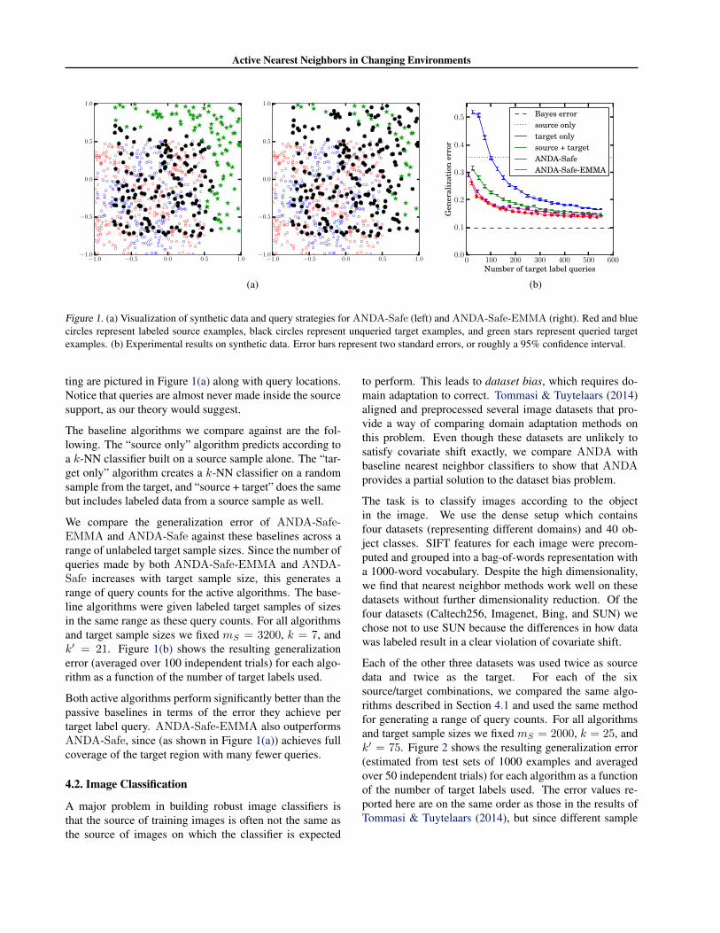
Figure 1. (a) Visualization of synthetic data and query strategies for ANDA-Safe (left) and ANDA-Safe-EMMA (right). Red and bluecircles represent labeled source examples, black circles represent unqueried target examples, and green stars represent queried targetexamples. (b) Experimental results on synthetic data. Error bars represent two standard errors, or roughly a 95% confidence interval.

ting are pictured in Figure 1(a) along with query locations.Notice that queries are almost never made inside the sourcesupport, as our theory would suggest.

The baseline algorithms we compare against are the fol-lowing. The “source only” algorithm predicts according toa k-NN classifier built on a source sample alone. The “tar-get only” algorithm creates a k-NN classifier on a randomsample from the target, and “source + target” does the samebut includes labeled data from a source sample as well.

We compare the generalization error of ANDA-Safe-EMMA and ANDA-Safe against these baselines across arange of unlabeled target sample sizes. Since the number ofqueries made by both ANDA-Safe-EMMA and ANDA-Safe increases with target sample size, this generates arange of query counts for the active algorithms. The base-line algorithms were given labeled target samples of sizesin the same range as these query counts. For all algorithmsand target sample sizes we fixed mS = 3200, k = 7, andk′ = 21. Figure 1(b) shows the resulting generalizationerror (averaged over 100 independent trials) for each algo-rithm as a function of the number of target labels used.

Both active algorithms perform significantly better than thepassive baselines in terms of the error they achieve pertarget label query. ANDA-Safe-EMMA also outperformsANDA-Safe, since (as shown in Figure 1(a)) achieves fullcoverage of the target region with many fewer queries.

4.2. Image Classification

A major problem in building robust image classifiers isthat the source of training images is often not the same asthe source of images on which the classifier is expected

to perform. This leads to dataset bias, which requires do-main adaptation to correct. Tommasi & Tuytelaars (2014)aligned and preprocessed several image datasets that pro-vide a way of comparing domain adaptation methods onthis problem. Even though these datasets are unlikely tosatisfy covariate shift exactly, we compare ANDA withbaseline nearest neighbor classifiers to show that ANDAprovides a partial solution to the dataset bias problem.

The task is to classify images according to the objectin the image. We use the dense setup which containsfour datasets (representing different domains) and 40 ob-ject classes. SIFT features for each image were precom-puted and grouped into a bag-of-words representation witha 1000-word vocabulary. Despite the high dimensionality,we find that nearest neighbor methods work well on thesedatasets without further dimensionality reduction. Of thefour datasets (Caltech256, Imagenet, Bing, and SUN) wechose not to use SUN because the differences in how datawas labeled result in a clear violation of covariate shift.

Each of the other three datasets was used twice as sourcedata and twice as the target. For each of the sixsource/target combinations, we compared the same algo-rithms described in Section 4.1 and used the same methodfor generating a range of query counts. For all algorithmsand target sample sizes we fixed mS = 2000, k = 25, andk′ = 75. Figure 2 shows the resulting generalization error(estimated from test sets of 1000 examples and averagedover 50 independent trials) for each algorithm as a functionof the number of target labels used. The error values re-ported here are on the same order as those in the results ofTommasi & Tuytelaars (2014), but since different sample


0 50 100 150 200 250 300 350Number of target label queries

0.76

0.78

0.80

0.82

0.84

0.86

0.88

0.90

0.92

0.94

Gen

eral

izat

ion

erro

r

source onlytarget onlysource + targetANDA-SafeANDA-Safe-EMMA

(a) Imagenet→ Caltech256

0 200 400 600 800 1000 1200 1400 1600Number of target label queries

0.86

0.88

0.90

0.92

0.94

0.96

0.98

Gen

eral

izat

ion

erro

r


(b) Caltech256→ Imagenet


0.93

0.94

0.95

0.96

0.97

Gen

eral

izat

ion

erro

r


(c) Caltech256→ Bing

0 50 100 150 200 250 300 350Number of target label queries

0.75

0.80

0.85

0.90

0.95

Gen

eral

izat

ion

erro

r


(d) Bing→ Caltech256

0 200 400 600 800 1000 1200 1400 1600Number of target label queries

0.86

0.88

0.90

0.92

0.94

0.96

0.98

Gen

eral

izat

ion

erro

r


(e) Bing→ Imagenet


0.91

0.92

0.93

0.94

0.95

0.96

0.97

0.98

Gen

eral

izat

ion

erro

r


(f) Imagenet→ Bing

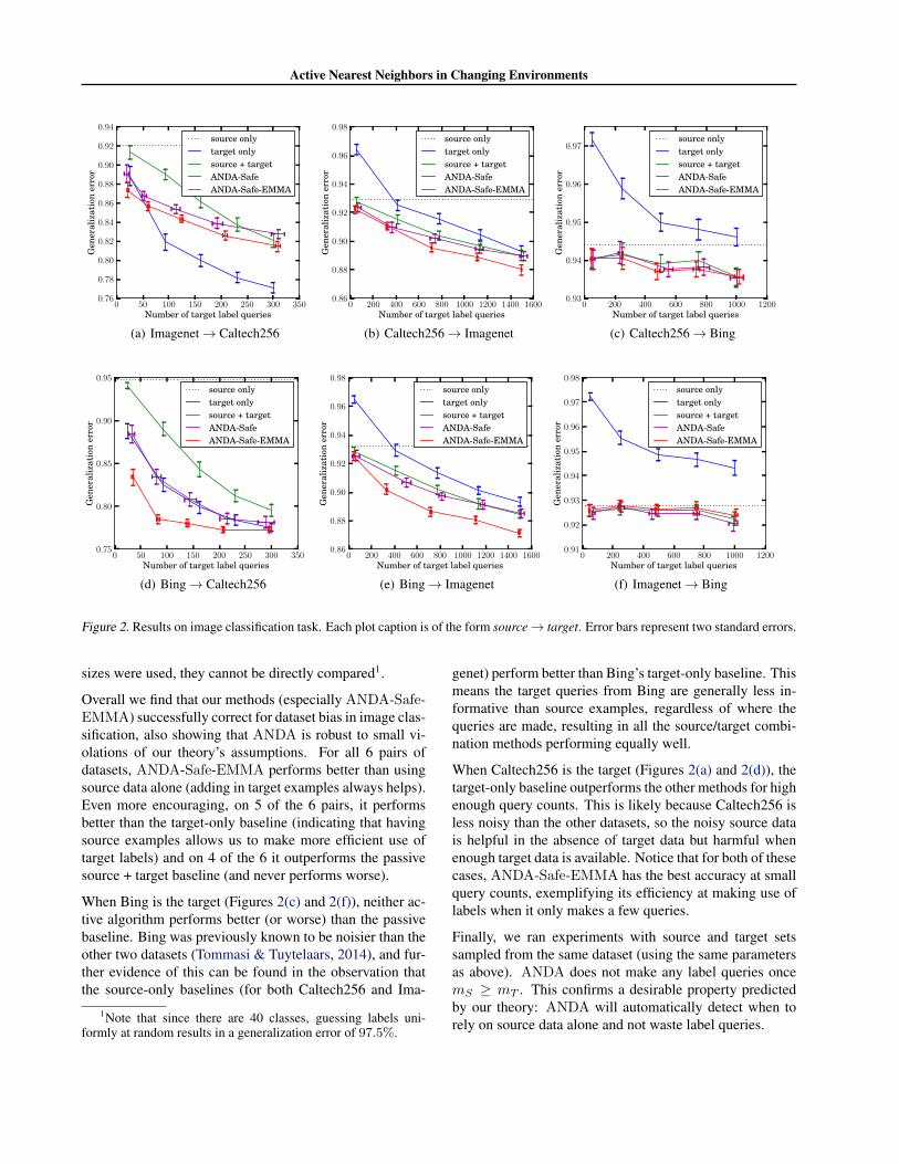
Figure 2. Results on image classification task. Each plot caption is of the form source→ target. Error bars represent two standard errors.

sizes were used, they cannot be directly compared1.

Overall we find that our methods (especially ANDA-Safe-EMMA) successfully correct for dataset bias in image clas-sification, also showing that ANDA is robust to small vi-olations of our theory’s assumptions. For all 6 pairs ofdatasets, ANDA-Safe-EMMA performs better than usingsource data alone (adding in target examples always helps).Even more encouraging, on 5 of the 6 pairs, it performsbetter than the target-only baseline (indicating that havingsource examples allows us to make more efficient use oftarget labels) and on 4 of the 6 it outperforms the passivesource + target baseline (and never performs worse).

When Bing is the target (Figures 2(c) and 2(f)), neither ac-tive algorithm performs better (or worse) than the passivebaseline. Bing was previously known to be noisier than theother two datasets (Tommasi & Tuytelaars, 2014), and fur-ther evidence of this can be found in the observation thatthe source-only baselines (for both Caltech256 and Ima-

1Note that since there are 40 classes, guessing labels uni-formly at random results in a generalization error of 97.5%.

genet) perform better than Bing’s target-only baseline. Thismeans the target queries from Bing are generally less in-formative than source examples, regardless of where thequeries are made, resulting in all the source/target combi-nation methods performing equally well.

When Caltech256 is the target (Figures 2(a) and 2(d)), thetarget-only baseline outperforms the other methods for highenough query counts. This is likely because Caltech256 isless noisy than the other datasets, so the noisy source datais helpful in the absence of target data but harmful whenenough target data is available. Notice that for both of thesecases, ANDA-Safe-EMMA has the best accuracy at smallquery counts, exemplifying its efficiency at making use oflabels when it only makes a few queries.

Finally, we ran experiments with source and target setssampled from the same dataset (using the same parametersas above). ANDA does not make any label queries oncemS ≥ mT . This confirms a desirable property predictedby our theory: ANDA will automatically detect when torely on source data alone and not waste label queries.


Acknowledgments

We would like to thank Nina Balcan for her vision andinspiration and for her support throughout the course ofthis project. Parts of this work were done while the sec-ond author was a postdoctoral fellow at Georgia Institute ofTechnology and at Carnegie Mellon University. This workwas supported in part by NSF grants CCF-1451177, CCF-1101283, CCF-1422910, ONR grant N00014-09-1-0751,AFOSR grant FA9550-09-1-0538, and a Microsoft FacultyFellowship.

ReferencesBalcan, Maria-Florina, Broder, Andrei, and Zhang, Tong.

Margin-based active learning. In COLT, 2007.

Balcan, Maria-Florina, Beygelzimer, Alina, and Langford,John. Agnostic active learning. J. Comput. Syst. Sci., 75(1), 2009.

Ben-David, Shai and Urner, Ruth. Domain adaptation-canquantity compensate for quality? Ann. Math. Artif. In-tell., 70(3):185–202, 2014.

Ben-David, Shai, Blitzer, John, Crammer, Koby, andPereira, Fernando. Analysis of representations for do-main adaptation. In NIPS, 2006.

Chattopadhyay, Rita, Fan, Wei, Davidson, Ian, Pan-chanathan, Sethuraman, and Ye, Jieping. Joint transferand batch-mode active learning. In ICML, 2013a.

Chattopadhyay, Rita, Wang, Zheng, Fan, Wei, Davidson,Ian, Panchanathan, Sethuraman, and Ye, Jieping. Batchmode active sampling based on marginal probability dis-tribution matching. TKDD, 7(3):13, 2013b.

Chaudhuri, Kamalika and Dasgupta, Sanjoy. Rates of con-vergence for nearest neighbor classification. In Advancesin Neural Information Processing Systems, pp. 3437–3445, 2014.

Cortes, Corinna, Mansour, Yishay, and Mohri, Mehryar.Learning bounds for importance weighting. In NIPS,2010.

Cover, Thomas M. and Hart, Peter E. Nearest neighborpattern classification. IEEE Transactions on InformationTheory, 13(1):21–27, 1967.

Dasgupta, Sanjoy. Analysis of a greedy active learningstrategy. In NIPS, 2004.

Dasgupta, Sanjoy. Two faces of active learning. Theor.Comput. Sci., 412(19):1767–1781, 2011.

Dasgupta, Sanjoy. Consistency of nearest neighbor classi-fication under selective sampling. In COLT, 2012.

Dasgupta, Sanjoy and Sinha, Kaushik. Randomized parti-tion trees for exact nearest neighbor search. In COLT,2013.

Hanneke, Steve. Rates of convergence in active learning.The Annals of Statistics, 39(1):333–361, 2011.

Kpotufe, Samory. k-NN regression adapts to local intrinsicdimension. In NIPS, 2011.

Kulkarni, Sanjeev R. and Posner, S. E. Rates of con-vergence of nearest neighbor estimation under arbitrarysampling. IEEE Transactions on Information Theory, 41(4):1028–1039, 1995.

Mansour, Yishay, Mohri, Mehryar, and Rostamizadeh, Af-shin. Domain adaptation: Learning bounds and algo-rithms. In COLT, 2009.

Pan, Sinno Jialin and Yang, Qiang. A survey on transferlearning. IEEE Transactions on Knowledge and DataEngineering, 22(10):1345–1359, October 2010. ISSN1041-4347.

Rajagopalan, Sridhar and Vazirani, Vijay V. Primal-dualRNC approximation algorithms for (multi)-set (multi)-cover and covering integer programs. In FOCS, 1993.

Ram, Parikshit and Gray, Alexander G. Which space parti-tioning tree to use for search? In NIPS, 2013.

Ram, Parikshit, Lee, Dongryeol, and Gray, Alexander G.Nearest-neighbor search on a time budget via max-margin trees. In SDM, 2012.

Saha, Avishek, Rai, Piyush, III, Hal Daume, Venkatasubra-manian, Suresh, and DuVall, Scott L. Active superviseddomain adaptation. In ECML/PKDD, 2011.

Settles, Burr. Active learning literature survey. Universityof Wisconsin, Madison, 52:55–66, 2010.

Shalev-Shwartz, Shai and Ben-David, Shai. UnderstandingMachine Learning. Cambridge University Press, 2014.

Shi, Yuan and Sha, Fei. Information-theoretical learning ofdiscriminative clusters for unsupervised domain adapta-tion. In ICML, 2012.

Stone, Charles J. Consistent nonparametric regression. TheAnnals of Statistics, 5(4):595–620, 07 1977.

Sugiyama, Masashi, Suzuki, Taiji, Nakajima, Shinichi,Kashima, Hisashi, von Bunau, Paul, and Kawanabe, Mo-toaki. Direct importance estimation for covariate shiftadaptation. Annals of the Institute of Statistical Mathe-matics, 60(4):699–746, 2008.


Tommasi, Tatiana and Tuytelaars, Tinne. A testbed forcross-dataset analysis. In TASK-CV Workshop at ECCV,2014.

Vapnik, Vladimir N. and Chervonenkis, Alexey J. On theuniform convergence of relative frequencies of events totheir probabilities. Theory of Probability & Its Applica-tions, 16(2):264–280, 1971.

Vazirani, Vijay. Approximation Algorithms. Springer,2001.

Zhao, Yingchao and Teng, Shang-Hua. Combinatorial andspectral aspects of nearest neighbor graphs in doublingdimensional and nearly-euclidean spaces. In TAMC,2007.

Active Nearest Neighbors in Changing Environments

Documents

Transcript of Active Nearest Neighbors in Changing Environments