A Bayesian reassessment of nearest-neighbour classification

A Bayesian reassessment of nearest-neighbour

classification

Lionel Cucala, Jean-Michel Marin, Christian Robert, Mike Titterington

To cite this version:

Lionel Cucala, Jean-Michel Marin, Christian Robert, Mike Titterington. A Bayesian reassess-ment of nearest-neighbour classification. [Research Report] RR-6173, INRIA. 2008. <inria-00143783v4>

HAL Id: inria-00143783

https://hal.inria.fr/inria-00143783v4

Submitted on 3 Mar 2008

HAL is a multi-disciplinary open accessarchive for the deposit and dissemination of sci-entific research documents, whether they are pub-lished or not. The documents may come fromteaching and research institutions in France orabroad, or from public or private research centers.

L’archive ouverte pluridisciplinaire HAL, estdestinee au depot et a la diffusion de documentsscientifiques de niveau recherche, publies ou non,emanant des etablissements d’enseignement et derecherche francais ou etrangers, des laboratoirespublics ou prives.

https://hal.archives-ouvertes.fr

https://hal.inria.fr/inria-00143783v4

appor t de r ech er ch e

ISS

N02

49-6

399

ISR

NIN

RIA

/RR

--61

73--

FR+E

NG

Thème COG

INSTITUT NATIONAL DE RECHERCHE EN INFORMATIQUE ET EN AUTOMATIQUE

A Bayesian reassessment of nearest–neighbourclassification

Lionel Cucala — Jean-Michel Marin — Christian P. Robert — Mike Titteringtion

N° 6173

January 2008

Unité de recherche INRIA FutursParc Club Orsay Université, ZAC des Vignes,

4, rue Jacques Monod, 91893 ORSAY Cedex (France)Téléphone : +33 1 72 92 59 00 — Télécopie : +33 1 60 19 66 08

A Bayesian reassessment of nearest–neighbour classification

Lionel Cucala∗ , Jean-Michel Marin† , Christian P. Robert ‡ , Mike Titteringtion §

Theme COG — Systemes cognitifsProjets select

Rapport de recherche n° 6173 — January 2008 — 20 pages

Abstract: The k-nearest-neighbour procedure is a well-known deterministic method used in supervisedclassification. This paper proposes a reassessment of this approach as a statistical technique derived from aproper probabilistic model; in particular, we modify the assessment made in a previous analysis of this methodundertaken by Holmes and Adams (2002, 2003), and evaluated by Manocha and Girolami (2007), where theunderlying probabilistic model is not completely well-defined. Once a clear probabilistic basis for the k-nearest-neighbour procedure is established, we derive computational tools for conducting Bayesian inference on theparameters of the corresponding model. In particular, we assess the difficulties inherent to pseudo-likelihoodand to path sampling approximations of an intractable normalising constant, and propose a perfect samplingstrategy to implement a correct MCMC sampler associated with our model. If perfect sampling is not avail-able, we suggest using a Gibbs sampling approximation. Illustrations of the performance of the correspondingBayesian classifier are provided for several benchmark datasets, demonstrating in particular the limitations ofthe pseudo-likelihood approximation in this set-up.

Key-words: Bayesian inference, classification, compatible conditionals, Boltzmann model, normalising con-stant, pseudo-likelihood, path sampling, perfect sampling, MCMC algorithms

∗ INRIA Saclay, Projet select, Universite Paris-Sud† INRIA Salclay, Projet select, Universite Paris-Sud and CREST, INSEE‡ CEREMADE, Universite Paris Dauphine and CREST, INSEE§ University of Glasgow

Reformulation bayesienne de la methode des k-plus-proches-voisins

Resume : Bien que maintenant supplantee par des methodes plus recentes, l’heuristique des k-plus-proches-voisins reste essentielle en classification supervisee. Dans cet article, nous en proposons une reformulation sousforme d’une modele statistique. Nous corrigeons ainsi les reformulations effectuees par Holmes and Adams(2002, 2003) pour lesquelles le modele sous-jacent n’est pas proprement defini. Le modele propose dependd’une constante de normalisation inconnue. Nous nous placons dans le paradigme bayesien et comparonsdifferentes methodes d’inference palliant cette difficulte. Nous etudions les limites de l’utilisation de la pseudo-vraisemblance et de la methode d’Ogata (Ogata, 1989) dans un schema MCMC et proposons une methodeMCMC exacte basee sur la simulation parfaite par couplage. Lorsque l’on ne peut pas utiliser la technique dela simulation parfaite ou si celle-ci s’avere trop couteuse, nous proposons de la remplacer par la methode del’echantillonnage de Gibbs. Nous illustrons les performances de cet algorithme sur divers jeu de donnees.

Mots-cles : Inference bayesienne, classification, lois conditionnelles compatibles, modele de Boltzmann,constante de normalisation, pseudo-vraisemblance, methode d’Ogata, simulation parfaite par couplage, algo-rithmes MCMC

Bayesian supervised classification 3

1 Introduction

1.1 Deterministic versus statistical classification

Supervised classification has long been used in both Machine Learning and Statistics to infer about the func-tional connection between a group of covariates (or explanatory variables) and a vector of indicators (or classes)(see, e.g., McLachlan, 1992; Ripley, 1994, 1996; Devroye et al., 1996; Hastie et al., 2001). For instance, themethod of boosting (Freund and Schapire, 1997) has been developed for this very purpose by the MachineLearning community and has also been assessed and extended by statisticians (Hastie et al., 2001; Buhlmannand Yu, 2002, 2003; Buhlmann, 2004; Zhang and Yu, 2005).

The k-nearest-neighbour method is a well-established and straightforward technique in this area with botha long past and a fairly resilient resistance to change (Ripley, 1994, 1996). Nonetheless, while providing aninstrument for classifying points into two or more classes, it lacks a corresponding assessment of its classificationerror. While alternative techniques like boosting offer this assessment, it is obviously of interest to provide theoriginal k-nearest-neighbour method with this additional feature. In contrast, statistical classification methodsthat are based on a model such a mixture of distributions do provide an assessment of error along with themost likely classification. This more global perspective thus requires the technique to be embedded within aprobabilistic framework in order to give a proper meaning to the notion of classification error. Holmes andAdams (2002) propose a Bayesian analysis of the k-nearest-neighbour-method based on these premises, and werefer the reader to this paper for background and references. In a separate paper, Holmes and Adams (2003)defined another model based on autologistic representations and conducted a likelihood analysis of this model, inparticular for selecting the value of k. While we also adopt a Bayesian approach, our paper differs from Holmesand Adams (2002) in two important respects: first, we define a global probabilistic model that encapsulatesthe k-nearest-neighbour method, rather than working with incompatible conditional distributions, and, second,we derive a fully operational simulation technique adapted to our model and based either on perfect samplingor on a Gibbs sampling approximation, that allows for a reassessment of the pseudo-likelihood approximationoften used in those settings.

1.2 The original k-nearest-neighbour method

Given a training set of individuals allocated each to one of G classes, the classical k-nearest-neighbour procedureis a method that allocates new individuals to the most common class in their neighbourhood among the trainingset, the neighbourhood being defined in terms of the covariates. More formally, based on a training dataset((yi, xi))

ni=1 , where yi ∈ {1, . . . , G} denotes the class label of the ith point and xi ∈ Rp is a vector of covariates,

an unobserved class yn+1 associated with a new set of covariates xn+1 is estimated by the most common classamong the k nearest neighbours of xn+1 in the training set (xi)

ni=1. The neighbourhood is defined in the space

of the covariates xi, namely

N kn+1 =

{1 ≤ i ≤ n; d(xi, xn+1) ≤ d(·, xn+1)(k)

},

where d(·, xn+1) denotes the vector of distances to xn+1 and d(·, xn+1)(k) denotes the kth order statistic. Theoriginal k-nearest-neighbour method usually uses the Euclidean norm, even though the Mahalanobis distancewould be more appropriate in that it rescales the covariates. Whenever ties occur, they are resolved bydecreasing the number k of neighbours until the problem disappears. When some covariates are categorical,other types of distance can be used instead, as in the R package knncat of Buttrey (1998).

As such, and as also noted in Holmes and Adams (2002), the method is both deterministic, given thetraining dataset, and not parameterised, even though the choice of k is both non-trivial and relevant to theperformance of the method. Usually, k is selected via cross-validation, as the number of neighbours thatminimises the cross-validation error rate. In contrast to cluster-analysis set-ups, the number G of classes inthe k-nearest-neighbour procedure is fixed and given by the training set: the introduction of additional classesthat are not observed in the training set has no effect on the future allocations.

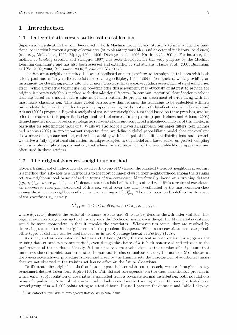
To illustrate the original method and to compare it later with our approach, we use throughout a toybenchmark dataset taken from Ripley (1994). This dataset corresponds to a two-class classification problem inwhich each (sub)population of covariates is simulated from a bivariate normal distribution, both populationsbeing of equal sizes. A sample of n = 250 individuals is used as the training set and the model is tested on asecond group of m = 1, 000 points acting as a test dataset. Figure 1 presents the dataset1 and Table 1 displays

1This dataset is available at http://www.stats.ox.ac.uk/pub/PRNN.

RR n° 6173

4 Cucala & Marin & Robert & Titterington

●●

●

●

●

●

●

●

●

●●●

●●

●

●

●●

●

●

●

● ●●

●●

●

●

●

●

●

●

●

●

●

●

●

●

●

●

●●

●●

●

●

●

●

●

●

●●

●

●

●

●

●

●

●

●

●

●

●

●●

●

●

●

●

●

●

●

●

●

●

●

●

●

●●

●

●

●

●

●

●●

●

●

●

●●

●

●

●

●

●

● ●●●

● ●●

●

●●

●

●

●

●

●

●

●

●

●

●

●●

●

●

●

●

●●

●

●

●

●●

●

●

●●

●

● ●

●

●●

●●

●

●

●

●

●

●

●

● ●

●●● ●

●●

●

●

●

●

●

●

●

●

●

●

●

●

●

●●●

●●

●●

●

●●

●●

●

●

●

●

●

●

●

●●●

●●

●● ●●

●●

●●

●

●

●

●●

●

●

●

●

●

● ●

●

●

●

●

●

●●

●●

●

●

●

● ●

●

●

●

●

●●

●

●

●

●●

●

●

●

●

●

●●

●

●

●

●

−1.0 −0.5 0.0 0.5 1.0

−0.

20.

20.

61.

0

●

●

●

●●

●

●

●●

●

● ●

●

●●

●●

●

●

●

●

●

●

●

● ●

●●● ●

●●

●

●

●

●

●

●

●

●

●

●

●

●

●

●●●

●●

●●

●

●●

●●

●

●

●

●

●

●

●

●●●

●●

●● ●●

●●

●●

●

●

●

●●

●

●

●

●

●

● ●

●

●

●

●

●

●●

●●

●

●

●

● ●

●

●

●

●

●●

●

●

●

●●

●

●

●

●

●

●●

●

●

●

●

●

●

●

●

●

●

●

●

●

●

●

●

●

●

●●

●

●●

●

●

●

●●●

●●●

●

●

● ●●●

●

●●

●●

●

●●

●●●

●

●

●

●

●

●

● ●●

●●

●

●

●●

●●

●●● ●

●

●

●

●

●

● ●

●

●

●

●

●●

●

●● ●

●●●

●

● ●

●●

●

●●

●●

●

●

●

●

●

●●

●

●

●

●

●

●●

●●

●

●

● ● ●

●

●

●

●

●

●

●

●

●

●

●

●

●

●

●

●

●●

●

●

● ●

●

●

●

●● ●

●

●

●

●

● ●●

●●

●

●

●

●

●

● ●

●

●

●

●

●● ●●

●●

●

● ●

●

●

●●

●

●

●

●●

●●

●

●

●

●

●

●●

●●●

●

●

●●

●

●

●

●

●●

●●

●

● ●

●

●

●

●

●

●

●

●

●

●

●

●●

●

●

● ●

●

●

●

●

●

●●

●

●●

●●

●

● ●●●

●

●

●

●

●● ●

● ●

●

●

●

● ●

●

●

●

●

●

● ●●

●

●

●●

●

●

●

●

●

●

●

●

●

●

●

●●

●

●

●

●

●

●

●

●●

●●

●●●

●

●●

●

●●

●

●●●

●

●

●

●

●

● ●

●

●

●

●

●

●

●

●

●

●

●

●●

●

●

●

●●●

●

●

●

●

●

●

●

●

●●●

●

●

●

●●

●

●

●

●

●

●

●

●●

●

●

●

●●

●

●

●

●●●

●

● ●

●●

●

●

●

● ●

●

●

●

●

●

●

●

●

●

●

●

●●

● ●●

●

●

●●●

●●●

●●

●

●●

●

●

●

●

●

● ●

●

●

●

●

●

●

●● ●

●

●

●

●

●

●

●●

●

●●

●

●

●●

●

●

●

●

●

●●●

●●

●

●●

●

●

●● ●

●

●

●

●

●

●●●

●

●● ●●

●

●

●

●●

●

●

●

●●

● ●

●●

●●

●

●

●

●●

●

●

●

●●

●

● ●

●

● ●●

●

●●

●

●

● ●

●

● ●●

●

●

●

●

●●

●●

●

●

●●

●

●

● ●

●

●

●

●

●●

●

●●

●

●

●

●

●

●

●

●

●

●

●

●

●●

●●

● ● ●

●

●

●●

●

●

●

●

● ● ●●

●

●●

●

●

●

●

●●

● ●

●

●

●

●

●

●

●

● ●

●●

●

●

●

● ●

●●

●●

●

●

●●

●

●

●

●

●

●

●

●

●

●

●●

●

●

●

●●

●

●

●

●●

●

●

●

●

●

●

●

●

●

●

●

●●

●

●●

●

●

●

● ●

●

●

●

●

●

●

●

●●

●

●●

●

●

●

●

●

●

●

●●

●●

●●

● ●●

●●

●●●

●● ●

●

●

●

●

●

●

●

●

●

●●

●

●

●●

●

●

●

●

●●

●

●●●

●●

●

●

●

●

●

● ●●

●

●

●●

●

●

●

●

●●●

●

●

●

● ●●

●

●●

●●

●

●

●

●

●

●

●

●● ●

●

●

●●

●

●

●

●

●

●●

●

●●

●

●

●

●

●

●

●●●

●●●

●

●

●

●

●

●

●

●

●

● ●

● ●

●

●

●●

●

●

●

●

●

●

●●

●●

●

●

●

●●

● ●

●●

●●

●

●

●

●

●

●

●●

●

●

●

●

●●

●

●

●

●

●●

●

● ●

●

●

●

●

●

●

● ●● ●

●

●●

●

●

●●

●

● ●

●

● ●● ●

●

●

●●

●

●

●

●

●

●●

● ●

●

●

●

●

● ●●●

●

●●

●●●

●

●

●

●

●

●

●

●

●

●

● ●

●●●

●●

● ●●

● ●

●

●

●

●

●

●

●

●

● ●

●●

●

●●

●

●

●

●

●

●

●

●

●

●

●

●●

●

●

●

●

●

●●

●●

●

●●

●

●●

●

●

●

●●●

●

●

●

●

●●

●

●●

●

●●

●● ●

●

●●

●●

●

●

●

●

●●

●●●●

●

●●

●

●

●

●

●

●

−1.0 −0.5 0.0 0.5 1.0

−0.

20.

20.

61.

0● ●

●

●

●●

●

●

● ●

●

● ●●

●

●

●

●

●●

●●

●

●

●●

●

●

● ●

●

●

●

●

●●

●

●●

●

●

●

●

●

●

●

●

●

●

●

●

●●

●●

● ● ●

●

●

●●

●

●

●

●

● ● ●●

●

●●

●

●

●

●

●●

● ●

●

●

●

●

●

●

●

● ●

●●

●

●

●

● ●

●●

●●

●

●

●●

●

●

●

●

●

●

●

●

●

●

●●

●

●

●

●●

●

●

●

●●

●

●

●

●

●

●

●

●

●

●

●

●●

●

●●

●

●

●

● ●

●

●

●

●

●

●

●

●●

●

●●

●

●

●

●

●

●

●

●●

●●

●●

● ●●

●●

●●●

●● ●

●

●

●

●

●

●

●

●

●

●●

●

●

●●

●

●

●

●

●●

●

●●●

●●

●

●

●

●

●

● ●●

●

●

●●

●

●

●

●

●●●

●

●

●

● ●●

●

●●

●●

●

●

●

●

●

●

●

●● ●

●

●

●●

●

●

●

●

●

●●

●

●●

●

●

●

●

●

●

●●●

●●●

●

●

●

●

●

●

●

●

●

● ●

● ●

●

●

●●

●

●

●

●

●

●

●●

●●

●

●

●

●●

● ●

●●

●●

●

●

●

●

●

●

●●

●

●

●

●

●●

●

●

●

●

●●

●

● ●

●

●

●

●

●

●

● ●● ●

●

●●

●

●

●●

●

● ●

●

● ●● ●

●

●

●●

●

●

●

●

●

●●

● ●

●

●

●

●

● ●●●

●

●●

●●●

●

●

●

●

●

●

●

●

●

●

● ●

●●●

●●

● ●●

● ●

●

●

●

●

●

●

●

●

● ●

●●

●

●●

●

●

●

●

●

●

●

●

●

●

●

●●

●

●

●

●

●

●●

●●

●

●●

●

●●

●

●

●

●●●

●

●

●

●

●●

●

●●

●

●●

●● ●

●

●●

●●

●

●

●

●

●●

●●●●

●

●●

●

●

●

●

●

●

Figure 1: Training (top) and test (bottom) groups for Ripley’s benchmark: the points in red are those for whichthe label is equal to 1 and the points in black are those for which the label is equal to 2.

the performance of the standard k-nearest-neighbour method on the test dataset for several values of k. Theoverall misclassification leave-one-out error rate on the training dataset as k varies is provided in Figure 2 andit shows that this criterion is not very discriminating for this dataset, with little variation for a wide range ofvalues of k and with several values of k achieving the same overall minimum, namely 17, 18, 35, 36, 45, 46, 51,52, 53 and 54. There are therefore ten different values of k in competition. This range of values is an indicatorof potential gains when averaging over k, and hence calls for a Bayesian perspective.

k Misclassificationerror rate

1 0.1503 0.13415 0.09517 0.08731 0.08454 0.081

Table 1: k-nearest-neighbour performances on the Ripley test dataset

0 20 40 60 80 100 120

3040

5060

k

Leav

e−on

e−ou

t cro

ss v

alid

atio

n er

ror

rate

Figure 2: Misclassification leave-one-out error rate as a function of k for Ripley’s training dataset.

INRIA


1.3 Goal and plan

As presented above, the k-nearest-neighbour method is merely an allocation technique that does not accountfor uncertainty. In order to add this feature, we need to introduce a probabilistic framework that relatesthe class label yi to both the covariates xi and the class labels of the neighbours of xi. Not only does thisperspective provide more information about the variability of the classification, when compared with the pointestimate given by the original method, but it also takes advantage of the full (Bayesian) inferential machineryto introduce parameters that measure the strength of the influence of the neighbours, and to analyse the role ofthe variables, of the metric used, of the number k of neighbours, and of the number of classes towards achievinghigher efficiency. Once again, this statistical viewpoint was previously adopted by Holmes and Adams (2002,2003) and we follow suit in this paper, with a modification of their original model geared towards a coherentprobabilistic model, while providing new developments in computational model estimation.

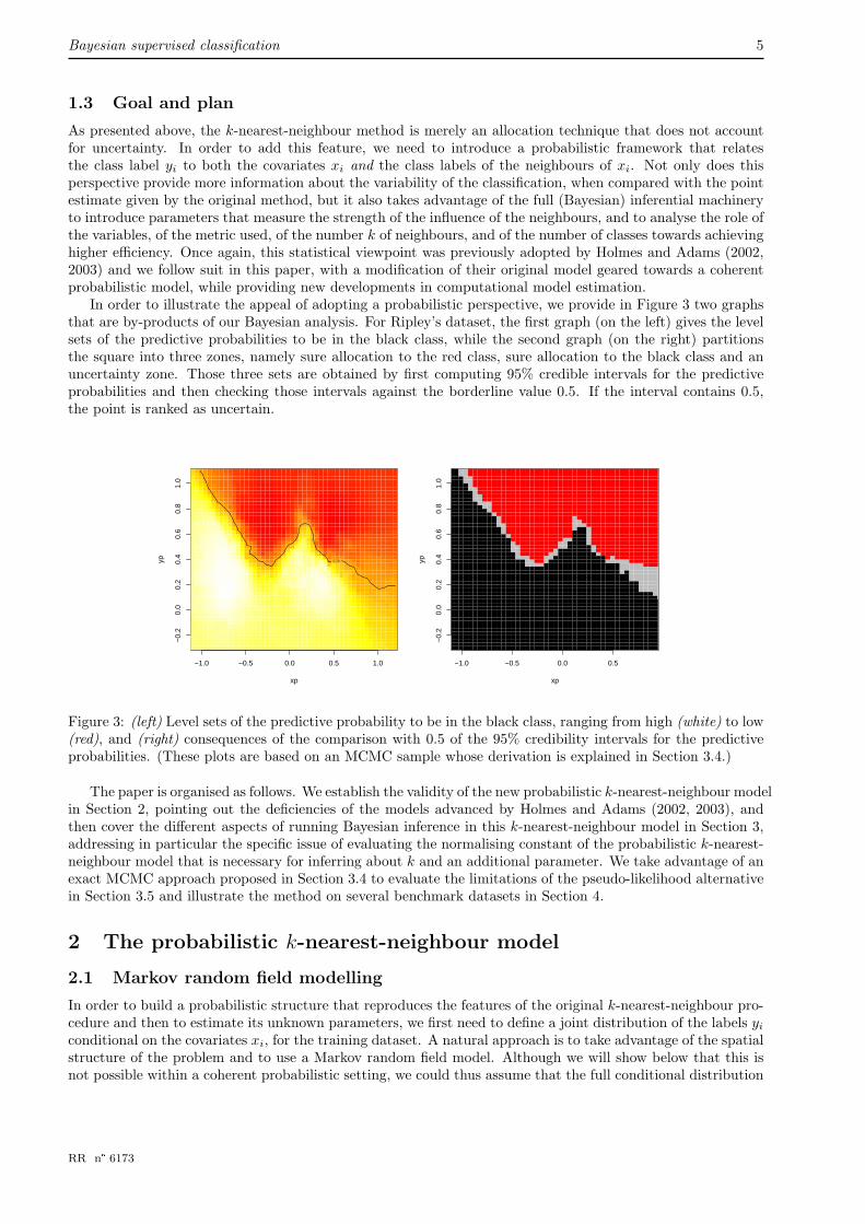
In order to illustrate the appeal of adopting a probabilistic perspective, we provide in Figure 3 two graphsthat are by-products of our Bayesian analysis. For Ripley’s dataset, the first graph (on the left) gives the levelsets of the predictive probabilities to be in the black class, while the second graph (on the right) partitionsthe square into three zones, namely sure allocation to the red class, sure allocation to the black class and anuncertainty zone. Those three sets are obtained by first computing 95% credible intervals for the predictiveprobabilities and then checking those intervals against the borderline value 0.5. If the interval contains 0.5,the point is ranked as uncertain.

−1.0 −0.5 0.0 0.5 1.0

−0.

20.

00.

20.

40.

60.

81.

0

xp

yp

−1.0 −0.5 0.0 0.5

−0.

20.

00.

20.

40.

60.

81.

0

xp

yp

Figure 3: (left) Level sets of the predictive probability to be in the black class, ranging from high (white) to low(red), and (right) consequences of the comparison with 0.5 of the 95% credibility intervals for the predictiveprobabilities. (These plots are based on an MCMC sample whose derivation is explained in Section 3.4.)

The paper is organised as follows. We establish the validity of the new probabilistic k-nearest-neighbour modelin Section 2, pointing out the deficiencies of the models advanced by Holmes and Adams (2002, 2003), andthen cover the different aspects of running Bayesian inference in this k-nearest-neighbour model in Section 3,addressing in particular the specific issue of evaluating the normalising constant of the probabilistic k-nearest-neighbour model that is necessary for inferring about k and an additional parameter. We take advantage of anexact MCMC approach proposed in Section 3.4 to evaluate the limitations of the pseudo-likelihood alternativein Section 3.5 and illustrate the method on several benchmark datasets in Section 4.

2 The probabilistic k-nearest-neighbour model

2.1 Markov random field modelling

In order to build a probabilistic structure that reproduces the features of the original k-nearest-neighbour pro-cedure and then to estimate its unknown parameters, we first need to define a joint distribution of the labels yiconditional on the covariates xi, for the training dataset. A natural approach is to take advantage of the spatialstructure of the problem and to use a Markov random field model. Although we will show below that this isnot possible within a coherent probabilistic setting, we could thus assume that the full conditional distribution

RR n° 6173


of yi given y−i = (y1, . . . , yi−1, yi+1, . . . , yn) and the xi’s only depends on the k nearest neighbours of xi inthe training set. The parameterised structure of this conditional distribution is obviously open but we opt forthe most standard choice, namely, like the Potts model, a Boltzmann distribution (Møller and Waagepetersen,2003) with potential function ∑

`∼ki

δyi(y`) ,

where ` ∼k i means that the summation is taken over the observations x` belonging to the k nearest neighboursof xi, and δa(b) denotes the Dirac function. This function actually gives the number of points from the sameclass yi as the point xi that are among the k nearest neighbours of xi. As in Holmes and Adams (2003), theexpression for the full conditional is thus

f(yi|y−i,X, β, k) = exp

(β∑`∼ki

δyi(y`)/k

)/G∑g=1

exp

(β∑`∼ki

δg(y`)/k

)(1)

where β > 0 and X is the (p, n) matrix {x1, . . . , xn} of coordinates for the training set.In this parameterised model, β is a quantity that is obviously missing from the original k-nearest-neighbour pro-

cedure. It is only relevant from a statistical point of view as a degree of uncertainty: β = 0 corresponds toa uniform distribution over all classes, meaning independence from the neighbours, while β = +∞ leads to apoint mass distribution at the prevalent class, corresponding to extreme dependence. The introduction of thescale parameter k in the denominator is useful in making β dimensionless.

There is, however, a difficulty with this expression in that, for almost all datasets X, there does not exista joint probability distribution on y = (y1, . . . , yn) with full conditionals equal to (1). This happens becausethe k-nearest-neighbour system is usually asymmetric: when xi is one of the k nearest neighbours of xj , xj isnot necessarily one of the k nearest neighbours of xi. Therefore, the pseudo-conditional distribution (1) willnot depend on xj while the equivalent for xj does depend on xi: this is obviously impossible in a coherentprobabilistic framework (Besag, 1974; Cressie, 1993)

One way of overcoming this fundamental difficulty is to follow Holmes and Adams (2002) and to definedirectly the joint distribution

f(y|X, β, k) =n∏i=1

exp

(β∑`∼ki

δyi(y`)

/k

)/G∑g=1

exp

(β∑`∼ki

δg(y`)/k

). (2)

Unfortunately, there are drawbacks to this approach, in that, first, the function (2) is not properly normalised(a fact overlooked by Holmes and Adams, 2002), and the necessary normalising constant is intractable. Second,the full conditional distributions corresponding to this joint distribution are not given by (1). The first drawbackis a common occurrence with Boltzmann models and we will deal with this difficulty in detail in Section 3.At this stage, let us point out that the most standard approach to this problem is to use pseudo-likelihoodfollowing Besag et al. (1991), as in Heikkinen and Hogmander (1994) and Hoeting et al. (1999), but we willshow in Section 3.5 that this approximation can give poor results. (See, e.g., Friel et al. (2005) for a discussionof this point.) The second and more specific drawback implies that (2) cannot be treated as a pseudo-likelihood(Besag, 1974; Besag et al., 1991)since, as stated above, the conditional distribution (1) cannot be associatedwith any joint distribution. That (2) misses a normalising constant can be seen from the special case in whichn = 2, y = (y1, y2) and G = 2, since

2∑y1=1

2∑y2=1

2∏i=1

exp

(β∑`∼ki

δyi(y`)/k

)/2∑g=1

exp

(β∑`∼ki

δg(y`)/k

)

=2∑

y1=1

2∑y2=1

exp (β [δy1(y2) + δy2(y1)] /k)

/(1 + eβ/k

)2

= 2(

1 + e2β/k)/(

1 + eβ/k)2

,

which is clearly different from 1 and, more importantly, depends on both β and k. We note that the debateabout whether or not one should use a proper joint distribution is reminiscent of the opposition betweenGaussian conditional autoregressions (CAR) and Gaussian intrinsic autoregressions in Besag and Kooperberg(1995), the latter not being associated with any joint distribution.

INRIA


2.2 A symmetrised Boltzmann modelling

Given these difficulties, we therefore adopt a different strategy and define a joint model on the training set as

f(y|X, β, k) = exp

(β

n∑i=1

∑`∼ki

δyi(y`)/k

)/Z(β, k) , (3)

where Z(β, k) is the normalising constant of the distribution. The motivation for this modelling is that thefull conditional distributions corresponding to (3) can be obtained as

f(yi|y−i,X, β, k) ∝ exp

{β/k

(∑`∼ki

δyi(y`) +

∑i∼k`

δy`(yi)

)}, (4)

where i ∼k ` means that the summation is taken over the observations x` for which xi is a k-nearest neighbour.Obviously, these conditional distributions differ from (1) if only because of the impossibility result mentionedabove. The additional term in the potential function corresponds to the observations that are not amongthe nearest neighbours of xi but for which xi is a nearest neighbour. In this model, compared with singleneighbours, mutual neighbours are given a double weight. This feature is of importance in that this coherentmodel defines a new classification criterion that can be treated as a competitor of the standard k-nearest-neighbour objective function. Note also that the original full conditional (1) is recovered as (4) when thesystem of neighbours is perfectly symmetric (up to a factor 2). Once again, the normalising constant Z(β, k)is intractable, except for the most trivial cases.

In the case of unbalanced sampling, that is, if the marginal probabilities p1 = P(y = 1), . . . , pG = P(y = G)are known and are different from the sampling probabilities p1 = n1/n, . . . , pG = nG/n, where ng is the numberof training observations arising from class g, a natural modification of this k-nearest-neighbour model is toreweight the neighbourhood sizes by ag = pgn/ng. This leads to the modified model

f(y|X, β, k) = exp

(β∑i

ayi

∑`∼ki

δyi(y`)/k

)/Z(β, k) .

This modification is useful in practice when we are dealing with stratified surveys. In the following, however,we assume that ag = 1 for all g = 1, . . . , G.

2.3 Predictive perspective

When based on the conditional expression (4), the predictive distribution of a new unclassified observationyn+1 given its covariate xn+1 and the training sample (y,X) is, for g = 1, . . . , G,

P(yn+1 = g|xn+1,y,X, β, k) ∝ exp

β/k ∑`∼k(n+1)

δg(y`) +∑

(n+1)∼k`

δy`(g)

, (5)

where ∑`∼k(n+1)

δg(y`) and∑

(n+1)∼k`

δy`(g)

are the numbers of observations in the training dataset from class g among the k nearest neighbours of xn+1

and among the observations for which xn+1 is a k-nearest neighbour, respectively. This predictive distributioncan then be incorporated in the Bayesian inference process by considering the joint posterior of (β, k, yn+1)and by deriving the corresponding marginal posterior distribution of yn+1.

While this model provides a sound statistical basis for the k-nearest-neighour methodology as well as a meansof assessing the uncertainty of the allocations to classes of unclassified observations, and while it corresponds toa true, albeit unavailable, joint distribution, it can be criticised from a Bayesian point of view in that it suffersfrom a lack of statistical coherence (in the sense that the information contained in the sample is not used in themost efficient way) when multiple classifications are considered. Indeed, the k-nearest-neighbour methodologyis invariably used in a repeated manner, either jointly on a sample (xn+1, . . . , xn+m) or sequentially. Ratherthan assuming simultaneously dependence in the training sample and independence in the unclassified sample,it would be more sensible to consider the whole collection of points as issuing from a single joint model of the

RR n° 6173


form given by (3), but with some having their class missing at random. Always reasoning from a Bayesian pointof view, addressing jointly the inference on the parameters (β, k) and on the missing classes (yn+1, . . . , yn+m)—i.e. assuming exchangeability between the training and the unclassified datapoints—certainly makes sense froma foundational perspective as a correct probabilistic evaluation and it does provide a better assessment of theuncertainty about the classifications as well as about the parameters.

Unfortunately, this more global and arguably more coherent perspective is mostly unachievable if only forcomputational reasons, since the set of the missing class vector (yn+1, . . . , yn+m) is of size Gm. It is practicallyimpossible to derive an efficient simulation algorithm that would correctly approximate the joint probabilitydistribution of both parameters and classes, especially when the number m of unclassified points is large. Wewill thus adopt the more ad hoc approach of dealing separately with each unclassified point in the analysis,because this simply is the only realistic way. This perspective can also be justified by the fact that, in realisticmachine learning set-ups, the unclassified data (yn+1, . . . , yn+m) mostly occur in a sequential environmentwith, furthermore, the true value of yn+1 being revealed before yn+2 is observed.

In the following sections, we mainly consider the case G = 2 as in Holmes and Adams (2003), becausethis is the only case where we can conduct a full comparison between different approximation schemes, but weindicate at the end of Section 3.4 how a Gibbs sampling approximation allows for a realistic extension to largervalues of G, as illustrated in Section 4.

3 Bayesian inference and the normalisation problem

Given the joint model (3) for (y1, . . . , yn+1), Bayesian inference can be conducted in a standard manner(Robert, 2001), provided computational difficulties related to the unavailability of the normalising constantcan be solved. Indeed, as stressed in the previous section, from a Bayesian perspective, the classification ofunclassified points can be based on the marginal predictive (or posterior) distribution of yn+1 obtained byintegration over the conditional posterior distribution of the parameters, namely, for g = 1, 2,

P(yn+1 = g|xn+1,y,X) =∑k

∫P(yn+1 = g|xn+1,y,X, β, k)π(β, k|y,X) dβ , (6)

where π(β, k|y,X) ∝ f(y|X, β, k)π(β, k) is the posterior distribution of (β, k) given the training dataset (y,X).While other choices of prior distributions are available, we choose for (k, β) a uniform prior on the compactsupport {1, . . . ,K}× [0, βmax ]. The limitation on k is imposed by the structure of the training dataset in thatK is at most equal to the minimal class size, min(n1, n2), while the limitation on β, β < βmax , is customaryin Boltzmann models, because of phase-transition phenomena (Møller, 2003): when β is above a certain value,the model becomes ”all black or all white”, i.e. all yi’s are either equal to 1 or to 2. (This is illustrated in Figure5 below by the convergence of the expectation of the number of identical neighbours to k.) The determinationof βmax is obviously problem-specific and needs to be solved afresh for each new dataset since it depends onthe topology of the neighbourhood. It is however straighforward to implement in that a Gibbs simulation of(3) for different values of β quickly exhibits the “black-or-white” features.

3.1 MCMC steps

Were the posterior distribution π(β, k|y,X) available (up to a normalising constant), we could design anMCMC algorithm that would produce a Markov chain approximating a sample from this posterior (Robertand Casella, 2004), for example through a Gibbs sampling scheme based on the full conditional distributions ofboth k and β. However, because of the associated representation (4), the conditional distribution of β is non-standard and we need to resort to a hybrid sampling scheme in which the exact simulation from π(β|k,y,X)is replaced with a single Metropolis–Hastings step. Furthermore, use of the full conditional distribution fork can impose fairly severe computational constraints. Indeed, for a given value β(t), computing the posteriorf(y|X, β(t), i)π(β(t), i), for i = 1, . . . ,K, requires computations of order O(KnG), once again because of thelikelihood representation. A faster alternative is to use a hybrid step for both β and k: in this way, we onlyneed to compute the full conditional distribution of k for one new value of k, modulo the normalising constant.

An alternative to Gibbs sampling is to use a random walk Metropolis–Hastings algorithm: both β and kare then updated using random walk proposals. Since β ∈ (0, βmax) is constrained, we first introduce a logisticreparameterisation of β,

β = βmax exp(θ)/

(exp(θ) + 1) ,

INRIA


and then propose a normal random walk on the θ’s, θ′ ∼ N (θ(t), τ2). For k, we use instead a uniformproposal on the 2r neighbours of k(t), namely {k(t) − r, . . . , k(t) − 1, k(t) + 1, . . . k(t) + r}

⋂{1, . . . ,K}. This

proposal distribution with probabiltity density Qr(k, ·), with k′ ∼ Qr(k(t−1), ·), thus depends on a parameterr ∈ {1, . . . ,K} that needs to be calibrated so as to aim at optimal acceptance rates, as does τ2. The acceptanceprobability in the Metropolis–Hastings algorithm is thus

ρ =f(y|X, β′, k′)π(β′, k′)

/Qr(k(t−1), k′)

f(y|X, β(t−1), k(t−1))π(β(t−1), k(t−1))/Qr(k′, k(t−1))

×exp(θ′)

/(1 + exp(θ′))2

exp(θ(t−1))/

(1 + exp(θ(t−1)))2,

where the second ratio is the ratio of the Jacobians due to the reparameterisation.Once the Metropolis–Hastings algorithm has produced a satisfactory sequence of (β, k)’s, the Bayesian

prediction for an unobserved class yn+1 associated with xn+1 is derived from (6). In fact, if we use a 0− 1 lossfunction (Robert, 2001) for predicting yn+1, namely

L(yn+1, yn+1) = Iyn+1 6=yn+1 ,

the Bayes estimator yπn+1 is the most probable class g according to the posterior predictive (6). The associatedmeasure of uncertainty is then the posterior expected loss, P(yn+1 = g|xn+1,y,X).

Explicit calculation of (6) is obviously impossible and this distribution must be approximated from theMCMC chain {(β, k)(1), . . . , (β, k)(M)} simulated above, namely by

M−1M∑i=1

P(yn+1 = g|xn+1,y,X, (β, k)(i)

). (7)

Unfortunately, since (3) involves the intractable constant Z(β, k), the above schemes cannot be implementedas such and we need to replace f with a more manageable target. We proceed below through three differentapproaches that try to overcome this difficulty, postponing the comparison till Section 3.5.

3.2 Pseudo-likelihood approximation

A first solution, dating back to Besag (1974), is to replace the true joint distribution with the pseudo-likelihood,defined as

f(y|X, β, k) =n∏i=1

exp

{β/k

(∑`∼ki

δyi(y`) +∑i∼k`

δy`(yi)

)}2∑g=1

exp

{β/k

(∑`∼ki

δg(y`) +∑i∼k`

δy`(g)

)} (8)

and made up of the product of the (true) conditional distributions associated with (3). The true posteriordistribution π(β, k|y,X) is then replaced with

π(β, k|y,X) ∝ f(y|X, β, k)π(β, k) ,

and used as such in all steps of the MCMC algorithm drafted above. The predictive distribution P(yn+1 =g|xn+1,y,X) is correspondingly approximated by (7), based on the pseudo-sample thus produced.

While this replacement of the true distribution with the pseudo-likelihood approximation induces a bias inthe estimation of (k, β) and in the predictive performance of the Bayes procedure, it has been intensively usedin the past, if only because of its availability and simplicity. For instance, Holmes and Adams (2003) built theirpseudo-joint distribution on such a product (with the difficulty that the components of the product were nottrue conditionals). As noted in Friel and Pettitt (2004), pseudo-likelihood estimation can be very misleadingand we will describe its performance in more detail in Section 3.5. (To the best of our knowledge, this Bayesianevaluation has not been conducted before.)

As illustrated on Figure 4 for Ripley’s benchmark data, the random walk Metropolis–Hastings algorithmdetailed above performs satisfactorily with the pseudo-likelihood approximation, even though the mixing is slow

RR n° 6173


0 10000 30000 50000

1.5

2.0

2.5

3.0

3.5

4.0

Fre

quen

cy

1.0 1.5 2.0 2.5 3.0 3.5

010

020

030

040

050

0

0 10000 30000 50000

2030

4050

6070

80

13 22 31 40 49 58 67 76

010

020

030

040

0

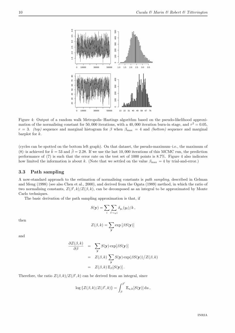
Figure 4: Output of a random walk Metropolis–Hastings algorithm based on the pseudo-likelihood approxi-mation of the normalising constant for 50, 000 iterations, with a 40, 000 iteration burn-in stage, and τ2 = 0.05,r = 3. (top) sequence and marginal histogram for β when βmax = 4 and (bottom) sequence and marginalbarplot for k.

(cycles can be spotted on the bottom left graph). On that dataset, the pseudo-maximum–i.e., the maximum of(8)–is achieved for k = 53 and β = 2.28. If we use the last 10, 000 iterations of this MCMC run, the predictionperformance of (7) is such that the error rate on the test set of 1000 points is 8.7%. Figure 4 also indicateshow limited the information is about k. (Note that we settled on the value βmax = 4 by trial-and-error.)

3.3 Path sampling

A now-standard approach to the estimation of normalising constants is path sampling, described in Gelmanand Meng (1998) (see also Chen et al., 2000), and derived from the Ogata (1989) method, in which the ratio oftwo normalising constants, Z(β′, k)/Z(β, k), can be decomposed as an integral to be approximated by MonteCarlo techniques.

The basic derivation of the path sampling approximation is that, if

S(y) =∑i

∑`∼ki

δyi(y`)/k ,

thenZ(β, k) =

∑y

exp [βS(y)]

and

∂Z(β, k)∂β

=∑y

S(y) exp[βS(y)]

= Z(β, k)∑y

S(y) exp(βS(y))/Z(β, k)

= Z(β, k) Eβ [S(y)] .

Therefore, the ratio Z(β, k)/Z(β′, k) can be derived from an integral, since

log {Z(β, k)/Z(β′, k)} =∫ β′

β

Eu,k[S(y)] du ,

INRIA


0 1 2 3 4

140

160

180

200

220

240

0 1 2 3 4

140

160

180

200

220

240

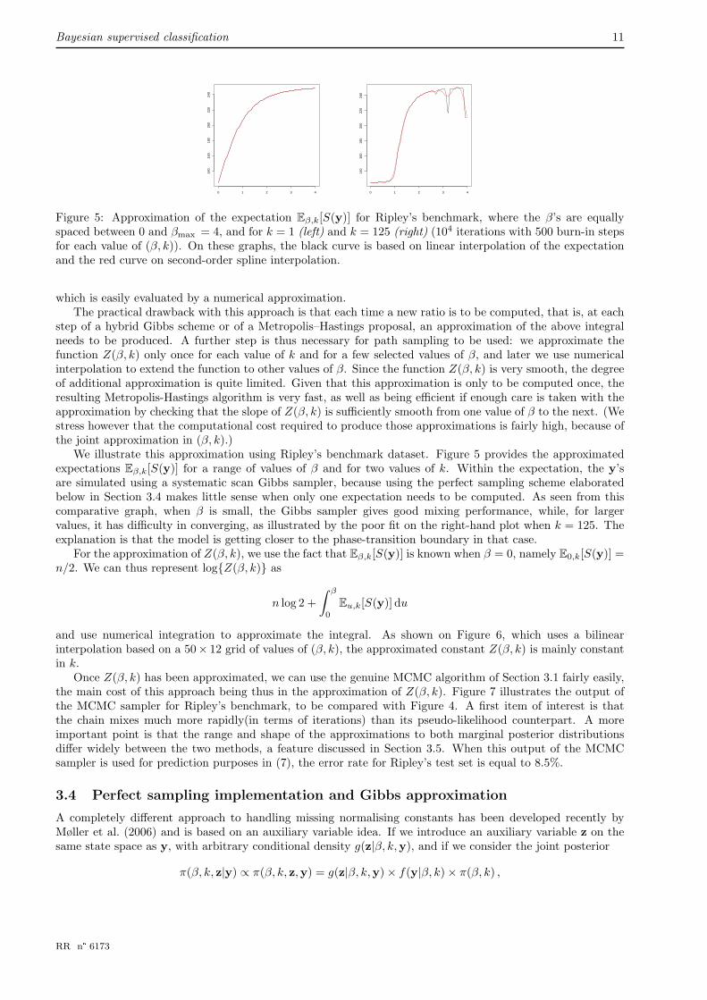
Figure 5: Approximation of the expectation Eβ,k[S(y)] for Ripley’s benchmark, where the β’s are equallyspaced between 0 and βmax = 4, and for k = 1 (left) and k = 125 (right) (104 iterations with 500 burn-in stepsfor each value of (β, k)). On these graphs, the black curve is based on linear interpolation of the expectationand the red curve on second-order spline interpolation.

which is easily evaluated by a numerical approximation.The practical drawback with this approach is that each time a new ratio is to be computed, that is, at each

step of a hybrid Gibbs scheme or of a Metropolis–Hastings proposal, an approximation of the above integralneeds to be produced. A further step is thus necessary for path sampling to be used: we approximate thefunction Z(β, k) only once for each value of k and for a few selected values of β, and later we use numericalinterpolation to extend the function to other values of β. Since the function Z(β, k) is very smooth, the degreeof additional approximation is quite limited. Given that this approximation is only to be computed once, theresulting Metropolis-Hastings algorithm is very fast, as well as being efficient if enough care is taken with theapproximation by checking that the slope of Z(β, k) is sufficiently smooth from one value of β to the next. (Westress however that the computational cost required to produce those approximations is fairly high, because ofthe joint approximation in (β, k).)

We illustrate this approximation using Ripley’s benchmark dataset. Figure 5 provides the approximatedexpectations Eβ,k[S(y)] for a range of values of β and for two values of k. Within the expectation, the y’sare simulated using a systematic scan Gibbs sampler, because using the perfect sampling scheme elaboratedbelow in Section 3.4 makes little sense when only one expectation needs to be computed. As seen from thiscomparative graph, when β is small, the Gibbs sampler gives good mixing performance, while, for largervalues, it has difficulty in converging, as illustrated by the poor fit on the right-hand plot when k = 125. Theexplanation is that the model is getting closer to the phase-transition boundary in that case.

For the approximation of Z(β, k), we use the fact that Eβ,k[S(y)] is known when β = 0, namely E0,k[S(y)] =n/2. We can thus represent log{Z(β, k)} as

n log 2 +∫ β

0

Eu,k[S(y)] du

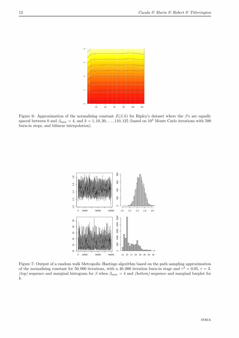
and use numerical integration to approximate the integral. As shown on Figure 6, which uses a bilinearinterpolation based on a 50× 12 grid of values of (β, k), the approximated constant Z(β, k) is mainly constantin k.

Once Z(β, k) has been approximated, we can use the genuine MCMC algorithm of Section 3.1 fairly easily,the main cost of this approach being thus in the approximation of Z(β, k). Figure 7 illustrates the output ofthe MCMC sampler for Ripley’s benchmark, to be compared with Figure 4. A first item of interest is thatthe chain mixes much more rapidly(in terms of iterations) than its pseudo-likelihood counterpart. A moreimportant point is that the range and shape of the approximations to both marginal posterior distributionsdiffer widely between the two methods, a feature discussed in Section 3.5. When this output of the MCMCsampler is used for prediction purposes in (7), the error rate for Ripley’s test set is equal to 8.5%.

3.4 Perfect sampling implementation and Gibbs approximation

A completely different approach to handling missing normalising constants has been developed recently byMøller et al. (2006) and is based on an auxiliary variable idea. If we introduce an auxiliary variable z on thesame state space as y, with arbitrary conditional density g(z|β, k,y), and if we consider the joint posterior

π(β, k, z|y) ∝ π(β, k, z,y) = g(z|β, k,y)× f(y|β, k)× π(β, k) ,

RR n° 6173


20 40 60 80 100 120

01

23

4

Figure 6: Approximation of the normalising constant Z(β, k) for Ripley’s dataset where the β’s are equallyspaced between 0 and βmax = 4, and k = 1, 10, 20, . . . , 110, 125 (based on 104 Monte Carlo iterations with 500burn-in steps, and bilinear interpolation).

0 10000 30000 50000

1.0

1.2

1.4

1.6

1.8

Fre

quen

cy

1.0 1.2 1.4 1.6 1.8

020

040

060

080

0

0 10000 30000 50000

1015

2025

3035

11 14 17 20 23 26 29 32

050

010

0015

0020

0025

00

Figure 7: Output of a random walk Metropolis–Hastings algorithm based on the path sampling approximationof the normalising constant for 50, 000 iterations, with a 40, 000 iteration burn-in stage and τ2 = 0.05, r = 3.(top) sequence and marginal histogram for β when βmax = 4 and (bottom) sequence and marginal barplot fork.

INRIA


then simulating (β, k, z) from this posterior is equivalent to simulating (β, k) from the original posterior since zintegrates out. If we now run a Metropolis-Hastings algorithm on this augmented scheme, with q1 an arbitraryproposal density on (β, k) and with

q2(β′, k′, z′|β, k, z) = q1(β′, k′|β, k,y)f(z′|β′, k′) ,

as the joint proposal on (β, k, z) (i.e., simulating z directly from the likelihood), the Metropolis-Hastings ratioassociated with q2 is (

Z(β, k)Z(β′, k)

)(exp (β′S(y)/k′)π(β′, k′)

exp (βS(y)/k)π(β, k)

)(g(z′|β′, k′,y)g(z|β, k,y)

)×(q1(β, k|β′, k,y) exp (βS(z)/k)q1(β′, k′|β, k,y) exp (β′S(z)/k′)

)(Z(β′, k′)Z(β, k)

),

which means that the constants Z(β, k) and Z(β′, k′) cancel out. The method of Møller et al. (2006) canthus be calibrated by the choice of the artificial target g(z|β, k,y) on the auxiliary variable z, and the authorsadvocate the choice

g(z|β, k,y) = exp(βS(z)/k

)/Z(β, k),

as reasonable, where (β, k) is a preliminary estimate, such as the maximum pseudo-likelihood estimate. Whilewe follow this recommendation, we stress that the choice of (β, k) is paramount for good performance of thealgorithm, as explained below. The alternative of setting a target g(z|β, k,y) that truly depends on β and k isappealing but faces computational difficulties in that the most natural proposals involve normalising constantsthat cannot be computed.

Obviously, this approach of Møller et al. (2006) also has a major drawback, namely that the auxiliaryvariable z must be simulated from the distribution f(z|β, k) itself. However, there have been many developmentsin the simulation of Ising models, from Besag (1974) to Møller and Waagepetersen (2003), and the particularcase G = 2 allows for exact simulation of f(z|β, k) using perfect sampling. We refer the reader to Haggstrom(2002), Møller (2003), Møller and Waagepetersen (2003) and Robert and Casella (2004, Chapter 13) for detailsof this simulation technique and for a discussion of its limitations. Without entering into technical details, wecomment that, in the case of model (3) with G = 2, there also exists a monotone implementation of the Gibbssampler that allows for a practical implementation of the perfect sampler (Kendall and Møller, 2000; Berthelsenand Møller, 2003). More precisely, we can use a coupling-from-the-past strategy (Propp and Wilson, 1998):in this setting, starting from the saturated situations in which the components of z are either all equal to 1or all equal to 2, it is sufficient to monitor both associated chains further and further into the past until theycoalesce by time 0. The sandwiching property of Kendall and Møller (2000) and the monotonicity of the Gibbssampler ensure that all other chains associated with arbitrary starting values for z will also have coalesced bythen. The only difficulty with this perfect sampler is the phase-transition phenomenon, which means that, forvery large values of β, the convergence performance of the coupling from the past sampler deteriorates quiterapidly, a fact also noted in Møller et al. (2006) for the Ising model. We overcome this difficulty by using anadditional accept-reject step based on smaller values of β that avoids this explosion in the computational time.

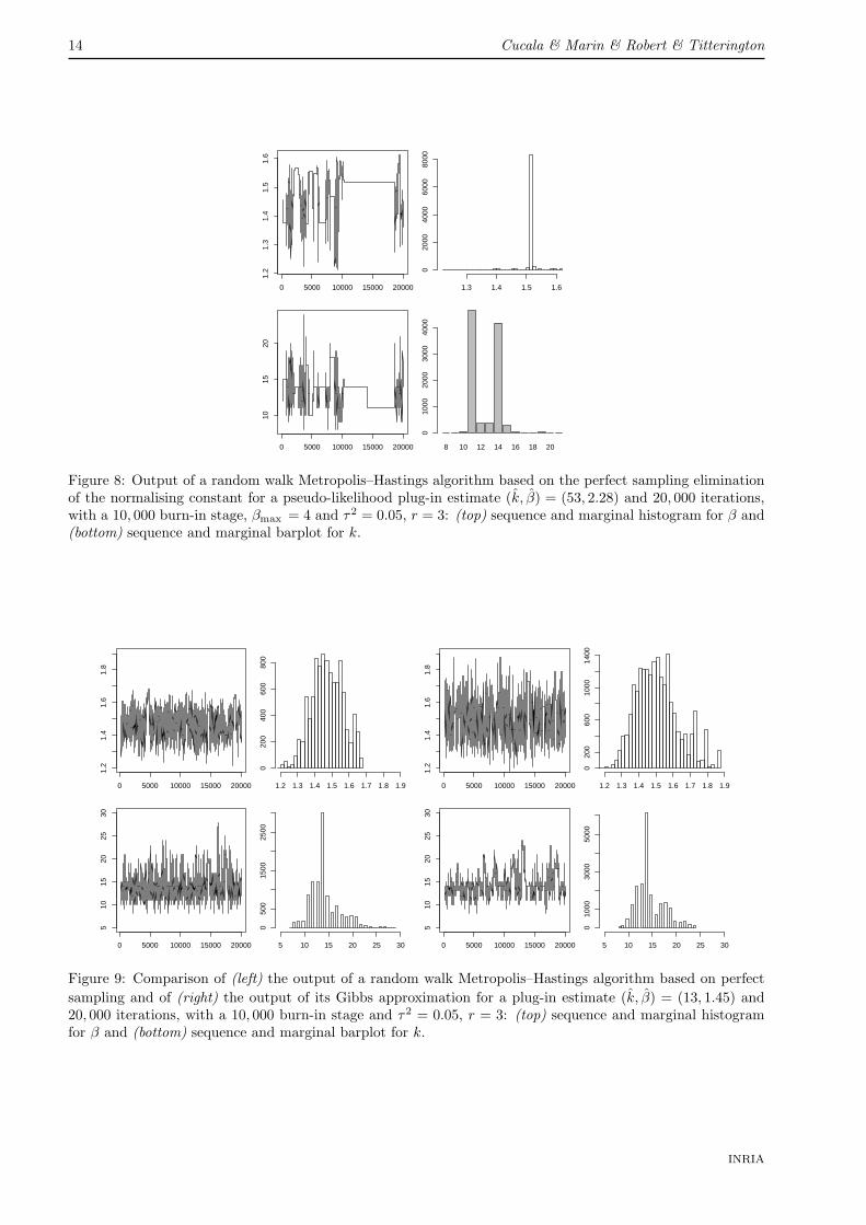
As shown on Figure 8, a poor choice for (β, k) leads to very unsatisfactory performance with the algorithm.Starting from the pseudo-likelihood estimate and using this very value for the plug-in value (β, k), we obtaina Markov chain with a very low energy and a very high rejection rate. However, use of the estimate (k, β) =(13, 1.45) resulting from this poor run does improve considerably the performance of the algorithm, as shownby Figure 9. In this setting, the predictive error rate on the test dataset is equal to 0.084.

While this elegant solution based on an auxiliary variable completely removes the issue of the normalisingconstant, it faces several computational difficulties. First, as noted above, the choice of the artificial targetg(z|β, k,y) is driving the algorithm and plug-in estimates need to be reassessed periodicaly. Second, perfectsimulation from the distribution f(z|β, k) is extremely costly and may fail if β is close to the phase-transitionboundary. Furthermore, the numerical value of this critical point is not known beforehand. Finally, theextension of the perfect sampling scheme to more than G = 2 classes has not yet been achieved.

For these different reasons, we advocate the substitution of a Gibbs sampler for the above perfect samplerin order to achieve manageable computing performance. If we replace the perfect sampling step with 500(complete) iterations of the corresponding generic Gibbs sampler on z, the computing time is linear in thenumber n of observations and the results are virtually the same. One has to remember that the simulation ofz is of second-order with respect to the original problem of simulating the posterior distribution of (β, k), since

RR n° 6173


0 5000 10000 15000 20000

1.2

1.3

1.4

1.5

1.6

Fre

quen

cy

1.3 1.4 1.5 1.6

020

0040

0060

0080

00

0 5000 10000 15000 20000

1015

20

8 10 12 14 16 18 20

010

0020

0030

0040

00

Figure 8: Output of a random walk Metropolis–Hastings algorithm based on the perfect sampling eliminationof the normalising constant for a pseudo-likelihood plug-in estimate (k, β) = (53, 2.28) and 20, 000 iterations,with a 10, 000 burn-in stage, βmax = 4 and τ2 = 0.05, r = 3: (top) sequence and marginal histogram for β and(bottom) sequence and marginal barplot for k.

0 5000 10000 15000 20000

1.2

1.4

1.6

1.8

Fre

quen

cy

1.2 1.3 1.4 1.5 1.6 1.7 1.8 1.9

020

040

060

080

0

0 5000 10000 15000 20000

510

1520

2530

Fre

quen

cy

5 10 15 20 25 30

050

015

0025

00

0 5000 10000 15000 20000

1.2

1.4

1.6

1.8

Fre

quen

cy

1.2 1.3 1.4 1.5 1.6 1.7 1.8 1.9

020

060

010

0014

00

0 5000 10000 15000 20000

510

1520

2530

Fre

quen

cy

5 10 15 20 25 30

010

0030

0050

00

Figure 9: Comparison of (left) the output of a random walk Metropolis–Hastings algorithm based on perfectsampling and of (right) the output of its Gibbs approximation for a plug-in estimate (k, β) = (13, 1.45) and20, 000 iterations, with a 10, 000 burn-in stage and τ2 = 0.05, r = 3: (top) sequence and marginal histogramfor β and (bottom) sequence and marginal barplot for k.

INRIA


0.0 0.5 1.0 1.5 2.0

01

23

4

0 1 2 3 4

01

23

45

0 1 2 3 4

02

46

0 1 2 3 4

01

23

4

Figure 10: Comparison of the approximations to the posterior distribution of β based on the pseudo (red),the path (green) and the perfect (yellow) schemes for Ripley’s benchmark and k = 1, 10, 70, 125, for 20, 000iterations and 10, 000 burn-in.

z is an auxiliary variable introduced to overcome the computation of the normalising constant. Therefore,the additional uncertainty induced by the use of the Gibbs sampler is far from severe. Figure 9 compares theGibbs solution with the perfect sampling implementation and it shows how little loss is incurred by the use ofthe less expensive Gibbs sampler, while the gain in computing time is enormous. For 50, 000 iterations, thetime required to run the Gibbs sampler is approximately 20 minutes, compared with more than a week for thecorresponding perfect sampler (under the same C environment on the same machine).

3.5 Evaluation of the pseudo-likelihood approximation

Given that the above alternatives can all be implemented for small values of n, it is of direct interest to comparethem in order to evaluate the effect of the pseudo-likelihood approximation. As demonstrated in the previoussection, using Ripley’s benchmark with a training set of 250 points, we are indeed able to run a perfect samplerover the range of possible β’s, and this implementation gives a sampler in which the only approximation is dueto running an MCMC sampler (a feature common to all three versions).

Histograms, for the same dataset, of simulated β’s, conditional or unconditional, on k show gross misrep-resentation of the samples produced by the pseudo-likelihood approximation; see Figures 10 and 11. (Thecomparison for a fixed value of k was obtained directly by setting k to a fixed value in all three approaches andrunning the corresponding MCMC algorithms.) It could of course be argued that the defect lies with the pathsampling evaluation of the constant, but this approach strongly coincides with the perfect sampling imple-mentation, as showed on both figures. There is thus a fundamental discrepancy in using the pseudo-likelihoodapproximation; in other words, the pseudo-likelihood approximation defines a clearly different posterior distri-bution on (β, k).

As exhibited on Figure 10, the larger k is, the worse is this discrepancy, whereas Figure 11 shows thatboth β and k are significantly overestimated by the pseudo-likelihood approximation. (It is quite natural tofind such a correlation between β and k when we realise that the likelihood depends mainly on β/k.) We canalso note that the correspondence between path and perfect approximations is not absolute in the case of k, adifference that may be attributed to slower convergence in one or both samplers.

In order to assess the comparative predictive properties of both approaches, we also provide a comparisonof the class probabilities P(y = 1|x,y,X) estimated at each point of the test sample. As shown by Figure 12,the predictions are quite different for values in the middle of the range, with no clear bias direction in using

RR n° 6173


0 1 2 3 4

01

23

40

500

1500

2500

3500

050

015

0025

0035

000

500

1500

2500

3500

Figure 11: Comparison of posterior distributions of β (top) and k (bottom) as represented in Figure 4 for thepseudo-likelihood approximation, in Figure 7 for the path sampling approximation and in Figure 9 for theperfect sampling approximation.

++

+

+

++++

+

++++

+

+

+ +

+

++++

+

+

+

+

+++++++

++++++

+

+ +++++

+

++++

+++

++

+

++

++++++++

++

+

++

++

+

+

+++++++

+++

+

++

+

++++

+

++

++

+ +++

+

+++

+

+++

+

+

+

++

+

+

+

+++

+

+

+

+++ ++++

+

+++

+

++++++++++

+

+

+

+

+

+

+

+

+++++++

+

+

+

+

+

+++++++++++

++

+

+++

++

+++

+

++

+

+++

+++++++++++

+

+

+

+

+

+

+++++

+++++++

+++++

+

++++

+

+

+++++

++

+

+

+

++++

+

++ +

+

+

++

++++

+

+

+

++

++

+

+

+

+

+

++

+

+ +++

+++++ +

+

+

+ ++++ +

+

+

+++

+

++

++

+

+

++

+

+++

+

+++

+

+

+++

+++ +

+

+

+ ++++

+

++ +

+

+

+

+

++

+

+++

+

++

+

+++

+

++

+

++ + ++

+

++

+++

+

+

+

+

+

+

+

+

+

+++ +

+

+++

++

+

+

+

+

++

++

+

++

++++

+

+

+

++

+

++

+ +

+

+ +

+

++

+

+

+++

+++

+++

+

+

+

++

+

+

++

++

+

+

++++ ++

++

++

+++

+

+

+

++

+

+

+

++

+

++

+

+

++

+

+

+

+

+

+

+

+

++

+

+

+

+++

+

++++

+

+

+++

+

+

++

+

+

+

+

+

+

+

+

+

+

+

++

+

+

+

++

++

+

+

++

++

+

+

++++

+

+

+

+

+

+

+

+

++++++

+

+

+

++

++

+

+++

++

+ +

+

+

++

+++

+

+

++++

+

++

+

+++

+

+++++

++ +

+

+

+++

++++++

+

+

+

+++

+

+

+

+

++

+

++

+++

++

+++

+

+

++

++

+

+

+

+

++

+

++

+++

+

+

+

+

+

+

+

+

+++

+++

+

++ +

+++++

+

+++

+++

+

+

++

+

+++

+

+

+++

+

+

++++

+

+

+

++++++++

++++++

+

+

+

+++++

+

+++

+

+

+

+

+

+

++

+

+

+

+

+

+

+

++

+++

+

++

+

+

+

+

+

+

+

+

+

+

+

+

+

+

+

+

++

+++

+++++

++

+

+

+

+

+

+

+

+

+

+

+

++

++

+

+

+

+

+

+

+

++

++

+

+

+

+

+

+

+

+

+

+

++

+++++

+

+

+

+

+

+

+

++

+

+

+

++++

+

+

+

+

+

+

+

+

+

+

+

+

++

+

+

+

+

+

+

++++

+

+

+

+

+

+

+

+++

+

+

+

+

+

+

+

+

++

+

+

+

++

+

+

+

+

+

+

+

+

+

+

+

+

+

+

+

+

+

+

+

+

+ +

+

+

+++

+

++

+

+

+

+

+

+

+

+

+

+

+

+

++

+

+

++

+++

+

+

++++

+

+

+

+++

++

++

++

+

++

++

+

+

+

+

+

+

++

+

+

+

+

+

+

+

+

+

+

+

+

++

+++

+

++

++

+

+++++++

+

+

+

+ +

0.0 0.2 0.4 0.6 0.8 1.0

0.0

0.2

0.4

0.6

0.8

1.0

Pseudo−likelihood approximation

Aux

illia

ry v

aria

ble

sche

me

with

Per

fect

sam

plin

g im

plem

enta

tion

Figure 12: Comparison of the class probabilities P(y = 1|x,y,X) estimated at each point of the testing sample.

pseudo-likelihood as an approximation. Note that the discrepancy may be substantial and may result in alarge number of different classifications.

INRIA


0 10000 30000 50000

0.8

0.9

1.0

1.1

1.2

1.3

1.4

Fre

quen

cy

0.8 0.9 1.0 1.1 1.2 1.3 1.4

020

040

060

080

010

00

0 10000 30000 50000

010

2030

4050

6070

0 28 35 42 49 56 63 70

050

010

0015

00

Figure 13: Pima Indian diabetes study based on 50, 000 iterations of the Gibbs-Møller sampling scheme withτ2 = 0.05, r = 3, βmax = 4, and K = 68.

4 Illustration on real datasets

In this Section, we illustrate the behaviour of the proposed methodology on some benchmark datasets.We first describe the calibration of the algorithm used on each dataset. As starting value for the Gibbs

approximation in the Møller scheme, we use the maximum pseudo-likelihood estimate. The Gibbs sampler isiterated 500 times as an approximation to the perfect sampling step. After 10,000 iterations, we modify theplug-in estimate using the current average and then we run 50,000 more iterations of the algorithm.

The first dataset is borrowed from the MASS library of R. It consists in the records of 532 Pima Indianwomen who were tested by the U.S. National Institute of Diabetes and Digestive and Kidney Diseases fordiabetes. Seven quantitative covariates were recorded, along with the presence or absence of diabetes. Thedata are split at random into a training set of 200 women, including 68 diagnosed with diabetes, and a testset of the remaining 332 women, including 109 diagnosed with diabetes. The performance for various valuesof k on the test dataset is given in Table 2. If we use a standard leave-one-out cross-validation for selectingk (using only the training dataset), then there are 10 consecutive values of k leading to the same error rate,namely the range 57–66.

k Misclassificationerror rate

1 0.3163 0.22915 0.22631 0.21157 0.20566 0.208

Table 2: Performance of k-nearest-neighbour methods on the Pima Indian test dataset.

The results are provided in Figure 13. Note that the simulated values of k tend to avoid the region foundby the cross-validation procedure. One possible reason for this discrepancy is that, as noted in Section 2.2,the likelihood for our joint model is not directly equivalent to the k-nearest-neighbour objective function, sincemutual neighbours are weighted twice as heavily as single neighbours in this likelihood. Over the final 20, 000iterations, the prediction error is 0.209, quite in line with the k-nearest-neighbour solution in Table 2.

RR n° 6173


To illustrate the ability of our method to consider more than two classes, we also used the benchmarkdataset forensic glass fragments, studied in Ripley (1994). This dataset involves nine covariates and six classessome of which are rather rare. Following the recommendation made in Ripley (1994), we coalesced some classesto reduce the number of classes to four. We then randomly partitioned the dataset to obtain 89 individualsin the training dataset and 96 in the testing dataset. Leave-one-out cross-validation leads us to choose thevalue k = 17. The error rate of the 17-nearest-neighbour procedure on the test dataset is 0.35, whereas, usingour procedure, we obtain an error rate of 0.29. The substantial gain from using our approach can be partiallyexplained by the fact that the value of k chosen by the cross-validation procedure is much larger than thoseexplored by our MCMC sampler.

5 Conclusions

While the probabilistic background to a Bayesian analysis of k-nearest-neighbour methods was initiated byHolmes and Adams (2003), the present paper straightens the connection between the original technique and atrue probabilistic model by defining a coherent probabilistic model on the training dataset. This new model(3) then provides a sound setting for Bayesian inference and for evaluating not just the most likely allocationsfor the test dataset but also the uncertainty that goes with them. The advantages of using a probabilisticenvironment are clearly demonstrated: it is only within this setting that tools like predictive maps as in Figure3 can be constructed. This obviously is a tremendous bonus for the experimenter, since boundaries betweenmost likely classes can thus be estimated and regions can be established in which allocation to a specific class orto any class is uncertain. In addition, the probabilistic framework allows for a natural and integrated analysisof the number of neighbours involved in the class allocation, in a standard model-choice perspective. Thisperspective can be extended to the choice of the most significant components of the covariate x, even thoughthis possibility is not explored in the current paper.

The present paper also addresses the computational difficulties related to this approach, namely the well-known issue of the intractable normalising constant. While this has been thoroughly discussed in the literature,our comparison of three independent approximations leads to the strong conclusion that the pseudo-likelihoodapproximation is not to be trusted for training sets of moderate size. Furthermore, while the path samplingand perfect sampling approximations are useful in establishing this conclusion, they cannot be advocated at theoperational level, but we also demonstrate that a Gibbs sampling alternative to the perfect sampling schemeof Møller et al. (2006) is both operational and practical.

Acknowledgements

The authors are grateful to Gilles Celeux for his numerous and insightful comments on the different perspectivesoffered by this probabilistic reassessment, as well as to the Associate Editor and to both referees for theirconstructive comments. Both JMM and CPR are also grateful to the Department of Statistics of the Universityof Glasgow for its warm welcome during various visits related to this work. This work was supported in part bythe IST Programme of the European Community, under the PASCAL Network of Excellence, ST-2002-506778.

References

Berthelsen, K. and Møller, J. (2003). Likelihood and non-parametric Bayesian MCMC inference for spatialpoint processes based on perfect simulation and path sampling. Scandinavian J. Statist., 30:549–564.

Besag, J. (1974). Spatial interaction and the statistical analysis of lattice systems (with discussion). J. Roy.Statist. Soc. Ser. B, 36:192–236.

Besag, J. and Kooperberg, C. (1995). On conditional and intrinsic autoregressions. Biometrika, 82(4):733–746.

Besag, J., York, J., and Mollie, A. (1991). Bayesian image restoration, with two applications in spatial statistics.Ann. Inst. Statist. Math., 43(1):1–59. With discussion and a reply by Besag.

Buhlmann, P. (2004). Bagging, boosting and ensemble methods. In Handbook of Computational Statistics,pages 877–907. Springer, Berlin.

Buhlmann, P. and Yu, B. (2002). Analyzing bagging. Ann. Statist., 30(4):927–961.

INRIA


Buhlmann, P. and Yu, B. (2003). Boosting with the L2 loss: regression and classification. J. Amer. Statist.Assoc., 98(462):324–339.

Buttrey, S. (1998). Nearest-neighbor classification with categorical variables. Comp. Stat. Data Analysis,28:157–169.

Chen, M., Shao, Q., and Ibrahim, J. (2000). Monte Carlo Methods in Bayesian Computation. Springer, NewYork.

Cressie, N. A. C. (1993). Statistics for Spatial Data. Wiley Series in Probability and Mathematical Statistics:Applied Probability and Statistics. John Wiley & Sons Inc., New York.

Devroye, L., Gyorfi, L., and Lugosi, G. (1996). A Probabilistic Theory of Pattern Recognition, volume 31 ofApplications of Mathematics (New York). Springer-Verlag, New York.

Freund, Y. and Schapire, R. E. (1997). A decision-theoretic generalization of on-line learning and an applicationto boosting. J. Comput. System Sci., 55(1, part 2):119–139. Second Annual European Conference onComputational Learning Theory (EuroCOLT ’95) (Barcelona, 1995).

Friel, N., Pettitt, A., Reeves, R., and Wit, E. (2005). Bayesian inference in hidden markov random fields forbinary data defined on large lattices. Technical report, Department of Statistics, University of Glasgow.

Friel, N. and Pettitt, A. N. (2004). Likelihood estimation and inference for the autologistic model. J. Comput.Graph. Statist., 13(1):232–246.

Gelman, A. and Meng, X.-L. (1998). Simulating normalizing constants: from importance sampling to bridgesampling to path sampling. Statist. Sci., 13(2):163–185.

Haggstrom, O. (2002). Finite Markov Chains and Algorithmic Applications, volume 52 of Student Texts.London Mathematical Society.

Hastie, T., Tibshirani, R., and Friedman, J. (2001). The Elements of Statistical Learning. Springer Series inStatistics. Springer-Verlag, New York.

Heikkinen, J. and Hogmander, H. (1994). Fully Bayesian approach to image restoration with an application inbiogeography. J. R. Stat. Soc. Ser. C, 43(4):569–582.

Hoeting, J. A., Madigan, D., Raftery, A., and Volinsky, C. (1999). Bayesian model averaging: A tutorial (withdiscussion). Statistical Science, 14(4):382–417.

Holmes, C. C. and Adams, N. M. (2002). A probabilistic nearest neighbour method for statistical patternrecognition. J. R. Stat. Soc. Ser. B Stat. Methodol., 64(2):295–306.

Holmes, C. C. and Adams, N. M. (2003). Likelihood inference in nearest-neighbour classification models.Biometrika, 90(1):99–112.

Kendall, W. and Møller, J. (2000). Perfect simulation using dominating processes on ordered spaces, withapplication to locally stable point processes. Advances in Applied Probability, 32:844–865.

Manocha, J. and Girolami, M. (2007). An empirical analysis of the probabilistic K-nearest neighbour classifier.Pattern Recognition Letters, pages 1818–1824.

McLachlan, G. J. (1992). Discriminant Analysis and Statistical Pattern Recognition. Wiley Series in Probabilityand Mathematical Statistics: Applied Probability and Statistics. John Wiley & Sons Inc., New York.

Møller, J. (2003). Spatial Statistics and Computational Methods, volume 173 of Lecture Notes in Statistics.Springer-Verlag, New York.

Møller, J., Pettitt, A., Reeves, R., and Berthelsen, K. (2006). An efficient Markov chain Monte Carlo methodfor distributions with intractable normalising constants. Biometrika, 93:451–458.

Møller, J. and Waagepetersen, R. (2003). Statistical Inference and Simulation for Spatial Point Processes.Chapman and Hall/CRC, Boca Raton, FL.

RR n° 6173


Ogata, Y. (1989). A Monte Carlo method for high-dimensional integration. Numer. Math., 55(2):137–157.

Propp, J. and Wilson, D. (1998). Coupling from the past: a user’s guide. In Microsurveys in discrete probability(Princeton, NJ, 1997), volume 41 of DIMACS Ser. Discrete Math. Theoret. Comput. Sci., pages 181–192.Amer. Math. Soc., Providence, RI.

Ripley, B. D. (1994). Neural networks and related methods for classification (with discussion). J. Roy. Statist.Soc. Ser. B, 56(3):409–456.

Ripley, B. D. (1996). Pattern Recognition and Neural Networks. Cambridge University Press, Cambridge.

Robert, C. (2001). The Bayesian Choice. Springer Texts in Statistics. Springer-Verlag, New York, secondedition.

Robert, C. P. and Casella, G. (2004). Monte Carlo Statistical Methods. Springer Texts in Statistics. Springer-Verlag, New York, second edition.

Zhang, T. and Yu, B. (2005). Boosting with early stopping: convergence and consistency. Ann. Statist.,33(4):1538–1579.

INRIA

Unité de recherche INRIA FutursParc Club Orsay Université - ZAC des Vignes

4, rue Jacques Monod - 91893 ORSAY Cedex (France)

Unité de recherche INRIA Lorraine : LORIA, Technopôle de Nancy-Brabois - Campus scientifique615, rue du Jardin Botanique - BP 101 - 54602 Villers-lès-Nancy Cedex (France)

Unité de recherche INRIA Rennes : IRISA, Campus universitaire de Beaulieu - 35042 Rennes Cedex (France)Unité de recherche INRIA Rhône-Alpes : 655, avenue de l’Europe - 38334 Montbonnot Saint-Ismier (France)

Unité de recherche INRIA Rocquencourt : Domaine de Voluceau - Rocquencourt - BP 105 - 78153 Le Chesnay Cedex (France)Unité de recherche INRIA Sophia Antipolis : 2004, route des Lucioles - BP 93 - 06902 Sophia Antipolis Cedex (France)

ÉditeurINRIA - Domaine de Voluceau - Rocquencourt, BP 105 - 78153 Le Chesnay Cedex (France)

http://www.inria.fr

ISSN 0249-6399

A Bayesian reassessment of nearest-neighbour classification

Documents

Transcript of A Bayesian reassessment of nearest-neighbour classification