Automatic Choice of the Number of Nearest Neighbors in ...

Automatic Choice of the Number of Nearest

Neighbors in Locally Linear Embedding

Juliana Valencia-Aguirre, Andres Alvarez-Mesa, Genaro Daza-Santacoloma,and German Castellanos-Domınguez

Control and Digital Signal Processing Group, Universidad Nacional de Colombia,Manizales, Colombia

{jvalenciaag,amalvarezme,gdazas,cgcastellanosd}@unal.edu.co

Abstract. Locally linear embedding (LLE) is a method for nonlineardimensionality reduction, which calculates a low dimensional embeddingwith the property that nearby points in the high dimensional space re-main nearby and similarly co-located with respect to one another in thelow dimensional space [1]. LLE algorithm needs to set up a free param-eter, the number of nearest neighbors k. This parameter has a stronginfluence in the transformation. In this paper is proposed a cost func-tion that quantifies the quality of the embedding results and computesan appropriate k. Quality measure is tested on artificial and real-worlddata sets, which allow us to visually confirm whether the embedding wascorrectly calculated.

1 Introduction

In many pattern recognition problems the characterization stage generates a bigamount of data. There are several important reasons for reducing the featurespace dimensionality, such as, improve the classification performance, diminishirrelevant or redundancy information, find out underlying data structures, obtaina graphical data representation for visual analysis, etc [2]. Several techniques fordimensionality reduction have been developed, traditionally these techniques arelinear [3] and they can not correctly discover underlying structures of data lie onnonlinear manifolds. In order to solve this trouble a nonlinear mapping methodcalled locally linear embedding (LLE) was proposed in [4,5].

This method requires to manually set up three free parameters, the dimen-sionality of embedding space m, the regularization parameter α, and the numberof nearest neighbors k for local analysis [6]. There are two previous approachesfor choosing k. Kouropteva et. al [7] presented a hierarchical method for auto-matic selection of an optimal parameter value based on the minimization of theresidual variance. Nonetheless, the residual variance can not quantify the localgeometric structure of data. Besides, Goldberg and Ritov [8] display a novelmeasure based on Procrustes rotation that enables quantitative comparison ofthe output of manifold-based embedding algorithms, the measure also serves as anatural tool for choosing dimension-reduction parameters. The local procrustes

E. Bayro-Corrochano and J.-O. Eklundh (Eds.): CIARP 2009, LNCS 5856, pp. 77–84, 2009.c© Springer-Verlag Berlin Heidelberg 2009

78 J. Valencia-Aguirre et al.

measure preserves local geometric structure but does not consider the globalbehavior of the manifold.

In this paper is proposed an automatic method for choosing the number ofnearest neighbors, which is done by means of computing a cost function thatquantifies the quality of embedding space. This function takes into account localand global geometry preservation. Proposed approach is experimentally verifiedon 2 artificial data sets and 1 real-world data set. Artificial data sets allow tovisually confirm whether the embedding was correctly calculated, and real-worlddata set was used for visualization of multidimensional samples.

2 Locally Linear Embedding

Let X the input data p×n matrix, where the sample vectors xi ∈ �p, i = 1, . . . , nare had. Data live on or close to a non-linear manifold and that is well-sampled.Besides, each point and its neighbors lie on a locally linear patch. LLE algorithmhas 3 steps. First, search the k nearest neighbors per point, as measured byEuclidean distance. If k is set too small, the mapping will not reflect any globalproperties; if it is too high, the mapping will lose its nonlinear character andbehave like traditional PCA [6]. Second, each point is represented as a weightedlinear combination of its neighbors [9], that is, we calculate weights W thatminimize reconstruction error

ε (W) =n∑

i=1

‖xi −n∑

j=1

wijxj‖2, (1)

subject to an sparseness constraint, wij = 0 if xj is not k−neighbor of xi, andan invariance constraint

∑nj=1 wij = 1. For a particular data point x ∈ �p and

its k nearest neighbors ηηη. Let G the Gram k× k matrix, where its elements areGjl =

⟨(x− ηηηj

), (x− ηηηl)

⟩, j = 1, . . . , k; l = 1, . . . , k. Then rewriting (1)

ε = w�Gw s.t.∑n

j=1wj = 1. (2)

The solution of (2) is obtained by solving an eigenvalue problem. EmployingLagrange theorem w = (1/2)λG−11, where λ = 2

/(1�G−11

). When Gram

matrix G is singular (or close), the result of least squares problem for finding wdoes not have unique solution. So, it is necessary to regularize G before findingw. In [1,5] is proposed to calculate the regularization of G as Gjl ← Gjl + αwhere α = δjl

(Δ2

/k)tr (G), being δjl = 1 if j = l and 0 in other case, Δ2 � 1.

However, Δ must be empirically tuned, in [1] is advised to employ Δ = 0.1.In third step low dimensional embedding is calculated. Using W, the low

dimensional output Y is found by minimizing (3)

Φ (Y) =n∑

i=1

‖yi −n∑

j=1

wijyj‖2, (3)

Automatic Choice of the Number of Nearest Neighbors in LLE 79

subject to∑n

i=1 yi = 0 and∑n

i=1 yiy�i /n = Im×m, where Y is the embedding

data n×m matrix (being m ≤ p), and yi ∈ �m is the output sample vector.Let M =

(In×n −W�)

(In×n −W), and rewriting (3) to find Y,

Φ (Y) = tr(Y�MY

)s.t.

{11×nY = 01×n1nY�Y = Im×m

(4)

it is possible to calculate m + 1 eigenvectors of M, which are associated tom + 1 smallest eigenvalues. First eigenvector is the unit vector with all equalcomponents, which is discarded. The remaining m eigenvectors constitute the membedding coordinates found by LLE.

3 Measure of Embedding Quality

When dimensionality reduction technique is computed is necessary to establisha criteria for knowing if its results are adequate. In LLE is searched a transfor-mation that preserves the local data geometry and global manifold properties.

The quality of an output embedding could be judged based on a comparison tothe structure of the original manifold. However, in the general case, the manifoldstructure is not given, and it is difficult to estimate accurately. As such idealmeasures of quality cannot be used in the general case, an alternate quantitativemeasure is required [8].

In [7], the residual variance is employed as a quantitative measure of theembedding results. It is defined as

σ2R(DX, DY) = 1− ρ2

DXDY, (5)

where ρ2 is the standard linear correlation coefficient, taken over all entries ofDX and DY; DX and DY are the matrices for Euclidean distances in X and Y,respectively. DY depends on the number of neighbors selected k. According to[7], the lowest residual variance corresponds to the best high-dimensional datarepresentation in the embedded space. Hence, the number of neighbors can becomputes as

kσ2R

= argmink

(σ2R(DX, DY)). (6)

On the other hand, in [8] is proposed to compare a neighborhood on the mani-fold and its embedding using the Procrustes statistic as a measure for qualifyingthe transformation. This measures the distance between two configurations ofpoints and is defined as P (X,Y) =

∑ni=1 ‖xi −Ayi − b‖2, being A�A = I

and b ∈ �m. The rotation matrix A can be computed from Z = X�HY, whereH = I− 1

k11�, 1 is a n × 1 column vector, and H is the centering matrix. LetULV� be the singular-value decomposition of Z, then A = UV�, the trans-lation vector b = x −Ay, where x and y are the sample means of X and Y,respectively. Let ‖·‖F the Frobenius norm, so P (X,Y) = ‖H(X−YA�)‖2F .

In order to define how well an embedding preserves the local neighborhoodsusing the Procrustes statistic PL(Xi,Yi) of each neighborhood-embedding pair


(Xi,Yi). PL (Xi,Yi) estimates the relation between the entire input neighbor-hood and its embedding as one entity, instead of comparing angles and distanceswithin the neighborhood with those within its embedding. A global embeddingthat preserves the local structure can be found by minimizing the sum of theProcrustes statistics of all neighborhood-embedding pairs [8], taking into ac-count an scaling normalization, which solves the problem of increased weightingfor larger neighborhoods, so

RN (X,Y) =1n

n∑

i=1

PL(Xi,Yi)/ ‖HLXi‖2F , (7)

where HL = I− 1k11�; 1 is a k × 1 vector. Therefore, the number of nearest

neighbors can be calculated as

kRN = arg mink

(RN (X,Y)). (8)

In this work, we propose an alternative measure for quantifying the embeddingquality. This measure attempts to preserve the local geometry and the neigh-borhood co-location, identifying possible overlaps on the low dimensional space.And it is defined as

CI (X,Y) =

12n

n∑

i=1

⎧⎨

⎩1k

k∑

j=1

(D(xi,ηηηj) −D(yi,φφφj)

)2

+1kn

kn∑

j=1

(D(xi,θθθj) −D(yi,γγγj)

)2

⎫⎬

⎭,(9)

where D is an standardized Euclidean distance to obtain a maximum value equalto one. For example D(xi,ηηηj) is the distance calculated between the observationxi and each one of its k neighbors on the input space.

Once the embedding, for each point yi ∈ �m a set βββ of k nearest neighborsis calculated, and the projection φφφ of ηηη is found. The neighbors computed in βββthat are not neighbors in ηηη conform a new set γγγ, that is γγγ = βββ − (βββ ∩φφφ). Thesize of γγγ is kn. Besides, the projections of the elements of γγγ in X conform theset θθθ of kn neighbors. In an ideal embedding CI (·) = 0.

The first term in (9) quantifies the local geometry preservation. The k nearestneighbors of xi chosen on the high dimensional space X are compared againsttheir representations in the embedded space Y. The second term computes theerror produced by possible overlaps in the embedded results, which frequentlyoccurs when the number of neighbors is strongly increased, and global propertiesof the manifold are lost. The number of nearest neighbors can be found as

kCI = arg mink

(CI(X,Y)). (10)

4 Experimental Background

4.1 Tests on Artificial Data Sets

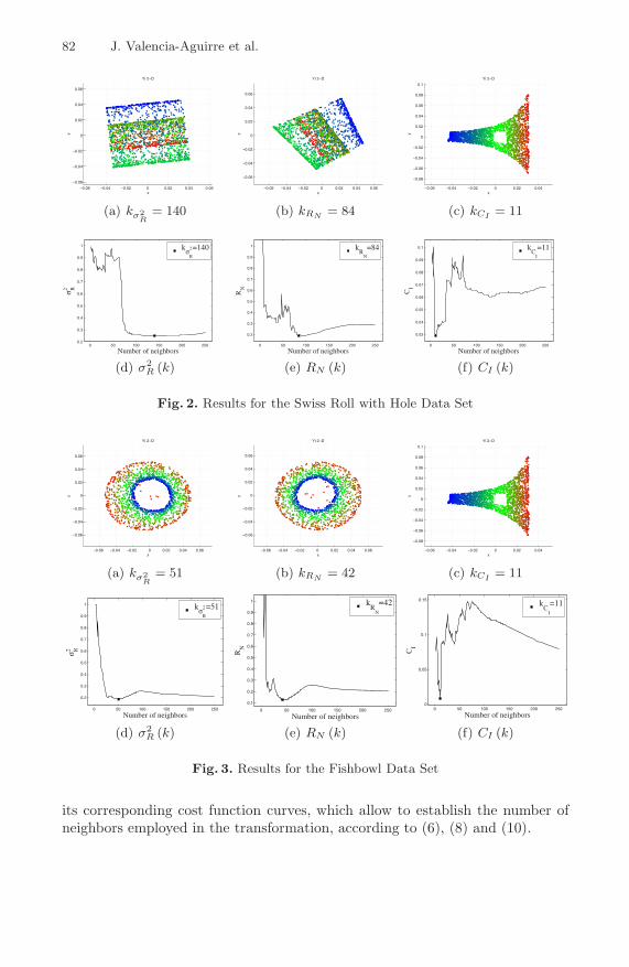
Two different manifold are tested, which allow to visually confirm whether theembedding was correctly calculated. The Swiss Roll with Hole data set with


−15 −10 −5 0 5 10 150

1020

−15

−10

−5

0

5

10

z

Xi 3−D

x

y

(a) Swiss Roll with Hole

−1.5 −1 −0.5 0 0.5 1 1.5−1

01

−1

−0.5

0

0.5

1

z

Xi 3−D

x

y

(b) Fishbowl

Fig. 1. Artificial Data Sets

2000 samples (Fig. 1(a)) and the Fishbowl data set with uniform distribution inembedding space and 1500 samples (Fig. 1(b)).

In order to quantify the embedding quality and find the number of nearestneighbors needed for a faithful embedding, LLE is computed by varying k in thesubset k ∈ {3, 4, 5, . . . , 250}, fitting the dimensionality of the embedded space tom = 2. The embedding quality is computed according to (5), (7) and (9). Thenumber of nearest neighbors is found by means of (6), (8) and (10).

In Figures 2(a), 2(b), and 2(c) are presented the embedding results for theSwiss Roll with Hole data set using an specific number of neighbors in accordancewith each one of the criteria above pointed out. Similarly, in Figures 3(a), 3(b),and 3(c) the embedding results for the Fishbowl data set are displayed. For theseartificial data sets only our approach (10) finds appropriate embedding resultspreserving local and global structure. In the case of the Swiss Roll with Hole, thecriteria (6) and (8) produce overlapped embeddings. Besides, in Fishbowl, theunfolding results obtained by means of (6) and (8) are wrong, those are similarto PCA and then local structure is lost.

On the other hand, Figures 2(d), 2(e), 2(f), and 3(d), 3(e), 3(f), show curvesof the cost function value versus the number of neighbors. The full fill square onthe curves is the global minimum of the function and corresponds to the numberof nearest neighbors chosen for the embedding.

4.2 Tests on Real-World Data Sets

We use Maneki Neko pictures, which is in the Columbia Object Image Library(COIL-100) [10]. There are 72 RGB-color images for this object in PNG format.Pictures are taken while the object is rotated 360 degrees in intervals of 5 degrees.The image size is 128× 128. In Fig. 4 are shown some examples. We transformthese color images to gray scale, next the images were subsampled to 64 × 64pixels. Then, we have input space of dimension p = 8192 and n = 72.

In order to quantify the embedding quality and find the number of neighborsneeded for a faithful embedding, LLE is computed by varying k in the subsetk ∈ {3, 4, 5, . . . , 36}, fitting the dimensionality of the embedded space to m = 2.In Fig. 5 are shown the embedding results for the Maneki Neko data set and


−0.06 −0.04 −0.02 0 0.02 0.04 0.06

−0.06

−0.04

−0.02

0

0.02

0.04

0.06

Yi 2−D

x

y

(a) kσ2R

= 140

−0.06 −0.04 −0.02 0 0.02 0.04 0.06

−0.06

−0.04

−0.02

0

0.02

0.04

0.06

Yi 2−D

x

y

(b) kRN = 84

−0.06 −0.04 −0.02 0 0.02 0.04

−0.08

−0.06

−0.04

−0.02

0

0.02

0.04

0.06

0.08

0.1

Yi 2−D

x

y

(c) kCI = 11

0 50 100 150 200 2500.2

0.3

0.4

0.5

0.6

0.7

0.8

0.9

1

Number of neighbors

σ2 R

kσ2

R

=140

(d) σ2R (k)

0 50 100 150 200 250

0.2

0.3

0.4

0.5

0.6

0.7

0.8

0.9

1

Number of neighbors

RN

kR

N

=84

(e) RN (k)

0 50 100 150 200 250

0.03

0.04

0.05

0.06

0.07

0.08

0.09

0.1

Number of neighbors

CI

kC

I

=11

(f) CI (k)

Fig. 2. Results for the Swiss Roll with Hole Data Set

−0.06 −0.04 −0.02 0 0.02 0.04 0.06

−0.06

−0.04

−0.02

0

0.02

0.04

0.06

Yi 2−D

x

y

(a) kσ2R

= 51

−0.06 −0.04 −0.02 0 0.02 0.04 0.06

−0.06

−0.04

−0.02

0

0.02

0.04

0.06

Yi 2−D

x

y

(b) kRN = 42

−0.06 −0.04 −0.02 0 0.02 0.04

−0.08

−0.06

−0.04

−0.02

0

0.02

0.04

0.06

0.08

0.1

Yi 2−D

x

y

(c) kCI = 11

0 50 100 150 200 250

0.2

0.3

0.4

0.5

0.6

0.7

0.8

0.9

1

Number of neighbors

σ2 R

kσ2

R

=51

(d) σ2R (k)

0 50 100 150 200 250

0.1

0.2

0.3

0.4

0.5

0.6

0.7

0.8

0.9

1

Number of neighbors

RN

kR

N

=42

(e) RN (k)

0 50 100 150 200 2500

0.05

0.1

0.15

Number of neighbors

CI

kC

I

=11

(f) CI (k)

Fig. 3. Results for the Fishbowl Data Set

its corresponding cost function curves, which allow to establish the number ofneighbors employed in the transformation, according to (6), (8) and (10).


(a) 0◦ (b) 45◦ (c) 90◦

Fig. 4. Examples from Maneki Neko Data Set

−0.2 −0.1 0 0.1 0.2−0.3

−0.2

−0.1

0

0.1

0.2

Yi 2−D

x

y

(a) kσ2R

= 6

−0.2 −0.1 0 0.1 0.2 0.3−0.3

−0.2

−0.1

0

0.1

0.2

0.3

Yi 2−D

x

y

(b) kRN = 25

-0.2 -0.1 0 0.1 0.2

-0.2

-0.1

0

0.1

0.2

0.3

Yi 2-D

x

y

(c) kCI = 4

5 10 15 20 25 30 35

0.3

0.35

0.4

0.45

0.5

0.55

0.6

0.65

Number of neighbors

σ2 R

kσ2

R

=6

(d) σ2R (k)

5 10 15 20 25 30 35

0.982

0.984

0.986

0.988

0.99

0.992

0.994

0.996

0.998

1

Number of neighbors

RN

kR

N

=25

(e) RN (k)

5 10 15 20 25 30 35

0.02

0.04

0.06

0.08

0.1

0.12

Number of neighbors

CI

kC

I

=4

(f) CI (k)

Fig. 5. Results of Maneki Neko Data Set

5 Discussion

From the obtained results on artificial data sets (Fig. 2(d) and 3(d)) employing thecost function (6) proposed in [7], as a global trend, it is possible to notice if the sizeof the neighborhood is augmented, the value of σ2

R is diminished. Because a trans-formation employing a large number of neighbors results in a linear transformationand the residual variance does not quantify the local geometric structure, then thismeasure can not identify a suitable number of neighbors k. Figures 2(a) and 3(a)show some examples of this situation. In this case, data in low-dimensional spaceare overlapped and the cost function (6) does not detect it. Nevertheless Fig. 5(d)does not display the trend above pointed out and allows to calculate an appropriateembedding (Fig. 5(a)). The inconsistent results obtainedby using the residual vari-ance make of it an unreliable measure. In [7] the ambiguous results are attributedto the fact that Euclidean distance becomes an unreliable indicator for proximity.

On the other hand, the measure proposed in [8] takes into account the localgeometric structure but does not consider the global behavior of the manifold.


Then, far neighborhoods can be overlapped in the low-dimensional space and thismeasure shall not detect it, which can be seen in Fig. 2(b), 3(b), and 5(b). Themeasure of embedding quality presented here (10) computes a suitable numberof neighbors for both artificial and real-world manifolds. Besides, the embeddingresults calculated using this criterion are in accordance to the expected visualunfolding (Fig 2(c), 3(c), and 5(c)). The proposed measure preserves the localgeometry of data and the global behavior of the manifold.

6 Conclusion

In this paper a new measure for quantifying the embedding quality using LLEis proposed. This measure is employed as a criterion for choosing automaticallythe number of nearest neighbors needed for the transformation. We comparethe new cost function against two methods presented in the literature. Thebest embedding results (visually confirmed) were obtained using the approachexposed, because it preserves the local geometry of data and the global behaviorof the manifold.

Acknowledgments. This research was carried out under grants provided bythe project Representacion y discriminacion de datos funcionales empleandoinmersiones localmente lineales funded by Universidad Nacional de Colombia,and a Ph. D. scholarship funded by Colciencias.

References

1. Saul, L.K., Roweis, S.T.: Think globally, fit locally: Unsupervised learning of lowdimensional manifolds. Machine Learning Research 4 (2003)

2. Carreira-Perpinan, M.A.: A review of dimension reduction techniques (1997)3. Webb, A.R.: Statistical Pattern Recognition, 2nd edn. Wiley, USA (2002)4. Roweis, S.T., Saul, L.K.: Nonlinear dimensionality reduction by locally linear em-

bedding. Science 290, 2323–2326 (2000)5. Saul, L.K., Roweis, S.T.: An introduction to locally linear embedding. AT&T Labs

and Gatsby Computational Neuroscience Unit, Tech. Rep. (2000)6. de Ridder, D., Duin, R.P.W.: Locally linear embedding for classification. Delft

University of Technology, The Netherlands, Tech. Rep. (2002)7. Kouropteva, O., Okun, O., Pietikainen, M.: Selection of the optimal parameter

value for the locally linear embedding algorithm. In: The 1st International Confer-ence on Fuzzy Systems and Knowledge Discovery (2002)

8. Goldberg, Y., Ritov, Y.: Local procrustes for manifold embedding: a measure ofembedding quality and embedding algorithms. Machine learning (2009)

9. Polito, M., Perona, P.: Grouping and dimensionality reduction by locally linearembedding. In: NIPS (2001)

10. Nene, S.A., Nayar, S.K., Murase, H.: Columbia object image library: Coil-100.Columbia University, New York, Tech. Rep. (1996)

Automatic Choice of the Number of Nearest Neighbors in ...

Documents

Transcript of Automatic Choice of the Number of Nearest Neighbors in ...