Seediscussions,stats,andauthorprofilesforthispublicationat:https://www.researchgate.net/publication/4765249

PathDependenceandLearningfromNeighbors

ArticleinGamesandEconomicBehavior·February1996

DOI:10.1006/game.1996.0032·Source:RePEc

CITATIONS

95

READS

34

2authors:

LucaAnderlini

GeorgetownUni…

56

PUBLICATIONS754CITATIONS

SEEPROFILE

AntonellaIanni

UniversityofSou…

14

PUBLICATIONS155CITATIONS

SEEPROFILE

AllcontentfollowingthispagewasuploadedbyAntonellaIannion01December2016.

Theuserhasrequestedenhancementofthedownloadedfile.

GAMES AND ECONOMIC BEHAVIOR13,141–177 (1996)ARTICLE NO. 0032

Path Dependence and Learning from Neighbors∗

Luca Anderlini†

St. John’s College, Cambridge, United Kingdom

Antonella Ianni

University College London, London, United Kingdom

Received May 20, 1993

We study the long-run properties of a class of locally interactive learning systems. Afinite set of players at fixed locations play a two-by-two symmetric normal form game withstrategic complementarities, with one of their “neighbors” selected at random. Because ofthe endogenous nature of experimentation, or “noise,” the systems we study exhibit a highdegree of path dependence. Different actions of a pure coordination game may survive inthe long-run at different locations of the system. A reinterpretation of our results shows thatthe local nature of search may be a robust reason for price dispersion in a search model,Journal of Economic LiteratureClassification Numbers: C72, D83.© 1996 Academic Press,

Inc.

∗ We are grateful to Ken Binmore, Tilman B¨orgers, Bob Evans, Drew Fudenberg, Alan Kirman,Daniel Probst, Rafael Rob, Hamid Sabourian, Karl Schlag, Peyton Young, and seminar participants atthe Second C.I.T.G. workshop on Game Theory, University College London, Cambridge University,Harvard University and the University of Pennsylvania for stimulating comments. We also thank twoanonymous referees for suggesting ways to improve both the substance and the exposition of the paper.Any remaining errors are, of course, our own responsibility. Some of the results reported here werefirst suggested by simulations carried out on a CAM-PC hardware board purchased with the supportof a SPES grant from the European Community; their financial assistance is gratefully acknowledged.The research of Luca Anderlini was partly supported by a gratefully acknowledged ESRC Grant R000232865 and by the generous hospitality of the Cowles Foundation for Research in Economics at YaleUniversity.

† E-mail:la13@econ.cam.ac.uk.

1410899-8256/96 $18.00

Copyright © 1996 by Academic Press, Inc.All rights of reproduction in any form reserved.

142 ANDERLINI AND IANNI

1. INTRODUCTION

1.1. Motivation

The notion of Nash equilibrium (and its various refinements) has come topervade the use of Game Theory asthe noncooperative solution concept. The“eductive” justification for Nash equilibrium has come under severe criticismby economic theorists in recent years (Binmore, 1987, 1988). The idea thatplayers can somehow introspectively “educe” how the game will be played, andhence respond optimally to it, places unreasonable demands on the computationalpowers of the players and may even be criticized as logically inconsistent in somecases (Anderlini, 1989; Binmore, 1987, 1988; Canning, 1992a).

As a consequence, much attention has been given recently to “evolutionary”and “learning” models of games. The main stance taken in this literature isthat players will react “adaptively” to the circumstances facing them. Becauseof their limited computational powers and/or because of information gatheringand computational costs, they will respond according to some fixed rule to theirpresent and past environment. They willlearnhow to play the game through time.A very closely related approach takes the stance that more successful behavioris more likely tosurviveinto the “next generation” of players, and hence a wayto play the game will “evolve” through time.

Both in the case of learning and in evolutionary models, an explicit dynamicalsystem is derived, and attention is focused on its long-run properties. In manycases, it has been possible to “justify” Nash equilibrium along these lines. Thispaper contributes to the literature on learning in games. We studylocally inter-activelearning systems in which players learn from the observation of theirlocalenvironment only. The learning systems we study do justify Nash equilibriumin a class of locally interactive systems. Together with convergence to a Nashequilibrium, the possible complexities of localized behavior emerge. “Distant”parts of the system may display different behavior in the long run and yet thesystem as a whole will be in equilibrium. We characterize fully the possiblelong-run positions of the system in one particular case.

The literature on learning and evolution in games has been growing veryfast in recent years. A comprehensive list of just the major contributions to thefield would take up far too much space. We simply recall the surveys of vanDamme (1987) and Friedman (1991), the work of Milgrom and Roberts (1990,1991), Fudenberg and Kreps (1990), Canning (1992b), Kandoriet al. (1993),Fudenberg and Maskin (1990), Binmore and Samuelson (1992), Selten (1991),Evans (1992), Young (1993), and Anderlini and Sabourian (1993).1

1 Games and Economic Behaviorpublished a double Special Issue on Adaptive Dynamics in 1993(Vol. 5, Nos. 3 and 4). We also refer to the papers therein for a comprehensive list of references and avariety of important contributions to this research program.

LEARNING FROM NEIGHBORS 143

1.2. Local Interaction and “Noise at the Margin”

The common theme of many recent contributions to the learning literature isnot difficult to outline. A population of players is given. Players are assumed touse “rules of thumb” or “learning rules” when they decide how to play the nextround of a sequence of games with which they are faced. A learning rule is anarbitrary, but appealing for a variety of unmodeled reasons, map from the pasthistory of play (or some subset of it) into what to do next. In many cases the inputof the learning rule is simply some statistic of how the last round was played.The central questions which have been addressed in the literature are those ofwhether the dynamical system describing the behavior of the population throughtime converges and, if so, to what configuration of play. With the importantexception of the analysis of systems in which the underlying game is inextensiveform,2 “adaptive” rules of thumb which embody some form or other of myopicoptimization have almost invariably been found to have the property that ifconvergence obtains, the limit configuration of play is a Nash equilibrium of theunderlying game.

In many cases (Kandori,et al., 1993; Young, 1993; Binmore and Samuelson,1992; Fudenberg and Maskin, 1990) the characterization of the limit configu-ration of play obtained is much more stringent than Nash equilibrium. A roughoutline of some of these equilibrium selection results is as follows. The ruleof thumb which players use is a simple myopic optimization based on the pro-portions of players which took each action in the last round or lastn roundsof play. The system considered has, by assumption, a finite number of possiblestates which represent all possible configurations of play for all the players. Ifthe learning rules which players use have finite memory it is easy to see howthe entire dynamical system can be viewed as a finite Markov chain. Supposenow that in each period players may deviate from the behavior prescribed by thelearning rule they are using because they make “mistakes” with some positive(small) probability. For simplicity’s sake imagine that mistakes may make anyplayer take any action with positive probability at any time. Then, by standardresults, the Markov chain describing the behavior of the system will display auniqueergodic distribution. This is the limit configuration of play as time goes toinfinity. The limit configuration of play is “parameterized” by the constant prob-ability of mistakes in each period. A second limit can then be characterized moreor less stringently according to the specific model: the limit of the unique ergodicdistribution as the probability of mistakes—the “noise” in the system—vanishes.It is at this stage that equilibrium selection results are obtained.

In the case of Kandoriet al. (1993), where the underlying game is a two-by-two normal form game, the equilibrium which isrisk dominantin the sense of

2 Learning in extensive form games is studied in detail in Fudenberg and Levine (1993a, 1993b) andFudenberg and Kreps (1990).

144 ANDERLINI AND IANNI

Harsanyi and Selten (1988) is selected. In this simplified case the intuition behindthe selection result is relatively straightforward. The risk dominant equilibriumhas, by definition, the larger “basin of attraction.” More mistakes are thereforerequired to pull the system away from the risk dominant equilibrium than arenecessary to pull away from any other equilibrium. Hence, as the noise vanishes,the risk dominant equilibrium becomes infinitely more likely than any otherequilibrium and therefore than any other configuration of play.

In more general cases (Young, 1993), the characterization of the limit of theergodic distribution is obtained by applying some version of a general result dueto Freidlin and Wentzell (1984). The intuition that, in the limit, equilibria whichrequire more mistakes to be left by the system will be infinitely more likely thanothers is still valid, but the details can become very intricate indeed.

We depart from the literature which we have just described informally in twomain ways. First, we considerlocally interactivesystems. With a few exceptions(Allen, 1982a, 1982b; Durlauf, 1990; Blume, 1993; Ellison, 1993; Berninghausand Schwalbe, 1992; Kirman, 1992; An and Kiefer, 1992, 1993a, 1993b; Malaithet al., 1993a, 1993b; Goyal and Janssen, 1993), previous contributions haveconsidered systems in which the learning rules that players use have as inputsome statistic of the previous history of play ofall players in the system. Bycontrast we consider a class of systems in which the learning rules which playersuse are restricted to use information aboutneighboringplayers only. Players canlearn from their neighbors only. We interpret the local nature of the learninginteraction as a stronger version of the assumption of limited rationality whichunderlies the literature on learning, possibly coupled withinformation gatheringand/or computational costs. Perhaps it is possible in principle for the playersto take into account what goes on in “distant” parts of the system, but it is toocostly for them to discover what this is and/or too complex a task for them dodecidehowto take the information into account.

Focusing on locally interactive learning has several important analytical con-sequences. In a model of learning where interaction isnot local, even in theabsence of noise, it is known that “adaptive” learning rules converge wheneverthe underlying game is a sufficiently simple coordination game.3 As we remarkin Sections 3 and 7, when the learning rule considered is local, convergencewithout noise may not obtain even in the simplest cases.4

Moreover, we find that local learning rules may yield steady states of the sys-tem which are radically different from the steady states of the obvious nonlocal

3 For instance, Milgrom and Roberts (1990), Nachbar (1990), and Young (1993) demonstrate con-vergence without noise of a general class of adaptive learning rules when the underlying game displaysstrategic complementarities.

4 One way to view the convergence problem in our model is to note that, even though the underlyinggame is a symmetric coordination game, the assumption of local interaction is in some cases equivalentto assigning different roles in the game to players at different locations having different neighbors. For

LEARNING FROM NEIGHBORS 145

analog of our system. In Section 8 we characterize the steady states of a par-ticular local learning system when the underlying game is a pure coordinationgame. The obvious nonlocal analog of our system would clearly (almost always)converge to an equilibrium in which all players take the same action. In the localinteraction case we find that both actions available can survive in the long run.Only local coordination obtains.

The second way in which we depart form previous literature is that noise, ormistakes, plays a more restricted role in the systems we study than has beenthe case in previous contributions. We consider noise of the following type.Let a particular learning rule be given. Suppose that the prescription which thislearning rule yields for a particular player, sayi , at timet + 1 is thesameas theaction that he actually played at timet . We then assume thati will follow theprescription given by the learning rule att + 1 with probability one. Suppose,by contrast, that the given learning rule prescribes thati ’s action att + 1 shouldbe different from the action he took att . In this case we assume thati will makea mistakewith strictly positive probability. We call this type of mechanism formistakes “noise at the margin,” and we refer to the noise of the Kandori,et al.(1993) type as “ergodic noise.” We view the study of learning systems with noiseat the margin as complementary rather than opposed to the study of systems withergodic noise. Noise at the margin yields highly path-dependent behavior, whileergodic noise washes out initial conditions almost by definition.

There are three main interpretations of the noise at the margin which we intro-duce below. The first is that experimentation istriggeredby change. If a playersees no reason for change then he also sees no reason for experimenting with anew course of action in the underlying game. Whether this is an appealing inter-pretation of our model below is obviously dependent on the particular economic(or other) interpretation which is given to the system and, ultimately, a matterof taste. Whenever the motto “why fix it if it ain’t broken” seems appropriate tothe circumstances this interpretation seems correspondingly fitting.

The second interpretation if that ofinertia. Suppose, as we shall do below,that the underlying game to be played is a two-by-two normal form game. Thenthe noise at the margin can be simply interpreted as stipulating that whenevera player’s learning rule prescribes a change of action, then with some positiveprobability inertia will prevail, and he will stick to the action he took in theprevious period.

instance the cycle which we identify in Remark 1 can be interpreted as the cycle of aglobal interactionmodel in which the players on one diagonal are “row” players and the players on the other diagonalare “column” players. We are grateful to one of the referees for pointing out the connection betweencycles in our model and this type of cycle identified, for instance, in Young (1993).

146 ANDERLINI AND IANNI

Third, in Sections 5 and 7 below we study two particular systems in whichplayers base their behavior att + 1 on thepayoff which they received att . Ifthe payoff att was “good,” then they simply repeat att + 1 whatever actionthey took att ; if the payoff they achieved att was “bad,” then they refer to anunderlying learning rule. In words, the players have a payoffaspiration level.5

Given the particular nature of the systems we study, this type of behavior can beanalyzed with techniques very similar to the ones needed for the analysis of themodel with noise at the margin described above.

Because of the endogenous nature of noise in our model, the study of thelong-run behavior is different form the analysis of the limit properties of learningmodels with ergodic noise. Since noise at the margin implies that if a player’slearning rule does not prescribe a change of action then the player will stick tothe previous action with probability one, it is clear that if a state of the system isa steady state of a given learning rule, then it is also a steady state of the systemwhere noise at the margin has been added to the given learning rule. Therefore, ifone can show that the system converges to a steady state, one has also shown thatthe amount of noise in the system decays endogenously to zero as time goes toinfinity. The second limit operation of the models with ergodic noise, the studyof the limit of the ergodic distribution as the noise vanishes, is redundant in ouranalysis.

1.3. Overview

Our main convergence results of Section 6 hold for a very wide class ofspatial arrangements. They do, on the other hand, exploit the particular natureof the learning rules we postulate. We focus on two-by-two symmetric normalform games. The general class of learning rules we study is that of generalized“majority rules.” In essence, whenever a player looks at the behavior of itsneighbors att to decide what to do att + 1, we assume that he will use a ruleof the following type. If more than a certain given proportion of his neighborsplayed a particular action att , then he will follow them and play att + 1 asthey played att ; otherwise he will play the other action available to him. It is,however, clear that this class of rules is only appealing if the underlying gameto be played displays what has been called “strategic complementarities.” Ouranalysis below applies only to general majority rules.

The paper is organized as follows. In Section 2 we describe in detail the class ofspatial structures which we analyze. In Section 3 we describe formally the classof majority rules to which our results apply. In Sections 4 and 5 we describe themechanics of our noise at the margin assumption and of the model with aspirationlevels. In Section 6 we state and prove convergence results which apply to the

5 Aspiration-driven learning is analyzed, for example, in Bendoret al. (1991) and Binmore andSamuelson (1993).

LEARNING FROM NEIGHBORS 147

general class of systems described in Sections 2, 3, 4, and 5. In Section 7 wespecialize our model further by considering the particular spatial arrangementsof a Torus, but a mildly more general majority rule than in previous sections ofthe paper. We also prove convergence for this system; this requires a substantialmodification of the argument used in Section 6. In Section 8 we characterizefully the steady states of the Torus model of Section 7. Section 9 presents aninterpretation of the results of Sections 7 and 8 in terms of a model of local pricesearch. We find that our results indicate that the local nature of the search may bea robust reason for the existence of price dispersion in a search model. Finally,Section 10 contains some concluding remarks.

2. THE MODEL

The nature of local interaction in the model is specified as follows. A finitenumber of playersi = 1; . . . ; N are positioned at fixed locations on a givenspatial structure. Since we are interested in the case in which players arepairedto play an underlying game, we assume thatN is an even number throughoutthe paper.

We will consider the following general spatial arrangement and some spe-cial cases of it. Each playeri interacts directly only with a subset ofm ≤ N“neighboring” players. The numberm is not dependent oni ’s identity. The set ofi ’s m neighbors is denoted byNi ≡ {n(i ; 1); . . . ; n(i ;m)}. The neighborhoodstructure we consider is “symmetric” in the sense that ifj ∈ Ni , theni ∈ Nj .Since we consider a finite number of players, each with a given fixed numberof neighbors, we are implicitly assuming away any special “boundary condi-tions.” Some examples of spatial arrangements which fit the structure we havejust described are the following: a finite set of points on a “circle,” each pointwith a left and a right neighbor; the vertices of a cube, each with the neighborscorresponding to the three adjacent edges; a square with a grid of horizontallyand vertically aligned points which is then folded to form a Torus, so that theeast boundary of the square is joined with the west boundary, while the southboundary is joined with the north boundary of the square. We study this specialcase of the neighborhood structure at length in Sections 7, 8, and 9 below.

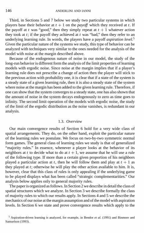
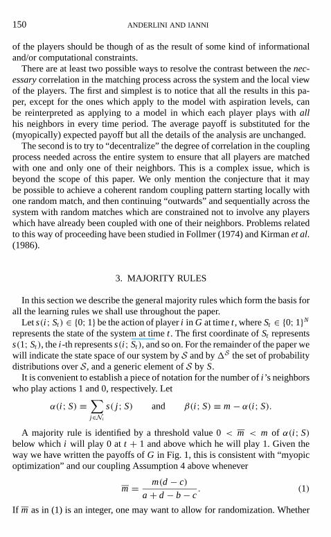
Time is discrete. At each datet = 1; . . .;∞, every playeri is coupled withone of his neighbors chosen at random in a way to be described shortly. Eachplayer then plays a simultaneous move two-by-two normal form game with theneighbor it has been coupled with. We denote this “underlying” game byG. WeassumeG to be symmetric. Therefore, in general,G can be written as in Fig. 1,where the two actions open to each player have been labeled 1 and 0, respectively.Many of the characterization results which we report below depend on specificassumptions on the values ofa, b, c, andd. We spell these out below. For thetime being we make one assumption onG which we maintain throughout the

148 ANDERLINI AND IANNI

FIGURE 1

paper. We assume thatG displays “strategic complementarities” in the followingsense of the term.

Assumption1. The expected payoff from playing1 (resp. 0) increases withthe probability that the opposing player pays1 (resp. 0). Moreover, both (1;1)and(0;0)are Nash equilibria of G. Formally,

a > c, b < d, a > b, and c< d.

The class of spatial structures we study can be conveniently thought of as aclass of graphs. A spatial arrangement of players and neighborhoods correspondsto a graph0 in which each player is represented by avertexof the graph and isconnected bym edgesto his neighboring players. Since a graph (undirected) inwhich each vertex is connected to exactlymedges is calledm-regular (Andrasfai,1977), we can state our first assumption on the spatial structure we study as thefollowing

Assumption2. The graph0 representing the spatial arrangements of theplayers and their neighbors is a finite m-regular graph.

We have said before that at each timet each player is coupled with one ofhis neighbors selected at random to play the underlying gameG. This clearlycannot be achieved by means of an independent draw for each player since ifi iscoupled withj , then j must be coupled withi , andi and j may have neighbors incommon. Again, matters become simpler if they are viewed in a graph-theoreticform. A 1-factor of0 is a subgraph3 of0 which contains the same vertices as0and a subset of its edges with the property that each vertex of3 is connected toexactly one edge. A 1-factor of0 clearly identifies one possible way to couple allplayers in a consistent way with one, and only one of their neighbors. Thereforethe random draw which determines the coupling of players att can be viewedas a random draw over the set of 1-factors of0.

We would like each player to be coupled with any of his neighbors withprobability exactly 1/m at each timet . We also must have “proper” couplingat each time in the sense that the coupling pattern of the entire system at eachdate is a 1-factor of0. It is known (Andrasfai, 1977) that some finitem-regulargraphs (with an even number of vertices) do not possess any 1-factor. Thereforewe need to make some extra assumptions on the spatial structure we study.

LEARNING FROM NEIGHBORS 149

A finite m-regular graph0 is theproductof m of its 1-factors{31; . . . ;3m}iff for any h andg, 3h and3g have no edges in common and the union of theedges of31 through to3m is exactly the set of edges of0. In this case0 is saidto admit the decomposition into the product of the 1-factors{31; . . . ;3m}.

It is clear that if0 admits at least one decomposition into the product ofm 1-factors, then by drawing at random one of the 1-factors of0 with equalprobability at each timet , we have a consistent way to couple all players whichguarantees that each playeri will play with any of his neighbors with equalprobability. Formally we state

Assumption3. The finite m-regular graph0 admits at least one decomposi-tion into the product of m1-factors, denoted by{31; . . . ;3m}.

It should be noted that Assumption 3 is a sufficient, but by no means necessary,condition for it to be possible to couple all the players with one and only one oftheir neighbors in an appropriate way.6

We are now ready to state our “working” assumption on coupling explicitly.We identify a complete coupling pattern throughout the system as one of the1-factors of0 as in Assumption 3 above. Letc(i ;3h) ∈ Ni be the neighbor withwhom i is coupled to play the game when the coupling pattern is3h.

Assumption4. At each time t, one of m1-factors of which0 is the productis drawn at random, with equal probability, defining a random variable3.Therefore, each and every player i is coupled to play G with one and only oneof his neighbors with equal probability. In other words,

Pr{c(i ; 3) = j } = 1/m, ∀i, ∀ j ∈ Ni .

We conclude this section with two observations. The first is that the decom-position of a graph into its 1-factors is in general not unique. Our results donot depend on which decomposition is chosen when more than one is available.The reason is that all that matters in our model is thatlocally the probability ofmatching a player with each of his neighbors be uniform. In other words, all weneed is that Assumption 4 above holds, and any decomposition0 into 1-factorswill be sufficient for this.

The second observation is that the random coupling process described inAssumption 4 exhibits a degree of “correlation” across the entire system.7 Thisis in contrast with the strictly local outlook which the players have of the model.These two features are obviously not in any logical contradiction with each othersince the coupling is essentially a move by Nature, whereas the local outlook

6 Sufficient conditions for Assumption 3 to hold are known, but necessary and sufficient conditionsfor a finitem-regular graph to have any 1-factor are quite complex indeed (Bollob´as, 1979).

7 We are grateful to an anonymous referee for raising this point and for suggesting a possible wayto handle the problem of “decentralized” coupling which we describe below.

150 ANDERLINI AND IANNI

of the players should be though of as the result of some kind of informationaland/or computational constraints.

There are at least two possible ways to resolve the contrast between thenec-essarycorrelation in the matching process across the system and the local viewof the players. The first and simplest is to notice that all the results in this pa-per, except for the ones which apply to the model with aspiration levels, canbe reinterpreted as applying to a model in which each player plays withallhis neighbors in every time period. The average payoff is substituted for the(myopically) expected payoff but all the details of the analysis are unchanged.

The second is to try to “decentralize” the degree of correlation in the couplingprocess needed across the entire system to ensure that all players are matchedwith one and only one of their neighbors. This is a complex issue, which isbeyond the scope of this paper. We only mention the conjecture that it maybe possible to achieve a coherent random coupling pattern starting locally withone random match, and then continuing “outwards” and sequentially across thesystem with random matches which are constrained not to involve any playerswhich have already been coupled with one of their neighbors. Problems relatedto this way of proceeding have been studied in Follmer (1974) and Kirmanet al.(1986).

3. MAJORITY RULES

In this section we describe the general majority rules which form the basis forall the learning rules we shall use throughout the paper.

Lets(i ; St) ∈ {0; 1} be the action of playeri in G at timet , whereSt ∈ {0; 1}Nrepresents the state of the system at timet . The first coordinate ofSt representss(1; St), thei -th representss(i ; St), and so on. For the remainder of the paper wewill indicate the state space of our system byS and by1S the set of probabilitydistributions overS, and a generic element ofS by S.

It is convenient to establish a piece of notation for the number ofi ’s neighborswho play actions 1 and 0, respectively. Let

α(i ; S) ≡∑j∈Ni

s( j ; S) and β(i ; S) ≡ m− α(i ; S).

A majority rule is identified by a threshold value 0< m < m of α(i ; S)below whichi will play 0 at t + 1 and above which he will play 1. Given theway we have written the payoffs ofG in Fig. 1, this is consistent with “myopicoptimization” and our coupling Assumption 4 above whenever

m= m(d − c)

a+ d − b− c. (1)

If m as in (1) is an integer, one may want to allow for randomization. Whether

LEARNING FROM NEIGHBORS 151

FIGURE 2

this type of randomization is allowed or not turns out to make a substantialdifference for the type of argument needed to show convergence of the systemto a steady state. We rule it out for the time being. Until Section 7 below we willsimply assume that the payoffs ofG are such that the threshold valuem is notan integer. The formal statement of a majority rule is now straightforward.

DEFINITION 1. A general majority rule with thresholdm is a mapMm: S 7→S such that, denoting byMm(i ; S) the i-th coordinate ofMm(S), we have

Mm(i ; S) ={

1 if α(i ; S) > m0 if α(i ; S) < m

.

To conclude this section we remark that it is very easy to think of examplesin which the dynamics of a majority rule donot converge. As we noted in theIntroduction, this is entirely due to the local nature of interaction in our model.

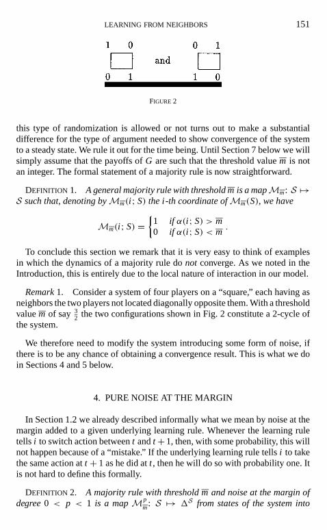
Remark1. Consider a system of four players on a “square,” each having asneighbors the two players not located diagonally opposite them. With a thresholdvaluem of say 3

2 the two configurations shown in Fig. 2 constitute a 2-cycle ofthe system.

We therefore need to modify the system introducing some form of noise, ifthere is to be any chance of obtaining a convergence result. This is what we doin Sections 4 and 5 below.

4. PURE NOISE AT THE MARGIN

In Section 1.2 we already described informally what we mean by noise at themargin added to a given underlying learning rule. Whenever the learning ruletells i to switch action betweent andt +1, then, with some probability, this willnot happen because of a “mistake.” If the underlying learning rule tellsi to takethe same action att + 1 as he did att , then he will do so with probability one. Itis not hard to define this formally.

DEFINITION 2. A majority rule with thresholdm and noise at the margin ofdegree0 < p < 1 is a mapMp

m: S 7→ 1S from states of the system into

152 ANDERLINI AND IANNI

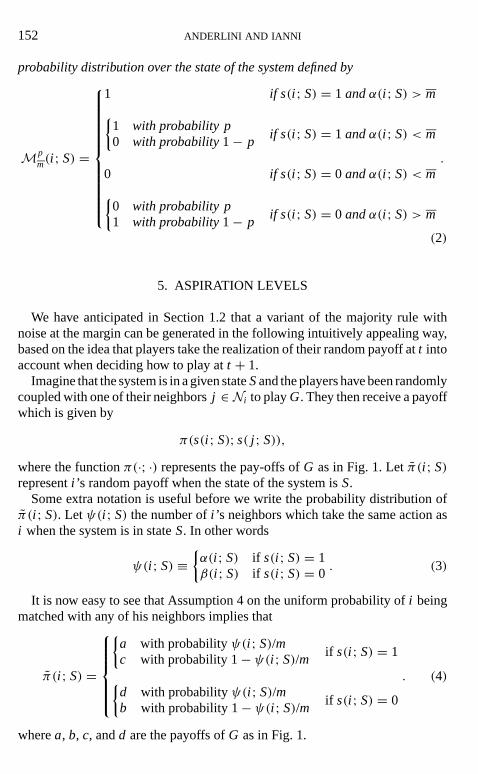
probability distribution over the state of the system defined by

Mpm(i ; S) =

1 if s(i ; S) = 1 andα(i ; S) > m{1 with probability p0 with probability1− p

if s(i ; S) = 1 andα(i ; S) < m

0 if s(i ; S) = 0 andα(i ; S) < m{0 with probability p1 with probability1− p

if s(i ; S) = 0 andα(i ; S) > m

.

(2)

5. ASPIRATION LEVELS

We have anticipated in Section 1.2 that a variant of the majority rule withnoise at the margin can be generated in the following intuitively appealing way,based on the idea that players take the realization of their random payoff att intoaccount when deciding how to play att + 1.

Imagine that the system is in a given stateSand the players have been randomlycoupled with one of their neighborsj ∈ Ni to playG. They then receive a payoffwhich is given by

π(s(i ; S); s( j ; S)),where the functionπ(·; ·) represents the pay-offs ofG as in Fig. 1. Letπ(i ; S)representi ’s random payoff when the state of the system isS.

Some extra notation is useful before we write the probability distribution ofπ(i ; S). Letψ(i ; S) the number ofi ’s neighbors which take the same action asi when the system is in stateS. In other words

ψ(i ; S) ≡{α(i ; S) if s(i ; S) = 1β(i ; S) if s(i ; S) = 0

. (3)

It is now easy to see that Assumption 4 on the uniform probability ofi beingmatched with any of his neighbors implies that

π(i ; S) =

{a with probabilityψ(i ; S)/mc with probability 1− ψ(i ; S)/m if s(i ; S) = 1

{d with probabilityψ(i ; S)/mb with probability 1− ψ(i ; S)/m if s(i ; S) = 0

. (4)

wherea, b, c, andd are the payoffs ofG as in Fig. 1.

LEARNING FROM NEIGHBORS 153

Given Assumption 1 on the payoffs ofG, it seems intuitively appealing to saythata andd are the “good” payoffs, whereasb andc are the “bad” payoffs ofG.The former are the payoffs received by the players when “coordination obtains,”while the latter are the payoffs to the players when “coordination fails.” Theintuition behind Definition 3 is that ifi gets a good payoff he will simply stickto the action previously taken. If a bad payoff is obtained then he will refer to anunderlying learning rule. In words, min{a; d} is the players’ payoffaspirationlevel.

We call a majority rule with a payoff aspiration level as just described amajority rule with payoff memory since it is the payoff in the last period whichdetermines the players’ behavior together with the local configuration of thesystem.

DEFINITION 3. A majority rule with thresholdm and payoff memory(or as-piration levels) is a mapAm: S 7→ 1S defined by

Am(i ; S) =

s(i ; S) if π(i ; S) ∈ {a; d}1 whenα(i ; S) > m

0 whenα(i ; S) < mif π(i ; S) ∈ {b; c} . (5)

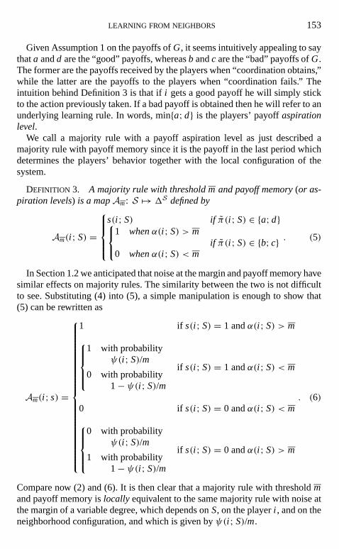
In Section 1.2 we anticipated that noise at the margin and payoff memory havesimilar effects on majority rules. The similarity between the two is not difficultto see. Substituting (4) into (5), a simple manipulation is enough to show that(5) can be rewritten as

Am(i ; s) =

1 if s(i ; S) = 1 andα(i ; S) > m1 with probability

ψ(i ; S)/m0 with probability

1− ψ(i ; S)/mif s(i ; S) = 1 andα(i ; S) < m

0 if s(i ; S) = 0 andα(i ; S) < m0 with probability

ψ(i ; S)/m1 with probability

1− ψ(i ; S)/mif s(i ; S) = 0 andα(i ; S) > m

. (6)

Compare now (2) and (6). It is then clear that a majority rule with thresholdmand payoff memory islocally equivalent to the same majority rule with noise atthe margin of a variable degree, which depends onS, on the playeri , and on theneighborhood configuration, and which is given byψ(i ; S)/m.

154 ANDERLINI AND IANNI

Two caveats apply to the similarity between noise at the margin and payoffmemory.8 The first thing we must be careful about is the possibility ofisolatedplayers. If at a particular state a player is “surrounded” by players who areplaying a strategy different from his own, then the probability that the playerwill achieve his aspiration payoff level is zero. This means that he will switchstrategy with probability one in the next period as opposed to switching with aprobability which is positive but strictly less than one in the noise at the margincase.

The second difficulty comes from the fact that a player will achieve his as-piration level payoff if and only if the neighboring player with whom he hasbeen coupled also achieves his aspiration level payoff. This creates a degree ofcorrelation in the noise induced by payoff memory which is not present in thecase of noise at the margin. The delicate case turns out to be the one in whichtwo players playing the same strategy are surrounded entirely by players whoplay a different strategy. In this case with payoff memory, eitherboth playerswill change strategy in the next period orneitherof them will. In the case ofnoise at the margin the same situation yields no switches, one switch, and twoswitches, all with strictly positive probability. Throughout the paper we will referto pairs of players whose local configuration is as above in a particular stateSas “isolated pairs atS.”

6. CONVERGENCE AND NASH EQUILIBRIUM

6.1. Absorbing States

In this section we prove convergence of the system to an absorbing state underthe dynamics specified by a majority rule with noise at the margin and with payoffmemory. The two arguments are similar and we start with the case of a majorityrule with noise at the margin.

By “the dynamics under a certain rule,” sayG: S 7→ 1S , we obviously meanthe finite Markov chain with state spaceS defined by the transition probabilitiesG(S), ∀S∈ S. In other words,∀S∈ S, we have thatG(S) can be interpreted asdefining the “row” of the transition matrix of the Markov chain associated withruleG. Given any ruleG we will indicate byM(G) the transition matrix of theMarkov chain associated withG.

The definition of absorbing states for the class of dynamical systems weconsider is now standard. It is convenient to define the set of absorbing states interms of “local stability.”

8 We are grateful to an anonymous referee for pointing out that the notion of “equivalence” betweennoise at the margin and payoff memory weused in an earlier version of the paper was mistaken.

LEARNING FROM NEIGHBORS 155

DEFINITION 4. Let a ruleG: S 7→ 1S be given.A player i is said to be locallystable(or just stable) at S underG if and only if, givenG and S, i is certain notto change strategy in the following period. In other words i is stable at S underG iff G(i ; S) = s(i ; S) with probability one. The set of stable players at S underG is denoted by V(S;G). The complement of V(S;G) in N is called the set ofunstable players at S underG, and is denoted by U(S;G). When there is no riskof ambiguity, G will be suppressed as an argument of V(·; ·) and U(·; ·).

DEFINITION 5. An absorbing(or stable) state for the dynamics under a givenruleG: S 7→ 1S is an S∈ S such thatG(S) = S with probability one. The set ofabsorbing states underG is denoted by A(G), when there is no risk of ambiguity,G will be suppressed as an argument of A(·). Moreover, it is clear that a state Sis absorbing underG if and only if all players are stable at S underG. In otherwords,

∀G, S∈ A(G)⇔ i ∈ V(S;G), ∀i = 1; . . . ; N.

6.2. Convergence to Absorbing States

The intuition behind the convergence results for the majority rules with noiseat the margin and payoff memory of the next two subsections is not difficult tooutline. To show that our Markov dynamics will converge to an absorbing statein finite time with probability one it is enough to show that all states of the systemcommunicate with some absorbing state with strictly positive probability in afinite number of periods. Consider now a nonabsorbing stateS∈ S. With obviousterminology we refer to the players who play action 1 atS as the 1-players atS, and to the others as the 0-players atS. Assume (without loss of generality upto a relabeling of strategies) that some 1-players are unstable atS. The noise atthe margin or the payoff memory ensures that any number 0≤ k ≤ ‖U (S;G)‖of9,10 unstable players may actually switch action in the following period. Wefollow the system along two “phases,” the first of which can be described asfollows. From S consider then the transition to a new stateS′ as follows.Allunstable 1-players atSplay action 0 atS′. All other players play the same actionat S′ as they did atS. FromS′ again change the action of all unstable 1-playersif there are any. We can then continue in this fashion until a stateS′′ is reachedat which either there are no 1-players left (in which case we have reached anabsorbing state) or all the 1 players are stable. Note that at this stage either all0-players are stable (in which case we have reached an absorbing state) or some0-players are unstable. Assume that the latter is the case.

9 Throughout the rest of the paper, we use the notation‖ · ‖ to denote the cardinality of a set.10 This statement is not strictly correct for the case of payoff memory. As we remarked at the end of

Section 5, in this case it is possible that our dynamical system forces at least one (isolated) or two ormore unstable players to switch action in the next period. However, the argument needs to be modifiedonly in a marginal way to take care of this point.

156 ANDERLINI AND IANNI

The second “phase” now involves transiting to a new state in which all theunstable 0 change their strategy to 1 and then repeating this operation in asymmetric way to what happened in phase one until either there are no 0-playersleft (in which case we are in an absorbing state) or all 0-players are stable. Oneobservation is now sufficient to see that the state we have reached at the end ofthe two phases must be absorbing. The fact that we are dealing with a majorityrule with a threshold level which is the same for all the players11 implies thatchanging the strategy of any number of unstable 1-players cannot create anyunstable 0-players and vice versa. Therefore, in phase two it cannot be that anyunstable 1-players are created by the change in strategy of any unstable 0-players.Since all 1-players are stable from the beginning of phase two, it follows thatallplayers are stable at the end of it.

We formalize our last observation as the following lemma.

LEMMA 1. Consider a majority rule with noise at the margin or with payoffmemory. Let S∈ S be an unstable state. Consider now a new state S′ in whichsome(or all) unstable1-players(unstable0-players) at S play strategy0 (1),and all other players play the same strategy at S′ as they did at S. Then(a) noneof the stable0-players(stable1-players) at S is unstable at S′ and(b) none of theplayers who change strategy who change strategy between S and S′ is unstableat S′.

Proof. We deal only with the case of unstable 1-players changing strategybetweenSandS′, since the other case is just a relabeling of this one.

Claim (a) is easily established noting that since going fromS to S′ only 1-players change their action to 0, it must be the case thatβ(i ; S′) ≥ β(i ; S),∀i = 1; . . . ; N. To see that (b) is correct notice that for a 1-playeri to beunstable atS it must be thatβ(i ; S) > m and that by the same argument as inthe proof of (a) we haveβ(i ; S′) ≥ β(i ; S). Therefore for any 1-playeri whichis unstable atS we haveβ(i ; S′) > m, and therefore after switching to 0,i isstable atS′.

6.3. Convergence with Noise at the Margin

We are now ready to state and prove our first convergence result. It saysthat the dynamics of a majority rule with noise at the margin converge to anabsorbing state in finite time with probability one. The proof follows the two-phase argument we informally described in Section 6.2 and appeals to Lemma 1above. The details are straightforward and hence the proof is omitted.

11 If the threshold value of the majority rule is interpreted as being determined by a “myopic bestreply,” assuming the threshold value to be uniform in the system is essentially the same as ruling outan underlying game which is asymmetric.

LEARNING FROM NEIGHBORS 157

THEOREM1. Consider the Markov chain yielded by a majority ruleMpm with

thresholdm and noise at the margin of degree p. Starting from any initial statethe system will find itself in an absorbing state in finite time with probability one.

6.4. Convergence with Payoff Memory

The second convergence result which we prove says that the dynamics definedby any majority rule with payoff memory will hit an absorbing state in finitetime with probability one. An argument very similar to the proof of Theorem 1applies to show convergence of the dynamics under the majority rule with payoffmemoryAm.

As we pointed out at the end of Section 5, a majority rule with payoff memoryis like a majority rule with noise at the margin of a variable degree. The twokey differences between the noise generated by payoff memory and noise at themargin arise in the cases of isolated players and of isolated pairs. Isolated playerschange action with probability one. Isolated pairs of players either both changeor both do not change action, all with positive probability.

The two-phase construction we have used to prove Theorem 1 relies on theflexibility which noise at the margin guarantees in the number of unstable playerswhich change action in the period following any unstable state of the system.Close inspection of the construction reveals that all is needed is that with strictlypositive probability none of the unstable players playing a particular strategychanges his action in the following period. Clearly, for these two features to holdwe need to exclude states with isolated players, while states with isolated pairspresent no problem. Inspection of (5) and (6) is enough to prove the following.

Remark2. Consider a majority rule with payoff memoryAm. Fix a strategys ∈ {0; 1}. Let Sbe an unstable state such that somes-players are unstable atS.Then we have that (a) the system transits with positive probability to a stateS′

in which all unstables-players change strategy and (b) if there are no isolateds-players, the system transits with strictly positive probability to a stateS′′ inwhich none of the unstables-players change strategy.

We are now ready to state and prove our second convergence result.

THEOREM2. Consider the Markov chain yielded by a majority ruleAm withthresholdm and payoff memory. Starting from any initial state the system willfind itself in an absorbing state in finite time with probability one.

Proof. As with Theorem 1, we need to show only that all states of the system“communicate” with some absorbing state with strictly positive probability in afinite number of steps.

Consider an arbitrary initial unstable stateS0. As usual we deal only withthe case in which some 1-players are unstable atS0; the other case is only arelabeling of this one.

158 ANDERLINI AND IANNI

Two cases are possible. Either the set of isolated 0-players atS0 is empty or itis not. If it is empty, start phase one and then phase two exactly as in the proofof Theorem 1. IfS0 contains some isolated 0-players, first transit toS1 changingthe strategy of all unstable 0-players and then start phase one and then phase twoexactly as in the proof of Theorem 1.

To prove Theorem 2 it is now sufficient to show that the transitions describedin phase one and phase two, starting from a state which contains no isolated0-players, all take place with strictly positive probability. If this is the case, theproof of Theorem 1 can be applied unchanged to the construction just described.By Remark 2, it is then sufficient to show that no isolated 0-players will appearalong the transitions of phase one and that no isolated 1-players will appearalong the transitions in phase two. By Lemma 1, all the 0-players created duringphase one are stable and therefore cannot be isolated. By Lemma 1 again, all the1-players created during phase two are stable and therefore cannot be isolatedeither. Since we start phase one after having changed the strategy of all isolated0-players (if any), this is enough to prove this claim.

6.5. Nash Equilibrium

We know from Theorems 1 and 2 that the locally interactive learning systemsdefined by a majority rule with noise at the margin or with payoff memoryconverge. Do we also know that they converge to a Nash equilibrium in someappropriate sense? The answer is yes.

TheN players with their fixed locations and neighbors defined by0, togetherwith the underlying gameG can be though of as defining anN-player game asfollows.

DEFINITION 6. Given a G and0 satisfying Assumptions1and3,we denote byG0 the following N-player game of incomplete information. First, Nature drawsone of the m1-factors of0 with equal probability. Then not having observedNature’s draw, all players i = 1; . . . ; N simultaneously decide which strategyin G to play. Let S∈ S be a strategy profile(which clearly is formally the sameobject as a state of the system so far). As a function of the state of Nature3h

and of S, player i ’s payoff in G0 is given by

5i (s(i ; S); S) = π(s(i ; S); s(c(i ;3h); S)),where c(i ;3h) is the neighbor with whom i is coupled when the coupling patternis3h, as defined in Section2.

The following formalizes our claim above about convergence to a Nash equi-librium.

Remark3. A state of the systemS ∈ S is an absorbing state for a majorityrule with thresholdm consistent with myopic optimization as in (1) and with

LEARNING FROM NEIGHBORS 159

noise at the margin or with payoff memory if and only if it is a Bayesian Nashequilibrium ofG0.

Proof. It is enough to notice that, by Definition 6, the expected payoff toiplayings ∈ {0; 1} when the strategy profile isS∈ S is simply

1

m

∑j∈Ni

π(s(i ; S); s( j ; S)), (7)

and therefore all players are stable if and only ifSis such that all players maximizetheir expected payoff as given by (7), given the strategy of other players.

6.6. “Mixed” Steady States

Before turning to a more specialized model in the next section, we would liketo conclude this part of the paper with a remark about the type of Nash equilibriawhich may emerge as a limit configuration of play of a locally interactive learningsystem like the one we have analyzed so far.

We have anticipated in Section 1.2 that, given the local nature of interaction,it is possible that only local coordination occurs. An example is sufficient todemonstrate this at this stage.12

Remark4. Let0 be described by the 8 vertices of a “cube” with each vertexhaving as neighbors the three vertices linked to it by an edge of the cube itself.Let the payoff ofG be given so that the myopic best-reply threshold ism= 3

2 asconsistent with (1). Then the strategy profileS in which the four players locatedon the “north face” of the cube play, say,s= 1, and the remaining players plays= 0, is a steady state of the majority learning rule with noise at the margin orwith payoff memory and therefore is also a Bayesian Nash equilibrium ofG0.

7. A SPECIAL STRUCTURE

In this section we specialize the model of Section 2 to a particular spatialstructure. Because we work with a particular type of graph0 we are able torelax the assumption we have made so far that the threshold level of the majorityrules considered should not be an integer. We will be able to allow for genuinerandomization in the underlying gameG.

The model we study is that of a rectangle with a lattice of horizontally andvertically aligned points which is then folded to form a Torus so that the “north”

12 It should be noted that in the “nonlocal” (a fully connected graph) version of our model it is stillpossible that “mixed” steady states occur. They correspond to the mixed strategy equilibrium of theunderlying gameG. The local nature of interaction in our model makes these mixed steady states bothrobust and more abundant than in the nonlocal case (cf. Section 8 below).

160 ANDERLINI AND IANNI

FIGURE 3

boundary of the rectangle is joined with the “south” boundary, while the “west”boundary is joined with the “east” boundary of the rectangle. Each player hasas neighbors the eight immediately adjacent players (vertically, horizontally, ordiagonally) to him on the Torus.13

Some of the arguments below use the details of the structure we study in thissection. Diagramatically, we will represent the structure as a grid of squares.Each player is represented by a square with the neighboring players being thesquares which have at least one edge or vertex in common with it.

Thus, one player called “Center” (C), with his eight neighbors “North” (N),“Northeast” (NE), “East” (E), “Southeast” (SE), and so on, and his neighbors’neighbors, can be pictured as in Fig. 3. From now on we will refer to the structurewe have just described, withN ≥ 12 players, simply as theN-Torus (recall thatN is assumed to be even throughout).

The first thing to notice is that Theorems 1 and 2 obviously apply to theN-Torus.

Remark5. When the players are arranged on anN-Torus, any majority rulewith threshold 0< m < 8 with noise at the margin of degreep or with payoffmemory converges as in Theorems 1 and 2.

We now specialize the payoffs of the underlying gameG to a particular casewhich allows us to investigate the effects of randomization inG and to charac-

13 The results contained in this section were first suggested by simulations carried out on a CAM-PChardware board, (Automatrix, Inc., Rexford, NY). The board simulates a Torus of size 256× 256players at a speed of 60 frames per second. The “neighborhood configuration” of the board can bealtered marginally from the one we have described, but is essentially fixed. The local updating rule, onthe other hand, is completely flexible and can be programmed by the user in a variant of the FORTH-83programming language. The programs we used are available from the authors on request. Cellularautomata have been extensively applied in many fields of research ranging from solid-state physicsto neurophysiology. For general up-to-date references see Toffoli and Margolus (1987) and Wuinscheand Lesser (1992).

LEARNING FROM NEIGHBORS 161

FIGURE 4

terize fully the steady states of the system in Section 8 below. For the remainderof the paper, unless we specify otherwise, we shall maintain the following

Assumption5. In addition to Assumption1, the payoffs of G satisfy d− c =a−b.Therefore, the two equilibria G are risk-equivalent in the sense of Harsanyiand Selten(1988).Moreover, by (1) it is clear that the thresholdm consistentwith myopic optimization is equal to12m= 4.

Notice that Assumption 5 doesnot imply that the two equilibria ofG are notPareto-rankable. From the point of view of exposition, however, there is no lossof generality in thinking of the payoffs ofG from now on as being given by thematrix shown in Fig. 4.

As with Remark 1, it is not difficult to see that the local nature of interaction inour model may prevent convergence of a majority rule dynamics on theN-Torusin the absence of noise.

Remark6. Consider theN-Torus withN = 16, with the following majorityrule. The threshold level ism= 4 and wheneverψ(i ; S) = 4, playeri random-izes between actions 0 and 1 with equal probability. Then the two configurationsshown in Fig. 5 clearly constitute a 2-cycle of the system.

The first learning rule which we investigate in detail is a majority rule withnoise at the margin, in which players randomize when exactly 4 neighbors playone strategy inG. We call this a majority rule with randomization and noise atthe margin.

FIGURE 5

162 ANDERLINI AND IANNI

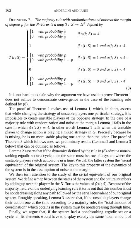
DEFINITION 7. The majority rule with randomization and noise at the marginof degree p for the N-Torus is a mapT : S 7→ 1S defined by

T (i ; S) =

{1 with probability 1

20 with probability 1

2

if α(i ; S) = 4

1 if s(i ; S) = 1 andα(i ; S) > 4{1 with probability p0 with probability1− p

if s(i ; S) = 1 andα(i ; S) < 4

0 if s(i ; S) = 0 andα(i ; S) < 4{0 with probability p1 with probability1− p

if s(i ; S) = 0 andα(i ; S) > 4

.

(8)

It is not hard to explain why the argument we have used to prove Theorem 1does not suffice to demonstrate convergence in the case of the learning ruledefined by (8).

The proof of Theorem 1 makes use of Lemma 1, which, in short, assertsthat while changing the strategy of unstable players one particular strategy, it isimpossible to create unstable players of the opposite strategy. In the case of amajority rule with randomization and noise at the margin Lemma 1 fails in thecase in whichψ(i ; S) = 4. In other words Lemma 1 fails when the unstableplayer to change action is playing a mixed strategy inG. Precisely because heis mixing, he is no more stable playing one action than the other. The proof ofTheorem 3 which follows uses two preliminary results (Lemma 2 and Lemma 3below) that can be outlined as follows.

Lemma 2 asserts that if the dynamics defined by the rule in (8) admit a nonab-sorbing ergodic set or a cycle, then the same must be true of a system where theunstable players switch actionone at a time. We call the latter system the “serialequivalent” of the original system. The key to this property of the dynamics ofthe system is in the assumption of noise at the margin.

We then turn attention to the study of the serial equivalent of our originalsystem. We define a map between the states of the system and the natural numbersby adding up over the players in theN-Torus the values ofψ(i ; S). Because of themajority nature of the underlying learning rule it turns out that this number mustbe nondecreasing along any path followed by the serial equivalent of our originalsystem. Roughly speaking, Lemma 3 asserts that, if the unstable players changetheir action one at the time according to a majority rule, the “total amount ofcoordination” which obtains in the system must be nondecreasing through time.

Finally, we argue that, if the system had a nonabsorbing ergodic set or acycle, all its elements would have to display exactly the same “total amount of

LEARNING FROM NEIGHBORS 163

coordination” as above. This is then shown to be impossible using the specificstructure of the Torus.

We start by defining formally the serial equivalent of our original system.

DEFINITION 8. Given a majority ruleT with randomization and noise at themargin of degree p for the N-Torus, its “serial equivalent” T ∗: S 7→ 1S isdefined as the system in which only one unstable player(drawn at random)changes action in G at any one time. Formally, given S∈ S, define the set H(S)of “serial successors” of S as

H(S) ≡ {S′ ∈ S | there exists a unique i∈ U (S) s.t. s(i ; S′) 6= s(i ; S)} (9)

whenever U(S) 6= ∅. Define also H(S) = S whenever U(S) = ∅. Then theserial equivalent ofT is defined by

T ∗(S) = S′ ∈ H(S) with probability1

‖ H(S) ‖ , ∀S′ ∈ H(S). (10)

LEMMA 2. If the Markov chain yielded by the learning ruleT has a nonab-sorbing ergodic set or a cycle, the same is true of the Markov chain yielded byits serial equivalentT ∗ (such nonabsorbing sets or cycles need not be the samefor both rules).

Proof. By inspection of (8), (9), and (10), a stateS∈ S is absorbing for thetransition matrixM(T ) if and only if it is absorbing forM(T ∗). Moreover, allzero entries ofM(T ) are also zero entries ofM(T ∗), and this is enough to provethe claim by standard results.

We now show that, along any path taken by the system yielded byT ∗, the“total amount of coordination” in theN-Torus cannot decrease. Let

9(S) ≡N∑

i=1

ψ(i ; S),

where, as in (3),ψ(i ; S) is the number ofi ’s neighbors who play the samestrategy asi at S. We then have

LEMMA 3. Let S0; . . . ; St ; . . . be any realization of the Markov chain yieldedbyT ∗ starting with any state S0. Then9(St+1) ≥ 9(St), ∀t = 0; 1; . . ..

Proof. By inspection of (8),

i ∈ U (S)⇔ ψ(i ; S) ≤ 4. (11)

164 ANDERLINI AND IANNI

For anyt consider nowtheplayeri ∈ U (S) such thats(i ; St) 6= s(i ; St+1). By(11) it is clear thatψ(i ; St+1) ≥ ψ(i ; St). By definition (3) ofψ(·; ·) it is alsoclear that∑

j∈Ni

ψ( j ; St+1) =∑j∈Ni

ψ( j ; St)+ 8− 2ψ(i ; St) ≥∑j∈Ni

ψ( j ; St). (12)

Sincei is the only player to change strategy betweenSt andSt+1, we have thatψ( j ; St+1) = ψ( j ; St)∀ j 6∈ Ni . Therefore, (11) and (12) are enough to provethe claim.

Our next step is to define the set of statesL(T ∗) which are not absorbing forT ∗ and such that the total amount of coordination9(S) cannot be increasedfurther in a finite number of transitions allowed by the transition matrixM(T ∗).Let M(T ∗)nSS′ be the standardn-step transition probability betweenS and S′

yielded byM(T ∗). Then we define

L(T ∗) ≡ {S 6∈ A(T ∗) |6 ∃S′ andn ≥ 1 such thatM(T ∗)nSS′ > 0

and9(S′) > 9(S)}. (13)

The last preliminary result we prove is that if the serial equivalent of ouroriginal system were to have a nonabsorbing ergodic set or a cycle, then thismust be contained inL(T ∗).

LEMMA 4. Suppose that a set of states C⊆ S were a nonabsorbing ergodicset or a cycle of the Markov chain yielded byT ∗. Then C⊆ L(T ∗).

Proof. By Lemma 3, we know that9(St) is nondecreasing witht alongany realization of the Markov chain. Notice that9(S) is bounded above by 8N(clearly9(S) = 8N, thenS is absorbing). Hence, starting from any initial stateS0, either the system communicates with an absorbing state in a finite number ofsteps or it communicates with at state inL(T ∗) (or both). Therefore all (if any)states which do not communicate with an absorbing state must communicatewith a state inL(T ∗). By standard results, this is enough to prove the claim.

We are now in a position to state and prove our first convergence result for theN-Torus.

THEOREM3. Consider the Markov chain yielded by the majority ruleT withrandomization and noise at the margin of degree of p for the N-Torus. Startingfrom any initial state the system will find itself in an absorbing state in finite timewith probability one.

Proof. From Lemma 2 we know that it is enough to show that the serial equiv-alent ofT admits no nonabsorbing ergodic subsets or cycles. From Lemma 4,

LEARNING FROM NEIGHBORS 165

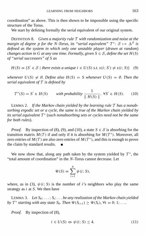
FIGURE 6

we know that it is then enough to show thatL(T ∗) = ∅. This is the line we willtake. We assume, by way of contradiction, thatL(T ∗) is not empty.

As a first step we characterize the local configuration of any unstable playerin any stateS ∈ L(T ∗). It turns out that only two are possible, and this will becrucial later in the argument.

Notice that, by definitionL(T ∗) we have

∀S∈ S, S∈ L(T ∗) andi ∈ U (S)⇒ ψ(i ; S) = 4, (14)

since otherwise9(S) could be increased by changingi ’s action inG and hencecontradict (13). It is also easy to see that the definition (13) ofL(T ∗) impliesthat∀ s ∈ L(T ∗), if i ∈ U (S) and j ∈ Ni play the same strategy atS then itmust be that

ψ( j ; S) ≥ 5; (15)

this is because if for somej ∈ Ni as above we hadj ∈ U (S), then by changingj ’s action first and theni ’s action as well, we could clearly achieve an increasein 9(·), but this is impossible sinceS∈ L(T ∗).

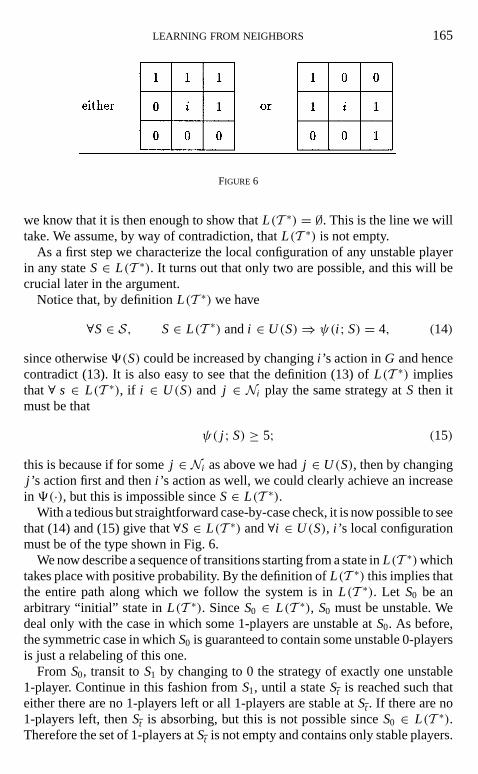
With a tedious but straightforward case-by-case check, it is now possible to seethat (14) and (15) give that∀S∈ L(T ∗) and∀i ∈ U (S), i ’s local configurationmust be of the type shown in Fig. 6.

We now describe a sequence of transitions starting from a state inL(T ∗)whichtakes place with positive probability. By the definition ofL(T ∗) this implies thatthe entire path along which we follow the system is inL(T ∗). Let S0 be anarbitrary “initial” state inL(T ∗). SinceS0 ∈ L(T ∗), S0 must be unstable. Wedeal only with the case in which some 1-players are unstable atS0. As before,the symmetric case in whichS0 is guaranteed to contain some unstable 0-playersis just a relabeling of this one.

From S0, transit toS1 by changing to 0 the strategy of exactly one unstable1-player. Continue in this fashion fromS1, until a stateSt is reached such thateither there are no 1-players left or all 1-players are stable atSt . If there are no1-players left, thenSt is absorbing, but this is not possible sinceS0 ∈ L(T ∗).Therefore the set of 1-players atSt is not empty and contains only stable players.

166 ANDERLINI AND IANNI

Choose now an arbitrary unstable 0-player atSt . Let this player be denoted byi t . Since all 1-players are stable atSt we know that ifi is a 1-player atSt , thenψ(i ; St) ≥ 5. Sincei t is unstable atSt , by (15) we also know that all 0-players inthe neighborhood ofi t are stable atSt . In other words, we know thati is the onlyunstable player in the entire neighborhood; formally, we know thatψ(i ; St) ≥ 5,∀i ∈ Ni t

.Transit now to a stateSt+1 by changing only the strategy ofi t to 1. Since before

the changei ’s local configuration must be as in Fig. 6, and all his neighbors mustbe stable, it is now possible to see with a case-by-case check (this simpler if wenotice that the configuration on the right-hand side of Fig. 6 is actually impossiblein this case) that one of the 0-players in the neighborhood ofi t must be unstable14

at St+1. Let this 0-player be denoted byi t+1.Clearly, the number of unstable neighbors ofi t+1 at St+1 is exactly one (namely

i t ). This is because all 1-players excepti t must be stable and because all 0-playersinNi t

must be stable by (15). Transit now fromSt+1 to a stateSt+2 by changingthe strategy ofi t+1 to 1. Sincei t+1 has exactly one unstable neighbor atSt+1, it ispossible, again with a case-by-case check (we use again the two configurationsin Fig. 6 and the observation that the configuration on the right-hand side isimpossible in this case), to verify that one 0-player in the neighborhood ofi t+1must be unstable atSt+2. Let this 0-player be denoted byi t+2.

Sincei t+1 ∈ Ni tit must be thati t is now stable atSt+2 (recall thati t is a

1-player atSt+1). Therefore, by the same arguments that applied toi t+1 at St+1we can conclude that exactly one player in the neighborhood ofi t+2 is unstableat St+2 (namelyi t+1).

We can now continue in this way to change to 1 the strategy of unstable 0-players created along the path without bound (note that the number of unstableneighbors of the unstable 0-players along the path is always exactly one). Sinceall the transitions we have described happen with strictly positive probability,this a contradiction. If we keep eliminating 0-players, we must eventually reachan absorbing state, but this is impossible since by definition no state inL(T ∗)communicates with an absorbing state in a finite number of steps. Therefore theassumption thatL(T ∗) is not empty leads to a contradiction and the proof iscomplete.

The last result of this section is a convergence theorem for theN-Torus whenthe learning rule is the majority rule with randomization and payoff memory (oraspiration levels). Since we have already discussed the role and interpretation ofadding payoff memory on a given learning rule in Section 5, we proceed directlywith a formal definition.

14 Recall that we are proceeding by contradiction. Therefore, if all the 0-players in the neighborhoodof i t are stable we already have a contradiction and there is nothing more to prove.

LEARNING FROM NEIGHBORS 167

DEFINITION 9. The majority rule with randomization and payoff memory forthe N-Torus is a mapP: S 7→ 1S defined by

P(i ; S) =

s(i ; S) if π(i ; S) ∈ {a; d}1 whenα(i ; S) > 40 whenα(i ; S) < 4{

1 with prob. 12

0 with prob. 12

whenα(i ; S) = 4if π(i ; S) ∈ {b; c}

.

(16)

As in Section 5, it is easy to see that by substituting the definition (4) ofπ(·; ·)into (16), the latter can then be viewed as the majority rule with randomizationand noise at the margin of a variable degree. We omit the algebra since this isroutine by now.

The two difficulties which arise in adapting the proof of Theorem 3 to the caseof payoff memory are related to isolated players and isolated pairs of players. Aswe remarked at the end of Section 5, all isolated players must change strategy inthe next period and isolated pairs change in pairs if they change at all. Thereforeit is clear that Definition 8 of serial equivalent does not adapt immediately tothe Markov chain byP. We modify it so that if there are isolated players and/orisolated pairs these all change strategy while all other players do not.

DEFINITION 10. The serial equivalentP is a mapP∗: S 7→ 1S obtainedfrom P in exactly the same way thatT ∗ is obtained fromT whenever S∈ Sdoes not contain isolated players or isolated pairs. Whenever S∈ S containsisolated players and/or isolated pairs, P∗ stipulates that the systems transitswith probability one to a new state S′ obtained from S by changing the strategyof all isolated players and all isolated pairs of players, while strategy of all otherplayers remains unchanged.

We now note that the total amount of coordination9(·)must be nondecreas-ing along any realization of the Markov chain given byP∗. The reasoning isexactly the same as in Lemma 3, plus the observation that changing the strategyof isolated players or of isolated pairs clearly increases9(·). For the sake ofcompleteness, without proof we state

LEMMA 5. Let S0; . . . ; St ; . . . be any realization of the Markov chain yieldedbyP∗ starting with any state S0. Then9(St+1) ≥ 9(St), ∀t = 0; 1; . . ..

As a last preliminary we note that if we defineL(P∗) in the same way asfor the case of noise at the margin, then the analogs of Lemmas 2 and 4 clearlyhold for the case of payoff memory. In other words, ifP admits a nonabsorbing

168 ANDERLINI AND IANNI

ergodic set or a cycle so doesP∗, and moreover any nonabsorbing ergodic setor cycle ofP∗ must be contained inL(P∗).

THEOREM4. Consider the Markov chain yielded by the majority ruleP withrandomization and payoff memory for the N-Torus.Starting from any initial statethe system will find itself in an absorbing state in finite time with probability one.

Proof. The argument is an adaptation of the proof of Theorem 2. Indeed,all that we need to notice is that ifS ∈ L(P∗), then clearlyψ(i ; S) ≥ 4,∀i = 1; . . . ; N; otherwise the value of9(·) could be increased violating thedefinition ofL(P∗). It follows that if S∈ L(P∗), Scannot contain any isolatedplayers or isolated pairs. Therefore the rest of the proof of Theorem 3 appliesunchanged to the case of payoff memory.

8. CHARACTERIZATION OF ABSORBING STATES

In this section we present a characterization of the possible steady states ofthe dynamics yielded by the twoN-Torus learning rules which we analyzed inthe previous section. Clearly, Remark 3 applies also to rulesT andP, so that thesteady states we characterize are the Nash equilibria of the appropriateN-playerincomplete information game.

The characterization of the steady states of the majority rule with random-ization and noise at the margin of payoff memory is very simple indeed. It isenough to notice that a stateScan be an absorbing state if and only if it is suchthat

ψ(i ; S) ≥ 5, ∀i = 1; . . . ; N.By a tedious but straightforward case-by-case check, it is then possible to

show that

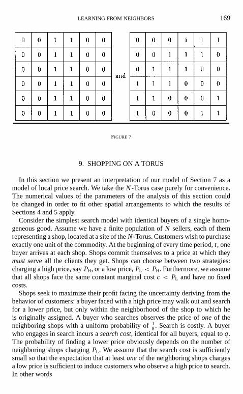
Remark7. There are two types of absorbing states for the rulesT andP fortheN-Torus. The first type is “homogeneous,” in which all players take the sameaction inG. The second type is “mixed,” in which some players take one actionand other players the other action available inG.

The mixed steady states can only be one of two forms. The first form is onein which the “boundary” between areas of theN-Torus in which one action isplayed is always a straight line (vertical or horizontal). In this case the minimum“thickness” of a set of players playing one particular action is 2. The second formis one in which the boundary between areas of theN-Torus in which one actionis played is always a 45◦ line (upward sloping or downward sloping). In this casethe minimum “thickness” of a set of players playing one particular action is 3.

Diagrammatic examples of the two possible forms of mixed steady states areshown in Fig. 7 (we “unfold” the entireN-Torus as a square).

LEARNING FROM NEIGHBORS 169

FIGURE 7

9. SHOPPING ON A TORUS

In this section we present an interpretation of our model of Section 7 as amodel of local price search. We take theN-Torus case purely for convenience.The numerical values of the parameters of the analysis of this section couldbe changed in order to fit other spatial arrangements to which the results ofSections 4 and 5 apply.

Consider the simplest search model with identical buyers of a single homo-geneous good. Assume we have a finite population ofN sellers, each of themrepresenting a shop, located at a site of theN-Torus. Customers wish to purchaseexactly one unit of the commodity. At the beginning of every time period,t , onebuyer arrives at each shop. Shops commit themselves to a price at which theymustserve all the clients they get. Shops can choose between two strategies:charging a high price, sayPH, or a low price,PL < PH. Furthermore, we assumethat all shops face the same constant marginal costc < PL and have no fixedcosts.

Shops seek to maximize their profit facing the uncertainty deriving from thebehavior of customers: a buyer faced with a high price may walk out and searchfor a lower price, but only within the neighborhood of the shop to which heis originally assigned. A buyer who searches observes the price ofoneof theneighboring shops with a uniform probability of1

8. Search is costly. A buyerwho engages in search incurs asearch cost, identical for all buyers, equal toq.The probability of finding a lower price obviously depends on the number ofneighboring shops chargingPL. We assume that the search cost is sufficientlysmall so that the expectation that at leastoneof the neighboring shops chargesa low price is sufficient to induce customers who observe a high price to search.In other words

170 ANDERLINI AND IANNI

Assumption6. The search cost q satisfies

0< q < 18(PH − PL).

We assume that the buyers correctly perceive the probability that search willresult in the observation of a low price as being equal to the fraction of neigh-boring shops actually chargingPL.15 The behavior of customers can thereforebe summarized as follows: (a) a buyer faced with a low price buys from the shophe is initially assigned to and (b) a buyer faced with a high price buys from theshop he is assigned to only if all the neighboring shops chargePH, and otherwisehe always pays the search costq and therefore observes the price of one of theneighboring shops drawn at random; if the neighbors drawn at random chargesstrictly less than the price initially observed, then the customer moves and buysfrom the cheaper shop.

Under these assumptions, by choosing the high-price strategy,PH, the shopwill get at mostone customer, whereas by charging the low price,PL, it willsellat leastone unit of product. It is evident that the expected payoff associatedwith a price strategy depends on the strategies adopted within the neighborhood.Intuitively, it is clear how a trade-off exists between selling more units at a lowprice and fewer units at a higher price. Since the maximum number of units thatany shop can possibly sell is limited by the number of neighboring shops (eight),the difference between the high price and the low price must not be too high tomake the model interesting. Formally we assume

Assumption7. The prices PH and PL are such that

13 PH < PL < PH. (17)

Let h(i ; S) be the number ofi ’s neighbors chargingPH when the system is instateS. Straightforward algebra shows that the expected payoffs,πE

H(i ; S) andπE

L (i ; S), associated with the two price strategies,PH andPL, are

πEH(i ; S) = (PH− c)

h(i ; S)8

and πEL (i ; S) = (PL − c)

(1− h(i ; S)

8

).

Given the values ofPH andPL, the precise point of balance between the twostrategies depends on the marginal costc. Therefore, by an appropriate choice ofc we can reproduce a majority rule behavior like the one described in Section 7.Formally we state

15 It may seem that we are endowing our shoppers with excessive “rationality” for a world in whichbehavior of other agents is dictated by myopic learning rules. We do this since it makes the steady statesof the dynamics we study in this section correspond to the Bayesian Nash equilibrium of an interestinggame as we will note below. The analysis we carry out here would, however, remain unchanged if weassumed that the buyers have some myopic probability of successful search in mind, and the searchcost is sufficiently low so as to ensure that all buyers who observe a high price engage in the costlysearch.

LEARNING FROM NEIGHBORS 171

Remark8. If (and only if)

c = (3PL − PH)

2, (18)

then the expected payoffs associated to the two price strategies,PH andPL, aresuch that

πEH(i ; S) ≥ πE

L (i ; S)⇔ h(i ; S) ≥ 4. (19)

It is useful to keep track of the actual probability distributions of profits andof profits per unit sold associated with the pricing strategies.

Remark9. The profits per unit sold whenc is as in (18) are32(PH − PL) forthe shops chargingPH and1

2(PH−PL) for the shops chargingPL. The probabilitydistribution over units sold for shops chargingPH is

1 with probabilityh(i ; S)/80 with probability(8− h(i ; S))/8

and for the shops chargingPL,16

(1+ k) with probability

(h(i ; S)

k

)(1

8

)k (7

8

)h(i ;S)−k

k = 0; . . . ; h(i ; S).

We denote the random payoff to shopi in stateS∈ S by π(i ; S).The dynamics we are interested in are the ones which arise from the shops

using the majority rule implicit in (19) with payoff memory. In other words, ifa shop’s profit does not fall below a given aspiration level which we choose tobe equal toPH− PL, then the shop will simply carry on charging the same pricewithout change. If, on the other hand, a shop’s profit falls belowPH − PL, thenthe price charged in the next period will be determined by a 4− 4 majority ruleconsistent with myopic profit maximization. We also assume that, when a shopis indifferent in expected terms between chargingPH andPL, the majority ruleinvolves randomization as in Section 7. Formally we have

DEFINITION 11. The majority learning rule with randomization and payoffmemory for the shopping model on the N-Torus is a mapQ: S 7→ 1S such that

T (i ; S) =

s(i ; S) if π(i ; S) ≥ (PH − PL)PH when h(i ; S) > 4PL when h(i ; S) < 4{

PH with prob. 12

PL with prob. 12

when h(i ; S) = 4if π(i ; s) < (PH − PL)

.

(20)

16 Note that ifh(i ; S) = 0 the formula below implies that the shop sells one unit with probabilityone.

172 ANDERLINI AND IANNI

Substituting the probability distribution of random payoffs given in Remark 9into (20) definingQ it is possible to see that the dynamics given byQ are a minormodification of the dynamics given byP for the N-Torus with randomizationand payoff memory. It is interesting to see precisely how this is the case.

Let us start with a shop chargingPH. If more than four neighboring shops alsochargePH, two cases are possible. The shop will sell either one unit or none (thelatter is possible only if some neighboring shop chargesPL and the customer’ssearch reveals this). If one unit is sold atPH the realized profit is more thanPH − PL and therefore the shop will keep chargingPH in the next period. If nounits are sold then the profit is zero, but since more than four neighbors chargePH the shop will keep chargingPH in the next period. If exactly four neighborschargePH, again either one unit is sold or no units are sold. If one unit is sold,the shop will keep chargingPH in the next period. If no units are sold, the shop’sprofit is below the aspiration levelPH − PL, and therefore the fact that exactlyfour neighbors chargePH will induce the shop to randomize betweenPH andPL with equal probability in the next period. The key feature of this case is thatoverall the shop will change toPL and will stick toPH both with strictly positiveprobability. If a shop chargingPH faces the wrong majority of shops chargingPL

but is not isolated, then again it will sell either one or zero units, both with strictlypositive probability. Therefore it will change toPL and stick toPH both withstrictly positive probability. A shop chargingPH which is isolated (surroundedby shops chargingPL) will lose its customers with probability one and thereforechange toPL with certainty in the next period. Notice that the behavior of isolatedpairs of shops surrounded by shops chargingPL is not perfectly correlated asin the case of payoff memory of Section 7. This is because it is possible thatone shop loses its customer to a cheaper shop but the other does not because thebuyer’s search reveals the only other high price in the neighborhood.

Consider now shops charging the low pricePL. Observe that shops chargingPL achieve their aspiration profit level ofPH − PL only if they sell two ormoreunits. Take the case of a shop chargingPL with more than four neighborschargingPL. It may sell one or more units (the latter is possible only if one ormore neighbors chargePH). If two or more units are sold, the aspiration level ofprofit is achieved and therefore the shop will keep chargingPL in the next period.If only one unit is sold (and it is interesting to notice that this will certainly bethe case if all the shop’s neighbors chargePL), the profit is belowPH − PL, butsince more than four shops in the neighborhood chargePL the shop will keepchargingPL in the next period. If precisely four neighbors of a shop chargingPL

also chargePL, then again one or more units may be sold. If only one unit is soldthe shop will randomize betweenPH and PL with equal probability in the nextperiod. If two or more units are sold the shop will keep chargingPL. Overall, theshop will change price and stay put both with positive probability. If more thanfour neighbors of a shop chargingPL charge the high pricePH, the shop willchange toPH with certainty if only one unit is sold and will stick toPL if two or

LEARNING FROM NEIGHBORS 173

more units are sold. Notice that one and two or more units will be sold all withstrictly positive probability in this case. This is true even in the case in which ashop chargingPL is isolated in the sense of having eight neighbors chargingPH.Therefore isolated shops chargingPL only change strategy with probability lessthan one. This is in contrast with the payoff memory rule of Section 7. Finally,notice that the behavior of isolated pairs of shops chargingPL is not perfectlycorrelated since one of them may get additional customers while the other doesnot.

From the discussion above it is clear that the dynamics given byQ are qualita-tively the same as those given byP, with the exception of isolated pairs of bothpricing strategies and of isolated shops chargingPL. A formal modification of theargument is not strictly needed, however. This is because underQ isolated pairsof players change strategy simultaneously with strictly positive probability, andall isolated players change strategy with strictly positive probability. Therefore,a modification of Definition 10 of the serial equivalent ofQ (although possible)is not needed. The proof of Theorem 4 applies unchanged to the following result.

COROLLARY 1. Consider the Markov chain given by the majority ruleQwith randomization and payoff memory for the shopping model on the N-Torus.Starting from any initial state, the system will converge to an absorbing state infinite time with probability one.

Once convergence is established, the equilibrium configuration are of partic-ular interest. Locally interactive systems provide a robust justification for pricedispersion in a search model.

Remark10. As in Remark 7 of Section 8, absorbing states for the shoppingmodel with local search on theN-Torus system may be “mixed.” This amountsto saying that, in the search model described above, the system might converge toan equilibrium configuration in which some shops chargePH and others chargePL. In other words, starting from a situation of completeex antehomogeneity(in costs, tastes, and behavior), locally interactive systems may give rise toheterogeneous pricing behavior. The characterization of such possible “mixed”steady states as in Fig. 6 in entirely determined by the specific spatial structureassumed.

It should be noted that, as in Remark 3, a steady state of the dynamics for theshopping model of this section can always be interpreted as a Bayesian Nashequilibrium of an associated game of incomplete information. The possibility ofequilibrium price dispersion in a search model is not a new result in the literature.However, equilibrium price dispersion has often been driven by some sort ofheterogeneity either in cost of production (Reinganum, 1979; MacMinn, 1982),in the search cost that consumers have to pay (Salop and Stiglitz, 1976, 1982),or in the propensity to search itself (Wilde and Schwartz, 1979). In contrast, weobtain equilibrium price dispersion in a model in which neither costs nor tastes

174 ANDERLINI AND IANNI

differ across agents. Our results also differ from those of Burdett and Judd (1983)in that we do not need to assume that search isnoisy, in the sense that one searchshot yields, with positive probability, more than one price observation for theconsumer.

10. CONCLUDING REMARKS

In this paper we investigate the long-run behavior of locally interactive learningsystems. We analyze the dynamics of a system in which a finite population ofplayers are randomly matched to play a two-by-two normal form game thatdisplaysstrategic complementarities. We assume players update their strategychoices following some general majority rules of behavior.

We observe that, in contrast to the obvious nonlocal analog of our system, thelocal nature of interaction in our model may prevent converence, yielding limitcycles in the absence of noise. This conforms to the findings of Berninghaus andSchwalbe (1992). A similar structure is also studied by Ellison (1993). In thisstudy convergence is obvious since a sufficient amount of noise is introducedin the system so as to ensure that it has a unique ergodic distribution. In thiscontext, Ellison (1993) finds that the local nature of interaction may yield higherspeed of convergence relative to nonlocal models such as that of Kandoriet al.(1993).

This paper concentrates on an “intermediate” level of noise in a locally in-teractive learning system. We introduce an assumption of “noise at the margin”which amounts to saying that a change of action triggers experimentation. Weare then able to show that the dynamical system with noise at the margin (and avariant of it in which players have payoff-based aspiration levels) converges to asteady state in finite time with probability one. In the particular case of playersarranged on a Torus we are able to demonstrate convergence with noise at themargin or payoff memory also when players are allowed genuine randomizationin case of “indifference.” Because of the nature of the noise in our model, thedynamics we study display a high degree of path dependence. Many steady statesare possible. In particular it is possible that in the long run only “local coordi-nation” occurs. We fully characterize the possible steady states of the system inthe special case of a Torus. Our model can also be interpreted as a model oflocalprice search. The steady states of the system in which only local coordinationoccurs demonstrate that the local nature of the interaction may be a robust reasonfor the existence ofequilibrium price dispersionin a search model.

We conclude with a question which naturally arises from this work and war-rants future attention. In short, “how likely” are the mixed steady states in whichtwo strategies coexist? The question can be divided into two more specific ones.The first is, given a particular initial distribution of strategies across the spatialstructure, how likely is the convergence to a mixed steady state? The second

LEARNING FROM NEIGHBORS 175

is, how wide is the range of initial distributions of strategies which allows con-vergence to a mixed steady state with positive probability or, more generally,how does the likelihood of mixed steady states change as we vary the initialdistribution of actions?

We do not have analytical answers, but cantentativelyreport some patternswhich emerged during simulations of a 256× 256 Torus (see footnote 13). Oursimulations all started with a random draw of strategy for each player with equalprobability and seem to give convergence to mixed steady states in roughly one-fifth of the cases (the vertical and horizontal boundaries being roughly twiceas likely as the diagonal ones). It should be strongly emphasized that thesepatterns are in our view to be treated with extreme caution because of substantialprogramming shortcuts we were forced to use. In the first place, the hardware weused made it impossible to obtain a proper coupling of players across the Torus.In essence, in our simulations each player played one of his neighbors randomly,regardless of whether that player had been coupled with another player or not.Moreover, for a structure with the order of 65,000 players it is extremely difficultto generate “enough noise” at sufficiently high speed. In order to introduce thenoise at the margin in the behavior of players, our simulations relied on “pseudo-noise” generated through a highly nonlinear rule unrelated to the system to besimulated.

REFERENCES

Allen, B. (1982a). “Some Stochastic Processes of Interdependent Demand and Technological Diffusionof an Innovation Exhibiting Externalities Among Adopters,”Int. Econ. Rev. 23, 595–607.

Allen, B. (1982b). “A Stochastic Interactive Model for the Diffusion of Information,”J. Math. Sociol.8, 265–281.

An, M. Y., and Kiefer, N. M. (1992). “Evolution and Equilibria Selection of Repeated Lattice Games,”mimeo. Cornell University.

An, M. Y., and Kiefer, N. M. (1993a). “A Dynamic Model of Local and Global Interactions amongEconomic Agents,” mimeo. Cornell University.

An, M. Y. and Kiefer, N. M. (1993b). “Local Externalities and Societal Adoption of Technologies,”mimeo. Cornell University.

Anderlini, L. (1989). “Some Notes on Church’s Thesis and the Theory of Games,”Theory Decision29, 19–52.

Anderlini, L., and Sabourian, H. (1993). “The Evolution of Computable Learning Rules,” mimeo.University of Cambridge.

Andrasfai, B. (1977).Introductory Graph Theory. Bristol: Hilger.

Bendor, J., Mookherjee, and Ray, D. (1991). “Aspiration-Based Adaptive Learning in Two PersonRepeated Games,” mimeo. Indian Statistical Institute.

Berninghaus, K. S., and Schwalbe, U. (1992). “Learning and Adaptation Processes in Games with aLocal Interaction Structure,” mimeo. University of Mannheim.

Binmore, K. (1987). “Modeling Rational Players, I,”Econ. Philos. 3, 179–214.

176 ANDERLINI AND IANNI

Binmore, K. (1988). “Modeling Rational Players, II,”Econ. Philos. 4, 9–55.

Binmore, K., and Samuelson, L. (1992). “Evolutionary Stability in Games Played by Finite Automata,”J. Econ. Theory57, 278–305.

Binmore, K., and Samuelson, L. (1993). “Muddling Through: Noisy Equilibrium Selection,” mimeo.University College London.

Blume, L. E. (1993). “The Statistical Mechanics of Strategic Interaction,”Games Econ. Behav. 5,387–424.

Bollobas, B. (1979).Graph Theory: An Introduction. New York: Springer.

Burdett, K., and Judd, K. L. (1983). “Equilibrium Price Dispersion,”Econometrica51, 955–969.

Canning, D. (1992a). “Rationality, Computability, and Nash Equilibrium,”Econometrica60, 877–888.

Canning, D. (1992b). “Average Behaviour in Learning Models,”J. Econ. Theory57, 442–472.

van Damme, E. (1987).Stability and Perfection of Nash Equilibria, Berlin: Springer-Verlag.

Durlauf, S. N. (1990). “Locally Interacting Systems, Coordination Failure and the Behavior of Aggre-gate Activity,” mimeo. Stanford University.

Ellison, G. (1993). “Learning, Local Interaction, and Coordination,”Econometrica61, 1047–1071.

Evans, R. (1992). “Out-of-Equilibrium Learning and Convergence to Nash Equilibrium,” mimeo.University of Cambridge.

Follmer, H. (1974). “Random Economies with Many Interacting Agents,”J. Math. Econ. 11, 1–13.

Freidlin, M., and Wentzell, A. (1984).Random Perturbations of Dynamical Systems. New York:Springer-Verlag.

Friedman, D. (1991). “Evolutionary Games in Economics,”Econometrica59, 637–666.

Fudenberg, D., and Kreps, D. (1990). “A Theory of Learning, Experimentation, and Equilibrium inGames,” mimeo. MIT.

Fudenberg, D., and Levine, D. K. (1993a). “Self-Confirming Equilibrium,”Econometrica61, 523–546.

Fudenberg, D., and Levine, D. K. (1993b). “Steady State Learning and Nash Equilibrium,”Economet-rica 61, 547–574.

Fudenberg, D., and Maskin, E. (1990). “Evolution and Cooperation in Noisy Repeated Games,”Amer.Econ. Rev. 80, 274–279.

Goyal, S., and Janssen, M. (1993). “Interaction Structure and The Stability of Conventions,” mimeo.Erasmus University, Rotterdam.

Harsanyi, J. C., and Selten, R. (1988).A General Theory of Equilibrium Selection in Games. Cambridge,MA: MIT Press.

Kandori, M., Mailath, G. J., and Rob, R. (1993). “Learning, Mutation, and Long Run Equilibria inGames,”Econometrica61, 29–56.

Kirman, A. (1992). “Variety: the Coexistence of Techniques,”Rev. Econ. Ind. 59, 65–79.

Kirman, A., Oddou, C., and Weber, S. (1986). “Stochastic Communication and Coalition Formation,”Econometrica54, 129–138.

MacMinn, R. D. (1982). “Search and Market Equilibrium,”J. Pol. Econ. 88, 308–315.

Mailath, G. J., Samuelson, L., and Shaked, A. (1993a). “Evolution with Endogenous Interactions,”mimeo. University of Bonn.

Mailath, G. J., Samuelson, L, and Shaked, A. (1993b). “Correlated Equilibria as Network Equilibria,”mimeo. University of Bonn.

Milgrom, P., and Roberts, J. (1990). “Rationalizability, Learning and Equilibrium in Games withStrategic Complementarities,”Econometrica58, 1225–1278.

LEARNING FROM NEIGHBORS 177

Milgrom, P., and Roberts, J. (1991). “Adaptive and Sophisticated Learning in Normal Form Games,”Games Econ. Behav. 3, 82–100.

Nachbar, J. H. (1990). “Evolutionary Selection Dynamics in Games: Convergence and Limit Proper-ties,” Int. J. Game Theory19, 59–90.

Reinganum, J. F. (1979). “A Simple Model of Equilibrium Price Dispersion,”J. Pol. Econ. 87, 851–858.

Salop, S., and Stiglitz, J. E. (1976). “Bargains and Rip-offs: A Model of Monopolistically CompetitivePrice Dispersion,”Rev. Econ. Stud. 44, 493–510.

Salop, S., and Stiglitz, J. E. (1982). “A Theory of Sales: A Simple Model of Equilibrium Price Dispersionwith Identical Agents,”Amer. Econ. Rev. 72, 1121–1130.

Selten, R. (1991). “Evolution, Learning, and Economic Behaviour,”Games Econ. Behav. 3, 3–24.

Toffoli, T., and Margolus, N. (1987).Cellular Automata Machines. Cambridge, MA: MIT Press.

Wilde, L. L., and Schwartz, A. (1979). “Equilibrium Comparison Shopping,”Rev. Econ. Stud. 46,543–554.

Wuinsche, A., and Lesser, M. (1992).The Global Dynamics of Cellular Automata. New York: Addison–Wesley.

Young, H. P. (1993). “The Evolution of Conventions,”Econometrica61, 57–84.