Wave-particle duality in multi-path interferometers: General concepts and three-path interferometers

arX

iv:0

710.

0179

v1 [

quan

t-ph

] 3

0 Se

p 20

07 WAVE-PARTICLE DUALITY IN MULTI-PATH

INTERFEROMETERS: GENERAL CONCEPTS AND

THREE-PATH INTERFEROMETERS

BERTHOLD-GEORG ENGLERT,1,2,∗ DAGOMIR KASZLIKOWSKI,1,2,†

LEONG CHUAN KWEK,1−3,‡ and WEI HUI CHEE1,§

1Department of Physics, National University of Singapore, Singapore 1175422Centre for Quantum Technologies, National University of Singapore, Singapore 1175433Nanyang Technological University, National Institute of Education, Singapore 259756

∗[email protected]†[email protected]

‡[email protected],[email protected]

§[email protected]

Received 30 September 2007

For two-path interferometers, the which-path predictability P and the fringe visibility Vare familiar quantities that are much used to talk about wave-particle duality in a quan-titative way. We discuss several candidates that suggest themselves as generalizationsP of P for multi-path interferometers, and treat the case of three paths in considerabledetail. To each choice for the path knowledge P , the interference strength V — thecorresponding generalization of V — is found by a natural, operational procedure. Inexperimental terms it amounts to finding those equal-weight superpositions of the pathamplitudes which maximize P for the emerging intensities. Mathematically speaking,one needs to identify a certain optimal one among the Fourier transforms of the stateof the interfering quantum object. Wave-particle duality is manifest, inasmuch as P = 1implies V = 0 and V = 1 implies P = 0, whatever definition is chosen. The possi-ble values of the pair (P, V ) are restricted to an area with corners at (P, V ) = (0, 0),(P, V ) = (1, 0), and (P, V ) = (0, 1), with the shape of the border line from (1, 0) to (0, 1)depending on the particular choice for P and the induced definition of V .

PACS : 03.65.Ta, 07.60.Ly

Keywords: Interferometers, wave-particle duality, path knowledge, interference strength

1. Introduction

Einstein’s wave-particle duality is arguably the most familiar phenomenon resulting

from Bohr’s principle of complementarity.a The intense debate between these two

protagonists, of which Bohr’s essay on the occasion of Einstein’s 70th birthday is

the best known public record,3 continues to be the object of scholarly studies,4

but there is, of course, rather wide-spread agreement by now on what used to be

controversial issues then.

aThis means a logical inference, not a historical one. In fact, the historical order is reversed: firstwave-particle duality (1905),1 then complementarity (1928).2

1

http://arxiv.org/abs/0710.0179v1

2 B.-G. Englert, D. Kaszlikowski, L. C. Kwek, and W. H. Chee

In the late 1920s and early 1930s, discussions of wave-particle duality focused on

the extreme situations where only the particle aspects are present, or only the wave

aspects. As natural as this focus may have been then, it does not do full justice to

the subject, as it ignores the intermediate situations in which both aspects of an

atomic system coexist within the boundaries that Nature imposes by the laws of

quantum mechanics.

The compromises that she permits are well understood in the context of two-

path interferometers, where various inequalities quantify to which extent wave and

particle properties can be observed simultaneously.b The historical example of the

Bohr-Einstein debate — Einstein’s version of Young’s double-slit interferometer,

with a recoiling first single slit — is familiar textbook material, but its literal

realization has not been achieved as yet.

What has become experimental reality, however, are analogous two-path inter-

ferometers of various kinds: for photons,9, 15–20 neutrons,7, 21 and atoms.22–24 They

enable quantitative studies of wave-particle duality, in which the said inequalities

are tested.c As expected, it is consistently found that the inequalities are obeyed,

not a single violation has been reported.

The basic inequality reads

P2 + V2 ≤ 1 ; (1)

all others can be derived from it with more or less sophisticated arguments.5 Here,

the predictability P quantifies the particle aspects: the a priori odds for guessing

the path right are given by 12 (1 + P), and the visibility V is simply the standard

fringe visibility, the quantitative measure for the wave aspect.

It is our primary objective in this paper to introduce, and discuss, the gener-

alization to multi-path interferometers, with a particular emphasis on three-path

interferometers where most features are already present in their generic forms. To

this end, we shall not employ Durr’s strategy of Ref. 25, who aimed at generaliza-

tions of P and V such that the equal sign in (1) continues to apply for all pure

states propagating through an n-path interferometer, as it does for two-path in-

terferometers. Rather, we consider a few possible choices for a generalization of Pthat suggest themselves and identify the corresponding generalization of V in, so

we think, a natural way.

Our present effort is not the first of its kind. We have already mentioned Durr’s

work,25 which is quite substantial, and an earlier discussion, rather brief and with no

definite conclusions, is contained in Ref. 12. We explore suggestions for generalizing

P from both. By contrast, the recent approach by Luis,26 who is motivated by the

experiment of Ref. 24, does not fit into our strategy; put tersely, he is concerned

with “this-path information” whereas we care for “which-path information.”

bThese matters are reviewed in Ref. 5, with a summary of the history of the subject in whichRefs. 6–13 play an important role. A technically simpler account, perhaps to be recommended asa first reading, is given in Ref. 14.cSome of the cited experiments are of a more qualitative nature, however.

Wave-particle duality in multi-path interferometers 3

Here is a brief outline. After presenting our general strategy in Sec. 2, we illus-

trate matters in the simple situation of two-path interferometers in Sec. 3. This is

followed by a detailed study of three-path interferometers in Sec. 4, which exhibit

the generic features of multi-path interferometers. Four-path interferometers and

multi-path interferometers are then briefly dealt with in Sec. 5. We close with a

summary.

2. General considerations

2.1. Operating an interferometer in particle mode or wave mode

In the most general terms, a n-path interferometer consists of an initial preparation

stage and a final probing stage, see Fig. 1. It is convenient to describe the state of

the interfering system between the stages by a n × n density matrix,

=

11 12 . . . 1n

21 22 . . . 2n

.... . .

...

n1 . . . nn

, ≥ 0 , tr {} = 1 . (2)

Of course, the diagonal entries 11, 22, . . . , nn are the probabilities of finding

the system in the 1st, 2nd, . . . , nth path, respectively. These probabilities are

experimentally available by operating the interferometer in the particle mode of

Fig. 1(a).

The wave mode of Fig. 1(b) probes the off-diagonal elements in (2). The unitary

n × n matrix F of the Fourier transformation,

→ ˜ = FF † , F † = F−1 , (3)

is such that all its matrix elements are of the same absolute size,

|Fjk| =1√n

, (4)

for which

Fjk =(

F−1)∗kj

=1√n

ei2πjk/neiφj + iϕk (5)

is the generic example, where φj and ϕk are arbitrary phases. If φj = 0 and ϕk = 0

for all j and k, we get the matrix of the standard discrete Fourier transformation.

The resulting probability of the mth detector to click is

˜mm =(

FF †)mm

=1

n+∑

j 6=k

FmjjkF ∗mk (6)

in general, and

˜mm =1

n+

1

n

∑

j 6=k

ei2πm(j − k)/nei(ϕj − ϕk)jk (7)


(a)

.......................................................................................................................

.

.

.

.

.

.

.

.

.

.

.

.

.

.

.

.

.

.

.

.

.

.

.

.

.

.

.

.

.

.

.

.

.

.

.

.

.

.

.

.

.

.

.

.

.

.

.

.

.

.

.

.

.

.

.

.

.

.

.

.

.

.

.

.

.

.

.

.

.

.

.

.

.

.

.

.

.

.

.

.

.

.

.

.

.

.

.

.

.

.

.

.

.

.

.

.

.

.

.

.

.

.

.

.

.

.

.

.

.

.

.

.

.

.

.

.

.

.

.

.

.

.

.

.

.

.

.

.

.

.

.

.

.

.

.

.

.

.

.

.

.

.

.

.

.

.

.

.

.

.

.

.

.

.

.

.

.

.

.

.

.

.

.

.

.

.

.

.

.

.

.

.

.

.

.

.

.

.

.

.

.

.

.

.

.

.

.

.

.

.

.

.

.

.

.

.

.

.

.

.

.

.

.

.

.

.

.

.

.

.

.

.

.

.

.

.

.

.

.

.

.

.

.

.

.

.

.

.

.

.

.

.

.

.

.

.

.

.

.

.

.

.

.

.

.

.

.

.

.

.

.

.

.

.

.

.

.

.

.

.

.

.

.

.

.

.

.

.

.

.

.

.

.

.

.

.

.

.

.

.

.

........................................................................................................................

.

.

.

.

.

.

.

.

.

.

.

.

.

.

.

.

.

.

.

.

.

.

.

.

.

.

.

.

.

.

.

.

.

.

.

.

.

.

.

.

.

.

.

.

.

.

.

.

.

.

.

.

.

.

.

.

.

.

.

.

.

.

.

.

.

.

.

.

.

.

.

.

.

.

.

.

.

.

.

.

.

.

.

.

.

.

.

.

.

.

.

.

.

.

.

.

.

.

.

.

.

.

.

.

.

.

.

.

.

.

.

.

.

.

.

.

.

.

.

.

.

.

.

.

.

.

.

.

.

.

.

.

.

.

.

.

.

.

.

.

.

.

.

.

.

.

.

.

.

.

.

.

.

.

.

.

.

.

.

.

.

.

.

.

.

.

.

.

.

.

.

.

.

.

.

.

.

.

.

.

.

.

.

.

.

.

.

.

.

.

.

.

.

.

.

.

.

.

.

.

.

.

.

.

.

.

.

.

.

.

.

.

.

.

.

.

.

.

.

.

.

.

.

.

.

.

.

.

.

.

.

.

.

.

.

.

.

.

.

.

.

.

.

.

.

.

.

.

.

.

.

.

.

.

.

.

.

.

.

.

.

.

.

.

.

.

.

.

.

.

.

.

.

.

.

.

.

.

.

.

.

.

....................................

.

.

.

.

.

.

.

.

.

.

.

.

.

.

.

.

.

g

e

n

e

r

a

l

i

z

e

d

b

e

a

m

s

p

l

i

t

t

e

r

...........................................................

............................................. ...........................................................

............................................. ...........................................................

.

.

.

............................................. ...........................................................

.................................................................................................................................................................................................................................................................................................................................................................

path 1

.................................................................................................................................................................................................................................................................................................................................................................

path 2

.................................................................................................................................................................................................................................................................................................................................................................

path 3

.

.

.

.................................................................................................................................................................................................................................................................................................................................................................

path n

................................

.

.

.

.

.

.

.

.

.

.

.

.

.

.

.

.

.

.

.

.

......

.

.

.

.

.

.

.

.

.

.

.

.

.

.

.

.

.

.

.

.

.

.

.

.

.

.

.

.

.

.

.

....

D

1

................................

.

.

.

.

.

.

.

.

.

.

.

.

.

.

.

.

.

.

.

.

......

.

.

.

.

.

.

.

.

.

.

.

.

.

.

.

.

.

.

.

.

.

.

.

.

.

.

.

.

.

.

.

.

...

D

2

................................

.

.

.

.

.

.

.

.

.

.

.

.

.

.

.

.

.

.

.

.

......

.

.

.

.

.

.

.

.

.

.

.

.

.

.

.

.

.

.

.

.

.

.

.

.

.

.

.

.

.

.

.

.

...

D

3

.

.

.

...............................

.

.

.

.

.

.

.

.

.

.

.

.

.

.

.

.

.

.

.

.

.

.......

.

.

.

.

.

.

.

.

.

.

.

.

.

.

.

.

.

.

.

.

.

.

.

.

.

.

.

.

.

.

....

D

n

(b)

.......................................................................................................................

.

.

.

.

.

.

.

.

.

.

.

.

.

.

.

.

.

.

.

.

.

.

.

.

.

.

.

.

.

.

.

.

.

.

.

.

.

.

.

.

.

.

.

.

.

.

.

.

.

.

.

.

.

.

.

.

.

.

.

.

.

.

.

.

.

.

.

.

.

.

.

.

.

.

.

.

.

.

.

.

.

.

.

.

.

.

.

.

.

.

.

.

.

.

.

.

.

.

.

.

.

.

.

.

.

.

.

.

.

.

.

.

.

.

.

.

.

.

.

.

.

.

.

.

.

.

.

.

.

.

.

.

.

.

.

.

.

.

.

.

.

.

.

.

.

.

.

.

.

.

.

.

.

.

.

.

.

.

.

.

.

.

.

.

.

.

.

.

.

.

.

.

.

.

.

.

.

.

.

.

.

.

.

.

.

.

.

.

.

.

.

.

.

.

.

.

.

.

.

.

.

.

.

.

.

.

.

.

.

.

.

.

.

.

.

.

.

.

.

.

.

.

.

.

.

.

.

.

.

.

.

.

.

.

.

.

.

.

.

.

.

.

.

.

.

.

.

.

.

.

.

.

.

.

.

.

.

.

.

.

.

.

.

.

.

.

.

.

.

.

.

.

.

.

.

.

.

.

.

.

.

........................................................................................................................

.

.

.

.

.

.

.

.

.

.

.

.

.

.

.

.

.

.

.

.

.

.

.

.

.

.

.

.

.

.

.

.

.

.

.

.

.

.

.

.

.

.

.

.

.

.

.

.

.

.

.

.

.

.

.

.

.

.

.

.

.

.

.

.

.

.

.

.

.

.

.

.

.

.

.

.

.

.

.

.

.

.

.

.

.

.

.

.

.

.

.

.

.

.

.

.

.

.

.

.

.

.

.

.

.

.

.

.

.

.

.

.

.

.

.

.

.

.

.

.

.

.

.

.

.

.

.

.

.

.

.

.

.

.

.

.

.

.

.

.

.

.

.

.

.

.

.

.

.

.

.

.

.

.

.

.

.

.

.

.

.

.

.

.

.

.

.

.

.

.

.

.

.

.

.

.

.

.

.

.

.

.

.

.

.

.

.

.

.

.

.

.

.

.

.

.

.

.

.

.

.

.

.

.

.

.

.

.

.

.

.

.

.

.

.

.

.

.

.

.

.

.

.

.

.

.

.

.

.

.

.

.

.

.

.

.

.

.

.

.

.

.

.

.

.

.

.

.

.

.

.

.

.

.

.

.

.

.

.

.

.

.

.

.

.

.

.

.

.

.

.

.

.

.

.

.

.

.

.

.

.

.

....................................

.

.

.

.

.

.

.

.

.

.

.

.

.

.

.

.

.

g

e

n

e

r

a

l

i

z

e

d

b

e

a

m

s

p

l

i

t

t

e

r

...........................................................

............................................. ...........................................................

............................................. ...........................................................

.

.

.

............................................. ...........................................................

.................................................................................................................................................................................................................................................................................................................................................................

path 1

.................................................................................................................................................................................................................................................................................................................................................................

path 2

.................................................................................................................................................................................................................................................................................................................................................................

path 3

.

.

.

.................................................................................................................................................................................................................................................................................................................................................................

path n

.......................................................................................................................

.

.

.

.

.

.

.

.

.

.

.

.

.

.

.

.

.

.

.

.

.

.

.

.

.

.

.

.

.

.

.

.

.

.

.

.

.

.

.

.

.

.

.

.

.

.

.

.

.

.

.

.

.

.

.

.

.

.

.

.

.

.

.

.

.

.

.

.

.

.

.

.

.

.

.

.

.

.

.

.

.

.

.

.

.

.

.

.

.

.

.

.

.

.

.

.

.

.

.

.

.

.

.

.

.

.

.

.

.

.

.

.

.

.

.

.

.

.

.

.

.

.

.

.

.

.

.

.

.

.

.

.

.

.

.

.

.

.

.

.

.

.

.

.

.

.

.

.

.

.

.

.

.

.

.

.

.

.

.

.

.

.

.

.

.

.

.

.

.

.

.

.

.

.

.

.

.

.

.

.

.

.

.

.

.

.

.

.

.

.

.

.

.

.

.

.

.

.

.

.

.

.

.

.

.

.

.

.

.

.

.

.

.

.

.

.

.

.

.

.

.

.

.

.

.

.

.

.

.

.

.

.

.

.

.

.

.

.

.

.

.

.

.

.

.

.

.

.

.

.

.

.

.

.

.

.

.

.

.

.

.

.

.

.

.

.

.

.

.

.

.

.

.

.

.

.

.

.

.

.

.

........................................................................................................................

.

.

.

.

.

.

.

.

.

.

.

.

.

.

.

.

.

.

.

.

.

.

.

.

.

.

.

.

.

.

.

.

.

.

.

.

.

.

.

.

.

.

.

.

.

.

.

.

.

.

.

.

.

.

.

.

.

.

.

.

.

.

.

.

.

.

.

.

.

.

.

.

.

.

.

.

.

.

.

.

.

.

.

.

.

.

.

.

.

.

.

.

.

.

.

.

.

.

.

.

.

.

.

.

.

.

.

.

.

.

.

.

.

.

.

.

.

.

.

.

.

.

.

.

.

.

.

.

.

.

.

.

.

.

.

.

.

.

.

.

.

.

.

.

.

.

.

.

.

.

.

.

.

.

.

.

.

.

.

.

.

.

.

.

.

.

.

.

.

.

.

.

.

.

.

.

.

.

.

.

.

.

.

.

.

.

.

.

.

.

.

.

.

.

.

.

.

.

.

.

.

.

.

.

.

.

.

.

.

.

.

.

.

.

.

.

.

.

.

.

.

.

.

.

.

.

.

.

.

.

.

.

.

.

.

.

.

.

.

.

.

.

.

.

.

.

.

.

.

.

.

.

.

.

.

.

.

.

.

.

.

.

.

.

.

.

.

.

.

.

.

.

.

.

.

.

.

.

.

.

.

.

a

n

y

a

r

b

i

t

r

a

r

y

F

o

u

r

i

e

r

t

r

a

n

s

f

o

r

m

........................................................... ...........................................................

........................................................... ...........................................................

........................................................... ...........................................................

........................................................... ...........................................................

...............................

.

.

.

.

.

.

.

.

.

.

.

.

.

.

.

.

.

.

.

.

.

.....

.

.

.

.

.

.

.

.

.

.

.

.

.

.

.

.

.

.

.

.

.

.

.

.

.

.

.

.

.

.

.

.

....

D

1

...............................

.

.

.

.

.

.

.

.

.

.

.

.

.

.

.

.

.

.

.

.

.

.......

.

.

.

.

.

.

.

.

.

.

.

.

.

.

.

.

.

.

.

.

.

.

.

.

.

.

.

.

.

.

....

D

2

................................

.

.

.

.

.

.

.

.

.

.

.

.

.

.

.

.

.

.

.

.

......

.

.

.

.

.

.

.

.

.

.

.

.

.

.

.

.

.

.

.

.

.

.

.

.

.

.

.

.

.

.

.

....

D

3

.

.

.

...............................

.

.

.

.

.

.

.

.

.

.

.

.

.

.

.

.

.

.

.

.

.

.

....

.

.

.

.

.

.

.

.

.

.

.

.

.

.

.

.

.

.

.

.

.

.

.

.

.

.

.

.

.

.

.

.

.

...

D

n

preparation stageprobing stage

.................................................................................................................................................................................................................................................................................................................................................................................................................................................... .....................................................................................................................................................................................................................................................................................................................................................................................................................................................

.

.

.

.

.

.

.

.

.

.

.

.

.

.

.

.

.

.

.

.

.

.

.

.

.

.

.

.

.

.

.

.

.

.

.

.

.

.

.

.

.

.

.

.

.

.

.

.

.

.

.

.

.

.

.

.

.

.

.

.

.

.

.

.

.

.

.

.

.

.

.

.

.

.

.

.

.

.

.

.

.

.

.

.

.

.

.

.

.

.

.

.

.

.

.

.

.

.

.

.

.

.

.

.

.

.

.

.

.

.

.

.

.

.

.

.

.

.

.

.

.

.

.

.

.

.

.

.

.

.

.

.

.

.

.

.

.

.

.

.

.

.

.

Fig. 1. The two stages of a n-path interferometer: preparation stage and probing stage, andthe two modes of operation: particle mode and wave mode. Left side: At the preparation stage,the incoming intensity (usually only one input port is used) is distributed over all paths by a“generalized beam splitter” or nitter, which is the n-port version of the entry beam splitter of thecommon two-path interferometers. A symmetric nitter is unbiased and assigns equal intensity toall paths (analogous to a symmetric 50:50 beam splitter), but it is more general to allow for abiased transformation (an asymmetric beam splitter in the case of n = 2), so that the intensitymay vary from one path to the next. Right side: (a) In particle mode (top), the probing justamounts to detecting the path, a click of detector Dm indicating that the mth path was the case.(b) In wave mode (bottom), the probing stage uses a Fourier transformation, that is: a symmetricnitter, in front of the detectors, so that all paths contribute equally to the intensity in each ofthe n output ports. In principle, any arbitrary Fourier transformation is to be considered, but inpractice a suitably chosen set of n transformations suffice, each characterized by the values of therelative phases between the amplitudes of the paths. The differences in the probabilities that thevarious detectors D1, D2, . . . , Dn respond result only from these relative phases. Taken together,the probabilities constitute the potentially complicated interference pattern, in their dependenceon those relative phases.

in particular for the generic F of (5), where the phases φj are irrelevant in this

context.

We must not fail to note that, as a consequence of the defining property (4) of the


general Fourier transform, the two modes of operation in Fig. 1 are complementary.

For, if the path is certain in particle mode, that is: mm = δmm′ if the m′th

path is the case, then all detectors will click with equal probability in wave mode:

˜mm = 1/n. And conversely, if ˜mm = δmm′ for one Fourier transform in Fig. 1(b),

then mm = 1/n follows, so that all paths are found with equal probability in

Fig. 1(a).

2.2. Fourier matrices

What is hinted at in Eq. (5) can be carried out for any Fourier matrix,

F =

eiφ1 0 . . . 0

0 eiφ2 . . . 0...

. . ....

0 . . . eiφn

1√n

· · · · · · · 1...

. . . 1...

. . ....

1 1 . . . 1

eiϕ1 0 . . . 0

0 eiϕ2 . . . 0...

. . ....

0 . . . eiϕn

, (8)

where the input phases ϕk and the output phases φj are pulled out such that the

central Fourier matrix has elements 1/√

n in the nth row and the nth column. Only

n − 1 of these 2n phases are relevant because the ˜mms do not involve the output

phases φk, and the option to redefine all phases jointly in accordance with

φj → φj + α , ϕk → ϕk − α (α arbitrary) (9)

can be used to set, say, ϕn = 0 by convention.

For n = 2 this gives a unique central Fourier matrix,

F =1√2

(

−1 1

1 1

)

, (10)

and for n = 3 there are two possible central Fourier matrices,

F =1√3

ei2π/3 e−i2π/3 1

e−i2π/3 ei2π/3 1

1 1 1

and F =

1√3

e−i2π/3 ei2π/3 1

ei2π/3 e−i2π/3 1

1 1 1

, (11)

but these two are equivalent for our purposes because they differ only by a permu-

tation of rows, that is: of the output channels, which can be compensated for by a

relabeling of the detectors in Fig. 1(b).

For n = 4, we have a one-parametric family of possible central Fourier matrices,

F =1

2

eit −1 −eit 1

−1 1 −1 1

−eit −1 eit 1

1 1 1 1

with arbitrary real t , (12)

supplemented by those matrices that one obtains by permutations of columns that

cannot be undone by permuting rows. The Fourier matrix of (5) corresponds to


t = π/2, and t = 0 in conjunction with permuting the 2nd and 3rd rows gives the

tensor product of the 2 × 2 matrix in (10) with itself.

For n = 5, the situation is similar to that for n = 3, as there is essentially

only one central Fourier matrix, the standard one of (5). Unfortunately, this is not

true for other prime values of n. For example, there are five inequivalent choices

for n = 7. And for composite values of n, we have continuous families of central

Fourier matrices, is illustrated above for n = 4 = 2 × 2; more about this at the

website of Ref. 27.

Our choice of terminology to refer to all matrices with the property (4) as

Fourier matrices is not everybody’s convention. Some authors speak of Hadamard

matrices instead,d thus generalizing the real Hadamard matrices of combinatorics

which have ±1 as matrix elements — such as the 2 × 2 matrix in (10) or the

t = 0 version of the 4 × 4 matrix in (12) — to complex matrices, and our central

Fourier matrices of (8) are called dephased Hadamard matrices. Unfortunately, the

general parameterization of all Fourier or Hadamard n × n matrices is not known

for arbitrary values of n. A concise guide is Ref. 28, and a catalog of known cases

up to n = 16 is available at the web site maintained, in a truly commendable effort,

by Zyczkowski and Tadej,27 where one also finds an extensive list of references on

the subject.

From the point of view of quantum physics, the elements of a Fourier matrix are

the transition amplitudes between two mutually unbiased bases. Accordingly, the

particle-mode and the wave-mode operation of the n-path interferometer in Fig. 1

realize the measurements of a pair of complementary observables, as we noted at

the end of Sec. 2.1. In this context one usually encounters Fourier transformations,

and this prompted our choice of terminology.

2.3. Quantification of the path knowledge

Path knowledge is knowledge about the probabilities for detector clicks in Fig. 1(a),

that is: knowledge about the diagonal elements of the density matrix in (2). In

view of the normalization of to unit trace, one needs n − 1 real parameters to

specify all mm. For example, the real and imaginary parts of the complex numbers

z1, z2, . . . , zn−1 that are defined by

zk =n∑

m=1

ei2πkm/nmm = z∗n−k (13)

may serve this purpose. Clearly, then, there cannot be a unique universal way of

quantifying path knowledge by a single number (except for n = 2), and various

numerical measures will be justifiable. To a considerable extent, it thus remains a

dBy convention, Fourier matrices are unitary, F−1 = F †, whereas Hadamard matrices are nor-malized to unit-modulus matrix elements, such that nH−1 = H†, and corresponding matrices arerelated by H =

√nF .


matter of taste, or convenience, for which of them to opt, unless particular circum-

stances leave no choice.

We shall regard any continuous function P (diag) ≡ P (11, 22, . . . , nn) of the

diagonal elements of as an acceptable measure of path knowledge, and thus as

a valid generalization of the two-path predictability P , if it meets these natural

criteria:a. P = 1 if mm = 1 for one m, i.e., if the path is certain, and only

then.

b. P = 0 if mm = 1/n for all m, i.e., if the path is completely

uncertain.

c. P must be invariant under permutations of the diagonal elements

of .

d. P must be convex, that is:

P (diag) ≤ (1 − λ)P (diag1) + λP (diag2)

with = (1−λ)1 +λ2 and 0 ≤ λ ≤ 1 holds for any two density

matrices 1 and 2.

e. Any degradation of the mms, that is: the increase of a smaller

one at the expense of a larger one, must not increase the value

of P .

(14)

Property (14e) is actually implied by property (14d), but we list it nevertheless be-

cause it is a weaker version of Durr’s fourth criterion, at Eq. (1.14) in Ref. 25, which

requires “should decrease” rather than “must not increase.” The other properties

are equivalent to Durr’s.

2.3.1. First example: Betting on the path

At Eq. (1), we recalled that the standard predictability P of two-path interfer-

ometers is essentially the odds for guessing the way right. More generally, then,

a path-knowledge function P (diag) can be associated with a given set of betting

rules, and this will serve as our first example.

Whereas there is really only one kind of bet for n = 2, there is a variety of pos-

sible bets in n-path interferometers. We consider bets of the following construction.

If you guess the path right on the 1st try, you win g1 = 1 unit. If

your 1st guess is wrong, but your 2nd is right, you win g2 units.

And so forth: If you need m guesses, you win gm units, and if all

your n − 1 guesses are wrong, you win gn units (which will be a

negative amount, so that you actually lose).

(15)

The amount won should be the larger, the fewer guesses you need, and a random

guess should have a neutral over-all return. These natural requirements impose the

restrictions

1 = g1 > g2 ≥ g3 ≥ . . . ≥ gn ,

n∑

m=1

gm = 0 . (16)


The optimal betting strategy is clearly to first bet on the most likely path, then

on the second likely, and so on. On average, the gain is then

Pbet =

n∑

m=1

gmpm , (17)

where the pms are the mms in descending order,{

p1, p2, . . . , pn

}

={

11, 22, . . . , nn

}

, p1 ≥ p2 ≥ . . . ≥ pn ≥ 0 . (18)

By construction, Pbet meets the criteria (14a–e), and so Pbet is an acceptable nu-

merical measure of path knowledge. It is, in fact, the relevant measure if the bet

specified by the choice of gms is the operational procedure for verifying someone’s

claim that he has such knowledge.

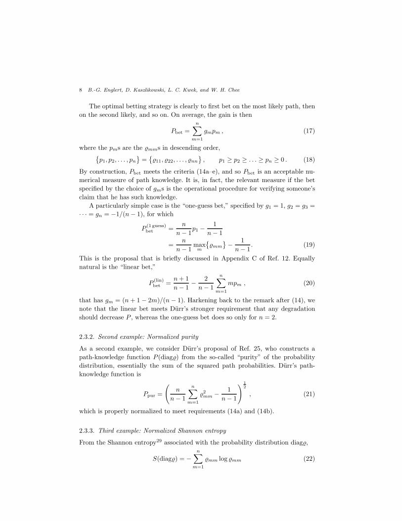
A particularly simple case is the “one-guess bet,” specified by g1 = 1, g2 = g3 =

· · · = gn = −1/(n− 1), for which

P(1 guess)bet =

n

n − 1p1 −

1

n − 1

=n

n − 1max

m

{

mm

}

− 1

n − 1. (19)

This is the proposal that is briefly discussed in Appendix C of Ref. 12. Equally

natural is the “linear bet,”

P(lin)bet =

n + 1

n − 1− 2

n − 1

n∑

m=1

mpm , (20)

that has gm = (n + 1 − 2m)/(n − 1). Harkening back to the remark after (14), we

note that the linear bet meets Durr’s stronger requirement that any degradation

should decrease P , whereas the one-guess bet does so only for n = 2.

2.3.2. Second example: Normalized purity

As a second example, we consider Durr’s proposal of Ref. 25, who constructs a

path-knowledge function P (diag) from the so-called “purity” of the probability

distribution, essentially the sum of the squared path probabilities. Durr’s path-

knowledge function is

Ppur =

(

n

n − 1

n∑

m=1

2mm − 1

n − 1

)12

, (21)

which is properly normalized to meet requirements (14a) and (14b).

2.3.3. Third example: Normalized Shannon entropy

From the Shannon entropy29 associated with the probability distribution diag,

S(diag) = −n∑

m=1

mm log mm (22)


one can construct yet another path-knowledge function. This approach was regarded

as the natural one by the authors of Refs. 6 and 9 in the context of two-path

interferometers, but was found less appealing for n-path interferometers by the

authors of Refs. 12 and 25.

Upon proper normalization to meet requirements (14a) and (14b), the entropic

measure of path knowledge is given by

Pent =1

log n

n∑

m=1

mm log(nmm) . (23)

Whereas the binary logarithm is usually understood in (22), it does not matter

which base value is chosen in (23).

2.3.4. Fourth example: Renyi-type measures

It is worth mentioning that, as a generalization of both the purity measure in (21)

and the entropic measure in (23), one could employ the Renyi-type measures that

are defined by

P(λ)Ren =

(

nλ

nλ − n

n∑

m=1

λmm − n

nλ − n

)1λ

(24)

where λ is a positive parameter.e We recover the purity measure for λ = 2 and the

entropic measure in the limit λ → 1,

P(2)Ren = Ppur , P

(1)Ren ≡ P

(λ→1)Ren = Pent , (25)

and intermediate λ values interpolate between Ppur and Pent.

There are also the limits λ → ∞ and λ → 0, both of which are peculiar. We

have

P(∞)Ren ≡ P

(λ→∞)Ren =

{

p1 if np1 > 1 ,

0 if np1 = 1 ,(26)

for λ → ∞, and

P(0)Ren ≡ P

(λ→0)Ren =

{

1 if p1 = 1 ,

0 if p1 < 1 ,(27)

for λ → 0. For both, the value of p1 = maxm

{mm} matters solely, which makes

P(∞)Ren , and to a much lesser extent also P

(0)Ren, somewhat similar to P

(1 guess)bet .

We are not examining these Renyi-type measures in the situations of n = 2 and

n = 3 that are dealt with in Secs. 3 and 4, but will offer a few comments on the

limiting measures P(∞)Ren and P

(0)Ren for arbitrary n values in Sec. 6.

eThe symbol p is usually used to denote the parameter in the standard definition of the family ofRenyi entropies, but we switch to λ in order to avoid confusion with the probabilities p1, . . . , pn.Further we note that we find it convenient to not take the logarithm of the sum in (24), whichwould be yet another option.


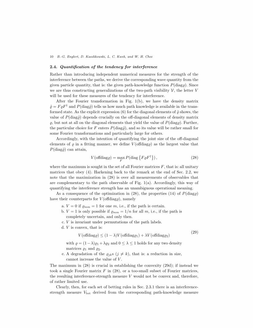
2.4. Quantification of the tendency for interference

Rather than introducing independent numerical measures for the strength of the

interference between the paths, we derive the corresponding wave quantity from the

given particle quantity, that is: the given path-knowledge function P (diag). Since

we are thus constructing generalizations of the two-path visibility V , the letter V

will be used for these measures of the tendency for interference.

After the Fourier transformation in Fig. 1(b), we have the density matrix

˜ = FF † and P (diag ˜) tells us how much path knowledge is available in the trans-

formed state. As the explicit expression (6) for the diagonal elements of ˜ shows, the

value of P (diag˜) depends crucially on the off-diagonal elements of density matrix

, but not at all on the diagonal elements that yield the value of P (diag). Further,

the particular choice for F enters P (diag˜), and so its value will be rather small for

some Fourier transformations and particularly large for others.

Accordingly, with the intention of quantifying the joint size of the off-diagonal

elements of in a fitting manner, we define V (offdiag) as the largest value that

P (diag˜) can attain,

V (offdiag) = maxF

P (diag{

FF †}) , (28)

where the maximum is sought in the set of all Fourier matrices F , that is: all unitary

matrices that obey (4). Harkening back to the remark at the end of Sec. 2.2, we

note that the maximization in (28) is over all measurements of observables that

are complementary to the path observable of Fig. 1(a). Accordingly, this way of

quantifying the interference strength has an unambiguous operational meaning.

As a consequence of the optimization in (28), the properties (14) of P (diag)

have their counterparts for V (offdiag), namely

a. V = 0 if mm = 1 for one m, i.e., if the path is certain.

b. V = 1 is only possible if mm = 1/n for all m, i.e., if the path is

completely uncertain, and only then.

c. V is invariant under permutations of the path labels.

d. V is convex, that is:

V (offdiag) ≤ (1 − λ)V (offdiag1) + λV (offdiag2)

with = (1−λ)1 +λ2 and 0 ≤ λ ≤ 1 holds for any two density

matrices 1 and 2.

e. A degradation of the jks (j 6= k), that is: a reduction in size,

cannot increase the value of V .

(29)

The maximum in (28) is crucial in establishing the convexity (29d); if instead we

took a single Fourier matrix F in (28), or a too-small subset of Fourier matrices,

the resulting interference-strength measure V would not be convex and, therefore,

of rather limited use.

Clearly, then, for each set of betting rules in Sec. 2.3.1 there is an interference-

strength measure Vbet derived from the corresponding path-knowledge measure


Pbet. In particular, we have V(1 guess)bet and V

(lin)bet paired with P

(1 guess)bet of (20) and

P(lin)bet of (21), respectively. And likewise, we have Vpur associated with Durr’s Ppur

of Sec. 2.3.2, and also an entropic Vent that goes with Pent of Sec. 2.3.3.

Each P, V pair can be used to study the compromises intermediate between the

extreme situations of “particle aspect only” (P = 1 and V = 0) and “wave aspect

only” (V = 1 and P = 0). Qualitatively, the same picture emerges for all P, V

pairs: Owing to the complementarity of the particle and wave modes of operation

(recall the remark at the end of Sec. 2.1), the two aspects are mutually exclusive

— if P = 1, then surely V = 0, and vice versa. In a P, V diagram, the extremal

points (P, V ) = (1, 0) and (P, V ) = (0, 1) are connected by a (curved) line, which

together with the straight lines to (P, V ) = (0, 0) encloses the area of all possible

pairs of P, V values. The shape of the line from (P, V ) = (1, 0) to (P, V ) = (0, 1)

and other quantitative details depend on the specific choice for the path-knowledge

function P (diag) and the induced interference-strength measure V (offdiag).

3. Two-path interferometers: Qubits

In Sec. 2, we have emphasized consistently, and somewhat pedantically, that the

various path-knowledge functions P (diag) involve only the diagonal elements of

, and the corresponding interference-strength measures V (offdiag) only the off-

diagonal elements. But from now on we shall simplify the notation and just write

P () and V ().

For a first illustration, and to make contact with familiar notions, we now con-

sider the particularly simple situation of two-path interferometers. Then, the in-

terfering object constitutes a binary quantum alternative, or qubit.f The familiar

expressions for the predictability P and the visibility V ,

P =∣

∣11 − 22

∣

∣ , V = 2∣

∣12

∣

∣ , (30)

are quite simply related to the elements of the 2 × 2 density matrix,

bit =

(

11 12

21 22

)

, (31)

and the basic inequality (1) is an immediate consequence of the normalization of

bit to unit trace (11 + 22 = 1) and its positivity (1221 ≤ 1122).

The n = 2 versions of the path-knowledge measures introduced in Sec. 2.3 are

simple monotonic functions of the predictability,

Pbet = Ppur = P ,

Pent =1

log 4

[

(1 + P) log(1 + P) + (1 − P) log(1 − P)]

, (32)

fThe alternative spelling q-bit is less popular. One of us, at least, thinks that this is regrettable,because “q-bit” perfectly fits the pattern of Dirac’s “q-numbers” and “c-numbers.”


0

0.2

0.4

0.6

0.8

1

0 0.2 0.4 0.6 0.8 1

P

V

a

b

Fig. 2. Possible values for the path-knowledge measure P and the interference-strength measureV in two-path interferometers. Curve a is the quarter-circle border line for (P, V ) = (Pbet, Vbet)and (P, V ) = (Ppur, Vpur), curve b is the border line for (P, V ) = (Pent, Vent). Pure-state valuesare on the respective border curves, mixed-state values are inside the area with corners at (P, V ) =(0, 0), (P, V ) = (1, 0), and (P, V ) = (0, 1). The shaded rectangle has the top-right corner on curveb; see text.

and the implied interference-strength measures of Sec. 2.4 are the same functions

of the visibility,

Vbet = Vpur = V ,

Vent =1

log 4

[

(1 + V) log(1 + V) + (1 − V) log(1 − V)]

. (33)

For each of these P, V pairs, pure states maximize the value of P for given V , and

the value of V for given P . This observation is an immediate consequence of (1),

where the equal sign applies for pure states.

To trace the border curve that connects (P, V ) = (1, 0) with (P, V ) = (0, 1) it

is quite sufficient to consider the projector matrices

bit,pure =

(

cosϑ

sinϑ

)

(

cosϑ, sinϑ)

with 0 ≤ ϑ ≤ 1

4π (34)

because any other pure-state density matrix differs from one of these bit,pures at

most by a permutation and a phase transformation, which are irrelevant in the

present context. For both the ‘bet’ pair and the ‘pur’ pair, the border curve is the

quarter circle labeled a in Fig. 2. For the ‘ent’ pair, the border is drawn by the

concave curve b, which appears to be at odds with the convexity of Pent and Vent

but in fact is not.


To justify this assertion we consider the qubit in an arbitrary mixed state, so

that

1122 > 0 and 12 = ε√

1122 with |ε| < 1 (35)

in (31). Now write ε = |ε|eiα and define λ = 12 (1 + |ε|). Then

bit = λ

(

11 eiα√1122

e−iα√1122 22

)

+ (1 − λ)

(

11 −eiα√1122

−e−iα√1122 22

)

≡ λ(1)bit + (1 − λ)

(2)bit . (36)

The two pure-state density matrices thus introduced, (1)bit and

(2)bit , have the same

predictability and visibility, namely P =∣

∣11 − 22

∣

∣ and V = 2√

1122. Therefore,

they also have the same P, V pair of values, irrespective of whether we chose the

‘bet’ pair, or the ‘pur’ pair, or the ‘ent’ pair. The convexity of P () and V () then

implies

P (bit) ≤ P (1,2) , V (bit) ≤ V (1,2) , (37)

where P (1,2) and V (1,2) are the common values of (1)bit and

(2)bit . This says that,

in Fig. 2, the point(

P (bit), V (bit))

is inside the rectangle with 0 ≤ P ≤ P (1,2),

0 ≤ V ≤ V (1,2).g For an exemplary pair P (1,2), V (1,2) on curve b, this rectangle is

shaded in Fig. 2. Clearly, it is wholly inside the area bounded by the axes and

curve b.

4. Three-path interferometers: Qutrits

Somewhat more interesting than two-path interferometers are three-path interfer-

ometers, in which the interfering object is a ternary quantum alternative, or qutrit.h

Here we have a 3 × 3 density matrix

trit =

11 12 13

21 22 23

31 32 33

(38)

that is normalized to unit trace (11 + 22 + 33 = 1) and positive, so that the

restrictions

tr{

2trit

}

≤ 1 , det{

trit

}

≥ 0 (39)

apply. Since phase transformations,

jk → ei(ϕj − ϕk)jk , (40)

gActually we have P (bit) = P (1,2) so that point (P (bit), V (bit)) lies on the right border of therectangle, but this detail is not relevant for the argument.hFootnote f applies mutatis mutandis.


turn a given trit into an equivalent one, we can adjust the complex phases of the

off-diagonal elements such that

12 = |12| e13iθ , 23 = |23| e

13iθ , 31 = |31| e

13iθ , (41)

with a common phase factor exp(13 iθ) that, for the given off-diagonal elements, is

determined by the phase-invariant product

122331 =∣

∣122331

∣

∣eiθ . (42)

With the convention that θ = 0 if 122331 = 0 and −π < θ ≤ π otherwise, the

value of θ is unique.

For n = 3, there is essentially only one complex number in the set of Eq. (13),

namely z1 = z∗2 ≡ z, explicitly given by

z = q11 + q222 + 33 , (43)

where

q ≡ ei2π/3 =−1 + i

√3

2(44)

is the basic cubic root of unity, for which

q3 = 1 , q2 = q∗ = q−1 , 1 + q + q2 = 0 (45)

are noteworthy identities. One can regard z as the average of q, q2, and q3 = 1 that

refers to the weights 11, 22, 33, respectively. Accordingly, when represented as

points in Gauss’s complex plane, the possible values of z are inside the equilateral

triangle that has its corners at 1, q, and q2.

The identities (45) are used, for example, when expressing the diagonal elements

of trit in terms of z,

11 = 13 (1 + q2z + qz∗)

22 = 13 (1 + qz + q2z∗)

33 = 13 (1 + z + z∗)

or kk = 13 + 2

3 Re(

q−kz)

. (46)

And, as a basic check of consistency, we note that tr {trit} = 1 is immediate.

Similarly, the diagonal elements ˜mm of the Fourier transformed density matrix

˜trit = FtritF† can be expressed in terms of the corresponding complex number

Z = eiϕ112e−iϕ2 + eiϕ223e

−iϕ3 + eiϕ331e−iϕ1 , (47)

where the phases ϕj are those of (5) and (7). Explicitly, we have

˜mm = 13 + 2

3 Re(

q−mZ)

(48)

as the analog of (46).


4.1. Pure qutrit states

The generic form of the density matrix for a pure qutrit state is

trit,pure =

p1√

p1p2√

p1p3√p2p1 p2

√p2p3√

p3p1√

p3p2 p3

=

√p1√p2√p3

(√p1,

√p2,

√p3

)

(49)

with p1 ≥ p2 ≥ p3 ≥ 0 by convention and p1 + p2 + p3 = 1 by normalization. There

are four families of pure states that are of particular importance, characterized by

Family Ia: p2 = p3 ;

Family Ib: (p1 − p3)2 + 3p2 = 1 ;

Family II: p1 = p2 ;

Family III: p3 = 0 .

(50)

Families Ia and Ib have the states of full path knowledge (p1 = 1, p2 = p3 = 0) and

of full interference strength (p1 = p2 = p3 = 13 ) as limiting cases. The latter is also

a member of Family II, whereas the former is in Family III. The respective other

limit of p1 = p2 = 12 , p3 = 0 is a common member of Families II and III. These

matters are summarized by the schematic diagram

.

...............................................

.............................................

............................................

..........................................

..

..

..

...................................

..

..

..

..

..

..

..

..

..

..

..

..

..

..

..

..

..

..

..

..

.

..

..

..

..

..

..

..

..

..

..

..

..

..

..

..

..

..

..

..

..

..

..

..

..

..

..

..

..

..

..

..

..

..

..

..

..

..

..

..

..

..

..

..

..

..

..

..

..

..

..

..

..

..

..

..

..

..

..

..

..

..

..

..

..

..

.

..

..

..

..

..

..

..

..

..

..

..

..

..

..

..

..

..

..

..

..

..

..

..

.

.

..

..

..

..

..

..

..

..

..

..

..

..

..

..

..

..

..

..

..

..

..

..

..

..

..

..

..

..

..

..

..

..

..

..

..

..

..

..

..

..

..

..

..

..

..

..

..

..

..

..

.

..

..

..

..

..

..

..

..

..

..

..

..

..

..

.

..

..

..

..

..

..

..

..

..

..

..

..

..

..

..

..

..

..

..

..

..

..

..

..

..

..

..

..

..

..

..

..

..

..

..

.

..

..

..

..

..

..

..

..

..

.

..

..

..

..

..

..

..

..

..

..

..

..

..

..

..

.

....................................

....................................

...................................

...................................

..................................

..

..

.............................

��✠

[p1, p2, p3] = [1, 0, 0]P = 1 , V = 0

��✠

[p1, p2, p3] = [13, 1

3, 1

3]

P = 0 , V = 1

��✒[p1, p2, p3] = [1

2, 1

2, 0]

P < 1 , V < 1

Ia or IbII

III

(51)

which shows how the families (50) interpolate between the particular limiting pure

states.

In Fig. 3, the families of (50) trace out the borders in the P, V diagram within

which the P, V values of all pure qutrit states are located. Despite the obvious

differences, all four plots have certain basic features in common: there is a smooth

outer border, and the inner border consists of two smooth pieces with a cusp where

they are joined. Note in particular that, in marked contrast to the two-path case,

not all pure states give an optimal compromise between P and V , only the ones on

the outer border achieve this.

The cusp for the pure state with p1 = p2 = 12 , p3 = 0, the common state of


0

0.2

0.4

0.6

0.8

1

0 0.2 0.4 0.6 0.8 1P

V

(a)

0

0.2

0.4

0.6

0.8

1

0 0.2 0.4 0.6 0.8 1P

V

(b)

0

0.2

0.4

0.6

0.8

1

0 0.2 0.4 0.6 0.8 1P

V

(c)

0

0.2

0.4

0.6

0.8

1

0 0.2 0.4 0.6 0.8 1P

V

(d)

Fig. 3. The P, V values of all pure qutrit states are located in the shaded areas or on the solidlines enclosing them. The four plots refer to quantifying path knowledge (a) by the one-guess bet,(b) by the linear bet, (c) by the purity measure, and (d) by the entropic measure. In all cases, theinner borders are traced out by families II and III of (51), whereas family Ia resides on the outerborder for (a), (c), and (d) but not for the linear-bet case (b), for which family Ib makes up theouter border.

families II and III, is at

(P, V ) =

(14 , 1

2 ) for the one-guess bet of Fig. 3a,

(12 , 1√

3) for the linear-guess bet of Fig. 3b,

(12 , 1

2 ) for the purity measure of Fig. 3c,

(1 − log3 2, 13 log3 2) for the entropic measure of Fig. 3d.

(52)

The outer border is formed by family Ia, except for the linear-guess bet of Fig. 3b

where the state of family Ib reside on the outer border. We now proceed to take a

look at the various measures for the path knowledge and the implied measures for

the interference strength in order to justify these remarks.


4.1.1. One-guess bet

The path knowledge associated with the one-guess bet, see (19), is

P(1 guess)bet = 3

2p1 − 12 , (53)

and the corresponding measure for the interference strength is

V(1 guess)bet =

√p1p2 +

√p2p3 +

√p3p1 , (54)

as the maximization required by (28) is an optimization of the phase factors in

(47) which is easily carried out. We find the borders by maximizing and minimizing

V(1 guess)bet for a given value of P

(1 guess)bet , that is:

p1 given; p2 in the range 12 (1 − p1) ≤ p2 ≤ min{p1, 1 − p1};

p3 = 1 − p1 − p2; then

∂

∂p2V

(1 guess)bet = − (

√p2 −

√p3)(

√p1 +

√p2 +

√p3)

2√

p2p3≤ 0 ,

so that V(1 guess)bet is largest when p2 is smallest, and smallest

when p2 is largest.

(55)

Therefore, we have p2 = p3 on the outer border (family Ia), and p1 = p2 on the

inner border if p1 ≤ 12 (family II) as well as p2 = 1 − p1 on the inner border if

p1 ≥ 12 (family III). In geometrical terms, the outer border is (an arc of) the ellipse

2(P + V − 12 )2 + (P − V )2 = 3

2 , (56)

with the center at P = V = 14 , the major axis of length

√3 on the line V + P = 1

2

and the minor axis of length√

3/2 on the line V = P .

4.1.2. Linear bet

According to (20), we have the path knowledge

P(lin)bet = p1 − p3 (57)

for the linear betting strategy. Several steps are needed to find the corresponding

V(lin)bet . First, we recall the remark after Eq. (9) and set ϕ2 = 0 in

Z =√

p1p2 eiϕ1 +√

p2p3 e−iϕ3 +√

p3p1 ei(ϕ3 − ϕ1) . (58)

Second, we note that the replacements ϕ1 → ϕ1 + 2π3 , ϕ3 → ϕ3 − 2π

3 amount to

Z → qZ and thus permute the ˜mms of (48) cyclically. Therefore, it is permissible

to assume that∣

∣ ˜11 − ˜22

∣

∣ is the difference of the largest and the smallest of the

˜mms, so that

V(lin)bet =

2√3

maxϕ1,ϕ3

∣

∣Im(Z)∣

∣

=2√3

maxϕ1,ϕ3

{√p1p2 sin ϕ1 −

√p2p3 sin ϕ3 +

√p3p1 sin(ϕ3 − ϕ1)

}

. (59)


Third, we perform the required maximization over ϕ1 and ϕ3 and arrive at

V(lin)bet =

2√3

√

p1p2 + p2p3 + p3p1 + 2y + 3y2

where y ≥ 0 solves 2y3 + y2 = p1p2p3. (60)

If an explicit expression is needed for y, then

y =cos(3ϑ)

6 cosϑwith cos(3ϑ) =

√

27p1p2p3 (61)

is perhaps the most convenient.

We now search for the largest value of V(lin)bet for a given value of P

(lin)bet , that is

the difference P ≡ p1 − p3 is fixed. The permissible values of p2 are then in the

range

13 (1 − P ) ≤ p2 ≤

{

13 (1 + P ) for P ≤ 1

2 ,

1 − P for P ≥ 12 .

(62)

If p2 equals its lower bound, the state is in family Ia; at the upper bounds we have

family II or III, respectively.

We note that dp1 = dp3 = − 12dp2, with the consequence

d

dp2V

(lin)bet

2=

1

3y

[

(1 − 3p2)(1 − p2 + 2y) − P 2]

. (63)

At the bounds on p2 in (62) we thus have

d

dp2V

(lin)bet > 0 at the lower bound,

andd

dp2V

(lin)bet < 0 at the upper bounds. (64)

Therefore, V(lin)bet has local minima for families Ia, II, and III. The smaller value is

always obtained for the upper bounds in (62), as one can verify after first observing

that

lower bound: p1 = 13 (1 + 2P ) , p2 = p3 = 1

3 (1 − P ) ,

2y2 + p1y = p1p3 ;

upper bound for P ≤ 12 : p1 = p2 = 1

3 (1 + P ) , p3 = 13 (1 − 2P ) ,

2y2 + p3y = p1p3 ;

upper bound for P ≥ 12 : p1 = P , p2 = 1 − P , p3 = 0 , y = 0 ;

(65)

so that families II and III trace out the inner borders, indeed.

Further, Eq. (63) implies that V(lin)bet is maximal at the intermediate p2 value

that obeys

(1 − 3p2)(1 − p2 + 2y) = P 2 (66)


with y from (60). Therefore, the pure state with

p1 = 16 (1 + P )(2 + P ) , p2 = 1

3 (1 − P 2) ,

p3 = 16 (1 − P )(2 − P ) , y = 1

6 (1 − P 2) , (67)

maximizes V(lin)bet for given P = P

(lin)bet . Indeed, the outer border of Fig. 3b is traced

by family Ib of (50). And since V(lin)bet =

√1 − P 2 for the pure states specified by

(67), the outer border is the quarter circle

P 2 + V 2 = 1 . (68)

4.1.3. Purity

It is a matter of inspection to verify that the path-knowledge function of Sec. 2.3.2

is given by the modulus of z,

Ppur = |z| . (69)

It follows that the induced interference-strength measure is

Vpur = maxϕj

{

|Z|}

= |12| + |23| + |31| , (70)

because the maximal value of |Z| obtains when the phases ϕj are just the ones that

exhibit the common phase factor exp(13 iθ) of (41). These equations apply to pure

or mixed states.

We note that, although Ppur is Durr’s path knowledge function of Ref. 25, the

corresponding interference strength Vpur of (70) is not the one suggested by Durr,

which is

V pur =

√

3(

|12|2+ |23|

2+ |31|

2). (71)

Therefore, Durr’s pair Ppur, V pur does not fit into the general strategy of Sec. 2.

Rather than linking V to P by (28), his choice is such that

P 2 + V 2 = 32 tr{

2trit

}

− 12 ≤ 1 (72)

by construction. The equal sign holds for all pure states, as it does in Eq. (1).

For pure states, Eqs. (69) and (70) give

Ppur =√

1 − 3(p1p2 + p2p3 + p3p1) ,

Vpur =√

p1p2 +√

p2p3 +√

p3p1 . (73)

We note the coincidence that Ppur = P(1 guess)bet and Vpur = V

(1 guess)bet on the outer

border, traced out by family Ia, so that the outer border for the purity measures is

also the ellipse (56) of the one-guess bet.


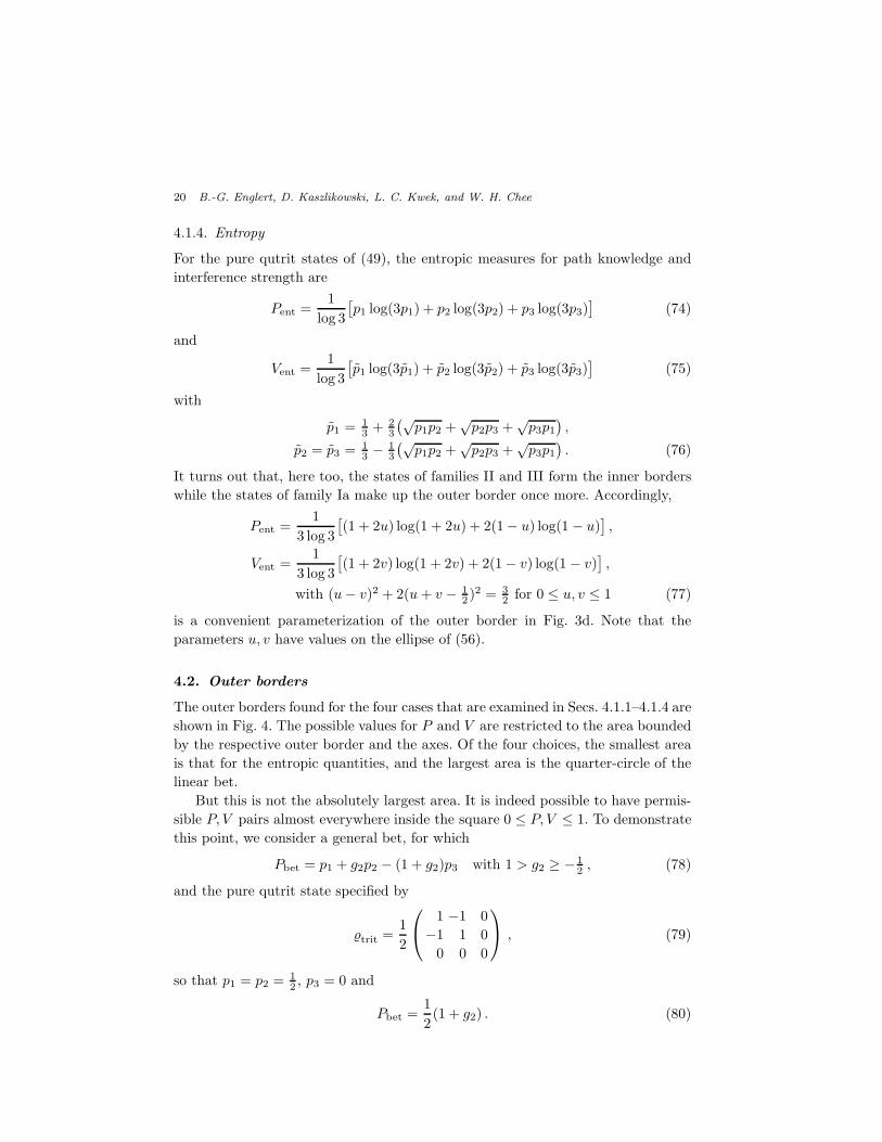
4.1.4. Entropy

For the pure qutrit states of (49), the entropic measures for path knowledge and

interference strength are

Pent =1

log 3

[

p1 log(3p1) + p2 log(3p2) + p3 log(3p3)]

(74)

and

Vent =1

log 3

[

p1 log(3p1) + p2 log(3p2) + p3 log(3p3)]

(75)

with

p1 = 13 + 2

3

(√p1p2 +

√p2p3 +

√p3p1

)

,

p2 = p3 = 13 − 1

3

(√p1p2 +

√p2p3 +

√p3p1

)

. (76)

It turns out that, here too, the states of families II and III form the inner borders

while the states of family Ia make up the outer border once more. Accordingly,

Pent =1

3 log 3

[

(1 + 2u) log(1 + 2u) + 2(1 − u) log(1 − u)]

,

Vent =1

3 log 3

[

(1 + 2v) log(1 + 2v) + 2(1 − v) log(1 − v)]

,

with (u − v)2 + 2(u + v − 12 )2 = 3

2 for 0 ≤ u, v ≤ 1 (77)

is a convenient parameterization of the outer border in Fig. 3d. Note that the

parameters u, v have values on the ellipse of (56).

4.2. Outer borders

The outer borders found for the four cases that are examined in Secs. 4.1.1–4.1.4 are

shown in Fig. 4. The possible values for P and V are restricted to the area bounded

by the respective outer border and the axes. Of the four choices, the smallest area

is that for the entropic quantities, and the largest area is the quarter-circle of the

linear bet.

But this is not the absolutely largest area. It is indeed possible to have permis-

sible P, V pairs almost everywhere inside the square 0 ≤ P, V ≤ 1. To demonstrate

this point, we consider a general bet, for which

Pbet = p1 + g2p2 − (1 + g2)p3 with 1 > g2 ≥ − 12 , (78)

and the pure qutrit state specified by

trit =1

2

1 −1 0

−1 1 0

0 0 0

, (79)

so that p1 = p2 = 12 , p3 = 0 and

Pbet =1

2(1 + g2) . (80)


0

0.2

0.4

0.6

0.8

1

0 0.2 0.4 0.6 0.8 1

P

V

b

a&c

d

Fig. 4. The outer borders of the shaded areas in Fig. 3. For Figs. 3a and 3c we have curve a&c,the ellipse of Eq. (56). Curve b is the circle of Eq. (68), the outer border in Fig. 3b. For theentropic measures of Fig. 3d, the P, V values of (77) are shown as curve d.

For either one of the two 3 × 3 Fourier matrices in (11) we have FtritF† = trit,

implying

1

2(1 + g2) ≤ Vbet < 1 . (81)

By now choosing g2 sufficiently close to, but less than, unity, we can push (Pbet, Vbet)

as close to the corner (P, V ) = (1, 1) as we wish. As a consequence of criterion (14a),

the limiting value g2 = 1 is not permitted in (16); if it were, it would realize a bet

on two of the three paths versus the third. In practice, however, a g2 value that

is rather close to 1 will implement such a 2-of-3 bet quite well, and then the two

dominating paths can interfere with almost full strength even when almost perfect

2-of-3 path knowledge is at hand.

For the pure qutrit states of (49) we have

Pbet → 1 − 3p3

and Vbet →{

1 if√

p1 ≤ √p2 +

√p3 ,

2(√

p1p2 −√

p2p3 +√

p3p1

)

if√

p1 ≥ √p2 +

√p3 ,

(82)

in the limit g2 → 1. Clearly, all states with p1 = p2, those of family II in (50), have

Vbet = 1 in this limit, so that the outer border is given by

max{P, V } = 1 , (83)

and the whole area of the square 0 ≤ P, V ≤ 1 is covered.


5. Four-path interferometers: Ququarts

In an interferometer with four paths, the interfering object is a quaternary quantum

alternative or ququart.i As a consequence of the parameter t in the 4 × 4 Fourier

matrix (12) and the nonequivalence of column permutations and row permutations,

the analysis of four-path interferometers is much more involved than that of inter-

ferometers with two or three paths and has not been carried out in full as yet. We

shall therefore be brief and only discuss two issues: Two conjectures, one disproven

by a counter example and the other undecided, and a recent analysis of a four-path

interferometer with the tools of two-path interferometry.

5.1. Linear bet: One conjecture rejected, another proposed

Whereas the border lines in the P, V -diagram are different, as a rule, for two-path

and three-path interferometers, it is remarkable that we have the same quarter-

circle border for the linear bet in Figs. 2 and 4. It is tempting to conjecture that

the linear bet values of (P, V ) are in the quarter-circle area P 2 + V 2 ≤ 1 also in

the case of four-path interferometers, or perhaps even quite generally for n-path

interferometers. This conjecture is, however, false as can be demonstrated by the

following counter example.32

Consider the pure-case 4 × 4 density matrix

=

√p4√p3√p2√p1

(√p4,

√p3,

√p2,

√p1

)

(84)

with the path probabilities

p1 =1

10G−4 , p2 =

1

10G−2 , p3 =

1

10G2 , p4 =

1

10G4 , (85)

where G = 12 (√

5 − 1) is the golden ratio. The t = 0 Fourier matrix (12) yields

˜ = , so that V(lin)bet () ≥ P

(lin)bet (˜) = P

(lin)bet () =

√

5/9, and

P(lin)bet

2+ V

(lin)bet

2≥ 10

9> 1 (86)

for this .

There is numerical evidence, but no clear-cut demonstration of the case as yet,

that the linear-bet border is traced out by pure states with density matrices of the

form (84) with√

p1/p2 =√

p3/p4 = eϑ ,√

p3/p1 =√

p4/p2 = tanhθ

2where 4 sinh ϑ sinh θ = 1 , (87)

iWe follow the practice of recent publication, such as Ref. 30, although ququad could be preferable,inasmuch as 1 quad = 2bits according to the Hackers’ Dictionary,31 which offers tayste as a seriousalternative to quad and crumb as a silly alternative but does not mention quart. Footnote f appliesmutatis mutandis.


0

0.2

0.4

0.6

0.8

1

0 0.2 0.4 0.6 0.8 1

P

V

a

b

Fig. 5. Possible values for the path-knowledge measure P and the interference-strength measure

V in four-path interferometers. Curve a is the conjectured border line for (P, V ) = (P(lin)bet , V

(lin)bet )

that is traced out by (89), and curve b is the quarter circle P 2 + V 2 = 1 .

and the optimal Fourier transform being the t = 1 version of (12). Then we have

√

p1/p2 =√

p3/p4 = eθ ,√

p3/p1 =√

p4/p2 = tanhϑ

2, (88)

which are reciprocal to the relations in (87), and

P(lin)bet =

1

3tanhϑ +

2

3sech θ , V

(lin)bet =

1

3tanh θ +

2

3sech ϑ (89)

parameterize the thus conjectured border line. Figure 5 shows that, except for

(P, V ) = (1, 0) and (P, V ) = (0, 1), all values of (89) have P(lin)bet

2+ V

(lin)bet

2> 1. The

values of (85) and (86) obtain for sinhϑ = sinh θ = 12 .

5.2. 4 6= 2 × 2

In a recent series of papers, there is a claim that one can violate the duality rela-

tion (1), thereby “cheating on complementarity” in this manner; see Ref. 33, for

instance. Of course, Bohr’s Principle of Complementarity,j the fundamental prin-

ciple of quantum kinematics, remains untouched: in fact, the authors of Ref. 33

are relying on it in their analysis, as all arguments do that invoke the quantum

formalism.

jSee Ref. 34 for a textbook discussion.


More importantly, the thought experiment in question — a Mach-Zehnder (MZ)

set-up traversed by a qubit, so that the spatial binary alternative of the MZ ge-

ometry and the internal qubit together make up a ququart — is a four-path in-

terferometerk to which the two-path relation (1) does not apply. When applying it

nevertheless, by letting path knowledge refer solely to the arms of the MZ set-up,

the actual paths of the four-path interferometer are grouped into two pairs, and we

have a 2-of-4 bet, similar to the 2-of-3 bet discussed in Sec. 4.2.

The situation is then that of a limiting four-path bet with g1 = 1, g4 = −1, and

1 > g2 = −g3 → 1, and it is easy to have both P and V close to unity. But this has

no bearing on (1) or any other relation for two-path interferometers, and poses no

challenge to complementarity.

An analysis of the ququart MZ set-up as a four-path interferometer with the

methodology introduced in Sec. 2 would be of great interest. If the four paths are

implemented by having polarized photons in the two arms of a MZ interferometer,

the particle mode and the wave mode of Fig. 1 can be realized by known and rather

simple tools.35

6. n-path interferometers: Qunits

In a multi-path interferometer with n paths, the generic situation of Fig. 1, the

interfering object is a n-fold quantum alternative, or qunit.l Little is known about

the possible (P, V ) values for qunits. We can only offer some observations about

path knowledge measures that involve solely p1 and put on record an unproven

conjecture about the pair (Pent, Vent) of entropic measures that is suggested by a

pattern observed for qubits and qutrits, and by some numerical evidence.

6.1. Entropic measures: A conjecture

The conjecture is this: The border lines for the entropic measures for path knowledge

and interference strength are traced out by the pure states whose n × n density

matrices are of the form

=

√p2√p2

...√p2√p1

(√p2,

√p2, . . . ,

√p2,

√p1

)

with p1 + (n − 1)p2 = 1 , (90)

kIn the MZ set-up of Ref. 33 there are fixed relations between the phases φ1, . . . , φ4 of the fourpath amplitudes, so that the full flexibility needed in (28) would require a modification of theset-up.lOther authors prefer to speak of qudits, having d-dimensional Hilbert subspaces in mind. Heretoo, footnote f applies mutatis mutandis.


(a)

(b)

0

0.2

0.4

0.6

0.8

1

0 0.2 0.4 0.6 0.8 1

P

V

ab

cd

0.394

0.396

0.398

0.4

2 6 10 14 18n

P = V

Fig. 6. Conjectured border lines for the entropic measures for path knowledge and interferencestrength in multi-path interferometers. The top plot (a) shows the border lines associated with(90) and (91), whereby curve a is for n = 2, curve b for n = 10, curve c for n = 107, and curve d

for n → ∞. — The bottom plot (b) shows the symmetric P = V values for n = 2, 3, . . . , 20 andconfirms that the smallest value is found for n = 10.

and the optimal Fourier matrix is the standard one of (5)—(7) with ϕj = 0. Then

˜ has the same form with p1 and p2 replaced by

p1 =1

n

(√p1 + (n − 1)

√p2

)2and p2 =

1

n

(√p1 −

√p2

)2, (91)

respectively. The identities

np1 + np1 − 2√

np1p1 = n − 1 , np2 + np2 + 2√

np2p2 = 1 (92)

exhibit the reciprocal nature of the mappings (p1, p2) ↔ (p1, p2).

Thus surmising that these pure states are on the border of the (Pent, Vent) values

in the P, V -diagram, we get the border lines of Fig. 6(a). For moderate n values,

the border lines are very similar to the n = 2 line in Fig. 2 and the n = 3 line in

Fig. 4, whereas we get the straight line Pent + Vent = 1 in the limit of n → ∞.


The conjectured border lines of Fig. 6(a) have the remarkable feature that the

area of permissible (Pent, Vent) values decreases from n = 2 to n = 10 and then in-

creases.m This is illustrated by the plot in Fig. 6(b) which shows, for n = 2, 3, . . . , 20,

the symmetric values

Pent = Vent = logn

√n

2+

1√n

logn(√

n + 1) (93)

that one gets for

p1 = p1 =

√n + 1

2√

n, p2 = p2 =

1

2√

n(√

n + 1), (94)

with the right-hand side of (93) equal to 0.394845, 0.394820, and 0.394827 for n = 9,

10, and 11, respectively. We leave it at that.

6.2. Measures based solely on p1 = maxm

{mm}

In (19), (26), and (26) we encounter path knowledge measures that involve only

p1 = maxm

{mm}: the measure of the one-bet guess P(1 guess)bet and the extreme limits

P(∞)Ren and P

(0)Ren of the Renyi-type measures. For these, it is clear that the pure states

of (90)–(92) maximize V for given P , and P for given V .

Another way of writing the first identity in (92),

n(

p1 + p1 − 1)2

+n

n − 1

(

p1 − p1)2 = 1 , (95)

gives us the border lines for P(1 guess)bet and P

(∞)Ren . In the case of the one-guess bet,

we have P = (np1 − 1)/(n − 1) and V = (np1 − 1)/(n − 1), and it follows that the

border line is an arc of the ellipse

(n − 1)2

n

(

P + V − n − 2

n − 1

)2

+n − 1

n

(

P − V)2

= 1 . (96)

As it should, this is the ellipse of (56) for n = 3, and the circle P 2 + V 2 = 1 for

n = 2. The ellipse of (96) is centered at P = V = (n − 2)/(2n − 2); its major axis

of length√

2n/(n− 1) is on the line V + P = (n − 2)/(n − 1), and the minor axis

of length√

2n/(n − 1) is on the line P = V .

In case of the Renyi-type measure for λ → ∞, it is P = p1 and V = p1 except

when p1 = 1, p1 = 1/n or p1 = 1/n, p1 = 1, and we have the arc with P > 1/n and

V > 1/n of the ellipse

n(

P + V − 1)2

+n

n − 1

(

P − V )2 = 1 (97)

as part of the border line. The straight lines with P ≤ 1/n and V = 1 or P = 1

and V ≤ 1/n complete the border line, but the points on these straight segments

are not permitted, except for the corners at (P, V ) = (1, 0) and (P, V ) = (0, 1).

mWe resist the strong temptation to suggest that this particular role that n = 10 plays in thecontext of wave-particle duality explains why humans have ten fingers.


In the limit n → ∞, the straight line P + V = 1 is the border for

(P(1 guess)bet , V

(1 guess)bet ) and (P

(∞)Ren , V

(∞)Ren ). The same line is conjectured above for

(Pent, Vent) for n → ∞.

By contrast, matters are quite simple in the λ → 0 limit of the Renyi-type

measures. All permissible values for (P(0)Ren, V

(0)Ren) have either P

(0)Ren = 0 or V

(0)Ren = 0.

7. Summary

We have presented a systematic way of quantifying path knowledge and interfer-

ence strength in multi-path interferometers. The quantitative measures for particle

aspects (path knowledge) and wave aspects (interference strength) have a clear

operational meaning and are naturally linked to each other. This systematic link,

which exploits general Fourier transformations, distinguishes our approach from

earlier attempts.

Since there is no unique procedure for assigning a single number to the

path knowledge when there are more than two paths, we have discussed sev-

eral self-suggesting definitions of the path-knowledge measure P and the induced

interference-strength measure V . As a consequence of wave-particle duality, P = 1

implies V = 0 and V = 1 implies P = 0 for all choices, but the range of values

allowed for the pair (P, V ) depends on the particular choice.

We have illustrated our approach with the familiar example of two-path inter-

ferometers and a thorough analysis of three-path interferometers, and have given

glimpses at four-path interferometers and general multi-path interferometers. This

sets the stage for further studies.

Perhaps the most important step to be taken now is an investigation the multi-

path analog of the transition from predictability to distinguishability in two-path

interferometers.13 We will report from this front in due course.

Acknowledgments

BGE is grateful for the hospitality extended to him by Christian Miniatura at the

Institut Nonlineaire de Nice in 2005 and 2007, where part of this work was car-

ried out. We acknowledge support by A*STAR Temasek Grant 012-104-0040 and

by NUS Grant R-144-000-179-112. Centre for Quantum Technologies is a Research

Centre of Excellence funded by Ministry of Education and National Research Foun-

dation of Singapore.

References

1. A. Einstein, Ann. Physik 17, 132 (1905); English translation in Ref. 36.2. N. Bohr, Die Naturwissenschaften 16, 245 (1928); English Version: Nature 121, 580

(1928); the latter is reprinted in Ref. 37.3. N. Bohr, “Discussions with Einstein on Epistemological Problems in Atomic Physics”

in Albert Einstein: Philosopher–Scientist, ed. P. A. Schilpp (Library of Living Philoso-phers, Evanston, 1949); reprinted in Ref. 37.


4. C. Held, Die Bohr-Einstein-Debatte (Schoeningh, Paderborn, 1998).5. B.-G. Englert and J. A. Bergou, Opt. Commun. 179, 337 (2000).6. W. K. Wootters and W. H. Zurek, Phys. Rev. D 19, 473 (1979).7. H. Rauch and J. Summhammer, Phys. Lett. A104, 44 (1984).8. R. Glauber, Ann. N. Y. Acad. Sci. 480, 336 (1986).9. P. Mittelstaedt, A. Prieur, and R. Schieder, Found. Phys. 17, 891 (1987).

10. D. M. Greenberger and A. Yasin, Phys. Lett. A128, 391 (1988).11. L. Mandel, Opt. Lett. 16, 1882 (1991).12. G. Jaeger, A. Shimony, and L. Vaidman, Phys. Rev. A 51, 54 (1995).13. B.-G. Englert, Phys. Rev. Lett. 77, 2154 (1996).14. B.-G. Englert, Z. Naturforsch. 54a, 11 (1999).15. J. Baldzuhn, E. Mohler, and W. Martienssen, Z. Phys. B77, 347 (1989).16. J. Baldzuhn and W. Martienssen, Z. Phys. B82, 309 (1991).17. P. D. D. Schwindt, P. G. Kwiat, and B.-G. Englert, Phys. Rev. A 60, 4285 (1999).18. P. G. Kwiat, P. D. D. Schwindt, and B.-G. Englert, “What does a quantum eraser

erase?” in Mysteries, Puzzles, and Paradoxes in Quantum Mechanics, ed. R. Bonifacio(CP461, The American Institute of Physics, 1999).

19. A. Trifonov, G. Bjork, J. Soderholm, and T. Tsegaye, Eur. Phys. J. D 18, 251 (2002).20. S. P. Walborn, M. O. Terra Cunha, S. Padua, and C. H. Monken, Phys. Rev. A 65,

033818 (2002).21. J. Summhammer, H. Rauch, and D. Tuppinger, Phys. Rev. A 36, 4447 (1987).22. S. Durr, T. Nonn, and G. Rempe, Nature 395, 33 (1998).23. S. Durr, T. Nonn, and G. Rempe, Phys. Rev. Lett. 81, 5705 (1998).24. M. Mei and M. Weitz, Phys. Rev. Lett. 86, 559 (2001).25. S. Durr, Phys. Rev. A 64, 042113 (2001).26. A. Luis, J. Phys. A: Math. Gen. 34, 8597 (2001).27. K. Zyczkowski and W. Tadej, http://chaos.if.uj.edu.pl/∼karol/hadamard/28. W. Tadej and K. Zyczkowski, Open Syst. Inf. Dyn. 13, 133 (2006).29. C. E. Shannon, Bell Sys. Tech. J. 27, 623 (1948).30. E. V. Moreva, G. A. Maslennikov, S. S. Straupe, and S. P. Kulik, Phys. Rev. Lett.

97, 023602 (2006).31. http://www.worldwideschool.org/library/books/tech/computers/

TheHackersDictionaryofComputerJargon/chap42.html32. W. H. Chee, Quantitative wave-particle duality in higher dimensions (unpublished

thesis, Singapore, 2005).33. G. Kurizki, N. Bar-Gill, J. Clausen, M. Kolar, and T. Opatrny, Quant. Inf. Processing

5, 463 (2006).34. B.-G. Englert, Lectures on Quantum Mechanics — Perturbed Evolution (World Sci-

entific, Singapore, 2006).35. B.-G. Englert, C. Kurtsiefer, and H. Weinfurter, Phys. Rev. A 63, 032303 (2001).36. D. ter Haar, The Old Quantum Theory (Pergamon Press, Oxford and New York,

1967).37. Quantum Theory and Measurement, eds. J. A. Wheeler and W. H. Zurek (Princeton

University Press, Princeton, 1983).

Wave-particle duality in multi-path interferometers: General concepts and three-path interferometers

Documents

Transcript of Wave-particle duality in multi-path interferometers: General concepts and three-path interferometers