Sheaves on abelian surfaces and strange duality

SHEAVES ON ABELIAN SURFACES AND STRANGE DUALITY

ALINA MARIAN AND DRAGOS OPREA

Abstract. We formulate three versions of a strange duality conjecture for sections ofthe Theta bundles on the moduli spaces of sheaves on abelian surfaces. As supportingevidence, we check the equality of dimensions on dual moduli spaces, answering aquestion raised by Gottsche-Nakajima-Yoshioka [GNY].

1. Introduction

Let (A,H) be a polarized abelian surface. In this paper, we consider the moduli spaces

of Gieseker H-semistable sheaves on A, and sections of the Theta line bundles defined

over them.

It will be convenient to bookkeep coherent sheaves E on A by their Mukai vectors,

setting

v(E) = r + c1(E) + χ(E)ω ∈ H2?(A),

where ω stands for the class of a point. As customary, we will equip the even cohomology

H2?(A) with the Mukai pairing. For any two vectors x = (x0, x2, x4) ∈ H2?(A) and

y = (y0, y2, y4) ∈ H2?(A), we set

〈x, y〉 = −∫Ax∨ ∪ y =

∫A

(x2y2 − x0y4 − x4y0) .

It follows that for any two sheaves E and F , we have

χ(E,F ) =

2∑i=0

(−1)i Exti(E,F ) = −〈v(E), v(F )〉.

For an arbitrary v ∈ H2?(A), let us write Mv for the moduli space of Gieseker H-

semistable sheaves E on A, with Mukai vector v. To keep things simple, we will make

the following assumption throughout:

Assumption 1. (i) The polarization H is generic i.e., it belongs to the complement

of a locally finite union of hyperplane walls in the ample cone of A;

(ii) The vector v is a primitive element of the lattice H2?(A,Z);

(iii) The vector v is positive i.e., one of the following is true:

– rank (v) > 0;1

2 ALINA MARIAN AND DRAGOS OPREA

– rank (v) = 0 and c1(v) is effective, χ(v) 6= 0, and 〈v, v〉 6= 0, 4.

The choice of generic polarization will play only a minor role in what follows, and as

such, we will supress it from the notation. Note that (i) and (ii) together imply that

Mv consists of stable sheaves only. Therefore, by [Muk3], Mv is a smooth manifold of

dimension 2dv + 2, with

(1) dv =1

2〈v, v〉.

The main characters of our story will be a collection of naturally defined Theta line

bundles on Mv. Consider the subgroup v⊥ inside the holomorphic K-theory of A gener-

ated by the sheaves F whose Mukai vectors w are orthogonal to v:

(2) χ(v ⊗ w) = −〈v∨, w〉 = 0.

There is a morphism

Θ : v⊥ → Pic(Mv), [F ]→ ΘF ,

constructed and studied by Li and Le Potier [Li] [LP] in the case of surfaces, and also

by Drezet-Narasimhan in the case of curves [DN]. The construction is easiest to explain

assuming that Mv is a fine moduli space, such that E is the universal sheaf on Mv ×A.

In this case, for a sheaf F with Mukai vector w, we set

(3) ΘF = det Rp!(E ⊗ q?F )−1,

where p and q are the two projections from Mv ×A. The orthogonality condition (2) is

used to obtain a well defined line bundle ΘF , even in the absence of universal structures,

by descent from the Quot scheme.

Note that even though the line bundle ΘF depends on the K-theory class of F , the

Chern class c1(ΘF ) depends only on the Mukai vector w. For simplicity of notation, in all

cohomological computations below, we will write Θw for any one of the line bundles ΘF

as above. The finer dependence of the line bundles ΘF on the sheaf F will be discussed

in more detail in Section 2.

Our goal in this paper is to compute the Euler characteristics of the line bundles Θw,

which can be interpreted as the K-theoretic Donaldson invariants of the abelian surface

A. We will provide a simple expression for these Euler characteristics, valid in any rank.

We will thus answer a question raised in [GNY], as part of a general study of the rank

two K-theoretic Donaldson invariants of surfaces.

SHEAVES ON ABELIAN SURFACES AND STRANGE DUALITY 3

To explain the results, let us first fix a reference line bundle Λ on A with c1(Λ) = c1(v).

Then, we have a well-defined determinant morphism

(4) α+Λ : Mv → A = Pic0(A), E → detE ⊗ Λ−1.

Its fiber over the origin is the moduli space M+v (Λ) of sheaves with fixed determinant Λ.

The choice of the determinant is unimportant for our arguments, and therefore we will

omit it from our notation when no confusion is likely to arise. We will show:

Theorem 1. For any vectors v and w satisfying Assumption 1, and such that χ(v⊗w) =

0, we have

(5) χ(M+v ,Θw) = χ(M+

w ,Θv) =1

2

c1(v ⊗ w)2

dv + dw

(dv + dwdv

).

There is yet another moduli space of interest to us, which is Fourier-Mukai ‘dual’ to

the one considered above. Letting P denote the normalized Poincare bundle on A× A,

the Fourier-Mukai transform is defined by

(6) RS(E) = Rp!(P ⊗ q?E) ∈ D(A),

where p, q are the two projections. With this understood, let us set

α−Λ : Mv → A, E → det RS(E)⊗ det RS(Λ)−1.

The fiber of the morphism α−Λ over the origin is denoted by M−v , and parametrizes sheaves

E with fixed determinant of the Fourier-Mukai transform. We will prove:

Theorem 2. For any vectors v and w as in Theorem 1, we have

(7) χ(M−v ,Θw) = χ(M−w ,Θv) =1

2

c1(v ⊗ w)2

dv + dw

(dv + dwdv

).

Here v and w denote the Fourier-Mukai transforms of the two vectors v and w.

Finally, we may consider the morphism

av = (α+Λ , α

−Λ) : Mv → A×A.

This is the Albanese map of the moduli space Mv, cf. [Y1]. Its fiber over the origin will

henceforth be denoted by Kv. We will show:

Theorem 3. Assume that the Neron-Severi group of A has rank 1. With the same

hypotheses as in Theorem 1, we have

(8) χ(Kv,Θw) = χ(Mw,Θv) =d2v

dv + dw

(dv + dwdv

).


The manifest symmetry of the formulas in Theorems 1, 2 and 3 matches first of all

that of their counterpart for the case of sheaves on a K3 surface. Indeed, the theta Euler

characteristics for the moduli space of sheaves on a K3 were shown to be [GNY][OG]

(9) χ(Mv,Θw) = χ(Mw,Θv) =

(dv + dw + 2

dv + 1

).

This symmetry further suggests a general strange duality for surfaces, reminiscent of

the case of moduli spaces of bundles on curves. There, the analogous invariance of the

Verlinde formula reflects a geometric isomorphism between generalized theta functions

with dual ranks and levels [B][MO1]. In the case of sheaves on an abelian or K3 surface,

it is tempting to assert, similarly, that whenever defined and nonzero, the morphisms

SD± : H0(M±v ,Θw)∨ → H0(M±w ,Θv)

are isomorphisms. The same considerations should apply to the companion morphism

SD : H0(Kv,Θw)∨ → H0(Mw,Θv).

In the above, for each of the three pairs of moduli spaces i.e., (M±v ,M±w) and (Kv,Mw),

the line bundle Θv stands for any one of the ΘE ’s, for E in the corresponding moduli

space of sheaves with Mukai vector v; similarly, Θw is any one of the line bundles ΘF ,

for F in the dual moduli space of sheaves with Mukai vector w. We will review the

definition of the three strange duality morphisms in Section 2 below, assuming that

Assumption 2. For any two (semi)-stable sheaves E and F with Mukai vectors v and

w, we have

H2(E ⊗ F ) = 0.

This is automatic if c1(v ⊗ w) ·H > 0, by Serre duality and stability.

In order to use the numerics provided by Theorems 1, 2 and 3, one has to assume in

addition that the line bundle Θw has no higher cohomology on the various moduli spaces

considered. The vanishing of higher cohomology is a delicate question, which can be

answered satisfactorily only in few cases. For smooth moduli spaces, or for moduli spaces

with mild singularities - e.g. rational - one may invoke standard vanishing theorems.

These require the understanding of the positivity properties of Θw i.e., determining

whether Θw is big and nef. In the case under study, smoothness is assumed, bigness

is easy to detect, and nefness is hoped for. This last point of nefness is a subtle issue,

even though the presence of the holomorphic symplectic structure on the moduli spaces

considered here makes the question more tractable. A study for the Hilbert scheme

of two points on K3 surfaces and their deformations can be found for instance in [HT].


Nevertheless, Le Potier [LP] and Li [Li] proved the following results, which can be viewed

as a higher dimensional generalization of the ampleness of the determinant line bundle

on the moduli space of bundles over a curve.

Fact 1. (i) If w has positive rank, and c1(w) is a high multiple of the polarization

H, then Θw is relatively ample on the fibers of the determinant map α+.

(ii) If w has rank 0, and c1(w) is a positive multiple of the polarization, then Θw is

big and nef on the fibers of α+.

Similar results should hold for the morphism α−. When the Picard rank of A is 1,

this is obtained for free in many cases, using the remarks following Conjecture 2(ii).

One may then speculate

Conjecture 1. When Assumptions 1 and 2 are satisfied, the three morphisms SD+, SD−

and SD are either isomorphisms or zero.

This has the immediate

Corollary 1. As E varies in Kv, the Theta sections ΘE on the dual moduli space Mw

span the linear series |Θv|. Same statements apply to the moduli spaces M+w and M−w ,

letting E vary in M+v and M−v respectively.

The conjecture was demonstrated in a number of cases, in this and other geometric

setups. An overview of the already existing arguments, as well as proofs of new cases,

can be found in [MO2].

1.1. Acknowledgements. The calculations presented in this paper have as starting

point Kota Yoshioka’s extensive previous work on the subject.

We would like to thank Jun Li for many conversations related to moduli spaces of

sheaves on surfaces, and the NSF for financial support. A.M. is grateful to Jun Li

and the Stanford Mathematics Department for making possible a very pleasant stay at

Stanford in the spring of 2007.

2. Preliminaries on Theta divisors

We review here the definition of the strange duality morphisms. We will fix Λ an

arbitrary determinant, and we let Λ = det RS(Λ). We recall the notation of the Intro-

duction, letting M+v and M−v denote the moduli spaces of sheaves with determinant Λ

and determinant of the Fourier-Mukai transform equal to Λ respectively; Kv consists of

sheaves satisfying both requirements.


We explained in the Introduction that the line bundle ΘF only depends on the K-

theory class of the reference sheaf F . We establish here the following more precise result:

Lemma 1. Consider a sheaf F of Mukai vector w, and consider the line bundle ΘF on

the moduli space Mv. Then,

(i) for F ∈ M+w , the restriction of ΘF to M+

v is independent of the choice of F ;

(ii) for F ∈ M−w , the restriction of ΘF to M−v is independent of the choice of F ;

(iii) for F ∈Mw, the restriction of ΘF to Kv is independent of the choice of F .

Proof. To prove (i), pick two sheaves F1 and F2 with Mukai vector w and the same

determinant. Considering the virtual element in K-theory

f = F1 − F2,

we need to show that

ΘF1 ⊗Θ−1F2

= Θf

is trivial. We will show that in K-theory,

(10) f = OZ −OW

for two zero-dimensional schemes Z and W , which necessarily have to be of the same

length. This follows by induction on the rank of the F ’s. The rank 0 case is obvious.

When the rank is 1, then

F1 = L⊗ IZ , F2 = L⊗ IW

with L = detF1 = detF2, and the result is immediate. For the inductive step, note that

it suffices to replace F1 and F2 by the twists F1(D) and F2(D), for some ample divisor

D. In this case, we reduce the rank by constructing exact sequences

0→ OA → Fi(D)→ F ′i → 0

with F ′1, and F ′2 of the same lower rank and the same determinant. The claim then

follows by the induction hypothesis applied to F ′1 − F ′2. Once (10) is understood, it

suffices to assume that Z and W are supported on single points i.e., that f is a formal

sum

f =∑z,w

(Oz −Ow) .

In this case, we will check Θf is trivial by testing against any S-family E → S ×A of

sheaves with fixed determinant Λ. In particular, the latter requirement implies that

det E ∼= M � Λ


for some line bundle M on S. Then, the pullback of Θf under the classifying morphism

S → M+v is

det p!(E ⊗ q?f)−1 =(

det E∣∣S×{z}

)−1⊗ det E

∣∣S×{w}

∼= M−1 ⊗M ∼= OS ,

completing the proof of (i).

For (ii), the same reasoning applies to

RS(f) = RS(F1)−RS(F2),

which can be assumed to be the difference of the structure sheaves of z and w on the

dual abelian variety A. Therefore,

f = Pz − Pw,

where Pz and Pw are the line bundles on A represented by z and w. We need to check

that

det p!(E ⊗ q?Pz) ∼= det p!(E ⊗ q?Pw).

Consider the relative Fourier-Mukai sheaf on S × A

det p13!(p?12E ⊗ p?23P) ∼= M � Λ,

for some line bundle M on S. Here the pushforward and pullbacks are taken along

the projections from S × A × A. The conclusion follows by looking at the isomorphic

pullbacks of this sheaf over S × {z} and S × {w}.Finally, the third statement is obvious since Kv is simply connected [Y1]. Indeed, it

suffices to check that c1(ΘF ) is independent of F . This is a Grothendieck-Riemann-Roch

computation, using the defining formula (3), with E replaced by a quasi universal sheaf,

if needed.

Remark 1. The Lemma above is sufficient for our purposes. It would be useful to have

a more detailed understanding of how the Theta line bundles ΘF vary with F . For the

case of curves, the requisite formulas were established by Drezet-Narasimhan [DN]. We

speculate that the following holds:

Conjecture 2. Consider two sheaves F1 and F2 with the same Mukai vector orthogonal

to v.

(i) On M+v , we have

ΘF1 = ΘF2 ⊗(α−)? (

detF1 ⊗ detF−12

).

(ii) On M−v , we have

ΘF1 = ΘF2 ⊗((−1) ◦ α+

)? (det RS(F1)⊗ det RS(F2)−1

).


(iii) If c1(v) = 0, then on Mv we have

ΘF1 = ΘF2 ⊗((−1) ◦ α+

)? (det RS(F1)⊗ det RS(F2)−1

)⊗(α−)? (

detF1 ⊗ detF−12

).

Formula (i) is easily checked on the Hilbert scheme of points using that

ΘF = (detF )(n) ⊗ E rankF ,

where E is the exceptional divisor and (detF )(n) is the pullback of the symmetrization

of detF on the symmetric product [EGL]. Assuming (i), evidence for (ii) is provided by

the change of the Theta line bundles under Fourier-Mukai transform. Indeed, when the

Picard number of A is 1, Yoshioka [Y1] exhibited very general examples of birational iso-

morphisms between the moduli spaces M±v and M∓v on A and A, interchanging the maps

α+ and α−; arguments of Maciocia [Ma] can be used to show that under this isomor-

phism the line bundle ΘF corresponds to Θ(−1)?F

, at least for generic F satisfying WIT .

Finally item (iii) is consistent with (i) and (ii), and with Grothendieck-Riemann-Roch.

It may be possible to prove all three formulas using suitable degeneration arguments.

Assuming Lemma 1, it is now standard to define the three strange duality morphisms.

The construction is contained in [D] and [OG], but we will review it briefly here for the

sake of completeness.

Recall that for any pair of sheaves (E,F ) ∈Mv ×Mw we have

χ(E ⊗ F ) = 0.

We will assume furthermore that

Assumption 2. (modified version)

(a) either H2(E ⊗ F ) = 0; by stability this happens if c1(E ⊗ F ).H > 0;

(b) or H0(E ⊗ F ) = 0; by stability this happens if c1(E ⊗ F ).H < 0.

To treat all cases at once, let us denote by Mv and Mw any one of the three pairs

(M+v ,M

+w), (M−v ,M

−w) and (Kv,Mw). We set

(11) Lw =

{ΘF , for F ∈Mw, if Assumption 2 (a) holds,

Θ−1F , for F ∈Mw, if Assumption 2 (b) holds.

By Lemma 1, this is a well-defined line bundle on Mv. We similarly define the line

bundle Lv on Mw.

Descent arguments, presented in detail in Danila’s paper [D], show the existence of a

natural divisor

∆v,w ↪→Mv ×Mw


which is supported set-theoretically on the locus

∆v,w ={

(E,F ) ∈Mv ×Mw, such that h1(E ⊗ F ) 6= 0}.

This divisor is obtained as the vanishing locus of a section of a naturally defined line

bundle Θv,w on Mv ×Mw. The splitting

Θv,w = Lw � Lv

follows from Lemma 1 by the see-saw theorem. Therefore, ∆v,w becomes an element of

H0(Mv,Lw)⊗H0(Mw,Lv)

inducing the duality morphism

H0(Mv,Lw)∨ → H0(Mw,Lv).

Note that when Assumption 2 (a) holds, the construction gives rise to the three duality

morphisms of the Introduction:

(12) SD± : H0(M±v ,Θw)∨ → H0(M±w ,Θv), and

(13) SD : H0(Kv,Θw)∨ → H0(Mw,Θv).

3. Euler characteristics on Albanese fibers

3.1. The Albanese map. In this section, we will compute the Euler characteristics of

line bundles on Kv. We begin by reviewing a few facts about the Albanese map of Mv.

Recall from the Introduction the modified determinant morphism

α+Λ : Mv → A, E → detE ⊗ Λ−1,

and its Fourier-Mukai ’dual’

α−Λ : Mv → A, E → det RS(E)⊗ Λ−1.

Putting these two morphisms together, we obtain the map

(14) av = (α+, α−) : Mv → A×A.

Yoshioka proved that av is the Albanese map of the moduli space Mv [Y1].

The morphism (14) is easiest to understand for the vector v = (1, 0, n). Then, the

moduli space Mv is isomorphic to the product A× A[n] of the dual abelian variety and

the Hilbert scheme A[n] of points on A. The morphism av can be identified with

1× s : A×A[n] → A×A


where the first map is the identity, while the second is induced by summation on the

abelian surface. That is, for a zero-cycle Z supported on points zi with length ni, we let

s : A[n] → A, s([Z]) =∑i

nizi.

The fiber of s over (0, 0) is the generalized Kummer variety Kn−1 of dimension 2(n− 1).

In general, Yoshioka studied the fiber of the Albanese map av over the origin

Kv = a−1v (0, 0),

under the assumption that the vector v is primitive and positive, in the sense discussed

in the Introduction. In this situation, and when 〈v, v〉 ≥ 6, Yoshioka proved in [Y1] that

• Kv is an irreducible holomorphic symplectic manifold, deformation equivalent to

the generalized Kummer surface Kn−1, with n = 〈v, v〉/2.

• There is an isomorphism

H2(Kv,Z) ∼= v⊥.

Here v⊥ is computed in the cohomology of the surface A. Under the above

isomorphism, Mukai vectors w ∈ v⊥ of sheaves orthogonal to v correspond to the

Chern class c1(Θw) ∈ H2(Kv,Z).

• Moreover, if one endows H2(Kv,Z) with the Beauville-Bogomolov form, and v⊥

with the intersection form, the above isomorphism is an isometry.

3.2. Generalized Kummer varieties. We start the calculation of Euler characteristics

by considering the case of line bundles on the generalized Kummer varieties. In other

words, we assume that v = (1, 0, n). It may be possible to derive the answers from

the calculations of [BN], but for completeness we include a direct argument, which also

expresses the numerics in a form more convenient to us.

For any divisor D on the abelian surface A, we let D(n) be the divisor on A[n] consisting

of zero-cycles which intersect D. This divisor is a pull-back under the support morphism

f : A[n] → A(n),

from the symmetric power A(n) of A,

D(n) = f? (D �D � . . .�D)Sn .

Further, let E be the exceptional divisor of A[n] consisting of schemes with two coincident

points in their support. Any line bundle on the Hilbert scheme is of the form D(n)⊗Er.We will denote by the same symbol the restriction of these bundles to the generalized


Kummer variety. We also do not distinguish notationally between line bundles and

divisors.

Lemma 2.

χ(Kn−1, D(n) ⊗ Er) = n

(χ(D)− (r2 − 1)n− 1

n− 1

)Proof. The expression given by the Lemma is a consequence of the known formula

(15) χ(A[n], D(n) ⊗ Er) =χ(D)

n

(χ(D)− (r2 − 1)n− 1

n− 1

),

which was deduced in [EGL]. To relate the two, we use the cartesian diagram

Kn−1 ×A σ //

p

��

A[n]

s

��A

n // A

.

The upper horizontal map is induced by the translation on A:

σ : Kn−1 ×A→ A[n], (Z, a) 7→ t?aZ.

The bottom morphism is the multiplication by n in the abelian surface. It follows that

σ is an etale cover of degree n4.

By the see-saw theorem, we find

σ?D(n) = D(n) �D⊗n, while σ?E = E �OA.

Therefore

(16) χ(A[n], D(n)⊗Er) =1

n4χ(Kn−1, D(n)⊗Er)χ(A,Dn) =

χ(D)

n2χ(Kn−1, D(n)⊗Er).

Putting (15) and (16) together we obtain the Lemma.

3.3. General Albanese fibers. We can now consider the case of an arbitrary vector

v. We claim

Proposition 1. If dv 6= 0, then

χ(Kv,Θw) =d2v

dv + dw

(dv + dwdv

).

Proof. We prove here the statement when dv 6= 2. The case dv = 2 will be considered

separately in the next subsection.

When dv = 1 the Proposition follows immediately from Mukai and Yoshioka’s results

[Muk2], [Y2], as they proved that the Albanese map av : Mv → A×A is an isomorphism.

Then Kv is a point, and both sides of the equation in Proposition 1 equal 1.


When dv ≥ 3, we follow the same arguments as in the case of K3 surfaces. We

will make use of the Beauville-Bogomolov form B. This quadratic form is defined on

the second cohomology of any irreducible holomorphic symplectic manifold, and can be

considered as a generalization of the intersection pairing on K3 surfaces. In the case of

the generalized Kummer varieties Kn−1, the form B gives an orthogonal decomposition

H2(Kn−1,Z) = H2(A,Z)⊕ Z[E]

such that

B(c1(D(n))) = D2, B(c1(E)) = −2n.

In particular,

B(c1(D(n) ⊗ Er)) = 2(χ(D)− r2n

).

Therefore, the result of Lemma 2 can be restated as

χ(Kn−1, L) = n

(B(c1(L))2 + n− 1

n− 1

),

for any line bundle L = D(n) ⊗ Er on the Kummer variety Kn−1.

To get the result of the Proposition, we will use the fact that the Euler characteristics

χ(X,L) of any line bundle on an irreducible holomorphic symplectic manifold X can

be expressed as a universal polynomial in the Beauville-Bogomolov form B(c1(L)) [H]

i.e., a polynomial depending only on the underlying holomorphic symplectic manifold.

This polynomial is an invariant of the deformation type. By [Y1], Kv is deformation

equivalent to the generalized Kummer variety Kn−1, for n = 〈v, v〉/2, and

B(c1(Θw)) = 〈w,w〉.

Therefore,

χ(Kv,Θw) = dv

(B(c1(Θw))2 + dv − 1

dv − 1

)= dv

(dv + dw − 1

dv − 1

)=

d2v

dv + dw

(dv + dwdv

),

completing the proof of the Proposition when dv 6= 2.

3.4. Two-dimensional Albanese fibers. In this subsection, we establish Proposition

1 when dv = 2, by analyzing the special geometry of the situation. The case r = 1 is

covered by Lemma 2, so we assume that r ≥ 2. Kv is now a K3 surface. It suffices to

show that

χ(Kv,Θw) =c1(Θw)2

2+ 2 = 2dw + 2

or equivalently,

(17) c1(Θw)2 = 2〈w,w〉.


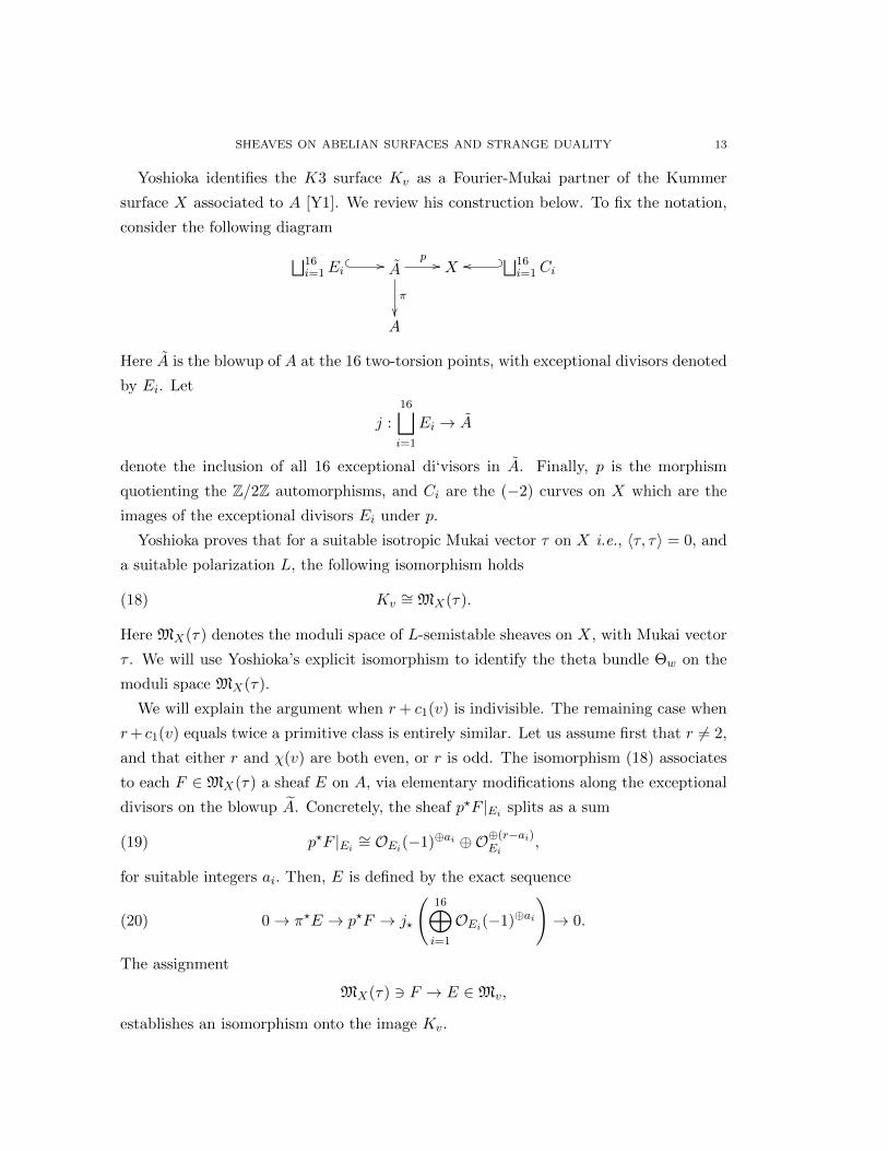
Yoshioka identifies the K3 surface Kv as a Fourier-Mukai partner of the Kummer

surface X associated to A [Y1]. We review his construction below. To fix the notation,

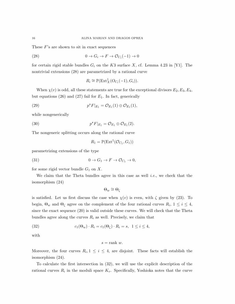
consider the following diagram⊔16i=1Ei

� � // Ap //

π

��

X⊔16i=1Ci

? _oo

A

Here A is the blowup of A at the 16 two-torsion points, with exceptional divisors denoted

by Ei. Let

j :16⊔i=1

Ei → A

denote the inclusion of all 16 exceptional di‘visors in A. Finally, p is the morphism

quotienting the Z/2Z automorphisms, and Ci are the (−2) curves on X which are the

images of the exceptional divisors Ei under p.

Yoshioka proves that for a suitable isotropic Mukai vector τ on X i.e., 〈τ, τ〉 = 0, and

a suitable polarization L, the following isomorphism holds

(18) Kv∼= MX(τ).

Here MX(τ) denotes the moduli space of L-semistable sheaves on X, with Mukai vector

τ . We will use Yoshioka’s explicit isomorphism to identify the theta bundle Θw on the

moduli space MX(τ).

We will explain the argument when r+ c1(v) is indivisible. The remaining case when

r+ c1(v) equals twice a primitive class is entirely similar. Let us assume first that r 6= 2,

and that either r and χ(v) are both even, or r is odd. The isomorphism (18) associates

to each F ∈MX(τ) a sheaf E on A, via elementary modifications along the exceptional

divisors on the blowup A. Concretely, the sheaf p?F |Ei splits as a sum

(19) p?F |Ei∼= OEi(−1)⊕ai ⊕O⊕(r−ai)

Ei,

for suitable integers ai. Then, E is defined by the exact sequence

(20) 0→ π?E → p?F → j?

(16⊕i=1

OEi(−1)⊕ai

)→ 0.

The assignment

MX(τ) 3 F → E ∈Mv,

establishes an isomorphism onto the image Kv.


In fact, Yoshioka’s construction works in families, giving a natural transformation

between the moduli functors

MX(τ)→ Kv.

The exact description of this transformation will be useful later. In what follows, let us

agree that the base change of various morphisms to an arbitrary base S will be decorated

by overlines. Fix any flat S-family F of sheaves in MX(τ)(S). Define the sheaf G on the

union⊔16i=1Ei × S via the exact sequence

(21) 0→ π?π?j?p?F → j?p?F → G → 0.

The short exact sequence

(22) 0→ π?E → p?F → j?G → 0

then defines a new S-family E in Kv(S).

Now let

(23) ζ = ch (p! (π?W )) (1 + ω) ∈ H?(X),

be the Mukai vector of the pushforward p!(π?W ), for an arbitrary sheaf W on A with

Mukai vector w. Using the exact sequence (20), and the fact that

χ(j?OEi(−1)⊗ π?w) = 0,

we find

2χ(τ ⊗ ζ) = χ(p?τ ⊗ π?w) = χ(π?(v ⊗ w)) = χ(v ⊗ w) = 0.

The above computation shows that ζ defines a Theta line bundle Θζ on MX(τ). We

claim that under the isomorphism Kv∼= MX(τ) we have an identification

(24) Θw∼= Θζ .

As for any good quotient, the Picard group of the moduli scheme MX(τ) injects into

that of the moduli functor MX(τ). Therefore, it suffices to check equality of the two

line bundles Θw and Θζ over arbitrary base schemes S, and for arbitrary S-families Fof MX(τ).

Let q : S × A → S and q : S × X → S be the two projections. The exact sequence

(22) and the push-pull formula then give

Θw = det Rq! (π?E ⊗ pr?Aw)−1 = det Rq! (p?F ⊗ pr?Aw)−1 = det Rq! (F ⊗ pr?Xζ)−1 = Θζ .

Here, we used that the contribution of the last term of (22) vanishes. Indeed, since

j?pr?Aw = rank (w) · 1,


we have

det Rq! (j?G ⊗ pr?Aw) = rank (w) · det R (qj)! (G) = 0.

The last equality follows from the fact that all direct images of G vanish. This is implied

by the base change theorem, observing that the restriction of G to each fiber of the

morphism qj : S × Ei → S splits as a sum of line bundles OEi(−1). In turn this latter

fact is a consequence of the defining exact sequence (22), in conjunction with equation

(19).

To complete the proof, recall that Mukai [Muk4] established an isometric isomorphism

H2(MX(τ)) ∼= τ⊥/τ

where the left hand side is endowed with the intersection pairing, while the right hand

side carries the Mukai form induced from the cohomology H?(X). Then,

c1(Θw)2 = c1 (Θζ)2 = 〈ζ, ζ〉 = 2〈w,w〉.

This proves (17).

The case r 6= 2 and χ(v) odd is entirely similar. In this case, the exact sequence (20)

is replaced by

0→ π?E → p?F (E1)→ j?

(16⊕i=1

OEi(−1)⊕ai

)→ 0.

The argument identifying the Theta bundles carries through, for the vector

(25) ζ = ch(p!(π?W (E1))(1 + ω).

The case r = 2 requires a different discussion, since in this case, the description of the

isomorphism (18) via the assignment F → E is valid only on the complement of four

rational curves Ri, 1 ≤ i ≤ 4. In fact, one cannot pick an isotropic vector τ such that for

each of the 16 exceptional divisors, the splitting type (19) is independent of the choice

of a point [F ] ∈MX(τ). At best, for a suitable τ , the rigid splitting

p?F |Ei∼= OEi ⊕OEi(−1)

holds for 12 exceptional divisors Ei, 5 ≤ i ≤ 16. For the remaining four divisors Ei, 1 ≤i ≤ 4, the splitting type varies within the moduli space.

When χ(v) is even, for generic F in MX(τ), the splitting type is

(26) p?F |Ei = OEi ⊕OEi , 1 ≤ i ≤ 4.

The loci of non-generic splitting give rational curves Ri in Kv. Indeed, the nongeneric

splitting is

(27) p?F |Ei = OEi(−1)⊕OEi(1).


These F ’s are shown to sit in exact sequences

(28) 0→ Gi → F → OCi(−1)→ 0

for certain rigid stable bundles Gi on the K3 surface X, cf. Lemma 4.23 in [Y1]. The

nontrivial extensions (28) are parametrized by a rational curve

Ri ∼= P(Ext1X(OCi(−1), Gi)).

When χ(v) is odd, all these statements are true for the exceptional divisors E2, E3, E4,

but equations (26) and (27) fail for E1. In fact, generically

(29) p?F |E1 = OE1(1)⊕OE1(1),

while nongenerically

(30) p?F |E1 = OE1 ⊕OE1(2).

The nongeneric splitting occurs along the rational curve

R1 = P(Ext1(OC1 , G1))

parametrizing extensions of the type

(31) 0→ G1 → F → OC1 → 0,

for some rigid vector bundle G1 on X.

We claim that the Theta bundles agree in this case as well i.e., we check that the

isomorphism (24)

Θw∼= Θζ

is satisfied. Let us first discuss the case when χ(v) is even, with ζ given by (23). To

begin, Θw and Θζ agree on the complement of the four rational curves Ri, 1 ≤ i ≤ 4,

since the exact sequence (20) is valid outside these curves. We will check that the Theta

bundles agree along the curves Ri as well. Precisely, we claim that

(32) c1(Θw) ·Ri = c1(Θζ) ·Ri = s, 1 ≤ i ≤ 4,

with

s = rank w.

Moreover, the four curves Ri, 1 ≤ i ≤ 4, are disjoint. These facts will establish the

isomorphism (24).

To calculate the first intersection in (32), we will use the explicit description of the

rational curves Ri in the moduli space Kv. Specifically, Yoshioka notes that the curve


Ri corresponds to those sheaves E on A which fail to be locally free at a two-torsion

point xi. We can construct these sheaves as elementary modifications of a fixed V :

(33) 0→ E → V → O{xi} → 0.

The middle sheaf V has Mukai vector v + ω, so it sits in a moduli space of dimension

2. We may assume that V is locally free at xi; this may be arranged by starting with

an arbitray V with Mukai vector v + ω, and then pulling back by a translation on the

abelian variety A, if necessary to obtain local-freeness at xi. With this understood, it

follows that E is not locally free at xi. The nonlocally free elementary modifications E

are parametrized by a P1, which should therefore be the rational curve Ri above.

The universal structure on Ri × A, associated to the elementary modifications (33),

becomes

0→ E → pr?AV → ORi(1) �O{xi} → 0.

Therefore,

c1(Θw) ·Ri = −c1(p!(E ⊗ pr?Aw)) = c1

(p!

(ORi(1) �

(O{xi} ⊗ w

)))= c1(ORi(1)⊕s) = s.

To prove the second equality of (32), we will use the description of the rational curves

Ri provided by equation (28). The universal extension

0→ pr?XGi → F → ORi(−1) �OCi(−1)→ 0

on Ri ×X restricts to (28) on the fibers of the projection p : Ri ×X → Ri. Using this

exact sequence, we compute

c1(Θζ) ·Ri = −c1(p!(F ⊗ pr?Xζ)) = −c1 (p! (ORi(−1) � (OCi(−1)⊗ ζ)))

= −c1(ORi(−1))χ(OCi(−1)⊗ ζ) = c1(ζ) · Ci = s.

The last evaluation follows from (23) via Riemann-Roch.

When χ(v) is odd, the numerics are slightly different, but (24) still holds for the vector

ζ given by (25). In this case, we check that

c1(Θζ) ·R1 = s,

using equation (31), instead of (28).

Finally, to see that the curves Ri’s are disjoint, assume for a contradiction that the

intersection of Ri and Rj contains a sheaf E, for i 6= j. It follows that E fails to be

locally free at two different two-torsion points. Then the quotient E∨∨/E is supported

at least at two points. Thus, E∨∨ has Mukai vector v+aω, for a ≥ 2. Its self-intersection

is

〈v(E∨∨), v(E∨∨)〉 = 〈v, v〉 − 4a = 4− 4a ≤ −4.


This contradicts the Bogomolov inequality for the vector bundle E∨∨, proving our claim.

This completes our analysis of the two-dimensional Albanese fibers, establishing Propo-

sition 1.

4. Sheaves with fixed determinant

In this section we will prove Theorem 1. We begin by fixing the notation. Specifically,

let us write r,Λ, χ for the rank, determinant and Euler characteristic of the vector v. The

notation r′,Λ′, χ′ will be used for the vector w. The orthogonality of v and w translates

into

(34) r′χ+ c1(Λ) · c1(Λ′) + rχ′ = 0.

Let P be the normalized Poincare bundle on A× A. We make the convention that x will

stand for a point of A, while y will be a point of A. We will write

Px = P|{x}×A, Py = P|A×{y} ∼= y.

We denote by tx and ty the translations by x and y on the abelian varieties A and A

respectively.

The following two facts about the Fourier-Mukai transform of an arbitrary E ∈ D(A),

proved in [Muk2], will be used below:

(35) RS(E ⊗ Py) = t?y RS(E),

(36) RS(t?xE) = RS(E)⊗ P−x.

It is moreover useful to recall that the two line bundles Λ and Λ standardly induce

morphisms

ΦΛ : A→ A, x 7→ t?xΛ⊗ Λ−1, and

ΦΛ

: A→ A, y → t?yΛ⊗ Λ−1,

satisfying [Y1]

(37) ΦΛ ◦ ΦΛ

= −χ(Λ)1, ΦΛ◦ ΦΛ = −χ(Λ)1.

To start the proof of Theorem 1, consider the diagram

Kv ×AΦ+

//

p

��

M+v

α−

��A

Ψ+// A

.


The upper horizontal map is given by

Φ+(E, x) = t?rxE ⊗ t?xΛ−1 ⊗ Λ.

This is well defined since

det Φ+(E, x) = t?rxΛ⊗(txΛ−1 ⊗ Λ

)r= Λ.

Lemma 3. The morphism Ψ+ is the multiplication by dv in the abelian variety.

Proof. Using (35) and (36), we compute

α− ◦ Φ+(E, x) = det RS(t?rxE ⊗ t?xΛ−1 ⊗ Λ)⊗ Λ−1 = det RS(t?rxE ⊗ P−ΦΛ(x))⊗ Λ−1

= det(t?−ΦΛ(x)RS(t?rxE)

)⊗ Λ−1 = t?ΦΛ(−x) det RS(t?rxE)⊗ Λ−1

= t?ΦΛ(−x) det (RS(E)⊗ P−rx)⊗ Λ−1

= t?ΦΛ(−x)

(det RS(E)⊗ Pχ−rx

)⊗ Λ−1

= t?ΦΛ(−x)Λ⊗ P−rχx ⊗ Λ−1 = ΦΛ

(ΦΛ(−x))⊗ P−rχx= χ(Λ)x⊗ P−rχx = (χ(Λ)− rχ)x = dvx.

The first equality on the penultimate line follows from the fact that the Poincare bundle

Px is invariant under translations [M]. Equation (37) was used in the last line.

Lemma 4. When dv 6= 0, the diagram above is cartesian. Therefore, the morphism Φ+

has degree d4v.

Proof. This is almost immediate. Together, Φ+ and p give rise to a morphism

i : Kv ×A→ M+v ×A,(α−,Ψ+) A.

We show that i is an isomorphism. Since Ψ+ is etale, the natural morphism

M+v ×A,(α−,Ψ+) A→ M+

v

is also etale, so the fibered product M+v ×A,(α−,Ψ+) A is smooth. The fibered product is

also connected, as it follows by looking at the connected fibers of the projection to A;

note that the projection is surjective, as α− has this property, according to the previous

Lemma. Therefore, it suffices to check that i is injective. If i(E, x) = i(E′, x′) then, by

composing i with Φ+ and p, we see that

t?rxE ⊗ t?xΛ−1 ⊗ Λ = t?rx′E′ ⊗ t?x′Λ−1 ⊗ Λ, and x = x′.

This immediately implies E = E′ as well. The diagram is therefore cartesian.


Proposition 2. We have (Φ+)?

Θw∼= Θw � L+

where L+ is a line bundle on A with

c1(L+) = dvc1(v ⊗ w).

Proof. This follows by the see-saw theorem. Letting Φx = Φ+|Kv×{x}, we claim that the

pullback Φ?xΘw is independent of x, and therefore, by specializing to x = 0, it should

coincide with Θw. Since Kv is simply connected, it suffices to check that the Chern class

c1(Φ?xΘw) is independent of x. This is clear when a universal sheaf E exists on M+

v ×A.Indeed, for F a sheaf on A with Mukai vector w,

Φ?xΘw = Φ?

x (det Rp!(E ⊗ q?F ))−1 =(det Rp!

((1× trx)?E ⊗ q?

(t?xΛ−1 ⊗ Λ⊗ F

)))−1.

The first Chern class can then be computed by Grothendieck-Riemann-Roch. The an-

swer does not depend on the point x ∈ A since the maps (1 × trx)? and t?x act as the

cohomological restriction associated with Kv ×A ↪→ M+v ×A, and as the identity on the

cohomology of A, respectively. When a universal family does not exist, one can use a

quasi-universal family instead.

The above argument shows that (Φ+)?

Θw should be of the form Θw � L+ for some

line bundle L+ coming from A. We can express this line bundle explicitly as follows.

Write

m = m1 : A×A→ A, (a, b)→ a+ b

for the addition map, and consider the morphism

mr : A×A→ A, (a, b)→ a+ rb.

Then,

mr = m ◦ (1, r).

Letting p1, p2 be the two projections, we have

L+ =(det Rp2!

(m?rE ⊗m?Λ−1 ⊗ p?1(Λ⊗ F )

))−1.

Letting λ = c1(Λ), we get by Grothendieck-Riemann-Roch,

c1(L+) = −p2!

[m?rv ·m?e−λ · p?1(eλw)

](3).

Expanding each of the terms, we obtain

c1(L+) = −p2!

[(r +m?

rλ+ χm?rω) ·

(1−m?λ+

λ2

2m?ω

)·p?1(r′ +

(r′λ+ λ′

)+

(χ′ + λλ′ + r′

λ2

2

)ω

)](3)

.


The precise evaluation of this product relies on the following intersections

p2!(m?λ · p?1ω) = λ, p2!(m

?rλ · p?1ω) = r2λ,

p2!(m?rω ·m?λ) = (r − 1)2λ, p2!(m

?rλ ·m?ω) = (r − 1)2λ,

p2!(m?ω · p?1α) = α, p2!(m

?rω · p?1α) = r2α, for any α ∈ H2(A).

The last pair of intersections is to be used for the class α = r′λ + λ′. The formulas

above are easily justified either by explicit computations in coordinates, or directly, by

interpreting geometrically the intersections involved. For instance, the third pushforward

p2!(m?rω ·m?λ) is computed as the image under p2 of the cycle

{(a, b), a+ rb = 0, a+ b ∈ λ} ↪→ A×A.

This pushforward can be identified with (r − 1)?λ = (r − 1)2λ.

The value of the Chern class is obtained immediately from the previous intersections

and a last one calculated by the Lemma below. Equation (34) has to be used to bring

the answer in the form claimed by Proposition 2.

Lemma 5. For any λ, α ∈ H2(A), we have

p2!(m?rλ ·m?λ · p?1α) = (r − 1)2

(∫Aαλ

)· λ+ rλ2 · α.

Proof. First, note the isomorphism

m?Λ ∼= p?1Λ⊗ p?2Λ⊗ (1× ΦΛ)?P.

This shows that

(38) m?λ = p?1λ+ p?2λ+ (1× ΦΛ)?c1(P), and

m?rλ = (1× r)?m?λ = p?1λ+ r2p?2λ+ r · (1× ΦΛ)?c1(P).

It follows that

p2!(m?rλ ·m?λ · p?1α) = (r2 + 1)

(∫Aαλ

)· λ+ r · p2!

(p?1α · (1× ΦΛ)?c1(P)2

)= (r2 + 1)

(∫Aαλ

)· λ+ 2r · Φ?

Λ

{p2!

(p?1α ·

c1(P)2

2

)}.

We will prove

(39) Φ?Λ

{p2!

(p?1α ·

c1(P)2

2

)}= −

(∫Aαλ

)· λ+

λ2

2· α.

This follows by a computation in coordinates. Explicitly, let us write A = V/Γ.

We regard V as a four-dimensional real vector space. The dual abelian variety has as


underlying real manifold the torus V ∨/Γ∨, where V ∨ stands for the real dual of V . Pick

a basis f1, f2, f3, f4 for V , which is symplectic for Λ. This means that in the dual basis,

λ = c1(Λ) = d · f∨1 ∧ f∨2 + e · f∨3 ∧ f∨4 ∈ Λ2V ∨,

for some (integers) d and e. Moreover, the Chern class of the Poincare line bundle on

A× A takes the form

(40) c1(P) = f∨1 ∧ f1 + f∨2 ∧ f2 + f∨3 ∧ f3 + f∨4 ∧ f4.

Note that pullbacks of the 1-forms f∨i and fi from the two factors A and A to their

product are understood in the above equation. Throughout the paper, it should be clear

from the context when such notational simplifications are employed.

To prove (39), it suffices to assume that

α = f∨1 ∧ f∨2 , or α = f∨1 ∧ f∨3 .

Let us consider only the first case, the second being similar. Then,

p2!

(p?1α ·

c1(P)2

2

)= −f3 ∧ f4.

The discussion in [LB], chapter 2, and in particular Lemma 4.5 therein, shows that the

map

Φ?Λ : H1(A,R) ∼= V → H1(A,R) ∼= V ∨

is induced by the contraction of the first Chern class c1(Λ). It follows that

Φ?Λ

{p2!

(p?1α ·

c1(P)2

2

)}= −Φ?

Λf3 ∧ Φ?Λf4 = −e2 f∨3 ∧ f∨4 .

But this is also the result on the right hand side of (39):

−(∫

Aαλ

)· λ+

λ2

2· α = −e · λ+ de · α = −e2 f∨3 ∧ f∨4 .

Proof of Theorem 1. When dv 6= 0, Theorem 1 follows immediately from Propositions

1 and 2, and Lemma 4. Indeed, we have

χ(M+v ,Θw) =

1

d4v

χ((Φ+)?

Θw) =1

d4v

χ(Kv,Θw)χ(A,L+)

=1

d4v

· d2v

dv + dw

(dv + dwdv

)· (dvc1(v ⊗ w))2

2=

1

2

c1(v ⊗ w)2

dv + dw

(dv + dwdv

).

When dv = 0, the Theorem is equivalent to the equality

χ(M+v ,Θw) = r2.


It suffices to explain that the moduli space M+v consists of r2 smooth points. By work

of Mukai, it is known that Mv is an abelian surface. In fact, fixing E ∈ M+v , we have an

isogeny

A→Mv, x→ t?xE,

whose kernel is the group

K(E) = {x ∈ A such that t?xE∼= E} .

Note that we may need to replace E by a twist E ⊗H⊗n to ensure that K(E) is finite.

In this case, K(E) has χ2 elements. This is a result of Mukai [Muk1]; to apply it, we

need to observe that E is a simple semi-homogeneous sheaf. Restricting to sheaves with

determinant Λ, we see that

M+v∼= K(Λ)/K(E),

has length χ(Λ)2

χ2 = r2.

5. Sheaves with fixed determinant of the Fourier-Mukai transform.

This section is devoted to the proof of Theorem 2. It is possible to deduce this result

from Theorem 1 when the Picard number of A is 1, by explicitly studying how the

relevant moduli spaces and Theta divisors change under the Fourier-Mukai transform

[Y1][Ma]. However, the following proof is simpler, covers all cases, and it is in the spirit

of this paper. Note that the cohomological computation below may be regarded as the

Fourier-Mukai ’dual’ of last section’s calculations.

We will crucially make use of the diagram

Kv × AΦ− //

p

��

M−v

α+

��

AΨ− // A

.

The upper horizontal morphism Φ− is defined as

Φ−(E, y) = t?ΦΛ

(y)E ⊗ yχ.

To check that Φ− is well defined, we compute

det RS(Φ−(E, y)

)= det RS

(t?Φ

Λ(y)E ⊗ y

χ)

= det(t?χy RS(E)⊗ Φ

Λ(y)−1

)= t?χy det RS(E)⊗ Φ

Λ(y)−χ = t?χyΛ⊗ Φ

Λ(y)−χ

= Λ⊗ ΦΛ

(χy)⊗ ΦΛ

(y)−χ = Λ.


The next two results are the versions of Lemma 3 and Proposition 2 suitable to the

present context.

Lemma 6. The morphism Ψ− is the multiplication by −dv on the abelian variety A.

Proof. Using (36) and (37), we compute

α+ ◦ Φ−(E, y) = det(t?Φ

Λ(y)E ⊗ y

χ)⊗ Λ−1 = t?Φ

Λ(y)Λ⊗ y

rχ ⊗ Λ−1

= ΦΛ

(Φ

Λ(y))⊗ yrχ = (−χ(Λ) + rχ)y = −dvy.

Proposition 3. We have (Φ−)?

Θw∼= Θw � L−,

where

c1(L−) = −dvc1(v ⊗ w).

Proof. The proof of this result parallels that of Proposition 2. It suffices to show that

the line bundle L− corresponding to the divisor{y ∈ A, with H0

(t?Λ(y)

(E)⊗ yχ ⊗ F)6= 0}

has the first Chern class given by the Proposition. Note that

L− = (det p2! (f?E ⊗ p?1F ⊗ Pχ))−1 ,

where

f : A× A→ A×A→A

denotes the composition

(41) f = m ◦ (1× ΦΛ

), (x, y)→ x+ ΦΛ

(y).

By Riemann-Roch, we compute

c1(L−) = −p2!

[(r + f?λ+ χf?ω) ·

(r′ + p?1λ

′ + χ′p?1ω)·(

1 + χc1(P) + χ2 c1(P)2

2

)](3)

.

The following observations allow for the explicit evaluation of the expression above:

p2!

(c1(P)2

2· p?1λ′

)= λ′, p2!

(c1(P)2

2· f?λ

)= λ,

(42) p2!(f?ω · p?1λ′) =

λ2

2· λ′ − (λ · λ′) · λ,

(43) p2! (f?λ · p?1ω) = −λ2

2· λ,

(44) p2! (f?ω · c1(P)) = −2λ,


(45) p2!

(f?λ · p?1λ′ · c1(P)

)= −λ2 · λ′.

The Proposition follows by substitution, also making straightforward use of the orthog-

onality constraint

rχ′ + λ · λ′ + r′χ = 0.

It remains to explain the four numbered equations claimed above. Let us first consider

(42). Interpreting the pushforward geometrically, and recalling the definiton of f in (41),

we find that

p2!(f?ω · p?1λ′) = (−Φ

Λ)?λ′ = Φ?

Λλ′ =

λ2

2· λ′ −

(∫Aλ · λ′

)· λ.

The dual of the last equality was verified in (39). The case at hand is a corollary of

what we have already shown there, using the fact that the Fourier-Mukai transform is

an isometry. Equation (43) is very similar. To prove it, we observe that f restricts to

ΦΛ

on {0} × A, hence

p2! (f?λ · p?1ω) = Φ?Λλ = −λ

2

2· λ.

In turn, (44) follows by a computation in local coordinates. First, pick a basis

f1, f2, f3, f4 for V such that

c1(P) = f∨1 ∧ f1 + f∨2 ∧ f2 + f∨3 ∧ f3 + f∨4 ∧ f4.

From the definition of f in (41), we calculate

p2!(f?ω · c1(P)) = p2!

((1× Φ

Λ)?m?ω · c1(P)

)=

= −p2!

(1× ΦΛ

)?

4∑j=1

PD(f∨j ) ∧ f∨j

· 4∑j=1

f∨j ∧ fj

=4∑j=1

Φ?Λf∨j ∧ fj .

Taking

λ = d · f∨1 ∧ f∨2 + e · f∨3 ∧ f∨4 ,

this last expression is

(46) 2d · f3 ∧ f4 + 2e · f1 ∧ f2 = −2λ,

confirming (44).

Finally, for (45), we observe that

p2!

(f?λ · p?1λ′ · c1(P)

)= p2!

((1× Φ

Λ)?m?ω · p?1λ′ · c1(P)

)= p2!

((1× Φ

Λ)?(1× ΦΛ)?c1(P) · p?1λ′ · c1(P)

)= p2! ((1× (−χ(Λ)))? c1(P) · p?1λ′ · c1(P))

= −χ(Λ) · p2!(c1(P)2 · p?1λ′) = λ2 · λ′.


The first line follows by the definition of f in (41), the second uses (38), while the third

uses (37).

Proof of Theorem 2. As before, when dv 6= 0, the Theorem follows immediately from

Propositions 1 and 3, and Lemma 6. Using the cartesian diagram, we compute

χ(M−v ,Θw) =1

d4v

χ((Φ−)?

Θw) =1

d4v

χ(Kv,Θw)χ(A,L−)

=1

d4v

· d2v

dv + dw

(dv + dwdv

)· (dvc1(v ⊗ w))2

2=

1

2

c1(v ⊗ w)2

dv + dw

(dv + dwdv

).

When dv = 0, we observe that M−v consists of χ2 smooth points. First, for any sheaf

E in the moduli space Mv, consider the isogeny

A→Mv, y 7→ E ⊗ Py.

The kernel

Σ(E) ={y ∈ A such that E ⊗ Py ∼= E

}has length r2, cf. [Muk1] (as in the proof of Theorem 1, twisting by powers of H may

be necessary). Note that the points in M−v have the property

det RS (E ⊗ Py)⊗ (det RSE)−1 ∼= t?yΛ⊗ Λ−1 ∼= O.

Therefore,

M−v = K(Λ)/Σ(E)

has length χ(Λ)2/r2 = χ2, as claimed.

6. Sheaves with arbitrary determinant.

This last section contains the proof of Theorem 3. The Euler characteristic on Kv was

calculated in Proposition 1. To compute the one on Mw, we use the diagram

Kw ×A× AΦ //

p

��

Mw

aw��

A× AΨ // A× A

.

Here, Φ : Kw ×A× A→Mw is defined as

Φ(E, x, y) = t?xE ⊗ y.

Using (35) and (36), Yoshioka proved in detail that

Ψ(x, y) = (−χ′x+ ΦΛ′(y),ΦΛ′(x) + r′y),

which has degree d4w [Y1].


Proposition 4. We have

Φ?Θv = Θv � L

where L is a line bundle on A× A with

χ(L) = d2vd

2w.

Proof. It suffices to compute the Euler characteristic of the line bundle L corresponding

to the divisor

{(x, y) ∈ A× A, such that H0(t?xE ⊗ y ⊗ F ) 6= 0}.

In other words

L = (det p23! (m?12E ⊗ p?13P ⊗ p?1F ))−1 ,

where the p’s denote the projections on the corresponding factors of A×A× A, while

m12 : A×A× A→ A

is the addition on the first two factors. Keeping the previous notations,

c1(L) = −p23!

[(r +m?

12λ+ χm?12ω) ·

(1 + p?13c1(P) +

p?13c1(P)2

2

)·(r′ + p?1λ

′ + χ′p?1ω)]

(3)

.

Expanding, we easily obtain

−c1(L) = (χλ′ + χ′λ) + (rλ′ + r′λ)− rχ′c1(P) + p23!

(m?

12λ · p?13c1(P) · p?1λ′).

We claim that

χ(L) =c1(L)4

4!= d2

vd2w.

The computation makes use of the fact that the Picard number of A is 1, so we may

assume that either λ′ = 0, or otherwise that

λ = aλ′

for some constant a. In the first case, we have

c1(L) = −χ′λ− r′λ+ rχ′c1(P).

To prove the claim, we first note that

(47) λ · λ · c1(P)2

2= λ2

This follows easily by a computation in local coordinates. Indeed, writing

(48) λ = d · f∨1 ∧ f∨2 + e · f∨3 ∧ f∨4 ,

and recalling that λ and c1(P) have the form (46) and (40) respectively, we calculate

λ · λ · c1(P)2

2= 2de = λ2.


With (47) understood, and using the fact that the Fourier-Mukai is an isometry, we

obtain

c1(L)4

4!=

1

4!(χ′λ+ r′λ− rχ′c1(P))4 =

r′2χ′2(λ2)2

4+ r′χ′(rχ′)2λ2 + (rχ′)4

=

(r′χ′λ2

2+ (rχ′)2

)2

=

[r′χ′

(λ2

2− rχ

)]2

= d2vd

2w.

The penultimate equality made use of the fact that rχ′ + r′χ = 0.

Finally, the more general second case λ = aλ′ is similar. Using (38), we get

p23!

(m?

12λ · p?13c1(P) · p?1λ′)

= (ΦΛ × 1)?q23!

(q?12c1(P) · q?13c1(P) · q?1λ′

),

with the q’s standing for the projections of the factors of A× A× A. In turn, we claim

that

(49) (ΦΛ × 1)?q23! (q?12c1(P) · q?13c1(P) · q?1λ) = −λ2

2c1(P).

Again, this is easiest to check in local coordinates. Assuming that (48) holds, we have

q23! (q?12c1(P) · q?13c1(P) · q?1λ) = −d · f3 ∧ f4 + d · f4 ∧ f3 − e · f1 ∧ f2 + e · f2 ∧ f1.

Note that here we follow our previous notational conventions; in particular, pullbacks of

the 1-forms fi from the two factors of A×A are understood in the above wedge products.

After pullback by ΦΛ × 1, the left hand side of (49) becomes

−de c1(P) = −λ2

2c1(P),

as claimed. Putting things together, we obtain

c1(L) = −(χ′a+ χ)λ′ − (r′a+ r)λ′ +

(rχ′ +

aλ′2

2

)c1(P).

The same type of calculation as the one done above yields the answer

χ(L) =c1(L)4

4!=

(χ′a+ χ)(r′a+ r)λ′2

2+

(rχ′ +

aλ′2

2

)22

.

To conclude the proof, it remains to observe that the expression in square brackets can

be equated with

−(a2λ′2

2− rχ

)(λ′2

2− r′χ′

)= −dvdw,

so that

χ(L) = (dvdw)2.

The latter algebraic manipulation will be left to the reader, who may wish to use the

fact that

aλ′2 + rχ′ + r′χ = 0.


It is very likely that the Lemma holds true for arbitrary abelian surfaces, without any

restrictions on the Neron-Severi group, but the computation seems to be more involved.

Proof of Theorem 3. We compute

χ(Mw,Θv) =1

d4w

χ(Kw,Θv)χ(A× A,L) =1

d4w

· d2w

dv + dw

(dv + dwdv

)·(d2vd

2w

)=

d2v

dv + dw

(dv + dwdv

)= χ(Kv,Θw).

The case dw = 0 requires, as usual, special care. We need to show

χ(Mw,Θv) = dv.

Using the degree χ′2 isogeny:

π : A→Mw, x→ t?xF,

where F is a semi-homogeneous sheaf of Mukai vector w, we have

π?Θv = (det p!(m?F ⊗ q?E))−1 ,

with p, q and m standing for the projection and addition morphism. Then

c1(π?Θv) = −χ′λ− χλ′.

We obtain

χ(Mw,Θv) =1

χ′2χ(A, π?Θv) =

1

2χ′2(χ′λ+χλ′)2 =

1

2χ′2(χ′2λ2 + χ2λ′2 − 2χχ′(rχ′ + r′χ)

)=

1

χ′2(χ2dw + χ′2dv) = dv.

This completes the proof of the Theorem.

References

[B] P. Belkale, The strange duality conjecture for generic curves, J. Amer. Math. Soc. 21 (2008), no. 1,235-258.

[BN] M. Britze, M. Nieper, Hirzebruch-Riemann-Roch formulae on irreducible symplectic Kahler mani-folds, preprint, arXiv:math/0101062.

[D] G. Danila, Resultats sur la conjecture de dualite etrange sur le plan projectif, Bull. Soc. Math. France,130 (2002), no. 1, 1-33.

[DN] J. M. Drezet, M.S. Narasimhan, Groupe de Picard des varietes de modules de fibres semi-stablessur les courbes algebriques, Invent. Math. 97 (1989), no. 1, 53-94.

[EGL] G. Ellingsrud, L. Gottsche, M. Lehn, On the cobordism class of the Hilbert scheme of a surface,J. Algebraic Geom. 10 (2001), 81-100.

[GNY] L. Gottsche, H. Nakajima, K. Yoshioka, K-theoretic Donaldson invariants via instanton counting,arXiv:math/0611945.

[HT] B. Hassett, Y. Tschinkel, Moving and ample cones of holomorphic symplectic fourfolds,arXiv:0710.0390.

[H] D. Huybrechts, Compact Hyperkahler manifolds, Calabi-Yau manifolds and related geometries, Lec-tures from the Summer School held in Nordfjordeid, June 2001 Springer-Verlag, Berlin, 2003, 161-225.

[LB] H. Lange, C. Birkenhake, Complex abelian varieties, Springer-Verlag, Berlin-New York, 1992.


[LP] J. Le Potier, Fibre determinant et courbes de saut sur les surfaces algebriques, Complex ProjectiveGeometry, 213-240, London Math. Soc. Lecture Note Ser., 179, Cambridge Univ. Press, Cambridge,1992.

[Li] J. Li, Algebraic geometric interpretation of Donaldson’s polynomial invariants, J. Differential Geom.37 (1993), 417-466.

[MO1] A. Marian, D. Oprea, The level-rank duality for non-abelian theta functions, Invent. Math. 168(2007), 225-247.

[MO2] A. Marian, D. Oprea, A tour of theta dualities on moduli spaces of sheaves, to appear,arXiv:0710.2908.

[OG] K. O’Grady, Involutions and linear systems on holomorphic symplectic manifolds, Geom. Funct.Anal. 15 (2005), no. 6, 1223-1274.

[Ma] A. Maciocia, The determinant line bundle over moduli spaces of instantons on abelian surfaces,Math. Z. 217 (1994), no. 2, 317-333.

[Muk1] S. Mukai, Semi-homogeneous vector bundles on an Abelian variety, J. Math. Kyoto Univ. 18(1978), 239-272.

[Muk2] S. Mukai, Duality between D(X) and D(X) with its application to Picard sheaves, Nagoya Math.J. 81 (1981), 153-175.

[Muk3] S. Mukai, Symplectic structure of the moduli space of sheaves on an abelian or K3 surface, Invent.Math. 77 (1984), no. 1, 101-116.

[Muk4] S. Mukai, On the moduli space of bundles on K3 surfaces I, Vector bundles on algebraic varieties,Tata Institute for Fundamental Research Studies in Mathematics, no. 11 (1987), 341-413.

[M] D. Mumford, Abelian varieties, Tata Institute of Fundamental Research Studies in Mathematics,Oxford University Press, London, 1970.

[Y1] K. Yoshioka, Moduli spaces of stable sheaves on abelian surfaces, Math. Ann. 321 (2001), 817-884.[Y2] K. Yoshioka, Some notes on the moduli of stable sheaves on elliptic surfaces, Nagoya Math. J. 154

(1999), 73-102.

School of Mathematics

Institute for Advanced StudyE-mail address: [email protected]

Department of Mathematics

Stanford UniversityE-mail address: [email protected]

Sheaves on abelian surfaces and strange duality

Documents

Transcript of Sheaves on abelian surfaces and strange duality