arX

iv:h

ep-t

h/99

0623

5v4

25

Aug

200

0

hep-th/9906235ITEP-TH-36/96HUTP-97/A099

Duality in Integrable Systems and Gauge Theories

V. Fock1, A. Gorsky1, N. Nekrasov1,3, V. Rubtsov1,2

1,2,3 Institut Teoretiqeskoi i Зksperimentalьnoi Fiziki, 117259, Moskva, Rossi

3 Departement de Mathematiques, Universite d’Angers, 49045, Angers, France3 Lyman Laboratory of Physics, Harvard University, Cambridge MA 02138, USA

fock, gorsky@vitep5.itep.ru, nikita@bohr.harvard.edu, volodya@orgon.univ-angers.fr

We discuss various dualities, relating integrable systems and show that these dualities

are explained in the framework of Hamiltonian and Poisson reductions. The dualities we

study shed some light on the known integrable systems as well as allow to construct new

ones, double elliptic among them. We also discuss applications to the (supersymmetric)

gauge theories in various dimensions.

06/99

.

TABLE OF CONTENT

1. Introduction 2

2. The concepts of Duality 6

2.1 AC: (p, q) → (I, ϕ) 7

2.2 AA: I → ID 7

2.3 Quantum duality 8

3. Examples of dual systems. Two particles case. 10

3.1 Classical systems 10

3.2 Quantum systems 16

4. Duality in many-body systems 20

4.1 Examples. 20

4.2 Explanations: Hamiltonian and/or Poisson reductions 22

5. Gauge theories and duality in integrable systems 36

5.1 Old approach: many-body systems as low-dimensional

gauge theories 36

5.2. New approach: many-body systems in supersymmetric

gauge theories. 37

5.3 Duality in field theories vs. duality in many-body systems 38

1

1. Introduction

Traditionally the physical applications of integrable systems are exhausted by the

approximations to real dynamical systems. The configurations of the (classical or quantum)

model form the phase space which is a manifold M with the symplectic two-form ω or

Poisson bi-vector π.

The phase space might carry a natural complex structure, such that the symplectic

form ω is a holomorphic (2, 0)-form, the Hamiltonians H(p, q) are the holomorphic func-

tions and the vector fields are holomorphic vector fields (see [1] for example). The use of

integrable systems as describing the evolution in the physical models is less transparent in

this case.

The integrable systems in the holomorphic sense entered physics approximately at the

same time as the string theory did. Particle which has a one-real-dimensional worldline is

naturally described with the help of a real phase space, its (real) time evolution being gen-

erated by the real Hamiltonian. The worldsheet of a string is a complex curve, embedded

into the target space. It senses holomorphic geometry in many different ways. In partic-

ular, the embeddings of the worldsheet Σ are governed by a two dimensional conformal

field theory on Σ. An example of holomorphic integrable system relevant to the latter is

the famous Hitchin system. The phase space of this model is the cotangent bundle to the

moduli space MG(Σ) of holomorphic G-bundles over a Riemann surface Σ. One can think

of Knizhnik-Zamolodchikov-Bernard [2] equations in two dimensional WZW theories as of

the non-stationary quantum version of Hitchin system [3][4][5][6][7][8]. The role of times

is played by the complex (and hypothetically W)-moduli of Σ. Complex time evolution

occurs also in the models of N = (2, 2) strings, where space-time may have (2, 2) signature

[9].

However there exist other possibilities for integrable system to encode the physical

information.

In particular, the rich source of holomorphic integrable systems is the combination of

supersymmetry and duality. It is known for some time now that the holomorphy of certain

quantities (like the superpotential in N = 1 or prepotential in N = 2) in the supersym-

metric theories in three/four dimensions yields powerful predictions for the behavior of the

quantum theory even in the presence of the non-perturbative effects [10], [11], [12],[13],

[14], [15]. In particular, the complex structure of the moduli space of vacua in N = 4

3d gauge theories and N = 2 4d gauge theories can be determined revealing the exciting

2

link with the special nature of the geometry of the phase spaces of complex integrable

systems [16], [17], [18], [15]. The action variables appear as the central charges in the BPS

representations of the susy algebra [16].

There exists an approach to a class of integrable system which allows to uncover the

origin of their integrability/solvability. Namely, one realizes the system under investigation

as a projection of a simple system on a larger phase space [19],[20]. This idea is actually

a counterpart of the main principle behind the gauge theories - the complex dynamics

of the actual world (as far as most of the fundamental interactions are concerned) is a

projection of a somewhat simpler dynamics of the extended phase space. One of the goals

of the present discussion is to use the analogy between the two ideas and explain certain

properties of integrable systems as well as gauge theories.

We are going to study the phenomenon of duality whose precise definition is presented

shortly. Duality is a subject of much recent investigation in the context of (supersymmetric)

gauge theories, in which case the duality is an involution, which maps the observables of

one theory to those of another. The duality is powerful when the coupling constant in one

theory is inverse of that in another (or more generally, when small coupling is mapped

to the strong one). For example, a weakly coupled (magnetic) theory can be dual to the

strongly coupled (electric) theory thus making possible to understand the strong coupling

behavior of the latter. In particular, it was shown by N. Seiberg and E. Witten [12] that

using the concept of duality one can find exact low-energy Lagrangian of N = 2,d = 4

SU(2) gauge theory. A more fascinating recent development is that the duality connecting

weak and strong coupling regimes of one or different theories may have a geometric origin.

The most notorious example of that is provided by M -theory [21],[22]. We are going to

study the dualities in integrable systems, related to the gauge theories with the emphasis

on their geometric origin.

The study of geometry of integrable systems also allows to understand the origin of

certain constructions of separation of variables [23]. The similarity of this construction to

the description of the D2-brane moduli space and its role in the understanding the string

duality makes one hope that both subjects - many-body integrable systems and gauge

theories (more generally, D-geometry of M. Douglas [24][25]) will benefit more from each

other in the near future.

Topics left beyond the scope of the paper. To keep the size of the paper within

reasonable limits we decided to restrict our attention with the pure many-body systems.

More or less everything we have said can be carried over to the spin systems both of the

3

‘adjoint’ [26][27] and ‘fundamental’ [28] type. We don’t discuss extensively the relation

of our dualities in integrable systems to the physics of D-branes [29][30][31]. Some of

the results in this direction together with the applications to the theory of separation

of variables can be found in [23]. Also, except for the general discussion and two-body

examples we don’t treat quantum case. For some results related to our main topic see

[32][33][34][35]. Realizations of elliptic Ruijsenaars-Schneider models via Hamiltonian and

Poisson reductions can be found in [36].

Organization of the paper. Various concepts of duality are discussed in the section 2.

The examples of the dual systems are studied in section 3 where mostly two-body case is

treated, both classical and quantum one. Many-body systems are studied in the section

4 with the explanation of the dualities between them coming from Hamiltonian/Poisson

reductions. The section 5 is devoted to the gauge dynamics and their relation to the

integrable systems discussed so far. We discuss the geometry of the moduli spaces of vacua

of supersymmetric gauge theories in three, four, five and six dimensions and construct a

little dictionary translating the notions of integrable systems to those of gauge theories.

Acknowledgements. During the five years of the development of this project we have ben-

efited a lot from the discussions with our colleagues and friends on the matters reflected

in the paper. We are grateful to P. Cartier, P. Etingof, B. Enriquez, B. Feigin, G. Felder,

D. Ivanov, V. Kac, D. Kazhdan, B. Kostant, A. Kirillov, Jr., A. Losev, A. Rosly, S. Rui-

jsenaars, S. Shatashvili.

We would like to express our special gratitude to J. Harnad and M. Olshanetsky for

their interest and scepticism which helped us to finish this paper.

We would like to thank Institute of Theoretical Physics at Uppsala University, Institut

Mittag-Leffler and Antti Niemi for their hospitality when this project was launched and

finished.

In addition, A. G. thanks Institute of Theoretical Physics at University of Minnesota

and Institute of Theoretical Physics at Bern University where the part of the work was

done for the hospitality;

N. N. thanks CERN Theory Division and Prof. L. Alvarez-Gaume, Dept. of Math-

ematics at MIT and Prof. V. Guillemin, Dept. of Mathematics Yale University and

Profs. I. Frenkel and B. Khesin, Dept. of Mathematics at Brandeis University and Profs.

M. Adler, D. Buchsbaum, P. van Moerbeke, Institute of Theoretical Physics at University

of Minnesota and Profs. A. Vainshtein, M. Voloshin and M. Shifman, UNAM at Mexico

4

City and Prof. A. Turbiner, ITP at UC Santa Barbara and Prof. D. Gross for their hos-

pitality and the possibility to present some of the results of this paper there;

V. R. thanks CMAT Ecole Polytechniques, Universite Louis Pasteur Strasbourg I for

hospitality during preparation of the manuscript.

The preliminary results of the paper were reported at the conferences: International

Conference on String Theory, Quantum Gravity and Integrable Systems (Alushta, 1994,

1995), CIRM Colloquium “Geometrie symplectique d’espaces de modules et systemes in-

tegrables” (Luminy 1995), Workshop on Symplectic Geometry (MIT, 1995), Journee “Sys-

temes integrables et groupes quantiques” (Ecole Polytechnique Palaiseau, 1995), 33d Win-

ter School on String Theory and Duality (Karspasz, 1997), Workshop on Calogero-Moser-

Sutherland systems (CRM, Montreal, 1997), Journee “Geometrie algebrique, transforma-

tiones isomonodromiques et dualite” (Universite d’Artois, Lens, 1998)

We thank the organizers of the conferences for giving us the opportunity to present

our results there.

Research of A. G. was supported partially by the grants INTAS-97-0103 and Schweiz-

erisher Nationalfonds;

Research of N. N. was supported by Princeton University through Ogden Porter Jacobus

honorific fellowship, through the fellowship from Harvard Society of Fellows, partly by NSF

under the grants PHY-92-18167, PHY-94-07194, PHY-98-02709, partly by RFFI under

grant 96-02-18046;

N. N. and V. R are partly supported by the grant 96-15-96455 for scientific schools;

A. G ., V. F. and V. R. are partly supported by RFFI under grant 95-01-01110.

5

2. The concepts of Duality:

Let (M,ω) be a symplectic manifold. There exist Darboux local coordinates (cf. [37])

in which the symplectic form looks like a canonical one:

ω =

m∑

i=1

dpi ∧ dqi (2.1)

The local canonical coordinates are defined up to the symplectomorphisms. Unlike the gen-

eral diffeomorphisms, which have N functional degrees of freedom, N being the dimension

of the manifold, the symplectomorphisms have only 1 functional degree of freedom.

The evolution of a Hamiltonian system is defined with the help of Hamiltonian H :

M → IR. The function H defines a Hamiltonian vector field by the formula

ιVHω = −dH (2.2)

The integrable system on M has a maximal collection of the functionally independent

commuting Hamiltonians Hi i = 1, . . . , m = 12dimM :

[VHi, VHj

] = 0 (2.3)

Let ~h : M → B ≈ IRm be the map defined as: ~h : x 7→ (H1(x), . . . , Hm(x)). Liouville’s

theorem states that the integrable system has a normal form locally: there are coordinates

(Ii, ϕi), such that

ω =∑

i

dIi ∧ dϕi

Hk = fk(I)(2.4)

i.e. Ik are coordinates on B. For a sufficiently small domain U ⊂ B the space ~h−1(U) is

the product U×IRn−m×T 2m−n and ϕk are standard linear coordinates on IRn−m×T 2m−n.

If the common level set of all Hamiltonians is compact then this set is isomorphic to the

torus of the dimension m. In that case one may impose a condition on the coordinates

ϕi that the differentials dϕi have periods which are integer multiples of 2π. This fixes the

coordinates (I, ϕ) up to the action of discrete group PGLm(ZZ).

The Liouville theory also has a counterpart in the holomorphic setting where the

manifold M is replaced by the complex manifold, the symplectic form is a holomorphic

closed (2, 0)-form, the Hamiltonians H are the holomorphic functions and the vector fields

are holomorphic vector fields. The Liouville theorem modifies in this case. In fact the

6

Liouville real tori are replaced by the complex tori. If we require these tori to be abelian

varieties then we get what is called algebraically integrable system [38]. In the family of

such varieties the degenerate fibers can appear.

The coordinates Ii are referred to as “action” variables. If n = m then there is a nice

formula for I. Let b1, b2 ∈ U ⊂ B be sufficiently close to each other. Choose a basis eb in

IH1(~h−1(b1),ZZ). Connect the points b1 and b2 with a path γ ⊂ U . The base eb1 can be

transported to IH1(~h−1(γ),ZZ) by means of the Gauß-Manin connection and it defines an

element ~Γ ∈ IH2(~h−1(γ), ~h−1(b1 ∪ b2); ZZ). Then

~I(b2) − ~I(b1) =

∫

~Γ

ω

2.1. (p, q) → (I, ϕ)

Suppose that we have two integrable systems Hk and HDk on the same symplectic

manifold M . In this situation we say that these two systems are dual to each other.

Notice that this definition does not make duality an involution.

A pair of integrable systems given on one symplectic manifold (M,ω) is called self-dual

if there exists a symplectic involution σ : M → M exchanging Hk and HDk , i.e., such

that for any k = 1, . . . , n

σ∗Hk = HDk

Once we have two integrable systems on the same manifold such that both collections

of Hamiltonians constitute at least locally a coordinate system on the phase space M , one

can write down the equations of motion of the second integrable system in the second

order formalism using the action variables Ii of the first system as the coordinates qi for

the second.

The global version of this definition is: Two Hamiltonian systems are dual to each

other in the sense of action-coordinate (AC) duality if the action variables Ii of the first

system coincide with the coordinates qi of the second one and vice versa.

2.2. I → ID

In the holomorphic algebraic category there is an interesting complication: the torus

has a complex dimension m and therefore IH1(Tb; ZZ) = ZZ2m.

Again, let b1, b2 ∈ U ⊂ B be sufficiently close to each other. Choose a symplectic

basis eb1 = (Aα, Bβ) in IH1(~h

−1(b1),ZZ) such that A ∩ A = B ∩ B = 0, Aα ∩ Bβ = δβα,

7

where ∩ is an intersection form IH1 ⊗ZZ IH1 → ZZ. Connect the points b1 and b2 with a path

γ ⊂ U . The base eb1 can be transported to IH1(~h−1(γ),ZZ) by means of the Gauß-Manin

connection and it defines an element ~Γ ∈ IH2(~h−1(γ), ~h−1(b1∪b2); ZZ). The (A,B)-splitting

of the basis eb1 is also transported via Gauß-Manin along γ and defines the decomposition

~Γ = ~ΓA + ~ΓB , ~ΓA,B ∈ IH2(~h−1(γ), ~h−1(b1 ∪ b2); ZZ). Then define

~I(b2) − ~I(b1) =

∫

~ΓA

ω

~ID(b2) − ~ID(b1) =

∫

~ΓB

ω

(2.5)

We can take as the action variables the components of ~I. The reason for the B-cycles to be

discarded is simply the fact that the B-periods ~ID are not independent of the A-periods.

On the other hand, one can choose as the independent periods the integrals of ω over any

Lagrangian (in the sense of ∩) sublattice in IH1(Tb; ZZ) transported along γ.

This leads to the following structure of the action variables in the holomorphic setting.

Locally over a patch in B one chooses a basis in IH1 of the fiber together with the set of

A-cycles. This choice may differ over another patch. Over the intersection of these discs

one has a Sp2m(ZZ) transformation relating the bases. Altogether they form an Sp2m(ZZ)

bundle. It is an easy excercise on the properties of the period matrix of abelian varieties

that the two form:

dIi ∧ dIDi (2.6)

vanishes. Therefore one can always locally find a function F - prepotential, such that:

IDi =

∂F∂Ii

(2.7)

This duality maps the integrable system to itself. It is called action-action (AA) dual-

ity.

2.3. Quantum duality

There exists a clear quantum counterpart of this picture. Consider the eigenvalue

problem for the Schrodinger operators and the issue of the normalization of the wave-

functions.

The quantum integrable system is a complete collection of “independent” (in the

appropriate sense) commuting operators Hi, i = 1, . . . , m, acting in the Hilbert space

8

H of the model. By completeness we mean that these operators have simple common

spectrum U ⊂ IRm.The commuting operators have common eigenfunctions. Generically

the eigen-value problem:

Hk|~λ〉 = ek(λ)|~λ〉 (2.8)

has the unique (up to normalization) solution. Here ei is the corresponding eigenvalue

and ~λ is a label, which takes values in some set Λ. Altogether, ek form an imbedding

e∗ : Λ → U

Typically one has another set of commuting operators (“position operators”) HDk

and the eigen-states |~x〉 with eigen-values ek(~x) in the Hilbert space of the model are

represented as the appropriate functionals on the space of the eigen-values of the operators

HDk . Here ~x is another label, which takes values in the set ΛD, which is mapped by eD

∗

to UD ∈ IRm. The familiar case is M = T ∗M, HM = L2(M), the operators Hi are

represented as commuting differential operators, and HDk are represented as operators of

multiplication by a function eDi (~x). Suppose that we are given two classically AC dual

Hamiltonian systems. Let Ii and IDi be their action variables (recall that ID

i are the

coordinates for the first system). Assume that there exist quantum integrals of motion for

both systems. Let us denote by Ii the quantum integrals of motion of the first system and

by IDi the quantum integrals of motion of the second one.

Once we have a quantum integrable system we can identify H with the space L2(Λ)

of square integrable functions on Λ (w.r.t. the spectral measure dµ). Indeed, choose a

basis in H consisting of the common eigenvectors (2.8) |~λ〉, where ~λ = λ1, . . . , λm ∈ Λ.

Then for any |ψ〉 ∈ H one can associate the function 〈~λ|ψ〉 on Λ. Of course this mapping

H → L2(Λ) depends on the normalization of the eigenvectors we have chosen.

In particular any operator A acting on H can be expressed as an operator acting on

L2(Λ) as

A : ψ(~λ) 7→∫

Λ

〈~λ|A|~λ′〉ψ(~λ′)dµ(~λ′)

Now suppose that we have two integrable systems H1, . . . , Hn and HD1 , . . . , H

Dn on the

same Hilbert space H. We can use the first one to identify the Hilbert space with the

space of functions on its spectrum L2(Λ) and write down the operators of the second

integrable system as acting on these functions and not on some abstract Hilbert space

vectors. Consider the function 〈~λ|~λD〉 ∈ L2(Λ) ⊗ L2(ΛD) = L2(Λ × ΛD), where |~λ〉 and

9

| ~λD〉 are the eigenvectors of the first and the second integrable system respectively. This

function by definition satisfies for any k = 1, . . . , m the following equations:

∫

Λ

〈~λ|HDi |~λ′〉〈~λ′|~λD〉dµ(~λ′) = eD

i (λD)〈~λ|~λD〉∫

ΛD

〈~λ|~λD′〉〈~λD′|Hi|~λD〉dµ(λD′) = ei(λ)〈~λ|~λD〉(2.9)

We see that the function 〈~λ|~λD〉 turns out to be an eigenfunction for two commuting set of

operators acting on two groups of variables. Otherwise the function 〈~λ|~λD〉 is not uniquely

defined by the two dual integrable systems since the arbitrary change of the normalizations

of the eigenvectors |~λ〉 7→ F (~λ)|~λ〉 and |~λD〉 7→ FD(~λD)|~λD〉 results in

〈~λ|~λD〉 7→ F (~λ)FD(~λD)〈~λ|~λD〉

Note also that though we have written the equations (2.9) as integral equation with

the kernel being a generalized function for particular dual systems these equations may be

differential or difference ones. (In fact it happens in examples considered in the sequel.)

Analogously to the classical case a pair of quantum integrable systems Hi and

HDi is called self-dual if there exists a unitary involution σ : H → H exchanging the two

collections of operators, i.e. such that for any k = 1, . . . , m

σ ·Hk = HDk · σ

Though the two integrable systems of a self-dual pair are completely equivalent, the corre-

sponding function 〈~λ|~λD〉 does not necessarily satisfy the condition 〈~λ|~λD〉 = 〈~λD|~λ〉. One

can make it obey this equation after a suitable normalization of the eigenvector bases.

In some cases it is natural to choose λ among the action variables of the classical

integrable system.

3. Examples of dual systems. One degree of freedom:

In this section we work out explicitly a few examples of the dual systems.

10

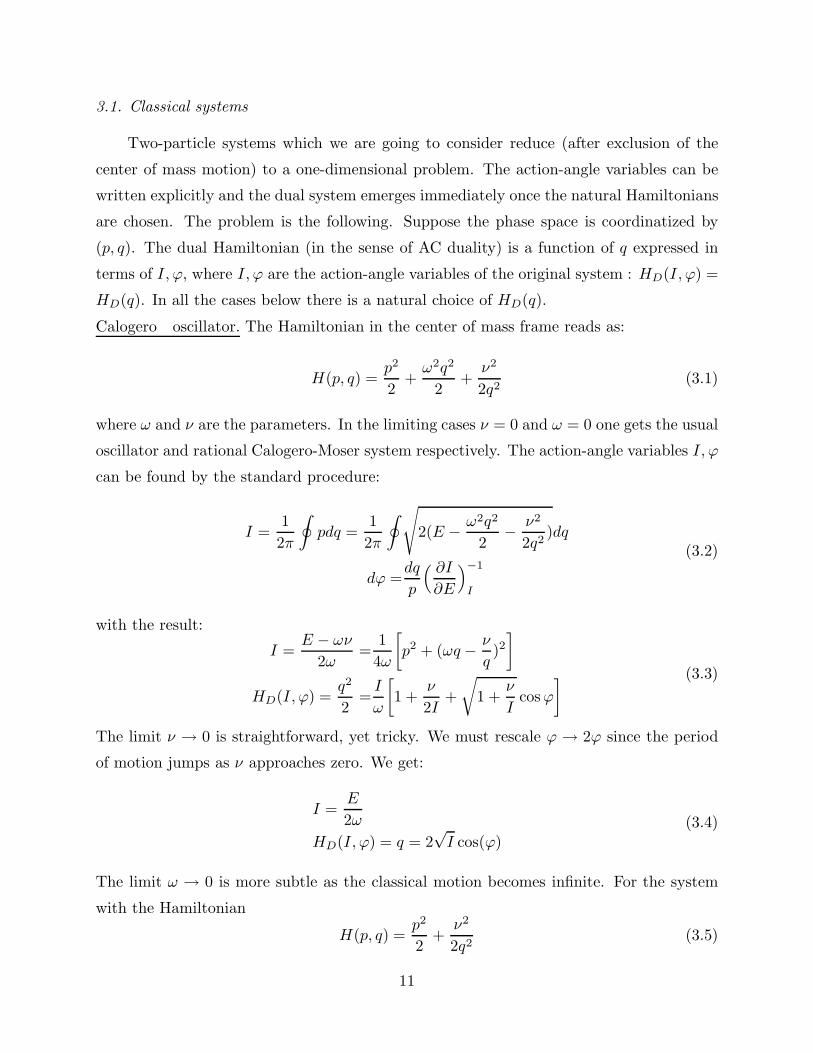
3.1. Classical systems

Two-particle systems which we are going to consider reduce (after exclusion of the

center of mass motion) to a one-dimensional problem. The action-angle variables can be

written explicitly and the dual system emerges immediately once the natural Hamiltonians

are chosen. The problem is the following. Suppose the phase space is coordinatized by

(p, q). The dual Hamiltonian (in the sense of AC duality) is a function of q expressed in

terms of I, ϕ, where I, ϕ are the action-angle variables of the original system : HD(I, ϕ) =

HD(q). In all the cases below there is a natural choice of HD(q).

Calogero oscillator. The Hamiltonian in the center of mass frame reads as:

H(p, q) =p2

2+ω2q2

2+

ν2

2q2(3.1)

where ω and ν are the parameters. In the limiting cases ν = 0 and ω = 0 one gets the usual

oscillator and rational Calogero-Moser system respectively. The action-angle variables I, ϕ

can be found by the standard procedure:

I =1

2π

∮pdq =

1

2π

∮ √

2(E − ω2q2

2− ν2

2q2)dq

dϕ =dq

p

( ∂I∂E

)−1

I

(3.2)

with the result:

I =E − ων

2ω=

1

4ω

[p2 + (ωq − ν

q)2

]

HD(I, ϕ) =q2

2=I

ω

[1 +

ν

2I+

√1 +

ν

Icosϕ

] (3.3)

The limit ν → 0 is straightforward, yet tricky. We must rescale ϕ → 2ϕ since the period

of motion jumps as ν approaches zero. We get:

I =E

2ω

HD(I, ϕ) = q = 2√I cos(ϕ)

(3.4)

The limit ω → 0 is more subtle as the classical motion becomes infinite. For the system

with the Hamiltonian

H(p, q) =p2

2+

ν2

2q2(3.5)

11

the action variable could be defined as the asymptotic value of the momentum: I =√

2E.

This choice gives rise to the evolution, linear in the “angle”-like variable,

ϕ =

√q2 − ν2

2E

HD(I, ϕ) =q2

2=ϕ2

2+

ν2

2I2

(3.6)

Sutherland model. The Hamiltonian is:

H(p, q) =1

2p2 +

ν2

2sin2(q). (3.7)

The action variable I can be chosen to be:

I =√

2E (3.8)

To prove that one might go to the coordinate t = cos(q) and compute the integral 12π

∮pdq

by residues. The angle variable ϕ can be determined from the condition dp∧dq = dI ∧dϕ.

We get:

dϕ =Idq√

I2 − 2ν2

sin2(q)

(3.9)

HD(I, ϕ) = cos(q) = cosϕ

√1 − 2ν2

I2(3.10)

Notice, that (3.10) coincides with the Hamiltonian of the rational Ruijsenaars model (see

below).

Elliptic Calogero − Moser system. The Hamiltonian is:

H(p, q) =p2

2+ ν2℘τ (q) (3.11)

Here p, q are complex, ℘τ (q) is the Weierstrass function on the elliptic curve Eτ :

℘τ (q) =1

q2+

∑

(m,n) ∈ ZZ2

(m,n) 6= (0, 0)

1

(q +mπ + nτπ)2− 1

(mπ + nτπ)2(3.12)

Let us introduce the Weierstrass notations: x = ℘τ (q), y = ℘τ (q)′. We have an equation

defining the curve Eτ :

y2 = 4x3 − g2(τ)x− g3(τ) = 43∏

i=1

(x− ei),3∑

i=1

ei = 0 (3.13)

12

The holomorphic differential dq on Eτ equals dq = dx/y. Introduce the variable e0 = E/ν2.

The action variable is one of the periods of the differential pdq2π

on the curve E = H(p, q) :

I =1

2π

∮

A

dq√

2(E − ν2℘τ (q)) =iν

2√

2π

∮

A

dx√x− e0√

(x− e1)(x− e2)(x− e3)(3.14)

The angle variable can be determined from the condition dp ∧ dq = dI ∧ dϕ:

dϕ =1

2iT (E)

dx√∏3i=0(x− ei)

(3.15)

where T (E) normalizes dϕ in such a way that the A period of dϕ is equal to 2π:

T (E) =1

4πi

∮

A

dx√∏3i=0(x− ei)

(3.16)

Thus:

2iT (E)dϕ =dx√

4∏3

i=0(x− ei)

ωdϕ =dt√

4∏3

i=1(t− ti)

(3.17)

where

ω = −2iT (E)√e01e02e03 =

1

2π

∮

A

dt√4

∏3i=1(t− ti)

t =1

x− e0+

1

3

3∑

i=1

1

e0iti =

1

3

3∑

j=1

eji

e0ie0j

eij = ei − ej

(3.18)

Introduce a meromorphic function on Eτ :

cnτ (z) =

√x− e1x− e3

(3.19)

where z has periods 2π and 2πτ . It is an elliptic analogue of the cosine (in fact, up to a

rescaling of z it coincides with the Jacobi elliptic cosine). Then we have:

HD(I, ϕ) = cnτ (z) = cnτE(ϕ)

√

1 − ν2e132E − ν2e3

(3.20)

13

where τE is the modular parameter of the relevant spectral curve v2 = 4∏3

i=1(t− ti):

τE =(∮

B

dt√4

∏3i=1(t− ti)

)/(∮

A

dt√4

∏3i=1(t− ti)

). (3.21)

For large I, 2E(I) ∼ I2

Elliptic Ruijsenaars model. The Hamiltonian is:

H(p, q) = cos(βp)√

1 − 2(βν)2℘τ (q). (3.22)

As the curve Eτ degenerates one flows down to the trigonometric (℘τ (q) → 1sin2(q)

) or

rational (℘τ (q) → 1q2 ) Ruijsenaars system. The spectral curve H(p, q) = E helps to define

the action variable I:

I =1

2π

∮

A

pdq, (3.23)

up to the transformations

I → n1ID + n2I +

2π

βn3

where n1, n2, n3 ∈ ZZ and (n1, n2) = 1. These transformations reflect the freedom in the

choice of the cycle A on the spectral curve. The appearence of n3 was used in [39]. We

can write an explicit formula for the quantity which is better defined:

∂I

∂E=

1

2√

2πβ2ν

∮

A

dx√∏3i=0(x− ei)

(3.24)

where now e0 = 1−E2

2(βν)2. Under A→ B transformation ∂I

∂Egets multiplied by τE , where τE

is defined as in (3.21) . Quite similarly to (3.17) we get:

dϕ =1

T (E)

dx√∏3i=0(x− ei)

(3.25)

with

T (E) =1

2π

∮

A

dx√∏3i=0(x− ei)

(3.26)

Finally, for HD given by (3.19) we get:

HD(I, ϕ) = cnτ (z) = cnτE(ϕ)

√

1 − 2(βν)2e13

E(I)2 − 1 − 2(βν)2e3

(3.27)

14

Asymptotically, for large I, E(I) ∼ cos(βI).

General elliptic model. In the general case one modifies the formula (3.13) in such a

way that the coefficients g2 and g3 are the sections of the line bundles O(4n) and O(6n)

respectively over B ≈ IP1. The elliptic curve Ez defined by the modified (3.13) degenerates

over the divisor of zeroes of its discriminant:

∆ = g32 − 27g2

3 (3.28)

which is a section of O(12n). The latter has generically 12n zeroes. To make the total

space of fibration isomorphic to the K3 surface (compact simply-connected symplectic

surface) we need 24 singular fibers, i.e. n = 2. The Hamiltonian of the integrable system

we consider is any function on B. It gives rise to a meromorphic vector field on M , which

linearizes along the elliptic fibers. The symplectic form is given by:

ω =dx ∧ dz

y(3.29)

where z is the projective coordinate on B. Under change of the variables: z = 1z, y = − y

z6 ,

x = xz4 the form (3.29) goes over to dx∧dz

yand the equation (3.13) is mapped to

y2 = 4x3 − g2(z)x− g3(z)

where the polynomials gk are defined through the relation:

gk(z) = z4kgk(1/z).

Over a simply connected region U ⊂ IP1\∆−1(0) one can trivialize the bundle of the

first homologies IH1(Ez,ZZ), in particular to make a well-defined choice of the A-cycle of

the elliptic fibre. The local action variable I = I(z) is defined over U by the equation:

dI(z)

dz= T (z) =

1

2π

∮

A

dx

y(3.30)

where the integral is taken over a chosen A-cycle. The fibration of IH1(Ez,ZZ) over

B\∆−1(0) is non-trivial and there is no global monodromy invariant choice of A-cycles.

So the action variable is defined by (3.30) only locally. The monodromies around the de-

generate fibers corresponding to various singularities has been worked out by Kodaira and

their physical interpretation can be found in [40]. For generic polynomials g2(z), g3(z) the

singularities are of the type A1.

15

The angle variable dual to I(z) is nothing but the linear coordinate on the Jacobian of

the fiber elliptic curve (3.13). In particular it is periodic with the periods 2π and 2πτ(z).

It is to be found from the relation:

dϕ =1

T (z)

dx

y. (3.31)

We can get a dual system by treating x as the Hamiltonian. Since x is not a mero-

morphic function on K3 (it changes under the z → 1z

transformation) this is only possible

if we delete the elliptic fiber E∞.

Let us see what will be the action-angle variables. First of all, generically the fiber Cx

over x ∈ IP1 is an incomplete hyperelliptic curve of genus 5. The holomorphic differentials

on this curve are:

ωk =zkdz√

4x3 − g2(z)x− g3(z), k = 0, . . .4

The action variable ID = ID(x) obeys the equation:

dID

dx= TD(x) =

1

2π

∮

L

dz

y(3.32)

where L is a one-cycle in IH1(Cx,ZZ). Here we face AA duality in its extreme form:

the freedom to choose L is much bigger then in the case of original system, since the

corresponding duality group is Sp10(ZZ). We can partially integrate (3.32) to get

ID =1

2π

∮

L

ϕT (z)dz (3.33)

where

x =1

T (z)2℘ (ϕ; τ(z))

The angle variable is one of the linear coordinates on the Jacobian variety of Cx, which is

5 dimensional abelian variety:

dϕD =1

TD(x)

dz

y

The embedding of the Liouville tori into the abelian varieties of higher rank originating

from hyperelliptic curves is a well-known phenomenon in the theory of integrable systems,

going back to the original work of S. Novikov and A. Veselov [41].

16

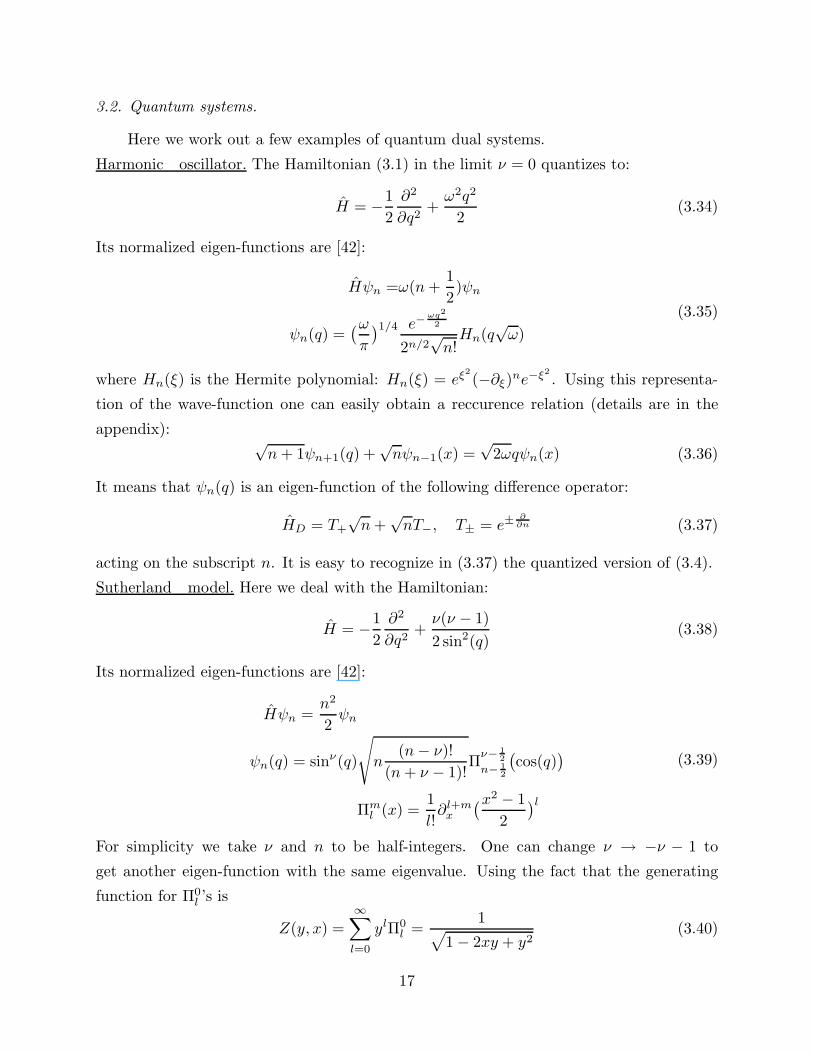
3.2. Quantum systems.

Here we work out a few examples of quantum dual systems.

Harmonic oscillator. The Hamiltonian (3.1) in the limit ν = 0 quantizes to:

H = −1

2

∂2

∂q2+ω2q2

2(3.34)

Its normalized eigen-functions are [42]:

Hψn =ω(n+1

2)ψn

ψn(q) =(ωπ

)1/4 e−ωq2

2

2n/2√n!Hn(q

√ω)

(3.35)

where Hn(ξ) is the Hermite polynomial: Hn(ξ) = eξ2

(−∂ξ)ne−ξ2

. Using this representa-

tion of the wave-function one can easily obtain a reccurence relation (details are in the

appendix): √n+ 1ψn+1(q) +

√nψn−1(x) =

√2ωqψn(x) (3.36)

It means that ψn(q) is an eigen-function of the following difference operator:

HD = T+

√n+

√nT−, T± = e±

∂∂n (3.37)

acting on the subscript n. It is easy to recognize in (3.37) the quantized version of (3.4).

Sutherland model. Here we deal with the Hamiltonian:

H = −1

2

∂2

∂q2+ν(ν − 1)

2 sin2(q)(3.38)

Its normalized eigen-functions are [42]:

Hψn =n2

2ψn

ψn(q) = sinν(q)

√

n(n− ν)!

(n+ ν − 1)!Π

ν− 12

n− 12

(cos(q)

)

Πml (x) =

1

l!∂l+m

x

(x2 − 1

2

)l

(3.39)

For simplicity we take ν and n to be half-integers. One can change ν → −ν − 1 to

get another eigen-function with the same eigenvalue. Using the fact that the generating

function for Π0l ’s is

Z(y, x) =∞∑

l=0

ylΠ0l =

1√1 − 2xy + y2

(3.40)

17

one derives the recurrence relations (details are in the appendix):

xΠml =

l + 1 −m

2l + 1Πm

l+1 +l +m

2l + 1Πm

l−1

cos(q)ψn =1

2

(√1 − ν(ν − 1)

n(n+ 1)ψn+1 +

√1 − ν(ν − 1)

n(n− 1)ψn−1

) (3.41)

that is ψn is an eigen-function of the finite-difference operator acting on the n subscript:

HDψ(q) = cos(q)ψ(q)

HD = T+

√

1 − ν(ν − 1)

n(n− 1)+

√

1 − ν(ν − 1)

n(n− 1)T−

(3.42)

which is a quantum version of (3.10).

Moral of the story. The moral of the previous discussion is that the polynomial de-

pendence on momenta of the hamiltonian is traded with the rational potential of the

dual system. The trigonometric potential is mapped to the trigonometric (= relativis-

tic) dependence on momenta of dual system. The elliptic potential gives rise to elliptic

(=“double-relativistic” ) dependence on momentum of the dual system Hamiltonian. When

the system with trigonometric dependence on momentum is quantized its Hamiltonian be-

comes a finite- difference operator. The wave-functions become the functions of the discrete

variables. The origin of this is in the Bohr-Sommerfeld quantization condition. Indeed,

since the trigonometric dependence of momenta implies that the leaves of the polarization

are compact and moreover non-simply connected the covariantly constant sections of the

prequantization connection along the polarization fiber generically seases to exist. It is

only for special “quantized” values of the action variables that the section exists. In the

elliptic case the quantum dual Hamiltonian is going to be a difference operator of the infi-

nite order. The self-dual elliptic many-body system is still to be constructed. It seems that

to achieve this goal one needs a notion of the Heisenberg double for the central extension

of the two dimensional current group [43].

Example of the prepotential. To illustrate the meaning of the AA duality we look at

the two-body system, relevant for the SU(2) N = 2 supersymmetric gauge theory [16]:

H =p2

2+ Λ2 cos(q) (3.43)

with Λ2 being a complex number - the coupling constant of a two-body problem and at the

same time a dynamically generated scale of the gauge theory. The action variable is given

18

by one of the periods of the differential pdq. Let us introduce more notations: x = cos(q),

y = p sin(q)√−2Λ

, u = HΛ2 . Then the spectral curve, associated to the system (3.43) which is also

a level set of the Hamiltonian can be written as follows:

y2 = (x− u)(x2 − 1) (3.44)

which is exactly Seiberg-Witten curve [12] as it was first observed in [16]. The periods are:

I =

∫ 1

−1

√x− u

x2 − 1dx,

ID =

∫ u

1

√x− u

x2 − 1dx

(3.45)

They obey Picard-Fuchs equation:

(d2

du2+

1

4(u2 − 1)

) (IID

)= 0

which can be used to write down an asymptotic expansion of the action variable near

u = ∞ or u = ±1 as well as that of prepotential (2.7). The AA duality is manifested

in the fact that near u = ∞ (which corresponds to the high energy scattering in the

two-body problem and also a perturbative regime of SU(2) gauge theory) the appropriate

action variable is I (it experiences a monodromy I → −I as u goes around ∞), while near

u = 1 (which corresponds to the dynamics of the two-body system near the top of the

potential and to the strongly coupled SU(2) gauge theory) the appropriate variable is ID

(which corresponds to a weakly coupled magnetic U(1) gauge theory and is actually well

defined near u = 1 point) [12]. The monodromy invariant combination of the periods [44]:

IID − 2F = u (3.46)

(whose origin is in the periods of Calabi-Yau manifolds on the one hand and in the proper-

ties of anomaly in theory on the other) can be chosen as a global coordinate on the space

of integrals of motion B. At u→ ∞ the prepotential has an expansion of the form:

F ∼ 1

2u log u+ . . . ∼ I2 log I +

∑

n

fn

nI2−4n

19

3.3. Appendix.

To derive the recurrence relation for the oscillator wave-functions we use the creation

operator representation: ψn = 1√2n

(−∂ξ + ξ)ψn. Applying this relation twice and using

the fact that ψn is an eigen-function of H one arrives at (3.36). For the Sutherland model

we use two obvious relations:

(x− y)∂xZ = y∂yZ (3.47)

(1 − 2xy + y2)∂yZ = (x− y)Z (3.48)

Next, (3.47) implies:

(y∂y −m)∂mx Z = (x− y)∂m+1

x Z (3.49)

and (3.48) yields:

((1 − 2xy + y2)∂y + y − x

)∂m

x Z = m(1 + 2y∂y)∂m−1x Z (3.50)

Combination of those two gives rise to (3.41).

20

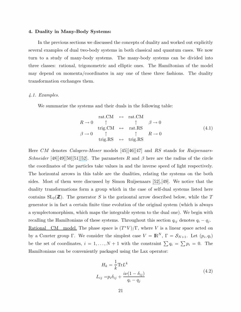
4. Duality in Many-Body Systems:

In the previous sections we discussed the concepts of duality and worked out explicitly

several examples of dual two-body systems in both classical and quantum cases. We now

turn to a study of many-body systems. The many-body systems can be divided into

three classes: rational, trigonometric and elliptic ones. The Hamiltonian of the model

may depend on momenta/coordinates in any one of these three fashions. The duality

transformation exchanges them.

4.1. Examples.

We summarize the systems and their duals in the following table:

rat.CM ↔ rat.CMR→ 0 ↑ ↑ β → 0

trig.CM ↔ rat.RSβ → 0 ↑ ↑ R→ 0

trig.RS ↔ trig.RS

(4.1)

Here CM denotes Calogero-Moser models [45][46][47] and RS stands for Ruijsenaars-

Schneider [48][49][50][51][52]. The parameters R and β here are the radius of the circle

the coordinates of the particles take values in and the inverse speed of light respectively.

The horizontal arrows in this table are the dualities, relating the systems on the both

sides. Most of them were discussed by Simon Ruijsenaars [52],[49]. We notice that the

duality transformations form a group which in the case of self-dual systems listed here

contains SL2(ZZ). The generator S is the gorizontal arrow described below, while the T

generator is in fact a certain finite time evolution of the original system (which is always

a symplectomorphism, which maps the integrable system to the dual one). We begin with

recalling the Hamiltonians of these systems. Throughout this section qij denotes qi − qj .

Rational CM model. The phase space is (T ∗V )/Γ, where V is a linear space acted on

by a Coxeter group Γ. We consider the simplest case V = IRN , Γ = SN+1. Let (pi, qi)

be the set of coordinates, i = 1, . . . , N + 1 with the constraint∑qi =

∑pi = 0. The

Hamiltonians can be conveniently packaged using the Lax operator:

Hk =1

kTrLk

Lij =piδij +iν(1 − δij)

qi − qj

(4.2)

21

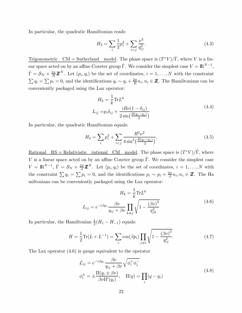
In particular, the quadratic Hamiltonian reads:

H2 =∑

i

1

2p2

i +∑

i<j

ν2

q2ij. (4.3)

Trigonometric CM = Sutherland model. The phase space is (T ∗V )/Γ, where V is a lin-

ear space acted on by an affine Coxeter group Γ. We consider the simplest case V = IRN−1,

Γ = SN × 2πR ZZ

N . Let (pi, qi) be the set of coordinates, i = 1, . . . , N with the constraint∑qi =

∑pi = 0, and the identifications qi ∼ qi + 2π

R ni, ni ∈ ZZ. The Hamiltonians can be

conveniently packaged using the Lax operator:

Hk =1

kTrLk

Lij =piδij +iRν(1 − δij)

2 sin(R(qi−qj)

2

)(4.4)

In particular, the quadratic Hamiltonian equals:

H2 =∑

i

p2i +

∑

i<j

R2ν2

4 sin2(R(qi−qj)

2

) . (4.5)

Rational RS = Relativistic rational CM model. The phase space is (T ∗V )/Γ, where

V is a linear space acted on by an affine Coxeter group Γ. We consider the simplest case

V = IRN−1, Γ = SN × 2πβ

ZZN . Let (pi, qi) be the set of coordinates, i = 1, . . . , N with

the constraint∑qi =

∑pi = 0, and the identifications pi ∼ pi + 2π

β ni, ni ∈ ZZ. The Ha

miltonians can be conveniently packaged using the Lax operator:

Hk =1

kTrLk

Lij = e−iβpiβν

qij + βν

∏

k 6=j

√

1 − (βν)2

q2jk

(4.6)

In particular, the Hamiltonian 12(H1 −H−1) equals:

H =1

2Tr(L+ L−1) =

∑

i

cos(βpi)∏

j 6=i

√

1 − (βν)2

q2ij. (4.7)

The Lax operator (4.6) is gauge equivalent to the operator

Lij = e−iβpiβν

qij + βν

√φ+

i φ−j

φ±i = ±Π(qi ± βν)

βνΠ′(qi), Π(q) =

∏

i

(q − qi)(4.8)

22

In the limit β → 0 both L,L of (4.6),(4.8) behave as Id−iβ ( Lax operator in (4.2) )+o(β).

Trigonometric RS = Relativistic Sutherland model. The phase space is (T ∗V )/ΓE ,

where V is a linear space acted on by a double affine Coxeter group ΓE , E being an

elliptic curve. We consider the simplest case V = IRN−1, Γ = SN ×(

2πβ

ZZN ⊕ 2π

RZZ

N). Let

(pi, qi) be the set of coordinates, i = 1, . . . , N with the constraint∑qi =

∑pi = 0, and

the identifications pi ∼ pi + 2πβ ni, qi ∼ qi + 2π

R mi, ni, mi ∈ ZZ. The Hamiltonians

can be conveniently packaged using the Lax operator:

Hk =1

kTrLk

Lij = e−iβpi

sin(

Rβν2

)

sin(

R2(qij + βν)

)∏

k 6=j

√√√√√1 −sin2

(Rβν

2

)

sin2(

Rqjk

2

)(4.9)

In particular, the Hamiltonian 12(H1 −H−1) equals:

H =1

2Tr(L+ L−1) =

∑

i

cos(βpi)∏

j 6=i

√√√√1 − sin2(Rβν)

sin2(R(qij)

2

) . (4.10)

The Lax operator (4.6) is gauge equivalent to the operator

Lij = e−iβpi

sin(

NRβν2

)

Nsin(

R2 (qij + βν)

)√

Φ+i Φ−

j

Φ±i = ± NR

2sin(

NRβν2

) P (qi ± βν)

P ′(qi), P (q) =

N∏

i=1

sin

(R

2(q − qi)

) (4.11)

In the limit R → 0, with β fixed the expressions (4.9),(4.10),(4.11) naturally go over to

(4.6), (4.7), (4.8) respectively. In the limit β → 0, R fixed both L,L behave as Id−iβ( Lax

operator in (4.4) ) + o(β).

4.2. Explanations: Hamiltonian and/or Poisson reduction

Suppose we are given a symplectic manifold (X,ωX) with the Hamiltonian action of

a Lie group G with equivariant moment map µ : X → g∗. The symplectic quotient of X

with respect to G is the symplectic manifold M , denoted as X//G and defined as:

M = µ−1(0)/G

23

Its symplectic form ωM is defined through the relation:

p∗ωM = i∗ωX

where p : µ−1(0) →M is the projection and i : µ−1(0) → X is the inclusion.

Let us assume that an integrable Hamiltonian system is defined on X . Let K =

K1, . . . , Kx, x = 12dimX denote the set of its integrals of motion. Suppose that this

system is equivariant with respect to the action of G. This is equivalent to the statement,

that Ki and µa form a closed algebra K with respect to the Poisson brackets. Let us

assume that on the zero level of the moment map µ the center Z(K) of the algebra K is

sufficiently big, i.e. the dimension of its spectrum equals half the dimension of M . Then

the integrable system on X descends to the integrable system on M , K being replaced by

Z(K).

Now let us impose one further restriction. Suppose that X possesses another G-

equivariant integrable Hamiltonian system, with integrals Q = Q1, . . . , Qx, which is

dual to the system K (algebraically it means that K and Q generate all functions on X).

We also assume that Q descends to M .

On the original manifold X the evolution of the system K looks non-trivially in the

action-angle variables for the system Q and vice versa. The same is true for the reduced

systems. The advantage of the consideration of X is that the systems on X can be much

simpler then those on M . In the following sections we shall consider various examples of

this situation.

The similar statements hold in the case of Poisson manifolds, the relevant reduction

being the Poisson one (one first takes a quotient with respect to the group and then picks

out a symplectic leaf). We leave the details to the interested readers.

Now we proceed to the explicit constructions. We will discuss the models introduced

in the previous section on case-by-case basis and show how the reduction which yields

these systems also explains the dualities between different systems.

Rational CM model. This model can be obtained as a result of Hamiltonian reduction

applied to T ∗g×O [53] for g = su(N), O = CIPN−1. The symplectic form on this manifold

is the sum of Liouville form on T ∗g and −Nν× Fubini-Study form on O. Let (e1 : . . . : eN )

be the homogeneous coordinates on O. The group G = SU(N) acts on T ∗g via conjugation

and on O in a standard way (O = G/H, H = S(U(N − 1) × U(1))). Then the moment

map for the action of G on T ∗g ×O is

µ = ad∗Q(P ) − J Jij = ν(Nδij − eie∗j ) (4.12)

24

where Q ∈ g, P ∈ g∗. Now we choose two sets of Hamiltonians:

Hk =1

kTrP k and HD

k =1

kTrQk (4.13)

If we identify g∗ and g with the help of Tr then the equation µ = 0 has the form:

[P,Q] = J (4.14)

which is obviously preserved by the involution: P → Q,Q → −P . So we are guaranteed

to get a self-dual system. Now we have to find suitable coordinates and action variables.

Let us choose the gauge (remember that we have to mod out (4.14) by the action of G):

Q = diag(q1, . . . , qN ) (4.15)

This gauge is preserved by the action of the maximal torus T = U(1)N−1 which turns out

to be sufficient to set all ei to be equal: ei = 1 [54]. Then the equation (4.14) fixes P

which turns out to be nothing but L in (4.2). As it is obvious that the reduced symplectic

form equals∑

i dpi ∧dqi (with the constraint∑qi =

∑pi = 0) one concludes that qi’s are

the action variables for the system generated by HDk ’s. Therefore eigenvalues of P are the

action variables for the flows generated by Hk’s. We therefore proved the following

Statement. Consider the map:

σ : (pi, qi) → (ξi,−ηi) (4.16)

where ηi’s are the eigenvalues of L ≡ P and ξi are the diagonal entries of Q in the

eigenbasis of P . It is an involution.

Let us go back to the systems (4.13). The moment map equation (4.14) is obviously

preserved by the transformations of the form

(P,Q) 7→ (aP + bQ, cP + dQ) ad− bc = 1 (4.17)

which form SL2(IR) group. The transformed Hamiltonians

g ·Hk =1

kTr(aP + bQ)k

are easy to express through the original Hamiltonians (4.13) in the coordinates (pi, qi):

g ·Hk(pi, qi)|ν = Hk(api + bqi, qi)|aν

25

Let us restrict our attention to the SL2(ZZ) subgroup of the group (4.17). It is generated

by the transformations

S =

(0 −11 0

)T =

(1 10 1

)(4.18)

It is clear that S coincides with the involution leading to (4.16) while T is the unit time

evolution with respect to the Hamiltonian HD2 .

Trigonometric CM, Rational RS. The trigonometric CM system can be obtained as

Hamiltonian reduction applied to either T ∗G × O [53] or T ∗g × O [55] where g is the

central extension of the loop algebra. In the latter case one has to specify the action of

the gauge group LG on the orbit O. The correct choice is the most natural one: since the

orbit is finite-dimensional, the only sensible way the loop group can act on it is through

the evaluation at some point. The elements of T ∗g of our interest are the pairs:

P (x), k∂x +Q(x) (4.19)

where k is a fixed number, P (x) is a g-valued function on a circle S1 and Q(x) is a gauge

field on a circle. The phase space is acted on by the gauge group:

P (x) 7→ g(x)−1P (x)g(x), Q(x) 7→ g(x)−1Q(x)g(x) + kg−1(x)∂xg(x) (4.20)

The moment equation has the form:

k∂xP + [Q,P ] = Jδ(x) (4.21)

where J is the one from (4.12). The number k can be rescaled by the choice of the radius

of a circle S1. Instead we choose the circle of unit radius and keep k. To solve the equation

(4.21) we fix a gauge (4.20). We can either decide that Q is a constant diagonal matrix

Q = diag(q1, . . . , qN )

and then the solution for P (x) will produce the Lax operator (4.4) of the Sutherland model

with R = 2πk [55],[56].

It is quite amusing that the same reduction yields the rational RS model as well. In

order to see that choose the gauge

P (x) = diag (p1 (x) , . . . , pN (x)) (4.22)

26

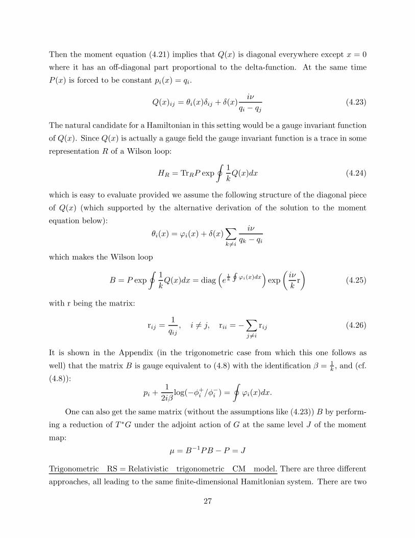
Then the moment equation (4.21) implies that Q(x) is diagonal everywhere except x = 0

where it has an off-diagonal part proportional to the delta-function. At the same time

P (x) is forced to be constant pi(x) = qi.

Q(x)ij = θi(x)δij + δ(x)iν

qi − qj(4.23)

The natural candidate for a Hamiltonian in this setting would be a gauge invariant function

of Q(x). Since Q(x) is actually a gauge field the gauge invariant function is a trace in some

representation R of a Wilson loop:

HR = TrRP exp

∮1

kQ(x)dx (4.24)

which is easy to evaluate provided we assume the following structure of the diagonal piece

of Q(x) (which supported by the alternative derivation of the solution to the moment

equation below):

θi(x) = ϕi(x) + δ(x)∑

k 6=i

iν

qk − qi

which makes the Wilson loop

B = P exp

∮1

kQ(x)dx = diag

(e

1k

∮ϕi(x)dx

)exp

(iν

kr

)(4.25)

with r being the matrix:

rij =1

qij, i 6= j, rii = −

∑

j 6=i

rij (4.26)

It is shown in the Appendix (in the trigonometric case from which this one follows as

well) that the matrix B is gauge equivalent to (4.8) with the identification β = 1k , and (cf.

(4.8)):

pi +1

2iβlog(−φ+

i /φ−i ) =

∮ϕi(x)dx.

One can also get the same matrix (without the assumptions like (4.23)) B by perform-

ing a reduction of T ∗G under the adjoint action of G at the same level J of the moment

map:

µ = B−1PB − P = J

Trigonometric RS = Relativistic trigonometric CM model. There are three different

approaches, all leading to the same finite-dimensional Hamitlonian system. There are two

27

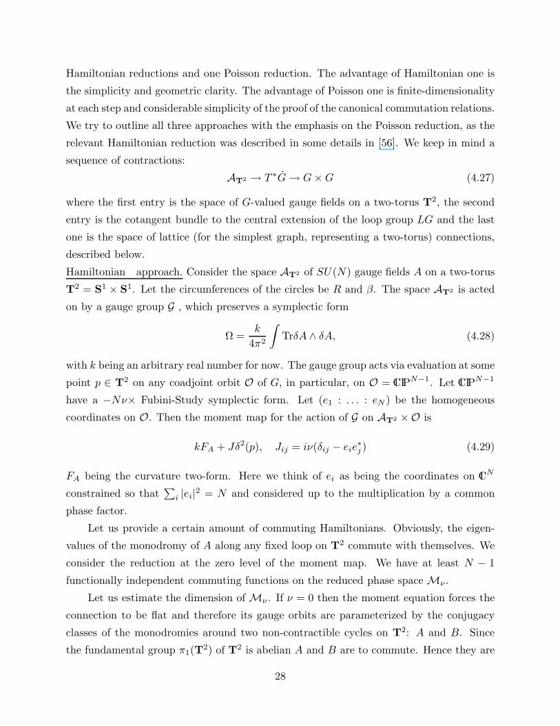
Hamiltonian reductions and one Poisson reduction. The advantage of Hamiltonian one is

the simplicity and geometric clarity. The advantage of Poisson one is finite-dimensionality

at each step and considerable simplicity of the proof of the canonical commutation relations.

We try to outline all three approaches with the emphasis on the Poisson reduction, as the

relevant Hamiltonian reduction was described in some details in [56]. We keep in mind a

sequence of contractions:

AT2 → T ∗G→ G×G (4.27)

where the first entry is the space of G-valued gauge fields on a two-torus T2, the second

entry is the cotangent bundle to the central extension of the loop group LG and the last

one is the space of lattice (for the simplest graph, representing a two-torus) connections,

described below.

Hamiltonian approach. Consider the space AT2 of SU(N) gauge fields A on a two-torus

T2 = S1 × S1. Let the circumferences of the circles be R and β. The space AT2 is acted

on by a gauge group G , which preserves a symplectic form

Ω =k

4π2

∫TrδA ∧ δA, (4.28)

with k being an arbitrary real number for now. The gauge group acts via evaluation at some

point p ∈ T2 on any coadjoint orbit O of G, in particular, on O = CIPN−1. Let CIPN−1

have a −Nν× Fubini-Study symplectic form. Let (e1 : . . . : eN ) be the homogeneous

coordinates on O. Then the moment map for the action of G on AT2 ×O is

kFA + Jδ2(p), Jij = iν(δij − eie∗j ) (4.29)

FA being the curvature two-form. Here we think of ei as being the coordinates on CN

constrained so that∑

i |ei|2 = N and considered up to the multiplication by a common

phase factor.

Let us provide a certain amount of commuting Hamiltonians. Obviously, the eigen-

values of the monodromy of A along any fixed loop on T2 commute with themselves. We

consider the reduction at the zero level of the moment map. We have at least N − 1

functionally independent commuting functions on the reduced phase space Mν .

Let us estimate the dimension of Mν . If ν = 0 then the moment equation forces the

connection to be flat and therefore its gauge orbits are parameterized by the conjugacy

classes of the monodromies around two non-contractible cycles on T2: A and B. Since

the fundamental group π1(T2) of T2 is abelian A and B are to commute. Hence they are

28

simultaneously diagonalizable, which makes M0 a 2(N − 1) dimensional manifold. Notice

that the generic point on the quotient space has a non-trivial stabilizer, isomorphic to the

maximal torus T of SU(N). Now, in the presence of O the moment equation implies that

the connection A is flat outside of p and has a non-trivial monodromy around p. Thus:

ABA−1B−1 = exp(RβJ) (4.30)

(the factor Rβ comes from the normalization of the delta-function in (4.29)). If we diago-

nalize A, then B is uniquely reconstructed up to the right multiplication by the elements

of T . The potential degrees of freedom in J are ”eaten” up by the former stabilizer T of a

flat connection: if we conjugate both A and B by an element t ∈ T then J gets conjugated.

Now, it is important that O has dimension 2(N−1). The reduction of O with respect to T

consists of a point and does not contribute to the dimension of Mν . Thereby we expect to

get an integrable system. Without doing any computations we already know that we get a

pair of dual systems. Indeed, we may choose as the set of coordinates the eigen-values of A

or the eigen-values of B. The logarithms of the eigen-values of B are the action variables

for the system generated by TrBk, and vice versa.

The two-dimensional picture has the advantage that the geometry of the problem

suggests the SL2(ZZ)-like duality. Consider the operations S and T realized as:

S : (A,B) 7→ (ABA−1, A−1); T : (A,B) 7→ (A,BA) (4.31)

which correspond to the freedom of choice of generators in the fundamental group of a two-

torus. Notice that both S and T preserve the commutator ABA−1B−1 and commute with

the action of the gauge group. The group Γ generated by S and T (it is a subrogup of the

group OutFree(2) of the outer authomorphismes of the free group with two generators)

seems to be larger then SL2(ZZ). However in the limit β,R → 0 it contracts to SL2(ZZ) in

a sense that we get the transformations (4.18) by expanding

A = 1 + βP + . . . , B = 1 +RQ+ . . .

for R, β → 0.

The disadvantage of the two-dimensional picture us the necessity to keep too many

redundant degrees of freedom. The first of the contractions (4.27) actually allows to replace

the space of two dimensional gauge fields by the cotangent space to the (central extension

of) loop group:

T ∗G = (g(x), k∂x + P (x))

29

which is a “deformation” of the phase space of the previous example (Q(x) got promoted

to a group-valued field). The relation to the two dimensional construction is the following.

Choose a non-contractible circle S1 on the two-torus which does not pass through the

marked point p. Let x, y be the coordinates on the torus and y = 0 is the equation of the

S1. The periodicity of x is β and that of y is R. Then

P (x) = Ax(x, 0), g(x) = P exp

∫ R

0

Ay(x, y)dy.

The gauge transformations on S1 transform on (g(x), P (x)) is a way, similar to (4.20).

The moment map equation (4.29) goes over to the moment map equation [56]:

kg−1∂xg + g−1Pg − P = Jδ(x), (4.32)

with k = 1Rβ

. The solution of this equation in the gauge P = diag(q1, . . . , qN ) leads to the

Lax operator A = g(0) of the form (4.11) with R, β exchanged [56]. On the other hand, if

we follow (4.22) and diagonalize g(x):

g(x) = diag(z1 = eiRq1 , . . . , zN = eiRqN

)(4.33)

then a similar calculation leads to the Lax operator

B = P exp

∮1

kP (x)dx = diag(eiθi) exp iRβνr

with

rij =1

1 − eiRqji, i 6= j; rii = −

∑

j 6=i

rij

thereby establishing the duality A↔ B explicitly.

Poisson description. Here we introduce a set of commuting functions on the space of

graph connection on a graph, corresponding to a moduli space of flat connections on a

torus with one hole and describe the flow generated by this set. Being reduced to a

particular symplectic leaf of the moduli space of flat connections on the torus , this set

of functions turns out to be a full set of commuting Hamiltonians. We introduce another

full set of commuting variables and write down the Hamiltonians taking the latter set as

a set of coordinates thus recovering the Ruijsenaars integrable system. Consider a graph,

consisting of two edges and one vertex with the fat graph structure corresponding to a

punctured torus [57]. The space of graph connections AL for such graph is just a product

30

of two copies of the group G: AL = G × G = (A,B)|A,B ∈ G, where A and B are

assigned to the edges of the graph. For a choice of ciliation on AL the Poisson bracket on

AL is given by the relations, following from the general rules [57].

A⊗,A = raA⊗ A+A⊗ Ara − 2(A⊗ 1)ra(1 ⊗ A)

B⊗,B = raB ⊗B +B ⊗Bra − 2(B ⊗ 1)ra(1 ⊗B)

A⊗,B = r(A⊗B) +A⊗Br + (1 ⊗B)r21(A⊗ 1) − (A⊗ 1)r(1 ⊗B),

(4.34)

where ra = 12(r − r21).

Now let us restrict ourselves to the case G = SLN and the standard r-matrix:

r =∑

α>0

Eα ⊗ E−α +1

2

∑

i

Hi ⊗Hi, ra =1

2

∑

α>0

Eα ∧ E−α (4.35)

In this case one can easily derive the following commutaion relations

TrAn, A = 0 TrBn, B = 0 (4.36)

TrAn, B = n(An)0 TrBn, A = nA(Bn)0 (4.37)

where (X)0 denotes the traceless part of the matrix X . Therefore, the functions TrBn for

n = 1 . . .N − 1 considered as Hamiltonians generate commuting flows on AL.

B (t1, . . . , tN−1) = B (0, . . . , 0)

A (t1, . . . , tN−1) = A (0, . . . , 0) e

(t1B+···+tN−1BN−1

)0

(4.38)

As it was shown in [57] the lattice gauge group GL acts on GL in a Poisson way, and the

quotient Poisson manifold coincides with the moduli space M of smooth flat connection on

the Riemann surface, corresponding to the fat graph L. In our case the group GL is G itself

(for the graph has just one vertex) which acts on A and B by simultaneous conjugation.

g : (A,B) 7→ (gAg−1, gBg−1). (4.39)

The functions TrAk and TrBk are invariant under this action, and therefore their

pull-downs on the moduli space M generate commuting flows there, which trajectories are

just projections of (4.38).

However the moduli space M in our case is a Poisson manifold with degenerate Poisson

bracket. The Casimir functions of this Poisson structure are the functions of conjugacy

31

classes of monodromies around holes and constant value levels of such functions are just

the symplectic leaves of M. In our case such Casimir functions are Tr(ABA−1B−1

)k,

pulled down to M.

Different symplectic leaves have different dimensions and the lowest dimension of them

is 2(N − 1). These leaves correspond to the monodromy around the hole conjugated to a

matrix

e−iRβν Id + P,

rkP ≤ 1, ν is a numerical constant from the previous section parameterizing the set of

symplectic leaves of lowest dimension. Let t = e−iRβν . On the leaf Mν the family of

functions TrAk, k = 1, . . . , N − 1 forms a full set of Poisson-commuting variables.

Introduce local coordinates on these symplectic leaves in the following way. Let

z1 = eiRq1 , . . . , zN = eiRqN be the eigenvalues of the operator A and µ1, . . . , µN are

the corresponding diagonal matrix elements of B (in the basis, diagonalizing A). One can

check that in this basis

Bij =

√µiµj

(1 − t)

zi/zj − t. (4.40)

The functions zi and µj are well-defined locally on the symplectic leaf Mν . Their Poisson

brackets are equal to:

zi, zj = 0

µi, µj = µiµj(zi + zj)

(zi/zj − t)(zj/zi − t)(zi − zj)i 6= j

zi, µj = ziµjδi,j .

(4.41)

To define the variables, canonically conjugated to zi we can just multiply µi by factors

independent on µi. For example one can take:

si = µitN−1

2

∏

k,k 6=i

√(zk − zi)(zi − zk)

(zk − tzi)(zi − tzk)(4.42)

One can check, that these new variables si have the Poisson brackets

si, sj = 0 zi, sj = zisjδi,j . (4.43)

Substituting this back to the formula (4.40) we get:

Bij =1 − t

zi/zj − t

(Φ+

i Φ−i Φ+

j Φ−j

)1/4(4.44)

32

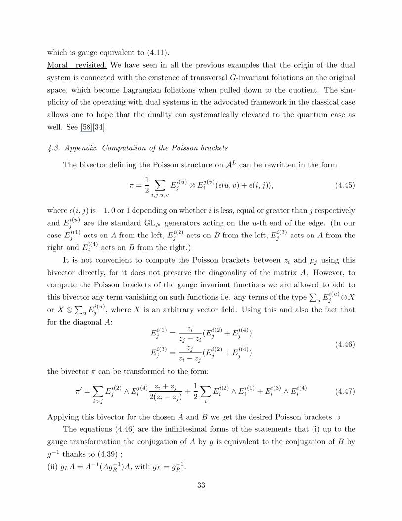
which is gauge equivalent to (4.11).

Moral revisited. We have seen in all the previous examples that the origin of the dual

system is connected with the existence of transversal G-invariant foliations on the original

space, which become Lagrangian foliations when pulled down to the quotient. The sim-

plicity of the operating with dual systems in the advocated framework in the classical case

allows one to hope that the duality can systematically elevated to the quantum case as

well. See [58][34].

4.3. Appendix. Computation of the Poisson brackets

The bivector defining the Poisson structure on AL can be rewritten in the form

π =1

2

∑

i,j,u,v

Ei(u)j ⊗ E

j(v)i (ǫ(u, v) + ǫ(i, j)), (4.45)

where ǫ(i, j) is −1, 0 or 1 depending on whether i is less, equal or greater than j respectively

and Ei(u)j are the standard GLN generators acting on the u-th end of the edge. (In our

case Ei(1)j acts on A from the left, E

i(2)j acts on B from the left, E

i(3)j acts on A from the

right and Ei(4)j acts on B from the right.)

It is not convenient to compute the Poisson brackets between zi and µj using this

bivector directly, for it does not preserve the diagonality of the matrix A. However, to

compute the Poisson brackets of the gauge invariant functions we are allowed to add to

this bivector any term vanishing on such functions i.e. any terms of the type∑

uEi(u)j ⊗X

or X ⊗ ∑uE

i(u)j , where X is an arbitrary vector field. Using this and also the fact that

for the diagonal A:

Ei(1)j =

zi

zj − zi(E

i(2)j +E

i(4)j )

Ei(3)j =

zj

zi − zj(E

i(2)j +E

i(4)j )

(4.46)

the bivector π can be transformed to the form:

π′ =∑

i>j

Ei(2)j ∧Ej(4)

i

zi + zj

2(zi − zj)+

1

2

∑

i

Ei(2)i ∧Ei(1)

i +Ei(3)i ∧Ei(4)

i (4.47)

Applying this bivector for the chosen A and B we get the desired Poisson brackets.

The equations (4.46) are the infinitesimal forms of the statements that (i) up to the

gauge transformation the conjugation of A by g is equivalent to the conjugation of B by

g−1 thanks to (4.39) ;

(ii) gLA = A−1(Ag−1R )A, with gL = g−1

R .

33

4.4. Appendix. Solution of the moment equation

Here we solve the equation (4.30):

A−1BAB−1 = expRβJ

J = −iν(Id − e⊗ e†), 〈e†, e〉 = N(4.48)

with A, B - N ×N unitary matrices defined up to the gauge transformations (4.39). We

use the notation: α = Rβν. We partially fix a gauge:

A = diag(eiRq1 , . . . , eiRqN

)(4.49)

which leaves gauge transformations of the form

h = exp (i diag(l1, . . . , lN)) . (4.50)

which preserve A, conjugate B and map e to h−1e. The exponent expRβJ is easy to

compute:

exp J = e−iα

(Id +

eiNα − 1

Ne⊗ e†

)

Let f = B−1e, zi = eiRqi , Φ+i := |ei|2, Φ−

i := |fi|2. Then:

Bij = e−iα eiNα − 1

N

eif∗j

eiRqji − e−iα

f = B−1e⇒ Neiα

eiNα − 1=

N∑

i=1

ziΦ+i

zj − e−iαzi

(4.51)

The last equation implies (see below):

Φ+i =

N

e−iNα − 1

P (e−iαzi)

ziP ′(zi), P (z) =

N∏

i=1

(z − zi) (4.52)

Now the unitarity of B implies, that

δik = fif∗k

eiNα − 1

N

∑

j=1

P (e−iαzj)

zjP ′(zj)(zj/zi − eiα)(zk/zj − e−iα)(4.53)

Hence

Φ−i =

N

eiNα − 1

P (eiαzi)

ziP ′(zi)(4.54)

34

To prove (4.52) consider the contour integral

1

2πi

∮

IΓ

P (e−iαz)dz

P (z)(z − eiαzj)= Res∞ = e−iNα

To prove (4.54) consider the integral:

1

2πi

∮

IΓ

P (e−iαz)dz

P (z)(z − eiαzi)(zk − e−iαz)= δikReseiαzk

= δikP ′(zk)

P (eiαzk)

In both cases the contour IΓ surrounds the roots of P (z).

Notice that both Φ±i are real:

Φ±i =

Nsin(α/2)

sin(Nα/2)

∏

j 6=i

sin(

Rqij±α2

)

sin(

Rqij

2

) (4.55)

Substituting this back to (4.51) we get:

Bij = ei((1−N)α/2+Rqij/2+εi−ϕj) sin(

Nα2

)

Nsin(

Rqij+α2

)√

Φ+i Φ−

j (4.56)

where ei =: |ei|eiεi , fj =: |fj |eiϕj . The gauge transformations (4.50) allow us to set

ϕi +Rqi/2 = 0. Then define

pi = − 1

β((1 −N)α/2 +Rqi/2 + εi) (4.57)

Finally, the matrix B can also be written as:

B =(Φ−)− 1

2(e−iβpe−iαr

) (Φ−) 1

2 (4.58)

where Φ− = diag(Φ−i ), p = diag(pi),

pi = pi −α+ π

2β+

i

2βlog

(Φ−

i

Φ+i

)(4.59)

and

rij =zi

zi − zj, i 6= j

rii =1

2

ziP′′(zi)

P ′(zi)

(4.60)

35

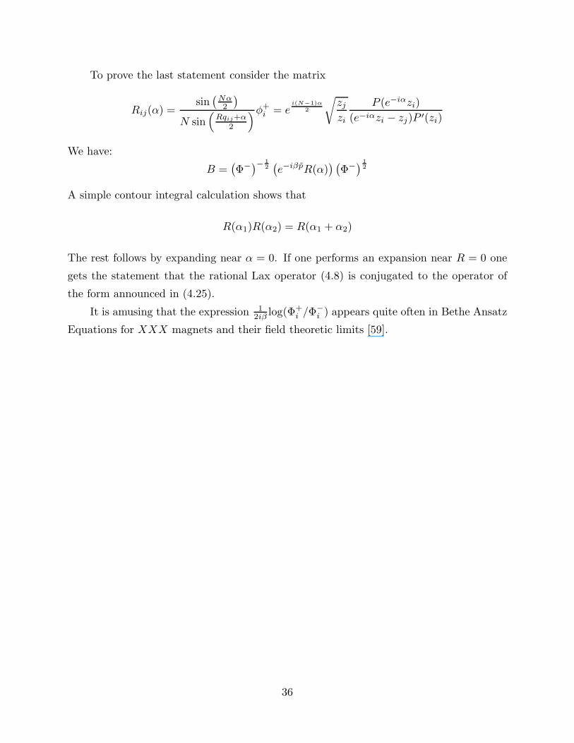
To prove the last statement consider the matrix

Rij(α) =sin

(Nα2

)

N sin(

Rqij+α2

)φ+i = e

i(N−1)α

2

√zj

zi

P (e−iαzi)

(e−iαzi − zj)P ′(zi)

We have:

B =(Φ−)− 1

2(e−iβpR(α)

) (Φ−) 1

2

A simple contour integral calculation shows that

R(α1)R(α2) = R(α1 + α2)

The rest follows by expanding near α = 0. If one performs an expansion near R = 0 one

gets the statement that the rational Lax operator (4.8) is conjugated to the operator of

the form announced in (4.25).

It is amusing that the expression 12iβ log(Φ+

i /Φ−i ) appears quite often in Bethe Ansatz

Equations for XXX magnets and their field theoretic limits [59].

36

5. Gauge theories and duality in integrable systems

5.1. Old approach: many-body systems as low-dimensional gauge theories

It is a fruitful approach to think of the many-body system as of the gauge theory of

a certain kind. Namely, the particles of the model can be identified (sometimes) with the

eigenvalues of the Wilson loops in the theory and the gauge dynamics becomes a dynamics

of the particles. Of course, in the real four dimensional world the gauge field has infinitely

many degrees of freedom and we don’t expect to see any tractable quantum mechanical

system unless we have a principle which allows us to restrict the dynamical problem to

a finite number of degrees of freedom. The simplest case is the case of low-dimensional

gauge theory, where the gauge field simply doesn’t have propagating degrees of freedom.

Consider, for example, two dimensional Yang-Mills theory with a gauge group G = U(N).

When formulated on a circle of radius R in the Hamiltonian formalism the theory has as

a phase space the space of gauge fields A(x) on the circle and their duals - chromoelectric

fields E(x). The gauge group acts on (E,A) as follows:

(E,A) → (g−1Eg, g−1∂xg + g−1Ag) (5.1)

leading to the Gauss law ∂xE + [A,E], which is nothing but the moment map from the

section 4.2. We can go to the gauge where A is a constant (w.r.t. x) diagonal matrix

A = diag(q1, . . . , qN ) (5.2)

Here are our particles. The time evolution makes qi to move and depending on the cir-

cumstances such as the presence of the sources like J (which correspond to the time-like

Wilson lines) one gets the Hamiltionian system of the kind we described and studied.

The large gauge transformations shift qi’s by integer multiples of 1R

making them live

on a circle of radius 12πR

. One can get more complicated examples by deforming the

model as follows. Replace S1 by T2, E by the second component of the gauge field

along the torus, the symplectic form being∫T2 TrδA ∧ δA. Then the Gauss law becomes

FA = ∂xAy − ∂yAx + [Ax, Ay]. Setting it to zero allows to diagonalize Ax, Ay simultane-

ously: (Ax

Ay

)= diag

((p1

q1

), . . . ,

(pN

qN

))(5.3)

Here, xi and yi do not Poisson-commute, although both live on circle. One gets, therefore

a system of relativistic partcles on a circle. The radius of the circle is 12πRx

, the speed of

37

light is Ry. The gauge theory this model corresponds to is known as Chern-Simons theory

on a torus (perhaps with punctures).

One can go higher in dimensions with some care. For example, by considering super-

symmetric N = 2 theory in d = 4 with compact space M3 one gets a quantum mechanics

on the moduli space of monopoles in IR3.

5.2. New approach: many-body systems in supersymmetric gauge theories

Recent progress in the understanding of non-perturbative phenomena emerged after

the work of Seiberg and Witten on four dimensional N = 2 SYM [12] and works of Seiberg

and his collaborators on N = 1 d = 4 theories. The major tool in these studies is the

low energy effective Lagrangian which is constrained by two priniciples - the holomorphy

of chiral objects and electric-magnetic duality. It is the electric-magnetic duality which

makes the integrable systems to appear in the solutions to the gauge theories.

In particular, one can argue on the general grounds [18] that any N = 2 supersym-

metric gauge theory in four dimensions corresponds to a certain integrable system in the

holomorphic sense. The point is that the Coulomb branch of the theory parameterizes

the family of abelian varieties (whose period matrix coincides with the matrix of coupling

constants of the effective low-energy abelian theory). Moreover the total space must carry

a holomorphic symplectic form ω, whose integral along the cycle in the fiber gives rise to

a derivative of the central charge of a BPS representation of N = 2 susy algebra along

the base. Moreover the abelian varieties must be Lagrangian with respect to ω.

The integrable systems corresponding to a large number of field theories are identified.

In particular, the low-energy theory of the pure N = 2 SU(Nc) SYM is governed by

the ANc−1 periodic (or affine) Toda system. The N = 2 theory with a massive adjoint

hypermultiplet corresponds to the elliptic Calogero-Moser system, where the mass (which

is naturally a complex parameter in the N = 2 theory) is identified with the coupling

constant. The theory is UV finite (in fact, it is softly broken N = 4 theory) and therefore

has as another modulus – the ultra-violet coupling τ which enters the integrable model as

the modulus of the curve. Another theories which were mentioned so far are the relativistic

generalizations of those two. These correspond to five dimensional gauge theories with the

same number of supercharges, compactified on a circle of a finite radius R. The speed of

light of the relativistic model is proportional to the inverse radius 1R

of the circle. For the

theories with fundamental matter the firm identification with the integrable systems has

been made in four [28][60] as well as in five and six dimensions [60].

38

In some cases the dualities suggested by the integrable systems are not obvious on

the field theory side. We plan to return to more detailed treatment of these cases (which

involve six dimensional theories) in the future.

5.3. Dualities in field theories vs. dualities in many-body systems

Dualities in the old approach. Let us start with the two-dimensional Yang-Mills the-

ory with the gauge coupling g2 formulated on a Riemann surface of area A. It was shown

by E. Witten in [61] that the perturbative in g2A part of the correlation functions in this

(non-supersymmetric) theory coincides with the correlation functions of certain observables

in twisted N = 2 supersymmetric two-dimensional Yang-Mills theory.

Among the twisted supercharges of the latter theory one finds a scalar Q which annihi-

lates the complex scalar φ in the vector multiplet. The observables constructed out of the

gauge invariant functions of φ and their descendants can be mapped to certain observables

in non-supersymmetric theory.

As we discussed above, when Yang-Mills theory is formulated on a cylinder with the

insertion of an appropriate time-like Wilson line, it is equivalent to the Sutherland model

describing a collection of N particles on a circle. The observables Trφk of the previous

paragraph are precisely the integrals of motion of this system.

One can look at other supercharges as well. In particular, when the theory is for-

mulated on a cylinder there is another class of observables annihilated by a supercharge.

One can arrange the combination of supercharges which will annihilate the Wilson loop

operator. By repeating the procedure similar to the one in [61] one arrives at the quantum

mechanical theory whose Hamiltonians are generated by the spatial Wilson loops. This

model is nothing but the rational Ruijsenaars-Schneider many-body system.

The duality between these two systems is a consequence of the fact that when lifted

to the supersymmetric model both field theories become equivalent to the same N = 2

super-Yang-Mills theory in two dimensions.

The self-duality of trigonometric Ruijsenaars system has even more transparent physi-

cal meaning. Namely, the field theory whose quantum mechanical avatar is the Ruijsenaars

system is three dimensional Chern-Simons theory on T2 ×R1 with the insertion of an ap-

propriate temporal Wilson line and spatial Wilson loop. It is the freedom to place the

latter which leads to several equivalent theories. The group of (self-)dualities of this model

is very big and is generated by the transformations S and T (4.31).

39

In short, the duality reveals here itself as a consequence of Lorentz invariance of the

underlying field theory.

Duality in the new approach. The new approach deals with supersymmetric gauge

theories in three, four, five and six dimensions. Perhaps the richest case is the six dimen-

sional theory compactified on a three dimensional torus T3 down to three dimensions.

As was discussed extensively in [15] in case where two out of three radii of T3 are much

smaller then the third one R the effective three dimensional theory is a sigma model with

the target space X being the hyper-kahler manifold (in particular, holomorphic symplectic)

which is a total space of algebraic integrable system. The complex structure in which X is

the algebraic integrable system is independent of the radius R while the Kahler structure

depends on R in such a way that the Kahler class of the abelian fiber is proportional to

1/R.

The duality of the integrable systems shows up in the gauge theories in the several

ways.

First of all AA duality the well-known phenomenon in the four dimensional N = 2

gauge theory which was observed and exploited in [12] and then later on in the plenty of

works. The low-energy effective theory has different sets of relevant degrees of freedom

over different regions of the moduli space of vacua. The transformations between differ-

ent descriptions go through the electric-magnetic duality on the gauge field side which is

accompanied by supersymmetry by a AA-type duality on the scalar side. Although this

duality is connected with the electric-magnetic symmetry which is not realized geometri-

cally in four dimensions, it does become geometric when the theory is lifted to a tensor

theory in six dimensions [62].

The duality of the AC type is also present and is rather interesting. As one varies the

moduli of T3 the geometry of X varies as well. In particular, different four dimensional

theories can flow to the same three dimensional theory. This is where the AC duality in

the integrable systems shows up.

For example, a certain scaling limit of the five dimensional SU(N) theory with massive

adjoint hypermultiplet, compactified on a circle seems to be equivalent/dual to four di-

mensional SU(N) theory with massive adjoint hypermultiplet when instanton corrections

are turned off in both theories.

The theory in three dimensions which came from four dimensions upon a compact-

ification on a circle whose low-energy effective action describes only abelian degrees of

40

freedom can be always dualized to the theory of scalars/spinors only, due to the vector-

scalar duality in three dimensions. In this way different sets of vector and hypermultiplets

in four dimensions can lead to the same three dimensional theory (one of the examples of

such symmetries is provided by the three dimensional mirror symmetry [63][64]).

One can also use the AC duality to establish the following fact. Consider two AC dual

integrable systems. Consider three dimensional N = 4 supersymmetric gauge theory whose

Higgs branch is X - the phase space of these systems. Then two N = 2 supersymmetric

theories whose spaces of scalars are both X but the superpotentials are taken from the

sets of Hamiltonians of the first and the second systems respectively are dual to each other

in the sense that both flow in the UV/IR (depending on the whether these Hamiltonians

correspond to the relevant or irrelevant operators) to the same theory.

We are certain that there are more applications of the notion of duality in integrable

systems both in the theory of integrability itself and in the physics, gauge theories being

the arena for the most immediate ones.

41

References

[1] N. Hitchin, “Stable Bundles And Integrable Systems”, Duke Math. Journal, Vol. 54,

No. 1 (1987)

[2] V. Knizhnik, A. Zamolodchikov, Nucl. Phys. B 247 (1984) 83-103;

D. Bernard, Nucl. Phys. B303 (1988) 77, B309 (1988), 14

[3] A. Losev, “Coset construction and Bernard Equations”, CERN-TH.6215/91

[4] D. Ivanov, “ Knizhnik-Zamolodchikov-Bernard equations on Riemann surfaces”, hep-

th/9410091;

“Knizhnik-Zamolodchikov-Bernard equations as quantization of a nonstationary

Hitchin system”, hep-th/9610207

[5] L. Schlesinger, “ Uber eien Klasse von Differentialsystemen beliebiger Ordnung mit

festen kritischen Punkten”, Journal fur die reine und angewandte Mathematik, Bd.

CXLI (1912), pp. 96-145

[6] R. Garnier, “Sur une classe de systemes differentiels Abeliens deduits de la theorie

des equations lineares”, Rend. del Circ. Matematice Di Palermo, 43, vol. 4 (1919)

[7] M. Gaudin, Jour. Physique, 37 (1976), 1087-1098

[8] B. Feigin , E. Frenkel, N. Reshetikhin, “Gaudin Model, Critical Level and Bethe

Ansatz”, CMP 166 (1995), 27-62

[9] H. Ooguri and C. Vafa, “Self-Duality and N = 2 String Magic,” Mod.Phys.Lett. A5

(1990) 1389-1398;

“Geometry of N = 2 Strings,” Nucl.Phys. B361 (1991) 469-518.

[10] V. Novikov, M.A. Shifman, A.I. Vainshtein, V.I. Zakharov, “Exact Gell-Mann-

Low Function of Supersymmetric Yang-Mills Theories From Instanton Calculus”,

Nucl.Phys.B 229 (1983) 381;

“Beta Function in Supersymmetric Gauge Theories: Instantons Versus Traditional

Approach”, Phys.Lett.B 166 (1986) 329

[11] N. Seiberg, “Supersymmetry and Non-perturbative Beta-Functions”, Phys. Lett.B206

(1988) 75

[12] N. Seiberg, E. Witten, “Electric-Magnetic Duality, Monopole Condensation, And Con-

finement in N = 2 Supersymmetric Yang-Mills Theory ” Nucl. Phys. B426 (1994)

19-52 (and erratum - ibid. B430 (1994) 485-486 );

“Monopoles, Duality and Chiral Symmetry Breaking in N = 2 Supersymmetric

QCD”, hep-th/9408099, Nucl. Phys. B431 (1994) 484-550.

[13] K. Intriligator and N. Seiberg, “Phases of N = 1 supersymmetric gauge theories in

four dimensions”, hep-th/9408155;

K. Intriligator, N. Seiberg, and S. H. Shenker, “Proposal for a Simple Model of

Dynamical SUSY Breaking”, hep-ph/9410203;

42

N. Seiberg, “Electric-Magnetic Duality in Supersymmetric Non-Abelian Gauge The-

ories”, hep-th/9411149;

K. Intriligator and N. Seiberg “Duality, Monopoles, Dyons, Confinement and Oblique

Confinement in Supersymmetric SO(Nc) Gauge Theories”, hep-th/9503179

[14] P.C. Argyres, A.E. Farragi, “The Vacuum Structure and Spectrum of N = 2 Super-

symmetric SU(N) Gauge Theory”, hep-th/9411057;

A. Klemm, W. Lerche, S. Theisen and S. Yankielowicz, “Simple Singularities and

N = 2 Supersymmetric Yang-Mills Theory”, hep-th/9411048

[15] N. Seiberg, E. Witten, “Gauge Dynamics and Compactification to Three Dimensions”,

hep-th/9607163

[16] A. Gorsky, I. Krichever, A. Marshakov, A. Morozov, A. Mironov, “Integrablity

and Seiberg-Witten Exact Solution”, hep-th/9505035, Phys. Lett. B355 (1995) 466-

474

[17] E. Martinec and N. Warner, “Integrable systems and supersymmetric gauge theory”,

hep-th/9509161, Nucl. Phys. B459, 97

[18] R. Donagi, E. Witten, “Supersymmetric Yang-Mills Theory and Integrable Systems”,

hep-th/9510101, Nucl.Phys.B460 (1996) 299-334

[19] M. Olshanetsky, A. Perelomov, Inv. Math. 31 (1976), 93

[20] M. Olshanetsky, A. Perelomov, Phys. Rep. 71 (1981), 313

[21] E. Witten, “String theory dynamics in various dimensions”, hep-th/9503124, Nucl.Phys.

B 443 (1995), 85

[22] J. Schwarz, “The Power of M -Theory”, Phys. Lett. B377 (1996) hep-th/9508143

[23] A. Gorsky, N. Nekrasov, V. Rubtsov, “Separation of variables, Hilbert Schemes and

D-Branes”, hep-th/9901089

[24] M. Douglas, “Superstring Dualities, Dirichlet Branes and the Small Scale Structure

of Space-Time”, hep-th/9610041

[25] M. Douglas, “Gauge Fields and D-branes”, hept-h/9604198

[26] O. Babelon, E. Billey, I. Krichever, M. Talon, “Spin generalization of the Calogero-

Moser system and the Matrix KP equation”, hep-th/9411160

[27] I. Krichever, A. Zabrodin, “Spin Generalization of Ruijsenaars-Schneider model,

Non-abelian Toda Chain and Representations of Sklyanin Algebra”, hep-th/9505039

[28] A. Gorsky, A. Marshakov, A. Mironov, A. Morozov, “N = 2 Supersymmetric QCD

and Integrable Spin chains: Rational Case Nf < 2Nc ”, hep-th/9603140, Phys.Lett.

B 380 (1996) 75

[29] J. Polchinski, “Dirichlet-branes and Ramond-Ramond charges”, hep-th/9510017,

Phys.Rev.Lett. 75, 4724

[30] J. Polchinski, “TASI lectures on D-branes”, hep-th/9611050

[31] C. Vafa, “Lectures on strings and dualities”, hep-th/9702201

43

[32] P. Etingof, “Quantum integrable systems and representations of Lie algebras”, hep-

th/9311132

[33] P. Etingof, A. Kirillov, Jr., “Macdonald polynomials and representations of quantum

group’, hep-th/9312103;

“Representation-theoretic proof of the inner product and symmetry identities for Mac-

donald’s polynomials”, hep-th/9410169

[34] P. Etingof, A. Kirillov, Jr., “On the affine analogue of Jack’s and Macdonald’s poly-

nomials”, hep-th/9403168

[35] A. Beilinson, V. Drinfeld, “Quantization of Hitchin’s fibration and Langlands’ pro-

gram”, in ‘Algebraic and geometric methods in mathematical physics’ (Kaciveli, 1993),

3–7, Math. Phys. Stud., 19, Kluwer Acad. Publ., Dordrecht, 1996.

[36] G. Arutyunov , S. Frolov and P. Medvedev “Elliptic Ruijsenaars-Schneider model

from the cotangent bundle over the two-dimensional current group”, hep-th/9608013

, J. Math. Phys. 38 (1997) 5682 ;

“Elliptic Ruijsenaars-Schneider model via the Poisson reduction of the affine Heisen-

berg double”, hep-th/9607213 , J. Phys. A (1997) 505

[37] V. Arnol’d, “Mathematical methods in Classical Mechanics”, Springer-Verlag, NY

1989

[38] R. Donagi, “Seiberg-Witten Integrable Systems”, alg-geom/9705010

[39] N. Nekrasov, “Five dimensional gauge theories and relativistic integrable systems”,

hep-th/9609219, Nucl. Phys. B 531 (1998) 323-344

[40] O. Ganor, D. Morrison, N. Seiberg, “Branes, Calabi-Yau Spaces and Compactification

of Six Dimensional E8 Theory”, hep-th/9610251

[41] S. Novikov, A. Veselov, Proc. Steklov Math. Institute, 3 (1985) 53-65

[42] L. Landau, E. Lifshitz, “Quantum Mechanics (Non-relativistic theory)”, Pergamon

Press, 1977

[43] P. Etingof, I. Frenkel, “Central Extensions of Current Groups in Two Dimensions”,

CMP 165 (1994) 429-444

[44] G. Bonelli, M. Matone, “Nonperturbative Relations in N=2 SUSY Yang-Mills and

WDVV equation”, Phys. Rev. Lett.77 (1996) 4712, hep-th/9605090

[45] F. Calogero, J.Math.Phys. 12 (1971) 419

[46] J. Moser, Adv.Math. 16 (1975), 197-220;

[47] B. Sutherland, Phys. Rev. A5 (1972), 1372-1376;

[48] S.N.M. Ruijsenaars, H. Schneider, “A New Class of Integrable Systems and Its Rela-

tion to Solitons”, Ann. of Physics 170 (1986), 370-405

[49] S. Ruijsenaars, “Complete Integrability of Relativistic Calogero-Moser Systems and

Elliptic Function Identities”, CMP 110 (1987), 191-213

[50] S. Ruijsenaars, “Action-Angle Maps and Scattering Theory for Some Finite-

Dimensional Integrable Systems”, CMP 115 (1988), 127-165

44

[51] S. Ruijsenaars, “Finite-Dimensional Soliton Systems”, in ‘Integrable and Super-

Integrable Systems’, eds. B. Kupershmidt, World Scientific, Singapore, 1986

[52] S. Ruijsenaars, “Action-Angle Maps and Scattering Theory for Some Finite-

Dimensional Integrable Systems II, III”, Publ. RIMS, Kyoto Univ 30 (1994), 865-

1008 and 31 (1995), 247-353

[53] D. Kazhdan, B. Kostant and S. Sternberg, Comm. on Pure and Appl. Math., vol.

XXXI, (1978), 481-507

[54] A. Perelomov, “Integrable Systems of Classical Mechanics and Lie Algebras”, Moscow,

‘Nauka’, 1990 [in Russian]

[55] A. Gorsky, N. Nekrasov, “Hamiltonian systems of Calogero type and Two Dimen-

sional Yang-Mills Theory”, Nucl. Phys. B 414 (1994), 213-238, hep-th/9304047

[56] A. Gorsky, N. Nekrasov, “Relativistic Calogero-Moser model as gauged WZW the-

ory”, hep-th/9401017, Nucl.Phys. B 436 (1995) 582-608

[57] V. Fock, A. Rosly, “Flat connections and polyubles”, Teor. Math. Fiz. 95 (1993) 2,

228-238.

[58] I. Cherednik, “Difference-elliptic operators and root systems”, hep-th/9410188

[59] L. Faddeev, “How Bethe Ansatz Works for Integrable Model”, 1995 Les-Houches

lecture notes, hep-th/9605187

[60] A. Gorsky, S.Gukov and A.Mironov, “Multiscale N = 2 susy field theories, integrable

systems and their stringy/brane origin”, hep-th/9707120, Nucl. Phys. B 517 (1998)

409 ;

“Integrable spin chains and supersymmetric Yang-Mills theories in higher dimensions”,

hep-th/9710239, Nucl.Phys. B 518 (1998) 683

[61] E. Witten, “On Quantum gauge theories in two dimensions,” CMP 141 (1991) 153;

“Two dimensional gauge theories revisited”, J. Geom. Phys. 9 (1992) 303-368

[62] E. Witten, “Some Comments on String Dynamics”, hep-th/9507121

[63] K. Intrilligator, N. Seiberg, “Mirror symmetry in three dimensional gauge theories”,

hep-th/9607207, Phys. Lett. B387 (1996) 513

[64] A. Kapustin, “Solution of N = 2 gauge theories via compactification to three dimen-

sions”, hep-th/9804069, Nucl. Phys. B534 (1998) 531

45