Entanglement and defect entropies ingauge/gravity duality

Mario Flory

Munchen 2016

Entanglement and defect entropies ingauge/gravity duality

Mario Flory

Dissertation

an der Fakultat fur Physik

der Ludwig–Maximilians–Universitat

Munchen

vorgelegt von

Mario Flory

aus Neustadt an der Aisch

Munchen, den 5. April 2016

Erstgutachter: Prof. Dr. Johanna Erdmenger

Zweitgutachter: Prof. Dr. Dieter Lust

Tag der mundlichen Prufung: 13.07.2016

Contents

Zusammenfassung xi

Abstract xiii

1 Introduction 1

2 Holography 132.1 Holography and the laws of gravity . . . . . . . . . . . . . . . . . . . . . . 13

2.1.1 Black hole thermodynamics and entropy bounds . . . . . . . . . . . 132.1.2 The holographic principle . . . . . . . . . . . . . . . . . . . . . . . 162.1.3 Covariant entropy bound . . . . . . . . . . . . . . . . . . . . . . . . 172.1.4 Anti-de Sitter spacetime . . . . . . . . . . . . . . . . . . . . . . . . 19

2.2 The AdS3/CFT2 duality . . . . . . . . . . . . . . . . . . . . . . . . . . . . 212.3 Maldacena’s AdS5/CFT4 duality . . . . . . . . . . . . . . . . . . . . . . . 24

2.3.1 Open string construction . . . . . . . . . . . . . . . . . . . . . . . . 242.3.2 Closed string construction . . . . . . . . . . . . . . . . . . . . . . . 262.3.3 The duality . . . . . . . . . . . . . . . . . . . . . . . . . . . . . . . 29

2.4 Epilogue: comparison to optical holography . . . . . . . . . . . . . . . . . 34

3 Entanglement entropy and holography 393.1 Definition . . . . . . . . . . . . . . . . . . . . . . . . . . . . . . . . . . . . 393.2 Holographic entanglement entropy . . . . . . . . . . . . . . . . . . . . . . . 413.3 Black hole entropy and thermofield double states . . . . . . . . . . . . . . 443.4 The replica method . . . . . . . . . . . . . . . . . . . . . . . . . . . . . . . 49

4 Entanglement entropy in higher curvature theories 534.1 Introduction . . . . . . . . . . . . . . . . . . . . . . . . . . . . . . . . . . . 534.2 New massive gravity . . . . . . . . . . . . . . . . . . . . . . . . . . . . . . 554.3 Gauss-Bonnet gravity . . . . . . . . . . . . . . . . . . . . . . . . . . . . . . 594.4 The causal influence argument . . . . . . . . . . . . . . . . . . . . . . . . . 63

vi Contents

5 Backreaction in holographic models of boundary CFTs 695.1 Holographic models of boundary CFTs . . . . . . . . . . . . . . . . . . . . 695.2 Energy conditions and their impact on the bulk geometry . . . . . . . . . . 71

5.2.1 Decomposition of the energy-momentum tensor . . . . . . . . . . . 715.2.2 Energy conditions . . . . . . . . . . . . . . . . . . . . . . . . . . . . 725.2.3 A corollary to the barrier theorem . . . . . . . . . . . . . . . . . . . 735.2.4 AdS and BTZ backgrounds . . . . . . . . . . . . . . . . . . . . . . 76

5.3 Exact solutions . . . . . . . . . . . . . . . . . . . . . . . . . . . . . . . . . 805.3.1 Constant tension solutions . . . . . . . . . . . . . . . . . . . . . . . 805.3.2 Perfect fluid models . . . . . . . . . . . . . . . . . . . . . . . . . . . 83

6 Entanglement entropy in a holographic Kondo model 896.1 Field theory and top-down model . . . . . . . . . . . . . . . . . . . . . . . 89

6.1.1 Field theory . . . . . . . . . . . . . . . . . . . . . . . . . . . . . . . 896.1.2 Top-down model . . . . . . . . . . . . . . . . . . . . . . . . . . . . 92

6.2 The bottom-up Kondo model . . . . . . . . . . . . . . . . . . . . . . . . . 946.3 Backreaction in the Kondo model . . . . . . . . . . . . . . . . . . . . . . . 97

6.3.1 The Israel junction conditions . . . . . . . . . . . . . . . . . . . . . 986.3.2 Equations of motion . . . . . . . . . . . . . . . . . . . . . . . . . . 101

6.4 Entanglement and defect entropy . . . . . . . . . . . . . . . . . . . . . . . 1036.4.1 Energy conditions in the Kondo model . . . . . . . . . . . . . . . . 1036.4.2 Entanglement entropy in the Kondo model . . . . . . . . . . . . . . 1056.4.3 The holographic g-theorem . . . . . . . . . . . . . . . . . . . . . . . 109

6.5 An analytical approximation formula for entanglement entropy . . . . . . . 1106.6 An outlook on complexity . . . . . . . . . . . . . . . . . . . . . . . . . . . 1166.7 T = 0 behaviour . . . . . . . . . . . . . . . . . . . . . . . . . . . . . . . . . 118

7 Outlook 123

A Extrinsic curvature quantities 127A.1 Codimension two hypersurfaces . . . . . . . . . . . . . . . . . . . . . . . . 127A.2 Codimension one hypersurfaces . . . . . . . . . . . . . . . . . . . . . . . . 128

B Corollary to the barrier theorem in higher dimensions 131

C Junction conditions for abelian Chern-Simons fields 135

Bibliography 141

Acknowledgements 163

List of Figures

1.1 A holographic Kondo model . . . . . . . . . . . . . . . . . . . . . . . . . . 7

2.1 Geometrical setup for the Bousso bound . . . . . . . . . . . . . . . . . . . 182.2 A stack of D3-branes . . . . . . . . . . . . . . . . . . . . . . . . . . . . . . 252.3 Black brane in 10 dimensions . . . . . . . . . . . . . . . . . . . . . . . . . 28

3.1 Ryu-Takayanagi prescription . . . . . . . . . . . . . . . . . . . . . . . . . . 423.2 Example of a holographic entanglement entropy calculation . . . . . . . . . 443.3 Entangling curves in a black hole background . . . . . . . . . . . . . . . . 453.4 Conformal diagram of a static AdS black hole . . . . . . . . . . . . . . . . 463.5 Closed extremal curves in black hole backgrounds . . . . . . . . . . . . . . 483.6 Illustration of the replica method . . . . . . . . . . . . . . . . . . . . . . . 50

4.1 Types of additional closed extremal surfaces in new massive gravity . . . . 594.2 Parameter space of new massive gravity . . . . . . . . . . . . . . . . . . . . 604.3 Illustration of causal shadows . . . . . . . . . . . . . . . . . . . . . . . . . 644.4 Domain of dependence of a boundary region A . . . . . . . . . . . . . . . . 654.5 Application of the causal influence argument to a black hole spacetime . . 66

5.1 An AdS/BCFT model . . . . . . . . . . . . . . . . . . . . . . . . . . . . . 705.2 Illustration of the barrier theorem . . . . . . . . . . . . . . . . . . . . . . . 755.3 Geodesic normal flow construction . . . . . . . . . . . . . . . . . . . . . . . 825.4 Brane embeddings for a perfect fluid model in a Poincare background . . . 855.5 Brane embeddings for a perfect fluid plus constant tension model in a BTZ

background . . . . . . . . . . . . . . . . . . . . . . . . . . . . . . . . . . . 86

6.1 Illustration of the Anderson impurity model . . . . . . . . . . . . . . . . . 906.2 Geometric setup of Israel junction conditions . . . . . . . . . . . . . . . . . 996.3 Israel junction conditions in standard coordinates and Gaussian normal co-

ordinates. . . . . . . . . . . . . . . . . . . . . . . . . . . . . . . . . . . . . 1006.4 Brane embeddings for the holographic Kondo model . . . . . . . . . . . . . 1056.5 Impurity entropy in the holographic Kondo model . . . . . . . . . . . . . . 1076.6 Exponential falloff of the impurity entropy . . . . . . . . . . . . . . . . . . 1096.7 Boundary entropy as a function of temperature. . . . . . . . . . . . . . . . 110

viii List of Figures

6.8 Geometrical approximation to the near horizon behaviour of the brane . . 1116.9 Numerical results for D(T ) . . . . . . . . . . . . . . . . . . . . . . . . . . . 1156.10 Proposal for relative complexity in the holographic Kondo model . . . . . . 1186.11 More realistic potentials for the Kondo model . . . . . . . . . . . . . . . . 121

B.1 Impact of the energy conditions on higher-dimensional AdS/BCFT models 132

C.1 Illustration of the derivation of junction conditions for the Abelian Chern-Simons field. . . . . . . . . . . . . . . . . . . . . . . . . . . . . . . . . . . . 136

C.2 Toy model illustrating the junction conditions for the Chern-Simons field . 139

List of Tables

2.1 Embedding of a D3-brane . . . . . . . . . . . . . . . . . . . . . . . . . . . 242.2 Symmetries in AdS5×S5/CFT4 . . . . . . . . . . . . . . . . . . . . . . . . 31

5.1 Energy conditions and embeddings in a BTZ background . . . . . . . . . . 78

6.1 D3-D5-D7-system of the holographic Kondo model . . . . . . . . . . . . . 92

Zusammenfassung

In dieser Dissertation untersuchen und verwenden wir geometrische Methoden zur Berech-nung von Verschrankungs-Entropie in Feldtheorien, die gemaß der Eichtheorie/Gravitations-Dualitat uber ein Gravitations-Dual verfugen. Die Hauptresultate dieser Arbeit ergebensich aus der Anwendung unserer Ergebnisse auf die Untersuchung von Verschrankungs-und Defekt-Entropien in einem holographischen Modell des Kondo-Effektes.

Die Eichtheorie/Gravitations-Dualitat ist eine wichtige Methode zur Untersuchung starkgekoppelter Systeme. Zunachst geben wir einen kurzen Uberblick uber die verwandtenIdeen des holographischen Prinzips und die Realisierung der AdS/CFT-Korrespondenz inStringtheorie (AdS steht hier fur Anti-de Sitter, und CFT steht fur Konforme Feldthe-orie, englisch conformal field theory). Außerdem besprechen wir das Konzept der Ver-schrankungs-Entropie und erklaren, wie diese Große holographisch berechnet werden kann.

Anschließend wenden wir moderne Methoden zur Berechnung von Verschrankungs-Entropiein Gravitationstheorien mit Termen hoherer Krummungsordnung auf spezielle Raumzeiten,im Besonderen auf stationare Schwarze Locher, an. Dabei stoßen wir auf analytischeLosungen fur die extremalen Hyperflachen, die die Verschrankungs-Entropie bestimmen,welche sich um das Schwarze Loch winden. Wir argumentieren, dass diese Hyperflachenunphysikalisch sind, indem wir aufzeigen, dass sie bestimmte Kausalitatsbedingungen ver-letzen.

Weiterhin untersuchen wir die geometrischen Eigenschaften bestimmter Modelle fur Du-alitaten zwischen AdS-Raumen und Grenzflachen-CFTs, mit einem besonderen Augen-merk auf ein kurzlich vorgeschlagenes holographisches Modell des Kondo-Effektes. Einesder Hauptresultate dieser Dissertation wird darin bestehen, ein Verstandnis dafur zu er-langen, wie sich Energie-Bedingungen auf die moglichen Geometrien der hoherdimensio-nalen Raumzeit auswirken. Wir wenden dann die Ergebnisse dieser Untersuchungen imSpeziellen auf das Kondo-Modell an und insbesondere berechnen wir Verschrankungs- undDefekt-Entropien numerisch. Diese Großen konnen im Kontext des RG-Flusses, welchendas Kondo-Modell erfahrt, interpretiert werden. Es wird im Detail erlautert, inwiefern dasholographische Kondo-Modell Erwartungen aus Feldtheorie-Rechnungen erfullt und wiees verbessert werden konnte. Weiterhin gehen wir auf aktuelle Vorschlage zur Definitioneines holographischen Maßes fur Komplexitat ein. Dabei handelt es sich um einen Begriffaus der Quanteninformationstheorie. Die Arbeit endet mit einem Ausblick auf mogliche

xii Zusammenfassung

zukunftige Forschungsrichtungen.

Diese Dissertation basiert auf der Arbeit die der Autor als Doktorand unter der Betreuungdurch Prof. Dr. Johanna Erdmenger am Max-Planck-Institut fur Physik in Munchen imZeitraum vom 2. April 2013 bis zum 31. Marz 2016 durchgefuhrt hat. Die einschlagigenPublikationen lauten wie folgt:

[1] J. Erdmenger, M. Flory and C. Sleight, Conditions on holographic entangling surfacesin higher curvature gravity, JHEP 1406 (2014) 104, arXiv:1401.5075 [hep-th].

[2] J. Erdmenger, M. Flory and M. N. Newrzella, Bending branes for DCFT in twodimensions, JHEP 1501 (2015) 058, arXiv:1410.7811 [hep-th].

[3] J. Erdmenger, M. Flory, C. Hoyos, M. N. Newrzella and J. M. S. Wu, Entangle-ment Entropy in a Holographic Kondo Model, Fortsch. Phys. 64 (2016) 109–130,arXiv:1511.03666 [hep-th].

[4] J. Erdmenger, M. Flory, C. Hoyos, M. N. Newrzella, A. O’Bannon and J. Wu, Holo-graphic impurities and Kondo effect, arXiv:1511.09362 [hep-th]

Abstract

In this thesis we investigate and use geometrical prescriptions for the calculation of en-tanglement entropy in field theories that have a gravity dual according to gauge/gravityduality. The main results of this work will arise from the application of our findings to thestudy of entanglement and defect entropies in a holographic model of the Kondo effect.

Gauge/gravity duality is an important tool for the study of strongly coupled systems.We give a short review over the related idea of the holographic principle and the realisa-tion of the AdS/CFT correspondence in string theory. We also introduce the concept ofentanglement entropy and review the methods of holographically calculating it.

We then apply recent prescriptions for calculating holographic entanglement entropy ingravitational theories with higher curvature terms to specific example spacetimes, suchas stationary black holes, and obtain analytical solutions for extremal surfaces definingentanglement entropy that wrap around the black holes. We argue that these surfaces areunphysical by discussing how they violate certain well motivated causality constraints.

We then investigate the geometrical properties of certain models of dualities between AdSspaces and boundary CFTs, with a special interest in a recently proposed holographicmodel of the Kondo effect. Understanding the impact of energy conditions on the allowedbulk geometries will be one of the main results of this thesis. We then apply the knowledgegained from these studies to the specific Kondo model, and numerically calculate entan-glement and impurity entropies. These quantities can be interpreted in terms of the RGflow that the Kondo model undergoes. It will also be discussed in detail to which extendthe holographic model reproduces field theory expectations, and how it can be improved.Furthermore, we investigate recent proposals of defining holographic measures of complex-ity. This is a quantity in quantum information theory. We end with an outlook on possiblefuture research directions.

This thesis is based on the research that the author carried out as a PhD student underthe supervision of Prof. Dr. Johanna Erdmenger at the Max Planck Institute for Physicsin Munich, Germany, between the 2nd of April 2013 and the 31st of March 2016. Therelevant publications are:

[1] J. Erdmenger, M. Flory and C. Sleight, Conditions on holographic entangling surfacesin higher curvature gravity, JHEP 1406 (2014) 104, arXiv:1401.5075 [hep-th].

xiv Abstract

[2] J. Erdmenger, M. Flory and M. N. Newrzella, Bending branes for DCFT in twodimensions, JHEP 1501 (2015) 058, arXiv:1410.7811 [hep-th].

[3] J. Erdmenger, M. Flory, C. Hoyos, M. N. Newrzella and J. M. S. Wu, Entangle-ment Entropy in a Holographic Kondo Model, Fortsch. Phys. 64 (2016) 109–130,arXiv:1511.03666 [hep-th].

[4] J. Erdmenger, M. Flory, C. Hoyos, M. N. Newrzella, A. O’Bannon and J. Wu, Holo-graphic impurities and Kondo effect, arXiv:1511.09362 [hep-th]

Chapter 1

Introduction

From clockworks to geometry and information

The goal of natural sciences is to describe the world around us in exact scientific terms,often by uncovering fundamental laws of nature and phrasing them in an unambiguousmathematical language, thereby enabling scientists to make predictions about future eventsin nature or laboratory environments. Ultimately, the natural sciences, specifically physics,have to be applied to the universe as a whole. In this endeavour, it is not surprising that,instead of starting from scratch, people have often derived inspiration from the ideas ofscience and technology that were prevalent at the time. The deterministic laws of celestialmotion and Newtonian mechanics have, for example, often caused scientists to liken theuniverse to a clockwork. In contrast, during the last century, the analogy of the universeas a (quantum) computer seems to have grown popular.

A little more than 100 years ago, Albert Einstein’s general theory of relativity1, introducedthe idea into theoretical physics that events in the universe are not taking place on a fixedstage, but that spacetime itself is a dynamical quantity, and has to play an important partin the physics of the universe. This was already an enormous paradigm shift, but it didn’ttake long before scientists such as Oskar Klein and Theodor Kaluza proposed that the ideaof dynamical spactime geometry could lead the way to a unification of general relativityand electromagnetism. Although due to certain problems of this approach and the rise ofquantum field theory these early ideas have fallen somewhat out of favour shortly aftertheir advent,2 they have arguably seen a strong comeback with the necessity of handlingthe extra dimensions that string theory proposes.

In the 1950s, the idea of dynamical geometry as the fundamental property of nature madeits return to (classical) theoretical physics with Wheelers idea of geometrodynamics [7, 8],culminating in the slogan “physics is geometry” [8]. This program proposed that, for

1Just recently confirmed once more by the direct detection of a gravitational wave [5].2For an excellent overview over the early history of general relativity and Kaluza Klein theory, see [6].

2 1. Introduction

example, point charges could be seen as the ends of tiny wormholes from which the fieldlines of a source-free electromagnetic field emerge.

These ideas attracted some amount of interest at the time, only to fall out of favourthereafter, only to be revived once more in a slightly different way under the modern slogan“ER=EPR” (see [9–13] for a partial list of references). This idea notes certain fundamentalsimilarities between the physical properties of entangled particles (EPR pairs) and blackholes (defined by the geometry of Einstein-Rosen (ER) bridges) and proposes that thisis not a coincidence, but in fact a fundamental duality between these two phenomena.This would mean that entanglement, one of the core phenomena of quantum physics andquantum information theory, can be understood in terms of geometry and topology. Howcan such a bold claim be made with so much confidence? The reason is that this is notan isolated qualitative idea, but it is motivated and in some cases derived from a muchbroader, more fundamental and, most importantly, more quantitative framework, namelythe ideas of holography and gauge/gravity duality.

Holography

The ideas of holography arise from the need to formulate a consistent theory of thermo-dynamics in a world that allows for black holes to exist. Black holes are solutions to theequations of Einstein’s gravity (or similar theories) that have a non-trivial causal struc-ture, i.e. there are regions in the black hole spacetime that cannot send a signal out tothe region infinitely far away from the black hole. Such objects can only arise in a theorywhere the speed of communication has an upper bound (the speed of light in Einstein’stheory) and the spacetime metric (the mathematical object determining the trajectoriesof information carrying signals) is a dynamical quantity, not being fixed to be a simplebackground structure. Even more, such objects are not only theoretical constructs allowedby the mathematics of Einstein’s theory, but also have they likely been observed to existin nature [5]. The consistency of the physics of such objects with the well known laws ofthermodynamics is hence an interesting and important question, the study of which wasstarted in [14–16]. The result of this work was the realisation that not only is it necessaryto assign entropy to black holes, but that this entropy has to scale like the surface area ofthe black hole. This is in contrast to non-gravitational systems where the thermodynamicentropy, being an extensive quantity, scales like the volume. This groundbreaking resulthas led to deep investigations into the thermodynamics of black holes and quantum fieldtheory in curved spacetimes. Also, it has led to the idea that there should be upper boundson the amount of entropy (or information) that can be stored in physical systems, depend-ing on the characteristics of the system such as energy content or size [17–19]. Simplyspeaking, whenever someone tries to violate these bounds by storing too much entropyin a given system, nature automatically intervenes by forming a black hole. This led tothe proposal [18, 19] that a consistent theory unifying the laws of gravity and the lawsof quantum physics should obey the holographic principle, the principle that the number

3

of degrees of freedom of a given spacetime region scales like its surface area, not like itsvolume.

The best current candidate for a unified theory of quantum gravity is string theory (see[20–24] for introductory texts), and indeed it has been shown [25–27] that the holographicprinciple is realised in string theory in the form of an Anti-de Sitter/conformal field the-ory (AdS/CFT) correspondence. Specifically, the most well known example studied in [25]proposes a duality between type IIB superstring theory on an AdS5×S5 background andN = 4 SU(N) super Yang-Mills theory in 3 + 1 dimensions, which is a CFT. The formertheory is (in general) a theory of quantum gravity and hence its foundational principlesand properties must currently be considered to be mysterious, but the latter one, in con-trast, is a quantum field theory and hence in principle well understood. This is how theAdS/CFT correspondence encodes the holographic principle, a quantum gravity theory in(after compactification) (d + 1) + 1 dimensions is formulated as a d + 1-dimensional fieldtheory, such that the entropies in both theories will scale as lengthd.

Although we wrote above that in general the mathematical principles of quantum fieldtheory are much better understood than those of quantum gravity, we will see later thatthe best understood form of Maldacena’s AdS5/CFT4 correspondence requires us to workin a parameter range where the CFT is strongly coupled, making computations hard inpractice. On the other hand, the quantum gravity theory becomes weakly coupled classicalgravity in this case, and is hence tractable. The AdS5/CFT4 correspondence and similarmodels of AdS/CFT duality and generalisations thereof, going by the name gauge/gravitydualities, then provide a new way of studying strongly coupled systems. This topic isnotoriously hard due to the inapplicability of perturbation theory and the shortcomingsof lattice techniques. Successes of gauge/gravity duality techniques in this field involve,amongst many others, the following:

• Gauge/gravity duality naturally suggests an investigation of the information paradox,as the CFT that is dual to the quantum gravity theory in the bulk is manifestlyunitary [28].

• Using gauge/gravity techniques, it has been possible to derive the ratio of shearviscosity η to entropy density s,

η

s=

1

4π

~kB, (1.1)

for a wide class of holographic fluids [29,30]. Later, an entire field called fluid/gravitycorrespondence emerged in which the methods of holography, and in particular thephysics of black holes and event horizons, were applied to the study of fluids [31], seealso [32] for an overview.

• In fact, the result (1.1) has been conjectured to be a universal lower bound on η/sfor realistic systems [29, 30] (see also the review [33]), an idea fuelled by the factthat of all experimentally known fluids in nature it is the (strongly coupled) quark-gluon plasma (QGP) that comes closest to this bound, but it does not violate it

4 1. Introduction

[30, 33, 34]. Much work, often involving numerical simulations of dynamical bulkspacetimes, has been invested to apply gauge/gravity techniques to the study ofstrongly coupled plasmas and QGP phenomenology, which can experimentally bestudied in heavy ion collisions at accelerators such as LHC or RHIC. Apart fromthis problem of heavy ion collisions, gauge/gravity methods have also been appliedto other questions in quantum chromodynamics (QCD). For overviews of the variousattempts to create qualitative holographic duals of QCD see [33, 35–37]. Notableresults are the holographic studies of meson melting and meson spectra (see [33, 38]for reviews) and of the QCD phase diagram (see [36] for a review). Very recently,holographic methods have also been applied to the study of glueballs [39].

• Gauge/gravity duality has also been applied to condensed matter physics, for exam-ple with the study of holographic superconductors pioneered in [40, 41]. A detailedoverview over the vast landscape of holographic models and results concerning con-densed matter physics is beyond the scope of this introduction, but see [42, 43] forreviews and references.

• Gauge/gravity duality and especially one of its features, the UV/IR connection [44],naturally suggest an application to the study of renormalisation group (RG) flows,both by constructing duals of specific flows (see e.g. [45]) or by proving generaltheorems about RG-flow monotones, such as the famous c-theorem or similar theo-rems [45–49].

Overviews of some of the above mentioned research directions as well as further referencescan also be found in the recent textbooks [50–53].

We see that the concrete realisation which the holographic principle has, due to stringtheory, found in the form of the AdS/CFT correspondence and gauge/gravity duality hastransformed holography from a simple property of gravitational theories to a versatile toolthat can be applied to many different research questions and topics. In the next section,we will focus on one additional important achievement of gauge/gravity duality researchthat was left out in our above enumeration, namely the holographic study of entanglemententropy.

Entanglement entropy

In its weak form, i.e. when taking the limit of strong coupling in the CFT and small bulkNewton’s constant, the AdS/CFT duality is not only a strong-weak duality but also aquantum-classical duality. This means that quantum phenomena of the field theory, likefor example entanglement, have to be somehow encoded in the classical bulk gravity theory.

There are different ways of quantifying the amount of entanglement between two quantumsystems (see [54] for a basic introduction to quantum information theory), and one ofthe simplest ways to do so is by calculating a quantity called entanglement entropy. For

5

a quantum system A which is the subsystem of a larger quantum system, entanglemententropy is defined to be the von Neumann entropy of the reduced density matrix ρA of thesystem A, i.e.3

SA = −kBTrA[ρA log ρA]. (1.2)

Ryu and Takayanagi proposed in [55, 56] that this field theory quantity has a very simplegeometrical interpretation, namely that the holographically dual way to calculate thisquantity is to calculate the area A of a certain extremal hypersurface in the curved bulkspacetime. The entanglement entropy is then

SA =kBc

3

~GN

A4. (1.3)

This encompasses the Bekenstein-Hawking formula for black hole entropy as a special caseand generalises it. Holography thus naturally suggests to interpret black hole entropy asentanglement entropy for a division of the dual theory into two sectors. As the entropyof stationary black holes is determined by their geometrical properties (Killing horizons,bifurcation surfaces et cetera), this leads to a geometric interpretation of entanglement inholography and hence to the idea of “ER=EPR” mentioned earlier on. In fact, as thedual prescription (1.3) for calculating entanglement entropy is only dependent on the bulkgeometry, and not on any other bulk field, it is the ideal subject to study in order tounderstand how gauge/gravity duality leads to a modern manifestation of the old slogan“physics is geometry”.

Gauge/gravity models do not have to be derived from string theory, in fact it is quitecommon to propose bottom-up models that follow the spirit of stringy holography, butotherwise take some freedom. For example, such models may make use of asymptoticallyAdS spacetimes and interpret certain bulk objects as dual to certain objects in a conjectureddual field theory, but otherwise freely fix the field content of the bulk theory without havinga concrete derivation of that field content from a string theory model in mind. In suchbottom-up models it may then occasionally be of interest to consider bulk gravitationaltheories which are not pure Einstein-Hilbert gravity, but contain higher curvature termsin their action. It is well known [57–59] that such higher curvature terms will lead tocorrections to Bekenstein’s area formula for black hole entropy and consequently therewill also have to be corrections to the holographic entanglement entropy formula. Thesecorrections have only recently been determined [60–63] and it will be one of the topics ofthis thesis to study geometrical properties of holographic entanglement entropy when suchhigher curvature corrections are present. In particular, we will investigate the geometricalimpact of the causal influence argument [64], which has to hold for simple physical reasons.

3In contrast to many sources that are concerned with information theory, we explicitly include thefactor kB here.

6 1. Introduction

Holographic impurities and the Kondo effect

Above, we have seen that holographic techniques have been successfully applied to topicsin condensed matter physics. One phenomenon out of this broad field that will be studiedin this thesis is what is known as the Kondo effect. See [65] for the original source, [66,67]for a modern perspective and [68] for a brief historical overview.

This effect has first been observed by measuring the resistivity of metal probes with alow concentration of impurity atoms as a function of temperature. For example, wheninvestigating the resistivity of a gold probe with dilute iron impurities it is clearly visiblethat as the temperature is lowered, the resistivity first attains a minimum at a certaintemperature and then increases [69]. This increase of resistivity at low temperatures wassurprising as it was qualitatively different from the expected decrease in normal metalsor even superconductors [65, 66, 68]. As the effect was only observed in the presence ofmagnetic impurities and was found to be proportional to the concentration of the impurityatoms, it was quickly realised that the phenomenon had to be due to the interaction ofconduction electrons with localised single magnetic impurities [65, 68]. A perturbativesecond order calculation by Jun Kondo then showed in [65] that due to the spin-spininteraction between impurities and electrons, the resistivity ρ at low temperatures followsan equation of the form

ρ(T ) = a1T5 + ca2 − ca3 log

(T

TF

), (1.4)

where c is the concentration of the impurity atoms, TF is the Fermi temperature and theai are model dependent positive parameters. The term ∼ − log(T ) explains the rise ofresistivity at low temperatures. However, the prediction of a divergence of the resistivityat low temperatures is unphysical, and signifies a breakdown of the perturbation theory,used to derive (1.4), below a certain temperature TK , the Kondo temperature [65–67, 70].The desire to understand the correct behaviour of these impurity systems at temperaturesbelow the Kondo temperature TK , the Kondo problem [67], inspired the application anddevelopment of a variety of different physical methods [66], including renormalisation groupmethods [70,71]. The modern understanding of the solution of this problem is that at lowtemperatures the impurity is screened from the rest of the system by conduction electronsthat form the Kondo screening cloud [72], see also [66,67,73,74]. As pointed out in [66,67],interest in the Kondo effect has increased recently with the advent of nanotechnology andquantum dots [75].

The Kondo effect has attracted a large amount of attention from the theoretical physicscommunity, and the works cited above only give a small glimpse of the extensive literaturethat is available on this topic. There is even a sizeable amount of holographic modelsdescribing Kondo impurities or related physics, see [76–86]. What interesting things cansuch holographic models still teach us about a phenomenon that is so well researched in thecondensed matter literature? In the closing section of [66], three mayor topics concerningthe physics of the Kondo effect were outlined that still warrant further research:

7

• The properties of the Kondo cloud, and ways to measure and manipulate it.

• Time-dependent phenomena in Kondo systems.

• Interactions between different magnetic impurities.

Excitingly, all three of these items can be studied based on a holographic Kondo model pro-posed in [86] and sketched in figure 1.1. This model will be explained in more detail later,for the moment it is only important to note that the asymptotically AdS bulk spacetimeis a 2 + 1-dimensional black hole, and the localised magnetic impurity is holographicallydescribed by an infinitely thin massive hypersurface, referred to as brane in the following.The two impurity case of this model was holographically studied in [87], and a numericalstudy of time-dependent phenomena in the model of [86] is currently under way. Resultson the Kondo cloud based on this model have been published in [3,4] and will be a centralissue of this thesis in chapter 6.

2`

spin impurity

brane matter am, Φ

zzH

bulk matter Aµ

bulk geodesic

black hole

x

xKondo cloud

AdS boundary

Field theory picture:

Gravity picture:

Figure 1.1: A sketch of the holographic bottom-up Kondo model of [86]. On the fieldtheory side, we have conduction electrons interacting with a localised impurity via spin-spin interaction. At low temperatures these electrons will form a Kondo cloud bound tothe impurity. In the dual gravity model, the localised impurity is mapped to a localisedcodimension one hypersurface, called brane, embedded into the ambient spacetime. AChern-Simons field Aµ is defined throughout the bulk spacetime, while a scalar field Φ anda gauge field am are confined to the worldvolume of the hypersurface. The entanglemententropy of a boundary interval of length 2` centered around the impurity will be holo-graphically given by the length of a spacelike geodesic crossing the brane. The figure ispresented as in [3].

Specifically, we will study the Kondo cloud using holographic calculations of entanglemententropy. As said above, the Kondo effect comes about due to the spin-spin interaction ofconduction electrons and impurity, creating entanglement between the impurity and the

8 1. Introduction

conduction electrons [74]. Entanglement entropy can hence be used to study the Kondocloud and its length scale, as has been done in the field theory literature in [88–91]. Wecarry out similar computations using the holographic Kondo model, but to do so we need toconsistently take into account the backreaction of the brane onto the bulk geometry. Thenecessary mathematical formalism to do so is given by the Israel junction conditions, whichwill be studied in detail. Proposals for holographic duals of field theories with boundaries,or field theories interacting with impurities or defects, based on these junction conditionshave been proposed already in [92–94]. Towards the end of this thesis, it will becomeclear how the geometrical properties of the model of [86] and the Israel junction conditionscombine in a non-trivial way to yield new insights into holographic Kondo physics.

Results of this thesis

In this thesis, we present several new results that have been published in [1–4]. Of coursethese papers were not written without the help of the coauthors listed on these papers, andhence we will in this thesis focus on presenting the contributions that the present authormade to these publications. In particular, the original results to be presented in this thesiswill be the following:

• Following [1], we will demonstrate the importance that causality constraints havein the calculation of holographic entanglement entropy. We will do so by explicitlycalculating closed holographic entangling surfaces in black hole spacetimes in newmassive gravity (NMG) and Gauss-Bonnet gravity, demonstrating that the standardprescriptions proposed in the literature [60–63] would lead to unphysical results.The imposition of causality constraints is then sufficient to exclude the unphysicalhypersurfaces both in NMG and Gauss-Bonnet gravity.

• In a framework proposed by Takayanagi [92–94] for constructions of bottom-up mod-els of AdS/boundary CFT duality, we provide a geometrical theorem that greatlyconstrains the possible geometries of bulk spacetimes in models of this type, depend-ing on the energy conditions satisfied by the bulk matter [2].

• Furthermore, as in [2], we present a variety of exact solutions to a simple toy modelof this kind, showcasing the content of the above mentioned geometrical theorem.

• We then apply these geometrical methods to the specific bottom-up model of theKondo effect proposed in [86]. From the resulting bulk geometry, we holographicallycalculate entanglement entropy and impurity entropy and show that the holographicmodel satisfies the g-theorem, as expected. These results have been published in [3,4].

• For AdS/BCFT models such as the Kondo model of [86], we develop a geometri-cal approximation method that is valid when calculating the entanglement entropyof large boundary regions [3, 4]. We will compare the analytical formula followingfrom this approximation scheme to an analytical result published in the field theory

9

literature [90], finding good agreement.

• We will also comment on a quantity referred to as computational complexity [95–101]and present results on this quantity in the holographic Kondo model that have not yetbeen published elsewhere. We will discuss both the possible physical interpretationof this quantity in the light of the RG flow of the Kondo model, as well as certainissues concerning the definition and holographic computation of complexity.

• Finally, we will analyse the low temperature features of the holographic Kondo model.It is then shown by analytical arguments [3] that the potential of the scalar field Φneeds to be equipped with terms of at least quartic order for the model to showrealistic behaviour at very low temperatures.

Outline of this thesis

The structure of this thesis is as follows:

• Chapter 2 will deal with the fundamental ideas behind holography and the AdS/CFTcorrespondence. Specifically, section 2.1 will summarise how the physics and ther-modynamics of black holes leads to the holographic principle. In section 2.2 we willthen encounter a first realisation of the holographic principle due to the asymptoticsymmetries of three-dimensional Anti-de Sitter space. The following section 2.3 willcontain a detailed look at how the to this date best understood manifestation ofthe holographic idea, namely Maldacena’s AdS5/CFT4 correspondence, arises fromstring theory. The chapter closes with a few musings on the similarities and differ-ences between gravitational holography and optical holography in section 2.4.

• In chapter 3 we will then encounter what arguably is (besides the idea of holographyitself) the main topic of this thesis: entanglement entropy. The basic definition ofthis quantity in quantum mechanical terms will be given in section 3.1, followed bya discussion of how to calculate this quantity in a holographic way in section 3.2.In section 3.3 it will be explained how holographic entanglement entropy is relatedto and generalises the idea of black hole entropy. This will enable us to understandthe basic motivation of the ER=EPR proposal mentioned earlier. The replica trick,an important method for calculating and understanding entanglement entropy, willthen be briefly discussed in section 3.4.

• In chapter 4 we will then begin to delve into the new results presented in this the-sis. After a quick introduction to the topic of holographic entanglement entropy inthe presence of higher curvature terms in section 4.1 we will study explicit calcula-tions concerning holographic entanglement entropy in two higher curvature theories,namely new massive gravity in section 4.2 and Gauss-Bonnet gravity in section 4.3.In both cases we will encounter problems when following the standard prescriptionfor the holographic calculation of entanglement entropy in these higher curvature

10 1. Introduction

theories. These problems will be resolved in section 4.4 by imposing a causalityrequirement on the prescription for calculating entanglement entropy.

• Bottom-up models for dualities between AdS spaces containing dynamical boundarysurfaces and boundary CFTs (BCFTs) will be discussed in chapter 5. After intro-ducing the geometric setup in section 5.1, we will in detail study the relation betweenenergy conditions and geometry for these models in section 5.2. Specifically, we willpresent a useful decomposition of the energy-momentum tensor in section 5.2.1, statethe various energy conditions in section 5.2.2 and discuss their implications in con-junction with the barrier theorem in section 5.2.3. We will then discuss the specialcases of AdS and BTZ background spacetimes in section 5.2.4. Exact analytical so-lutions to the equations of motion defined in section 5.1 will then be discussed insection 5.3, where in subsection 5.3.1 we deal with constant tension models and insubsection 5.3.2 we assume the matter content to be described by a perfect fluid.

• Chapter 6 will then be denoted to an application of the results developed in theprevious chapter to the holographic Kondo model of [86]. The Kondo effect itself willbe briefly reviewed from a field theory perspective in section 6.1.1, before explainingthe top-down holographic Kondo model of [86] in section 6.1.2. The main results ofthis chapter will however be obtained working with the bottom-up model of [86] tobe summarised in section 6.2. The inclusion of backreaction into this model and itsequations of motion will be discussed in section 6.3. The numerical results on thismodel will then be explained in section 6.4, with a focus on energy conditions (section6.4.1), entanglement entropy (section 6.4.2) and the g-theorem (section 6.4.3). Asemi-analytical approximation formula for the impurity entropy will be discussedin section 6.5, before the behaviour of a measure of complexity in the holographicKondo model is studied in section 6.6. The chapter then closes in section 6.7 witha discussion of the zero-temperature behaviour of the holographic bottom-up Kondomodel, and ways to improve it.

• The main text of this thesis concludes with chapter 7, where we give an outlook onpossible future research directions related to the topics discussed in this work.

• A number of technical details will be relegated to the appendices. In particular,in appendix A we will discuss geometrical definitions such as extrinsic curvatureand induced metrics for hypersurfaces of both codimension two (appendix A.1) andcodimension one (appendix A.2). The corollary to the barrier theorem presented insection 5.2.3 for 2+1-dimensional ambient spaces will be extended to 3+1 dimensionsin appendix B. Finally, appendix C will discuss junction conditions for Chern-Simonsfields similar to the Israel junction conditions for the metric discussed in section 6.3.1.In this appendix, we will also apply these Chern-Simons junction conditions to asimple and pedagogical toy model in order to illustrate them.

11

Conventions

Most of the time we will be setting the speed of light c, the reduced Planck constant ~ andthe Boltzmann constant kB to one,

c = ~ = kB ≡ 1, (1.5)

leaving only Newton’s constant GN as a dimensionfull independent natural constant. Thisis sometimes referred to as quantum units, see e.g. [102]. This in particular means thatall hypervolumes of d-dimensional hypersurfaces (referred to as areas for codimension twohypersurfaces) will be measured in units of the Planck length `dP . In four spacetime dimen-sions, `P =

√GN . We will occasionally also make use of the reduced Newton’s constant

κ2N ≡ 8πGN and the 10-dimensional reduced Planck length `8

P,10 ≡ κ2N .

For Lorentzian spacetimes or induced metrics, we use the mostly plus sign convention. Avector vµ is then called timelike if vµvµ < 0, spacelike if vµvµ > 0 and null if vµvµ = 0. Anyworldvolume, submanifold or hypersurface in a larger spacetime that includes a timelikevector field is also referred to as timelike, irrespective of how many spacelike dimensions itmay also have. A d + 1-dimensional spacetime is then a spacetime with one timelike andd spacelike dimension.

Chapter 2

Holography

In the following, we will lay the foundations for the later chapters by discussing the holo-graphic principle and its realisations in the form of AdS/CFT. To do so, we will summarisehow the existence of a general holographic principle can be inferred from thought exper-iments concerning the physics of black holes in section 2.1. In section 2.2 we will have alook at the famous result due to Brown and Henneaux [103] that established a possiblerelation between gravity on three-dimensional asymptotically Anti-de Sitter (AdS) spacesand two-dimensional CFTs already in 1986. Section 2.3 will then be devoted to the so farbest understood manifestation of the holographic principle, namely Maldacena’s deriva-tion of an AdS5/CFT4 correspondence from string theory [25]. There will also be a shortepilogue 2.4 in which we compare the holographic principle and its realisations to opticalholography.

2.1 Holography and the laws of gravity

In this section we will briefly summarise how thought experiments concerning the physicsof black holes show the necessity of some kind of holographic principle. To do so, we willmainly follow the outline of these ideas presented in [50,104].

2.1.1 Black hole thermodynamics and entropy bounds

Black holes are solutions to general relativity1 which exhibit a non-trivial causal structurethat includes event horizons, i.e. null hypersurfaces that distinguish between such pointsfrom which signals can be sent to some notion of asymptotic infinity (or far away outside

1Or any other gravitational theory of curved spaces, such as higher curvature theories. See section 4for more details. Throughout the reminder of this section, we will always assume gravity to be describedby the Einstein-Hilbert action, with no or only negligible corrections.

14 2. Holography

region) and such points from which this is not possible. See e.g. [105] for the precisemathematical definition. The presence of such event horizons then means, almost bydefinition, that from the point of view of an outside observer which remains near infinity,other observers may fall into the black hole and vanish from sight. This raises the question:What happens to the entropy of an object that falls into the black hole from the pointof view of an outside observer? Will the second law of thermodynamics be violated, orwill the object’s entropy be effectively transferred onto the black hole? Based on thoughtexperiments like this, Bekenstein proposed that a black hole should indeed be assigned anentropy proportional to its area [14–16]2

SBH =A

4GN

(2.1)

While the precise nature of the microstates that may give rise to an entropy of the form(2.1) is still an open question up to this day, there are good reasons to believe in thisformula at least as a good approximation to black hole entropy. The first reason is theexistence of Hawking radiation corresponding to the Hawking temperature [106,107]

TBH =κ

2π(2.2)

where κ is the surface gravity of the black hole horizon. Equations (2.1) and (2.2) togetherallow for a first law of black hole thermodynamics3 to be formulated in the form [108]

dM = TBHdSBH =κ

8πGN

dA (2.3)

where M is the black hole mass. Indeed it is only equation (2.3) together with (2.2) thatfixes the prefactor in (2.1) to be 1/4. It is easy to check the validity of equation (2.3) onconcrete examples such as the Schwarzschild solution.

The second mayor reason to believe in the validity of equation (2.1) is that, due to thearea theorem dSBH ≥ 0 proven by Hawking for classical processes in general relativityin [109, 110], it suggests an extension of the second law of thermodynamics to what iscalled the generalised second law. This law purports that in any physical process, thecombination of matter entropy Smat and black hole entropy SBH can only grow, i.e. [14–16]

dStot = d(Smat + SBH) ≥ 0. (2.4)

In the absence of black holes, this reduces to the ordinary second law of thermodynamics,dSmat ≥ 0, while in the absence of thermodynamic matter it reduces to the area law. Theremaining question is then: Will in any physical process the apparent loss of thermody-namic entropy be outweighed by the corresponding increase in black hole entropy, such

2The prefactor 1/4 was only fixed in hindsight by Hawking’s calculation of black hole temperaturein [106,107].

3The “zeroth” law of black hole thermodynamics is often stated to claim that on the event horizon ofa stationary black hole, κ is a constant [108].

2.1 Holography and the laws of gravity 15

that the generalised second law (2.4) holds? This leads directly to a thought experimentdiscussed by Bekenstein in [17]. This thought experiment is concerned with a process inwhich a thermodynamic system with energy E, entropy Smat and size R is lowered into aSchwarzschild black hole with radius rS R in two steps: First the system’s center of massis slowly lowered from infinity to a position located at a distance of R above the horizon,and then in the second step it is let loose to fall into the black hole. Taking the redshiftingof the energy E in step one of the process properly into account, one finds dM = ER

4GNM.

Then, using (2.3) as well as TBH = 18πGNM

for the Schwarzschild black hole [107], thisimplies that the generalised second law (2.4) only holds when [17]

Smat ≤ 2πER (2.5)

for any physical thermodynamic system. This equation (2.5) is known as the Bekensteinbound, not to be confused with the Bekenstein formula (2.1). See also [104] for a shortdiscussion of this result and its general validity. The relevance of the Bekenstein boundin the context of holography is that, assuming that black holes exist and behave in aphysical thermodynamic way, it sets an upper limit on the amount of information thatcan be stored in a physical system with finite size and energy content. In this context,it is interesting to note that Schwarzschild black holes in 4 dimensions actually saturatethis bound when setting E = M,R = rS [104]. The Bekenstein bound also exemplifies thespecies problem [104,111,112] which is ubiquitous in discussions of the holographic principleand black hole information: If one just allows for a large number of particle species to bepresent in the theory, then information can efficiently be encoded in the types of particlespresent in a certain system, with no significant increase in energy cost. This way the bound(2.5) can in principle easily be violated. An arbitrarily large number of particle species ishence considered unphysical, see [104] for a more in depth discussion.

In a different kind of thought experiment, first analysed by Susskind in [19] (see also[50, 104]), an approximately spherical matter system (smaller than a sphere with surfacearea A, and with an entropy Smat) is turned into a black hole with area precisely equalto A by collapsing a spherical shell of matter onto the central matter system. Demandingthe generalised second law (2.4) to hold then straightforwardly yields the spherical entropybound [19]

Smat ≤A

4GN

(2.6)

which, due to (2.1), is saturated by black holes. Again, simply by requiring the existence ofthermodynamically well behaved black hole solutions in the universe (i.e. equation (2.4))a bound was derived that limits the amount of information that can be stored in a finitephysical system. This yields the motivation for the formulation of the holographic principle,to be discussed in the next section.

16 2. Holography

2.1.2 The holographic principle

In the above discussion, we have mentioned that entropy bounds such as (2.5) and (2.6)(and consequently (2.4)) can easily be violated by invoking the species problem, i.e. byallowing the matter part of the theory under consideration to contain an arbitrarily largenumber of particle species. However, it was estimated in [104] that the number of specieswould have to exceed 1040 in order to violate (2.6) for proton sized black holes. This meansthat the holographic principle cannot be derived as a consequence of quantum field theory(QFT) or classical general relativity (GR), instead it may be proposed as a law of naturethat should be respected by any physical theory of the universe [104].

What is then the holographic principle? For a quantum field theory, a naive estimate of theamount of information that can be stored in a given volume V goes as follows [18,19,50,104]:To obtain a finite result, approximate the quantum field theory of interest by a latticeof harmonic oscillators, the lattice spacing being of the order of the Planck scale. Thefiniteness of the volume in question precludes any IR divergencies, and UV divergenciesare avoided by imposing a UV cutoff on the oscillator spectrum at the Planck scale. Thespectrum of each oscillator at each lattice point is then discrete and finite as well as boundedfrom below and above. The number of possible states of this system is then naturallyexponential in V , and consequently the amount of information that can be stored in thissystem, the maximal entropy, is proportional to the volume, Smax ∼ V . But taking theeffects of gravitational physics into account, we find that a lot of these seemingly differentconfigurations of quantum fields in the volume V would collapse to indistinguishable blackholes, due to the property of stationary black holes to be described only by very fewmacroscopic quantities. This is known as the no-hair theorem, see e.g. [113, 114] andreferences therein for an overview. The arguments discussed in the previous section, andespecially the bounds (2.5) and (2.6), then imply that the maximal entropy can at mostscale like the surface area A of the system.

Hence the holographic principle is a proposed principle of nature, assumed to be valid inany physical theory consistently incorporating gravitational physics and hence the physicsand thermodynamics of black holes in a way similar to Einstein’s GR, that states that thelogarithm of the number of possible states of a physical system in a certain region, andhence its maximal entropy, is proportional to the area A of the boundary of that region,and not its volume V [18, 19, 50, 104]. Any attempt to store more information in a givenphysical system than allowed by this principle must either result in a system that doesnot have the desired properties (in terms of entropy-density versus energy density), ormust be interrupted by the formation of a black hole. For concreteness, we can state theholographic principle in the following formulation:

A region with boundary of area A is fully described by no more than A/4GN

degrees of freedom4, or 1/ ln 2 bits of information per Planck area [18, 104].

4In [104], the term degree of freedom means that N degrees of freedom yield a maximal entropy Smax =N .

2.1 Holography and the laws of gravity 17

It has been argued (see [18, 19, 50, 104, 115] amongst others) that this holographic prin-ciple, tentatively proposed as a fundamental principle of nature, might lead the way to-wards a better understanding of (quantum) gravity. It is hence of immediate interest tostudy theories or systems in which this holographic principle is not only satisfied, but inwhich it is in some sense manifest, formulated in a more quantitative way, and/or derivedfrom underlying principles. The most prominent realisation of the holographic principleto this day is without any doubt the AdS/CFT correspondence (and more generally thegauge/gravity duality in the case of broken conformal symmetry) which will be outlined insections 2.1.4, 2.2 and 2.3. These will in fact be the foundation of the results presented inthe later chapters 4-6, but it is important to note that there are also other manifestationsof the holographic principle. For example, in the original paper [18], it was proposed toconstruct a fundamental theory obeying the holographic principle based on constrainedcellular automata, see also [116] for further investigations in this direction. Holographicentropy bounds on lightlike surfaces have been discussed in [19], see also [50] and refer-ences therein. In [117, 118] and references therein, it was discussed what role holographymay play in thermodynamical approaches to gravitational physics. For four-dimensionalvacuum solutions to GR of Petrov type D with certain symmetry properties, a form of theholographic principle was proven in [119] by relating it to initial value theorems.

In the next section, we will briefly summarise the covariant entropy bound or Bousso bound,and in section 2.1.4 we will see how the geometry of Anti-de Sitter (AdS) spaces naturallyinvites the use of holographic techniques. This will set the stage for the discussions in thelater sections 2.2 and 2.3.

2.1.3 Covariant entropy bound

The entropy bounds of the previous section were derived via very specific thought experi-ments, e.g. the assumption of spherical symmetry was important in the derivation of (2.6).See [104] for a more in depth discussion of the explicit and implicit assumptions made inthe derivations of these entropy bounds. It is hence of interest to study whether there isa general kind of entropy bound from which bounds like (2.5) and (2.6) can be derivedas special cases. One proposal in this direction is the covariant entropy bound or Boussobound (see [50, 104,120]) to be briefly discussed in this section.

The geometrical setup underlying the formulation of the Bousso bound is depicted infigure 2.1. We start with a spacelike orientable codimension two hypersurface B. It canbe thought of as the surface or boundary of a spacelike codimension one hypersurfaceC, B = ∂C. The light cone of any point P on B includes four light rays that leave Pperpendicularly to B. Of these four light rays, two are ingoing, outgoing, future pointingand past pointing, respectively, see figure 2.1 a). If we construct these four light raysfor every point on B, we obtain four null hypersurfaces, see figure 2.1 b) and c). Thesenull hypersurfaces can be interpreted as the light fronts that emerge from a light emittingsurface B (upon time reversal for the past pointing rays). Again, two of these surfaces

18 2. Holography

can be classified as ingoing while the other two are said to be outgoing. So far, thesenotions and definitions are independent of the specific spacetime geometry. If we imaginethat B is e.g. a sphere in flat Minkowski space, it is clear that the ingoing light fronts willhave decreasing area along the congruence and shrink to a point (the tips of the cones infigure 2.1 b)) while the outgoing light fronts will have increasing area along the light front.This, however, is not true in generic spacetimes. If the hypersurface B is e.g. inside of aSchwarzschild black hole, then both null hypersurfaces constructed from future pointingnull rays will have an area decreasing with the affine parameter. In this case, B is calleda trapped surface [104,121].

Figure 2.1: a): Construction of light rays perpendicular to a surface B = ∂C, startingfrom a point P . b): Correspondingly constructed null hypersurfaces, here shown for theexample on an approximately flat spacetime. c): Similar construction, this time for atrapped surface B, e.g. a sphere inside of a black hole. See also figure 3 in [104].

Mathematically, this is related to the definition of the expansion θ of the null congruencesin question.5 Assume that the light rays starting from B are all affinely parameterised bya parameter λ, such that λ ≡ 0 defines B. For all four types of light rays in figure 2.1 a),we assume that the affine parameter increases away from B. The condition λ ≡ λ0 > 0then defines spacelike slices B′(λ0) (with area A(λ0)) of the null hypersurfaces generatedby the null geodesics as in figure 2.1 b) and c). For any of the four null hypersurfaces, theexpansion is defined to be [104,120]

θ(λ0) =1

AdAdλ0

. (2.7)

As pointed out in [104,120], one does not need to make the assumption that B is closed asin figure 2.1, in fact this procedure also holds for open surfaces B.6 Hence we will from now

5This definition is also important in the definitions of apparent and trapping horizons [121].6The terms ingoing and outgoing then become interchangeable, but can, after fixing a convention, still

be distinguished as B is orientable.

2.1 Holography and the laws of gravity 19

on assume the expansion of all four null hypersurfaces to not change sign when varyingthe coordinate on B. If this is not the case, one can split B up into parts and carry outthe analysis piece by piece. The null hypersurfaces constructed accordingly are referredto as lightsheets in [104, 120] if the expansion at B, as defined in (2.7), is non-positive:θ(λ = 0) ≤ 0. Furthermore, lightsheets are defined to terminate where the expansionbecomes positive (θ(λ) > 0) [104,120]. This will e.g. be the case when the null congruencein question forms caustics or focal points [104,120].

Due to a vanishing expansion being allowed in the definition of lightsheets, there are at leasttwo lightsheets constructed from any B. In figure 2.1 c), the null hypersurfaces constructedfrom the future pointing in- and outgoing light rays are lightsheets, while in the middleexample only the null hypersurfaces constructed by ingoing future and past pointing lightrays are lightsheets.

Having clarified the necessary terminology and definitions above, we can now state theBousso bound as in [50, 104, 120]: The entropy S(L) passing through any lightsheet Lconstructed from a surface B is conjectured to be bounded by

S(L) ≤ A(B)

4GN

(2.8)

where A(B) is the area of B. For further details, tests and a discussion of validity see[50,104,120]. A priori, this conjecture concerns the entropy flowing through a certain nullhypersurface, and not the entropy of a spacelike region as the previous bounds (2.5) and(2.6). Yet, looking at figure 2.1, we see that there are examples where any worldline passingthrough the spacelike region C necessarily also passes through the lightsheet constructedfrom future pointing light rays. Then, invoking the second law of thermodynamics, it canbe argued that the same bound (2.8) also applies to the entropy S(C) assigned to theregion C [50, 104,120].

This closes our discussion of the motivation for and the general formulation of the holo-graphic principle. In the next section, we will introduce the geometry of Anti-de Sitter(AdS) spacetime, and investigate it in light of the entropy bounds discussed so far. Then,in the later chapters 2.2 and 2.3 we will study the more concrete manifestation of theholographic principle in the form of the AdS/CFT correspondence.

2.1.4 Anti-de Sitter spacetime

The Anti-de sitter (AdS) spacetime is the globally maximally symmetric Lorentzian solu-tion to Einstein’s vacuum equations

Rµν −1

2Rgµν + Λgµν = 0 (2.9)

20 2. Holography

with a negative cosmological constant Λ. In the d + 1-dimensional case, the line elementcan be written as

ds2 = −(

1 +r2

L2

)dt2 +

1

1 + r2

L2

dr2 + r2dΩ2d−1, (2.10)

where t ∈]−∞,+∞[, r ∈ [0,+∞] and dΩ2d−1 is the line element of the d− 1 sphere. Here,

L is the AdS scale or AdS radius, and using (2.9) it is easy to derive Λ = −d(d−1)2L2 . The

coordinates used above are called global coordinates as they cover the entire spacetime.Via a particular coordinate transformation7, one finds the line element

ds2 =L2

z2(−dτ 2 + d~x2 + dz2) (2.11)

with τ, xi ∈] − ∞,+∞[, z ∈ [0,+∞]. This coordinate system is geodesically incompletedue to the coordinate singularity at z → ∞, and hence does not cover the entire AdSspacetime. The region covered by these coordinates is called the Poincare patch.

Returning to the global coordinates (2.10), we see that AdS space has the topology of ad-dimensional disk times the real (time) axis, Dd×R(t), i.e. the topology of a full cylinder.This is similar to d+1-dimensional Minkowski space written as ds2 = −dt2 +dr2 +r2dΩ2

d−1,yet there is a very important difference: In Minkowski space, the asymptotic infinity(i.e. the boundary of the conformal diagram) can be reached by light rays only after infinitecoordinate time t. Contrarily, it can be shown that in AdS space an observer in the space-time (from now on called the bulk) can send a light ray towards infinity (i.e. the cylinderat r →∞, henceforth called the boundary) and receive an answer in finite coordinate timet, hence establishing a back and forth communication with the boundary.8 This motivatesthe question about the role that the boundary will play in the light of the holographicprinciple. Can for example the entropy bounds derived in the earlier sections 2.1.1-2.1.3be applied to the AdS space?

This is indeed the case [50, 104, 122]: Taking the surface B used in the formulation of theBousso bound (2.8) to be a sphere in global AdS space (2.10) specified by the restrictiont = t0, r = r0, it is easy to calculate the corresponding light rays and sheets as describedin section 2.1.3. Indeed, the result will look qualitatively similar to figure 2.1 b), with thetwo null surfaces constructed from ingoing light rays, which terminate at a focal point,satisfying the definition of a lightsheet. The difference from the Minkowski case is thatthe outgoing light rays reach infinity in finite coordinate time. As discussed in section2.1.3, in this situation the Bousso bound (2.8) implies the spherical entropy bound (2.6)S(C) ≤ A(B)/4 on the entropy of the spacelike region C. As we take the limit r0 → 1/ε

7Details on the geometry of AdS and its different coordinate systems can be found in [51].8In this discussion we have been using the coordinate t (similarly we could have used τ for the Poincare

patch (2.11)) as a measure of physical time. This makes sense, as the corresponding vector ∂t (similarly∂τ ) is a Killing vector, and the spacetimes under consideration are static. The coordinates t and τ arethen natural and well-defined measures of time.

2.2 The AdS3/CFT2 duality 21

with a small cutoff ε, C becomes an equal time slice of the AdS space, and due to the entropybound the information stored on this slice is bounded by the area of a spacelike slice ofthe AdS boundary. The information on this surface C, together with boundary conditionsimposed at the cutoff surface (which is interpreted as the AdS boundary) then determinesthe evolution of all fields in the bulk spacetime. The interesting aspect of this is that theinduced metric on the AdS boundary is Lorentzian and nondegenerate. Specifically, it isthe Einstein static universe for (2.10) and Minkowski space for (2.11) [51]. Consequently,it might be possible to define an ordinary QFT (without gravitational sector) to live onthis boundary, and the maximal entropy and information storage capacity of this theorywould scale like the area of the boundary, just as is the case for the gravitational bulktheory. Hence it may in principle be possible to describe the bulk dynamics entirely interms of such a boundary theory. In the next sections 2.2 and 2.3 we will see in detail howthis is indeed possible.

2.2 The AdS3/CFT2 duality

Gravitational theory in 2+1 dimensions, i.e. in one dimension lower than in the observableuniverse, has often been described as an interesting field of research as it is technicallysimpler than 3+1-dimensional gravity while at the same time still posing similar problemsto quantisation attempts. See [123] for an overview over this topic. In this section we willvery briefly recapitulate the connection found in [103] between gravity in 2 + 1 dimensionsin the presence of a negative cosmological constant and 1 + 1-dimensional CFTs. Seealso [124–126] for important further work and [127,128] for useful reviews.

In section 2.1.4, we have seen that Einstein’s equations with a negative cosmological con-stant Λ are solved by AdS space. For 2 + 1 bulk dimensions in particular, the line elementof global AdS (2.10) reads

ds2 = −(

1 +r2

L2

)dt2 +

1

1 + r2

L2

dr2 + r2dφ2, Λ = − 1

L2, (2.12)

where the angular coordinate φ ∈ [0, 2π[ is periodically identified. This metric is maximallysymmetric, and its symmetry group is SL(2,R) × SL(2,R) ∼= SO(2, 2). This can beexplicitly seen [129] by deriving the Killing vectors

l0 =i

2(L∂t + ∂φ), (2.13)

l−1 =i

2e−i(

tL

+φ)

[Lr√L2 + r2

∂t +

√L2 + r2

r∂φ + i

√L2 + r2∂r

], (2.14)

l+1 =i

2e+i( tL+φ)

[Lr√L2 + r2

∂t +

√L2 + r2

r∂φ − i

√L2 + r2∂r

], (2.15)

22 2. Holography

l0 =i

2(L∂t − ∂φ), (2.16)

l−1 =i

2e−i(

tL−φ)

[Lr√L2 + r2

∂t −√L2 + r2

r∂φ + i

√L2 + r2∂r

], (2.17)

l+1 =i

2e+i( tL−φ)

[Lr√L2 + r2

∂t −√L2 + r2

r∂φ − i

√L2 + r2∂r

], (2.18)

and verifying their algebra

[l0, l±1] = ∓l±1, [l+1, l−1] = 2l0,

[l0, l±1] = ∓l±1, [l+1, l−1] = 2l0, (2.19)

[lm, ln] = 0,

where for vector fields lm, ln the bracket [·, ·] is simply the Lie bracket.

Although pure gravity in 2 + 1 dimensions does not have propagating bulk degrees offreedom [103, 123], it is known [103, 130, 131] to exhibit non-trivial solutions that are lo-cally equivalent to (2.12), but not globally. This hence motivated the study [103] of theboundary conditions (as r →∞) that a metric should have to satisfy in order to be calledasymptotically AdS :9

gtt = − r2

L2+O(1), (2.20)

gtr = O(

1

r3

), (2.21)

gtφ = O(1), (2.22)

grr =L2

r2+O

(1

r4

), (2.23)

grφ = O(

1

r3

), (2.24)

gφφ = r2 +O (1) . (2.25)

Of course diffeomorphisms are generated by vector fields ζµ according to the formula δgµν =∇µζν +∇νζµ, and the vector fields that generate diffeomorphisms that leave the conditions

9Indeed, two sets of possible boundary conditions were studied in [103]. Here, we only consider thelaxer ones which lead to a larger asymptotic symmetry group.

2.2 The AdS3/CFT2 duality 23

(2.20)-(2.25) invariant can be shown [103,125,128] to be of the form

ζt = L(f+ + f−

)+L3

2r2

(∂2

+f+ + ∂2

−f−)+O

(1

r4

), (2.26)

ζr = −r(∂+f

+ + ∂−f−)+O

(1

r

), (2.27)

ζφ = f+ − f− − L2

2r2

(∂2

+f+ − ∂2

−f−)+O

(1

r4

), (2.28)

where f± is a function of tL± φ and ∂± = 1

2(L∂t ± ∂φ). Introducing the basis

ln = ζ

(f+ ≡ i

2ein(

tL

+φ), f− ≡ 0

), (2.29)

ln = ζ

(f+ ≡ 0, f− ≡ i

2ein(

tL−φ)), (2.30)

we see that these contain the globally defined Killing vectors (2.13)-(2.18), and the resultingalgebra

[lm, ln] = (m− n)lm+n,

[lm, ln] = (m− n)lm+n, (2.31)

[lm, ln] = 0,

contains the SL(2,R) × SL(2,R) algebra (2.19) as a subalgebra [103, 125, 128]10. Theseare two commuting copies of the Witt algebra and are known to describe the algebra ofinfinitesimal conformal transformations in two dimensions, see e.g. the monograph [132].

Due to a careful Hamiltonian analysis of GR in 2 + 1 dimensions and its boundary terms,which will not be repeated here, it was also shown in [103] that the Dirac bracket algebraof the associated charges Ln, Lm reads [103,125,128]

[Lm, Ln] = (m− n)Lm+n +c

12(m3 −m)δm+n,0,

[Lm, Ln] = (m− n)Lm+n +c

12(m3 −m)δm+n,0, (2.32)

[Lm, Ln] = 0,

which is similar to (2.31), but centrally extended with a central charge

c =3L

2GN

. (2.33)

The algebra (2.32) is easily recognised to be composed of two commuting copies of theVirasoro algebra [103], see also [132]. This suggests that the boundary dynamics of GR in2 +1 dimensions can be phrased in terms of a 1+ 1-dimensional (quantum) conformal fieldtheory. In fact, this theory was argued to be Liouville theory in [124].

10In the normalisation of the vectors (2.13)-(2.18) and (2.29)-(2.30) we have followed the conventionof [129] in contrast to [103,125,128], leading to slightly different factors in the algebra.

24 2. Holography

2.3 Maldacena’s AdS5/CFT4 duality

Having seen in chapters 2.1.4 and 2.2 how Anti-de Sitter space naturally seems like a goodstarting point for an implementation of holographic ideas (see section 2.1), we will nowproceed to describe how string theory implements the holographic principle in the form ofthe AdS/CFT duality. We will not give a detailed introduction to string theory, referringthe reader to the many excellent text books on the subject [20–24]. For the outline of howthe AdS5/CFT4 correspondence was obtained in [25], we will mostly follow [51] throughoutthis section, although other textbooks on the subject matter exist [52,53], as well as a largenumber of review papers [133–139] focusing on a variety of aspects of the topic.

The motivation of the AdS5/CFT4 correspondence from superstring theory is based on thefact that string theory not only contains strings as dynamical objects, but also Dirichletbranes [140, 141]. These D-branes can be described both from an open and from a closedstring perspective [141], and the existence of these two complementary perspectives is whatultimately motivates the AdS/CFT correspondence in string theory. In the following, wewill hence describe a certain configuration of D-branes from an open string point of viewin section 2.3.1, and from a closed string point of view in section 2.3.2. In section 2.3.3,we will then bring these two perspectives together.

2.3.1 Open string construction

Conventionally, D-branes are introduced as hypersurfaces on which open strings can end,i.e. as surfaces where Dirichlet boundary conditions are imposed on the endpoints of theopen string, in contrast to the more simple Neumann boundary conditions. As an exam-ple, we can take type IIB superstring theory in which D3-branes may be studied. Bynomenclature, such a D3-brane is then a 3 + 1-dimensional hypersurface in the 9 + 1-dimensional target space of the superstring theory. Specifically, using standard coordinatesxM (M ∈ 0, .., 9) for the 10-dimensional Minkowski space, the simplest D3-brane canbe taken to extend along the directions M ∈ 0, 1, 2, 3. Brane embeddings like this areconventionally depicted in the form of tables such as table 2.1:

Direction xM , M = 0 1 2 3 4 5 6 7 8 9D3 • • • • - - - - - -

Table 2.1: Embedding of a D3-brane into 10-dimensional Minkowski space.

This means that for an open string with both endpoints on this D3-brane, the coordinatesx4-x9 of both endpoints are fixed to be zero, while they can still freely move in the directionsx0-x3. See also figure 2.2 which depicts an entire stack of coincident D3-branes.

We now study a setup of N coincident D3-branes in type IIB superstring theory such asdepicted in table 2.1 or figure 2.2. To be able to view the strings as small perturbations,

2.3 Maldacena’s AdS5/CFT4 duality 25

Figure 2.2: N coincident D3-branes in a 10-dimensional Minkowski space, embedded as intable 2.1.

we will choose to work in the regime

gsN 1, (2.34)

where gs is the closed string coupling constant. Furthermore, we will work with masslessexcitations, i.e. low energies

E 1/√α′, (2.35)

where α′ is related to the string length `s and tension Ts by α′ = `2s, Ts = 1

2πα′.

In order to understand the theory described by this setup, we have to note two things: Firstof all, the excitations of the open strings give rise to a gauge theory living in the world-volume of the D3-branes. Specifically, the bosonic excitations of the open strings parallelto the D-brane directions give rise to a U(N) gauge (vector) field Aµ while the bosonicexcitations perpendicular to the brane, not carrying any worldsheet indices, are describedby scalar fields of the worldvolume theory. As the number of perpendicular directions issix, there will be precisely six real scalar fields emerging this way. Similarly, the fermionicexcitations of the open strings will contribute fermions to the effective brane worldsheetaction, allowing for a certain amount of supersymmetry to be preserved. Second of all, itis important to point out that any string theory containing open strings consequently alsohas to contain closed strings, but not vice versa. This means that closed strings can beemitted from the D3-branes and propagate into the full 10-dimensional Minkowski space.We hence find that the effective low energy action for string theory in this setup takes theform

S = Sclosed, 10d + Sopen, 4d + Sint, (2.36)

26 2. Holography

where Sint is the interaction term between the two sectors and

Sclosed, 10d =1

2κ2N

∫d10x√−gR + ..., (2.37)

2κ2N = (2π)7g2

sα′4, (2.38)

is the (Einstein frame) action of 10-dimensional (N = 1) supergravity including higherderivative corrections of order α′ and higher. For the open strings, one finds to leadingorder in α′:

Sopen, 4d =−1

2πgs

∫d4x

(1

4Tr [FµνF

µν ] + fermions, scalars +O(α′)

). (2.39)

We now ignore terms of order α′ and higher, i.e. we take the limit α′ → 0. To do this limitconsistently, we will at the same time send any distance ` to zero such that `/α′ is keptfixed. This is known as the Maldacena limit. The action (2.39) then becomes the actionof N = 4 Super Yang-Mills (SYM) theory with a coupling11

g2YM = 4πgs (2.40)

and a U(N) gauge group. In fact, this U(N) symmetry group can be split into SU(N)and U(1), such that the U(1) part decouples [27, 136, 143]. In the α′ → 0 limit, the termsin Sint vanish and hence the open and closed string sectors decouple. Later on, it will beuseful to note that instead of using the coupling constant gYM for the Yang-Mills field, wecan also define the ’t Hooft coupling [144]

λ ≡ g2YMN. (2.41)

2.3.2 Closed string construction

Following [25, 51] in the previous section, using the limit gsN 1, we discussed a stackof N D3-branes as a geometrical manifestation of boundary conditions on open strings,viewing both the branes and the strings from a perturbative point of view. In this sectionon the other hand, using the regime

gsN 1, (2.42)

we will view the D-branes as massive non-perturbative solutions to (closed) string theoryand its supergravity low-energy limit, again following [25, 51]. This alternative view ofD-branes was introduced in [141]. The solution of type IIB supergravity (ignoring higher

11This seems to be the most common convention in the literature, although [25, 51] use g2YM = 2πgs.See [142] for a detailed discussion of how a convention on the normalisation of the non-abelian generatorsinfluences this factor.

2.3 Maldacena’s AdS5/CFT4 duality 27

curvature terms of orderO(α′)) that preserves the same symmetries as the brane embeddingdepicted in table 2.112 contains a constant dilaton field

e2φ(r) = g2s , (2.43)

a black brane line element

ds2 =1√H(r)

ηµνdxµdxν +

√H(r)δijdx

idxj, (2.44)

r =√xixi, (2.45)

H(r) = 1 +

(L

r

)4

, (2.46)

with brane worldvolume directions xµ, µ, ν ∈ 0, ..., 3, and perpendicular directions xi,i, j ∈ 4, ..., 9, as well as a non-trivial four-form field

C(4) =

(1− 1

H(r)

)dx0 ∧ dx1 ∧ dx2 ∧ dx3 + ... . (2.47)

The flux of the corresponding five-form F(5) = dC(4) through the five-sphere spanned bythe perpendicular coordinates xi around the black brane has to be quantized, yielding thenumber N of coincident D3-branes. This fixes the relation

L4 = 4πgsNα′2. (2.48)

Consequently, using (2.42) we find

L4

α′2=L4

`4s

1, (2.49)

i.e. the curvature scale of the black brane should be large compared to the string scale,resulting in a weak curvature regime RMNR

MN ∼ 1L4 . We could also make use of the 10-

dimensional reduced Planck constant `8P,10 ≡ κ2

N and (2.38) to deduce from (2.48) that [136]

L

`P,10

= 2−14π−

58N

14 , (2.50)

so that large N implies a classical spacetime description.

In section 2.3.2, an important part of the calculations relied on taking the low energy limitof the excitations. What does a low energy limit mean in the background spacetime (2.44)?To answer this, consider that an observer at infinity, far away from the black branes, will seetwo kinds of low energy excitations: On the one hand closed strings propagating through

12I.e. Poincare symmetry R3+1 o SO(3, 1) in the brane worldvolume directions, rotations SO(6) in theremaining directions and the correct amount of supersymmetry.

28 2. Holography

Figure 2.3: Black brane in a 10-dimensional asymptotically flat space.

the asymptotically flat space far away from the branes and on the other hand closed stringsliving near the black brane horizon, which will appear redshifted to the observer due tothe redshift factor

√−gtt = H(r)−1/4. See also figure 2.3.

The low energy limit hence splits the theory into two decoupled sectors: low energy modesof type IIB supergravity propagating in 10-dimensional Minkowski space far away from thebrane, and excitations near the horizon of the black brane. In order to study the latter,we will take the near horizon limit

r L⇒ H(r) ∼ L4

r4(2.51)

of the line element (2.44). From (2.48), we know that L4/r4 ∼ gsN(α′4/r4)α′−2, hencekeeping λ ∼ gsN fixed, this limit is consistent with the Maldacena limit (introduced insection 2.3.1) of taking α′ → 0 such that α′/r is fixed. Taking the limit in this way meansthat energies measured at infinity

[E∞] ∼[ rα′

][E(r)

√α′] (2.52)

are kept fixed if the energy of the near horizon excitations is kept fixed with respect tothe string length, i.e. if E(r)

√α′ is kept fixed. In (2.52), fixed quantities in the Maldacena

limit are grouped in square brackets [...]. Performing this limit, we obtain

ds2 =r2

L2ηµνdx

µdxν +L2

r2δijdx

idxj. (2.53)

Let us next introduce a coordinate z = L2/r as well as S5 coordinates in the six directionsperpendicular to the brane. The line element then takes the familiar form

ds2 =L2

z2

(ηµνdx

µdxν + dz2)

+ L2ds2S5 , (2.54)

2.3 Maldacena’s AdS5/CFT4 duality 29

which is a product spacetime built out of the sphere S5 and a five-dimensional PoincareAdS space (2.11). This is the spacetime on which the near horizon low energy excitationseffectively live.

2.3.3 The duality

Let us now bring the results of sections 2.3.1 and 2.3.2 into a common framework. Bothtimes we have studied type IIB superstring theory in the presence of branes, once in theperturbative limit gsN 1 and once in the non-perturbative limit gsN 1. In theformer case, we have taken the Maldacena limit and obtained type IIB supergravity inflat space together with N = 4 SU(N) SYM theory. In the latter case, we have takenthe near horizon limit and obtained type IIB supergravity in flat space together with typeIIB superstring theory on AdS5×S5. Assuming that these respective low energy limitscommute with adiabatic variations of gs [136], this observation motivates the AdS5/CFT4

correspondence [25]:

Type IIB superstring theory on AdS5×S5 with N units of F(5) flux on S5

is dual to (2.55)

N = 4 SYM theory with gauge group SU(N) in four dimensions.

As in section 2.1.4, the AdS5×S5 spacetime is called the bulk spacetime. Both theories in(2.55) are each described by three constants of which one is redundant, these are the stringcoupling gs, the string length `s =

√α′ and the reduced Planck length `8

P,10 = 12(2π)7g2

sα′4

in the string theory on AdS5×S5 and the number N , the coupling gYM and the ’t Hooftcoupling λ = g2

YMN in the YM theory. The relations between these parameters are,according to (2.40),(2.41),(2.48) and (2.50):

N14 = 2

14π

58L

`P,10

, (2.56)

g2YM = 4πgs, (2.57)

λ =L4

α′2. (2.58)

Consequently, taking the limit N → ∞ will allow for a classical treatment of the AdSbackground geometry, while assuming λ to be large will allow us to neglect (classical)string corrections. While it is known how to mathematically formulate the N = 4 SYMtheory of (2.55) at least in principle, this is not the case for the type IIB superstring theory(in a non-perturbative target space formalism). The equations (2.56)-(2.58) hence suggestdifferent forms of the conjectured duality (2.55):

• The weak form of the AdS/CFT correspondence proposes that (2.55) only holds forthe limit N → ∞ while λ is assumed to be fixed and large, consequently gs → 0.

30 2. Holography

This means that (2.55) reduces to a correspondence between classical supergravityand N = 4 SYM theory in the large N limit and for large ’t Hooft coupling. This iscertainly the form of the correspondence which is best motivated by the descriptionabove, and in which the gravity side of the duality is best understood. Consequently,this is also the best tested form of the correspondence, see e.g. [51,52] for an overviewof tests of the correspondence. Relating a strongly coupled (λ 1) theory to aweakly coupled theory, this weak form of the correspondence (2.55) is an exampleof a strong-weak duality. Given the reliance of many modern physics calculationson perturbative methods and the scarcity of adequate methods to tackle stronglycoupled theories, such strong-weak dualities are obviously very useful13.

• The strong form of the AdS/CFT correspondence proposes that (2.55) requires thelarge N limit N →∞, but is valid for any fixed value of λ. This still implies gs → 0.The gravity side of the duality is then described by classical type IIB string theoryon AdS5×S5. What is the significance of the large N limit in both the weak andstrong versions of the duality? This question leads us to work by ’t Hooft, whostudied U(N) gauge theories in the limit N → ∞, λ = g2

YMN fixed in [144]. Hefound that in this limit, the Feynman diagrams of the theory can be rearranged inan expansion in 1/N , in such a way that each diagram contributes with a factor Nχ,where χ is the Euler characteristic of the corresponding diagram. This topologicalexpansion suggests a similarity with string theory, where 1/N takes the role of thestring coupling constant gs. In fact, as the ’t Hooft parameter λ is assumed to beheld fixed in the large N or ’t Hooft limit, from (2.41) and (2.57) we immediatelyfind 1

N∼ gs

λ. This means that the strong form of the AdS/CFT correspondence

(2.55), together with the relations (2.56)-(2.58), identifies the precise string theorydescribing the ’t Hooft limit of N = 4 SYM theory to be type IIB string theory onAdS5×S5.

• Taking into account 1/N corrections then leads to the strongest form of the AdS/CFTcorrespondence, i.e. the conjecture that (2.55) is valid for any choice of the parametersN and λ, or L

`P,10and L4

α′2respectively.

In the remaining part of this subsection, we will discuss some of the aspects of the cor-respondence (2.55) which make it more concrete, or which are important for carrying outconcrete calculations. The first important aspect to note is that of global symmetries,which have to match on both sides of the duality (2.55) [25]. This is indeed the case asshown in table 2.2:

The next important thing that we need to understand is how precisely we can make use ofthe correspondence (2.55). What does the result of a certain calculation on one side of the

13We should also note that the correspondence (2.55) evades the famous Weinberg Witten theorem [145]in a rather elegant way: According to this theorem, a dynamical graviton cannot arise effectively in agauge theory. The AdS/CFT correspondence evades this theorem as the gauge theory describes a gravitonthat lives in a higher-dimensional background spacetime.

2.3 Maldacena’s AdS5/CFT4 duality 31

Gravity side Symmetry Field theory side

Isometries of AdS5 SO(2, 4) ∼ SU(2, 2) Conformal group in 4 dimensions

Isometries of S5 SO(6) ∼ SU(4) R-Symmetry

Bosonic subgroup SO(2, 4)× SU(4) Bosonic subgroupof ⊂ offull supergroup SU(2, 2|4) full supergroup

Table 2.2: Global symmetries in AdS5/CFT4, following e.g. [133].

correspondence mean in terms of the theory on the other side of the correspondence? Toanswer this, one needs to establish a holographic dictionary that relates certain quantitieson the two sides of the correspondence. This was done in [26, 27], where it was arguedthat in an AdSd+1/CFTd duality such as (2.55) the boundary generating functional shouldbe related to the bulk partition function according to what is sometimes called, after thenames of the authors of [26,27], the GKPW formula⟨

e∫ddxOϕ(0)

⟩CFT

= Zstring∣∣limz→0 z∆−dϕ(z,x)→ϕ(0)(x)

. (2.59)

Let us explain the notation used in this formula. First of all, this formula is presentedfor the Euclidean case for simplicity. On the left hand side we have a CFT generatingfunctional, with the CFT expectation value defined in the usual way via the path integral.We are interested in a CFT operator O with conformal dimension ∆, such that ϕ(0) onthe left hand side of (2.59) is the source for that operator. On the right hand side, wehave the string theory partition function with the restriction that the bulk field ϕ(z, x)must have a certain asymptotic behaviour given by ϕ(0). This means that the boundarysource enters the bulk calculation as a boundary condition. In the weak form of thecorrespondence (2.55), the bulk theory becomes classical and we can use the saddle pointapproximation [26, 27]⟨

e∫ddxOϕ(0)

⟩CFT

= e−SSUGRA|limz→0 z

∆−dϕ(z,x)→ϕ(0)(x) , (2.60)

where now ϕ(z, x) is a solution to the classical supergravity equations of motion. Thisequation can then be used to holographically calculate n-point functions of operatorsO andcompare them to CFT expectations [26,27], which is an important check of the AdS/CFTcorrespondence.

In the above formulas (2.59) and (2.60), the bulk field ϕ is said to be the field dual tothe boundary operator O. But which kinds of operators have such dual fields, and howcan one determine which bulk field is the dual one to a given O? Just like the globalsymmetries of the two theories of the duality match according to table 2.2, it is clear that

32 2. Holography

in such a field-operator map, the entries on both sides of the duality should transform in thesame representations of the global symmetry group. Comparing then the gauge invariantoperators present in the field theory to the fields present in the bulk theory after theKaluza-Klein (KK) reduction on the S5 leads to the expectation that certain operators onthe field theory side with conformal dimension ∆ are related by the holographic dictionaryto fields on the AdS5 background with mass determined by ∆ [27]. As an example, thisdictionary will relate the scalar 1/2 BPS operator

O∆(x) ≡ C∆i1...i∆

Tr[φi1 ...φi∆

](2.61)

to a scalar field ϕ that satisfies a Klein-Gordon equation on the AdS5 background (the S5

being gone due to KK reduction) with mass

m2L2 = ∆(∆− 4) (2.62)

for the correspondence (2.55) [27]. Similar formulas exist for fields with different spins andgeneral dimensions, see e.g. the overview given in [51,52]. For the model building in chapter6, it will be useful to note that the field-operator map relates, in particular, fluctuations ofthe bulk metric to the CFT stress energy tensor, and fluctuations of a gauge field on thegravity side to a corresponding current on the field theory side.

Let us consider the example of a scalar bulk field ϕ and its dual operator O in moredetail. The Klein-Gordon equation in Poincare AdSd+1 (see the first term in (2.54)) reads,following the notation of [51],

0 =1√−g

∂m(√−ggmn∂nϕ

)−m2ϕ (2.63)

=1

L2

(z2∂2

zϕ− (d− 1)z∂zϕ+ z2∂µ∂µϕ)−m2ϕ. (2.64)

It is now a standard exercise to make the ansatz ϕ(z, x) = ϕk(z)eikx and find from theabove equation that

0 = z2∂2zϕk − (d− 1)z∂zϕk −

(m2L2 + k2z2

)ϕk. (2.65)

The solution of this equation is given in terms of two modes whose near-boundary (z → 0)asymptotic behaviour is

ϕk(z) ∼ z∆+ respectively ϕk(z) ∼ z∆− . (2.66)

Here ∆± are the solutions to equation (2.62) (with 4 replaced by the general dimension d),i.e.

∆± =d

2±√d2

4+m2L2, ∆− = d−∆+, (2.67)

2.3 Maldacena’s AdS5/CFT4 duality 33

and an expansion of the bulk solution ϕ(z, x) will yield

ϕ(z, x) = ϕ(0)(x)z∆− + ϕ+(x)z∆+ + ..., (2.68)

where ... stands for other terms. In fact, comparing (2.68) to the boundary conditionimposed in the GKPW formula (2.59),(2.60) we see that this field has the right near-boundary behaviour to define the source ϕ(0) for an operator O of dimension ∆+ [27].Even more, using (2.60) to calculate the expectation value and taking care of bulk IRdivergencies one can identify the coefficient ϕ+ with the expectation value 〈O〉 [146, 147],see also the overview given in [51,52].

We have just seen what an important role the near-boundary behaviour of bulk fields playsin the concrete formulation of the holographic dictionary of the AdS/CFT correspondence(2.55). Indeed, this, as well as our studies in sections 2.1.4 and 2.1.4, suggest the commonpicture that in an AdS/CFT correspondence, the CFT lives on the conformal boundary ofthe AdS space. An interesting aspect of this geometrical picture is the so called UV/IRconnection motivated in [44], see also [50]. This connection states that IR effects in the bulktheory will be holographically related to UV effects in the field theory. For concreteness,let’s take another look at the AdS5×S5 line element (2.54). Technically, the conformalboundary is located at z = 0, but in order to regulate the infinite volume of the AdS space(and IR effects of the bulk theory), we can cut off the spacetime at the regulating surfacez = ε 1. As we lower ε towards zero, we see that the Minkowski part of the inducedboundary metric

ds2 =L2

ε2(ηµνdx

µdxν) + L2ds2S5 (2.69)

seems to diverge. But of course the CFT assumed to live on the boundary is scale invariant,so the effect is that overall, the size of the sphere S5 shrinks to zero compared to theMinkowski space [50]. This is the reason why in (2.55) we are dealing with a boundarytheory that lives on four-dimensional Minkowski space M4, not on M4×S5. As arguedin [44], the role of ε in the field theory is that of a UV cutoff. This can be seen by studying avariety of quantities, such as for example entanglement entropy which will be investigatedin section 3, see [44, 50] for other examples. As argued in [44, 50], this knowledge ofhow the field theory UV cutoff is related to the bulk geometry allows to verify that thecorrespondence (2.55) indeed satisfies a holographic bound as already argued in 2.1.4. Tosee this, we remind ourselves that we are dealing with a theory with fields in the adjointrepresentation of SU(N). For a UV cutoff ε, we then expect that the number of bits Nbits

that can be stored in the CFT in a spacelike unit volume (∆xµ = 1) goes as

Nbits ∼N2

ε3. (2.70)

From the bulk point of view, the corresponding area (calculated from (2.69)) will scale as(dropping the part of the sphere)

A =L3

ε3. (2.71)

34 2. Holography

Hence (2.70) can be written as

Nbits ∼N2

ε3∼ AN

2

L3

N∼ L4

gsα′2∼ AL5

α′4g2s

∼ AG5,N

. (2.72)

Here, we have used (2.58) and in the last step we have identified the five-dimensionalNewton’s constant G5,N . Following [44,50], we hence reproduced the expected holographicbound of section (2.1.2) up to a factor.

This shows that the correspondence (2.55), if any of the three forms discussed aboveholds true, is without a doubt the most concrete realisation of the holographic princi-ple discussed in this thesis. However, it should be pointed out that the correspondence(2.55) is not the only holographic duality that has been shown to arise from brane con-structions in string theory or more generally M-theory. Notable other instances includethe AdS3×S3×T4/CFT3 correspondence of [25] and the ABJM AdS4×S7/Zk

/CFT3 du-

ality [148], amongst others. Attempts to change the brane constructions in such a waythat the conjectured dual field theories resemble more realistic field theories, with less con-formal and supersymmetry, have led to a variety of models, the famous Sakagi-Sugimotomodel [149, 150] for a holographic dual of a QCD-like field theory being only one exam-ple. Such models, that have a precise definition in the form of a brane setup in string orM-theory, are commonly referred to as top-down models. In section 6 we will encountera top-down model [86] for a holographic dual of the Kondo effect. Unfortunately, suchtop-down models are notoriously complicated, and as the findings of sections 2.1 and 2.2suggest, a holographic duality between two theories may be possible even without a for-mal derivation from string theory. Conjectured dualities between certain field theories andgravitational theories, in which the bulk fields are chosen in such a way that a holographicdictionary between the bulk theory and the field theory of interest can be established, arethen referred to as bottom-up models. Such bottom-up models predominantly include clas-sical gravity in the bulk, i.e. are based on the weak form of the AdS/CFT correspondence.Chapters 4 and 5 will be denoted to the investigation of general classes of holographicbottom-up models. In chapter 6, we will study in detail a specific holographic bottom-upmodel [86] for the Kondo effect, and compare it to the top-down model for the same effectproposed in the same paper.

Before moving on to the definition and study of entanglement entropy, an important anduseful entry in the holographic dictionary, in chapter 3, we will now close this chapter with ashort epilogue contrasting gravitational holography with its namesake, optical holography.

2.4 Epilogue: comparison to optical holography

In the past sections 2.1-2.3 we have studied the holographic principle and examples of itsmanifestation in theories of gravitation. To end this chapter, we will leave strings and

2.4 Epilogue: comparison to optical holography 35

curved spaces aside for a moment to go back to the very beginnings and ask: Why is itcalled the “holographic principle”? The origin of this name goes back to the paper [18],where ’t Hooft proposed this principle and pointed out some superficial similarities betweenthis putative feature of (quantum) gravity and properties of optical holograms. Even agood analogy should never be overstrained, but it may prove insightful to briefly recap theprinciples of optical holography (following [151, 152]) and then point out both similaritiesand discrepancies between the two phenomena going by the name “holography”14.

Optical holography is based on the insight that a light wave carries information not only inits amplitude, but also in its phase. An ordinary photograph records an intensity patternonly, but no phase information, hence information is lost in the photographic process. Inoptical holography, in contrast, the key to recording both intensity and phase informationon a two-dimensional photographic plate is the introduction of a reference wave, withknown amplitude, phase and direction. It is then the interference pattern caused by boththe reference wave and the object wave that is recorded by a photographic screen, and thatallows for the reconstruction of three-dimensional data in a later step.

Specifically, let us assume that we want to produce a holographic image of a certain object.To do so, we produce a reference wave of coherent light with known intensity, wavelengthet cetera. Apart of this reference wave directly falls onto the photographic screen, whileanother one is first scattered from the object of interest. We are then faced with two wavefields15 [152]

ER/O = AR/O(x, y, z) cos 2π(νt+ ΦR/O(x, y, z)), (2.73)

where index R stands for the reference wave and O stands for the object wave. Theposition dependent functions A and Φ give amplitude and phase, respectively. As neitherthe amplitude A nor the phase Φ are time dependent, we see that this derivation assumesa stationary wave field, at least on the time scales that it takes to produce one holographic“snapshot”. Assume furthermore that a photographic screen is placed at the positionx = 0, extending infinitely along the y, z-plane. On this holographic screen, the intensitydistribution will be

I(y, z) ∝ [EO + ER]2∣∣x=0

=[A2O + A2

R + 2AOAR cos 2π(ΦO − ΦR)] ∣∣x=0

, (2.74)

where we also implicitly assumed a time averaging over one period 1/ν. This intensitydistribution will determine the blackening on the photographic plate (as a negative), andas this plate is processed we assume to obtain a holographic image which shows a structureof blackened stripes on a transparent background (for example on a glass plate), such thatthe transmittance is proportional to the original function I(y, z). If now the same reference

14It was pointed out in [153] that metamaterials may be used to test certain bottom-up models ofholographic dualities in a laboratory environment, and that the methods of optical holography may thenbe of use.

15Holography, as an interference phenomenon, can be done with transversal as well as longitudinal waves,e.g. light waves as well as sound waves. Hence for simplicity we work with scalar wave fields in this section.

36 2. Holography

wave as before falls on this hologram, it will be refracted by the complicated pattern ofblack stripes that make up the hologram.16 The wave field obtained this way in the y, z-plane is

E(y, z) ∝ I(y, z)ER(y, z) (2.75)

∝[AR(A2

O + A2R) cos 2π(νt+ ΦR) + AOA

2R cos 2π(νt+ ΦO) (2.76)

+ AOA2R cos 2π(νt− ΦO + 2ΦR)

]∣∣x=0

.

Knowing the wave field E(y, z) in the plane of the holographic plate, we can now predictthe wavefield behind the holographic plate as it is completely determined by E(y, z) viathe Huygens-Fresnel principle. In fact, in (2.76) we see that this wavefield behind theholographic plate will be a superposition of three wavefields: one (∼ cos 2π(νt + ΦR))that reproduces the original reference wave, one (∼ cos 2π(νt + ΦO)) that reproduces theoriginal object wave17 and creates the impression of a three-dimensional object for anobserver (i.e. the hologram) and one (∼ cos 2π(νt − ΦO + 2ΦR))) that creates a kind oftwin image of the original object.

We can now see what motivated ’t Hooft’s original analogy [18] between optical holographyand his own holographic principle: Information about a higher-dimensional region canbe stored on its lower-dimensional boundary. In the gravitational case, it is the physicsof black holes as we have seen in section 2.1 that seemingly restricts the scaling of theinformation storage capacity of a physical theory to be proportional to the surface area,not the bulk volume. In the optical case, it is the Huygens-Fresnel principle combined withthe assumption of a stationary wave field that allows the reconstruction of the object image.Even further, ’t Hooft pointed out that in both cases of holography there is a fundamentallimit on the length scales that can be resolved on the boundary/ holographic plate: In thegravitational case this is the Planck length, in the optical case it is the wavelength of thelight.

Interestingly, there is one aspect in which the analogy fails, and this is the issue of causalityand bulk reconstruction. It is known [151, 152] that if you take a holographic plate andsmash it into pieces, you can still produce a comparably good holographic image by sendingthe reference wave through one of the pieces only. The smaller the piece (compared to theoriginal holographic plate), the worse the spacial resolution of the hologram will be. Thisis the reason why it is often said that an optical hologram stores information about everypart of the image object in every part of the hologram. In contrast, in the case of theholographic principle as a property of gravitational theories, this will not be possible, asthe gravitational (bulk) theory necessarily needs to contain notions of causality, such aslight cones et cetera. In section 4 we will discuss things like domains of dependence and thecausal influence argument, and we will see that for causality reasons it must not be possibleto reconstruct certain parts of the bulk spacetime if only a too small part of the boundary

16For example a Fresnel zone plate can be considered to be a simple hologram of an approximatelypoint-like object.

17We see that ideally the reference wave should be chosen such that AR is approximately constant [151].

2.4 Epilogue: comparison to optical holography 37

information is known. Indeed, in the recent literature this topic of bulk reconstructionhas received much attention, especially with the introduction of the idea of quantum errorcorrecting codes, see [154–158].

Chapter 3

Entanglement entropy andholography

The AdS/CFT duality (2.55) is, in its weak form, not only a duality between a stronglyand a weakly coupled theory, but also between a quantum and a classical theory. It ishence particularly interesting to study the quantum properties of a field theory via holo-graphic techniques, and one phenomenon of fundamental meaning to quantum theory isentanglement. There are several quantities that can be used to investigate or quantifyentanglement in quantum systems (see e.g. [54]), but due to its simplicity, entanglemententropy has received the most attention in the holography literature. We will hence intro-duce the definition of entanglement entropy in this chapter, as well as its calculation andinterpretation in holographic terms. This will provide the basis for the work to be pre-sented in chapters 4-6. Due to its prominence in holography, there is as lot of literature onentanglement entropy. Reference [54] contains a thorough review of entanglement, entropyand other topics of quantum theory. Reviews of entanglement entropy from a holographicviewpoint can be found in [52,159], amongst others.

3.1 Definition

We start by presenting the definition and basic properties of entanglement entropy following[52, 54]. The definition of entanglement entropy starts by describing the quantum stateof a certain quantum system via a density matrix ρ. In case of a pure state |Ψ〉, we findρ = |Ψ〉 〈Ψ|, but in more general cases the density matrix may describe a system in amixed state, or an ensemble of states. For example, in the thermal canonical ensemblewith inverse temperature β the density matrix takes the form

ρ =1

Z(β)e−βH =

1

Z

∑i

e−βEi |ψi〉 〈ψi| , (3.1)

40 3. Entanglement entropy and holography

where H is the Hamiltonian operator with energy eigenstates |ψi〉 and eigenvalues Ei, andthe partition function Z(β) serves as a normalisation to ensure Tr [ ρ] = 1.

Using the density matrix of a system, a generalisation of Shannon entropy to quantumstates can be defined [54]. This is called von Neumann entropy and reads

S = −Tr [ ρ log ρ]. (3.2)

Entanglement entropy now extends this definition onto subsystems of the total quantumsystem. To do so, one divides the total system into complementary subsystems A and A,such that the Hilbert space factorises as H = HA ⊗HA.1 One can then define the reduceddensity matrix of the subsystem A, ρA, by tracing out the states on the Hilbert space HA:

ρA = TrA[ρ]. (3.3)

The entanglement entropy of A, SA, is then defined as the von Neumann entropy (3.2) ofthe reduced density matrix ρA on HA, i.e.

SA = −TrA[ρA log ρA]. (3.4)

This quantity has the following properties [52,54]:

• Von Neumann entropies and consequently entanglement entropies are non-negative,S ≥ 0.

• Von Neumann entropy (3.2) is zero if and only if the density matrix ρ describes apure state.

• Entanglement entropies of subsystems (A,B,C) of a larger system satisfy a numberinequalities. These are the subadditivity

SA∪B ≤ SA + SB, (3.5)

indicating that entanglement entropy is not extensive, strong subadditivity

SA∪B∪C + SB ≤ SA∪B + SB∪C , (3.6)

and the triangle or Araki-Lieb inequality [54, 161]

SA∪B ≥ |SA − SB|. (3.7)

This implies that in the case of a pure total state, SA∪A = 0, the entanglemententropy will be symmetric: SA = SA.

As a consequence of the above, we see why entanglement entropy can be used as a rough

1The assumption that the Hilbert space always factorises in this nice way is indeed non-trivial for gaugetheories. See [160] for a detailed discussion.

3.2 Holographic entanglement entropy 41

measure for entanglement: If we find SA = 0, then the reduced density matrix ρA is ina pure state, even after tracing out the degrees of freedom in the Hilbertspace HA. Thisindicates that no information about subsystem A is lost when tracing out A, hence there isno entanglement between A and A present in the total state ρ. Unfortunately, the converseis not true: SA 6= 0 does not necessarily imply entanglement between A and A in the initialstate ρ. Entanglement entropy is hence not a perfect quantifier of entanglement in anygeneric situation, nevertheless it can be used as a practical indicator of entanglement inmany cases.

To illustrate this point, let us consider two spins A and B which are together in the pureEPR state

|Ψ〉 =1√2

(|↑〉A |↑〉B + |↓〉A |↓〉B) . (3.8)

It is then an easy task to calculate the reduced density matrix

ρA =1

2(|↑〉A 〈↑|A + |↓〉A 〈↓|A) , (3.9)

which describes a mixed state with entanglement entropy

S = log 2. (3.10)

This shows that the two states in the EPR state (3.8) are entangled. In fact they are max-imally entangled because in a Hilbert space HA with finite dimension d the entanglemententropy is bounded from above by log d [54].

Via the replica trick to be studied in section 3.4, entanglement entropy can not only be cal-culated for simple systems in quantum information theory, but also for more complicatedsetups. In particular, for conformal field theories in two dimensions, there are a number ofanalytic results, see [162]. In many other cases, nevertheless, the calculation of entangle-ment entropy can be notoriously difficult. This makes it a very interesting quantity to bestudied holographically. In the next two sections, we will hence discuss holographic tech-niques of calculating entanglement entropy, and the way in which entanglement entropyleads to a generalisation of the Bekenstein-Hawking formula (2.1).

3.2 Holographic entanglement entropy

A prescription for the calculation of entanglement entropy in the AdS/CFT correspondencewas first proposed by Ryu and Takayanagi (RT) in [55, 56]. This proposal rests on theassumptions that the gravitational bulk theory is described by Einstein-Hilbert gravitycoupled to matter, and that the (asymptotically AdS) bulk spacetimeM is static, i.e. thereexists a timelike hypersurface orthogonal Killing vector field. Then this Killing vector field

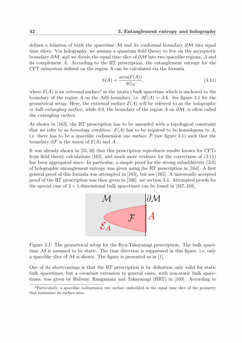
42 3. Entanglement entropy and holography

defines a foliation of both the spacetime M and its conformal boundary ∂M into equaltime slices. Via holography, we assume a quantum field theory to live on the asymptoticboundary ∂M, and we divide the equal time slice of ∂M into two spacelike regions, A andits complement A. According to the RT prescription, the entanglement entropy for theCFT subsystem defined on the region A can be calculated via the formula

S(A) =area(E(A))

4GN

, (3.11)

where E(A) is an extremal surface2 in the (static) bulk spacetime which is anchored to theboundary of the region A on the AdS boundary, i.e. ∂E(A) = ∂A. See figure 3.1 for thegeometrical setup. Here, the extremal surface E(A) will be referred to as the holographicor bulk entangling surface, while ∂A, the boundary of the region A on ∂M, is often calledthe entangling surface.

As shown in [163], the RT prescription has to be amended with a topological constraintthat we refer to as homology condition: E(A) has to be required to be homologous to A,i.e. there has to be a spacelike codimension one surface F (see figure 3.1) such that theboundary ∂F is the union of E(A) and A.

It was already shown in [55, 56] that this prescription reproduces results known for CFTsfrom field theory calculations [162], and much more evidence for the correctness of (3.11)has been aggregated since. In particular, a simple proof for the strong subadditivity (3.6)of holographic entanglement entropy was given using the RT prescription in [164]. A firstgeneral proof of this formula was attempted in [163], but see [165]. A universally acceptedproof of the RT prescription was then given in [166], see section 3.4. Attempted proofs forthe special case of 2 + 1-dimensional bulk spacetimes can be found in [167,168].

Figure 3.1: The geometrical setup for the Ryu-Takayanagi prescription. The bulk space-time M is assumed to be static. The time direction is suppressed in this figure, i.e. onlya spacelike slice of M is shown. The figure is presented as in [1].

One of its shortcomings is that the RT prescription is by definition only valid for staticbulk spacetimes, but a covariant extension to general cases, with non-static bulk space-times, was given by Hubeny, Rangamani and Takayanagi (HRT) in [169]. According to

2Particularly, a spacelike codimension two surface embedded in the equal time slice of the geometrythat minimises its surface area.

3.2 Holographic entanglement entropy 43

this prescription, in order to holographically calculate the entanglement entropy of thesubsystem of the boundary CFT defined on a spacelike codimension one region A of theboundary ∂M, one searches for bulk surfaces E(A) that are anchored to ∂A and satisfythe homology constraint as before, but now extremise the area. Then, out of all surfacesthat satisfy these conditions, the one with minimal area is chosen, and the entanglemententropy is calculated as

S(A) = minXarea(E(A))

4GN

for X = E(A) : ∂E(A) = ∂A, ∃F s.t. ∂F = E(A) ∪ A. (3.12)

The reason that the HRT prescription searches for curves extremising the area is the fol-lowing [169]: In the RT prescription, the bulk entangling curves are by definition embeddedin a spacelike time slice, and on this spacelike slice a unique minimal area surface shouldexist. In the covariant case however, the length of a spacelike curve for example can alwaysbe made arbitrarily small by deforming it closer and closer to a piecewise null curve. Theminimisation of the area in a Lorentzian background will hence not yield a well-definedspacelike surface. This is why in the HRT prescription, one first constructs the set of allwell-defined spacelike extremal surfaces, and then takes the minimal area surface in thisset.

As remarked in [170,171], the homology constraint has to be refined for the covariant pre-scription (3.12), e.g. by requiring that the codimension one surface F has to be spacelike.In the RT approach, this is the case by construction. In [64], it was discussed that the bulkentangling curves should satisfy certain causality constraints, and that this is automati-cally the case in the HRT prescription when the null energy condition is satisfied. Thesecausality conditions will play a major role in our discussion of entanglement entropy inhigher curvature theories, where we show that they are not automatically satisfied even inphysical background spacetimes, see section 4.

We will end this section by showing a very simple example of the calculation of entan-glement entropy using these holographic methods that was originally already presentedin [55]. Specifically, we will take 2 + 1-dimensional Poincare AdS (2.11) as the backgroundspacetime, and we will be interested in calculating the entanglement entropy of a boundaryinterval A defined to be a subset of the equal time slice τ = 0 and ranging from x = −∆x/2to x = +∆x/2. The bulk spacetime is static and the equal time slice τ = 0 is the Euclideanhyperbolic space

ds2 =L2

z2(dx2 + dz2). (3.13)

It is well known that the geodesics in this space are half-circles, and consequently thebulk-entangling surface needed to calculate the entanglement entropy can be given in a

44 3. Entanglement entropy and holography

simple non-affine parametrisation

z(s) =∆x

2sin(s), (3.14)

x(s) =∆x

2cos(s), (3.15)

with s ∈]0, π[. See figure 3.2 for an illustration of the geometric setup. By (3.11), theentanglement entropy will be defined by the area of this codimension two hypersurface,which is in case of such a one-dimensional curve only its length. Strictly speaking, thislength will be infinite due to the contribution of the part of the curve near the boundaryand we hence have to impose a cutoff at z = ε. As explained in section 2.3.3, this cutoffacts as an IR regulator for the bulk theory (regulating infinite volume effects), but as a UVregulator in terms of the boundary CFT. Using (3.11), the entanglement entropy is then

S =L

4GN

π−arcsin( 2ε∆x)∫

arcsin( 2ε∆x)

ds

sin(s)≈ c

3log

(∆x

ε

)+ ... , (3.16)

where ... stands for terms of higher order in ε∆x

and we used the result (2.33) to expressGN in terms of the central charge c. As expected, (3.16) reproduces the field theory resultof [162].

Figure 3.2: Geometric setup for the calculation of entanglement entropy of an intervalA = [−∆x

2, ∆x

2]. In the hyperbolic space (3.13), the spacelike geodesics are half-circles.

3.3 Black hole entropy and thermofield double states

As we can clearly see by comparing equations (2.1), (3.11) and (3.12), the holographicprescription for calculating entanglement entropy is a generalisation of the Bekenstein-Hawking formula for black hole entropy. Indeed, we can see that in the AdS/CFT cor-respondence the entropy of a static bulk black hole can be calculated as entanglement

3.3 Black hole entropy and thermofield double states 45

entropy. To do so, we have to distinguish two possible cases.

In the first case, we are working in an asymptotically Poincare black hole background, wherethe event horizon extends infinitely in the spacelike directions xµ. When we then calculatethe entanglement entropies of certain boundary systems (e.g. infinite strips) A(R) withsize R, and take the limit R→∞, we find that the corresponding holographic entanglingsurfaces in the bulk approach the event horizon more and more closely, see figure 3.3.For example, the generalisation of (3.16) to the background-spacetime given by the BTZblack hole [130, 131] with temperature T will play an important role in chapter 6 andreads [55,162]3

S =c

3log

(1

πεTsinh (πRT )

). (3.17)

Apart from the divergence ∼ log(ε) caused by the near-boundary part of these surfaces,which can be subtracted, the entanglement entropy will then be dominated by the in-creasing parts of the surfaces that are close to the horizon. For large R, the renormalisedentanglement entropy Sren can then be approximated by the area of the part of the curveEA(R) which is near the event horizon, or equivalently by the area of A(R) (measured atthe boundary) times the entropy density of the event horizon times some constant. Inthe limit R → ∞ the entanglement entropy hence reproduces the black hole entropy. Wealso see that in this limit the entanglement entropy becomes extensive, as expected for athermodynamic entropy. For example, in the limit R→∞ equation (3.17) yields

Sren ≈c

6πTR. (3.18)

These considerations will later become very useful in our study of entanglement entropyand impurity entropy in the Kondo effect, see chapter 6.

Figure 3.3: Typical holographic entangling surfaces for three boundary regions A(Ri) withsizes R1 < R2 < R3. With increasing size, the surfaces approach the event horizon closerand closer.

In the second case we deal with black holes in asymptotically global AdS, where theboundary is compactified to a (hyper-) sphere. The analogous situation to the first case

3With ∆x in (3.16) renamed to R in this context.

46 3. Entanglement entropy and holography

is a bit more complicated here, as bulk entangling curves still tend to approach the eventhorizon, but due to the finiteness of the boundary volume, the limit R → ∞ is now notpossible anymore. To investigate this case more closely, we should consider the conformaldiagram of a static asymptotically AdS black hole as it is sketched in figure 3.4. Outside ofthe event horizons, this spacetime is static, and hence equal time slices can be constructed.In such cases, as we have seen in section 3.2, we can calculate entanglement entropyholographically using the Ryu-Takayanagi prescription4. The corresponding holographicentangling surfaces are then extremal surfaces on the geometry defined by the equal timeslice, which is known as an Einstein-Rosen (ER) bridge or also Euclidean wormhole. Seefigure 3.5 for a sketch of the geometry of such an equal time slice.

Figure 3.4: Conformal diagram for a static asymptotically AdS black hole. The spacetimehas two boundaries, with CFTs 1 and 2 living on it. The flow of the (asymptotically)timelike Killing vector field ∂t is indicated with arrows. The event horizons (diagonallines) are Killing horizons, and the bifurcation surface B is defined to be the locus wherethe Killing vector field vanishes. An equal time slice with respect to the Killing field isa straight line through the center of this diagram, shown as a dotted line. The figure ispresented as in [1].

Assume we start with a subregion A of CFT1 which has a small angular extend ∆φ on theboundary sphere.5 The corresponding bulk entangling surface used in the RT prescriptionwill then be of the qualitative form of C in figure 3.5. As ∆φ grows beyond π, this willsmoothly transform into a hypersurface of the shape D, which increasingly approaches thebifurcation surface B, which is the equal time slice of the black hole event horizon. But nowwe have to take into account that according to the RT prescription, the bulk entanglingsurface need not necessarily be connected. Then, for ∆φ→ 2π, there are two possibilitiesfor extremal bulk surfaces that satisfy the homology constraint and are anchored at ∂A onthe boundary. One possibility is the surface D sketched in figure 3.5, the other possibilityis that the entanglement entropy is described by the union of the curves B and C.6 Note

4Assuming that the boundary subsystem in question is also defined on an equal time slice.5This is a generalisation of the size scale R that we used for the case of a flat boundary.6For the moment, we ignore surfaces of the type A, i.e. closed surfaces wrapping around the black hole

event horizon. In Einstein-Hilbert gravity, these are excluded by the null energy condition [172].

3.3 Black hole entropy and thermofield double states 47

that C alone would not satisfy the homology constraint with respect to the boundaryregion A. According to the RT prescription, the entanglement entropy is given by theextremal surfaces with smallest area, subject to the correct boundary conditions and thehomology constraint. Hence, as ∆φ is increased from 0 to 2π, there will generically be atransition from the entanglement entropy being defined by one surface for small ∆φ to theentanglement entropy being defined by the union of a surface anchored at the boundaryand the bifurcation surface B for large ∆φ.7 Especially, we see that if we take the limitB → 0 such that the subregion A encompasses the entirety of the right boundary, whereCFT1 lives, the (renormalised) entanglement entropy is given by the area of the bifurcationsurface B,8 i.e. the area of a slice of the event horizon. This means that the two CFTs onthe two boundaries of the eternal black hole are entangled, and the entanglement entropybetween them is exactly the Bekenstein-Hawking entropy (2.1), or in the nomenclature ofthis section [169,170]

S =area(B)

4GN

. (3.19)

This implies that after tracing out the degrees of freedom of CFT2, CFT1 is left in athermal state with density matrix (3.1) and an entropy (3.19) that could be interpreted asthermal entropy from a viewpoint of the CFT1, but that is an entanglement entropy froma viewpoint that takes into account both CFT1 and CFT2.

The remaining question is: What is the total state of CFT1 and CFT2 dual to the eternalblack hole? The answer was given by Maldacena in [173], where he proposed that in theweak form of the AdS/CFT conjecture, the total state of the two CFTs dual to the largestatic eternal black hole9 is the (pure) thermofield double state

|Ψ〉 =1√Z(β)

∑i

e−12βEi |Ei〉1 |Ei〉2 , (3.20)

where the notation is similar to equation (3.1) and the states |Ei〉1/2 are energy eigenstatesof CFT1/2 respectively. Starting from this state (3.20), it is then easy to take the traceon the Hilbertspace of CFT2 and find that the reduced density matrix for CFT1 will bethe thermal one (3.1). This pure thermofield double state describing two entangled CFTsis hence analogous to the EPR state (3.8) describing two entangled spins. This is onemanifestation of the ER=EPR proposal mentioned in section 1.

The fact that the entropy of the bulk black hole holographically describes the entropy ofthe CFT on one of the boundaries, described by the density matrix of a thermal state, wasalready derived without the use of entanglement entropy in [27, 174]. To understand thisresult, we should note that for a thermal canonical ensemble, the CFT thermodynamics

7This also leads to the phenomenon of entanglement plateaux studied in [170].8As area(C)→ 0 in this limit.9The AdS-black hole is assumed to be large compared to the AdS-scale in order to have positive specific

heat and be the dominant contribution to the canonical thermodynamic ensemble [173].

48 3. Entanglement entropy and holography

Figure 3.5: Left: The geometry of an Einstein-Rosen bridge, which is the equal time slicesignified in figure 3.4 by a dotted line. Several types of possible curves on such a timeslice are shown as A,B, C,D. B is the bifurcation surface, which is the throat of thewormhole, where the circumference of the geometry is the smallest. Curves of the type ofA are usually not possible in Einstein-Hilbert gravity [172], but will play a role in highercurvature theories, see chapter 4. Right: A similar sketch, showing only the spacetimeregion between the bifurcation surface and the right boundary (divided into regions A andB), where CFT1 is assumed to live via the holographic duality. The figures are presentedas in [1].

can be inferred from the (canonical) partition function Z(β) = Tr[e−βH

]. Then, one can

define quantities such as the free energy βF = − logZ(β) and the field theory entropySCFT = β2∂βF . Holographically, the weak form GKPW formula (2.60) equates the CFTpartition function with the saddle point approximation of the gravity partition function,i.e.

Z = e−SE(β), (3.21)

where SE is the Euclidean on-shell action of the dominant bulk saddle for a given temper-ature. This dominant saddle will be a black hole, at least for large temperatures [27,174].It then follows that βF = S and the CFT thermal entropy can be calculated from thegravity on-shell action to be [27,174]

SCFT = β2∂β

(1

βS). (3.22)

This on-shell action approach to black hole entropy reduces to the area formula (3.19)[27,174], and hence we find

SCFT = SBH =area(B)

4GN

, (3.23)

reproducing the result derived via entanglement entropy above.

3.4 The replica method 49

3.4 The replica method

So far, we have seen concrete examples of how entanglement entropy can be calculated forsimple spin-systems, as well as in holographic contexts. To gain a deeper understandingof entanglement entropy in field theory terms, in this section we present a brief overviewover the replica trick or replica method. Although this method has been developed in thecontext of spin glasses (see e.g. [175]), we will in this section follow the outline presentedin [162] as well as the summary of [52].

The first step towards understanding the replica method is to write the entanglemententropy (3.4) in the form

SA = −TrA[ρA log ρA] = − limn→1

∂

∂nTr [ρnA] . (3.24)

SA can hence be calculated by the detour of calculating Tr [ρnA] for any integer n > 1,analytically continuing to general n > 1 and taking the appropriate limit [162]. Thevirtue of the replica method is that the quantity Tr [ρnA] can be calculated via path integralmethods. For simplicity, we will now restrict our discussion to Euclidean two-dimensionalquantum field theories, with a Euclidean time coordinate t and a space coordinate x. Wewill also assume this Euclidean space to be simply a cylinder where the time is compactifiedwith a period β = 1/T .

The path integral can now for example be used to calculate transition probabilities betweentwo states at different Euclidean times, or the thermal partition function

Z =

∫D[φ]

∣∣t∼t+β e

−SE , (3.25)

where we have collectively called the fields of the theory φ, and the Euclidean actionSE. The integration is over all field configurations that satisfy the appropriate periodicityconditions for finite temperature. In the following, we consider the case where a subsystemA is defined to be an interval on the t = 0 line of the Euclidean space. The reduced densitymatrix ρA then reads [162]:

ρ =1

Z

∫D[φ]

∣∣t∼t+β for x∈A

∏x∈A

δ(φ(x, 0+)− φ′(x))∏x∈A

δ(φ(x, 0−)− φ′′(x)) e−SE . (3.26)

The interpretation of this formula is that the periodicity conditions are only imposedon the fields outside of A, while in the subsystem A we impose the boundary conditionφ′(x) at an infinitesimal time-step to the future and φ′′(x) at an infinitesimal time step tothe past. This implements the tracing out of the complement A (ρA = TrA[ρ]), and thefunctions φ′ and φ′′ can be seen as indices of the reduced density matrix, (ρA)φ′φ′′ . It is nowstraightforward to understand how the quantity Tr [ρnA] can be calculated by introducingn copies, also called replicas, of the manifold on which the QFT lives. See figure 3.6 for an

50 3. Entanglement entropy and holography

illustration. One simply sews together the n copies of the spacetime along the subsystemA in a cyclic way, always identifying the state on the 0+-line of replica i with the state onthe 0−-line of replica i+ 1. Taking the overall trace is then implemented by identifying thestate on the 0+-line of replica n with the state on the 0−-line of replica 1.

Figure 3.6: An illustration of the replica method, here for the case n = 3. The subsystemA is seen as a cut in the space on which the field theory lives, and n replicas of the spaceare sewn together along this cut in a cyclic manner.

This means that we are effectively working with an n-sheeted Riemann surface Rn, andthe reduced density matrix is related to the partition function Zn(A) of the QFT on thisRiemann surface via the equation [162]

Tr [ρnA] =Zn(A)

Zn. (3.27)

Thus, the replica trick suggests a possible way to calculate entanglement entropy by cal-culating the expressions Zn(A) for integer n > 1. Unfortunately, this is still a non-trivialtask in general, but analytic results such as (3.17) can be derived for two dimensionalCFTs [162]. We will not go into the details of this, instead we will in the rest of this sec-tion give a brief overview over how the replica trick was used for a holographic derivationof the Ryu-Takayanagi prescription (3.11) in [166], see also [163, 165, 167, 168] for earlierwork. To do so, we will follow the overviews presented in [52] and [62].

The idea behind the proof given in [166] is to extend the replica trick into the bulk space-time. Specifically, for the case of n replicas, there should be a bulk spacetime Bn such thatRn is the conformal boundary of this bulk spacetime, and Bn is a solution to Einstein’sequations. The generalisation of (3.21) then reads

Zn(A) = e−SE, bulk(Bn). (3.28)

For integer n, the boundary manifold Rn has a cyclic Zn symmetry (of shifting the replicasi → i + m modulo n), and this is conjectured to be also the case for Bn [166]. The set ofpoints that are invariant under this Zn symmetry is very interesting: On the boundary Rn,

3.4 The replica method 51

these points will be the boundary ∂A of the subsystem A, i.e. the endpoints of the cut alongwhich the replicas are sewn together. In the bulk spacetime Bn, the set of fixed points willform a codimension two surface that reaches to the boundary Rn and is anchored there at∂A. For simplicity, we refer to this set of fixed points as E(A), as in the limit n→ 1 it willbecome the holographic entangling surface defined in section 3.2. Instead of Bn, it is nowuseful to look at the orbifold

Bn = Bn/Zn. (3.29)

The hypersurface E(A) is then the locus of a conical defect in Bn. Excluding boundaryterms of the action at the locus of this conical defect, one can then write SE, bulk(Bn) =

nSE, bulk(Bn) [62, 166]. Furthermore, as Tr[ρ] = 1, (3.24), (3.27), (3.28) and (3.29) can beused to derive [62,166]

SA = − limn→1

∂nTr [ρnA] = − limn→1

∂n log Tr [ρnA] = limn→1

1

1− nlog Tr [ρnA] (3.30)

= limn→1

n

n− 1

(SE, bulk(Bn)− SE, bulk(B1 = B1)

)= lim

n→1∂nSE, bulk(Bn) (3.31)

As shown in [62,166], the metric in the vicinity of this hypersurface can be written as

ds2 = ρ−2ε(dρ2 + ρ2dτ 2

)+(hij + 2k

(α)ij x

α)dyidyj + ..., (3.32)

where the yi are coordinates along E while xα ∈ ρ, τ ∼ τ + 2π are polar coordinatesin the plane normal to the conical defect surface. The conical defect is parameterised byε = 1− 1/n, and the k

(α)ij are extrinsic curvature tensors, see appendix A. The terms ... are

terms in higher order of ρ. The virtue of this approach of introducing Bn and the metric(3.32) is that this setup can easily be generalised to non-integer n.

As shown in [166], imposing Einstein’s equations to be satisfied by the metric (3.32) leads,in the limit n→ 1, to the condition

k(α)ii = 0, (3.33)

i.e. the traces of the extrinsic curvature tensors have to vanish. This means nothing elsethan that the surface E(A) has to be an extremal surface10, as expected from the holo-graphic prescriptions discussed in section 3.2. This is a very important result, as in chapter4 we will be concerned with locating the extremal surfaces that define entanglement en-tropy in higher curvature theories. Furthermore, a detailed analysis of the terms arisingin the action SE, bulk(Bn), which will not be repeated here for the sake of brevity, confirmsthat the correct entropy functional is indeed (3.11) [166].

As we have seen in this chapter, entanglement entropy is a widely studied topic in theAdS/CFT literature and it would lead too far to summarise here all the ways in which

10In the sense of extremising its area.

52 3. Entanglement entropy and holography

the study of entanglement entropy has lead to new insights into the nature of holography.Instead, we will devote the remaining chapters of this thesis to highlighting the contribu-tions that the author made to the understanding of holographic entanglement entropy incertain contexts. In chapter 4, we study how prescriptions for calculating entanglemententropy in bulk theories with higher curvature terms in the action will be constrained byrequirements of causality. In chapters 5 and 6 we will study bottom-up models of boundaryCFTs (BCFTs), and how entanglement entropy can be used in such models to define defectentropy and monitor the behaviour of this quantity under holographic RG flows.

Chapter 4

Entanglement entropy in highercurvature theories

4.1 Introduction

In the following chapter, we will present the results obtained by the present author in [1]. Insection 3.3 we have seen that in AdS/CFT, the entropy of eternal black holes is interpretedas the entanglement entropy between two CFTs living on the two AdS boundaries. While,as we discussed in section 2.1.1, the entropy of a black hole in Einstein-Hilbert gravityshould be given by the Bekenstein-Hawking formula (2.1), the generalisation of this formulato gravitational theories with higher curvature terms in the action (e.g. R2, RµνR

µν etcetera) was given by Wald and others in [57–59]. There, it was derived that for a stationaryblack hole in a higher curvature theory with action

S =1

16πGN

∫dd+1x

√−gL, (4.1)

the black hole entropy can be calculated by evaluating a certain entropy functional on thebifurcation surface B (see section 3.3) of the black hole [57–59]:

SWald =−1

8GN

∫B

dd−1y√γ

∂L∂Rαβγδ

εαβεγδ. (4.2)

Here εαβ is called the binormal and, using εαβεαβ = −2, (2.1) follows as the special casefor Einstein-Hilbert gravity [57–59]. Now as we have seen in sections 3.2 and 3.3 theholographic prescriptions for the calculation of entanglement entropy can be consideredto be a straightforward generalisation of the entropy formula (2.1) for black holes. Willholographic entanglement entropy calculations in higher curvature bulk theories then be astraightforward generalisation of (4.2)? The answer is both yes and no. “Yes” because, as

54 4. Entanglement entropy in higher curvature theories

explained in section 3.3, the prescription for calculating holographic entanglement entropyhas to reproduce the correct black hole entropy. “No” because the necessary generalisationof (4.2) will not be straightforward. In the derivation of [57–59], there where severalpossible ambiguities that did not matter as the corresponding terms always vanish whenevaluated on a bifurcation surface B [176]. Nevertheless, holographic entanglement entropyin higher curvature theories has been an active field of research in holography, startingalready with [163,176,177] for specific theories, continuing with [60,61] for general theorieswith higher curvature terms of order R2 and reaching the most general result up to datewith [62,63]. Specifically, for a higher curvature theory of the form

S =1

16πGN

∫dd+1x

√−g[R + 2Λ + aR2 + bRµνR

µν + cRµναβRµναβ

], (4.3)

the entropy functional proposed in [60–63] based on replica methods similar to the argu-ments discussed in section 3.4 reads:

SEE(Σ) =1

4GN

∫Σ

dd−1y√γ

[1 + 2aR + b

(R‖ −

1

2k2

)+ 2c

(R‖‖ − Tr(k)2

)]. (4.4)

This indeed reduces to (4.2) when evaluated on a black hole bifurcation surface [60–63].For an explanation of the notation used in this formula, see appendix A.1.

The derivations done in [60–63] are a generalisation of the calculations of [166] (see section3.4) to higher curvature theories, and as such are quite involved. However, just like the endresult of [166] was the simple Ryu-Takayanagi prescription (3.11), the general prescriptionhow to calculate holographic entanglement entropy using the functional (4.4) is thoughtto be simply a generalisation of the RT and HRT prescriptions studied in section 3.2. Ac-cording to [62], in order to calculate the entanglement entropy of a boundary subregion A,one has to find a codimension two spacelike surface extremising the functional (4.4) andsatisfying the same boundary conditions as the curve E(A) in the RT and HRT prescrip-tions, i.e. ∂Σ = ∂A and the homology condition. If several extremal surfaces Σ satisfyingthese conditions exist, one would take the one yielding the smaller entropy (4.4) to be theone defining the physical holographic entanglement entropy.

In this chapter, however, we will apply this prescription to two different physical theoriesand find that there are special situations in which this prescription yields extremal surfacesΣ that satisfy all conditions described above and give the lowest entropy, but that shouldnot be considered to be the correct physical surface defining entanglement entropy. Inparticular, following the thoughts of section 3.3 we will look for hypersurfaces extremisingthe functional (4.4) which are not anchored to the asymptotic boundary, but which areclosed and wrap around a black hole, such as curve A in figure 3.5. If such a curve wasto define entanglement entropy between the two CFTs on the boundaries of an eternalblack hole, this would mean that the entanglement entropy (SEE(A)) would no longer beequivalent to the black hole entropy (SEE(B) = SWald), violating the expectations fromsection 3.3 and, e.g., [27,174]. In section 4.4 we will show that the imposition of additionalcausality constraints serves to distinguish physical from unphysical extremal surfaces.

4.2 New massive gravity 55

4.2 New massive gravity

The first higher curvature theory that we are going to work with is new massive gravity(NMG) which is a toy model of gravity in 2 + 1 dimensions that was proposed in [178,179]and studied in the holographic context in [180–187]. The action is written as

S =1

16πGN

∫d3x√−g

[σR− 2λm2 +

1

m2

(RµνR

µν − 3

8R2

)]. (4.5)

Here the mass parameter m2 may take any sign, λ is a cosmological constant parameterand σ = ±1 allows us to choose the sign of the Einstein-Hilbert term. The parameterspace of this theory is quite complicated and we will now summarise the most importantaspects of it following [179].

First of all, we are interested in whether the corresponding equations of motion allow forAdS solutions. This can be shown to be the case if the AdS radius L satisfies the equation

1

L2= 2m2

(σ ±√

1 + λ), (4.6)

i.e. only for λ ≥ −1 [179]. Unfortunately, NMG is known to be plagued by several problemsthat cast doubt on its validity as a physical theory1. First of all, ghosts, i.e. negative energygravitons, are only absent when

m2(Λ− 2m2σ) > 0 (4.7)

where we defined Λ = −1/L2 [179]. As a second constraint, we have to impose theBreitenlohner-Freedman bound [179,197]

−2m2σ ≥ Λ. (4.8)

Furthermore, one can determine the central charge of the assumed CFT dual of NMG tobe [179,198]

c =3L

2GN

(σ +

1

2m2L2

), (4.9)

which should ideally be positive. Unfortunately, (4.7) and the condition c ≥ 0 in (4.9)are mutually exclusive. An overview over the parameter space of NMG and the differentconditions discussed above is given in figure 4.2 at the end of this subsection.

1Nevertheless, as a model of gravity in 3 dimensions with propagating degrees of freedom this theoryhas received much attention, just like the (similarly problematic) topologically massive gravity [188, 189].In the recent years, much effort has been invested into two theories that are hoped to be just as interesting,yet in many aspects physically better behaved. These are zwei-dreibein gravity [190–193] and minimalmassive gravity [194–196]. Unfortunately, these theories are not of the form (4.3) and hence (4.4) does notapply. How to calculate entanglement entropy in these theories seems to be an open problem.

56 4. Entanglement entropy in higher curvature theories

As AdS3 is a solution to NMG for certain parameters, the same holds for the BTZ blackhole [130, 131] which is constructed via global identifications of an AdS3 background. InSchwarzschild like coordinates, the line element for the non-rotating case reads2

ds2 = −(−M +

r2

L2

)dt2 +

(−M +

r2

L2

)−1

dr2 + r2dφ2. (4.10)

The event horizon is obviously located at rH = L√M . The entropy of this black hole in

NMG can then be shown to be [179,198]

SBTZ =2πrH4GN

(σ +

1

2m2L2

). (4.11)

Positivity of the black hole entropy is hence tied to positivity of the central charge (4.9).

As shown in [199], in NMG the functional (4.4) takes the form

SEE =1

4GN

∫dτ√gττ

[σ +

1

m2

(R‖ −

1

2k2 − 3

4R

)], (4.12)

where√gττ =

√gµν

dxµ

dτdxν

dτand τ is the parameter along the curve.3 In [1] we studied

curves extremising this functional both anchored at the boundary and closed in the bulk.In this thesis, we will for simplicity only present the closed curve solutions in the following.4

As we have seen in section 3.3, such closed extremal curves should holographically describethe entanglement between the two CFTs living on the two boundaries of an eternal blackhole.

In order to find such extremal curves, we would usually have to vary the functional (4.12)in order to obtain equations of motion, just as the geodesic equations can be found by vary-ing the length functional

∫dτ√gττ . Unfortunately, the resulting equations of motion are

notoriously complicated. To simplify things, on can make something like a minisuperspaceansatz, i.e. assume that the solutions will have certain symmetry properties, plug a cor-responding ansatz for the curve into the functional (4.12) and obtain simplified equationsof motion by varying with respect to the remaining functions respectively the remainingparameters of the ansatz. The solutions that are obtained this way can then be pluggedinto the full equations of motion (i.e. using a computer program like Mathematica) to bechecked for their validity. So to be specific, we will make two assumptions about potentialclosed surfaces extremising (4.12) in a BTZ background (4.10). First of all, as the space-time is static outside of the horizon, we will assume our putative extremal surfaces to be

2In this thesis we will restrict ourselves to the nonrotating BTZ case. Rotating BTZ black holes andLifshitz black holes in NMG have also been briefly investigated in [1].

3As NMG is a theory in three bulk dimensions, the codimension two hypersurfaces that define entan-glement entropy are one-dimensional curves in this case. See also the example in section 3.2.

4Besides [1], extremal curves anchored at the boundary have also been studied in NMG in [186,200,201].In [200], special boundary conditions were proposed to restrict the holographic entangling curves. In [201],field redefinitions where used to obtain the correct physical extremal surfaces.

4.2 New massive gravity 57

embedded in constant time slices, i.e. t(τ) = const. Also, we will assume these curves tobe invariant under translations generated by the angular Killing vector field ∂φ, hence ouransatz is r(τ) = const., φ(τ) ∝ τ .

One technical problem that we encounter immediately is that the Schwarzschild coordinatesused in (4.10) are not valid on the event horizon of the black hole. This problem could easilybe solved by going to the Kruskal coordinates for the BTZ black hole [130, 131], yet thesemake computations significantly more complicated. For the sake of a concise presentation,just as in [1] we will hence continue to work in Schwarzschild coordinates. All our resultscan be, and were, checked for correctness by calculations in Kruskal coordinates, both inthe Lorentzian and Euclidean BTZ metric where applicable.

As, however, the Schwarzschild coordinates do not cover the bifurcation surface B, definedby

rB = rH = L√M, (4.13)

we have to be careful not to overlook this curve as an extremal curve of the entropyfunctional (4.12). In fact, the bifurcation surface of a black hole extremises not only thearea functional, but in fact any physical functional like (4.4). The reason for this lies inthe symmetries of the black hole spacetime, see figure 3.4 again. We expect that if somefunctional is evaluated on a given surface in the black hole spacetime, then if we movethis surface along the flow of the Killing vector field ∂t, the resulting surface yields thesame value when the functional is evaluated on it. But the bifurcation surface B is thesurface on which the two Killing horizons in figure 3.4 cross and hence it is the set offixed points under the flow of the Killing vector field. Also, the maximally extended staticblack hole spacetimes are time inversion symmetric as well as symmetric under exchangeof the left and the right side. These symmetries of a conformal diagram as figure 3.4 implythat the bifurcation surface B will always be a local saddle point to any functional of theform (4.4) on a static black hole background. This means that, if no other closed solutionsdo exist, the entanglement between the two CFTs on the two boundaries of the eternalblack hole will always be given by the black hole entropy (4.11), as the functional (4.4)by definition reduces to Wald’s result (4.2) on a bifurcation surface. This would be thephysically expected result.

The problem that we will be concerned with in this chapter, and that was studied in [1],is that generically functionals of the form (4.4) do allow for additional closed extremalcurves in black hole backgrounds. The first example that we encounter is NMG, whereupon inserting our symmetric ansatz for a potential closed surface the functional (4.12)takes the form

S ∝ σr +M

2m2r(4.14)

for a closed curve of radius r. This means that apart from the bifurcation surface (4.13),

58 4. Entanglement entropy in higher curvature theories

we find a closed curve extremising (4.12) at radius

r =

√M

2σm2. (4.15)

Comparing this to the event horizon located at r = rH (4.13), we see that this additionalextremal surface will be outside of (or exactly on) the event horizon for σm2L2 ≤ 1

2, which

is precisely the Breitenlohner-Freedman bound (4.8). For σm2L2 < 0, this solution is illdefined and no additional extremal surfaces exist.5 Due to the symmetry generated by thetimelike Killing vector field ∂t (see figure 3.4), these additional curves do not appear assolitary codimension two surfaces, but they foliate codimension one hypersurfaces invariantunder flows of ∂t. Depending on σm2L2, we hence find one of the four possible configura-tions shown in figure 4.1. In figure 4.2 we compare these different possible configurationswith the restrictions imposed on NMG by the Breitenlohner-Freedman bound (4.8), thecondition of unitarity (c ≥ 0) and the absence of ghosts (4.7). As already said earlier, thelatter two conditions are mutually exclusive, but it is interesting to point out that noneof the possible pathologies of NMG seems to be in a one to one correspondence with theappearance of additional extremal surfaces.

Of course, according to the RT and HRT prescriptions, we would be required to takethat extremal curve to define the entanglement entropy between the two CFTs on the twoboundaries that yields the lowest value for the entanglement entropy. By definition, theentropy functional (4.12) evaluated on the bifurcation surface B will yield the Wald entropy(4.11). In contrast, the additional surface (4.15) yields an entropy

Sa =2πσ

4GN

√2M

σm2. (4.16)

In the parameter regime where (4.15) is a real solution, we then find |SBTZ | ≥ |Sa| withequality for σm2L2 = 1/2, where the additional extremal surfaces are slices of the eventhorizon. This is depicted as case c) in figures 4.1 and 4.2.

For positive black hole entropy SBTZ (equivalent to positive central charge (4.9)), the RTand HRT like prescriptions for higher curvature theories discussed at the beginning of thischapter would then suggest that the entanglement entropy between the two CFTs on thetwo boundaries is in fact not given by the black hole entropy SBTZ , but by the entropy Saassociated with the additional extremal closed curve. On physical grounds, this would be avery counterintuitive result, as it would mean that the black hole entropy (calculated on thebifurcation surface via Wald’s formula (4.2)) would no longer be the entanglement entropybetween the two CFTs. In fact, we will see in section 4.4 that the additional extremalsurfaces found in this section have to be discarded for reasons of causality. Yet beforestudying these causality conditions, we will leave the topic of NMG and study anotherhigher curvature theory instead, namely the well known Gauss-Bonnet gravity. This is

5Remember that we formally allow m2 to have any sign, but L2 is positive.

4.3 Gauss-Bonnet gravity 59

Figure 4.1: Four possible configurations of additional extremal surfaces (4.15), dependingon the value of σm2L2. The bifurcation surface B is always an extremal curve of theentropy functional. a): σm2L2 < 0, no additional closed extremal curves exist in the BTZgeometry. The flow of the Killing vector field ∂t is sketched by arrows. b): 0 ≤ σm2L2 < 1

2,

and the additional curves lie outside the event horizon. They are spacelike slices of atimelike hypersurface invariant under flows of ∂t. c): σm

2L2 = 12, the additional surfaces

are slices of the event horizon. d): σm2L2 > 12, the additional extremal surfaces are inside

of the event horizon. The figure is presented as in [1].

worthwhile as, as stated above and shown in figure 4.2, NMG is plagued by numerouspathologies. We will show that Gauss-Bonnet gravity, although being much better behavedas a physical theory than NMG, will also give rise to additional extremal closed surfacesthat pose a problem for the calculation of entanglement entropy. We hence expect thatproblems of this kind for prescriptions for the calculation of entanglement entropy basedon functionals like (4.4) may to a certain extend be generic to higher curvature theories.

4.3 Gauss-Bonnet gravity

Gauss-Bonnet gravity is a special case of Lovelock gravity [202] (see also [203]) and itsaction in five dimensions can be written as [177]

S =1

16πGN

∫d5x√−g

[R +

12

L2+ λ

L2

2

(RµναβR

µναβ − 4RµνRµν +R2

)]. (4.17)

This corresponds to the special choice of the parameters a, b, c in (4.3) such that the actionand the corresponding equations of motion contain higher curvature terms, but can bewritten without higher derivatives of the metric [202,203]. This means that the equationsof motion for the metric are still second order, in contrast to NMG for example. Gauss-Bonnet and Lovelock theories of gravity are hence frequently studied models of highercurvature gravity in higher dimensions6 both in general gravitational physics [202,203] andAdS/CFT research [176, 177, 204, 205]. Just as it was the case for NMG, the parameterspace for Gauss-Bonnet theory (4.17) has been studied in much detail in the literature. To

6In four or less bulk dimensions, the Gauss-Bonnet term RµναβRµναβ − 4RµνR

µν + R2 would be atopological invariant.

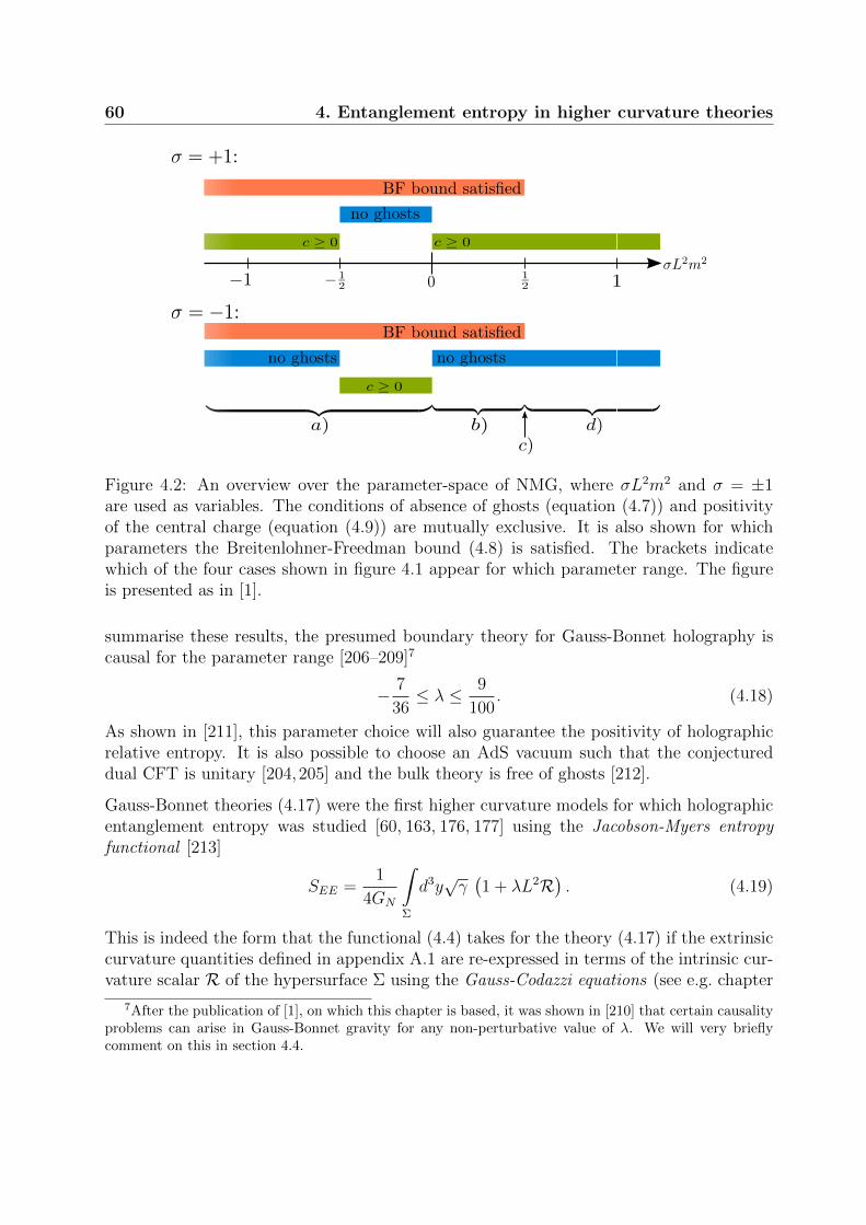
60 4. Entanglement entropy in higher curvature theories

Figure 4.2: An overview over the parameter-space of NMG, where σL2m2 and σ = ±1are used as variables. The conditions of absence of ghosts (equation (4.7)) and positivityof the central charge (equation (4.9)) are mutually exclusive. It is also shown for whichparameters the Breitenlohner-Freedman bound (4.8) is satisfied. The brackets indicatewhich of the four cases shown in figure 4.1 appear for which parameter range. The figureis presented as in [1].

summarise these results, the presumed boundary theory for Gauss-Bonnet holography iscausal for the parameter range [206–209]7

− 7

36≤ λ ≤ 9

100. (4.18)

As shown in [211], this parameter choice will also guarantee the positivity of holographicrelative entropy. It is also possible to choose an AdS vacuum such that the conjectureddual CFT is unitary [204,205] and the bulk theory is free of ghosts [212].

Gauss-Bonnet theories (4.17) were the first higher curvature models for which holographicentanglement entropy was studied [60, 163, 176, 177] using the Jacobson-Myers entropyfunctional [213]

SEE =1

4GN

∫Σ

d3y√γ(1 + λL2R

). (4.19)

This is indeed the form that the functional (4.4) takes for the theory (4.17) if the extrinsiccurvature quantities defined in appendix A.1 are re-expressed in terms of the intrinsic cur-vature scalar R of the hypersurface Σ using the Gauss-Codazzi equations (see e.g. chapter

7After the publication of [1], on which this chapter is based, it was shown in [210] that certain causalityproblems can arise in Gauss-Bonnet gravity for any non-perturbative value of λ. We will very brieflycomment on this in section 4.4.

4.3 Gauss-Bonnet gravity 61

10.2 of [105]). The fact that the entropy functional (4.4) can be expressed completely interms of intrinsic curvature quantities as in (4.19) is one of the many special properties ofGauss-Bonnet gravity.

Just as earlier for NMG, we will now try to find out whether Gauss-Bonnet gravity also al-lows for the existence of closed hypersurfaces (other than bifurcation surfaces) extremisingthe entropy functional (4.19). To begin this investigation, we will consider the backgroundspacetime gµν to be a spherically symmetric static black hole solution of Gauss-Bonnetgravity [214–217]. As the functional (4.19) is only dependent on intrinsic curvature quanti-ties, we see that the specific form of the background metric is not important at all. Supposethat the spherically symmetric background metric is given in terms of a time coordinate t,a radial coordinate r, and the angular coordinates θ, φ, ψ. Similar to the symmetric ansatzthat we made in the NMG case, we can again assume that our putative extremal surfaceΣ is extended in the angular directions and defined by a choice of r and t = const.8 Theinduced metric of Σ will hence be the one of a 3-sphere, with R = 6/r2. Consequently,(4.19) simplifies to

SEE =π2

2GN

(r3 + 6λL2r

). (4.20)

Again, just as discussed for the NMG case in section 4.2, we should not forget that bysymmetry the bifurcation surface B will always be a saddle point of the entropy functional(4.19), even if the formula (4.20) does not make this manifest due to the shortcomings ofSchwarzschild coordinates.

We easily see that the functional (4.20) indeed allows for additional extremal surfaces ifthe parameter λ is negative. These additional extremal surfaces will then be defined by

r = ra =√−2λL, (4.21)

and the entropy functional evaluated on this surface will take the value

Sa =2π2L3

GN

√−2λλ < 0 (4.22)

as λ < 0. This would be problematic, not only because the existence of additional closedextremal surfaces collides with the holographic interpretation of black hole entropy asentanglement entropy between two CFTs (as we discussed already for NMG), but alsobecause clearly no entropy should be negative. These additional extremal surfaces thatarise in RT or HRT like prescriptions (i.e. based on extremising an entropy functional) tocalculate entanglement entropy in Gauss-Bonnet gravity are hence clearly unphysical, andit is desirable to have a tool that allows to identify such unphysical solutions and discard

8Due to ∂t being a Killing vector, we expect that the value of the constant will not be important, andthat this value can indeed be shifted at will. The extremal codimension two surfaces found this way willthen define a foliation of a codimension one hypersurface invariant under the flow of the Killing vectorfield, just as it was the case for NMG. See again figure 4.1.

62 4. Entanglement entropy in higher curvature theories

them. In the discussion of the above result (4.22) we could easily invoke the argumentthat this result (and the corresponding extremal surface) are unphysical in the contextof calculating holographic entanglement entropy as the result is negative, but the readershould be reminded that this argument would not work in the NMG case studied earlier.Likewise, the problems encountered in the study of NMG (unitarity, ghosts) are absent inGauss-Bonnet gravity. In section 4.4 we will hence investigate causality arguments thatserve as a tool to rule out such unphysical extremal surfaces both in NMG and Gauss-Bonnet gravity alike, and that can easily be applied to any other higher curvature theoryin which entanglement entropy is to be studied.9

But before we do so, a few comments are in order. First of all, we should check whetherthe solution (4.21) derived via the symmetric ansatz actually satisfies the full equations ofmotion for the extremal surface that can be derived from the functional (4.19) without anyprior symmetry assumptions. Luckily, these equations of motion were explicitly workedout in [199,218–220] and take the form

X ijk(α)ij ≡

(1

2γij + λL2

(1

2γijR−Rij

))k

(α)ij = 0, (4.23)

which is the Gauss-Bonnet generalisation of (3.33). The spherical hypersurface Σ withradius (4.21) then indeed solves this equation with X ij = 0. This is an interesting contrast

to the black hole bifurcation surface, which solves this equation due to k(α)ij = 0.

As a second comment, we should point out that while the case λ < 0 is not unphysicalaccording to (4.18), it is a case that is studied much less commonly than λ > 0. This isbecause one motivation to study Gauss-Bonnet gravity models is that such higher curvatureterms appear as corrections in string theory [206,212,221]. In such a context, the parameterλ in (4.17) should then be positive and perturbatively small. Interestingly, if we had studiedbackground spacetimes with hyperbolic symmetries instead of spherical symmetries above,then we would have found R = −6/r for a symmetric ansatz and additional surfaces withradial coordinate ra =

√2λL would have appeared for positive λ.

The third and most important remark that we have to make at the end of this sectionconcerns the existence of black holes that are sufficiently small to allow for the additionalsolutions described by (4.21) to exist in the spacetime at all. In Einstein-Hilbert gravity,the singularity of the (AdS) Reissner-Nordstrom black holes is located at r = 0, and hencea spherical surface of fixed positive radius could always exist in the spacetime. Even more,by tuning the mass and charge, we could always find a black hole for which the eventhorizon would lie below any spherical surface of fixed radius. Unfortunately, this is not soeasy in Gauss-Bonnet gravity: There can be shown [216, 217, 222] to be a lower bound onthe event horizon radius for Gauss-Bonnet vacuum spherical and charged hyperbolic blackholes that coincides exactly with our result for the radius of the additional extremal surface.

9In [1] we also investigated an approach of constraining additional extremal surfaces by deriving con-straints from a conical boundary conditions method. Unfortunately, there are examples where these addi-tional constraints are too restrictive, hence we will not discuss this ansatz in this thesis.

4.4 The causal influence argument 63

Hence these additional surfaces could never exist outside of the black hole event horizon,ruling out situations of the type b) depicted in figure 4.1. Furthermore, there may even bea lower bound on the radial coordinate of the singularity, and in the vacuum case [216,217]this completely rules out our additional extremal surfaces: Not only would they have toappear below the event horizon, but also below the singularity, i.e. they are not part ofthe physical spacetime. For the charged case [222] the lower bound on the singularity isreduced sufficiently to allow the extremal surfaces derived above to appear in the spacetimeregion between singularity and outer event horizon, similar to the case d) depicted in figure4.1. Anyhow, our computations above were based only on the intrinsic curvature of theputative extremal surfaces, and hence not sensitive to the presence of a wormhole throat(as in figure 3.5) at all. Consequently, the additional extremal surfaces derived above wouldalso be problematic in global AdS space or boson star spacetimes [223, 224]10, where dueto the absence of a bifurcation surface we would expect the functional prescriptions forcalculating entanglement entropy for the boundary CFT to yield zero, corresponding to apure boundary state.

To close this section, it is interesting to note that after the publication of [1], there wherealso other papers that found unexpected phenomena in Gauss-Bonnet gravity for λ < 0[225,226]. See also [227] for an earlier study.

4.4 The causal influence argument

In this section, we will present a simple physical argument that can be applied to NMG,Gauss-Bonnet gravity and any other gravitational theory to determine certain putativebulk entangling surfaces to be unphysical. This is what we will refer to as the causalinfluence argument, presented in [64].

The gist of the causal influence argument is to avoid causal paradoxes. After all, we demanda certain quantity in the bulk (an entropy functional evaluated on a given spacelike extremalsurface) to be equal to a corresponding quantity on the boundary (entanglement entropyof a certain subsystem on the boundary). If it was possible to influence (and hence change)the bulk quantity at a time where the boundary quantity is already fixed, this would leadto a causal paradox.

Let us be more specific. Assume we are trying to calculate the entanglement entropy of aCFT subregion A using the bulk entangling curve E(A). As usual in the RT prescription,we assume that there is a well-defined notion of equal time slices, and that A is a subregionof such an equal time slice on the boundary. Without loss of generality, we assume that Alies on the t = 0 slice. If we know the CFT state at t = 0, we can calculate the value of theentanglement entropy S(A) by field theory techniques, i.e. the value is fixed at t = 0 as

10These papers only study boson stars for λ > 0, yet the authors of those papers confirmed in privatecorrespondence that similar solutions can be found for λ < 0.

64 4. Entanglement entropy in higher curvature theories

we said above. If it was possible for an observer at or arbitrarily close to the boundary tosend a signal into the bulk at a time t = δ > 0 such that this signal still reaches the curveE(A) in the bulk, this signal could, due to its backreaction on the geometry, change E(A)and hence the holographically calculated value of S(A). This would lead to the paradoxdescribed above. A first putative version of the causal influence argument could hence beformulated to demand that there should be no causal curve from the boundary region Ato the bulk entangling curve E(A). Likewise, by time reflection symmetry there shouldbe no causal curve going from E(A) to A, and as for a pure total state S(A) = S(A)(section 3.1), there should be no causal curves connecting E(A) and the complement A. Ina choice of nomenclature differing from [64], we will refer to the set of points in the bulkspacetime that are not in causal contact with a boundary region A to be the causal shadowof A. See the left of figure 4.3 for an illustration. As the extremal surfaces used in the RTprescription are calculated on the equal time slice we see that the RT prescription satisfiesthis causality constraint by definition.

Figure 4.3: Left: The causal shadow of a (spacelike codimension one) boundary region Adefined on an equal time slice is the set of all bulk points that are not in causal contact withthis region. The time increases upwards in this figure. Right: In general, it is not possibleto uniquely define equal time slices. Hence, the entanglement entropy of a boundary regionA should be assigned to its entire domain of dependence ♦A, see also figure 4.4. Demandingthe bulk entangling curve E(A) to lie in the causal shadow of ♦A instead of A is then amuch severer restriction. This is the causal influence argument. The region A is calledthe causal wedge of A, see [228,229]. The figure is presented as in [1].

Let us now extend this causality requirement to the case where the bulk spacetime isnot static, and equal time slices cannot be defined. This is when the HRT prescriptionor its generalisations to higher curvature theories are assumed to be applicable. From(3.12), we remember that the important thing about the boundary region A that entersthe calculation of the holographic entangling surface E(A) is the boundary ∂A. Apart fromthat, as we cannot assume unique spacelike slices to be well-defined, we could imagine todeform A into different spacelike surfaces A′ with the same boundary ∂A = ∂A′ as shownin figure 4.4. This would not influence the calculation of entanglement entropy accordingto the HRT prescription. We hence see that instead of assigning entanglement entropy to

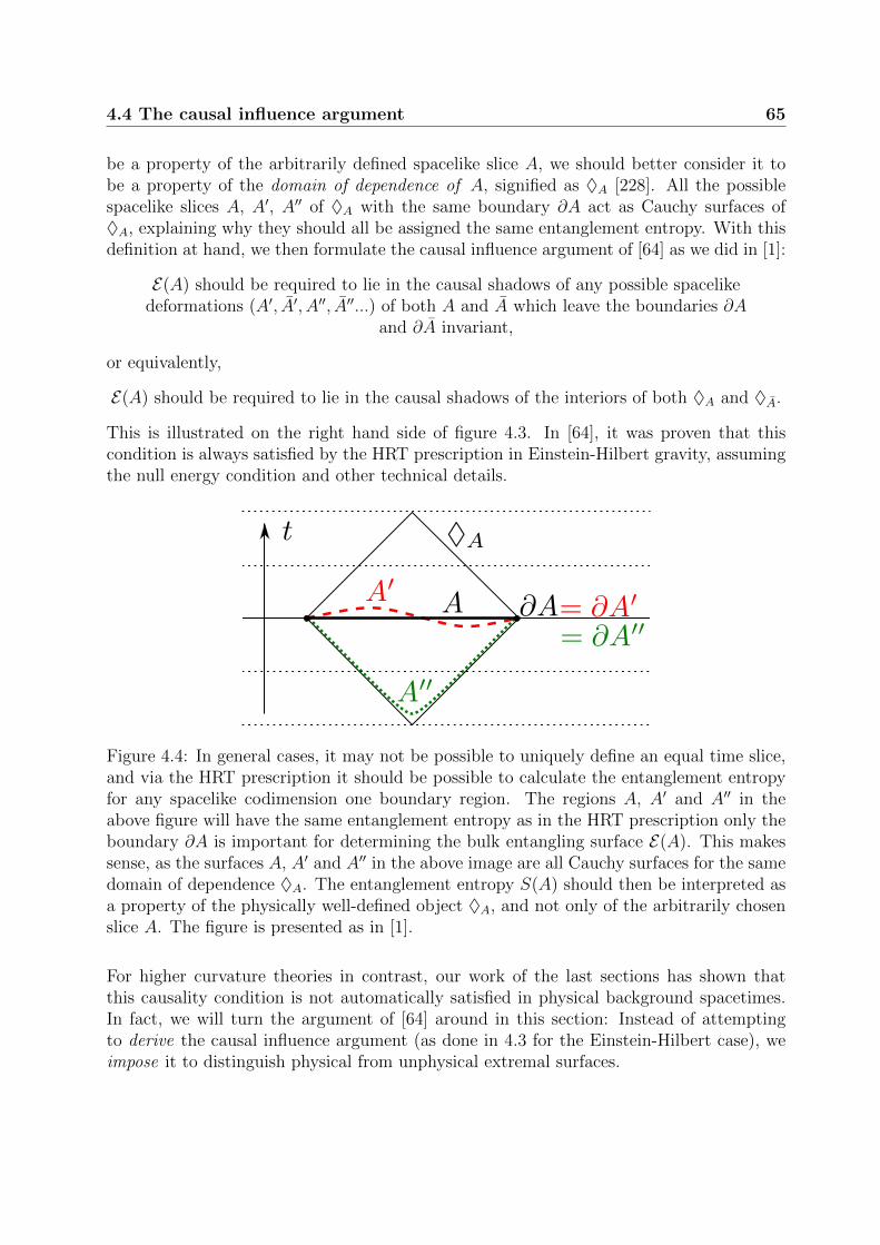
4.4 The causal influence argument 65

be a property of the arbitrarily defined spacelike slice A, we should better consider it tobe a property of the domain of dependence of A, signified as ♦A [228]. All the possiblespacelike slices A, A′, A′′ of ♦A with the same boundary ∂A act as Cauchy surfaces of♦A, explaining why they should all be assigned the same entanglement entropy. With thisdefinition at hand, we then formulate the causal influence argument of [64] as we did in [1]:

E(A) should be required to lie in the causal shadows of any possible spacelikedeformations (A′, A′, A′′, A′′...) of both A and A which leave the boundaries ∂A

and ∂A invariant,

or equivalently,

E(A) should be required to lie in the causal shadows of the interiors of both ♦A and ♦A.

This is illustrated on the right hand side of figure 4.3. In [64], it was proven that thiscondition is always satisfied by the HRT prescription in Einstein-Hilbert gravity, assumingthe null energy condition and other technical details.

Figure 4.4: In general cases, it may not be possible to uniquely define an equal time slice,and via the HRT prescription it should be possible to calculate the entanglement entropyfor any spacelike codimension one boundary region. The regions A, A′ and A′′ in theabove figure will have the same entanglement entropy as in the HRT prescription only theboundary ∂A is important for determining the bulk entangling surface E(A). This makessense, as the surfaces A, A′ and A′′ in the above image are all Cauchy surfaces for the samedomain of dependence ♦A. The entanglement entropy S(A) should then be interpreted asa property of the physically well-defined object ♦A, and not only of the arbitrarily chosenslice A. The figure is presented as in [1].

For higher curvature theories in contrast, our work of the last sections has shown thatthis causality condition is not automatically satisfied in physical background spacetimes.In fact, we will turn the argument of [64] around in this section: Instead of attemptingto derive the causal influence argument (as done in 4.3 for the Einstein-Hilbert case), weimpose it to distinguish physical from unphysical extremal surfaces.

66 4. Entanglement entropy in higher curvature theories

Figure 4.5: Application of the causal influence argument to a black hole spacetime. For aspacelike slice A that is an entire equal time slice of the right boundary, only the bifurcationsurface B satisfies the causal influence argument. The green dashed and red dotted linesshow possible configurations of additional extremal surfaces as the cases b) and d) in figure4.1. The figure is presented as in [1].

In the case of a static black hole spacetime, such as the BTZ black hole studied in section4.2, this argument is sketched in figure 4.5. The region A is assumed to be an entirespacelike slice of the right boundary, consequently the complement A is a slice of the leftboundary. The domains of dependence ♦A and ♦A are then the entireties of the right andthe left boundaries, respectively. The sets of points that can both receive signals fromand send signals to the interiors of ♦A or ♦A are called the causal wedges A and A,respectively [228, 229]. See also figure 4.3. By definition, these causal wedges A and Areach all the way from the boundary to the event horizon of the black hole. Additionally,all the points inside of the black hole event horizon are in one way causal contact with both♦A and ♦A, and are hence also excluded by the causal influence argument. This argumenthence rules out any possible closed extremal surface of the types b), c) and d) in figure 4.1.Only the bifurcation surface B is left over as a surface determining the physically correctentanglement between the two boundary CFTs. We hence recover the notion, explainedin section 3.3, that the black hole entropy, calculated from the geometry of the bifurcationsurface B according to Wald’s formula (4.2), should have the holographic interpretationof being the entanglement entropy between the two CFTs living on the two conformalboundaries of the eternal black hole spacetime.

In section 4.3, we also mentioned that technically closed extremal surfaces may also appearin spacetimes with only one asymptotic boundary, such as global AdS or boson star space-times. These surfaces satisfy the homology condition, and when attempting to determinethe entropy of the entire boundary CFT state via holographically calculating entanglemententropy, the only other option would be the empty surface, i.e. no surface at all. As thesespacetimes do not have event horizons, every point in the bulk is in causal contact withthe boundary, and consequently any possible closed extremal curve in the bulk would beruled out due to the causal influence argument. Consequently, the entanglement entropy is

4.4 The causal influence argument 67

trivially defined by the empty surface to be zero, which is the result physically demandedfor a pure state (see section 3.1).

We hence obtain the desired result, namely that the causal influence argument introducedabove is a reliable tool to, at least in the concrete examples studied in sections 4.2 and4.3, distinguish the physical surfaces extremising the entropy functional (4.4) from theunphysical additional extremal surfaces that we have found to occur. However, after thepublication of [1], doubt on the physical validity of Gauss-Bonnet gravity for any non-perturbative λ has been cast by [210]. Consequently, it may be necessary to turn thelogic of the above chapter around: Instead of using the causal influence argument todistinguish between physical and unphysical curves, one might hold the viewpoint thatthe existence of entangling curves violating the causal influence argument is a generalsign of an unphysical bulk theory. This viewpoint was indeed advocated for in [64], butinvestigations into this topic are still ongoing [201, 225, 226]. This closes our investigationof holographic entanglement entropy in bulk theories with higher curvature terms. In theremaining chapters 5 and 6 we will investigate the geometry and entanglement entropy oftoy models of holographic duals of boundary CFTs.

Chapter 5

Backreaction in holographic modelsof boundary CFTs

5.1 Holographic models of boundary CFTs

In the past sections we have studied models, both top-down and bottom-up, of dualitiesbetween gravitational theories on asymptotically AdS spacetimes and conformal field the-ories (CFTs) on the conformal boundary of these spacetimes, i.e. either on flat Minkowskispace or the (spacially compact) Einstein static universe. It is, however, also possible todefine CFTs on manifolds that have themselves a boundary, and these are called boundaryCFTs or in short BCFTs [230,231]. The study of BCFTs with codimension one boundariesis related to the study of CFTs with defects and interfaces as often such CFTs can be for-mulated as a BCFT [232]. By now, it should not come as a surprise to the reader that thereis a large variety of holographic models of such BCFTs or defect CFTs (see [233–236] fora partial list of references), and in the following we will especially focus on the bottom-upapproach introduced by Takayanagi et al. in [92–94].

The idea behind this type of model is sketched in figure 5.1. Here, N is an asymptoticallyAdS spacetime which, as before, we will call the bulk spacetime. The asymptotic conformalboundary of N is called M in figure 5.1, and this is where holographically the CFT isunderstood to live. So far, this is an ansatz just as in the regular AdS/CFT correspondence.Now, for a BCFT the manifold M on which this theory lives has to have a boundary foritself, namely P = ∂M . According to the bottom-up models of [92–94], this boundaryextends from M into the bulk spacetime N as a hypersurface Q, at which the spacetimeN abruptly ends. For reasons that will become fully clear in section 6, we refer to thishypersurface as the brane, but the reader should be aware that it is not any of the stringtheoretic branes used in 2.3 for example. Also, there is often confusion about the meaningof the words “boundary” and “bulk” in the context of BCFT. Pure field theory papers oftenuse “boundary” for P and “bulk” for M in figure 5.1, but in holography this nomenclature

70 5. Backreaction in holographic models of boundary CFTs

is usually avoided because it would conflict with the standard AdS/CFT convention to callM the boundary and N the bulk. We will hence refer to P as the defect. When discussingthe embedding of Q into N , will also refer to the latter as the ambient spacetime.

t

xz

Figure 5.1: Geometric setup for a bottom-up AdS/BCFT model according to [92–94]. The(asymptotically) AdS bulk spacetime N has the usual conformal boundary M as well asthe timelike hypersurface Q on which the spacetime ends. The intersection of Q and Mis referred to as P . The coordinates t, x, z follow the usual conventions for the Poincarepatch (2.11). The figure is presented as in [2].

The proposal of [92–94] suggests that the action for the bulk metric gµν should be amendedwith the usual Gibbons-Hawking boundary term [237] and counter term Σ(h) [126,146] onM (where h is the induced metric on M), but also with boundary terms on Q (inducedmetric γ) and P :

S =1

2κ2N

∫N

dd+1x√−g (R− 2Λ) +

1

κ2N

∫M

ddx√−h(K(h) − Σ(h)

)(5.1)

− 1

κ2N

∫Q

ddx√−γK(γ) +

∫Q

ddx√−γ LQ + SP .

In this formula, the quantities K(h) and K(γ) are the traces (with respect to the inducedmetrics hij and γij) of the extrinsic curvature tensors of M and Q, respectively. The signof K has to be fixed by a convention on where the normal vector to the surface in questionpoints, for M we conventionally assume that the normal vector is oriented to the outsideof the spacetime, while on the brane Q we choose the normal vector to be pointing intothe bulk. This will be the more convenient convention later is chapter 6. See appendixA.2 for definitions and further explanations. In (5.1), we have omitted terms for possiblematter fields living in N .

The model (5.1) explicitly includes the term ∼ LQ which describes matter fields livingon the worldvolume of the brane Q. These matter fields together with the embeddingof the brane Q into the ambient spacetime N will in these models (5.1) then constitutethe holographic description of the defect P and the BCFT degrees of freedom potentially

5.2 Energy conditions and their impact on the bulk geometry 71

restricted to it. Imposing Neumann boundary conditions on the bulk metric gµν at Q, weobtain the equations of motion [92–94]

Kij − γijK = −κ2N Sij, (5.2)

where γij is the induced metric on Q and Sij is the energy-momentum tensor derived fromthe matter Lagrangian LQ. The letter S was chosen to mean “surface” or “shell”. Thisway, we also distinguish the energy-momentum tensor on Q, Sij, from the bulk energy-momentum tensor, conventionally denoted Tµν . Equation (5.2), together with the equationsof motion for the matter fields described by LQ, has to be combined with the equationsof motion of bulk fields, such as for example the bulk metric gµν , for a full description ofthe classical bulk theory that is holographically dual to the BCFT defined on M and P .For the moment this prescription may seem rather abstract, but we will see a concrete andwell motivated realisation of this setup in chapter 6, other work on setups of the type (5.1)was presented in [238–245]. In the remainder of this chapter, we will collect a number ofresults on general setups of this type that were discussed in [2].

5.2 Energy conditions and their impact on the bulk

geometry

5.2.1 Decomposition of the energy-momentum tensor

In this section, we will in detail study the equations of motion (5.2). Specifically, we willconsider the case of a 2 + 1-dimensional bulk spacetime, such that both the AdS boundaryand the brane Q are 1 + 1 dimensional, as this is the relevant case for the holographicKondo model to be discussed in section 6.2.

As we will see now, in this case the equations (5.2) can be considerably simplified andmade tractable. The reason for this is that when Q is a 1 + 1-dimensional timelike brane,its worldsheet lightcone degenerates into two distinct null directions. We make use of thisby defining the worldvolume null vectors

lili = 0 = rir

i, liri = −1, (5.3)

where l stands for left pointing and r stands for right pointing. Note that this definitiondoes not completely fix the two vectors li, ri for a given induced metric γij, as there is stilla residual boost symmetry: li → ali, ri → 1

ari. Many of the expressions that we derive in

the following will be invariant under such boosts, but later we will restrict our interest tostatic cases, where both the ambient spacetime N and the brane Q have a timelike Killingvector field ∂t. One can then fix the boost symmetry by demanding li + ri ∼ δit.

The use of defining this null vector basis is that we can now decompose the energy-

72 5. Backreaction in holographic models of boundary CFTs

momentum tensor into scalar quantities by writing

Sij =S

2γij + SLlilj + SRrirj with (5.4)

S = γijSij, SL = rirjSij, SR = liljSij. (5.5)

Obviously, S is the trace of Sij while SL and SR parametrise the non-trace part of theenergy-momentum tensor. These three scalars then define the symmetric (0, 2) tensor Sij.

5.2.2 Energy conditions

In a next step we can now formulate energy conditions for Sij using the decomposition(5.4)1. Often in general relativity, it is of interest to derive certain results concerningsolutions of Einstein’s equations even when the specific form of the energy-momentumtensor is not known. In these cases, one usually uses energy conditions, i.e. conditionsimposed on the energy-momentum tensor that seem physically reasonable, for example thecondition that no observer should ever measure a negative energy density. It should bepointed out that there are many different energy conditions, some stricter than others, andnot all of them are satisfied even by physical matter models as we will see. For a reviewon this fascinating topic, see [246,247]. We will use:

• The null energy condition (NEC): For every null vector mi in the worldvolume of thebrane we have

Sijmimj ≥ 0 ∀ mimi = 0. (5.6)

The interpretation of the NEC is that a hypothetical null-observer will never measurea negative local energy density [247]. Using (5.4) it is easy to show that this implies

Sijlilj ≥ 0 and Sijr

irj ≥ 0 ⇒ SL ≥ 0 and SR ≥ 0. (5.7)

• The weak energy condition (WEC) generalises the NEC to timelike vectors:

Sijmimj ≥ 0 ∀ mimi < 0. (5.8)

The interpretation of the WEC is that no physical observer will ever measure anegative local energy density [247]. By continuity, the WEC implies the NEC. Pa-rameterising mi = αli + βri with α · β > 0 (this ensures that mi is timelike by (5.3))we then find

SL ≥ 0, SR ≥ 0, Sαβ ≤ SLα2 + SRβ

2 ∀α · β > 0. (5.9)

1Note that we will only formulate conditions on Sij in terms of the intrinsic geometry, i.e. the inducedmetric γij and vector fields living in the worldvolume of Q.

5.2 Energy conditions and their impact on the bulk geometry 73

Optimising the choice of α, β yields

SL ≥ 0, SR ≥ 0, S ≤ 2√SLSR. (5.10)

Note that these expressions are all invariant under the boosts of the null vectorsmentioned above.

• The strong energy condition (SEC) is well known in the literature of 3+1-dimensionalgeneral relativity, but the generalisation to arbitrary dimensions is not straightfor-ward. In our context, we will hence refer to the inequality

(Sij − Sγij)mimj ≥ 0 ∀ mimi < 0. (5.11)

as the SEC. This will prove to be very useful as the expression on the left hand sideappears when solving (5.2) for the extrinsic curvature:

Kij = −κ2N(Sij − Sγij) (5.12)

We have however no reason to believe that a physical matter field has to satisfy thisenergy condition, and in fact we will see later that in the holographic Kondo modelof section 6.2 it is indeed important that the matter fields violate this condition. Interms of scalar quantities, (optimising again the choice of α and β in mi = αli +βri)this yields

SL ≥ 0, SR ≥ 0, S ≥ −2√SLSR. (5.13)

We see that the SEC, just as the WEC, implies the NEC. On the other hand, WEC andSEC are unrelated. Not very surprisingly, the NEC is considered the most importantand reliable energy condition. Indeed, in this thesis we have already encountered somegeometric results that were proved using the NEC as a technical assumption in sections 3and 4. Although there are classical matter models that do even violate the NEC [246,247],it can be proven to be satisfied in string theory [248].

5.2.3 A corollary to the barrier theorem

The ultimate reason why we are interested in understanding the geometrical properties ofAdS/BCFT models is that eventually we would like to compute entanglement entropy inthe holographic Kondo model, as we will do in chapter 6. As we have seen in chapter 3,entanglement entropy of the boundary CFT is holographically encoded in the geometryof extremal (codimension 2) surfaces in the bulk spacetime. In a 2 + 1 dimensional bulk,entanglement entropy is hence defined by spacelike geodesics as we have already seen insection 3.2. In a setup such as the one shown in figure 5.1, it is obviously of interestwhether spacelike geodesics anchored at the boundary will, when they go deeper into thebulk, encounter the brane Q or whether they will stay in the interior of N . An intersection

74 5. Backreaction in holographic models of boundary CFTs

between the geodesics and the brane would potentially lead to a strong signature in thepattern of entanglement entropy measured at the boundary, explicit examples of this werediscussed in [2].

In order to investigate this issue in more detail, we can make use of the work of Engelhardtand Wall [249]. In this paper, the authors define the term extremal surface barrier to be acodimension one hypersurface that is embedded in an asymptotically AdS bulk spacetime insuch a way that extremal spacelike surfaces that are anchored on the AdS boundary to oneside of the extremal surface barrier cannot cross it. In the course of this thesis we will seeseveral explicit examples of surfaces that are extremal surface barriers, but in this sectionwe will be interested in the general statement of the theorem, and the implications that ithas on our models defined by (5.2). We state the result of [249] in our own nomenclature asintroduced in figure 5.1, section 5.1 and appendix A.2. There are some subtleties related towhether an extremal surface may touch the extremal surface barrier or not, which will notconcern us very much in the following. The theorem presented here as in [2] is a combinedresult of theorems 2.1, 2.2 and corollary 2.4 in [249].

Barrier Theorem (Engelhardt, Wall [249])Let Q be a codimension one hypersurface embedded in the spacetime N , which is assumedto end on Q and the AdS boundary M . If

Kijvivj ≤ 0 for any vector field vi on Q, (5.14)

then any Q-deformable spacelike extremal surface Υ which is anchored on the AdS bound-ary M remains in N , i.e. does not cross Q. By Q-deformable we mean that there is afamily Υa of extremal spacelike surfaces such that all of those are anchored on M , andcan be continuously deformed from some Υ0 ∈ Υa which is only located in N and doesnot touch Q.

Consequently, in the setup of figure 5.1, the geodesic defining the entanglement entropy fora boundary interval (which does not intersect with P ) on M cannot cross Q if the extrinsiccurvature on Q satisfies the assumption (5.14). See figure 5.2 for an illustration.

In [249] the authors were concerned with the geometric properties of general codimensionone hypersurfaces, but we are working with models in which the embedding of a brane Qinto an ambient spacetime is dynamically determined via the equation of motion (5.2). Wewill hence reformulate the assumption (5.14) made in the barrier theorem in terms of theenergy-momentum tensor Sij and express it in terms of energy conditions. This will becomplicated by the fact that (5.14) is supposed to hold for any (including spacelike) vectorfield vi while energy conditions are usually only phrased in terms of causal vector fields.

Using (5.12) and (5.4), we find that (5.14) can be written as

−S2viv

i + SL(livi)2 + SR(riv

i)2 ≥ 0. (5.15)

The last two terms are nonnegative due to the NEC, only the first term is potentiallyproblematic. We can now separately discuss this for the three different cases:

5.2 Energy conditions and their impact on the bulk geometry 75

Q2

Q3

Q4

Υ0 Υ1

Υ2Υ3

M x

z

zQ1

Υ0Υ1

Υ2

Υ3

xM

Figure 5.2: Compared to figure 5.1, we suppress the time direction t and assume a staticembedding of the branes Qi into a static background N . Left: Q can be an extremalsurface barrier which bends back to the boundary in a ∪-shaped manner. No Q1 deformableextremal surface can reach deeper into the bulk than Υ2, and hence none of them can crossQ1 if it is an extremal surface barrier. Note that the dotted geodesic Υ3 would cross Q1, butit is not anchored on M with both endpoints, hence the barrier theorem does not applyto it. Right: Three possible cases for which the brane Qi is anchored to the boundaryonly once. We see that as we move the right anchoring point of the geodesics Υ on theboundary more and more to the right, they reach deeper and deeper into the bulk. Q4

is not an extremal surface barrier as it is crossed by Υ3, but Q3 is an extremal surfacebarrier. In fact, it satisfies the assumption (5.14) trivially as KQ3

ij = 0. Q2 is automaticallyan extremal surface barrier as it is completely behind the barrier Q3, even if it does notsatisfy (5.14). The figure is presented as in [2].

• S = 0: As said above, the NEC is enough to ensure (5.15) to be satisfied for any vi.

• S < 0: For null and spacelike vi, the NEC is again enough to ensure the validity of(5.15). For timelike vectors vi, (5.15) is equivalent to the SEC as defined in section5.2.2.

• S > 0: This is the least straightforward case, as here (5.15) is satisfied by null andtimelike vi (assuming NEC), but spacelike vectors need more investigation. Writingvi = −αli + βri (with α · β > 0) this takes the form

−Sαβ + SLβ2 + SRα

2 ≥ 0 for any α · β > 0, (5.16)

which can be identified as the WEC introduced in section 5.2.2, see (5.9).

To summarise, we have shown that the condition of (5.14) is, using the equations of motion(5.2), equivalent to demand WEC and SEC (both implying the NEC) to hold at the sametime. This means that the energy conditions satisfied or violated by the matter fields

76 5. Backreaction in holographic models of boundary CFTs

defined to live in the worldvolume of Q will have profound implications on the possibleembeddings of the brane Q into the ambient spacetime N . We will see this on specificexamples in section 5.3.2 and chapter 6. In appendix B we will comment on the possibleextension of the findings of this section to higher dimensions.

5.2.4 AdS and BTZ backgrounds

After having studied the equations of motion (5.2) in great generality, we will now specialisemore to the specific cases that we will be interested in for the remainder of this thesis.Specifically, we will be interested in background spacetimes N with a static line elementof the form

ds2 = gµνdxµdxν =

1

z2

(−h(z)dt2 +

dz2

h(z)+ dx2

), (5.17)

which is 2 + 1-dimensional Poincare AdS for h(z) = 1 and the BTZ black hole [130, 131]in Poincare coordinates for h(z) = 1 − z2/z2

H . For simplicity, we have set the AdS radiusL = 1. We will also be interested in static embeddings of the brane Q into this backgroundspacetime, defined by a function x(z) as for the examples in figure 5.2. On the worldsheetof the brane, we will then use the same coordinates t and z as in the bulk. The extrinsiccurvature then reads:

Ktt =1

N

(∂zx

h

2

(h′ − 2h

z

)),

Ktz = 0,

Kzz =1

N

(−∂ 2

z x+ ∂zx

(h

z(∂zx)2 +

1

z− h′

2h

)),

(5.18)

where N comes from the normalisation of the normal vector nµ, see also appendix A.2 formore information. For the induced metric we find

γij =

(gtt 0

0 gzz + (∂zx)2 gxx

)≡(−a(z) 0

0 b(z)

). (5.19)

where we have defined the positive functions a(z) and b(z). One can now easily write downthe null vectors ri and li (fixing their boost invariance by demanding r1 + l1 = 0) to find

Sij =S

2γij + SLlilj + SRrirj (5.20)

=S

2

(−a 00 b

)+SL2

(a −

√ab

−√ab b

)+SR2

(a√ab√

ab b

). (5.21)

From (5.18) and (5.19) we see that, due to the equation of motion (5.2), also Sij will haveto be diagonal in the coordinate system of our choice, implying SL = SR ≡ SL/R. This

5.2 Energy conditions and their impact on the bulk geometry 77

makes sense, as it means that an observer at rest on the worldvolume of our brane at fixedz-coordinate should not see a net flux of energy from the left to the right, or vice versa.This should be a prerequisite for a static geometry. We hence find

Sij =S

2

(−a 00 b

)+ SL/R

(a 00 b

). (5.22)

For later use, we will also define the traceless symmetric tensor appearing in this equationto be

γij ≡(a 00 b

), γij =

(1a

00 1

b

), γij γ

ij = 2 (5.23)

which can also be written as γij = γij + 2uiuj with the normalised timelike vector ui =(√a

0

)which satisfies

∇iui = 0, (5.24)

ui∇iuj =

(0

12γttγzz∂zγtt

). (5.25)

Just as the energy-momentum tensor Sij can in the static case be expressed in terms oftwo scalars S and SL/R in (5.22), the same decomposition can be applied to the extrinsiccurvature. For this, we define (5.2) as

Kij =K2γij +KL/Rγij, (5.26)

≡ − (Kij − γijK) = κ2N Sij. (5.27)

The equation of motion (5.2) then reads in scalar form

K = κ2NS and KL/R = κ2

NSL/R. (5.28)

While S and SL/R can be constrained by energy conditions as in section 5.2.2, the scalarsK and KL/R are dependent on the embedding profile x(z). The impact of the differentenergy conditions on the embedding are summarised in table 5.1.

A further important result can be derived by demanding conservation of the energy-momentum tensor using (5.22) and (5.23):

0 = ∇iSij =

1

2∂iSγ

ij + ∂iSL/Rγij + SL/R

(2uj∇iu

i + 2ui∇iuj). (5.29)

The term uj∇iui vanishes immediately due to (5.24). There are now two cases for the

index j:

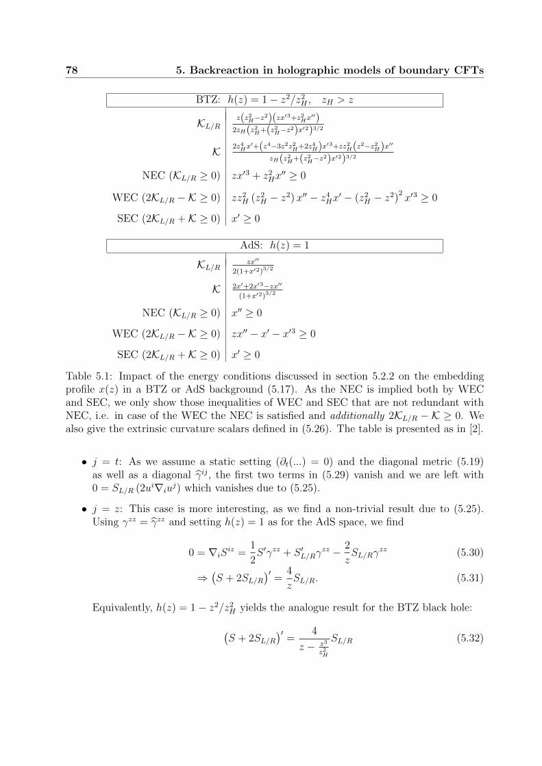
78 5. Backreaction in holographic models of boundary CFTs

BTZ: h(z) = 1− z2/z2H , zH > z

KL/Rz(z2

H−z2)(zx′3+z2

Hx′′)

2zH(z2H+(z2

H−z2)x′2)3/2

K 2z4Hx′+(z4−3z2z2

H+2z4H)x′3+zz2

H(z2−z2H)x′′

zH(z2H+(z2

H−z2)x′2)3/2

NEC (KL/R ≥ 0) zx′3 + z2Hx′′ ≥ 0

WEC (2KL/R −K ≥ 0) zz2H (z2

H − z2)x′′ − z4Hx′ − (z2

H − z2)2x′3 ≥ 0

SEC (2KL/R +K ≥ 0) x′ ≥ 0

AdS: h(z) = 1

KL/R zx′′

2(1+x′2)3/2

K 2x′+2x′3−zx′′(1+x′2)3/2

NEC (KL/R ≥ 0) x′′ ≥ 0

WEC (2KL/R −K ≥ 0) zx′′ − x′ − x′3 ≥ 0

SEC (2KL/R +K ≥ 0) x′ ≥ 0

Table 5.1: Impact of the energy conditions discussed in section 5.2.2 on the embeddingprofile x(z) in a BTZ or AdS background (5.17). As the NEC is implied both by WECand SEC, we only show those inequalities of WEC and SEC that are not redundant withNEC, i.e. in case of the WEC the NEC is satisfied and additionally 2KL/R − K ≥ 0. Wealso give the extrinsic curvature scalars defined in (5.26). The table is presented as in [2].

• j = t: As we assume a static setting (∂t(...) = 0) and the diagonal metric (5.19)as well as a diagonal γij, the first two terms in (5.29) vanish and we are left with0 = SL/R (2ui∇iu

j) which vanishes due to (5.25).

• j = z: This case is more interesting, as we find a non-trivial result due to (5.25).Using γzz = γzz and setting h(z) = 1 as for the AdS space, we find

0 = ∇iSiz =

1

2S ′γzz + S ′L/Rγ

zz − 2

zSL/Rγ

zz (5.30)

⇒(S + 2SL/R

)′=

4

zSL/R. (5.31)

Equivalently, h(z) = 1− z2/z2H yields the analogue result for the BTZ black hole:

(S + 2SL/R

)′=

4

z − z3

z2H

SL/R (5.32)

5.2 Energy conditions and their impact on the bulk geometry 79

These two equations are important for us because they have an interesting and straight-forward interpretation: By NEC, the right hand side of both (5.31) and (5.32) should bepositive, while the combination appearing in brackets on the left hand side is related to theSEC, see table 5.1 and section 5.2.2. Hence, the conservation of energy-momentum impliesthat if the NEC holds everywhere on the worldvolume of the brane and the SEC holds nearthe boundary, then the SEC will also hold deeper in the bulk, i.e. for larger z. This is alsoobvious from table 5.1: If x′′ > 0 everywhere and x′ > 0 near the boundary, then x′ > 0everywhere. The conservation of the energy-momentum tensor gives the deeper physicalreason for this.

Let us apply the findings of table 5.1 to the example embedding curves x(z) shown in figure5.2, assuming for simplicity that the background spacetime there is the Poincare AdS space.On the left hand side, we see that the embedding of Q1 starts with positive x′(z) and x′′(z),i.e. the SEC is satisfied by the matter fields on the brane. In our calculations so far andthe results presented in 5.1 we were, by the choice of the direction of the normal vector nµ,always implicitly assuming that if the brane is given by the embedding profile x(z), thenthe bulk spacetime N is located to the right of it, i.e. in the region x ≥ x(z). Consequently,our calculations and results of table 5.1 can only be applied to Q1 in figure 5.2 from thepoint x = 0, z = 0 up to the turning point of maximal z. In section 5.3.2 we will see explicitexamples of solutions of this form. On the right hand side of figure 5.2 we see that all ofthe depicted example embeddings satisfy the NEC, while Q2 clearly violates the SEC.

As an example of how the barrier theorem can be used in our context, let us propose thefollowing question: Suppose we want to solve the equations of motion (5.2) with an energy-momentum tensor that is defined by some kind of matter model where we can analyticallyprove that it has to satisfy, say, NEC and SEC. How might the solution for the embeddingqualitatively look like? Comparing to table 5.1, we immediately see that NEC and SECimply x′ ≥ 0 and x′′ ≥ 0. This rules out an embedding of the type Q2 shown in figure5.2, and if we assume a non-trivial energy-momentum tensor Sij 6= 0 this also rules outthe trivial totally geodesic embedding Q3. With NEC and SEC this is as far as we can go,but let us next also assume that in addition the WEC holds. Then the barrier theoremapplies, and the brane is an extremal surface barrier. If it would start on the boundary atx = z = 0 and go into the bulk indefinitely with x′ > 0, x′′ > 0, as Q4 in figure 5.2, thenwe could easily construct a spacelike geodesic anchored on M that intersects the branesomewhere in the bulk. All we would have to do is to move the one endpoint closer tothe brane, and the other one farther and farther away, until the geodesics reaches so deepinto the bulk spacetime that it intersects the brane. This would be in contradiction to thebarrier theorem, and hence a behaviour of the type of Q4 is also ruled out by SEC andWEC. The only possibility is a behaviour of the type of Q1: The brane has to bend backto the boundary. This means that WEC and SEC together force the brane to bend in a∪-shaped way. Conversely, if we want our brane to go deeper into the bulk without comingback to the boundary, either WEC or SEC has to be violated.

Suppose now that instead of a Poincare background we are working with a BTZ back-

80 5. Backreaction in holographic models of boundary CFTs

ground. A brane going from the boundary into the bulk, if it does not turn around andcome back to the boundary, will then encounter the event horizon. To study this in moredetail, let us take the entries of table 5.1 for the BTZ case and take the limit z → zH .Then we see that exactly at the horizon, WEC (x′(zH) ≤ 0) and SEC (x′(zH) ≥ 0) aremutually exclusive.2 We have seen that when both WEC and SEC are satisfied the branehas to turn around and bend back to the boundary, and our discussion has just shownthe converse: The brane (in the non-trivial case) can only enter the event horizon if eitherWEC or SEC is violated.

5.3 Exact solutions

Although the model (5.1) explicitly allows for generic matter fields to be defined on Q,most of the literature [92–94, 238–245] focuses on simple constant tension models, to bestudied in subsection 5.3.1. Notable exceptions are [245] where a perfect fluid living on thehypersurface Q is defined, and [242] where the case of a non-linear sigma model as mattercontent on Q is qualitatively discussed, apart from this the literature on exact solutions of(5.1) with non-trivial LQ is surprisingly sparse. In this section we will apply our analyses ofthe previous section in order to find simple analytical solutions of the equations of motion(5.2).

5.3.1 Constant tension solutions

The simplest possible model that can be studied using the equations (5.2) is the one wherethe energy-momentum tensor is defined by a constant tension λ:

Sij = −λγij ⇒ S = −2λ, SL/R = 0. (5.33)

For branes embedded in a global AdS3 background this model has already been studiedin [250], and we extensively commented on it in [2]. In this thesis we will only need theconstant tension solutions in a Poincare or BTZ background (5.17) which were studiedin [92].

Let us begin with the case for a Poincare background. From (5.28), (5.33) and table (5.1)we then find

0 = K =zx′′

2 (1 + x′2)3/2, (5.34)

−2λκ2N = K =

2x′ + 2x′3 − zx′′

(1 + x′2)3/2. (5.35)

2We have been assuming the general case x′ 6= 0 and x′′ 6= 0. Of course x′(zH) = 0 would be a possiblesolution, but note that the NEC implies that x′(z) is monotonously increasing. Hence, if the NEC holdsand x′(zH) = 0, then x′(z) = 0 for any z which is the trivial case.

5.3 Exact solutions 81

This has the solution

x′(z) =−λκ2

N√1− λ2κ4

N

= const., (5.36)

i.e. the corresponding embedding is just a straight line in Poincare coordinates. We alsosee that no solutions to (5.2) for a brane anchored at the boundary and embedded in aPoincare background exist when |λ| ≥ κ−2

N .

We see that for (5.33) with λ 6= 0, SEC and WEC are mutually exclusive: SEC woulddemand negative tension λ < 0 while WEC would demand positive tension λ > 0. Thismeans that these solutions show a behaviour that was already anticipated in our discussionin section 5.2: λ = 0 would be the trivial case Q3 in figure 5.2. The SEC satisfying butWEC violating case where λ < 0 and consequently x′(z) > 0 would be qualitatively similarto the curve Q4

3 in this figure, as the curve would go to the right and be intersected byspacelike geodesics. The WEC satisfying and SEC violating case λ > 0, x′(z) < 0 wouldbe qualitatively similar to Q2, in that it does not satisfy the property (5.14) but still isan extremal surface barrier simply because it is entirely on the far side of the extremalsurface barrier Q3. The positive tension case is generally considered to be physical whilethe negative tension case is considered the unphysical one, for several reasons. Firstly, theWEC is considered to be better motivated as a condition on physical theories that what wetermed the SEC in section 5.2.2 [247]. In fact we will see below that there are very sensiblemodels of field theories living on the brane worldvolume that effectively lead to constanttension models with positive tension only. Secondly, as the brane can intersect geodesics inthe negative tension case, it is not known how entanglement entropy for certain boundaryregions would then have to be calculated holographically. A proposal was made in [2] whichwould however be in conflict with the causal influence argument discussed in section 4.4.This geometric situation may be similar to the case described in [251] in that there are noextremal codimension two surfaces in the bulk spacetime connecting two boundary pointsin certain cases.

This situation is qualitatively similar in a BTZ background spacetime (5.17) where h(z) =1− z2/z2

H . There one finds the solution [92]

x(z) = −zHarctanh

sinh(s(λ))√z2H

z2 + sinh(s(λ))2

, tanh(s(λ)) = λκ2N . (5.37)

Here we have chosen the boundary condition x(0) = 0. This can be done without lossof generality due to the translation invariance of (5.17) in the x-direction. As pointedout in [2, 92, 250], the solutions (5.36) and (5.37) can be geometrically constructed via ageodesic normal flow, see figure 5.3 for an illustration in the AdS case. This constructionproceeds as follows: First, one determines the trivial embedding that solves the equations

3Except of course for the fact that Q4 would then have to be a straight line.

82 5. Backreaction in holographic models of boundary CFTs

(5.2) for zero tension λ = 0. By definition, this embedding will define a totally geodesiccodimension one hypersurface in the bulk spacetime. Next one constructs the geodesicsthat go through this surface normally, and shifts every point of this surface along the flowof these geodesics by an affine distance s which is a function of λ. This way the embeddings(5.36) and (5.37) for λ 6= 0 can be constructed.

Figure 5.3: Geodesic normal flow construction of a constant tension brane embedding in aconstant curvature background, here Poincare AdS. Points on the trivial λ = 0 embeddingare shifted along normal geodesics (dotted lines) by an affine distance s(λ).

The constant tension solutions that we discussed in this section will be important for tworeasons. First of all, the geodesic normal flow construction explained above makes it easyto obtain analytical results for embeddings such as (5.36) and (5.37), but also for theentanglement entropy of certain intervals. This is because the spacelike geodesics that areexplicitly used in this construction define the entanglement entropy of certain boundaryintervals, and increasing the tension, say, from λ = 0 to λ = λ0 > 0, we see that all thesegeodesics get longer exactly by a distance s(λ). Hence, according to the Ryu-Takayanagiprescription explained in section 3.2, the entanglement entropy of all these intervals willgrow by the same amount s(λ)/4:

S(λ,∆x) = S(λ = 0,∆x) +s(λ)

4. (5.38)

We will make use of this in sections 6.4.2 and 6.5.

The second reason why constant tension solutions will be important for us is that they canbe mimicked by a gauge field as we will now see. If the two-dimensional action of the fieldsliving on the brane only contains a U(1) gauge field

S = −∫d2x√−γ 1

4fmnf

mn, (5.39)

with no sources, then the energy-momentum tensor reads

Sij = −1

4fmnfmnγij + γmnfmifnj (5.40)

⇒ S =1

2fmnfmn (5.41)

5.3 Exact solutions 83

and the traceless part of (5.40) reads

Sij −S

2γij = −1

2fmnfmnγij + γmnfmifnj. (5.42)

The equation of motion in the absence of sources,

∂m(√−γγmpγnqfpq

)= 0, (5.43)

can then be shown to yield√−γf 01 = C with a constant C. It should be noted that due to

the antisymmetry of fmn and the fact that we are working in two dimensions, f 01 is the onlyindependent component of the field strength tensor. Using this and assuming a static casewith metric (5.19), it is then possible to show fmnfmn = −2C2 and γmnfmifnj = −γijC2.Consequently the traceless part (5.43) vanishes and the energy-momentum tensor (5.40)takes the form

Sij = −1

2γijC2. (5.44)

We hence see that in the absence of charges, the U(1) gauge field mimics a constant tensionmodel with positive tension.

5.3.2 Perfect fluid models

Let us consider a toy model where the energy-momentum tensor Sij on the brane is givenby a perfect fluid4

Sij = (ρ+ p)uiuj + pγij, (5.45)

with ui ∼ (1, 0) for staticity, and an equation of state

p = a · ρ. (5.46)

The usual decomposition into scalar quantities then tells us

S = p− ρ = ρ(a− 1), SL/R =p+ ρ

2= ρ

1 + a

2. (5.47)

and consequently the energy conditions take the form (assuming ρ ≥ 0)

NEC: a ≥ −1, WEC: a ≥ −1, SEC: a ≥ 0. (5.48)

4The ansatz that we follow in this section is different from the one presented in [245] in that we areworking in one dimension less. Also, we will explicitly pick an equation of state, while in [245] the equationof state is fixed by the specific ansatz.

84 5. Backreaction in holographic models of boundary CFTs

Let us now first work in a Poincare background, i.e. (5.17) with h(z) = 1. A useful way tosolve this equation is to use (5.31) which now reads5

ρ(z)′ =1 + a

a

ρ(z)

z⇒ ρ(z) =

c

κ2N

z1+ 1a , (5.49)

where we introduced a constant c. Now (5.28) together with K from table 5.1 allows us tosolve

x′(z) =acz

12(2+ 2

a)√1− a2c2z2+ 2

a

, (5.50)

x(z) =a2cz2+ 1

a 2F1

(12, 1+2a

2+2a; 3+4a

2+2a; a2c2z2+ 2

a

)1 + 2a

, (5.51)

with the hypergeometric function 2F1(a, b; c; d). Studying these expressions we see that,demanding x(z) to be real, these curves only reach the boundary for a ≥ 0 (i.e. SEC) anda ≤ −1. As we demand the NEC to be satisfied and the branes to be anchored at theboundary, we will from now on focus on a ≥ 0, i.e. both WEC and SEC being satisfied.

The solution (5.51) is only real for 0 ≤ z ≤(

1a2c2

) a2a+2 , and the derivative x′(z) diverges

as this limit is approached. This indicates that the embedding curves x(z) turn aroundand go back to the boundary, which as we have seen in section 5.2 is demanded by thebarrier theorem in the case where SEC and WEC are satisfied. The solution (5.51) hencedescribes an embedding similar to Q1 in figure 5.2. See figure 5.4 for plots of these solutionsfor different values for a and c.

This calculation can easily be generalized in two ways. First of all, we can add a constanttension contribution Ω to the energy-momentum tensor:

S = −2Ω + ρ(a− 1), SL/R = ρ1 + a

2. (5.52)

Secondly, we can generalise the Poincare background used above to a BTZ background(5.17), h(z) = 1 − z2/z2

H . Again, we can solve the equation (5.32) implying conservationof the energy-momentum tensor and find

ρ(z) =c

κ2N

(z2z2

H

z2H − z2

)a+12a

(5.53)

5This is basically the equation of motion for the perfect fluid. We could also look at the equation ofparticle number conservation, which in the static case is trivially satisfied as

∇i(n(ρ(z))ui

)= ui∂in(ρ(z)) + n(ρ(z))∇iui = 0,

where we can use (5.24), uz = 0 and ∂tn(ρ(z)) = 0 to show that this equation is satisfied. The particlenumber density n is related to the energy density ρ by the equation of state, see [252] for more information.

5.3 Exact solutions 85

0

1

z

1 x0

1z

1 2 xM M

Figure 5.4: Left: Brane profiles (5.51) for c = 1/a and, in order of increasing secondintersection with the x-axis, a ≈ 0.1, 0.2, 0.4, 0.7, 1.1, 2.0, 4.8, 100. Right: Brane profileswith a = 1 and, from outer to inner curve, c = 0.5, 1, 1.5, ..., 5. All the turning points lieon the dashed straight line. For clarity we added arcs leading back to the boundary in asymmetric way on both sides of the figure. We chose κ2

N = 1 for both the left and the rightfigure. The figure is presented as in [2].

which generalises (5.49). Interestingly, this result does not depend on the constant Ω. Inthe next step towards solving the equations of motion (5.28) for the given matter content(5.52), we use the results of table 5.1 to write

2aρ(z)− 2Ω = S + 2SL/R = K + 2KL/R =2zHx

′+(z)√

(z2H − z2)x′+(z)2 + z2

H

, (5.54)

where for simplicity we set κ2N = 1 from now on. This combination of terms only includes

x′(z) but not x′′(z), hence it can be algebraically solved for x′(z) to give

x′(z) =F(z)zH√

F(z)2z2 − F(z)2z2H + 4z2

H

, F(z) ≡ 2aρ(z)− 2Ω. (5.55)

For the general case this can only be integrated numerically to give the embedding profilex′(z), see the left hand side of figure 5.5. Even without an analytical solution for x(z), theexpression (5.55) gives us some information on the geometry of the brane embeddings, aswe see that x′(z) diverges to infinity at

z∞ =

√F(z∞)2 − 4

F(z∞)zH . (5.56)

Solving this equation exactly is hard, but for z → zH , we see from (5.53) and (5.55) thatF diverges for a > 0, and hence (5.56) will always have a real solution z∞ ≤ zH . Hencewe expect that even in a BTZ background, and even in the presence of a cosmologicalconstant term the branes will always turn around and bend back to the boundary. This isindeed the behaviour seen in figure 5.5.

86 5. Backreaction in holographic models of boundary CFTs

z

0 1 x

1

1

z

1x

0 MM

Figure 5.5: Left: Embedding functions for the brane with a perfect fluid in a BTZ back-ground with zH = 1. Depicted are the cases for Ω = 0, a = c = 1 and, in order of increasingsecond intersection with the x-axis, zH = 0.5, 1, 1.5, ..., 3. Additional symmetric branchesleading back to the boundary after the turning point were added. Right: Embeddingfunctions (5.57). Shown are the cases for a = c = 1 and, in order of increasing secondintersection with the x-axis, Ω = 2, 1, 0,−1,−2. We chose κ2

N = 1 for both the left andthe right figure. The figure is presented as in [2].

Equation (5.55) simplifies on a Poincare background, where zH →∞. It can then actuallybe integrated analytically, and one finds for the embedding function

x(z) =z

(1 + 2a)2√

1− Ω2(5.57)

×

[Ω(2a− 2)F1

(a

1 + a;1

2,1

2;1 + 2a

1 + a;acz1+ 1

a

1 + Ω,acz1+ 1

a

Ω− 1

)

+ 2a2cz1+ 1aF1

(2 + a

1 + a;1

2,1

2;3 + 2a

1 + a;acz1+ 1

a

1 + Ω,acz1+ 1

a

Ω− 1

)]where F1(a; b, c; d; e, f) is the Appell hypergeometric function. See the right hand side offigure 5.5 for a plot of such curves.

We have no specific boundary theory in mind that we hope this simple perfect fluid modelstudied in this section to be dual to, even on a qualitative bottom-up level. Nevertheless,we think that the investigations of this section were a worthwhile digression from our maininterest (the holographic Kondo model) for two reasons: First of all, the exact solutionspresented in this chapter demonstrate how tractable our analysis has made the equationsof motion (5.2), and it nicely demonstrates the impact of the barrier theorem on thegeometry of the embedding. Secondly, as we are now going to show, this perfect fluid canbe reformulated as a massless free scalar when the equation of motion parameter is chosento be a = 1.

5.3 Exact solutions 87

Assume the action of the scalar field living on the brane worldvolume to be

Lmatter,Q = −1

2γij∂iφ∂jφ. (5.58)

The equations of motion that follow from this model are

γ′11φ′ − 2

zγ11φ′ + 2γ11φ′′ = 0 (5.59)

and can be identified with (5.49) for a = 1 by setting

ρ ≡ 1

2γij∂iφ∂jφ =

γzz

2(φ′)

2. (5.60)

Similarly, using this substitution and a = 1 the energy-momentum tensor derived from(5.58) takes the form (5.47).

This result is noteworthy because the scalar model (5.58) is a special case of the non-linearsigma models discussed in [242]. There, it was suggested that these models would have aholographic interpretation as describing a boundary RG flow. Unfortunately, we have seenthat due to the consequences of the barrier theorem the branes in this model will have tobend back to the boundary as in figure 5.4, a behaviour that seems hard to interpret interms of a holographic RG flow. In fact, from the results presented in this section thisbehaviour of bending back to the boundary seems quite generic as it happens both inPoincare and BTZ backgrounds and even if due to the presence on a constant tension termthe SEC is violated near the boundary. In chapter 6 on the other hand, we will study aspecific model which does have an interpretation as the dual of a physical and well-definedholographic RG flow. In this model we will also find that the brane does not bend back tothe boundary, which in itself should be considered a non-trivial feature after the experiencegathered from the examples studied above.

Chapter 6

Entanglement entropy in aholographic Kondo model

We will now proceed to the central interest of this thesis, namely the Kondo effect and theholographic Kondo model of [86]. As we want to focus on presenting the contributions ofthe author to the study of entanglement entropy in the holographic Kondo effect carriedout in [2–4], we will only give a very brief review of the field theory physics of the Kondoeffect in section 6.1.1 following the overview given in [86]. The top-down model of [86] willthen be recapitulated in section 6.1.2 before summarising the bottom-up model of [86] insection 6.2. Genuine new results will then be discussed in great detail in sections 6.4-6.7.

6.1 Field theory and top-down model

6.1.1 Field theory

As already outlined in the introduction, the Kondo effect is a consequence of the spin-spininteraction between conduction electrons and dilute magnetic impurities [65]. Using thenotation of [86] in the following, the Kondo Hamiltonian describing the interaction of theelectrons with one impurity can then be written as [65]

HK = −ψ†α1

2m∇2ψα +

1

2λ′Kδ(~x)~S ψ†β

~Tβαψα. (6.1)

In this formula, the first term is the standard kinetic term for the conduction electronswhich are created and annihilated by the operators ψ†α and ψα. The α, β indices are

spin indices, and in the standard case of spin-12

particles with SU(2) symmetry ~T is justthe vector of Pauli matrices. The second term then describes the interaction betweenthe electron spins and the spin ~S of the impurity localised at ~x = ~0. As we saw in

90 6. Entanglement entropy in a holographic Kondo model

the introduction, the Kondo effect can be observed not only in traditional dilute alloys,but also in quantum dot systems. A unified description of the impurities that cause theKondo effect in these diverse situations can be given in terms of the Anderson impuritymodel [253], reviewed in [66]. See also figure 6.1. In this model, one considers a localisedsite to which electrons can be bound. If one single electron is bound to this site, thecorresponding energy level εd is below the Fermi energy εF of the surrounding conductionelectrons. However, for two electrons bound to this site the Coulomb repulsion U betweenthe two electrons raises the energy level above the Fermi energy. The state in which onesingle electron with an unpaired spin is bound to the localised site is hence energeticallypreferred, and the spin of this electron will act as magnetic impurity with respect to thesurrounding conduction electrons.

Figure 6.1: Illustration of the Anderson impurity model [253]. Electrons from a conductionband with Fermi energy εF can become bound to a localised site. Due to the Coulombrepulsion U , the state with one localised unpaired electron spin is energetically preferred.

As pointed out in [65], the Kondo effect is caused by an anti-ferromagnetic coupling λ′K >0. As the temperature of this system is lowered, it undergoes a renormalisation group(RG) flow which in the anti-ferromagnetic case leads to a growth and divergence of therunning coupling at the dynamically generated Kondo temperature TK [70]. At lowertemperatures, the system flows to a state in which the impurity is effectively screened byconduction electrons forming the Kondo screening cloud [70,72], see also [66,67,73,74] formore information on this state.

In the following, in order to pave the way for a holographic description of the Kondo effectwe will have to both simplify and generalise the model of (6.1). First of all, before applyingthe methods of the AdS/CFT duality to the Kondo system, we need to know whether andwhen CFT techniques can be used in the first place. Luckily, this topic has been studiedextensively by Affleck and Ludwig in [254–258]. As shown in [254], by only consideringthe s-wave channel of electrons interacting with the impurity and linearising around theFermi momentum kF , the model (6.1) simplifies to

HK =v

2πψ†Li∂xψL +

v

2λKδ(x)~S ψ†L

~TψL, (6.2)

where we have still used the notation of [86]. Specifically, v = kF/m is the Fermi velocity

and λK =k2F

2π2vλ′K . The s-wave reduction leads to in- and out-going fermions moving on

the radial coordinate 0 ≤ r < +∞, but for (6.2) this is mapped to a system of chiral

6.1 Field theory and top-down model 91

left-moving fermions ψL on the real line −∞ < x < +∞.1

This model (6.2) can then be treated by the methods of CFT and especially Kac-Moodyalgebras [254–258]. For us, the most important aspect of this is that the Kondo effect in3 + 1 dimensions, described by (6.1), obtains (at the fixed points) an additional conformalsymmetry when reduced to the effectively 1 + 1 dimensional model (6.2).

Furthermore, as in [86] we generalise the spin group from SU(2) to SU(Ns) and allow fork different channels or flavours of conduction electrons interacting with the impurity. Asdiscussed in [86, 87], the symmetry group of (6.2) is then a SU(N)k × SU(k)N × U(1)Kac-Moody symmetry. Here, the U(1) part stands for the electromagnetic charge. Onecan also study different representations of the impurity spin under SU(Ns) [259]. Thebenefit of promoting the spin group to SU(Ns) is that this enables the use of large Ns

techniques [259, 260]. It is known that in the large Ns limit, the formation of the Kondocloud happens as a phase transition similar to the phase transitions observed in models ofsuperconductivity, as part of the symmetry of the system is spontaneously broken [261–264].In particular, the limit studied in [86] was the one where Ns → ∞ and λK → 0 suchthat NsλK is kept fixed. Assuming the impurity spin to be in a totally antisymmetricrepresentation of SU(Ns), it can be phrased as [265]

Sa = χ†βTaβαχα, (6.3)

where the auxiliary fermions χa trapped to the localised site are referred to as slave fermionsor Abrikosov pseudo-fermions, see also [259,264]. In (6.3), the T a (a = 1, ..., N2

s −1) are theSU(Ns) generators in the fundamental representation, under which the χ transform. Thesefermions introduce an additional U(1) symmetry and unphysical states [265], a problemthat can be dealt with by imposing the constraint [86,259]

χ†χ = Q. (6.4)

This also means that the Young tableau of the impurity’s representation is a single columnwith Q < Ns boxes [86, 259]. Now, using (6.3) and the identity

T aαβTaγδ =

1

2δαδδβγ −

1

2Ns

δαβδγδ (6.5)

for the SU(Ns) generators, we find as in [86] that the spin-spin coupling in (6.2) can besimplified to

λKδ(x)~S ψ†L~TψL =

1

2λKδ(x)

(OO† − Q

Ns

ψ†LψL

), (6.6)

where we defined the operator

O = ψ†Lχ. (6.7)

1In [90], where (6.2) was modelled by a spin-chain, the s-wave reduction has been commented on indetail.

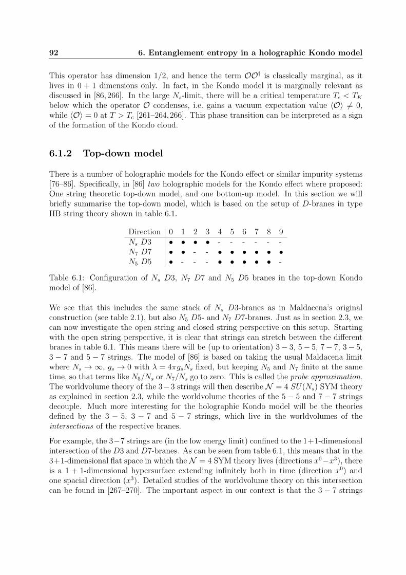
92 6. Entanglement entropy in a holographic Kondo model

This operator has dimension 1/2, and hence the term OO† is classically marginal, as itlives in 0 + 1 dimensions only. In fact, in the Kondo model it is marginally relevant asdiscussed in [86, 266]. In the large Ns-limit, there will be a critical temperature Tc < TKbelow which the operator O condenses, i.e. gains a vacuum expectation value 〈O〉 6= 0,while 〈O〉 = 0 at T > Tc [261–264,266]. This phase transition can be interpreted as a signof the formation of the Kondo cloud.

6.1.2 Top-down model

There is a number of holographic models for the Kondo effect or similar impurity systems[76–86]. Specifically, in [86] two holographic models for the Kondo effect where proposed:One string theoretic top-down model, and one bottom-up model. In this section we willbriefly summarise the top-down model, which is based on the setup of D-branes in typeIIB string theory shown in table 6.1.

Direction 0 1 2 3 4 5 6 7 8 9Ns D3 • • • • - - - - - -N7 D7 • • - - • • • • • •N5 D5 • - - - • • • • • -

Table 6.1: Configuration of Ns D3, N7 D7 and N5 D5 branes in the top-down Kondomodel of [86].

We see that this includes the same stack of Ns D3-branes as in Maldacena’s originalconstruction (see table 2.1), but also N5 D5- and N7 D7-branes. Just as in section 2.3, wecan now investigate the open string and closed string perspective on this setup. Startingwith the open string perspective, it is clear that strings can stretch between the differentbranes in table 6.1. This means there will be (up to orientation) 3− 3, 5− 5, 7− 7, 3− 5,3 − 7 and 5 − 7 strings. The model of [86] is based on taking the usual Maldacena limitwhere Ns →∞, gs → 0 with λ = 4πgsNs fixed, but keeping N5 and N7 finite at the sametime, so that terms like N5/Ns or N7/Ns go to zero. This is called the probe approximation.The worldvolume theory of the 3−3 strings will then describe N = 4 SU(Ns) SYM theoryas explained in section 2.3, while the worldvolume theories of the 5 − 5 and 7 − 7 stringsdecouple. Much more interesting for the holographic Kondo model will be the theoriesdefined by the 3 − 5, 3 − 7 and 5 − 7 strings, which live in the worldvolumes of theintersections of the respective branes.

For example, the 3−7 strings are (in the low energy limit) confined to the 1+1-dimensionalintersection of the D3 and D7-branes. As can be seen from table 6.1, this means that in the3+1-dimensional flat space in which the N = 4 SYM theory lives (directions x0−x3), thereis a 1 + 1-dimensional hypersurface extending infinitely both in time (direction x0) andone spacial direction (x3). Detailed studies of the worldvolume theory on this intersectioncan be found in [267–270]. The important aspect in our context is that the 3 − 7 strings

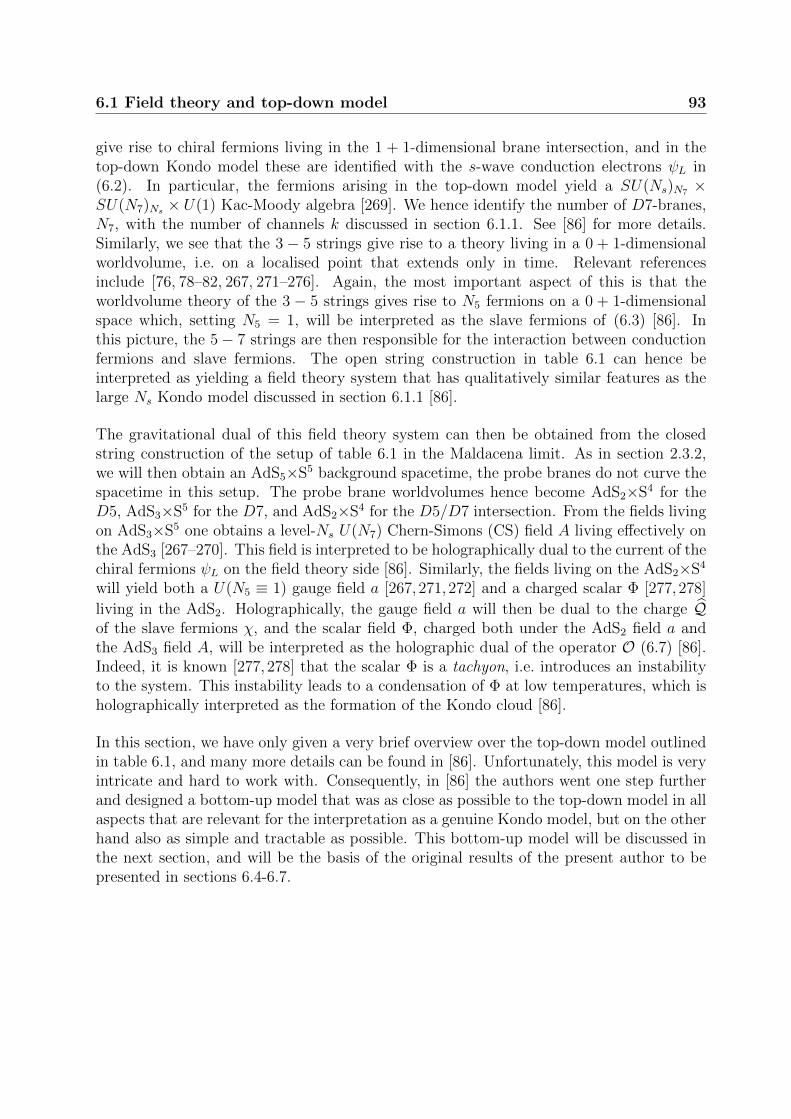
6.1 Field theory and top-down model 93

give rise to chiral fermions living in the 1 + 1-dimensional brane intersection, and in thetop-down Kondo model these are identified with the s-wave conduction electrons ψL in(6.2). In particular, the fermions arising in the top-down model yield a SU(Ns)N7 ×SU(N7)Ns × U(1) Kac-Moody algebra [269]. We hence identify the number of D7-branes,N7, with the number of channels k discussed in section 6.1.1. See [86] for more details.Similarly, we see that the 3 − 5 strings give rise to a theory living in a 0 + 1-dimensionalworldvolume, i.e. on a localised point that extends only in time. Relevant referencesinclude [76, 78–82, 267, 271–276]. Again, the most important aspect of this is that theworldvolume theory of the 3 − 5 strings gives rise to N5 fermions on a 0 + 1-dimensionalspace which, setting N5 = 1, will be interpreted as the slave fermions of (6.3) [86]. Inthis picture, the 5− 7 strings are then responsible for the interaction between conductionfermions and slave fermions. The open string construction in table 6.1 can hence beinterpreted as yielding a field theory system that has qualitatively similar features as thelarge Ns Kondo model discussed in section 6.1.1 [86].

The gravitational dual of this field theory system can then be obtained from the closedstring construction of the setup of table 6.1 in the Maldacena limit. As in section 2.3.2,we will then obtain an AdS5×S5 background spacetime, the probe branes do not curve thespacetime in this setup. The probe brane worldvolumes hence become AdS2×S4 for theD5, AdS3×S5 for the D7, and AdS2×S4 for the D5/D7 intersection. From the fields livingon AdS3×S5 one obtains a level-Ns U(N7) Chern-Simons (CS) field A living effectively onthe AdS3 [267–270]. This field is interpreted to be holographically dual to the current of thechiral fermions ψL on the field theory side [86]. Similarly, the fields living on the AdS2×S4

will yield both a U(N5 ≡ 1) gauge field a [267, 271, 272] and a charged scalar Φ [277, 278]

living in the AdS2. Holographically, the gauge field a will then be dual to the charge Qof the slave fermions χ, and the scalar field Φ, charged both under the AdS2 field a andthe AdS3 field A, will be interpreted as the holographic dual of the operator O (6.7) [86].Indeed, it is known [277, 278] that the scalar Φ is a tachyon, i.e. introduces an instabilityto the system. This instability leads to a condensation of Φ at low temperatures, which isholographically interpreted as the formation of the Kondo cloud [86].

In this section, we have only given a very brief overview over the top-down model outlinedin table 6.1, and many more details can be found in [86]. Unfortunately, this model is veryintricate and hard to work with. Consequently, in [86] the authors went one step furtherand designed a bottom-up model that was as close as possible to the top-down model in allaspects that are relevant for the interpretation as a genuine Kondo model, but on the otherhand also as simple and tractable as possible. This bottom-up model will be discussed inthe next section, and will be the basis of the original results of the present author to bepresented in sections 6.4-6.7.

94 6. Entanglement entropy in a holographic Kondo model

6.2 The bottom-up Kondo model

As said before, the bottom-up model of [86] is constructed in such a way as to be assimple as possible, while still providing a qualitative description of Kondo-like physics.Specifically, the holographic model will, by the limits discussed in sections 6.1.1 and 6.2 aswell as by the nature of gauge/gravity duality, provide a description of a magnetic impurity(with large spin) interacting with a strongly coupled system.

To this end, the bottom-up model discards many of the features and fields of the top-downmodel, while retaining the following ingredients [86]:

• A 2 + 1-dimensional asymptotically AdS bulk spacetime, such that the field theorymodel (6.2) can be interpreted as being the dual theory living on the AdS boundary.To describe the temperature dependence of the Kondo effect, the background space-time will be chosen to be a BTZ black hole (5.17). If the event horizon is located atz = zH in the coordinate system of (5.17), the temperature then reads [130,131]

T =1

2πzH. (6.8)

Furthermore, we assume the bulk theory action to contain an Einstein-Hilbert term

Sg =1

2κ2N

∫d3x√−g (R− 2Λ) , (6.9)

with the Ricci scalar R, the negative cosmological constant Λ = −1/L2 and the AdSradius L. In the following, we will set L = 1 for simplicity.

• A Chern-Simons (CS) field Aµ living in the 2 + 1-dimensional bulk spacetime, dualto the current of the chiral fermions ψL on the boundary. The action reads

SA = −N4π

∫Tr

(A ∧ dA+

2

3A ∧ A ∧ A

). (6.10)

The normalisation factor N is motivated from the action of the top-down modelof section 6.1.2, and is proportional to Ns. In the following, we will for simplicitychoose its gauge group to be U(1), correspondingly there will only be one channel ofconduction electrons, k = 1 [86].

• An asymptotically AdS2 subspace embedded in the background spacetime, with onetimelike direction and one radial direction. In the model of [86], this is simply takento be the slice of the BTZ spacetime defined by x ≡ 0. As this hypersurface is thebottom-up remnant of the D5/D7 intersection in the top-down model, we will referto it as the brane. The line element of the induced metric γij reads

ds2 = γijdxidxj =

1

z2

(−h(z)dt2 +

dz2

h(z)

), (6.11)

6.2 The bottom-up Kondo model 95

with h(z) = 1 − z2

z2H

. In the worldvolume of this brane, the model then includes the

action

Sa,Φ = −N∫d2x√−γ

(1

4fmnf

mn + γmn(DmΦ)†(DnΦ) + V (ΦΦ†)

), (6.12)

DmΦ ≡ ∂mΦ + iqAmΦ− iqamΦ , (6.13)

for a 1 + 1-dimensional gauge field am and a charged scalar Φ = φeiψ. Similar to thenomenclature of chapter 5, we use Greek indices for quantities in the 2+1-dimensionalbulk or ambient spacetime (e.g. gµν or Aµ) and Latin indices for quantities in the1 + 1-dimensional hypersurface x ≡ 0 (e.g. am,DmΦ, or γmn). The gauge group ofthe field am (dual to the charge of the slave fermions χ) is chosen to be U(1), whichis adequate for the single impurity case [86]. See [87] for a study of the two-impuritycase based on the same bottom-up model. The scalar field is charged both under thefield am and the CS field Am with opposite charges2, and in (6.13) we have explicitlyintroduced the value of the charge q compared to [86]. These charges will becomerelevant in section 6.3.2. As in the top-down model explained in section 6.1.2, thisscalar field will be interpreted to be holographically dual to the operator O = ψ†Lχand the condensation of this scalar at low temperatures will be interpreted as theformation of the Kondo cloud.

This model was sketched in figure 1.1. See [86,87] for an extensive discussion of this model,its features, and how good it describes Kondo physics via the holographic duality. Beforewe discuss how backreaction of the matter fields onto the bulk geometry can be taken intoaccount in the bottom-up model in section 6.3, we will briefly summarise some of the resultsobtained in [86] for the case without backreaction that will be important later on. First ofall, for high temperatures the system is in the normal phase, where the scalar Φ vanisheseverywhere and only the gauge field am is non-zero on the brane. In the convenient gaugeaz = 0, the solution to the equations of motion then reads

at(z) =Qz

+ µ, (6.14)

where, holographically,Q ≡ Q/Ns fixes the charge of the slave fermions defined in (6.4) [86].When solving the equations of motion of the Kondo model, a fixed value of Q has to begiven as a Neumann boundary condition [86], see also [279, 280] for related discussionsof vector fields in low-dimensional bulk spacetimes. At low temperatures, the scalar fieldwill condense, i.e. there will be a thermodynamically preferred solution to the equations ofmotion with φ(z) 6= 0. In [86], the potential of the scalar appearing in (6.12) was chosento be only a mass term

V (ΦΦ†) = M2ΦΦ†, (6.15)

2See appendix C for a definition of the quantity Am.

96 6. Entanglement entropy in a holographic Kondo model

which is the simplest non-trivial possibility. This is one of the aspects where the bottom-up model deviates strongly from the top-down model, as there the potential is much morecomplicated and not even known up to all orders [86]. We will comment on this issuemore in section 6.7. To obtain the correct conformal dimension of the dual operatorO, ∆ = 1/2, the mass M2 in (6.15) is chosen such that the scalar field saturates theBreitenlohner-Freedman [197] bound in AdS2. This also causes an instability such that atlow temperatures the scalar field shows a tendency to condense, see [266] for a review ofthe instabilities arising in the 1 + 1-dimensional case under consideration here. However,the effectively 1 + 1-dimensional case is special in the sense that due to the coupling of thescalar to the gauge field and the asymptotic behaviour (6.14), the scalar’s effective masswill get a contribution by Q [266], leading to the requirement (for the charge q = 1) [86]

M2eff = M2 −Q2 = −1

4. (6.16)

This means that in the model under consideration, the mass M2 has to be fixed to aspecific value depending on the choice of the boundary condition Q in order for the dualoperator of φ to have the right dimension [86]. With the above value of M2, the asymptoticnear-boundary behaviour of φ(z) is then

φ(z) = α√z ln(Θz) + β

√z + ..., (6.17)

where we introduced a scale Θ for-dimensional reasons. In order to understand the physicalmeaning of α and β, we have to remind ourselves that in the discussion of the GKPWformula in section 2.3.3, we dealt with operators that are sourced in the dual CFT byterms ∼

∫ddxOϕ(0). In contrast, from (6.6) we can see that the leading contribution of

the Kondo coupling to the field theory action in the large Ns limit is the term ∼ OO†.This is effectively a double trace deformation [86,281–283]. Defining what we will call theKondo coupling [86]

κ ∝ −NsλK , (6.18)

the holographic prescription to deal with such double trace deformations then yields

α ≡ κβ. (6.19)

See also [87] for a detailed discussion of this identification in the Kondo model. Interest-ingly, one finds that this coupling runs with the energy scale Θ when this scale is changedin (6.17) [282]. In particular, shifting the energy scale as Θ0 → Θ1 and demanding thephysical field φ(z) to be unchanged in (6.17), we can read off [86]

κ1 =κ0

1 + κ0 ln(

Θ0

Θ1

) . (6.20)

6.3 Backreaction in the Kondo model 97

Specifically, in the following we will want to use the temperature T as the energy scaledescribing the RG flow of the Kondo model. To this end we introduce tilded coordinatesin which zH is set to one, i.e. [86]

z = z/zH , x = x/zH , t = t/zH . (6.21)

As a consequence of these rescalings, we also find [86] that φ = φ and at = at zH . Equation(6.14) then yields

at =Qz

+ µT , (6.22)

where we have defined µT ≡ µ zH = µ/2πT [3]. This means that while keeping zH fixedin numerical calculations, we can still effectively vary the temperature by varying thecoefficient µT in the near-boundary expansion of at, as only the ratio µT ∼ µ/T is physicallymeaningful [3, 86]. Similar to (6.17), we define

φ(z) = αT√z log(z) + βT

√z + . . . (6.23)

with κT ≡ αT/βT and find

κT =κ(Θ)

1 + κ(Θ) log(ΘzH). (6.24)

This diverges at the Kondo temperature

TK ≡Θ

2πe1/κ(Θ), (6.25)

which satisfies [3]T/TK = exp(−1/κT ). (6.26)

We hence see that this bottom up-model has the potential to describe the qualitativeKondo-like features expected from a magnetic impurity interacting with a strongly coupledelectron system in the large Ns limit, including the formation of a Kondo cloud (conden-sation of Φ) and the existence of a dynamically generated scale (TK) [86]. The results tobe presented in the following sections will all be derived from this specific model. Hence,although other models for holographic impurities exist [76–85], it will be the bottom-upmodel discussed above that will for brevity be referred to as the holographic Kondo modelin this thesis.

6.3 Backreaction in the Kondo model

One of the most interesting aspects about the Kondo effect is the Kondo cloud, and itsproperties such as size and shape for example. So naturally we should ask how we caninvestigate the Kondo cloud using the bottom-up model presented in the previous section.

98 6. Entanglement entropy in a holographic Kondo model

In the heuristic picture 1.1, we have depicted the Kondo cloud as a swarm of electronssurrounding the impurity with anti-aligned spins. Although this is only a naive qualitativepicture of the CFT state, it gives us an idea about how the Kondo cloud could manifestitself in terms of objects that can be studied holographically. Namely, in section 3.1 wealready saw the simple example of a state (3.8) where two spins are correlated such thatthey have non-zero entanglement entropy, and similarly we expect that the Kondo cloudshould leave an imprint on the pattern of entanglement entropy in the field theory. Wehave seen in section 3.2 that entanglement entropy is a quantity that can be studiedcomparably easily in holography, but from the prescription (3.11) it is also clear that wewill only obtain non-trivial results on the entanglement entropy in the holographic Kondomodel if we include backreaction of the matter fields onto the geometry. How to do thiswill be the topic of this section, and in the following section 6.4 we will then present anddiscuss the results that we obtain on the entanglement entropy.

6.3.1 The Israel junction conditions

Looking at the model presented in section 6.2, we first of all note that the only fields thatare defined throughout the bulk spacetime are the metric gµν and the Chern-Simons fieldAµ. The latter is topological, and hence does not backreact on gµν . The only remainingmatter fields are the scalar Φ and the gauge field am which are constrained to live inthe worldvolume of a codimension one hypersurface embedded into the bulk spacetime.Naively, they would hence lead to an infinitely thin distribution of mass and energy, orequivalently to an energy-momentum tensor in the three-dimensional Einstein’s equationsthat has a δ-peak like shape. The correct framework to deal with this problem is providedby the Israel junction conditions [284], which can be geometrically understood in thefollowing way: The codimension hypersurface on which the matter fields Φ, an are definedsplits the bulk spacetime into two parts, one to the left of it and one to the right of it,see figure 6.2. To make contact with the topics discussed in chapter 5 (see especiallyfigure 5.1), we will refer to the hypersurface as Q, to the bulk spacetime as N and to theasymptotic boundary as M . Q then splits N into the two parts N+ and N− (with metricsg±), and similarly M into M+ and M−. The embedding of Q into N± is then given byan embedding profile x±(t, z), using coordinates of the Poincare patch. As in chapter 5,we can choose the boundary condition x±(0, 0) = 0 without loss of generality, due to thetranslation invariance of (5.17) in the x-direction.

The Israel junction conditions describe how the two spacetimes N± are glued togetheralong the common hypersurface Q. First of all, the hypersurface Q has to be embeddedinto the spacetimes N± in such a way that metrics γ± on Q that can be induced from theambient space metrics g± have to be equal: γ+ = γ− ≡ γ.3 The equality of the two inducedmetrics means, amongst other things, that a point on Q given by certain coordinates ofN+ can be identified with a point on Q in terms of coordinates on N−. It is in this sense

3See [285] for an exploration of cases in which this condition is not assumed.

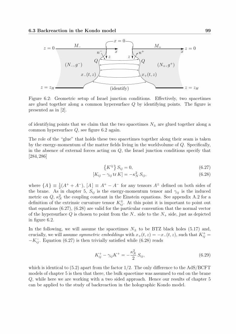
6.3 Backreaction in the Kondo model 99

x = 0

(identify)

(N−, g−)

M−

Q

xz = 0

z = zH

x−(t, z)

z = 0

z = zH

(N+, g+)

Q

M+

z zx

x+(t, z)

n+n−

Figure 6.2: Geometric setup of Israel junction conditions. Effectively, two spacetimesare glued together along a common hypersurface Q by identifying points. The figure ispresented as in [2].

of identifying points that we claim that the two spacetimes N± are glued together along acommon hypersurface Q, see figure 6.2 again.

The role of the “glue” that holds these two spacetimes together along their seam is takenby the energy-momentum of the matter fields living in the worldvolume of Q. Specifically,in the absence of external forces acting on Q, the Israel junction conditions specify that[284,286]

KijSij = 0, (6.27)

[Kij − γij trK] = −κ2N Sij, (6.28)

where A ≡ 12(A+ + A−), [A ] ≡ A+ − A− for any tensors A± defined on both sides of

the brane. As in chapter 5, Sij is the energy-momentum tensor and γij is the inducedmetric on Q, κ2

N the coupling constant in the Einstein equations. See appendix A.2 for adefinition of the extrinsic curvature tensor K±ij . At this point it is important to point outthat equations (6.27), (6.28) are valid for the particular convention that the normal vectorof the hypersurface Q is chosen to point from the N− side to the N+ side, just as depictedin figure 6.2.

In the following, we will assume the spacetimes N± to be BTZ black holes (5.17) and,crucially, we will assume symmetric embeddings with x+(t, z) = −x−(t, z), such that K+

ij =−K−ij . Equation (6.27) is then trivially satisfied while (6.28) reads

K+ij − γijK+ = −κ

2N

2Sij, (6.29)

which is identical to (5.2) apart from the factor 1/2. The only difference to the AdS/BCFTmodels of chapter 5 is then that there, the bulk spacetime was assumed to end on the braneQ, while here we are working with a two sided approach. Hence our results of chapter 5can be applied to the study of backreaction in the holographic Kondo model.

100 6. Entanglement entropy in a holographic Kondo model

There are indeed different ways how to derive the Israel junction conditions, and oneaction-formalism based method (see [287–289]) is to start with an action

S =1

2κ2N

∫N+

d3x√−g+(R+ − 2Λ+) + SN+ +

1

2κ2N

∫N−

d3x√−g−(R− − 2Λ−) + SN−

+1

κ2N

∫M+

d2x√−h+K

(h+) + SM+ +1

κ2N

∫M−

d2x√−h−K(h−) + SM− (6.30)

− 1

κ2N

∫Q

d2x√−γK(γ+) +

1

κ2N

∫Q

d2x√−γK(γ−) + SQ + SP

where we have terms similar to (5.1) both for the N+ side and the N− side, coupled toa common boundary Q. This corresponds to our view that the Israel junction conditionsdescribe the gluing of the two spacetimes N± = M± ∪ N± ∪ Q± ∪ P± along the commonhypersurface Q ≡ Q+ = Q− (intersecting the AdS boundary at P ≡ P+ = P−, P± =M± ∩ Q±). The above formula explicitly includes the possibility of matter terms in theambient spacetime (SN±), matter terms on the brane Q (SQ) as well as boundary andcounter terms on the AdS boundary (SM±) and on the intersection P , SP (see [288] andthe appendix in [94]). It should also be noted that we have fixed the signs of the extrinsiccurvature tensors K(γ±) according to our usual convention. It can then be shown that(6.30) yields the Israel junction conditions (6.28) [287–289].

x−(z) x+(z)

bulk bulk

hypersurface

boundary

identify points

boundary

Figure 6.3: Left: Geometric setup with independent coordinate systems on both sides ofthe brane, as in figure 6.2. Right: Gaussian normal coordinates in which the bulk metricgµν is continuous at the brane, but not differentiable. The figure is presented as in [3].

As a final comment on the Israel junction conditions, we should note that in the abovediscussion and derivation it is a priori possible to choose independent coordinate systemsin the bulk parts N±, as long as the induced coordinate system on Q is the same. Thisis why the brane has two distinct embedding functions x± with respect to the two bulkparts N± on both sides of it. As an alternative, it is in principle possible to constructGaussian-normal coordinates which cover a vicinity of the brane on both sides of it in a

6.3 Backreaction in the Kondo model 101

unified way. To do this, one starts by defining a coordinate system on Q and defines theaffine parameter of the geodesics normal to it as the additional coordinate in the higher-dimensional ambient space. This is similar to the construction employed in section 5.3.1.In Gaussian normal coordinates, it is easy to show that the bulk metric gµν is continuouson the brane, but not differentiable. In fact the discontinuity of the (normal) derivative ofthe metric on the brane Q is proportional to the expression K+

ij−K−ij . This discontinuity ofthe first derivative of the metric then leads to a δ-like peak in the curvature tensors at thelocation of the brane. In Einstein’s equations this δ-peak then balances the δ-peak in thebulk energy-momentum tensor Tµν that comes from the worldvolume energy-momentumtensor Sij exactly according to the equation (6.28). See [102] for an extensive discussion ofIsrael junction conditions in Gaussian normal coordinates. As explained in section 6.2, ourbulk spacetime does not only contain the metric gµν as a dynamical field, but also the CSfield Aµ. As this field also couples to the matter localised on the brane, it will enter ourcalculations with its own junction conditions. These are explained in appendix C, whereit is shown that the Chern-Simons field effectively decouples from the fields on the brane.

6.3.2 Equations of motion

The dynamical quantities in the bottom-up bulk model are the fields Φ, am, Aµ and, asdiscussed in the previous section, the embedding profile of the brane x+ ≡ −x−. The bulkmetric gµν is fixed to be a BTZ background (5.17), which is possible as the CS field doesnot backreact on the bulk geometry. Furthermore, the CS field Aµ effectively decouplesfrom the rest of the fields as discussed in appendix C. Choosing a static setup where noneof the dynamical variables depend on the t coordinate, and choosing a radial gauge az = 0(which also allows us to set ψ = 0, see [3]), the remaining dynamical quantities are thenφ(z), at(z) and x+(z). The equations of motion of this system then read

γijDiDjφ−M2φ = 0, (6.31)

∂z√−γf zt + J t = 0, (6.32)

Kij −κ2N

2Sij = 0 (6.33)

⇔ K =κ2N

2S and KL/R =

κ2N

2SL/R, (6.34)

where the current reads Jm = −2√−γγmnanφ2 and the extrinsic curvature quantities

Kij,K,KL/R have been defined in (5.26). The energy-momentum tensor following from theworldvolume action (6.12) reads [3]

S =N2fmnfmn − 2NV

(Φ†Φ

), SL/R =

N2γij(D(iΦ

)†Dj)Φ, (6.35)

102 6. Entanglement entropy in a holographic Kondo model

where γij was defined in (5.23). At the event horizon, or more accurately at the pointwhere the brane crosses the event horizon, the regularity conditions

φ′(zH) = −L2M2 φ(zH)

2zH, at(zH) = 0, x′+(zH) = κ2

NN2L4M2 φ(zH)2 − z 4

H a′t(zH)2

4L3

(6.36)have to be imposed [3]. As motivated above, for the study of entanglement entropy weneed solutions with non-trivial backreaction, an Kij that is not perturbatively small. From(6.33), we see that this requires κ2

NSij to be of order one in the large Ns limit that the top-down model requires. However, the gravitational coupling constant κ2

N = 8πGN is of order1/N2

s , and the factor N in (6.35) is of order Ns. We hence rescale all the fields to be oforder

√Ns, which for consistency is accompanied by a rescaling of the charges q in (6.13).

This is effectively the same as fixing κ2NN = 1 and q = 1, as was done for the numerical

calculations of [3]. However, it is important to note that in the next section we will see howthe physical properties (specifically energy conditions) of the fields of the bottom-up modelconstrain the qualitative solutions for the bulk geometry. Consequently, we believe thatthe solutions found numerically for the choice κ2

NN = 1 will be qualitatively representativefor the behaviour of the system at any value of κ2

NN . Furthermore, in section 6.5 we willderive a geometrical approximation formula that is only based on the most fundamentalgeometric properties of the bottom-up Kondo model, and hence does not depend on thespecific choices of the parameters made in the numerical calculations of [3].

Solving the equations of motion (6.31)-(6.33), one finds that there is a critical temperature

Tc ≈ 0.885TK (6.37)

below which there is a thermodynamically preferred solution with φ(z) 6= 0 ⇔ 〈O〉 6= 0,while above Tc the preferred solution is the normal phase in which φ(z) = 0⇔ 〈O〉 = 0 forany z [3]. This normal phase has an analytical solution due to the normal flow construction,as discussed in section 5.3.1. We then find [3]

at =CzH

cosh(s)

(cosh(s)−

√(zH/z)2 + sinh2(s)

)(6.38)

= −C cosh(s)

z+C cosh(s)2

zH. . . , (6.39)

x+(z) = −zH arctanh

sinh(s)√(zH/z)2 + sinh2(s)

, (6.40)

tanh (s) =1

4κ2NNC2 , (6.41)

where Sij = −N2γijC2 and C is the electric flux of the gauge field at the boundary. In the

numerical calculations of [3], which lead to the results presented below, we fixed C = 1/2in order to insure comparability with the results of [86], where the same choice was made.

6.4 Entanglement and defect entropy 103

By comparison with (6.14), we can also read off

Q = −C cosh(s) and µ =CzH

cosh2(s) (6.42)

from the above near-boundary behaviour. The solution (6.40) satisfies NEC and WECwhile violating SEC, as expected from the discussion in section 5.3.1.

It is important to note that for a non-trivial embedding, the line element of the inducedmetric will read (compare to (6.11))

ds2 =1

z2

(−h(z) dt2 +

1 + h(z)x′+(z)2

h(z)dz2

). (6.43)

Equation (6.40) shows that x′+(z) 9 0 as z → 0, and consequently the induced metric(6.43) may be asymptotically AdS2, but the effective AdS radius will depend on Q. Thisenters the Breitenlohner-Freedman bound of the scalar Φ, and instead of (6.16) we nowobtain [3]

M2 = Q2 − 1

4 cosh2 (s). (6.44)

This reproduces equation (6.16) in the limit of vanishing backreaction, where κ2NN → 0.

6.4 Entanglement and defect entropy

Details on how the equations of motion (6.31)-(6.34) can be solved numerically were givenin [3] and shall not be repeated here. Instead, we will start right away with the physicalinterpretation of these solutions in this section. In particular, we will discuss energy con-ditions and their impact on the geometry in (6.4.2). Section 6.4.2 will then be denoted toa discussion of our findings of entanglement and defect entropy in the Kondo model, whilein section 6.4.3 we will discuss the holographic g-theorem.

6.4.1 Energy conditions in the Kondo model

As we have discussed in section 6.3.2 (see also section 5.3.1), the normal phase is describedby a gauge field living on Q in the absence of charges, which is effectively a constanttension model (6.40) satisfying WEC and NEC, but violating the SEC. This violationof the SEC is a very important feature of the holographic Kondo model: We want todescribe one impurity on the boundary which is infinitely extended into the spacelikedirection x. This is why in the model without backreaction the brane goes straight fromthe boundary into the bulk and into the black hole event horizon as depicted in figure 1.1.

104 6. Entanglement entropy in a holographic Kondo model

If, however, the matter fields living on Q in the holographic model would satisfy both WECand SEC, we have seen in chapter 5 that this would force the brane to bend back to theboundary in a ∪-shaped way, as a consequence of the barrier theorem. This phenomenonof bending back to the boundary would also lead to an effective compactification of theboundary as the x-coordinate would now be restricted to a finite range of values, see [2]for a deeper discussion. Indeed, in section 5.3.2 we have seen several analytic solutionsof physical models where precisely this was the case. The fact that the matter fields inthe holographic Kondo model of section 6.2 violate the SEC everywhere in the bulk, andthe brane consequently shows the phenomenologically desired behaviour of going from theboundary into the event horizon (as a curve of type Q2 in figure 5.2), should hence beconsidered a non-trivial consistency check: The model derived and studied in [86] withoutbackreaction in mind still behaves physically reasonable when turning on backreaction.While it is possible to show analytically that the SEC is violated in the normal phase (seesection 5.3.1), for the condensed phase this is only possible numerically. We did indeedcheck that for all numerical solutions discussed in this section, both WEC and NEC aresatisfied while the SEC is violated everywhere.

The behaviour of the NEC is especially interesting as we numerically find that SL/R → 0in both the limits z → 0 and z → zH . The z → 0 is easy to understand: Near theAdS boundary, the scalar field goes to zero as (6.17)4 and the contribution of the gaugefield (6.39) becomes dominant. Hence we expect that near the boundary, our branes willasymptote to the exact solution for the normal phase (6.40) for any T/Tc. This expectationis indeed verified by our numerical solutions, see figure 6.4. The perhaps more surprisingcase is the one where z → zH . Using(6.35), (6.36), (5.23) and (6.43) one indeed finds

γ11 ∼ z2 − z2H = (z − zH)(z + zH), (6.45)

γ00 ∼ (z2 − z2H)−1 = (z − zH)−1(z + zH)−1, (6.46)

φ′ ∼ const. , (6.47)

φ ∼ const. , (6.48)

at ∼ z − zH , (6.49)

as z → zH and hence SL/R → 0 in this limit. This means that even for T/Tc 6= 1 ourbranes can be approximated by a constant tension brane both in the near-boundary andin the near horizon regime. This will be useful in section 6.5.

The numerically obtained embedding profiles for x+(z) for different temperatures T/Tcare depicted in figure 6.4. Due to our discussions of sections 5.2.3 and 5.2.4 (see alsotable 5.1) we have a very clear qualitative understanding of how the energy conditionsqualitatively constrain these embedding functions. Due to the violation of the SEC, we willfind x′+(z) < 0 everywhere, while due to the NEC the curves bend to the right (x′′+(z) > 0)in figure 6.4. Specifically, the more the scalar field Φ condenses, the more positive energy(in the sense of WEC and NEC) the scalar field adds to the worldvolume of the brane, and

4Its derivative diverges, but too mildly to make a contribution.

6.4 Entanglement and defect entropy 105

the more the brane bends to the right. This is exactly the behaviour seen in figure 6.4.

0.0

0.2

0.4

0.6

0.8

1.0

T/Tc1 0

Φ condenses

Kondo cloud forms

z/z H

Φ = 0, am6= 0

x+(z)/zH

0.00−0.01−0.02−0.03−0.04−0.05−0.06

Figure 6.4: Embedding profiles x+(z) for the embedding of the brane Q into the spacetimeN+, see figure 6.2. At T = Tc, the scalar field vanishes everywhere and the embedding isknown to be given by the analytical solution (6.40). As the temperature is lowered, thescalar field condenses and the brane bends to the right. The figure is presented as in [3].

6.4.2 Entanglement entropy in the Kondo model

Having numerically calculated the embedding profiles x+(z) as shown in figure 6.4, it is nowpossible to holographically calculate entanglement entropy for the holographic bottom-upKondo model. To do so following the Ryu-Takayanagi prescription introduced in section3.2, we need to calculate the lengths of spacelike geodesics in the bulk spacetime N . Asthe bottom-up model includes no backreacting matter in the ambient spacetime parts N±,the metrics g±µν will still be given by the BTZ line element (5.17). In this background, thegeodesic equations can be solved analytically, and the only remaining problem is to definecorrect refraction conditions for curves crossing the brane Q. For example in the setupdepicted in figure 6.2, we may be interested in a spacelike geodesic that starts out at apoint in M+, moves through N+ to a point on Q and then starts moving towards M− fromthe corresponding point of Q in N−. But if the endpoints on M± are fixed as boundaryconditions in this geodesic problem, how do we find the correct point on which the geodesichas to cross Q? Alternatively, how do geodesic curves get refracted at Q? Problems like thishave indeed been studied before, see for example [290]. Here, we will only employ a verysimple geometrical argument: As we have seen in section 6.3.1, it is at least theoreticallypossible to define a Gaussian normal coordinate system in a neighbourhood to both sides

106 6. Entanglement entropy in a holographic Kondo model

of the brane, such as on the right hand side of figure 6.3. In such a coordinate system,we would then expect the geodesic curve crossing the brane to be continuous and oncedifferentiable. This means that at the point where the geodesic meets the brane comingfrom N+, we decompose its tangent vector into components perpendicular and normal tothe brane. On the other side of the brane, the correct refracted tangent vector can thenbe unambiguously reconstructed from this data and the tangent and normal vectors of thebrane in terms of the coordinate system on N−. As a special case, we note that this impliesthat curves entering the brane perpendicularly in N− will also leave it perpendicularly intoN−.

In the following, we will be interested in the entanglement entropy of intervals with length2` symmetrically centered around the defect, as depicted in figure 1.1. As we also assumea symmetric embedding x+(z) = −x−(z) (see figure 6.2), this entire geometrical setup ismanifestly mirror symmetric around the defect, and hence the spacelike geodesics then gofrom the boundary point x = −` to x = ` will cross the brane in a perpendicular manner.As we have seen in section 3.3, the result that we would obtain for an interval of length 2`in a pure BTZ background, where the impurity is absent, is

S(`)∣∣Impurity absent

= SBH(`) =c

3log

(1

πεTsinh (2πT`)

). (6.50)

In the setup of the holographic Kondo model, by absence of impurity we mean the trivialembedding x+(z) = x−(z) = 0 of the brane. We can use (6.50) as a reference to comparethe entanglement entropy in the holographic Kondo model to, by defining the impurityentropy

Simp(`) ≡ S(`)∣∣Impurity present

− S(`)∣∣Impurity absent

. (6.51)

This quantity has the useful property of being manifestly finite, as both S(`)∣∣Impurity present

and S(`)∣∣Impurity absent

diverge in the same way ∼ log(ε) visible in (6.50) for example. Im-

purity entropy (6.51) was studied in the field theory literature on the Kondo effect be-fore [88–91], and the approximative result for small temperatures and large interval sizeswas derived in [90] to be

Simp =π2c ξKT

6vcoth

(2π`T

v

)=π2c

6

T

TK

coth

(2π

`

ξK

T

TK

)for T/TK, ξK/` 1. (6.52)

Here, as before, TK is the Kondo temperature, v is the Fermi velocity, and ξK = v/TK isthe Kondo scale [90]. Our numerical results for Simp(˜) are plotted in figure 6.5. As inthe numerics of [3] the event horizon coordinate zH was set to one, we show our resultsas functions of the tilded coordinates introduced in (6.21). There are several qualitativefeatures in this figure that we can easily interpret based on the findings of the previoussections and chapters.

• First of all, we see that for T = Tc where the scalar field is still uncondensed theimpurity entropy Simp(˜) is constant. This is due to the fact that in this case the

6.4 Entanglement and defect entropy 107

0.065

0.060

0.055

0.050

0.045

0.040

0 21 3 4

3Simp/c

`/zH

Φ = 0, am 6= 0

Φ condenses, Kondo cloud forms

T/Tc

1

0

Figure 6.5: Impurity entropy Simp as a function of ˜ = `/zH for different values of T/Tc.For T/Tc = 1, the embedding profile x+(z) is given by the constant tension solution (6.40)and consequently Simp(˜) is a constant, see section 5.3.1. As the temperature is lowered,we see that Simp(˜) decreases for fixed ˜. The figure is presented as in [3].

embedding is given by the constant tension solution (5.37), see section 6.3.2. We haveseen in section 5.3.1 that due to the normal flow construction, the effect of constanttension solutions is to add a tension-dependent extra length to all normal geodesicsresulting in (5.38). From (6.40) one can then analytically calculate

3

cSimp

(˜, T = Tc

)= arctanh

(κ2NNC2

4

)= arctanh

(1

16

)≈ 0.0626 (6.53)

for our numerics where we have chosen κ2NN = 1, C = 1/2 and L = 1. This is

precisely the value that can be read off from figure 6.5.

• Secondly, for fixed values of ˜ we see that Simp(˜) decreases as the temperature T/Tcdecreases. Geometrically, this is clear from figure 6.4. As explained in section 6.4.1,the more the temperature is lowered, the more the scalar field condenses and themore the branes bend to the right in figure 6.4. This is a direct consequence of theNEC satisfied by the scalar field. Note that figure 6.4 shows the embedding profilex+(z), this means that the points to the right of the branes in that figure are part ofthe physical spacetime, while the points to the left of it are cut away, as in figures6.2 and 6.3. This means that, for decreasing temperature, the volume of the bulkspacetime is decreased as bulk points are lost when the brane sweeps past them fromthe left. In section 6.6 we will investigate this volume loss phenomenon in moredetail. As far as entanglement entropy is concerned, it is intuitively clear that as thebranes bend to the right, the distance that geodesics travel from the boundary to

108 6. Entanglement entropy in a holographic Kondo model

the brane decreases. Consequently, the decrease of Simp(˜) as T/Tc is decreased is adirect geometric consequence of the NEC. We interpret this reduction of entanglemententropy as a holographic sign of the Kondo cloud acting as a screening cloud. Themore the scalar field condenses and the more the Kondo cloud forms, the less impactof the impurity can be seen for a given fixed distance ˜.

• Thirdly, we see that in the limit ˜ → ∞ the curves for Simp(˜) go to a constantlimiting value. This again has a very simple geometrical interpretation. In section3.3 we saw (see figure 3.3) that for very large boundary intervals, the correspondingbulk entangling curves move almost tangentially to the event horizon. In the limit˜→∞ the impurity entropy is then given by the additional strip of the event horizonthat appears in the bulk spacetime (compared to the BTZ result) due to the non-trivial embedding of the branes:

Simp(˜→∞) =c

3· (−x+(zH)). (6.54)

In section 6.4.3 we will interpret this quantity in terms of the holographic g-theorem.

• Lastly, by plotting the quantity Simp(˜) − Simp(∞) in the log-plot 6.6, we see thatthe curves in figure 6.5 show an exponential falloff behaviour towards the constantlimiting value for large ˜. In fact, within very good numerical accuracy this exponen-tial falloff behaviour is of the form const.(T ) · e−2˜

. This is precisely the behaviourexpected from the formula (6.52), see section 6.5 for a more detailed discussion ofthe geometrical origin of this behaviour and the extend to which we can (hope to)reproduce (6.52) in the holographic Kondo model. The general decrease of Simp(˜)with growing ˜ for fixed T/Tc can again be interpreted as a sign of the impuritybeing screened by the Kondo cloud. The larger the distance to the Kondo cloud,the smaller its effect seems to be on the entanglement entropy. Geometrically, forsmall interval sizes ˜ the corresponding bulk geodesics will cross the brane close tothe boundary, while for large ˜ they would cross the brane close to the event horizon.As the branes all asymptote to the T/Tc solution near the boundary (see figure figure6.4 and the discussion in section) but bend increasingly to the right in the bulk asa consequence of the NEC, it is not a surprise that in figure 6.5 the curves all startfrom the same value for ˜= 0 but decrease with growing ˜.

We have seen in this section that just as the bulk geometry is qualitatively constrainedby the energy conditions of the system and the basic geometric setup of the model, thesame statement applies to the impurity entropy. In the next section, we will briefly discusshow the impurity entropy can be used to monitor the RG flow that the Kondo systemundergoes as the temperature is lowered, and how this is related to the g-theorem.

6.4 Entanglement and defect entropy 109

10−2

10−3

10−4

10−5

10−6

0 1 2 3 4`/zH

3/c · (Simp(˜)− Simp(∞))

T/Tc1 0

Figure 6.6: Exponential falloff behaviour of Simp(˜) − Simp(∞) for large ˜. The dashed

lines show curves of the form const. · e−2˜as comparison. The figure is presented as in [3].

6.4.3 The holographic g-theorem

As said in the introduction, there have been numerous holographic studies of RG flowsand the corresponding c, a and F -theorems, see for example [45–49]. For BCFTs, a similarstatement is the g-theorem [92, 257, 291, 292], which states that along the RG flow fromthe UV to the IR, the effective number of impurity degrees of freedom (measured by theimpurity entropy) ought to decrease.

We will now discuss this in the context of the holographic Kondo model. In section 3.3 itwas already discussed that in the limit of large boundary intervals (˜) the entanglemententropy reproduces the extensive thermodynamic entropy of the boundary theory. Later insection 6.4.2 we have seen that in the same limit, the impurity entropy goes to a constantlimiting value (6.54) proportional to the additional area of the event horizon that appearsin the bulk spacetime due to the non-trivial embedding of the brane. This limiting valueSimp(˜→∞) should hence be interpreted as the contribution of the impurity to the entropyof the entire system compared to the system without an impurity, and we hence define

ln(g) ≡ Simp(`→∞). (6.55)

From (6.54) we see that this quantity is positive due to the fact that x+(zH) < 0 (see figure6.4) which in turn is a direct consequence of the violation of the SEC, see table 5.1. Infact, as we have seen in sections 5.2.3 and 5.2.4, the fact that the brane enters the eventhorizon at all, and consequently that (6.54) can be defined, is a result of the violation ofeither WEC or SEC.

Interpreting now the temperature T as the energy scale of the RG flow that the Kondomodel undergoes, it was shown in [292] that the g-theorem is equivalent to an increase of

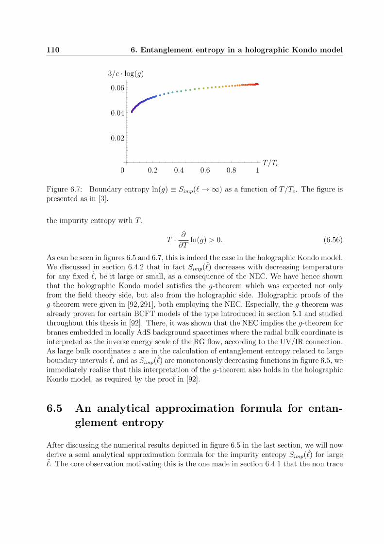
110 6. Entanglement entropy in a holographic Kondo model

3/c · log(g)

0.06

0.04

0.02

0 0.2 0.4 0.6 0.8 1T/Tc

Figure 6.7: Boundary entropy ln(g) ≡ Simp(` → ∞) as a function of T/Tc. The figure ispresented as in [3].

the impurity entropy with T ,

T · ∂∂T

ln(g) > 0. (6.56)

As can be seen in figures 6.5 and 6.7, this is indeed the case in the holographic Kondo model.We discussed in section 6.4.2 that in fact Simp(˜) decreases with decreasing temperaturefor any fixed ˜, be it large or small, as a consequence of the NEC. We have hence shownthat the holographic Kondo model satisfies the g-theorem which was expected not onlyfrom the field theory side, but also from the holographic side. Holographic proofs of theg-theorem were given in [92,291], both employing the NEC. Especially, the g-theorem wasalready proven for certain BCFT models of the type introduced in section 5.1 and studiedthroughout this thesis in [92]. There, it was shown that the NEC implies the g-theorem forbranes embedded in locally AdS background spacetimes where the radial bulk coordinate isinterpreted as the inverse energy scale of the RG flow, according to the UV/IR connection.As large bulk coordinates z are in the calculation of entanglement entropy related to largeboundary intervals ˜, and as Simp(˜) are monotonously decreasing functions in figure 6.5, weimmediately realise that this interpretation of the g-theorem also holds in the holographicKondo model, as required by the proof in [92].

6.5 An analytical approximation formula for entan-

glement entropy

After discussing the numerical results depicted in figure 6.5 in the last section, we will nowderive a semi analytical approximation formula for the impurity entropy Simp(˜) for large˜. The core observation motivating this is the one made in section 6.4.1 that the non trace

6.5 An analytical approximation formula for entanglement entropy 111

part of the energy-momentum tensor, SL/R, goes to zero both near the boundary and nearthe black hole event horizon. In this section, we will hence approximate the brane nearthe event horizon by fitting a constant tension brane (with SL/R = 0 for any z) to it asdepicted in figure 6.8.

horizon

brane

boundaryD(T )

fitted

x=

0

x(T

=Tc)

+(z

=z H

)

xT +

(z=z H

)

x(T

=Tc

)

+

(z)

x

z

xT+(z)

brane

Figure 6.8: Geometrical setup for the derivation of an analytical approximation formula forSimp(˜) for large ˜. Although all constant tension branes are curves of the form (6.40) in aBTZ background they are sketched as straight lines in this figure. This is justified becausefor the scale chosen e.g. in figure 6.4, the curvature of the constant tension solutions wouldnot be visible to the eye. For T < Tc, the brane with embedding profile xT+(z) asymptotesto xT=Tc

+ (z) near the boundary and can be approximated by a constant tension brane nearthe event horizon. This fitted brane will reach the boundary at the position x = −D. Thefigure is presented as in [3].

Such a constant tension brane will depend on only two parameters: its tension λ and theposition at which it is anchored at the AdS boundary, x ≡ −D. Constant tension solutionsand the way of constructing them via a geodesic normal flow were already discussed insection 5.3.1. Using the nomenclature suited for the study of the Kondo model in thissection, we can write equation (5.38) as

SλEE(`) = SBH(`) + C(λ). (6.57)

It should be noted however that this formula is only valid for intervals with length 2`symmetrically centered around the defect, which is supposed to be the point where thebrane meets the boundary. For convenience, this was chosen to be x = 0 so far, seee.g. figure 6.4. In figure 6.8 however, we see that the brane is anchored to the boundaryat x = −D, effectively broadening distance between the endpoint of the brane and theendpoints of the interval. The correct approximation formula thus reads

Sλ,DEE (`) = SBH(`+D) + C(λ). (6.58)

112 6. Entanglement entropy in a holographic Kondo model

Using this approximation as well as (6.50), the impurity entropy (6.51) can then be writtenas

Simp(`) = C(λ) +c

3log

(sinh (2πT (`+D))

sinh (2πT`)

)(6.59)

→ C(λ) +c

3

[2πTD +

(1− e−4πTD

)e−4πT` +O

(e−8πT`

)]for `T 1 (6.60)

∼ C(λ) +2πc

3TD

[1 + 2e−4πT` +O

(e−8πT`

)]for `T 1 and DT 1. (6.61)

As 4πT` = 2`/zH = 2˜, this semi-analytical approximation formula immediately explainsthe exponential falloff behaviour found in section 6.4.2 and seen in figure 6.6. Furthermore,the temperature dependent prefactor of the exponential falloff of the curves in figure 6.6 isidentified to be 1−e−4πTD by (6.60). This can indeed be checked to be true in our numericaldata. Equation (6.60) is hence already an important result, but as (6.61) indicates, thisinvestigation can be brought further by assuming D to be small compared to both ` andzH . We can then even write

Simp(`) = C(λ) + SBH(`+D)− SBH(`) (6.62)

≈ C(λ) +D · ∂`SBH(`) (6.63)

≈ C(λ(T )) +2πc

3TD(T ) coth (2πT`) for `T 1 and DT 1, (6.64)

thereby identifying the series expansion in (6.61) as the one of a coth.5 In (6.64) wehave reinstated that the temperature dependent fit-parameters λ and D are of course alsodependent on the temperature. Equation (6.64) lends itself to immediate comparison withthe field theory approximation formula [90]

Simp =π2c ξKT

6vcoth

(2π`T

v

)=π2c

6

T

TK

coth

(2π

`

ξK

T

TK

)for T/TK, ξK/` 1 (6.52)

in four aspects:

• First of all, the formula (6.64) includes the constant offset term C(λ) which is notpresent in (6.52). However, as λ is implicitly dependent on the temperature, it mayvanish for small T depending on the details of the model. We will have to saymore about the low temperature behaviour of the holographic Kondo model in theremainder of this section as well as in the next one.

• Secondly, we see that the arguments of the coth agree in both (6.64) and (6.52) ifthe Fermi velocity v is set equal to one, the speed of light, in the latter. This is

5Using a Poincare instead of a BTZ background we can derive a similar approximation formula for theT = 0 case. In particular, in this case SAdS(`) = c

3 log( 2`ε ) and D · ∂`SAdS(`) = cD

3` lead to a similar

formula to the zero-temperature result Simp = πc12

ξK` for ` ξK derived in [88–91]. Comparing this to

(6.52) respectively (6.64), we note that the limits T → 0 and `→∞ do not commute.

6.5 An analytical approximation formula for entanglement entropy 113

precisely the appropriate choice in the Kondo model as it is based on massless chiralfermions, see [86]. As is obvious from (6.60), the form of this argument determinesthe exponential falloff seen in section 6.4.2. In contrast to (6.52) which is valid forT/TK 1, this prediction of our geometrical analysis is expected to be valid for any(not necessarily small) temperature T , an expectation numerically verified by ourresults in figure 6.6.

• Thirdly, we can compare the prefactors of the coth terms in (6.64) and (6.52). Ifwe set v = 1 as discussed above, the comparison of these two factors suggests theidentification

D(T ) ≈ π

4ξK ⇔ D(T ) ≈ π2

2ξKT (6.65)

for small T , i.e. a proportionality between the geometric bulk length scale D and theKondo scale ξK .

• Lastly, an important aspect of the approximation formulas (6.64) and (6.52) thatshould be compared are their respective ranges of validity. In (6.64), we have statedthe condition

`T 1 and DT 1. (6.66)

This is necessary because the constant brane approximation depicted in figure 6.8only yields reliable results for the entanglement entropy when the bulk entanglingcurves meet the brane close to the event horizon, i.e. for `T 1. The conditionDT 1 is then necessary for the series (6.60) so simplify to (6.61), which is theseries expansion of the coth in (6.64). In contrast, (6.52) was derived in [90] underthe assumptions

T/TK 1 and ξK/` 1. (6.67)

Even with the identification D ∼ ξK ∼ 1/TK due to (6.65), we see that these setsof inequalities (6.66) and (6.67) are not equivalent. Specifically, while the conditionT/TK 1 is part of both (6.66) and (6.67), the condition involving ` differs betweenthe two as in (6.66) ` is compared to 1/T while in (6.67) it is compared to 1/TK .From (6.66) it can be shown that

T 1/` ⇒ ξK/` T/TK 1. (6.68)

This means that with the identification (6.65), (6.67) follows from (6.66), but (6.66)is stronger because it implies the additional hierarchy ξK/` T/TK .

Of course, the Kondo model studied in this chapter is only a bottom-up model, and ishence only expected to give qualitative insight into the properties of the “real” Kondoeffect, nevertheless it is interesting how (6.65) seems to suggest a connection between thelength scale ξK of the Kondo cloud and the geometrical quantity D defined in figure 6.8. In

114 6. Entanglement entropy in a holographic Kondo model

fact, the geometrical definition of D is so simple that in principle its approximate values canbe read off from figure 6.4 using a straight edge. It hence seems worthwhile to investigatethe possible relation (6.65) in more detail. Especially, we should investigate whether inour numerical solutions D(T ) becomes a linear function at low T . If this was the case, wecould argue that D(T = 0) is then a measure for the size ξK of the Kondo cloud, up to afactor of order one.

Unfortunately, this is not the case as the plot 6.9 of our numerical values of D(T ) shows.However, in order to assess this result we need to find out how the temperature T hasto be made before we can even expect a proportionality of the form (6.65). As we willnow show, there is an upper bound on the value of D(T ) in the holographic model, andconsequently, there is an upper bound on the temperatures T for which equation (6.65)can in principle hold. After all, we have stated before that (6.52) and similar formulas onlyhold for T/TK 1, but in the remainder of this section we will try to answer what the in this expression quantitatively means, i.e. how small is small enough in this context. Theargument for this is based on the fact that x+(zH) can only increase as T/Tc decreases.This can be seen in figure 6.4, and as discussed in sections 6.4.2 and 6.4.3, this is adirect consequence of the NEC being satisfied by the condensing scalar field. Furthermore,according to table 5.1 the violation of the SEC implies x′+(zH) < 0. Using these simplefacts, it then becomes clear from the sketch 6.8 that

D(T ) ≤ |x(T )+ (zH)| ≤ |x(T=Tc)

+ (zH)|. (6.69)

We know from sections 6.4.2 and 6.4.3 that the latter quantity is proportional to theboundary entropy in the uncondensed phase and using (6.53) this yields the bound

D(T ) ≤ |x(T=Tc)+ (zH)| = 3

cln(g(T=Tc)

)≈ 0.0626 (6.70)

for our numerics. The formula (6.65), predicting D(T ) to grow linearly with T for small Tcan hence at most be a good approximation to the behaviour of D(T ) until a temperatureT ∗ is reached at which the bound (6.70) is violated. Writing (6.65) as D(T ) ∼ const. T

Tc

with (using (6.37)) const. = π2Tc/(2TK) ≈ 4.37 this yields that the linear behaviour ofD(T ) can under no circumstances be seen for temperatures

T

Tc&T ∗

Tc≈ 0.014. (6.71)

This is however just a crude estimation, and realistically we would expect that we have togo orders of magnitude below (6.71) in order to numerically check the validity of relation(6.65) in the bottom-up model. See figure 6.9. Unfortunately, as this figure shows it wasnot possible to investigate the holographic Kondo model at low enough temperatures, dueto numerical problems. We can at the present time neither confirm nor exclude a behaviourof the form (6.65) in the holographic Kondo model. We will have to say more about thebehaviour of the holographic Kondo model at small temperatures in section 6.7.

6.5 An analytical approximation formula for entanglement entropy 115

D(T ) =π2 Tc

2TK· TTc ≈

4.37TTc

10−1

10−4

10−7

D(T )

10−5 10−4 10−3 10−2 10−1 1T/Tc

numericalresults

upper bound: D(T )∣∣∣x(T=Tc)

+ (zH)∣∣∣ = 3

clog(g(T=Tc)

)

expectation for a holographicmodel reproducing (6.52)

Linear behaviour has tostop before T/Tc ≈ 0.014

at low temperatures

Figure 6.9: The thick points represent the fitted values of D for various temperatures inour numerical results. The dotted line is a sketch of how the behaviour may look like in arealistic Kondo model that exactly reproduces (6.52) at low temperatures. We also indicatethe upper bound (6.70), the corresponding temperature bound (6.71) and a line indicatingthe expected small temperature behaviour D(T ) = π2

2TTK

. The figure is presented as in [3].

The bounds discussed in this section are in themselves an interesting result, as they con-strain the range of validity of approximation formulas for low temperatures in terms ofhigh temperature quantities such as 3

cln(g(T=Tc)

). In fact, the temperature bound (6.71)

that was derived from the bulk geometry of the holographic Kondo model can equivalentlybe derived purely in field theory terms. To do so, note that coth(x) → 1 as x → ∞. Theformula (6.52) would hence, if it were valid for any T , predict a linear increase of 3

cln(gT)

with T . However, by the g-theorem this quantity has to be bounded by 3c

ln(g(T=Tc)

),

leading to the realisation that (6.52) cannot be valid above temperatures (6.71).

To end this section, we should point out that although we were not able to numericallyinvestigate the holographic Kondo model at low enough temperatures, both results (6.52)and (6.64) are very general, and not dependent on specific properties of the Kondo system.In fact, (6.52) was derived in [90] by general CFT methods, and the derivation of (6.60)and (6.64) was based on the general geometrical properties of AdS/BCFT approaches ofthe type proposed in [92–94]. We hence expect that these results are universal in thesense that they can be applied to a large range of holographic models, irrespective of theirspecific details.

116 6. Entanglement entropy in a holographic Kondo model

6.6 An outlook on complexity

In chapter 3 we have outlined the deep holographic connection between entanglemententropy and bulk geometry. This connection has then be studied and employed in thelater chapter 4 as well as in sections 5.2.3 and 6.4.2-6.5. Now, we will look into anotherquantity related to quantum information in the field theory that can be, according to recentproposals [95–101], calculated from the bulk geometry. This quantity is computationalcomplexity.

Ideas relating to computational complexity seem to have entered gravitational physics indiscussions concerning the firewall paradox [293] in the works [95,294] where a connectionbetween complexity and bulk geometry was envisioned. See [295] for a review purelyfrom the quantum information theory point of view. Following the definition of [96] (seealso [95,98]), computational complexity is defined as the minimal number of simple unitaryoperations that have to be carried out by a quantum computer in order to implementa given unitary operation on a simple initial state, or to create a given state from asimple initial state. Based on the findings of [95,96], it was then suggested in [98,99] thatholographically, complexity C should be measured by the volumes V of certain spacelikecodimension one hypersurfaces, i.e.

C ∝ VLGN

. (6.72)

In the proposal of [99] for example, in a setup as depicted in figure 3.1, the complexity ofthe state of the subsystem A would be assumed to be proportional to the volume V of thespacelike hypersurface F . A proposal similar to (6.72) was made in [101] for a quantityreferred to as quantum information metric or fidelity susceptibility. Interestingly, the paper[101] also employed a thin brane ansatz similar to the AdS/BCFT models introducedin section 5.1, although they used spacelike branes Q. It was argued in [100, 296] thatcomputational complexity C should more accurately be calculated from the integral of thebulk action over a certain bulk region. However, the simple approximation formula (6.72)has continued to attract interest in the holography community, see [297–299].

In the above section 6.4.2, we dealt with entanglement entropy in the holographic Kondomodel, which is a divergent quantity regulated by the boundary cutoff ε. Impurity entropy(6.51) on the other hand was defined in such a way that the divergencies cancel and theleftover quantity is finite and has a well-defined physical meaning. We will now try toobtain a similar notion of impurity complexity, or as we will call it, relative complexityCrel. As we see from the definition (6.72), the complexity will be a divergent quantity dueto contributions from the part of the bulk spacetime near the boundary. To cancel thesecontributions, we define

Crel(T ) ∝ VT − VT=Tc , (6.73)

where VT is meant to be the volume of the (codimension one) equal time slices of our bulkgeometry. In short, we define the relative complexity to be proportional to the loss of bulk

6.6 An outlook on complexity 117

volume compared to T = Tc. We discussed in sections 6.4.1 and 6.4.2 that this loss of bulkvolume is a direct geometrical consequence of the NEC satisfied by the scalar field Φ. Theoverall sign is chosen such that Crel(T ) decreases with T , due to the hope that there mightbe a complexity analogue to the g-theorem discussed in section 6.4.3. The induced metricon an equal time slice of the BTZ black hole (5.17) reads

ds2 =1

z2

(dx2 +

dz2

1− z2

z2H

), (6.74)

and consequently we find

Crel(T ) ∝ VT − VT=Tc =

zH∫ε

dz1

z2√

1− z2

z2H

xT=Tc (z)∫xT (z)

dx (6.75)

=

zH∫ε

dzxT=Tc(z)− xT (z)

z2√

1− z2

z2H

. (6.76)

A priori, this quantity might be divergent in the limit ε → 06, but as we have discussedin section 6.4.1 and seen in figure 6.4, the scalar field on the branes falls off so fast nearthe boundary that the branes all approach z = 0 with the same leading (linear) behaviour.This then means that the quantity (6.76) is in fact finite, see figure 6.10 for a plot. Indeedwe see that Crel decreases monotonously along the RG flow, as expected. Whether this isrelated to the g-theorem or whether this is a general feature of holographic RG flows mightbe an interesting question for future research.

It should be noted that although Crel is finite in the holographic Kondo model, it is muchmore sensitive to the near-boundary behaviour of the branes than for example Simp(˜ 1):If the curves x(z) would not approach the boundary with the same slope x′(0), Simp wouldstill be a finite quantity, but Crel would not. This is due to the possible divergence of theintegral (6.76) at the lower bound ε→ 0, which does only not contribute due to the well-behaved near-boundary behaviour of the branes. The quantity (6.76) is also more sensitiveto the behaviour of the brane at intermediate values of 0 < z < zH than Simp(˜ 1).While our discussion in section 6.5 showed that the behaviour of Simp(˜) for large ˜ canbe described by an approximation formula only involving the two parameters C(λ) and D,no similar universal formula can be derived for Crel(T ). Although the idea of monitoringthe change of complexity along an RG flow is a qualitatively appealing one, the abovediscussion raises concerns about how useful the investigation of (relative) complexity willin practice be for the holographic study of RG flows. Especially, the absence of a universalapproximation formula for low temperatures is problematic, as in bottom-up AdS/CFT itare often the universal features of a system that are of interest, as they can be compared

6Near the event horizon the integrand also diverges, but only very mildly and consequently the integralconverges at the upper bound.

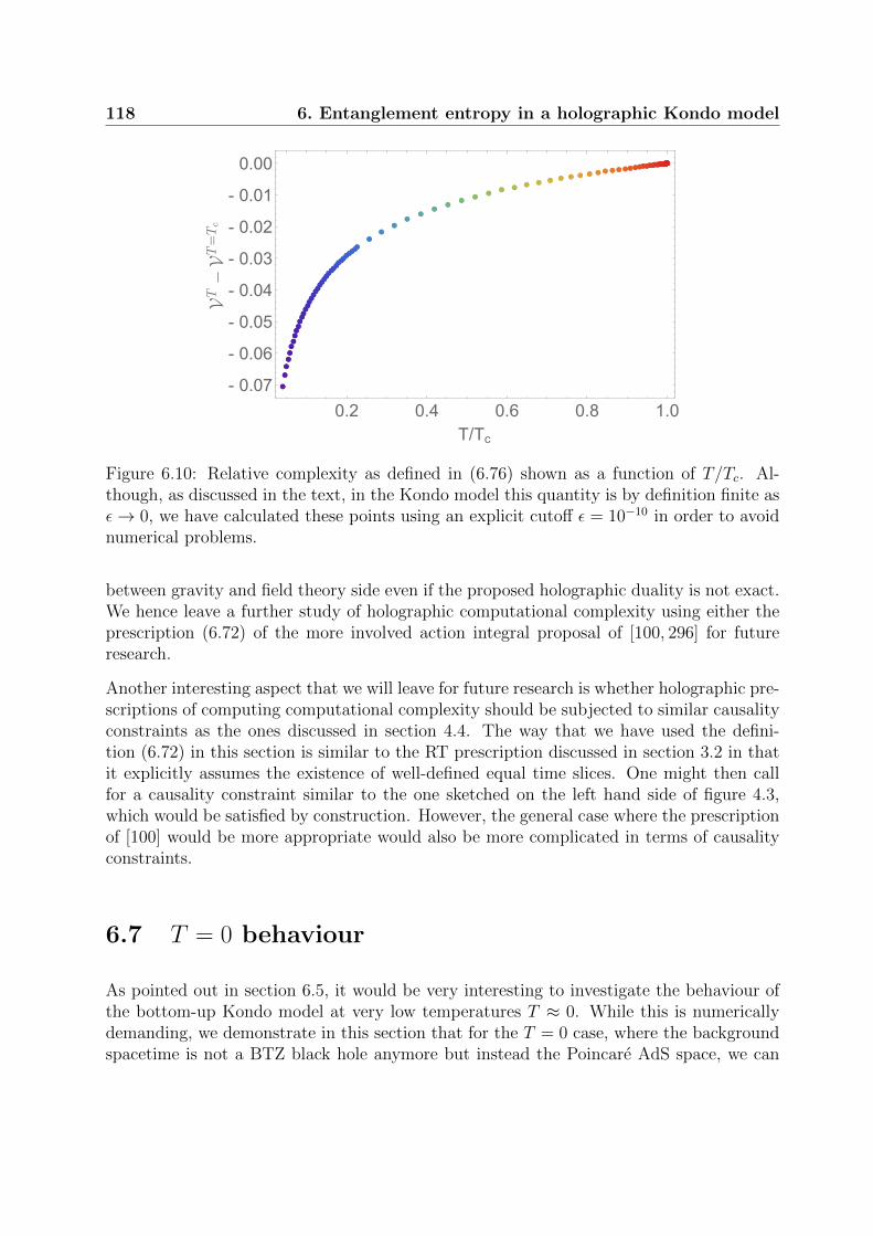
118 6. Entanglement entropy in a holographic Kondo model

0.2 0.4 0.6 0.8 1.0

- 0.07

- 0.06

- 0.05

- 0.04

- 0.03

- 0.02

- 0.01

0.00

T/Tc

Figure 6.10: Relative complexity as defined in (6.76) shown as a function of T/Tc. Al-though, as discussed in the text, in the Kondo model this quantity is by definition finite asε→ 0, we have calculated these points using an explicit cutoff ε = 10−10 in order to avoidnumerical problems.

between gravity and field theory side even if the proposed holographic duality is not exact.We hence leave a further study of holographic computational complexity using either theprescription (6.72) of the more involved action integral proposal of [100, 296] for futureresearch.

Another interesting aspect that we will leave for future research is whether holographic pre-scriptions of computing computational complexity should be subjected to similar causalityconstraints as the ones discussed in section 4.4. The way that we have used the defini-tion (6.72) in this section is similar to the RT prescription discussed in section 3.2 in thatit explicitly assumes the existence of well-defined equal time slices. One might then callfor a causality constraint similar to the one sketched on the left hand side of figure 4.3,which would be satisfied by construction. However, the general case where the prescriptionof [100] would be more appropriate would also be more complicated in terms of causalityconstraints.

6.7 T = 0 behaviour

As pointed out in section 6.5, it would be very interesting to investigate the behaviour ofthe bottom-up Kondo model at very low temperatures T ≈ 0. While this is numericallydemanding, we demonstrate in this section that for the T = 0 case, where the backgroundspacetime is not a BTZ black hole anymore but instead the Poincare AdS space, we can

6.7 T = 0 behaviour 119

use analytical arguments to assess the properties of the bottom-up model.

The specific question that we want to study is whether in the T = 0 case, our systemwill flow to an IR conformal fixed point. In an AdS/BCFT setting, this would mean thatdeep in the bulk spacetime we expect the brane to become effectively a constant tensionsolution [92–94], i.e.

Sij → const. · γij as z →∞ (6.77)

⇒ SL/R → 0 as z →∞. (6.78)

Due to our field theory intuition that a non-trivial scalar corresponds to the presence ofthe Kondo cloud, we will also make the assumption

⇒ φ→ const. 6= 0 as z →∞. (6.79)

Actually, in section 6.4.1 we saw that in the finite temperature T 6= 0 case we automaticallyget SL/R → 0 as z → zH as well as φ(zH) 6= 0, and as the zero-temperature limit is zH →∞,we might be tempted to take this as evidence that at T = 0 the behaviour (6.78), (6.79)indeed occurs. This, however, cannot be the case as we will now show.

To do so, we use the equation of motion (5.28) as well as the explicit expression for KL/Rgiven in table 5.1 to find that (6.78) and (6.78) necessarily imply the set of assumptionsthat, as z →∞,

KL/R =zx′′

2 (1 + x′2)3/2→ 0, (6.80)

⇒ x′′(z)→ 0 faster than z−1 ⇒ x′(z)→ const. (6.81)

Similarly, from the form of SL/R given in (6.35) and using that γij, defined in (5.23),behaves as ∼ z2 for large z, we find7

a0 → 0 faster than z−1, φ′ → 0 faster than z−1, (6.82)

where we already used the gauge choice of section 6.3.2. Let us now focus on the scalarequations of motion

∂m(√−γγmn∂nφ

)=√−γγ00a2

0φ+1

2

√−γ ∂V

∂φ. (6.83)

We will now assume that as z → ∞ and φ → const. 6= 0, the force term ∂V∂φ6= 0 which

is necessarily the case in the simple model (6.15). Due to the factor√−γ, the last term

in (6.83) will then, for large z, go to zero exactly as z−2 and consequently the equation

7As a technicality, we should note that for diagonal γmn, SL/R is a sum of two terms, but as γmn is bydefinition a positive definite matrix, these two terms cannot cancel each other. Hence when SL/R goes tozero, both terms compromising SL/R have to go to zero separately, yielding the above conditions.

120 6. Entanglement entropy in a holographic Kondo model

(6.83) can only be satisfied if there is another term that also goes as z−2 in this limit. Theconditions (6.81) and (6.82) however forbid precisely this: All the other terms in (6.83) canbe shown to approach zero strictly faster than z−2 for large z. We have hence demonstrateda contradiction between the equations of motion (6.83) and the assumptions (6.78) and(6.79), proving the assumptions wrong for simple ansatz (6.15).

There is a loophole in our argument, however. If we would choose a more complicatedpotential V such that for large z we find φ→ φ∗ and ∂V

∂φ

∣∣φ=φ∗

= 0, then a zero temperature

fixed point might exist. To obtain this result, we could for example add quartic or higherterms to the potential in (6.15). The model studied in this chapter so far would then bea good approximation to this more realistic model at higher temperatures T . Tc whereφ(z) stays comparably small, and only at lower temperatures T ≈ 0 where φ(z) attainslarger values for large z would the corrections to the potential become important. In thiscontext, we should note again that in the bottom-up model, the quadratic form (6.15) ofthe potential was in fact chosen purely for convenience. This is hence one of the featuresin where the bottom-up model deviates qualitatively from the top-down model discussedin section 6.1.2, and it should consequently not be surprising that one might need a moreintricate form of the potential to obtain more realistic results from the bottom-up modelat low temperatures.

Let us now try to gain as much insight into the desired properties of the potential V (φ) aspossible. What we already know is that there needs to be a φ∗ 6= 0 such that

∂φV∣∣φ=φ∗

= 0 , V∣∣φ=φ∗

≡ V ∗, (6.84)

i.e. there needs to be another extremum or saddle point away from φ = 0. But we can learnmore: The geometry that we would expect to get is one where near the boundary, as wellas deep in the bulk, the system is effectively described by constant tensions S = −2λi ≡Si, SL/R=0 (see section 5.3.1), and the brane interpolates between the two correspondingconstant tension solutions. By NEC and (5.31), we know that the traces have to increaseand by WEC they have to stay non-positive along the brane, hence

S1 < S2 ≤ 0, (6.85)

where S1 is the trace near the boundary (where φ falls off to zero) and S2 is the tracedeep in the bulk, for large z. These effective tensions receive different contributions. Asalready explained in section 6.4.1, near the boundary the main contribution comes fromthe a-field and its flux ∼ C2. Generally allowing for a non-zero V (φ = 0) ≡ V 0 (equivalentto a non-zero constant tension added to the brane) we find from equation (6.35):

S1 = −N(C2 + 2V 0

). (6.86)

Deep in the bulk in contrast, we assume the a-field to vanish because of (6.82), so that thetrace is

S2 = −2NV ∗. (6.87)

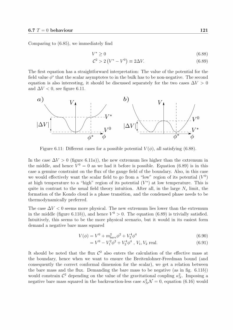
6.7 T = 0 behaviour 121

Comparing to (6.85), we immediately find

V ∗ ≥ 0 (6.88)

C2 > 2(V ∗ − V 0

)≡ 2∆V. (6.89)

The first equation has a straightforward interpretation: The value of the potential for thefield value φ∗ that the scalar asymptotes to in the bulk has to be non-negative. The secondequation is also interesting, it should be discussed separately for the two cases ∆V > 0and ∆V < 0, see figure 6.11.

Figure 6.11: Different cases for a possible potential V (φ), all satisfying (6.88).

In the case ∆V > 0 (figure 6.11a)), the new extremum lies higher than the extremum inthe middle, and hence V 0 = 0 as we had it before is possible. Equation (6.89) is in thiscase a genuine constraint on the flux of the gauge field of the boundary. Also, in this casewe would effectively want the scalar field to go from a “low” region of its potential (V 0)at high temperature to a “high” region of its potential (V ∗) at low temperature. This isquite in contrast to the usual field theory intuition. After all, in the large Ns limit, theformation of the Kondo cloud is a phase transition, and the condensed phase needs to bethermodynamically preferred.

The case ∆V < 0 seems more physical. The new extremum lies lower than the extremumin the middle (figure 6.11b)), and hence V 0 > 0. The equation (6.89) is trivially satisfied.Intuitively, this seems to be the more physical scenario, but it would in its easiest formdemand a negative bare mass squared

V (φ) = V 0 +m2bareφ

2 + V 42 φ

4 (6.90)

= V 0 − V 21 φ

2 + V 42 φ

4 , V1, V2 real. (6.91)

It should be noted that the flux C2 also enters the calculation of the effective mass atthe boundary, hence when we want to ensure the Breitenlohner-Freedman bound (andconsequently the correct conformal dimension for the scalar), we get a relation betweenthe bare mass and the flux. Demanding the bare mass to be negative (as in fig. 6.11b))would constrain C2 depending on the value of the gravitational coupling κ2

N . Imposing anegative bare mass squared in the backreaction-less case κ2

NN = 0, equation (6.16) would

122 6. Entanglement entropy in a holographic Kondo model

demand

Q2 = C2 <1

4. (6.92)

For finite values of κ2NN , this bound gets stricter. Setting κ2

NN = 1 for example, equation(6.44) and the imposition of a negative bare mass squared would lead to

C2 < 4

(√2−

√2√

2− 1

)≈ 0.248. (6.93)

This concludes our study of how to make the bottom-up Kondo model more realistic in thelower temperature regime by adding higher order terms to the potential V (φ). As we haveseen, this would have to be done under a number of strict constraints on the potential andthe asymptotic flux C. We leave a study of such a more realistic model and an investigationinto the physical meaning of the constraints derived above to the future.

Chapter 7

Outlook

It is now time to conclude our investigations into the geometrical properties of of entan-glement and defect entropies. In the introduction, we explained how gauge/gravity dualityoffers a concrete manifestation of the holographic principle, and even generally of the oldbelief that “physics is geometry”. We have then studied concrete formulations and re-alisations of holography in chapter 2, and the geometrical manifestation of entanglemententropy in chapter 3. The original results of the present author summarised in chapters4-6 were then consequently concerned with this topic of “entanglement from geometry”.

Entanglement entropy was studied in higher curvature theories in chapter 4. It is clearthat this is an ongoing research topic with steady progress, see [200, 201, 210, 225, 226]for only a partial list of work on this topic published after [1]. In particular, we dealtwith new massive gravity in section 4.2 and Gauss-Bonnet gravity in section 4.3. In bothcases we found unexpected solutions to the equations for the extremal surfaces that arethought to define holographic entanglement entropy. In section 4.4 we also pointed outthe importance of causality conditions such as the causal influence argument of [64]. Infact, causality conditions like this one are an important subject even in the absence ofhigher curvature corrections: If entanglement entropy (or another physical quantity ofthe boundary theory) is encoded in the bulk geometry in the form of extremal surfaces,it is of interest to find out which part of the bulk spacetime these surfaces have accessto [155]. This is related to the ongoing research into such topics as bulk locality and bulkreconstruction, [154–158], which we briefly commented on in the end of section 2.4.

Chapters 5 and 6 were then devoted to holographic models of AdS3/BCFT2 in general andof the Kondo effect in particular. Specifically, we were able to prove general theorems (insections 5.2.3 and 5.2.4) that restrict the possible qualitative features of the bulk geometry,depending on whether or not certain energy conditions are satisfied by the matter fields ofthe model. This, together with the study of exact solutions in section 5.3, gave us a veryfirm and intuitive understanding of the geometrical properties of the holographic Kondomodel, which we put to use in chapter 6. There, we presented numerical and semi-analytical

124 7. Outlook

results on the entanglement entropy in the holographic Kondo model (sections 6.4.2 and6.5), and compared them to field theory results obtained by Affleck et al. in [90] with goodagreement. We also verified that the holographic Kondo model satisfies the g-theorem,as expected, in section 6.4.3. Section 6.6 was devoted to the study of computationalcomplexity in the holographic Kondo model. Finally, the zero-temperature behaviour of themodel was investigated more closely in section 6.7, with clear suggestions for improvementsof the bottom-up model being made. This work presented in chapters 5 and 6 has openedup some fascinating possible avenues for future research on the junctions of geometry,gravity and quantum theory of impurities:

• As pointed out the introduction, AdS/CFT techniques have been applied to problemsin QCD with great success. Interestingly, it has been shown in [300] that a Kondo-like effect can occur in light quark matter, when heavy quarks act as impurities.This is a motivation to ask whether the results derived from the holographic Kondomodel of [86] can also be applied to the QCD Kondo effect, or whether a realisticholographic QCD-Kondo model can be constructed.

• In [301], the single impurity Kondo model has been described holographically interms of a multiscale entanglement renormalisation ansatz (MERA) network [302].In particular, the defect or impurity on the field theory side was holographicallydescribed by introducing boundary tensors into the tensor network. Assuming thatthe MERA construction leads to the emergence of an effective bulk geometry (asconjectured in [303]), these boundary tensors bear a striking resemblance to theboundary Q introduced into the bulk spacetime (see figure 5.1) in the holographicKondo model and similar models of a general AdS/BCFT duality. It would hencebe of great interest to compare the Kondo model with the one of [301], to find outwhether some of our results and techniques can be applied to the MERA model,and to investigate whether these two types of models are sharing a common physicalfoundation.

• One important part of our work presented in section 6.4.3 was the study of the g-theorem, proven in the holographic context already in [92,291]. Here, the g-function isa renormalisation group monotone for BCFTs, similar to the c-function for standardCFTs. We found in section 6.6 that the field theory RG flow manifested itself ina reduction of the volume of our bulk spacetime due to the loss of certain bulkpoints, and consequently via the Ryu-Takayanagi approach also in a reduction ofentanglement entropy. Indeed, entanglement entropy has been very successfully usedbefore to monitor RG flows e.g. in [46, 304]. The reduction of volume that is visiblein the holographic Kondo model on the other hand may be related, as explained insection 6.6, to measures of computational complexity or a quantum information metric[95–101]. It would certainly be interesting to investigate the interconnection betweenthe boundary RG flow, the loss of bulk points and quantities such as complexity inmore detail, as this might yield new insights about how the geometry emerges fromthe field theory side of the duality.

125

• Last but not least, in [86] it was pointed out that by using a higher spin theoryin the 2 + 1-dimensional bulk, it may be possible to construct a holographic modelthat is precisely dual to the large Ns Kondo effect, as this model has an infinitenumber of conserved currents of arbitrarily high spin. This may be a way around theusual pitfalls of a merely qualitative duality present in many bottom-up holographicmodels.

We hence see that there are many potential connections between the specific topics pre-sented in this thesis and the important current questions in AdS/CFT research. Withoutany doubt, the coming years will show a number of remarkable interconnections betweensuch diverse topics as (dynamical) geometry and quantum (information) theory.

Appendix A

Extrinsic curvature quantities

A.1 Codimension two hypersurfaces

As discussed in chapters 3 and 4, the holographic prescriptions for calculating entanglemententropy are based on the geometry of spacelike codimension two extremal hypersurfaces.In this appendix we will define some geometric quantities describing the extrinsic curvatureproperties of such a hypersurface. Specifically, we will clarify the notation (following [60,199]) used in equation (4.4) which shall be reproduced here for convenience:

SEE =1

4GN

∫Σ

dd−1y√γ

[1 + 2aR + b

(R‖ −

1

2k2

)+ 2c

(R‖‖ − Tr(k)2

)]. (4.4)

Here, Σ stands for a spacelike codimension-two hypersurface in a d + 1-dimensional bulkspacetime, y are the coordinates on this surface and its induced metric is γij with positivedeterminant γ. It is easy to see that in the case a = b = c = 0, (4.4) simplifies to thestandard area functional. We will now define the quantities R‖, R‖‖, k

2 and Tr(k)2. R isjust the standard Ricci scalar of the background spacetime gµν .

To begin, we will assume the background metric gµν to be Euclidean. The codimensiontwo hypersurface Σ will then have two spacelike normal vectors nµ(α) (α ∈ 1, 2) with

nµ(1)nν(1)gµν = nµ(2)n

ν(2)gµν = +1, nµ(1)n

ν(2)gµν = 0. (A.1)

R‖ and R‖‖ are derived from the background Ricci and Riemann tensors according to[60,199]

R‖ ≡ Rµν [g]nµ(α)nν(α), R‖‖ ≡ Rµρνσ[g]nµ(α)n

ν(α)n

ρ(β)n

σ(β), (A.2)

where we are summing over double bracketed Greek indices like (α). The extrinsic curva-

128 A. Extrinsic curvature quantities

ture terms k2 and Tr(k)2 can be defined according to [60] in the following way:

hµν = gµν − (n(α))µ(n(α))ν , (A.3)

k(α)µν = hλµh

ρν(n(α))λ;ρ, (A.4)

k2 = (k(α))µµ(k(α))νν , (A.5)

Tr(k)2 = (k(α))µν (k(α))νµ, (A.6)

where again summation over double indices like (α) is implied. In fact, we can imaginesuch indices to be contracted via a flat Euclidean metric δ(α)(β), although we do not usethe convention here that indices (α) are raised and lowered.

For Lorentzian background metrics gµν , we will effectively replace this by a Minkowskimetric η(α)(β). Specifically, we then get

nµ(1)nν(1)gµν = −1, nµ(2)n

ν(2)gµν = +1, nµ(1)n

ν(2)gµν = 0, (A.7)

R‖ ≡ Rµνnµ(α)n

ν(α) = −Rµνn

µ(1)n

ν(1) +Rµνn

µ(2)n

ν(2) (similarly for R‖‖), (A.8)

hµν = gµν + (n(1))µ(n(1))ν − (n(2))µ(n(2))ν , (A.9)

k(α)µν = hλµh

ρν(n(α))λ;ρ, (A.10)

k2 = −(k(1))µµ(k(1))νν + (k(2))µµ(k(2))νν , (A.11)

Tr(k)2 = −(k(1))µν (k(1))νµ + (k(2))µν (k(2))νµ. (A.12)

These definitions ensure that k2 and Tr(k)2 are independent of the choice of the nµ(α) as

long as nµ(1) is the timelike and nµ(2) is the spacelike normal vector.

A.2 Codimension one hypersurfaces

In the discussions of chapters 5 and 6 we deal with the embeddings of codimension onetimelike hypersurfaces into an asymptotically AdSd+1 ambient spacetime, as in [92–94]. Tobe specific, we are interested in the extrinsic curvature tensor or second fundamental form

Kij ≡∂Xα

∂ξi∂Xβ

∂ξj∇αnβ = −nα

(∂2Xα

∂ξi∂ξj+ Γαβγ

∂Xβ

∂ξi∂Xγ

∂ξj

), (A.13)

A.2 Codimension one hypersurfaces 129

where the Xα are the ambient space coordinates (α ∈ 0, ..., d), the ξi are the coordinateson the hypersurface (i ∈ 0, ..., d − 1) and nβ is the normal form of the hypersurface inthe ambient spacetime. Obviously, the sign of Kij needs to be fixed by a convention onthe direction of nβ. For one-sided models as the one described in section 5.1 we choose nβto be pointing into the spacetime, which is in contrast to the convention of [92–94]. Wechoose this convention because it is the more common one in two-sided models based onthe Israel junction conditions (6.28), such as the holographic Kondo model of section 6.2.There, for the equations of motion to take the form (6.29), the convention has to be thatthe normal form nβ points from the − side into the + side, as in figure 6.2.

The trace of the extrinsic curvature tensor can be straightforwardly defined by contractionwith the induced metric:

K = γijKij. (A.14)

Let us compare the expressions (A.13) and (A.14) with those presented in appendix A.1.Although the notation used here is a little bit different, we see that the underlying geometricideas are the same. Both in (A.13) and (A.4) respectively (A.10) we take the covariantderivative of the normal form and project it onto the worldvolume of the hypersurface inquestion. The difference is that firstly, in appendix A.1 we are dealing with codimension twohypersurfaces, hence there are two independent normal forms and two extrinsic curvaturescalars. Secondly, in appendix A.1 we have avoided introducing worldvolume coordinatesξi and their indices i. Hence, the induced metric (A.3) respectively (A.9) is effectively a(d+ 1)× (d+ 1) matrix, but a degenerate one. In contrast, the induced metric γij used inthis section and chapters 5 and 6 is a non-degenerate d× d matrix.

As a special case, in section 5.2.4 we calculate the extrinsic curvature tensor of a hyper-surface embedded into a background of the form (5.17). We assume ξ0 = X0 = t andξ1 = X2 = z, using the profile function x(t, z) to define the embedding of the hypersur-face into the ambient spacetime. The derivatives in (A.13) then simplify considerably.As the brane is defined by the embedding profile x(t, z), i.e. by viewing the x-coordinateas a function of the other coordinates, it is located at the set of zeros of the functionf(t, z, x) ≡ x− x(t, z). The normal form nµ is then proportional (up to its normalisation)to the exterior derivative of f :

nµdxµ ∼ df = dx− ∂tx(t, z)dt− ∂zx(t, z)dz. (A.15)

Raising the index and calculating the normalisation, we explicitly find

nµ =z2

N

∂txh

−h∂zx1

, (A.16)

N = z

√1− (∂tx)2

h+ h (∂zx)2, (A.17)

130 A. Extrinsic curvature quantities

where the order of bulk coordinates is chosen to be t, z, x. The extrinsic curvature tensoris

K±tt =1

N

(−∂ 2

t x+ ∂zx

(h

2

(h′ − 2h

z

)+h

z(∂tx)2

)),

K±tz = Kzt =1

N

(−∂t∂zx+ ∂tx

(h

z(∂zx)2 +

h′

2h

)),

K±zz =1

N

(−∂ 2

z x+ ∂zx

(h

z(∂zx)2 +

1

z− h′

2h

)),

(A.18)

and the induced metric reads

γij =

(gtt + (∂tx)2 gxx (∂tx) (∂zx) gxx(∂tx) (∂zx) gxx gzz + (∂zx)2 gxx

). (A.19)

In the last expression, we made use of the fact that (5.17) is a diagonal metric.

Appendix B

Corollary to the barrier theorem inhigher dimensions

This appendix will be devoted to discussing an extension of our findings of section 5.2.3to higher dimensions. This is non-trivial, but also potentially useful for model buildingpurposes. For example, in [243] a holographic model of the quantum Hall effect waspresented using the AdS/BCFT ansatz (5.1) with a 3 + 1-dimensional bulk spacetime.There, it was argued (see especially figure 2(d) of [243]) that in a realistic model, thebranes should bend back to the boundary in a ∪-shaped manner. A better understandingof the implications of the barrier theorem on AdS/BCFT models in higher dimensionsmight then enable for a more efficient model building yielding such a desired behaviour.

First of all, we see that our results of section 5.2.3 cannot be straightforwardly carried overto higher dimensions as it is possible to construct explicit examples of codimension onebranes in 3 + 1-dimensional Poincare space that satisfy both WEC and SEC and yet donot satisfy (5.14). We do not have analytical results on the energy conditions needed toensure (5.14) in higher dimensions, but by studying a large number of randomly generatedenergy-momentum tensors1 for 2+1-dimensional branes obeying (5.2) we found that (5.14)is ensured by the SEC (generalised to higher dimensions compared to (5.11)) together withthe dominant energy condition (DEC, [246, 247]) and the determinant energy condition(DetEC, [247, 305]). The generalisation of the ∪-shaped branes encountered in sections5.2.3 and 5.3.2 are then bowl shaped surfaces, as sketched on the left hand side of figureB.1.

However, for the phenomenological purposes of [243] one does not need bowl-shaped hy-persurfaces, but such ones which are anchored at the boundary in the form of an infinitestrip. Such surfaces cannot satisfy the barrier theorem, as shown in figure B.1. But if it

1Note that the condition (5.14) as well as all energy conditions are pointwise conditions, i.e. they donot depend on derivatives of Sij or Kij . Hence we can check them at any point on the brane separately,and Sij can then be treated as a symmetric matrix with numerical entries.

132 B. Corollary to the barrier theorem in higher dimensions

Figure B.1: Left: A bowl shaped hypersurface, anchored to the boundary in a circle. Thetime direction is omitted in this sketch, u and v are spacelike coordinates on the asymptoticboundary and z is the bulk coordinate, as in Poincare coordinates. Right: A surface that isanchored on the boundary in a strip-like geometry is not an extremal hypersurface barrierin the sense of section 5.2.3 as it can e.g. be crossed by a geodesic shown as Υ in the figure.Nevertheless, a section of this in the v = const. plane yields a ∪-shaped profile. The figureis presented as in [2].

was possible to formulate the barrier theorem only for curves in the z, u-plane, the barriertheorem might tell us how to choose the matter content on the brane such that a ∪-shapedprofile in the z, u-plane is inevitable. This is what we will study in the remainder of thisappendix.

Assuming a strip-like setup for the brane defined by the profile function U(z) as in theright hand side of figure B.1 and a 3+1-dimensional Poincare background spacetime (2.11)with L = 1, the extrinsic curvature reads (coordinates x0 = t, x1 = z, x2 = v)

Kαβ =

− u′(z)

z2√

1+u′(z)20 0

0 u′(z)+u′(z)3−zu′′(z)z2√

1+u′(z)20

0 0 u′(z)

z2√

1+u′(z)2

. (B.1)

Comparing this to (5.18), we can map this to the lower dimensional case by realising thatthe first two entries on the diagonal of (B.1) are the extrinsic curvature of a brane withprofile u(z) embedded in 2 + 1-dimensional Poincare space. Comparing this then to theresults in table 5.1 we see that, apart from the trivial case u′(z) = 0, u(z) has to be ∪-shaped when u′(z) ≥ 0 and u′(z) + u′(z)3 − zu′′(z) ≤ 0 hold2. This automatically impliesKyy ≥ 0 and hence a violation of (5.14) for spacelike vectors vi in y-direction. Hence,extremal curves moving in the y-direction such as Υ in figure B.1 may cross the brane.

2Note that, due to our convention on the orientation of the normal vector, these expressions only holdfor the one branch of the brane that goes into the bulk up to the turning point.

133

Setting κ2N = 1 for simplicity, we find from (5.2) that

Sαβ =

−2(u′+u′3)−zu′′

z2(1+u′2)3/2 0 0

0 2u′√

1+u′2

z2 0

0 0 −−2(u′+u′3)+zu′′

z2(1+u′2)3/2

. (B.2)

As we are only interested in establishing the brane to be an extremal surface barrier inthe u-z-plane, we will in the following only use vectors with vanishing v-component. TheNEC then implies u′′ ≥ 0, the WEC implies the NEC together with 2u′ + 2u′3 − zu′′ ≤ 0and consequently u′′ ≥ 0, WEC implies 2u′ + 2u′3 − zu′′ ≤ 0 and together, these imply

u′ + u′3 − zu′′ ≤ 0. (B.3)

This expression also appears in the zz-component of (B.1). Projecting out the v-componentfrom the tensors above yields

K⊥ij =

(− u′

z2√

1+u′20

0 u′+u′3−zu′′z2√

1+u′2

), (B.4)

S⊥ij =

−2(u′+u′3)−zu′′

z2(1+u′2)3/2 0

0 2u′√

1+u′2

z2

, (B.5)

γ⊥ij =

(− 1z2 0

0 1+u′2

z2

). (B.6)

If we then replace the SEC with the inequality(S⊥ij − γ⊥ijS⊥

)vivj ≥ 0, (B.7)

with S⊥ = γ⊥ijS⊥ij , we get the familiar condition u′(z) ≥ 0 which together with the WECensures that K⊥ij is negative definite. If the matter fields living on the brane are chosen tosatisfy the given energy conditions, the branes necessarily have a ∪-shaped profile u(z) inthe v = const. plane, as desired in [243].

Appendix C

Junction conditions for abelianChern-Simons fields

The bottom-up Kondo model described in section 6.2 had two fields defined in the entirebulk spacetime (N in the nomenclature of figure 5.1), namely the metric gµν and theAbelian Chern-Simons (CS) field Aµ. At the locus of the brane, the metric needs to satisfythe Israel junction conditions, as discussed in section 6.3.1. Similarly, junction conditionshave to be imposed on the CS field, and we will derive these junction conditions in thissection. Just as for the Israel junction conditions, there are several ways how to do this,and here we will follow the ansatz of starting with a smoothed out worldvolume current,and then take the limit in which the current is localised at a codimension one hypersurface.This is somewhat related to the study of domain wall solutions in CS theories, see [306,307].

To begin, we assume that we are working in a Gaussian normal coordinate system, suchthat the brane is located at x = 0. In the holographic Kondo model, the current is definedby the charged scalar Φ = φ eiψ and reads

Jm = γmn i(ΦDnΦ† − Φ†DnΦ

)= 2 γmn (An − an + ∂nψ)φ2 , (C.1)

which we can write as Jm ∼ Q(z) (∂t)m in the static case. As depicted in figure C.1, we

now assume the current to be smoothed out by a profile function f(x) with stem-functionF (x), such that there exists a well-defined limit in which f(x)→ δ(x), F (x)→ θ(x). Here,δ(x) is the Dirac delta distribution and θ(x) is the Heaviside step function.

Due to our assumption of staticity, all time-derivatives vanish, and hence the CS equationsof motion,

ερµνFµν = −4π Jρ, (C.2)

have only the non-trivial component

2 εtz (∂zAx − ∂xAz) = −4π J t = −4π f(x)Q(z). (C.3)

136 C. Junction conditions for abelian Chern-Simons fields

z

tx

Jµ = δµt f(x)Q(z)

C

x = 0

Figure C.1: The static worldvolume current of a brane located at x = 0 is assumed to besmoothed out to have a bell-shaped profile f(x). A possible Wilson loop is depicted as C.The figure is presented as in [3].

The worldvolume ε-tensor appearing in this equation is defined from the three-dimensionalε-tensor via contracting with the normal form of the brane. In Gaussian normal coordi-nates, this reads ερµx ≡ ερµ. We can now solve (C.3) in two simple ways, depending on agauge choice:

Gauge Ax = 0: With this gauge, we find

−εtz∂xAz = −2π f(x)Q(z) , (C.4)

⇒ εtzAz = 2π F (x)Q(z) . (C.5)

Taking the limit F → Θ, f → δ, these equations then tell us that the parallel componentof the CS field has a discontinuity proportional to the charge density Q on the brane.

Gauge A′z = 0: To distinguish this gauge from the one used above, we add primes to theCS field. A′z = 0 leads to

εtz∂zA′x = −2π f(x)Q(z) (C.6)

⇒ −εtzA′x = 2π f(x)

z∫0

√−γQ(z) dz , (C.7)

where ε denotes the Levi-Civita symbol, which is related to the Levi-Civita tensor byεmn = εmn/

√−γ(z). The limit F → Θ, f → δ then implies that the component of

the Chern-Simons field normal to the brane acquires a contribution ∼ δ(x) in this gaugeconvention.

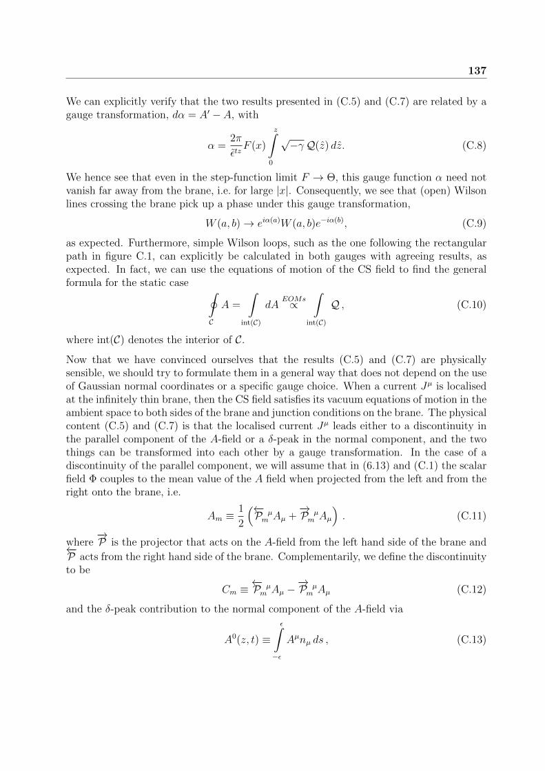
137

We can explicitly verify that the two results presented in (C.5) and (C.7) are related by agauge transformation, dα = A′ − A, with

α =2π

εtzF (x)

z∫0

√−γQ(z) dz. (C.8)

We hence see that even in the step-function limit F → Θ, this gauge function α need notvanish far away from the brane, i.e. for large |x|. Consequently, we see that (open) Wilsonlines crossing the brane pick up a phase under this gauge transformation,

W (a, b)→ eiα(a)W (a, b)e−iα(b), (C.9)

as expected. Furthermore, simple Wilson loops, such as the one following the rectangularpath in figure C.1, can explicitly be calculated in both gauges with agreeing results, asexpected. In fact, we can use the equations of motion of the CS field to find the generalformula for the static case ∮

C

A =

∫int(C)

dAEOMs∝

∫int(C)

Q , (C.10)

where int(C) denotes the interior of C.

Now that we have convinced ourselves that the results (C.5) and (C.7) are physicallysensible, we should try to formulate them in a general way that does not depend on the useof Gaussian normal coordinates or a specific gauge choice. When a current Jµ is localisedat the infinitely thin brane, then the CS field satisfies its vacuum equations of motion in theambient space to both sides of the brane and junction conditions on the brane. The physicalcontent (C.5) and (C.7) is that the localised current Jµ leads either to a discontinuity inthe parallel component of the A-field or a δ-peak in the normal component, and the twothings can be transformed into each other by a gauge transformation. In the case of adiscontinuity of the parallel component, we will assume that in (6.13) and (C.1) the scalarfield Φ couples to the mean value of the A field when projected from the left and from theright onto the brane, i.e.

Am ≡1

2

(←−P µm Aµ +

−→P µm Aµ

). (C.11)

where−→P is the projector that acts on the A-field from the left hand side of the brane and←−

P acts from the right hand side of the brane. Complementarily, we define the discontinuityto be

Cm ≡←−P µm Aµ −

−→P µm Aµ (C.12)

and the δ-peak contribution to the normal component of the A-field via

A0(z, t) ≡ε∫

−ε

Aµnµ ds , (C.13)

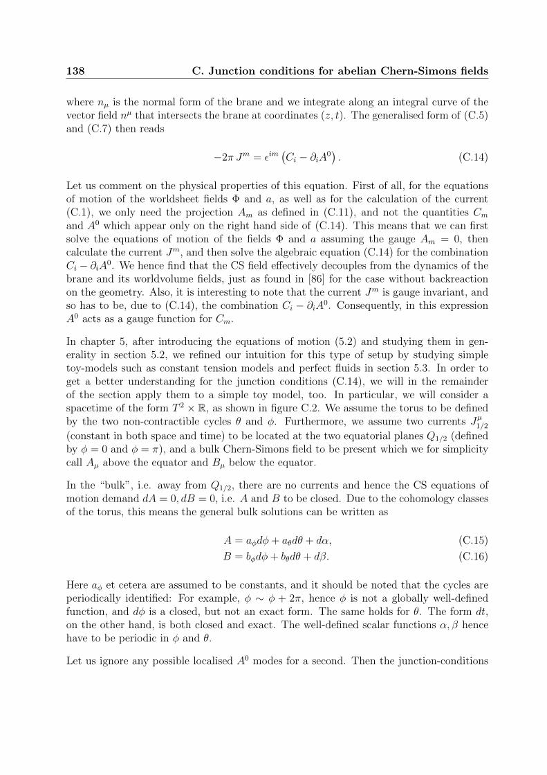
138 C. Junction conditions for abelian Chern-Simons fields

where nµ is the normal form of the brane and we integrate along an integral curve of thevector field nµ that intersects the brane at coordinates (z, t). The generalised form of (C.5)and (C.7) then reads

−2π Jm = εim(Ci − ∂iA0

). (C.14)

Let us comment on the physical properties of this equation. First of all, for the equationsof motion of the worldsheet fields Φ and a, as well as for the calculation of the current(C.1), we only need the projection Am as defined in (C.11), and not the quantities Cmand A0 which appear only on the right hand side of (C.14). This means that we can firstsolve the equations of motion of the fields Φ and a assuming the gauge Am = 0, thencalculate the current Jm, and then solve the algebraic equation (C.14) for the combinationCi − ∂iA0. We hence find that the CS field effectively decouples from the dynamics of thebrane and its worldvolume fields, just as found in [86] for the case without backreactionon the geometry. Also, it is interesting to note that the current Jm is gauge invariant, andso has to be, due to (C.14), the combination Ci − ∂iA0. Consequently, in this expressionA0 acts as a gauge function for Cm.

In chapter 5, after introducing the equations of motion (5.2) and studying them in gen-erality in section 5.2, we refined our intuition for this type of setup by studying simpletoy-models such as constant tension models and perfect fluids in section 5.3. In order toget a better understanding for the junction conditions (C.14), we will in the remainderof the section apply them to a simple toy model, too. In particular, we will consider aspacetime of the form T 2 × R, as shown in figure C.2. We assume the torus to be definedby the two non-contractible cycles θ and φ. Furthermore, we assume two currents Jµ1/2(constant in both space and time) to be located at the two equatorial planes Q1/2 (definedby φ = 0 and φ = π), and a bulk Chern-Simons field to be present which we for simplicitycall Aµ above the equator and Bµ below the equator.

In the “bulk”, i.e. away from Q1/2, there are no currents and hence the CS equations ofmotion demand dA = 0, dB = 0, i.e. A and B to be closed. Due to the cohomology classesof the torus, this means the general bulk solutions can be written as

A = aφdφ+ aθdθ + dα, (C.15)

B = bφdφ+ bθdθ + dβ. (C.16)

Here aφ et cetera are assumed to be constants, and it should be noted that the cycles areperiodically identified: For example, φ ∼ φ + 2π, hence φ is not a globally well-definedfunction, and dφ is a closed, but not an exact form. The same holds for θ. The form dt,on the other hand, is both closed and exact. The well-defined scalar functions α, β hencehave to be periodic in φ and θ.

Let us ignore any possible localised A0 modes for a second. Then the junction-conditions

139

Figure C.2: A simple toy model for the illustration of the junction conditions for theChern-Simons field. We assume the bulk space to be a three dimensional space with thetopology T 2 ×R, and two charge distributions to be confined to the two equatorial circlesof the torus.

Cm ∝ εmnJn give

aθ − bθ + ∂θα− ∂θβ∣∣Q1

= J t1, (C.17)

bθ − aθ − ∂θα + ∂θβ∣∣Q2

= J t2, (C.18)

where we have set a numerical proportionality constant to one. We see that if there isa time component in the current, we get a θ component in the jump Cm. While Jtdtis topologically trivial, const. · dθ is an element of a non-trivial cohomology class of thetorus. Being in a different cohomology class, the terms ∂α can hence not contribute to thesolution and the previous equations read

aθ − bθ = J t1, ∂θα− ∂θβ∣∣Q1

= 0, (C.19)

bθ − aθ = J t2, ∂θα− ∂θβ∣∣Q2

= 0. (C.20)

For the currents, this means

J t1 = −J t2, (C.21)

i.e. the total charge on the torus has to vanish. This is a result that we would expect on anyspace with closed spacial sections, also for Maxwell theory for example. Due to dt beingan exact form, we do not get these topological complications for the equations involvingJθ1/2, and hence there is no restriction on these components (if time is not compactified).It makes sense that the constraints between J1/2 that are conveyed by the CS field onlyconcern conserved charges which have to be fixed once: As the CS field has no propagatingdegrees of freedom, it cannot communicate dynamical information from Q1 to Q2.

We claimed above that the addition of the term ∼ ∂mA0 in the junction condition restores a

sense of gauge freedom for Cm. This may be correct on topologically simpler backgrounds,

140 C. Junction conditions for abelian Chern-Simons fields

but in this example it would not be possible to gauge away the jump Cm, as again ∂mA0

would be in the wrong cohomology class to make Cm vanish.

Bibliography

[1] J. Erdmenger, M. Flory, and C. Sleight, “Conditions on holographic entanglingsurfaces in higher curvature gravity,” JHEP 06 (2014) 104, arXiv:1401.5075[hep-th].

[2] J. Erdmenger, M. Flory, and M.-N. Newrzella, “Bending branes for DCFT in twodimensions,” JHEP 01 (2015) 058, arXiv:1410.7811 [hep-th].

[3] J. Erdmenger, M. Flory, C. Hoyos, M.-N. Newrzella, and J. M. S. Wu,“Entanglement Entropy in a Holographic Kondo Model,” Fortsch. Phys. 64 (2016)109–130, arXiv:1511.03666 [hep-th].

[4] J. Erdmenger, M. Flory, C. Hoyos, M.-N. Newrzella, A. O’Bannon, and J. Wu,“Holographic impurities and Kondo effect,” in The String Theory Universe, 21stEuropean String Workshop and 3rd COST MP1210 Meeting Leuven, Belgium,September 7-11, 2015. 2015. arXiv:1511.09362 [hep-th].

[5] LIGO Scientific Collaboration and Virgo Collaboration, “Observation ofgravitational waves from a binary black hole merger,” Phys. Rev. Lett. 116 (Feb,2016) 061102.

[6] A. Pais, Raffiniert ist der Herrgott...: Albert Einstein. Eine wissenschaftlicheBiographie. Spektrum Akademischer Verlag, Heidelberg, 2009.

[7] J. A. Wheeler, “Geons,” Phys. Rev. 97 (Jan, 1955) 511–536.

[8] J. A. Wheeler and C. W. Misner, “Classical physics as geometry,” Ann. Phys. 2(1957) 525–603.

[9] J. Maldacena and L. Susskind, “Cool horizons for entangled black holes,” Fortsch.Phys. 61 (2013) 781–811, arXiv:1306.0533 [hep-th].

[10] K. Jensen and A. Karch, “Holographic Dual of an Einstein-Podolsky-Rosen Pairhas a Wormhole,” Phys. Rev. Lett. 111 no. 21, (2013) 211602, arXiv:1307.1132[hep-th].

[11] K. Jensen and J. Sonner, “Wormholes and entanglement in holography,” Int. J.Mod. Phys. D23 no. 12, (2014) 1442003, arXiv:1405.4817 [hep-th].

142 BIBLIOGRAPHY

[12] D. Engelhardt, B. Freivogel, and N. Iqbal, “Electric fields and quantumwormholes,” Phys. Rev. D92 no. 6, (2015) 064050, arXiv:1504.06336 [hep-th].

[13] N. Bao, J. Pollack, and G. N. Remmen, “Splitting Spacetime and Cloning Qubits:Linking No-Go Theorems across the ER=EPR Duality,” Fortsch. Phys. 63 (2015)705–710, arXiv:1506.08203 [hep-th].

[14] J. D. Bekenstein, “Black holes and the second law,” Lett. Nuovo Cim. 4 (1972)737–740.

[15] J. D. Bekenstein, “Black holes and entropy,” Phys. Rev. D7 (1973) 2333–2346.

[16] J. D. Bekenstein, “Generalized second law of thermodynamics in black holephysics,” Phys. Rev. D9 (1974) 3292–3300.

[17] J. D. Bekenstein, “A Universal Upper Bound on the Entropy to Energy Ratio forBounded Systems,” Phys. Rev. D23 (1981) 287.

[18] G. ’t Hooft, “Dimensional reduction in quantum gravity,” in Salamfest1993:0284-296, pp. 0284–296. 1993. arXiv:gr-qc/9310026 [gr-qc].

[19] L. Susskind, “The World as a hologram,” J. Math. Phys. 36 (1995) 6377–6396,arXiv:hep-th/9409089 [hep-th].

[20] R. Blumenhagen, D. Lust, and S. Theisen, Basic concepts of string theory.Springer, Heidelberg, Germany, 2013.

[21] M. B. Green, J. H. Schwarz, and E. Witten, SUPERSTRING THEORY. VOL. 1:INTRODUCTION. Cambridge University Press, Cambridge, UK, 1988.

[22] M. B. Green, J. H. Schwarz, and E. Witten, SUPERSTRING THEORY. VOL. 2:LOOP AMPLITUDES, ANOMALIES AND PHENOMENOLOGY. CambridgeUniversity Press, Cambridge, UK, 1988.

[23] J. Polchinski, String theory. Vol. 1: An introduction to the bosonic string.Cambridge University Press, Cambridge, UK, 2007.

[24] J. Polchinski, String theory. Vol. 2: Superstring theory and beyond. CambridgeUniversity Press, Cambridge, UK, 2007.

[25] J. M. Maldacena, “The Large N limit of superconformal field theories andsupergravity,” Int. J. Theor. Phys. 38 (1999) 1113–1133, arXiv:hep-th/9711200[hep-th]. [Adv. Theor. Math. Phys.2,231(1998)].

[26] S. S. Gubser, I. R. Klebanov, and A. M. Polyakov, “Gauge theory correlators fromnoncritical string theory,” Phys. Lett. B428 (1998) 105–114,arXiv:hep-th/9802109 [hep-th].

[27] E. Witten, “Anti-de Sitter space and holography,” Adv. Theor. Math. Phys. 2(1998) 253–291, arXiv:hep-th/9802150 [hep-th].

BIBLIOGRAPHY 143

[28] D. A. Lowe and L. Thorlacius, “AdS / CFT and the information paradox,” Phys.Rev. D60 (1999) 104012, arXiv:hep-th/9903237 [hep-th].

[29] P. Kovtun, D. T. Son, and A. O. Starinets, “Viscosity in strongly interactingquantum field theories from black hole physics,” Phys. Rev. Lett. 94 (2005) 111601,arXiv:hep-th/0405231 [hep-th].

[30] D. T. Son and A. O. Starinets, “Viscosity, Black Holes, and Quantum FieldTheory,” Ann. Rev. Nucl. Part. Sci. 57 (2007) 95–118, arXiv:0704.0240[hep-th].

[31] S. Bhattacharyya, V. E. Hubeny, S. Minwalla, and M. Rangamani, “NonlinearFluid Dynamics from Gravity,” JHEP 02 (2008) 045, arXiv:0712.2456 [hep-th].

[32] M. Rangamani, “Gravity and Hydrodynamics: Lectures on the fluid-gravitycorrespondence,” Class. Quant. Grav. 26 (2009) 224003, arXiv:0905.4352[hep-th].

[33] J. Casalderrey-Solana, H. Liu, D. Mateos, K. Rajagopal, and U. A. Wiedemann,“Gauge/String Duality, Hot QCD and Heavy Ion Collisions,” arXiv:1101.0618

[hep-th].

[34] M. Luzum and P. Romatschke, “Conformal Relativistic Viscous Hydrodynamics:Applications to RHIC results at s(NN)**(1/2) = 200-GeV,” Phys. Rev. C78 (2008)034915, arXiv:0804.4015 [nucl-th]. [Erratum: Phys. Rev.C79,039903(2009)].

[35] J. D. Edelstein, J. P. Shock, and D. Zoakos, “The AdS/CFT Correspondence andNon-perturbative QCD,” AIP Conf. Proc. 1116 (2009) 265–284, arXiv:0901.2534[hep-ph].

[36] O. DeWolfe, S. S. Gubser, C. Rosen, and D. Teaney, “Heavy ions and stringtheory,” Prog. Part. Nucl. Phys. 75 (2014) 86–132, arXiv:1304.7794 [hep-th].

[37] J. Sonnenschein, “Holography Inspired Stringy Hadrons,” arXiv:1602.00704

[hep-th].

[38] J. Erdmenger, N. Evans, I. Kirsch, and E. Threlfall, “Mesons in Gauge/GravityDuals - A Review,” Eur. Phys. J. A35 (2008) 81–133, arXiv:0711.4467 [hep-th].

[39] F. Brunner and A. Rebhan, “Nonchiral enhancement of scalar glueball decay in thewitten-sakai-sugimoto model,” Phys. Rev. Lett. 115 (Sep, 2015) 131601.

[40] S. S. Gubser, “Breaking an Abelian gauge symmetry near a black hole horizon,”Phys. Rev. D78 (2008) 065034, arXiv:0801.2977 [hep-th].

[41] S. A. Hartnoll, C. P. Herzog, and G. T. Horowitz, “Building a HolographicSuperconductor,” Phys. Rev. Lett. 101 (2008) 031601, arXiv:0803.3295[hep-th].

[42] A. G. Green, “An Introduction to Gauge Gravity Duality and Its Application in

144 BIBLIOGRAPHY

Condensed Matter,” Contemp. Phys. 54 no. 1, (2013) 33, arXiv:1304.5908[cond-mat.str-el].

[43] D. Musso, “Introductory notes on holographic superconductors,” PoSModave2013 (2013) 004, arXiv:1401.1504 [hep-th].

[44] L. Susskind and E. Witten, “The Holographic bound in anti-de Sitter space,”arXiv:hep-th/9805114 [hep-th].

[45] D. Z. Freedman, S. S. Gubser, K. Pilch, and N. P. Warner, “Renormalization groupflows from holography supersymmetry and a c theorem,” Adv. Theor. Math. Phys.3 (1999) 363–417, arXiv:hep-th/9904017 [hep-th].

[46] R. C. Myers and A. Sinha, “Holographic c-theorems in arbitrary dimensions,”JHEP 01 (2011) 125, arXiv:1011.5819 [hep-th].

[47] R. C. Myers and A. Sinha, “Seeing a c-theorem with holography,” Phys. Rev. D82(2010) 046006, arXiv:1006.1263 [hep-th].

[48] D. L. Jafferis, I. R. Klebanov, S. S. Pufu, and B. R. Safdi, “Towards theF-Theorem: N=2 Field Theories on the Three-Sphere,” JHEP 06 (2011) 102,arXiv:1103.1181 [hep-th].

[49] H. Casini and M. Huerta, “On the RG running of the entanglement entropy of acircle,” Phys. Rev. D85 (2012) 125016, arXiv:1202.5650 [hep-th].

[50] L. Susskind and J. Lindesay, An introduction to black holes, information and thestring theory revolution: The holographic universe. World Scientific Publishing,Hackensack, USA, 2005.

[51] M. Ammon and J. Erdmenger, Gauge/gravity duality. Cambridge Univ. Pr.,Cambridge, UK, 2015.

[52] H. Nastase, Introduction to the ADS/CFT Correspondence. Cambridge UniversityPress, Cambridge, UK, 2015.

[53] M. Natsuume, “AdS/CFT Duality User Guide,” Lect. Notes Phys. 903 (2015)pp.1–294, arXiv:1409.3575 [hep-th].

[54] M. Nielsen and I. Chuang, Quantum Computation and Quantum Information: 10thAnniversary Edition. Cambridge University Press, Cambridge, UK, 2010.

[55] S. Ryu and T. Takayanagi, “Holographic derivation of entanglement entropy fromAdS/CFT,” Phys. Rev. Lett. 96 (2006) 181602, arXiv:hep-th/0603001 [hep-th].

[56] S. Ryu and T. Takayanagi, “Aspects of Holographic Entanglement Entropy,” JHEP08 (2006) 045, arXiv:hep-th/0605073 [hep-th].

[57] R. M. Wald, “Black hole entropy is the Noether charge,” Phys. Rev. D48 (1993)3427–3431, arXiv:gr-qc/9307038 [gr-qc].

BIBLIOGRAPHY 145

[58] T. Jacobson, G. Kang, and R. C. Myers, “On black hole entropy,” Phys. Rev. D49(1994) 6587–6598, arXiv:gr-qc/9312023 [gr-qc].

[59] V. Iyer and R. M. Wald, “Some properties of Noether charge and a proposal fordynamical black hole entropy,” Phys. Rev. D50 (1994) 846–864,arXiv:gr-qc/9403028 [gr-qc].

[60] D. V. Fursaev, A. Patrushev, and S. N. Solodukhin, “Distributional Geometry ofSquashed Cones,” Phys. Rev. D88 no. 4, (2013) 044054, arXiv:1306.4000[hep-th].

[61] R.-X. Miao, “A Note on Holographic Weyl Anomaly and Entanglement Entropy,”Class. Quant. Grav. 31 (2014) 065009, arXiv:1309.0211 [hep-th].

[62] X. Dong, “Holographic Entanglement Entropy for General Higher DerivativeGravity,” JHEP 01 (2014) 044, arXiv:1310.5713 [hep-th].

[63] J. Camps, “Generalized entropy and higher derivative Gravity,” JHEP 03 (2014)070, arXiv:1310.6659 [hep-th].

[64] M. Headrick, V. E. Hubeny, A. Lawrence, and M. Rangamani, “Causality &holographic entanglement entropy,” JHEP 12 (2014) 162, arXiv:1408.6300[hep-th].

[65] J. Kondo, “Resistance minimum in dilute magnetic alloys,” Progress of TheoreticalPhysics 32 no. 1, (1964) 37–49.

[66] L. Kouwenhoven and L. Glazman, “Revival of the Kondo effect,”arXiv:cond-mat/0104100.

[67] A. C. Hewson and J. Kondo, “Kondo effect,” Scholarpedia 4 no. 3, (2009) 7529.revision #91408.

[68] J. Kondo, “Sticking to my bush,” Journal of the Physical Society of Japan 74 no. 1,(2005) 1–3.

[69] D. K. C. MacDonald, W. B. Pearson, and I. M. Templeton, “Thermo-electricity atlow temperatures. ix. the transition metals as solute and solvent,” Proceedings ofthe Royal Society of London A: Mathematical, Physical and Engineering Sciences266 no. 1325, (1962) 161–184.

[70] K. G. Wilson, “The renormalization group: Critical phenomena and the kondoproblem,” Rev. Mod. Phys. 47 (Oct, 1975) 773–840.

[71] P. W. Anderson, “A poor man’s derivation of scaling laws for the kondo problem,”Journal of Physics C: Solid State Physics 3 no. 12, 2436.

[72] H. Ishii, “Spin correlation in dilute magnetic alloys,” Journal of Low TemperaturePhysics 32 no. 3, 457–467.

146 BIBLIOGRAPHY

[73] E. S. Sørensen and I. Affleck, “Scaling theory of the kondo screening cloud,” Phys.Rev. B 53 (Apr, 1996) 9153–9167.

[74] I. Affleck, “The Kondo screening cloud: what it is and how to observe it,” ArXive-prints (Nov., 2009) , arXiv:0911.2209 [cond-mat.mes-hall].

[75] L. Kouwenhoven and C. Marcus, “Quantum dots,” Physics World 11 no. 6, 35.

[76] S. Kachru, A. Karch, and S. Yaida, “Holographic Lattices, Dimers, and Glasses,”Phys. Rev. D81 (2010) 026007, arXiv:0909.2639 [hep-th].

[77] S. Kachru, A. Karch, and S. Yaida, “Adventures in Holographic Dimer Models,”New J. Phys. 13 (2011) 035004, arXiv:1009.3268 [hep-th].

[78] S. Harrison, S. Kachru, and G. Torroba, “A maximally supersymmetric Kondomodel,” Class. Quant. Grav. 29 (2012) 194005, arXiv:1110.5325 [hep-th].

[79] N. Karaiskos, K. Sfetsos, and E. Tsatis, “Brane embeddings in spheresubmanifolds,” Class. Quant. Grav. 29 (2012) 025011, arXiv:1106.1200[hep-th].

[80] K. Jensen, S. Kachru, A. Karch, J. Polchinski, and E. Silverstein, “Towards aholographic marginal Fermi liquid,” Phys. Rev. D84 (2011) 126002,arXiv:1105.1772 [hep-th].

[81] A. Faraggi and L. A. Pando Zayas, “The Spectrum of Excitations of HolographicWilson Loops,” JHEP 05 (2011) 018, arXiv:1101.5145 [hep-th].

[82] A. Faraggi, W. Mueck, and L. A. Pando Zayas, “One-loop Effective Action of theHolographic Antisymmetric Wilson Loop,” Phys. Rev. D85 (2012) 106015,arXiv:1112.5028 [hep-th].

[83] P. Benincasa and A. V. Ramallo, “Fermionic impurities in Chern-Simons-mattertheories,” JHEP 02 (2012) 076, arXiv:1112.4669 [hep-th].

[84] G. Itsios, K. Sfetsos, and D. Zoakos, “Fermionic impurities in the unquenchedABJM,” JHEP 01 (2013) 038, arXiv:1209.6617 [hep-th].

[85] P. Benincasa and A. V. Ramallo, “Holographic Kondo Model in VariousDimensions,” JHEP 06 (2012) 133, arXiv:1204.6290 [hep-th].

[86] J. Erdmenger, C. Hoyos, A. O’Bannon, and J. Wu, “A Holographic Model of theKondo Effect,” JHEP 12 (2013) 086, arXiv:1310.3271 [hep-th].

[87] A. O’Bannon, I. Papadimitriou, and J. Probst, “A Holographic Two-ImpurityKondo Model,” JHEP 01 (2016) 103, arXiv:1510.08123 [hep-th].

[88] E. S. Sørensen, M.-S. Chang, N. Laflorencie, and I. Affleck, “Impurity entanglemententropy and the kondo screening cloud,” Journal of Statistical Mechanics: Theoryand Experiment 2007 no. 01, L01001.

BIBLIOGRAPHY 147

[89] I. Affleck, N. Laflorencie, and E. S. Sørensen, “Entanglement entropy in quantumimpurity systems and systems with boundaries,” Journal of Physics A:Mathematical and Theoretical 42 no. 50, 504009.

[90] E. S. Sørensen, M.-S. Chang, N. Laflorencie, and I. Affleck, “Quantum impurityentanglement,” Journal of Statistical Mechanics: Theory and Experiment 2007no. 08, P08003.

[91] E. Eriksson and H. Johannesson, “Impurity entanglement entropy in kondo systemsfrom conformal field theory,” Phys. Rev. B 84 (Jul, 2011) 041107.

[92] T. Takayanagi, “Holographic Dual of BCFT,” Phys. Rev. Lett. 107 (2011) 101602,arXiv:1105.5165 [hep-th].

[93] M. Fujita, T. Takayanagi, and E. Tonni, “Aspects of AdS/BCFT,” JHEP 11 (2011)043, arXiv:1108.5152 [hep-th].

[94] M. Nozaki, T. Takayanagi, and T. Ugajin, “Central Charges for BCFTs andHolography,” JHEP 06 (2012) 066, arXiv:1205.1573 [hep-th].

[95] L. Susskind, “Butterflies on the Stretched Horizon,” arXiv:1311.7379 [hep-th].

[96] L. Susskind, “Computational Complexity and Black Hole Horizons,” Fortsch. Phys.64 (2016) 24–43, arXiv:1402.5674 [hep-th].

[97] L. Susskind, “Addendum to Computational Complexity and Black Hole Horizons,”arXiv:1403.5695 [hep-th].

[98] L. Susskind, “Entanglement is not enough,” Fortsch. Phys. 64 (2016) 49–71,arXiv:1411.0690 [hep-th].

[99] M. Alishahiha, “Holographic Complexity,” Phys. Rev. D92 no. 12, (2015) 126009,arXiv:1509.06614 [hep-th].

[100] A. R. Brown, D. A. Roberts, L. Susskind, B. Swingle, and Y. Zhao, “ComplexityEquals Action,” arXiv:1509.07876 [hep-th].

[101] M. Miyaji, T. Numasawa, N. Shiba, T. Takayanagi, and K. Watanabe, “Distancebetween Quantum States and Gauge-Gravity Duality,” Phys. Rev. Lett. 115 no. 26,(2015) 261602, arXiv:1507.07555 [hep-th].

[102] M. Visser, Lorentzian wormholes: From Einstein to Hawking. AIP Press,Woodbury, USA, 1995.

[103] J. D. Brown and M. Henneaux, “Central Charges in the Canonical Realization ofAsymptotic Symmetries: An Example from Three-Dimensional Gravity,” Commun.Math. Phys. 104 (1986) 207–226.

[104] R. Bousso, “The Holographic principle,” Rev. Mod. Phys. 74 (2002) 825–874,arXiv:hep-th/0203101 [hep-th].

148 BIBLIOGRAPHY

[105] R. M. Wald, General Relativity. Chicago Univ. Pr., Chicago, USA, 1984.

[106] S. W. Hawking, “Black hole explosions,” Nature 248 (1974) 30–31.

[107] S. W. Hawking, “Particle Creation by Black Holes,” Commun. Math. Phys. 43(1975) 199–220.

[108] J. M. Bardeen, B. Carter, and S. W. Hawking, “The Four laws of black holemechanics,” Commun. Math. Phys. 31 (1973) 161–170.

[109] S. W. Hawking, “Gravitational radiation from colliding black holes,” Phys. Rev.Lett. 26 (1971) 1344–1346.

[110] S. W. Hawking, “Black holes in general relativity,” Commun. Math. Phys. 25(1972) 152–166.

[111] R. D. Sorkin, R. M. Wald, and Z. J. Zhang, “Entropy of selfgravitating radiation,”Gen. Rel. Grav. 13 (1981) 1127–1146.

[112] W. G. Unruh and R. M. Wald, “Acceleration Radiation and Generalized SecondLaw of Thermodynamics,” Phys. Rev. D25 (1982) 942–958.

[113] S. Hawking and R. Penrose, The Nature of space and time. Princeton Univ. Pr.,Princeton, USA, 1996.

[114] V. P. Frolov and I. D. Novikov, eds., Black hole physics: Basic concepts and newdevelopments. Kluwer Academic, Dordrecht, Netherlands, 1998.

[115] L. Smolin, “Lessons from Einstein’s 1915 discovery of general relativity,”arXiv:1512.07551 [physics.hist-ph].

[116] G. t. Hooft, “The Cellular Automaton Interpretation of Quantum Mechanics. AView on the Quantum Nature of our Universe, Compulsory or Impossible?,”arXiv:1405.1548 [quant-ph].

[117] T. Padmanabhan, “Gravity and/is Thermodynamics,” Curr. Sci. 109 (2015)2236–2242, arXiv:1512.06546 [gr-qc].

[118] T. Padmanabhan, “Exploring the Nature of Gravity,” 2016. arXiv:1602.01474[gr-qc].

[119] R. Goswami and G. F. R. Ellis, “The holographic principle in general relativity: thecase of Petrov type D vacuum spacetimes,” arXiv:1511.05700 [gr-qc].

[120] R. Bousso, “A Covariant entropy conjecture,” JHEP 07 (1999) 004,arXiv:hep-th/9905177 [hep-th].

[121] V. Faraoni, “Cosmological and Black Hole Apparent Horizons,” Lect. Notes Phys.907 (2015) pp.1–199.

[122] R. Bousso, “Holography in general space-times,” JHEP 06 (1999) 028,

BIBLIOGRAPHY 149

arXiv:hep-th/9906022 [hep-th].

[123] S. Carlip, Quantum gravity in 2+1 dimensions. Cambridge University Press,Cambridge, UK, 2003.

[124] O. Coussaert, M. Henneaux, and P. van Driel, “The Asymptotic dynamics ofthree-dimensional Einstein gravity with a negative cosmological constant,” Class.Quant. Grav. 12 (1995) 2961–2966, arXiv:gr-qc/9506019 [gr-qc].

[125] A. Strominger, “Black hole entropy from near horizon microstates,” JHEP 02(1998) 009, arXiv:hep-th/9712251 [hep-th].

[126] V. Balasubramanian and P. Kraus, “A Stress tensor for Anti-de Sitter gravity,”Commun. Math. Phys. 208 (1999) 413–428, arXiv:hep-th/9902121 [hep-th].

[127] P. Kraus, “Lectures on black holes and the AdS(3) / CFT(2) correspondence,”Lect. Notes Phys. 755 (2008) 193–247, arXiv:hep-th/0609074 [hep-th].

[128] S. J. van Albada, “Boundary Dynamics of Three-Dimensional AsymptoticallyAnti-de Sitter Space-Times,” arXiv:1601.07055 [hep-th].

[129] W. Li, W. Song, and A. Strominger, “Chiral Gravity in Three Dimensions,” JHEP04 (2008) 082, arXiv:0801.4566 [hep-th].

[130] M. Banados, M. Henneaux, C. Teitelboim, and J. Zanelli, “Geometry of the (2+1)black hole,” Phys. Rev. D48 (1993) 1506–1525, arXiv:gr-qc/9302012 [gr-qc].[Erratum: Phys. Rev.D88,069902(2013)].

[131] M. Banados, C. Teitelboim, and J. Zanelli, “The Black hole in three-dimensionalspace-time,” Phys. Rev. Lett. 69 (1992) 1849–1851, arXiv:hep-th/9204099[hep-th].

[132] R. Blumenhagen and E. Plauschinn, “Introduction to conformal field theory,” Lect.Notes Phys. 779 (2009) 1–256.

[133] O. Aharony, S. S. Gubser, J. M. Maldacena, H. Ooguri, and Y. Oz, “Large N fieldtheories, string theory and gravity,” Phys. Rept. 323 (2000) 183–386,arXiv:hep-th/9905111 [hep-th].

[134] E. D’Hoker and D. Z. Freedman, “Supersymmetric gauge theories and the AdS /CFT correspondence,” in Strings, Branes and Extra Dimensions: TASI 2001:Proceedings, pp. 3–158. 2002. arXiv:hep-th/0201253 [hep-th].

[135] J. McGreevy, “Holographic duality with a view toward many-body physics,” Adv.High Energy Phys. 2010 (2010) 723105, arXiv:0909.0518 [hep-th].

[136] J. Polchinski, “Introduction to Gauge/Gravity Duality,” in Proceedings, TheoreticalAdvanced Study Institute in Elementary Particle Physics (TASI 2010). StringTheory and Its Applications: From meV to the Planck Scale: Boulder, Colorado,USA, June 1-25, 2010, pp. 3–46. 2010. arXiv:1010.6134 [hep-th].

150 BIBLIOGRAPHY

[137] A. V. Ramallo, “Introduction to the AdS/CFT correspondence,” Springer Proc.Phys. 161 (2015) 411–474, arXiv:1310.4319 [hep-th].

[138] V. E. Hubeny, “The AdS/CFT Correspondence,” Class. Quant. Grav. 32 no. 12,(2015) 124010, arXiv:1501.00007 [gr-qc].

[139] S. de Haro, D. R. Mayerson, and J. Butterfield, “Conceptual Aspects ofGauge/Gravity Duality,” arXiv:1509.09231 [physics.hist-ph].

[140] J. Dai, R. G. Leigh, and J. Polchinski, “New Connections Between StringTheories,” Mod. Phys. Lett. A4 (1989) 2073–2083.

[141] J. Polchinski, “Dirichlet Branes and Ramond-Ramond charges,” Phys. Rev. Lett.75 (1995) 4724–4727, arXiv:hep-th/9510017 [hep-th].

[142] E. Kiritsis, String theory in a nutshell. Princeton Univ. Pr., Princeton, USA, 2007.

[143] O. Aharony and E. Witten, “Anti-de Sitter space and the center of the gaugegroup,” JHEP 11 (1998) 018, arXiv:hep-th/9807205 [hep-th].

[144] G. Hooft, “A planar diagram theory for strong interactions,” Nuclear Physics B 72no. 3, (1974) 461 – 473.

[145] S. Weinberg and E. Witten, “Limits on Massless Particles,” Phys. Lett. B96 (1980)59.

[146] S. de Haro, S. N. Solodukhin, and K. Skenderis, “Holographic reconstruction ofspace-time and renormalization in the AdS / CFT correspondence,” Commun.Math. Phys. 217 (2001) 595–622, arXiv:hep-th/0002230 [hep-th].

[147] K. Skenderis, “Lecture notes on holographic renormalization,” Class. Quant. Grav.19 (2002) 5849–5876, arXiv:hep-th/0209067 [hep-th].

[148] O. Aharony, O. Bergman, D. L. Jafferis, and J. Maldacena, “N=6 superconformalChern-Simons-matter theories, M2-branes and their gravity duals,” JHEP 10(2008) 091, arXiv:0806.1218 [hep-th].

[149] T. Sakai and S. Sugimoto, “Low energy hadron physics in holographic QCD,” Prog.Theor. Phys. 113 (2005) 843–882, arXiv:hep-th/0412141 [hep-th].

[150] T. Sakai and S. Sugimoto, “More on a holographic dual of QCD,” Prog. Theor.Phys. 114 (2005) 1083–1118, arXiv:hep-th/0507073 [hep-th].

[151] R. Collier, C. Burkhardt, and L. Lin, Optical Holography. Academic Press, NewYork, USA, 1971.

[152] L. Bergmann, H. Niedrig, and H. Eichler, Optik: Wellen- und Teilchenoptik. deGruyter, Berlin, 2004.

[153] D. V. Khveshchenko, “Contrasting string holography to its optical namesake,”Europhys. Lett. 109 (2015) 61001, arXiv:1411.1693 [cond-mat.str-el].

BIBLIOGRAPHY 151

[154] A. Almheiri, X. Dong, and D. Harlow, “Bulk Locality and Quantum ErrorCorrection in AdS/CFT,” JHEP 04 (2015) 163, arXiv:1411.7041 [hep-th].

[155] B. Freivogel, R. A. Jefferson, L. Kabir, B. Mosk, and I.-S. Yang, “Casting Shadowson Holographic Reconstruction,” Phys. Rev. D91 no. 8, (2015) 086013,arXiv:1412.5175 [hep-th].

[156] E. Mintun, J. Polchinski, and V. Rosenhaus, “Bulk-Boundary Duality, GaugeInvariance, and Quantum Error Corrections,” Phys. Rev. Lett. 115 no. 15, (2015)151601, arXiv:1501.06577 [hep-th].

[157] F. Pastawski, B. Yoshida, D. Harlow, and J. Preskill, “Holographic quantumerror-correcting codes: Toy models for the bulk/boundary correspondence,” JHEP06 (2015) 149, arXiv:1503.06237 [hep-th].

[158] X. Dong, D. Harlow, and A. C. Wall, “Bulk Reconstruction in the EntanglementWedge in AdS/CFT,” arXiv:1601.05416 [hep-th].

[159] T. Nishioka, S. Ryu, and T. Takayanagi, “Holographic Entanglement Entropy: AnOverview,” J. Phys. A42 (2009) 504008, arXiv:0905.0932 [hep-th].

[160] S. Ghosh, R. M. Soni, and S. P. Trivedi, “On The Entanglement Entropy ForGauge Theories,” JHEP 09 (2015) 069, arXiv:1501.02593 [hep-th].

[161] H. Araki and E. H. Lieb, “Entropy inequalities,” Commun. Math. Phys. 18 (1970)160–170.

[162] P. Calabrese and J. L. Cardy, “Entanglement entropy and quantum field theory,”J. Stat. Mech. 0406 (2004) P06002, arXiv:hep-th/0405152 [hep-th].

[163] D. V. Fursaev, “Proof of the holographic formula for entanglement entropy,” JHEP09 (2006) 018, arXiv:hep-th/0606184 [hep-th].

[164] M. Headrick and T. Takayanagi, “A Holographic proof of the strong subadditivityof entanglement entropy,” Phys. Rev. D76 (2007) 106013, arXiv:0704.3719[hep-th].

[165] M. Headrick, “Entanglement Renyi entropies in holographic theories,” Phys. Rev.D82 (2010) 126010, arXiv:1006.0047 [hep-th].

[166] A. Lewkowycz and J. Maldacena, “Generalized gravitational entropy,” JHEP 08(2013) 090, arXiv:1304.4926 [hep-th].

[167] T. Faulkner, “The Entanglement Renyi Entropies of Disjoint Intervals inAdS/CFT,” arXiv:1303.7221 [hep-th].

[168] T. Hartman, “Entanglement Entropy at Large Central Charge,” arXiv:1303.6955

[hep-th].

[169] V. E. Hubeny, M. Rangamani, and T. Takayanagi, “A Covariant holographic

152 BIBLIOGRAPHY

entanglement entropy proposal,” JHEP 07 (2007) 062, arXiv:0705.0016[hep-th].

[170] V. E. Hubeny, H. Maxfield, M. Rangamani, and E. Tonni, “Holographicentanglement plateaux,” JHEP 08 (2013) 092, arXiv:1306.4004 [hep-th].

[171] A. C. Wall, “Maximin Surfaces, and the Strong Subadditivity of the CovariantHolographic Entanglement Entropy,” Class. Quant. Grav. 31 no. 22, (2014)225007, arXiv:1211.3494 [hep-th].

[172] M. Headrick, “General properties of holographic entanglement entropy,” JHEP 03(2014) 085, arXiv:1312.6717 [hep-th].

[173] J. M. Maldacena, “Eternal black holes in anti-de Sitter,” JHEP 04 (2003) 021,arXiv:hep-th/0106112 [hep-th].

[174] E. Witten, “Anti-de Sitter space, thermal phase transition, and confinement ingauge theories,” Adv. Theor. Math. Phys. 2 (1998) 505–532,arXiv:hep-th/9803131 [hep-th].

[175] M. Mezard, G. Parisi, and M. Virasoro, Spin Glass Theory and Beyond. No. Nr.1993 in Lecture Notes in Physics Series. World Scientific, New Jersey, USA, 1987.

[176] L.-Y. Hung, R. C. Myers, and M. Smolkin, “On Holographic Entanglement Entropyand Higher Curvature Gravity,” JHEP 04 (2011) 025, arXiv:1101.5813 [hep-th].

[177] J. de Boer, M. Kulaxizi, and A. Parnachev, “Holographic Entanglement Entropy inLovelock Gravities,” JHEP 07 (2011) 109, arXiv:1101.5781 [hep-th].

[178] E. A. Bergshoeff, O. Hohm, and P. K. Townsend, “Massive Gravity in ThreeDimensions,” Phys. Rev. Lett. 102 (2009) 201301, arXiv:0901.1766 [hep-th].

[179] E. A. Bergshoeff, O. Hohm, and P. K. Townsend, “More on Massive 3D Gravity,”Phys. Rev. D79 (2009) 124042, arXiv:0905.1259 [hep-th].

[180] Y. Liu and Y.-w. Sun, “Note on New Massive Gravity in AdS(3),” JHEP 04 (2009)106, arXiv:0903.0536 [hep-th].

[181] D. Grumiller and O. Hohm, “AdS(3)/LCFT(2): Correlators in New MassiveGravity,” Phys. Lett. B686 (2010) 264–267, arXiv:0911.4274 [hep-th].

[182] Y. Liu and Y.-W. Sun, “Consistent Boundary Conditions for New Massive Gravityin AdS3,” JHEP 05 (2009) 039, arXiv:0903.2933 [hep-th].

[183] U. Camara dS, C. P. Constantinidis, and G. M. Sotkov, “New Massive GravityHolography,” Int. J. Mod. Phys. A28 (2013) 1350073, arXiv:1009.2665[hep-th].

[184] A. Sinha, “On the new massive gravity and AdS/CFT,” JHEP 06 (2010) 061,arXiv:1003.0683 [hep-th].

BIBLIOGRAPHY 153

[185] B. Chen, J.-j. Zhang, J.-d. Zhang, and D.-l. Zhong, “Aspects of WarpedAdS3/CFT2 Correspondence,” JHEP 04 (2013) 055, arXiv:1302.6643 [hep-th].

[186] M. Alishahiha, A. F. Astaneh, and M. R. M. Mozaffar, “Entanglement Entropy forLogarithmic Conformal Field Theory,” Phys. Rev. D89 no. 6, (2014) 065023,arXiv:1310.4294 [hep-th].

[187] B. Chen, F.-y. Song, and J.-j. Zhang, “Holographic Renyi entropy in AdS3/LCFT2

correspondence,” JHEP 03 (2014) 137, arXiv:1401.0261 [hep-th].

[188] S. Deser, R. Jackiw, and S. Templeton, “Topologically Massive Gauge Theories,”Annals Phys. 140 (1982) 372–411.

[189] S. Deser, R. Jackiw, and S. Templeton, “Three-Dimensional Massive GaugeTheories,” Phys. Rev. Lett. 48 (1982) 975–978.

[190] E. A. Bergshoeff, S. de Haan, O. Hohm, W. Merbis, and P. K. Townsend,“Zwei-Dreibein Gravity: A Two-Frame-Field Model of 3D Massive Gravity,” Phys.Rev. Lett. 111 no. 11, (2013) 111102, arXiv:1307.2774. [Erratum: Phys. Rev.Lett.111,no.25,259902(2013)].

[191] M. Banados, C. Deffayet, and M. Pino, “The Boulware-Deser mode in 3Dfirst-order massive gravity,” Phys. Rev. D88 no. 12, (2013) 124016,arXiv:1310.3249 [hep-th].

[192] E. A. Bergshoeff, O. Hohm, W. Merbis, A. J. Routh, and P. K. Townsend,“Chern-Simons-like Gravity Theories,” Lect. Notes Phys. 892 (2015) 181–201,arXiv:1402.1688 [hep-th].

[193] M. R. Setare and H. Adami, “On the new version of Generalized Zwei-DreibeinGravity,” Phys. Lett. B750 (2015) 31–36, arXiv:1508.00120 [hep-th].

[194] E. Bergshoeff, O. Hohm, W. Merbis, A. J. Routh, and P. K. Townsend, “MinimalMassive 3D Gravity,” Class. Quant. Grav. 31 (2014) 145008, arXiv:1404.2867[hep-th].

[195] A. S. Arvanitakis and P. K. Townsend, “Minimal Massive 3D Gravity UnitarityRedux,” Class. Quant. Grav. 32 no. 8, (2015) 085003, arXiv:1411.1970 [hep-th].

[196] M. R. Setare, “On the Generalized Minimal Massive Gravity,” Nucl. Phys. B898(2015) 259–275, arXiv:1412.2151 [hep-th].

[197] P. Breitenlohner and D. Z. Freedman, “Stability in Gauged ExtendedSupergravity,” Annals Phys. 144 (1982) 249.

[198] P. Kraus and F. Larsen, “Microscopic black hole entropy in theories with higherderivatives,” JHEP 09 (2005) 034, arXiv:hep-th/0506176 [hep-th].

[199] A. Bhattacharyya, M. Sharma, and A. Sinha, “On generalized gravitationalentropy, squashed cones and holography,” JHEP 01 (2014) 021, arXiv:1308.5748

154 BIBLIOGRAPHY

[hep-th].

[200] S. M. Hosseini and A. Veliz-Osorio, “Free-kick condition for entanglement entropyin higher curvature gravity,” Phys. Rev. D92 no. 4, (2015) 046010,arXiv:1505.00826 [hep-th].

[201] M. R. M. Mozaffar, A. Mollabashi, M. M. Sheikh-Jabbari, and M. H. Vahidinia,“Holographic Entanglement Entropy, Field Redefinition Invariance and HigherDerivative Gravity Theories,” arXiv:1603.05713 [hep-th].

[202] D. Lovelock, “The Einstein tensor and its generalizations,” J. Math. Phys. 12(1971) 498–501.

[203] T. Padmanabhan and D. Kothawala, “Lanczos-Lovelock models of gravity,” Phys.Rept. 531 (2013) 115–171, arXiv:1302.2151 [gr-qc].

[204] X. O. Camanho, J. D. Edelstein, and J. M. Sanchez De Santos, “Lovelock theoryand the AdS/CFT correspondence,” Gen. Rel. Grav. 46 (2014) 1637,arXiv:1309.6483 [hep-th].

[205] J. D. Edelstein, “Lovelock theory, black holes and holography,” Springer Proc.Math. Stat. 60 (2014) 19–36, arXiv:1303.6213 [gr-qc].

[206] M. Brigante, H. Liu, R. C. Myers, S. Shenker, and S. Yaida, “Viscosity BoundViolation in Higher Derivative Gravity,” Phys. Rev. D77 (2008) 126006,arXiv:0712.0805 [hep-th].

[207] M. Brigante, H. Liu, R. C. Myers, S. Shenker, and S. Yaida, “The Viscosity Boundand Causality Violation,” Phys. Rev. Lett. 100 (2008) 191601, arXiv:0802.3318[hep-th].

[208] A. Buchel and R. C. Myers, “Causality of Holographic Hydrodynamics,” JHEP 08(2009) 016, arXiv:0906.2922 [hep-th].

[209] D. M. Hofman, “Higher Derivative Gravity, Causality and Positivity of Energy in aUV complete QFT,” Nucl. Phys. B823 (2009) 174–194, arXiv:0907.1625[hep-th].

[210] X. O. Camanho, J. D. Edelstein, J. Maldacena, and A. Zhiboedov, “CausalityConstraints on Corrections to the Graviton Three-Point Coupling,” JHEP 02(2016) 020, arXiv:1407.5597 [hep-th].

[211] S. Banerjee, A. Bhattacharyya, A. Kaviraj, K. Sen, and A. Sinha, “Constraininggravity using entanglement in AdS/CFT,” JHEP 05 (2014) 029, arXiv:1401.5089[hep-th].

[212] D. G. Boulware and S. Deser, “String Generated Gravity Models,” Phys. Rev. Lett.55 (1985) 2656.

[213] T. Jacobson and R. C. Myers, “Black hole entropy and higher curvature

BIBLIOGRAPHY 155

interactions,” Phys. Rev. Lett. 70 (1993) 3684–3687, arXiv:hep-th/9305016[hep-th].

[214] J. T. Wheeler, “Symmetric Solutions to the Gauss-Bonnet Extended EinsteinEquations,” Nucl. Phys. B268 (1986) 737.

[215] J. T. Wheeler, “Symmetric Solutions to the Maximally Gauss-Bonnet ExtendedEinstein Equations,” Nucl. Phys. B273 (1986) 732.

[216] R.-G. Cai, “Gauss-Bonnet black holes in AdS spaces,” Phys. Rev. D65 (2002)084014, arXiv:hep-th/0109133 [hep-th].

[217] X. O. Camanho and J. D. Edelstein, “A Lovelock black hole bestiary,” Class.Quant. Grav. 30 (2013) 035009, arXiv:1103.3669 [hep-th].

[218] A. Bhattacharyya, A. Kaviraj, and A. Sinha, “Entanglement entropy in higherderivative holography,” JHEP 08 (2013) 012, arXiv:1305.6694 [hep-th].

[219] B. Chen and J.-j. Zhang, “Note on generalized gravitational entropy in Lovelockgravity,” JHEP 07 (2013) 185, arXiv:1305.6767 [hep-th].

[220] S. S. Pal, “Extremal Surfaces And Entanglement Entropy,” Nucl. Phys. B882(2014) 352–385, arXiv:1312.0088 [hep-th].

[221] A. Buchel, R. C. Myers, and A. Sinha, “Beyond eta/s = 1/4 pi,” JHEP 03 (2009)084, arXiv:0812.2521 [hep-th].

[222] T. Torii and H. Maeda, “Spacetime structure of static solutions in Gauss-Bonnetgravity: Charged case,” Phys. Rev. D72 (2005) 064007, arXiv:hep-th/0504141[hep-th].

[223] B. Hartmann, J. Riedel, and R. Suciu, “Gauss-Bonnet boson stars,” Phys. Lett.B726 (2013) 906–912, arXiv:1308.3391 [gr-qc].

[224] L. J. Henderson, R. B. Mann, and S. Stotyn, “Gauss-Bonnet Boson Stars with aSingle Killing Vector,” Phys. Rev. D91 no. 2, (2015) 024009, arXiv:1403.1865[gr-qc].

[225] E. Caceres, M. Sanchez, and J. Virrueta, “Holographic Entanglement Entropy inTime Dependent Gauss-Bonnet Gravity,” arXiv:1512.05666 [hep-th].

[226] N. Sircar, J. Sonnenschein, and W. Tangarife, “Extending the scope of holographicmutual information and chaotic behavior,” arXiv:1602.07307 [hep-th].

[227] S. Sarkar and A. C. Wall, “Second Law Violations in Lovelock Gravity for BlackHole Mergers,” Phys. Rev. D83 (2011) 124048, arXiv:1011.4988 [gr-qc].

[228] V. E. Hubeny and M. Rangamani, “Causal Holographic Information,” JHEP 06(2012) 114, arXiv:1204.1698 [hep-th].

[229] V. E. Hubeny, M. Rangamani, and E. Tonni, “Global properties of causal wedges in

156 BIBLIOGRAPHY

asymptotically AdS spacetimes,” JHEP 10 (2013) 059, arXiv:1306.4324[hep-th].

[230] J. L. Cardy, “Boundary conditions, fusion rules and the verlinde formula,” NuclearPhysics B 324 no. 3, (1989) 581 – 596.

[231] J. L. Cardy, “Boundary conformal field theory,” arXiv:hep-th/0411189

[hep-th].

[232] E. Wong and I. Affleck, “Tunneling in quantum wires: A boundary conformal fieldtheory approach,” Nuclear Physics B 417 no. 3, (1994) 403 – 438.

[233] M. Chiodaroli, E. D’Hoker, and M. Gutperle, “Simple Holographic Duals toBoundary CFTs,” JHEP 02 (2012) 005, arXiv:1111.6912 [hep-th].

[234] M. Chiodaroli, E. D’Hoker, and M. Gutperle, “Holographic duals of BoundaryCFTs,” JHEP 07 (2012) 177, arXiv:1205.5303 [hep-th].

[235] J. Estes, K. Jensen, A. O’Bannon, E. Tsatis, and T. Wrase, “On HolographicDefect Entropy,” JHEP 05 (2014) 084, arXiv:1403.6475 [hep-th].

[236] J. Estes, “Finite temperature holographic duals of 2-dimensional BCFTs,” JHEP07 (2015) 020, arXiv:1503.07375 [hep-th].

[237] G. W. Gibbons and S. W. Hawking, “Action Integrals and Partition Functions inQuantum Gravity,” Phys. Rev. D15 (1977) 2752–2756.

[238] M. Alishahiha and R. Fareghbal, “Boundary CFT from Holography,” Phys. Rev.D84 (2011) 106002, arXiv:1108.5607 [hep-th].

[239] M. R. Setare and V. Kamali, “Correlation functions of BCFT,” arXiv:1109.3849

[hep-th].

[240] Y. Kwon, S. Nam, J.-D. Park, and S.-H. Yi, “AdS/BCFT Correspondence forHigher Curvature Gravity: An Example,” JHEP 06 (2012) 119, arXiv:1201.1988[hep-th].

[241] M. Fujita, M. Kaminski, and A. Karch, “SL(2,Z) Action on AdS/BCFT and HallConductivities,” JHEP 07 (2012) 150, arXiv:1204.0012 [hep-th].

[242] Y. Nakayama, “Is boundary conformal in CFT?,” Phys. Rev. D87 no. 4, (2013)046005, arXiv:1210.6439 [hep-th].

[243] D. Melnikov, E. Orazi, and P. Sodano, “On the AdS/BCFT Approach to QuantumHall Systems,” JHEP 05 (2013) 116, arXiv:1211.1416 [hep-th].

[244] A. F. Astaneh and A. E. Mosaffa, “Quantum Local Quench, AdS/BCFT and Yo-YoString,” JHEP 05 (2015) 107, arXiv:1405.5469 [hep-th].

[245] J. M. Magan, D. Melnikov, and M. R. O. Silva, “Black Holes in AdS/BCFT andFluid/Gravity Correspondence,” JHEP 11 (2014) 069, arXiv:1408.2580

BIBLIOGRAPHY 157

[hep-th].

[246] M. Visser and C. Barcelo, “Energy conditions and their cosmological implications,”in Proceedings, 3rd International Conference on Particle Physics and the EarlyUniverse (COSMO 1999), pp. 98–112. 2000. arXiv:gr-qc/0001099 [gr-qc].

[247] E. Curiel, “A Primer on Energy Conditions,” arXiv:1405.0403

[physics.hist-ph].

[248] M. Parikh and J. P. van der Schaar, “Derivation of the Null Energy Condition,”Phys. Rev. D91 no. 8, (2015) 084002, arXiv:1406.5163 [hep-th].

[249] N. Engelhardt and A. C. Wall, “Extremal Surface Barriers,” JHEP 03 (2014) 068,arXiv:1312.3699 [hep-th].

[250] T. Azeyanagi, A. Karch, T. Takayanagi, and E. G. Thompson, “Holographiccalculation of boundary entropy,” JHEP 03 (2008) 054–054, arXiv:0712.1850[hep-th].

[251] S. Fischetti, D. Marolf, and A. C. Wall, “A paucity of bulk entangling surfaces:AdS wormholes with de Sitter interiors,” Class. Quant. Grav. 32 (2015) 065011,arXiv:1409.6754 [hep-th].

[252] J. D. Brown, “Action functionals for relativistic perfect fluids,” Class. Quant. Grav.10 (1993) 1579–1606, arXiv:gr-qc/9304026 [gr-qc].

[253] P. W. Anderson, “Localized magnetic states in metals,” Phys. Rev. 124 (Oct, 1961)41–53.

[254] I. Affleck, “A Current Algebra Approach to the Kondo Effect,” Nucl. Phys. B336(1990) 517.

[255] I. Affleck and A. W. W. Ludwig, “The Kondo effect, conformal field theory andfusion rules,” Nucl. Phys. B352 (1991) 849–862.

[256] I. Affleck and A. W. W. Ludwig, “Critical theory of overscreened Kondo fixedpoints,” Nucl. Phys. B360 (1991) 641–696.

[257] I. Affleck and A. W. W. Ludwig, “Universal noninteger ’ground state degeneracy’in critical quantum systems,” Phys. Rev. Lett. 67 (1991) 161–164.

[258] I. Affleck, “Conformal field theory approach to the Kondo effect,” Acta Phys.Polon. B26 (1995) 1869–1932, arXiv:cond-mat/9512099 [cond-mat].

[259] O. Parcollet, A. Georges, G. Kotliar, and A. Sengupta, “Overscreened multichannelSU(n) kondo model: Large-n solution and conformal field theory,” Phys. Rev. B 58(Aug, 1998) 3794–3813.

[260] N. E. Bickers, “Review of techniques in the large-n expansion for dilute magneticalloys,” Rev. Mod. Phys. 59 (Oct, 1987) 845–939.

158 BIBLIOGRAPHY

[261] P. Coleman and N. Andrei, “Diagonalisation of the generalised anderson model,”Journal of Physics C: Solid State Physics 19 no. 17, (1986) 3211.

[262] P. Coleman, “Mixed valence as an almost broken symmetry,” Phys. Rev. B 35(Apr, 1987) 5072–5116.

[263] T. Senthil, S. Sachdev, and M. Vojta, “Fractionalized fermi liquids,” Phys. Rev.Lett. 90 (May, 2003) 216403.

[264] T. Senthil, M. Vojta, and S. Sachdev, “Weak magnetism and non-fermi liquids nearheavy-fermion critical points,” Phys. Rev. B 69 (Jan, 2004) 035111.

[265] A. A. Abrikosov, “Magnetic impurities in nonmagnetic metals,” Soviet PhysicsUspekhi 12 no. 2, (1969) 168.

[266] N. Iqbal, H. Liu, and M. Mezei, “Quantum phase transitions in semilocal quantumliquids,” Phys. Rev. D91 no. 2, (2015) 025024, arXiv:1108.0425 [hep-th].

[267] K. Skenderis and M. Taylor, “Branes in AdS and p p wave space-times,” JHEP 06(2002) 025, arXiv:hep-th/0204054 [hep-th].

[268] J. A. Harvey and A. B. Royston, “Localized modes at a D-brane-O-planeintersection and heterotic Alice atrings,” JHEP 04 (2008) 018, arXiv:0709.1482[hep-th].

[269] E. I. Buchbinder, J. Gomis, and F. Passerini, “Holographic gauge theories inbackground fields and surface operators,” JHEP 12 (2007) 101, arXiv:0710.5170[hep-th].

[270] J. A. Harvey and A. B. Royston, “Gauge/Gravity duality with a chiral N=(0,8)string defect,” JHEP 08 (2008) 006, arXiv:0804.2854 [hep-th].

[271] J. Pawelczyk and S.-J. Rey, “Ramond-ramond flux stabilization of D-branes,” Phys.Lett. B493 (2000) 395–401, arXiv:hep-th/0007154 [hep-th].

[272] J. M. Camino, A. Paredes, and A. V. Ramallo, “Stable wrapped branes,” JHEP 05(2001) 011, arXiv:hep-th/0104082 [hep-th].

[273] J. Gomis and F. Passerini, “Holographic Wilson Loops,” JHEP 08 (2006) 074,arXiv:hep-th/0604007 [hep-th].

[274] S. Yamaguchi, “Wilson loops of anti-symmetric representation and D5-branes,”JHEP 05 (2006) 037, arXiv:hep-th/0603208 [hep-th].

[275] W. Mueck, “The Polyakov Loop of Anti-symmetric Representations as a QuantumImpurity Model,” Phys. Rev. D83 (2011) 066006, arXiv:1012.1973 [hep-th].[Erratum: Phys. Rev.D84,129903(2011)].

[276] S. Sachdev, “Holographic metals and the fractionalized Fermi liquid,” Phys. Rev.Lett. 105 (2010) 151602, arXiv:1006.3794 [hep-th].

BIBLIOGRAPHY 159

[277] E. Gava, K. S. Narain, and M. H. Sarmadi, “On the bound states of p-branes and(p+2)-branes,” Nucl. Phys. B504 (1997) 214–238, arXiv:hep-th/9704006[hep-th].

[278] M. Aganagic, R. Gopakumar, S. Minwalla, and A. Strominger, “Unstable solitonsin noncommutative gauge theory,” JHEP 04 (2001) 001, arXiv:hep-th/0009142[hep-th].

[279] D. Marolf and S. F. Ross, “Boundary Conditions and New Dualities: Vector Fieldsin AdS/CFT,” JHEP 11 (2006) 085, arXiv:hep-th/0606113 [hep-th].

[280] A. Castro, D. Grumiller, F. Larsen, and R. McNees, “Holographic Description ofAdS(2) Black Holes,” JHEP 11 (2008) 052, arXiv:0809.4264 [hep-th].

[281] O. Aharony, M. Berkooz, and E. Silverstein, “Multiple trace operators and nonlocalstring theories,” JHEP 08 (2001) 006, arXiv:hep-th/0105309 [hep-th].

[282] E. Witten, “Multitrace operators, boundary conditions, and AdS / CFTcorrespondence,” arXiv:hep-th/0112258 [hep-th].

[283] M. Berkooz, A. Sever, and A. Shomer, “’Double trace’ deformations, boundaryconditions and space-time singularities,” JHEP 05 (2002) 034,arXiv:hep-th/0112264 [hep-th].

[284] W. Israel, “Singular hypersurfaces and thin shells in general relativity,” NuovoCim. B44S10 (1966) 1.

[285] D. Marolf and S. Yaida, “Energy conditions and junction conditions,” Phys. Rev.D72 (2005) 044016, arXiv:gr-qc/0505048 [gr-qc].

[286] R. A. Battye and B. Carter, “Generic junction conditions in brane worldscenarios,” Phys. Lett. B509 (2001) 331–336, arXiv:hep-th/0101061 [hep-th].

[287] G. Hayward and J. Louko, “Variational principles for nonsmooth metrics,”Phys.Rev. D42 (1990) 4032–4041.

[288] G. Hayward, “Gravitational action for space-times with nonsmooth boundaries,”Phys.Rev. D47 (1993) 3275–3280.

[289] C. Kaeonikhom, “Israel Junction Conditions on Hypersurface from VariationalPrinciple Approach,” in Proceedings of the First National Symposium on PhysicsGraduate Research. 2006. seehttp://www.if.nu.ac.th/sites/default/files/publications/ChakkritNSPG1.pdf.

[290] R. Giambo and F. Giannoni, “Minimal geodesics on manifolds with discontinuousmetrics,” Journal of the London Mathematical Society 67 no. 2, (2003) 527–544.

[291] S. Yamaguchi, “Holographic RG flow on the defect and g theorem,” JHEP 10(2002) 002, arXiv:hep-th/0207171 [hep-th].

160 BIBLIOGRAPHY

[292] D. Friedan and A. Konechny, “On the boundary entropy of one-dimensionalquantum systems at low temperature,” Phys. Rev. Lett. 93 (2004) 030402,arXiv:hep-th/0312197 [hep-th].

[293] A. Almheiri, D. Marolf, J. Polchinski, and J. Sully, “Black Holes: Complementarityor Firewalls?,” JHEP 02 (2013) 062, arXiv:1207.3123 [hep-th].

[294] D. Harlow and P. Hayden, “Quantum Computation vs. Firewalls,” JHEP 06 (2013)085, arXiv:1301.4504 [hep-th].

[295] J. Watrous, “Quantum Computational Complexity,” ArXiv e-prints (Apr., 2008) ,arXiv:0804.3401 [quant-ph].

[296] A. Brown, D. A. Roberts, L. Susskind, B. Swingle, and Y. Zhao, “Complexity,Action, and Black Holes,” arXiv:1512.04993 [hep-th].

[297] J. L. F. Barbon and E. Rabinovici, “Holographic complexity and spacetimesingularities,” JHEP 01 (2016) 084, arXiv:1509.09291 [hep-th].

[298] D. Bak, “Information metric and Euclidean Janus correspondence,”arXiv:1512.04735 [hep-th].

[299] D. Momeni, S. A. H. Mansoori, and R. Myrzakulov, “Holographic Complexity inGauge/String Superconductors,” arXiv:1601.03011 [hep-th].

[300] K. Hattori, K. Itakura, S. Ozaki, and S. Yasui, “QCD Kondo effect: quark matterwith heavy-flavor impurities,” Phys. Rev. D92 no. 6, (2015) 065003,arXiv:1504.07619 [hep-ph].

[301] H. Matsueda, “Multiscale Entanglement Renormalization Ansatz for KondoProblem,” arXiv:1208.2872 [cond-mat.stat-mech].

[302] G. Vidal, “Class of quantum many-body states that can be efficiently simulated,”Phys. Rev. Lett. 101 (Sep, 2008) 110501.

[303] B. Swingle, “Entanglement Renormalization and Holography,” Phys. Rev. D86(2012) 065007, arXiv:0905.1317 [cond-mat.str-el].

[304] H. Casini and M. Huerta, “A Finite entanglement entropy and the c-theorem,”Phys. Lett. B600 (2004) 142–150, arXiv:hep-th/0405111 [hep-th].

[305] P. Martin-Moruno and M. Visser, “Semiclassical energy conditions for quantumvacuum states,” JHEP 09 (2013) 050, arXiv:1306.2076 [gr-qc].

[306] A. Antillon, J. Escalona, and M. Torres, “Vortices and domain walls in aChern-Simons theory with magnetic moment interaction,” Phys. Rev. D55 (1997)6327–6338, arXiv:hep-th/9702118 [hep-th].

[307] M. Torres, “Domain walls in a Chern-Simons theory,” in Solitons: Properties,dynamics, interactions, applications. Proceedings, Workshop, Kingston, Canada,

161

July 20-26, 1997. 1997. arXiv:hep-th/9710113 [hep-th].

Acknowledgements

When looking back at the past years and my so far short academic career, I cannot denythat there are a great many people to whom I am deeply indebted.

First and foremost is of course my PhD advisor Johanna Erdmenger, who has not onlyguided me through these scientific endeavours of the last three years, but who has alsoprovided me with a lot of advice concerning scientific work, publishing papers, givingconference and seminar talks, applying for postdoc positions and many other things.

Similarly, my gratitude goes to all the senior scientists with whom I have interacted duringmy PhD, be it for research or for other aspects of life and work at the Max Planck institute:Martin Ammon, Andrew O’Bannon, Ralph Blumenhagen, Dieter Lust, Carlos Hoyos, IvoSachs, Jonathan Shock, Frank Steffen, Jackson Wu and the members of my PhD committee.

I would like to thank all the fellow students and young researchers at the MPI, both inthe AdS/CFT group and in the other research groups. Without them, life at the institutewould most certainly not have been as, well, lively as it was, and I certainly learned a lotfrom all of them. My special gratefulness goes of course to the coauthors of the papersthat this work is based on, Andrew O’Bannon, Charlotte Sleight, Max-Niklas Newrzella,Carlos Hoyos, Jackson Wu and Johanna Erdmenger, as well as to the collaborators ofall the failed projects and bad ideas of mine that never produced a publishable result:Ann-Kathrin Straub, Daniel Brattan and Abhiram Kidambi.

Last but not least, I would like to thank my friends outside of Munich, my flatmate Max-Josef Hartl and my family for their continued support during these years of hard, yet foran outsider often invisible and inapprehensible work.