Entanglement enhanced atomic gyroscope

J.J. Cooper, D.W. Hallwood, and J. A. Dunningham

School of Physics and Astronomy, University of Leeds, Leeds LS2 9JT, United Kingdom

Abstract

The advent of increasingly precise gyroscopes has played a key role in the technological develop-

ment of navigation systems. Ring-laser and fibre-optic gyroscopes, for example, are widely used in

modern inertial guidance systems and rely on the interference of unentangled photons to measure

mechanical rotation. The sensitivity of these devices scales with the number of particles used as

1/√N . Here we demonstrate how, by using sources of entangled particles, it is possible to do bet-

ter and even achieve the ultimate limit allowed by quantum mechanics where the precision scales

as 1/N . We propose a gyroscope scheme that uses ultra-cold atoms trapped in an optical ring

potential.

PACS numbers: 03.75.-b, 03.75.Dg, 03.75.Lm, 37.25.+k, 67.85.-d

1

arX

iv:1

003.

3587

v1 [

quan

t-ph

] 1

8 M

ar 2

010

I. INTRODUCTION

Optical interferometers have revolutionised the field of metrology, enabling path length

differences to be measured, for the first time, to less than the wavelength of the light being

used. As well as their more familiar linear versions, interferometers can also be used in ring

geometries to make accurate measurements of angular momentum. These interferometric

gyroscopes surpass the precision of their mechanical counterparts and form a key component

of many modern navigation systems. They work by exploiting the different path lengths

experienced by light as it propagates in opposite directions around a rotating ring. For

instance, in the Sagnac geometry [1] photons are put into a superposition of travelling in

opposite directions around a ring and, when rotated, the two directions acquire different

phases. This phase difference is directly related to the rate of rotation and can be measured

by recombining the two components at a beam splitter and recording the intensity at each

of the outputs.

Such schemes use streams of photons that are independent of one another, i.e. not

entangled. In this case the measurement accuracy is fundamentally limited by the jitter

in the recorded intensities due to the fact that photons come in discrete packages. This

is known as the shot-noise limit and restricts the measurement to a precision that scales

inversely with the square root of the total number of photons. One possible way to beat

this precision limit is to use entangled particles [2]. In fact it has long been known that the

precision of optical interferometers is improved with the use of squeezed or entangled states

of light [3–5]. In principle, this should enable us to reach the Heisenberg limit whereby the

precision scales inversely with the total number of particles.

The precision of gyroscopic devices can be improved further still with the use of entan-

gled atomic states due to their mass enhancement factor over equivalent photonic devices

[6]. The use of entangled atomic states to make precision measurements of rotations was

first proposed in [6]. Since then, and with the experimental realization of Bose-Einstein con-

densates, the use of entangled atoms for precision measurements has been widely researched.

As in the optical case, of key importance to the ultimate precision afforded by an atomic

device is the input state used. The use of number-squeezed atomic states will allow for

Heisenberg limited precisions and as such there has been much research into the generation

and uses of these squeezed states [7–10]. Several proposals have already been made to use

2

these squeezed, and other entangled atomic states, such as maximally entangled ‘NOON’

states, to make general phase measurements with sub-shot noise sensitivities [11–17]. It

has also been shown that uncorrelated atoms can also achieve sub shot-noise sensitivities of

rotational phase shifts [18] by using a chain of matter wave interferometers, or a chain of

gyroscopes.

Here we propose a gyroscope scheme that uses squeezed and entangled atomic inputs to

push the sensitivity of rotational phase measurements below the shot noise limit. We extend

the investigation of optimal input states to an experimentally accessible atomic gyroscope

scheme capable of measuring small rotations. It works by trapping ultra-cold atoms in a one-

dimensional optical lattice in a ring geometry and carefully evolving the trapping potential.

We investigate the precision achieved with different inputs and show that although a so-

called NOON state produces the best precision, another state (sometimes referred to as a

‘bat’ state) that is created by passing a number-squeezed state through a beam splitter, is

far more robust and might therefore be a preferred candidate.

It should be noted that it is possible to beat the Heisenberg precision scaling of 1/N

in some measurement schemes. In fact precision scalings of N−3/2 can be achieved even

when the initial state is unentangled in a few specific metrology protocols [19, 20]. This is

achieved through a nonlinear coupling between the quantum probe and the parameter to be

measured. Therefore, BECs with their particle interactions, may naturally lend themselves

to this. However, the challenge would be to find ways of coupling the angular momentum we

wish to measure to the scattering length of the atoms. While this may provide an interesting

future direction to this work, in light of this difficulty, we concentrate for now on attaining

the Heisenberg limit through optimizing the input state.

II. THE SYSTEM

Our system consists of a collection of ultra-cold atoms trapped by the dipole force in an

optical lattice loop of three sites. Rings with this geometry have already been experimentally

demonstrated [21, 22]. For a sufficiently cold system, we need only consider a single level in

each site and so can describe the system using the Bose-Hubbard Hamiltonian,

H

~=

2∑j=0

εja†jaj −

2∑j=0

Jj

(a†jaj+1 + a†j+1aj

)+

2∑j=0

Vja†j2a2j , (1)

3

where aj is the annihilation operator for an atom at site j and Jj is the coupling strength

between sites j and j + 1. The ring geometry means that aj = aj+3. The parameter Vj is

the strength of the interaction between atoms on site j and εj accounts for the energy offset

of site j. In general, we take the zero point energy to be the same for each site and so set

εj = 0. For the purposes of this work it will be convenient to describe the system in terms

of the quasi-momentum (or flow) basis which is related to the site basis by,

αk =1√3

2∑j=0

ei2πjk/3aj, (2)

where αk corresponds to the annihilation of an atom with k quanta of flow. We shall use

positive subscripts to refer to clockwise flow and negative subscripts to refer to anti-clockwise

flow.

III. SCHEME 1: UNCORRELATED PARTICLES

The first scheme we present uses unentangled atoms to achieve shot noise limited pre-

cisions. To begin with, the potential barriers between the sites are high and N atoms

are contained within one site, say site zero. The initial state of the system is therefore

|ψ〉U0 = |N, 0, 0〉 where the terms in the ket represent the number of atoms in sites zero, one

and two respectively.

The first step is to rapidly reduce the potential barrier between just two sites, we choose

sites zero and one, in such a way that the two sites remain separate but there is strong

coupling between them. This must be done rapidly with respect to the tunneling time,

but slowly with respect to the energies associated with excited states in order to ensure

the system remains in the ground state. This separation of timescales has already been

demonstrated experimentally [23]. In this regime the coupling between the two sites is

much larger than their on site interactions and the Hamiltonian describing the two sites is,

H2J

~= −J(a†0a1 + a†1a0). (3)

Importantly, the remaining two barriers are high (V � J) and so prevent tunneling between

sites one and two and sites two and zero.

The system is left to evolve for time t = π/4J whilst this barrier is low. This is equivalent

to applying a two port 50:50 beam splitter to our initial state (as shown in [15]) and so

4

transforms |ψ〉U0 to,

|ψ〉U1 =1√

2NN !(a†0 + ia†1)

N |0, 0, 0〉. (4)

Each individual atom is now equally likely to be on site zero or one. In other words we have

N single-particle superpositions on the two sites.

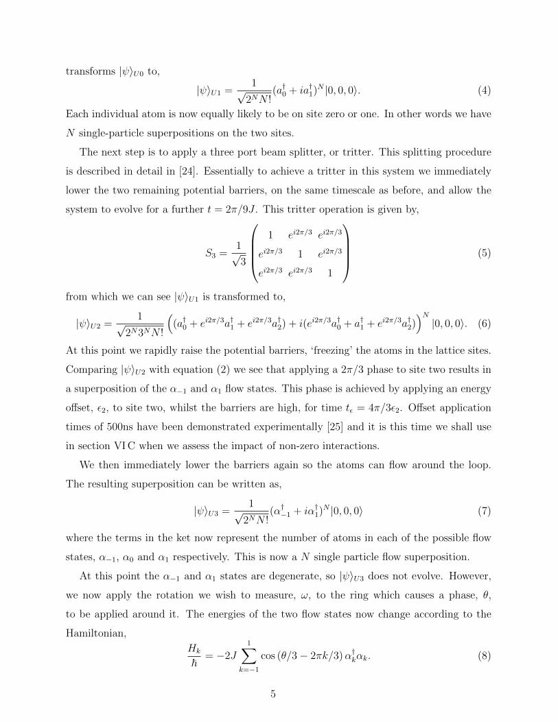
The next step is to apply a three port beam splitter, or tritter. This splitting procedure

is described in detail in [24]. Essentially to achieve a tritter in this system we immediately

lower the two remaining potential barriers, on the same timescale as before, and allow the

system to evolve for a further t = 2π/9J . This tritter operation is given by,

S3 =1√3

1 ei2π/3 ei2π/3

ei2π/3 1 ei2π/3

ei2π/3 ei2π/3 1

(5)

from which we can see |ψ〉U1 is transformed to,

|ψ〉U2 =1√

2N3NN !

((a†0 + ei2π/3a†1 + ei2π/3a†2) + i(ei2π/3a†0 + a†1 + ei2π/3a†2)

)N|0, 0, 0〉. (6)

At this point we rapidly raise the potential barriers, ‘freezing’ the atoms in the lattice sites.

Comparing |ψ〉U2 with equation (2) we see that applying a 2π/3 phase to site two results in

a superposition of the α−1 and α1 flow states. This phase is achieved by applying an energy

offset, ε2, to site two, whilst the barriers are high, for time tε = 4π/3ε2. Offset application

times of 500ns have been demonstrated experimentally [25] and it is this time we shall use

in section VI C when we assess the impact of non-zero interactions.

We then immediately lower the barriers again so the atoms can flow around the loop.

The resulting superposition can be written as,

|ψ〉U3 =1√

2NN !(α†−1 + iα†1)

N |0, 0, 0〉 (7)

where the terms in the ket now represent the number of atoms in each of the possible flow

states, α−1, α0 and α1 respectively. This is now a N single particle flow superposition.

At this point the α−1 and α1 states are degenerate, so |ψ〉U3 does not evolve. However,

we now apply the rotation we wish to measure, ω, to the ring which causes a phase, θ,

to be applied around it. The energies of the two flow states now change according to the

Hamiltonian,

Hk

~= −2J

1∑k=−1

cos (θ/3− 2πk/3)α†kαk. (8)

5

After a time tω, and ignoring global phases, the state has evolved to

|ψ〉U4 =1√

2NN !

(ei2Jtω cos(θ/3+2π/3)(α†−1) + iei2Jtω cos(θ/3−2π/3)(α1)

†)N|000〉 (9)

and so a phase difference of φ = 2√

3Jtω sin(θ/3) is established between the two flows.

We now wish to read-out this phase difference from which we can directly determine ω

since ω = hθ/(L2m) where m is the mass of the atom and L is the circumference of the

ring. The read-out procedure involves sequentially undoing all the operations performed

prior to the phase shift. This is analogous to standard Mach-Zehnder interferometry where

an (inverse) beam splitter is placed after the phase shift to undo the initial beam splitting

operation.

The undoing process begins with the application of a −2π/3 phase to site two giving,

|ψ〉U5 =1√

2N3NN !

((a†0 + ei2π/3a†1 + ei2π/3a†2) + ieiφ(ei2π/3a†0 + a†1 + ei2π/3a†2)

)N|0, 0, 0〉

(10)

where the terms in the kets now, once again, represent the number of atoms in sites zero,

one and two. Next we undo the tritter by applying an inverse tritter, S−13 = S†3. The inverse

tritter operation is discussed in detail in [24] but essentially is achieved by lowering all three

barriers and allowing the system to evolve for time t = 4π/9J (i.e. twice as long as for a

tritter) giving,

|ψ〉U6 =1√

2NN !

(a†0 + ieiφa†1

)N|0, 0, 0〉 (11)

which is equivalent to |ψ〉U1 but with a phase difference, φ.

Finally we apply an inverse two port 50:50 beam splitter. This is achieved in just the

same way as the two port beam splitting operation described above, but with a hold time

of t = 3π/4J rather than t = π/4J . The resulting state is,

|ψ〉U7 =1√N !

(cos

(φ

2

)(a†0)− sin

(φ

2

)(a†1)

)N|0, 0, 0〉 (12)

meaning the probabilities of detecting each atom at site zero and site one are,

P0 = cos2(φ

2

)(13)

P1 = sin2

(φ

2

).

Since the atoms are independent the total number detected in the two sites is given by a

binomial distribution. The mean number of atoms detected at site zero is therefore 〈n0〉 =

6

N cos2(φ/2) and at site one it is 〈n1〉 = N sin2(φ/2). By counting the number of atoms

detected at each site we can determine φ, and hence ω, just as in a typical Mach-Zehnder

interferometer.

The precision with which this scheme enables us to measure ω can be found by calculating

the quantum Fisher information, FQ. This is a tool for evaluating the precision limits of

quantum measurements and is independent of the measurement procedure. For a pure state

|Ψ(φ)〉 it is given by [26],

FQ = 4[〈Ψ′(φ)|Ψ′(φ)〉 − |〈Ψ′(φ)|Ψ(φ)〉|2

]. (14)

We convert this into an uncertainty in φ using the Cramer-Rao lower bound [27–29],

∆φ ≥ 1/√FQ. (15)

Using |ψ〉U4 we find the maximum resolution scaling of φ with N is N−1/2, or equivalently

∆θ ∼√

3/(2Jtω cos(θ/3)√N). This translates to an uncertainty in ω of,

∆ω ∼(

h

L2m

) √3

2Jtω√N

(16)

where we have made the approximation that θ/3 � 1. This has the well-known 1/√N

scaling that is a signature of the shot-noise limit.

To summarize, shot-noise limited measurements of rotations are made as follows:

1. Apply a two port 50:50 beam splitter to the first two modes of the state |N, 0, 0〉.

2. Perform a three port beam splitter (tritter) operation to the state.

3. Apply a 2π/3 phase to site two.

4. Leave the system to evolve for time tω under the rotation, ω.

5. Apply a −2π/3 phase to site two.

6. Perform an inverse tritter operation on the state.

7. Apply an inverse two port 50:50 beam splitter to the first two modes.

8. Count the number of atoms in each site.

We will now show how our scheme can be modified to create entangled states and will

investigate the effect of this entanglement on the precision scaling of our rotation measure-

ments.

7

IV. SCHEME 2: THE BAT STATE

We begin with N/2 atoms on site zero and on site one, i.e. |ψ〉B0 = |N/2, N/2, 0〉. The

production of dual Fock state BECs in a double well potential was first proposed in [30].

This number squeezed state could be achieved by slowly applying a double well trapping

potential to a condensate so that a phase transition occurs to the Mott insulator state and

has been demonstrated experimentally in three-dimensional optical lattices [31]. Initially

the barriers between the three sites are high and, as in scheme 1, a two port beam splitter

is applied to the first two modes of |ψ〉B0. The resulting output is sometimes referred to as

a ‘bat’ state since a plot of the amplitudes in the number basis resemble the ears of a bat.

Steps two to seven are identical to scheme 1 resulting in,

|ψ〉B4 =1√

2N(N/2)!

((α†−1)

2 + ei2φ(α†1)2)N/2

|0, 0, 0〉 (17)

and

|ψ〉B7 =1

2N (N/2)!

((a†0 − ia

†1

)2+ ei2φ

(−ia†0 + a†1

)2)N/2|0, 0, 0〉 (18)

where a global phase has been ignored and φ is again given by φ = 2√

3Jtω sin(θ/3). This is

very similar to the scheme in [16], where a bat state is used to measure a phase difference in

a general Mach-Zehnder interferometer set-up, and in fact results in the same output. The

difference between the schemes is that ours has been adapted to measure a rotation around

a ring of lattice sites rather than a general phase between two paths.

To determine φ we could count the number of atoms detected at each site and repeat.

However, this requires nearly perfect detector efficiencies [32] and so is experimentally chal-

lenging. Instead we use the read-out scheme described (in detail) in [16] to make our

measurements.

Essentially, after step seven the system is then left to evolve with the barriers high for τ =

π/16V (note in the original paper τ = π/8U because U = 2V here). The trapping potentials

are then switched off and after some expansion time interference fringes are recorded. These

two steps are the read-out steps and are what we shall refer to as step eight. The scheme is

repeated many times and the visibility, V , of the fringes is calculated as in [16]. From these

visibility measurements we determine φ directly. Note that the quantum Fisher information

depends only on the final state of the system and not on the measurement procedure.

8

As such we use |ψ〉B4 to determine the precision scaling of θ with N and find ∆θ ∼√

3/(2Jtω cos(θ/3)√N(N/2 + 1)). This means the uncertainty in ω is,

∆ω ∼(

h

L2m

) √3

2Jtω cos(θ/3)√N(N/2 + 1)

∼(

h

L2m

) √3√

2JtωN, (19)

where we have made the approximations N � 1 and θ/3 � 1. This has the same number

scaling as the Heisenberg limit.

We now present a third scheme which offers a slight improvement in the precision scaling

of our measurements. We then consider the advantages and disadvantages of schemes 2 and

3 and discuss their experimental limitations.

V. SCHEME 3: THE NOON STATE

This scheme is very similar to scheme 1, the only difference is that the two port 50:50

beam splitter (and its inverse) is replaced with a two port quantum beam splitter (and

an inverse two port quantum beam splitter). A two port quantum beam splitter (QBS) is

defined as a device [33] that outputs (|N, 0〉 + eiξ|0, N〉)/√

2 when |N, 0〉 is inputted. The

terms in the kets represent the number of particles in the two modes. This output is called

a NOON state.

As in scheme 1, the three potential barriers are initially high and N atoms are inputted

into site zero, |ψ〉N0 = |N, 0, 0〉. The first step is to apply the QBS. This is done using a

scheme proposed in [15].

The QBS begins with the application of a two port 50:50 beam splitter between sites

zero and one, as previously described. A π/2 phase is then applied to one of the two sites

using an energy offset as above. At this stage V � J and the interactions are tuned such

that their strength on one site is an integer multiple of the strength on the second site [46].

The system is left to evolve for t = π/2V in this regime after which a second two port beam

splitter is applied. These steps output,

|ψ〉N1 →1√2N !

((a†0)

N + eiξ(a†1)N)|0, 0, 0〉. (20)

where ξ is some relative phase established by the splitting procedure.

Here we have a superposition of all N atoms on site zero and all on site one. At the

equivalent stage in scheme 1 we had N single particle superpositions (see equation 4). It is

this difference that is responsible for the improved precision.

9

Steps two to six are identical to those in scheme 1 giving,

|ψ〉N4 =1√2N !

((α†−1)

N + eiξeiNφ(α†1)N)|0, 0, 0〉. (21)

and

|ψ〉N6 =1√2N !

((a†0)

N + eiξeiNφ(a†1)N)|0, 0, 0〉. (22)

Finally we apply an inverse two port quantum beam splitter to the system. This is

achieved by sequentially undoing all the steps of the QBS. So,

1. Apply an inverse two port beam splitter.

2. Raise the barriers and tune the interactions as before.

3. Leave the system to evolve for t = π/2V .

4. Apply a −π/2 phase to the same site as before.

5. Apply a second inverse two port beam splitter.

6. Raise the barriers.

This results in all N atoms detected at site zero or all at site one with respective proba-

bilities,

P0 = cos2(Nφ

2

)(23)

P1 = sin2

(Nφ

2

).

By repeating the scheme many times, each time recording the site on which all N

atoms are detected, φ, and hence ω, can be determined. Using the quantum Fisher

information and the Cramer-Rao lower bound the maximum resolution of scheme 3 is

∆θ ∼√

3/(2Jtω cos(θ/3)N) meaning, for θ/3� 1,

∆ω ∼(

h

L2m

) √3

2JtωN. (24)

We see the NOON state offers a slight improvement in resolution scaling over scheme 2.

It has the same number scaling, but the numerical factor is√

2 better. However, this slight

improvement in resolution may come at great experimental expense. We now investigate

the effect of experimental limitations on schemes 2 and 3.

VI. COMPARISONS AND PRACTICAL LIMITATIONS

Both schemes 2 and 3 allow Heisenberg limited precision measurements of small rotations

with the precision capabilities of scheme 3 being marginally favorable. Our descriptions

10

thus far, however, have only considered the idealized case and we have neglected important

physical processes that may limit the experimental feasibility of the schemes. We now

reevaluate the schemes when these limitations are accounted for.

A. Particle loss

We need to account for the fact that atoms may be lost during the schemes. It is well

known that NOON states undergoing particle loss decohere quickly and so soon lose their

Heisenberg limited sensitivity. However, it has previously been shown that certain entangled

Fock states, that allow sub-shot noise phase measurements, are much more robust to these

losses [34]. Here we wish to see how resistant the bat state is to particle loss in comparison

to the NOON state by determining the precisions afforded by both schemes in the presence

of loss.

We investigate the effects of loss using a procedure described in [35, 36] which models

loss from the middle section (between the two beam splitters) of an ordinary two path

interferometer using fictitious beam splitters whose transmissivities, η, are directly related

to the rate of loss. The equivalent loss in our schemes is loss from the momentum modes

during tω. It was shown in [35, 36] that the time at which loss occurs during this interval is

irrelevant. Since losses are equally likely from both modes we consider equal loss rates, η,

from each momentum mode.

To compare the effects of particle loss on our two schemes we determine FQ and ∆φ for

each scheme for different loss rates, or different η. As shown in [35, 36] FQ varies with η as,

FQ =N∑l=0

FQ

l∑lα1=0

plα1 ,l−lα1 |ξlα1 ,l−lα1 (φ)〉〈ξlα1 ,l−lα1 (φ)|

(25)

where l is the total number of atoms lost, lα1 is the number lost from the α1 mode, plα1 ,l−lα1

is the probability of each loss event and

|ξlα1 ,l−lα1 (φ)〉 =1

√plα1 ,l−lα1

N−(l−lα1 )∑m=lα1

βmeimφ√Bmlα1 ,l−lα1

|m− lα1 , N −m− (l − lα1)〉. (26)

Here

Bmlα1 ,l−lα1

=

(m

lα1

)(N −ml − lα1

)ηN(η−1 − 1)l (27)

11

and βm is

βm =iN/2√m!√

(N −m)!

2N/2(m/2)!(N/2−m/2)!× 1 + (−1)m

2(28)

for the bat state and

βm =

1/√

2 for m = 0, N

0 for m 6= 0, N

for the NOON state. FQ is found numerically using

FQ = Tr[ρ(φ)A2] (29)

where A is the symmetric logarithmic derivative which is defined by,

∂ρ(φ)

∂φ=

1

2[Aρ(φ) + ρ(φ)A]. (30)

It is given by,

(A)ij =2

λi + λj

[∂ρ(φ)

∂φ

]ij

(31)

in the eigenbasis of ρ(φ), where λi,j are the eigenvalues of ρ(φ). Combining these equations

gives [37],

FQ =∑i,j

2

λi + λj

∣∣∣∣⟨Ψi

∣∣∣∣∂ρ(φ)

∂φ

∣∣∣∣Ψj

⟩∣∣∣∣2 (32)

where Ψi,j are the eigenvectors of ρ(φ).

Figure 1 shows how ∆φ varies with η for the two schemes when N = 10. As expected the

NOON state achieves the best precision when η = 1, or when there are no losses. However,

as η decreases the bat state soon becomes the favored scheme. The lower bound of the

shaded area is the Heisenberg limit and the upper bound is the precision achievable when an

uncorrelated, or classical, input state is used, as in scheme 1. We see the uncorrelated state

soon outperforms the NOON state. However, the bat state outperforms the uncorrelated

input for approximately half the loss rates shown. Since it is unlikely half the atoms would

be lost in an experiment, the bat state, unlike the NOON state, appears to offer an experi-

mentally feasible increase in precision over classical precision measurement experiments. In

the remainder of the paper we therefore assess the impact of experimental limitations on

just scheme 2.

12

!

"#

0 0.2 0.4 0.6 0.8 10

0.2

0.4

0.6

0.8

1

FIG. 1: The uncertainty of φ for different rates of loss, η, for N = 10. The blue dashed line shows

∆φ for scheme 2 and the green solid line shows ∆φ for scheme 3. The upper bound of the shaded

region is the precision afforded by scheme 1 (the classical precision limit - black dashed-dotted

line) and the lower bound shows the Heisenberg limit. Scheme 3 soon becomes less favorable than

scheme 1, whilst scheme 2 is much more robust to losses.

B. Variations in N between experimental runs

Our scheme requires many repetitions of the gyroscope procedure in order to build up

interference fringes from which φ can be determined. We have assumed thus far that each

run involves exactly N atoms. However, in an experiment N is likely to fluctuate between

runs. The effect of fluctuations of order√N on the bat state input are discussed in [16].

In that case, an ordinary two-path linear interferometer is used but the same results apply

here. It is shown that while the interference fringe signal is degraded by these fluctuations,

the approximate Heisenberg limited sensitivity of the scheme is not destroyed. As expected,

the larger N , the smaller the fluctuation effects, which is good since we would ideally work

in the limit of large N since this gives the best improvement in precision.

C. Interactions

So far we have considered only the idealized system setting V = 0 (apart from in the

detection step, step eight, where we require large interactions to minimize small coupling

13

effects), and J = 0 in the low coupling regime. While interactions can be tuned to extremely

small values using Feshbach resonances it is an unrealistic assumption to discount them

altogether. Likewise it is unrealistic to completely neglect coupling effects in the low coupling

regime. Here we consider the effect of non-zero interactions and non-zero coupling strengths

in the low coupling regime on scheme 2. To determine experimental orders of magnitude for

V and J we use the approximations [38],

V ≈ 2asV340 E

14R

~(√λD)

(33)

J ≈ ER2~

exp

(−(π2

4

)√V0ER

)√ V0ER

+

(√V0ER

)3 (34)

where as is the scattering length, V0 the barrier height, ER the recoil energy, λ the wavelength

of the lattice light and D the transverse width of the lattice sites. Feshbach resonances

can tune as to values smaller than the Bohr radius for some BECs [39] and in the high

coupling regime barrier heights of order V0 = 2ER have been demonstrated [40]. Using

light of wavelength λ = D = 10µm and 87Rb atoms, interactions can therefore be tuned

to V ∼ 10−3Hz and J ∼ 10Hz in this regime. While in the low coupling regime, where

V0 = 35ER [23], we find V ∼ 10−2Hz and J ∼ 10−2Hz. Note that in the detection process

the system evolves for t = π/16V with high potential barriers. Here we require large

interactions to minimize small coupling effects. Taking as = 9000a0 [41] gives V ∼ 100Hz.

Using these values we assess the impact of non-zero interactions and coupling strengths.

As N increases the occupation number per site increases and as such the effect of non-zero

interactions become more pronounced. We would therefore like to determine the maximum

number of atoms our system can tolerate before these effects become too destructive. To

do this we measure the fidelity between the output of the gyroscope in the idealized case

in which V = 0 (except in step eight) and J = 0 in the low coupling regime with the same

output when V ∼ 10−3 in the high coupling regime, V ∼ 10−2 in the low coupling regime and

J ∼ 10−2 in the low coupling regime. The maximum N that can be tolerated is taken to be

the first N for which this fidelity falls below 0.99. In this simulation we have taken tω = 1s

and θ = π/100. Figure 2 shows how the fidelities decrease as N increases. We see that by

our definition the maximum number of atoms the system can tolerate is approximately 60.

Squeezed states with larger numbers of atoms have been demonstrated experimentally [10]

and as such interactions are likely to be one of the main limiting factors of this scheme.

14

0 10 20 30 40 50 60 700.96

0.97

0.98

0.99

1

N

Fidelity

FIG. 2: The fidelity between the output of scheme 2 in the idealized case (where V = 0, and J = 0

in the low coupling regime) with the output in the non-idealized case (where V ∼ 10−3 in the high

coupling regime, V ∼ 10−2 in the low coupling regime and J ∼ 10−2 in the low coupling regime)

for different numbers of input atoms. Here θ = π/100 and tω = 1s.

D. Metastability

Our gyroscope scheme relies on the two counterpropagating superfuid states being stable

at least over the timescale of the measurement that we want to make. There has been a

lot of discussion and analysis of what conditions need to be met so that a superfluid cur-

rent persists (or is metastable) in BECs. In a toroidal trap, for example, the condition

for metastability is that the mean interaction energy per particle is greater than the single

particle quantization energy h2/mL2 [42]. This can be shown to be equivalent to the condi-

tion that the superfluid velocity is less than the velocity of sound, which is just the Landau

criterion for the metastability of superfluid flow. Persistent superfluid flows have recently

been experimentally observed for BECs in toroidal traps [43].

There has also been an analysis of the metastability requirements for a system that is

directly relevant to our scheme, i.e. a superfluid Bose gas trapped in a ring optical lattice

[44]. In this work, it was shown that any disorder due to energy offsets, ε, on the lattice

sites in the ring can cause dissipation by providing a coupling pathway between states

with opposite quasi-momentum. If, however, there are interactions between the atoms, the

energy levels are shifted and this mismatch means that the different supercurrent states

15

become effectively decoupled and so the supercurrent should persist. Kolovsky showed that

for states with low values of quasimomentum (such as the ±1 unit of angular momentum

states that we consider) the minimum strength of the interactions must be Vmin ≈ 8ε/N .

Taking parameters from our scheme, in the strong tunneling region, we have J ∼ 10Hz and

V ∼ 10−3Hz. This means that we require ε < NV/8 ≈ 10−2Hz, for N ≈ 60. By stabilizing

the energy offsets to this level (or increasing the interactions) persistent supercurrents should

be able to be achieved.

E. Comparison with other schemes

At this point we note that our precision analysis is for the case of a single shot, i.e. N

atoms are loaded into the lattice and a single measurement is made over time tω correspond-

ing to a particle flux of N/tω. In reality, the results of many runs will be combined to give

a measurement of the rotation. Suppose we repeat the measurement n times to give a total

integration time of τ = ntω[47]. In this case, we get

∆ω ≈(

h

L2m

) √3√

2nJtωN=

(h

L2m

) √3√

2tωτJN=

S√τ, (35)

where the short-time sensitivity is given by,

S =

(h

L2m

) √3√

2tωJN. (36)

Substituting in approximate values for our setup in the strong coupling regime (i.e. J ≈

10Hz, N ≈ 60, tω ≈ 1s and L = 2π × 20µm [22]), we get S ≈ 10−3 rads−1/√

Hz. This

compares unfavorably with other atom interferometry schemes which can achieve sensitivities

better than 10−8 rads−1/√

Hz [45]. These other schemes achieve improved sensitivities by

having much larger particle fluxes (e.g. 6× 108 atoms/s) and much larger areas enclosed by

their interferometer paths (e.g. 22 mm2) [45].

The scheme presented here is therefore unlikely to challenge the overall precision offered

by other techniques, except perhaps in specialised cases where the number of atoms available

is restricted to a small number or the area of the interferometer must be very small. The

main interest of this scheme, however, is that it proposes a means of creating macroscopic

superpositions of persistent superfluid flows and that these could show evidence of Heisenberg

scaling of measurement precision. This in itself would be of fundamental interest. In order

16

to improve its short-term sensitivity, however, it is likely to be difficult to create entangled

states with very large numbers of particles, so a different configuration would need to be

used to greatly enhance the enclosed area of the interferometer.

Alternatively nonlinear couplings of the atoms and the rotation could potentially be used

to achieve precision scalings of N−3/2 using unentangled atoms [19, 20]. The reliance of

such a scheme on unentangled atoms would allow for much larger atom numbers than in

our scheme and as such seems to offer a possible way of improving upon current gyroscope

precisions. However, the challenge of this scheme would be coupling the angular momentum

and the atomic scattering lengths.

VII. CONCLUSION

We have presented three schemes to measure small rotations applied to a ring of lattice

sites by creating superpositions of ultra-cold atoms flowing in opposite directions around

the ring. Two of these schemes are capable of Heisenberg limited precision measurements

where the precision scales as 1/N . The two schemes use different entangled states. While

the scheme that used a NOON state gave slightly better precision in the idealized case, after

consideration of experimental limitations it was shown that the bat state is likely to be the

preferred candidate largely due to its robustness to particle loss. Importantly the bat state

outperformed the case of unentangled particles for modest loss rates. The effects of non-zero

interactions were shown to limit the preferred scheme to approximately 60 atoms and as such

this scheme is not capable of outperforming the precision of existing atomic gyroscopes at

present. However, the interesting result is the Heisenberg scaling of the precision. All the

steps in this scheme should be within reach of current technologies which is promising for

its experimental implementation.

This work was supported by the United Kingdom EPSRC through an Advanced Re-

search Fellowship GR/S99297/01, an RCUK Fellowship, and the EuroQUASAR programme

EP/G028427/1.

[1] G. Sagnac, C. R. Acad. Sci. 157, 708 (1913).

[2] B. Yurke, Phys. Rev. Lett. 56, 1515 (1986).

17

[3] C. M. Caves, Phys. Rev. D 23, 1693 (1981).

[4] H. Lee, P. Kok and J. P. Dowling, J. Mod. Opt. 49, 2325 (2002).

[5] V. Giovannetti, S. Lloyd and L. Maccone, Science 306, 1330 (2002).

[6] J. P. Dowling, Phys. Rev. A 57, 4736 (1998).

[7] C. Orzel, A. K. Tuchman, M. L. Fenselau, M. Yasuda and M. A. Kasevich, Science 291, 2386

(2001).

[8] W. Li, A. K. Tuchman, H. Chien and M. A. Kasevich, Phys. Rev. Lett. 98, 040402 (2007).

[9] S. A. Haine and M. T. Johnsson, Phys. Rev. A 80, 023611 (2009).

[10] J. Esteve, C. Gross, A. Weller, S. Giovanazzi and M. K. Oberthaler, Nature 455, 1216 (2008).

[11] L. Pezze, L. A. Collins, A. Smerzi, G. P. Berman and A. R. Bishop, Phys. Rev. A 72, 043612

(2005).

[12] L. Pezze, A. Smerzi, G. P. Berman, A. R. Bishop and L. A. Collins, Phys. Rev. A 74, 033610

(2006).

[13] L. Pezze and A. Smerzi, Phys. Rev. Lett. 102, 100401 (2009).

[14] P. Bouyer and M. A. Kasevich, Phys. Rev. A 56, R1083 (1997).

[15] J. A. Dunningham and K. Burnett, J. Mod. Opt. 48:12 1837 (2001).

[16] J. A. Dunningham and K. Burnett, Phys. Rev. A, 70, 033601 (2004).

[17] L. Pezze and A. Smerzi, Europhys. Lett. 78, 30004 (2007).

[18] C. P. Search, J. R. E. Toland and M. Zivkovic, Phys. Rev. A 79, 053607 (2009).

[19] S. Boixo et al., Phys. Rev. Lett. 101, 040403 (2008).

[20] S. Boixo et al., Phys. Rev. A, 80, 032103 (2009).

[21] V. Boyer et al., Phys. Rev. A 73 031402 (2006).

[22] K. Henderson, C. Ryu, C. MacCormick and M. G. Boshier, New J. Phys. 11, 043030 (2009).

[23] M. Greiner, O. Mandel, T. W. Hansch and I. Bloch, Nature, 419, 51 (2002).

[24] J. J. Cooper, D. W. Hallwood and J. A. Dunningham, J. Phys. B 42, 105301 (2009).

[25] J Denschlag et al., Science 287, 97 (2000).

[26] S. L. Braunstein, C. M. Caves and G. J. Milburn, Ann. Phys. (N.Y.) 247, 135 (1996).

[27] C. Rao, Bull. Calcutta Math. Soc. 37, 81 (1945).

[28] H. Cramer, Mathematical Methods of Statistics, Princeton Univ. Press, Princeton, NJ (1946).

[29] C. W. Helstrom, Quantum Detection and Estimation Theory, Academic Press, New York

(1976).

18

[30] R. W. Spekkens and J. E. Sipe, Phys. Rev. A 59, 3868 (1999).

[31] M. Greiner et al., Nature (London) 415, 39 (2002).

[32] T. Kim, Y. Ha, J. Shin, H. Kim and G. Park, Phys. Rev. A 60, 708 (1999).

[33] J. Dunningham and T. Kim, J. Mod. Opt. 53:4, 557 (2006).

[34] S. D. Huver, C. F. Wildfeuer and J. P. Dowling, Phys. Rev. A 78, 063828 (2008).

[35] R. Demkowicz-Dobrzanski et al., Phys. Rev. A 80, 013825 (2009).

[36] U. Dorner et al., Phys. Rev. Lett. 102, 040403 (2009).

[37] C. Ping and L. Shunlong, Front. Math. China 2, 359 (2007).

[38] S. Scheel, J. Pachos, E. A. Hinds and P. L. Knight, Lect. Notes Phys. 689, 47 (2006).

[39] C. Chin, R. Grimm, P. Julienne and E. Tiesinga, arXiv:0812.1496v1 (2008).

[40] M. Jona-Lasinio et al., Phys. Rev. Lett. 91, 23 (2003).

[41] S. L. Cornish, N. R. Claussen, J. L. Roberts, E. A. Cornell and C. E. Wieman, Phys. Rev.

Lett. 85, 1795 (2000).

[42] A.J. Leggett, Rev. Mod. Phys. 73, 307 (2001).

[43] K. Helmerson et al., Nuclear Physics A 790, 705 (2007); C. Ryu et al., Phys. Rev. Lett. 99,

260401 (2007).

[44] Andrey R. Kolovsky, New J. Phys. 8, 197 (2006).

[45] T. L. Gustavson, P. Bouyer and M. A. Kasevich, Phys. Rev. Lett. 78, 2046 (1997).

[46] This ensures that the required superposition is created independent of the total number of

atoms, N

[47] Note that there are still N atoms on each run, which lasts for time tω, so the particle flux is

the same as for the case of a single run.

19