1

Atomic retrodiction

Stephen M. Barnett1, David T. Pegg2, John Jeffers1 and Ottavia

Jedrkiewicz3

1Department of Physics and Applied Physics, University of Strathclyde, Glasgow G4

0NG, U.K.

2School of Science, Griffith University, Nathan, Brisbane 4111, Queensland, Australia.

3Department of Physics, University of Essex, Wivenhoe Park, Colchester CO4 3SQ,

U.K.

Abstract. Measurement of a quantum system provides information

concerning the state in which it was prepared. In this paper we show how

the retrodictive formalism can be used to evaluate the probability

associated with any one of a given set of preparation events. We illustrate

our method by calculating the retrodictive density operator for a two-level

atom coupled to the electromagnetic field.

2

1. Introduction

Quantum theory is primarily about prediction, that is calculating the probabilities

associated with any future measurement outcomes given information about the

preparation, the subsequent evolution of the system and the measurement device to be

used. A simple example is the probability that an initially excited atom, prepared at

preparation time tp, will be found by a suitable detector in its ground state at some

measurement time tm . This problem can be solved straightforwardly in the usual

formalism, which we shall refer to in this paper as the predictive formalism. In this

formalism, we speak of preparing the system in some state that depends only on the

outcome of the preparation event. This state is most generally represented by a density

operator that subsequently changes with time. Associated with the measuring device

is, in general terms, a probability operator measure (POM) (Helstrom 1976).

Projection of the density matrix at the time of measurement onto an element of the

POM determines the probability of the outcome associated with that element. Ideal

von Neumann measurements of an observable have possible measurement outcomes

given by its eigenvalues and the associated POM element is simply the projector onto

the corresponding eigenvector. In this formalism the state represents our knowledge

of the preparation event.

Sometimes, for example in communication situations, we only have

knowledge of the outcome of a measurement event and wish to deduce from this

3

information about the preparation event. It is possible to use Bayes’ theorem (Box and

Tiao 1973) together with the predictive formalism for this purpose, but it is more

direct to use the less common retrodictive formalism of quantum mechanics

(Aharonov et al 1964, Penfield 1966, Belinfante 1975, Pegg and Barnett 1999,

Barnett et al 2000a,b). In this formalism a state is assigned solely on the basis of the

outcome of the measurement. We will refer to such a state as a retrodictive state.

Thus instead of speaking of preparing the system in a state, we speak of measuring the

system to be in a state. The retrodictive state transforms as we go back in time to the

preparation event, at which time projection onto an operator associated with the

preparation device determines the probability that the system was prepared in the state

associated with that operator.

In previous work we have used the retrodictive formalism to study some

problems in quantum optics including photon antibunching and EPR correlated

photons, optical state preparation and quantum communications (Pegg and Barnett

1999, Barnett and Pegg 1999, Barnett et al 2000a,b). In this paper we shall exploit the

formalism to study some preparation probabilities in a two-level atom interacting with

an electromagnetic field.

2. Retrodiction

2.1. Closed systems

We refer to a quantum mechanical system as closed if the system is prepared, evolves

4

unitarily without interaction with another system and is then measured. A simple

example involves a spin-half particle which can be prepared in an "up" or "down"

state with a Stern-Gerlach apparatus. Another such apparatus can give a measurement

result that the atom is in either of the states ± corresponding, respectively, to the

angles θ and π θ+ to the up axis with no change of state between preparation and

measurement. In one experiment we may know the outcome of the preparation event

was the up state. We can then use the usual predictive formalism of quantum

mechanics to calculate the probability that the outcome of the measurement

corresponds to the state + . The result is up + 2, that is, cos /2 2θ .

In a second experiment we may be told that the outcome of the measurement

corresponded to the state + but have no knowledge of the preparation event other

than that the up and down states had equal a priori probabilities of being prepared.

We wish to calculate, on the basis of this knowledge, the a posteriori probability that

the atom was prepared in the down state. For this we would use the retrodictive

formalism and assign the system the retrodictive state + just prior to the

measurement. Knowing that the state does not change between preparation and

measurement we would assign the retrodictive state + to the atom just after the

preparation event. The probability that the atom was prepared in the down state is

then + down2, that is sin /2 2θ . It is customary to speak of the event associated

with the projection as the collapse of the wavefunction. In the predictive formalism,

this takes place at the time of the measurement but in the retrodictive formalism it

coincides with the preparation event.

5

We can treat the above simple example more formally in terms of a

probability operator measure. The essential features of a POM are reviewed in

Appendix A. For the case above, the measurement POM has two elements, + +

and − − each associated with a possible measurement outcome and which sum to

the unit operator. The retrodictive density operator associated with a particular

outcome is just the corresponding POM element, normalised if necessary to have unit

trace (Barnett et al 2000a). The retrodictive density operator associated with the

outcome corresponding to detection of state + at the time of measurement is

therefore simply + + . As there is no evolution in this case between measurement

and preparation, this is also the retrodictive density operator ˆ ( )ρθretr

pt at the

preparation time tp. The source is unbiased because the up and down states have

equal probability of being produced. The preparation POM elements (see appendix A

and Barnett et al 2000a) Ξp are thus up up and down down. The probability

P( | )up + that the atom was prepared in the up state if detected in the state + is

Tr retrp up

ˆ ( ) ˆρθ t Ξ[ ].

Suppose we change the example slightly so that the preparation apparatus

includes some type of filter, say, which reduces the a priori probability P( )down for

the down state to below one-half. Then instead of describing the (now biased)

preparation device by POM elements Ξp we use instead the operators Λ p. These can

be summed to form the a priori preparation density operator:

6

ˆ ˆΛ Λ= ∑p

p . (2.1)

In general the terms Λ p can be associated with mixed states, but in our example here

there are two terms, ˆ ( )Λup up up up= P and Λdown = P( )down down down. In the

absence of any further information as to what state was actually prepared, the best

description we could give of the prepared state of the atom in the predictive formalism

would be to assign it the predictive density operator ˆ ˆΛ Λup down+ based on our a priori

knowledge. If we do know which state was actually prepared, say the up state, then

we would assign the predictive density operator ˆ / ˆΛ Λup upTr( ) . If, on the other hand,

we do not know which state was actually prepared but know that the atom is detected

in the state + we can calculate retrodictively the probability that the atom was

prepared in the up state by projecting the retrodictive density operator corresponding

to this measurement outcome onto the appropriate term Λ p and obtain, after

normalisation,

Pt

t pp

( | )ˆ ( ) ˆ

ˆ ( ) ˆup

Tr

Tr

retrp up

retrp

+ =[ ]

[ ]∑ρ

ρθ

θ

Λ

Λ (2.2)

7

A corresponding expression holds for the probability that the atom was prepared in

the down state if detected in the state + .

We can summarise the predictive and retrodictive quantum formalisms for

closed systems as follows. In the predictive formalism Λ p, associated with outcome

p of the preparation device, becomes upon normalisation the predictive density

operator. This operator evolves forward in time until it is projected onto Πm to

determine the probability of measurement outcome m. In the retrodictive formalism

Πm , associated with outcome m of the measuring device, becomes upon

normalisation the retrodictive density operator. This operator evolves backwards in

time until it is projected onto Λ p to determine the probability of preparation outcome

p.

2.2. Open systems

An open system is one in which the subsystem S under study interacts with another

subsystem. Often this second subsystem is larger and is referred to as the environment

E. Normally we have at least some statistical information about the initial state of the

environment and can assign it a density matrix. In the predictive formalism we can

calculate the probability of obtaining a particular result of a measurement by finding

the unitarily-evolved predictive density-operator for the combined system at the time

8

of measurement and projecting this onto the appropriate combined POM element. In

the usual case, in which we do not make any measurement of the environment, we can

write the combined measurement POM element as proportional to the product of the

POM element Πm associated with the outcome m for S and the unit operator 1E on the

space of the environment states. An alternative predictive approach is to represent the

subsystem S by a reduced density operator at the time of preparation, which is the

trace of the density operator of the complete system over the states of the

environment. The subsequent non-unitary evolution of the reduced density matrix is

determined by a master equation. This equation is constructed so as to produce the

correct measurement probability when the evolved reduced density operator at the

time of the measurement is projected onto Πm . Thus, although the complete system

usually evolves into an entangled state we can, in the usual predictive formalism,

represent the state of S in the limited sense that from it we can calculate the

probability for S to be detected in any particular state, conditioned on no information

being obtained about the state of the environment.

In the retrodictive formalism of quantum mechanics, the retrodictive density

operator of the system being measured is, immediately prior to the measurement,

simply the POM element associated with the measurement outcome with a suitable

normalisation factor (Barnett et al 2000a). Thus if the measurement gives an outcome

m for S but no information about the environment, we can find the retrodictive density

9

operator at an earlier time tp as

ˆ ( )ˆ ˆ ˆ ˆ

ˆ ˆ

†

ρ retrp

E

ES ETrt

U Um

m

= [ ]1

1

ΠΠ

(2.3)

where U is the forward time shift operator from the time tp to time tm , the time of the

measurement.

The terms Λ p of the preparation device density operator for the system

comprising S and E can be written as ˆ, ,Λ Λp pS E. If the preparation device is set up

such that in the predictive formalism the environment always has the same initial state

ˆ ( )ρEpred

pt , then ˆ ˆ ˆ ( ),Λ Λp p t= S Epred

pρ . The probability that the system was prepared at

time tp in the state corresponding to ˆ,Λ p S is thus given by

TrTr

TrES

retrp

ES E S Epred

p

ES S Epred

p

ˆ ( ) ˆˆ ˆ ˆ ˆ ˆ ˆ ( )

ˆ ˆ ˆ ˆ ˆ ( )

†,

†,

ρρ

ρt

U U t

U U tp

m p

m pp

ΛΠ Λ

Π Λ[ ] =

[ ][ ]∑1

=[ ]

[ ]∑Tr

Tr

S Sretr

S

S Sretr

S

ˆ ˆ

ˆ ˆ,

,

ρ

ρ

Λ

Λp

pp

(2.4)

where

ˆˆ ( ) ˆ ˆ ˆ

[ ˆ ( ) ˆ ˆ ˆ ]

†

†ρ

ρ

ρSretr E E

predp

ES Epred

p

Tr

Tr=

[ ]t U U

t U U

m

m

Π

Π. (2.5)

10

The reduced retrodictive density operator ρSretr is of course not the same as the

reduced predictive density operator. Nevertheless it is “reduced” in the sense that it

acts only on the state space of S and not on the environment states. As with the

reduced predictive density operator, this operator can be used to calculate only

probabilities conditioned on the measurement not providing any information about the

environment.

The main aim of this paper is to calculate ρSretr, which we shall refer to simply

as the retrodictive density operator, for some open atomic systems. We can obtain

the retrodictive density matrix elements in terms of a complete orthonormal basis set

of states i of S. We have from (2.5)

i kN

i t U U kmˆ ˆ ( ) ˆ ˆ ˆ†ρ ρS

retrE E

predpTr= [ ]1 Π

= [ ]1N

U k i t UmTrES Epred

pˆ ˆ ˆ ( ) ˆ †Π ρ (2.6)

where we have used the cyclic property of the trace and N is the denominator in (2.5).

By introducing a general time-independent operator in the form

ˆ,

A A i kS iki k

= ∑ , (2.7)

11

we can rewrite the retrodictive density matrix elements (2.6) as

i kN A

UA t Uki

mˆ [ ˆ ˆ ˆ ˆ ( ) ˆ ]†ρ ∂

∂ρS

retrES S E

predpTr= 1 Π . (2.8)

If AS has the form of an initial density matrix then we can find

TrES S Epred

p[ ˆ ˆ ˆ ˆ ( ) ˆ ]†ΠmUA t Uρ from the appropriate master equation. We can most easily

find the normalisation constant N by noting that

i iN A

UA t Ui ii

mi

∑ ∑= =ˆ [ ˆ ˆ ˆ ˆ ( ) ˆ ]†ρ ∂∂

ρSretr

ES S Epred

pTr1

1Π . (2.9)

Expression (2.8) is useful for obtaining the retrodictive density matrix elements

directly without first calculating preparation probabilities from (2.4). The retrodictive

density matrix can then be used to calculate the preparation probability for any state

by projection onto the associated preparation POM element Ξp or preparation density

operator term Λ p as appropriate.

An alternative approach, if we wish to calculate the preparation probability

associated with a particular preparation POM element Ξp without explicitly finding

the retrodictive density operator, is as follows. This probability is given by

12

Tr TrS Sretr

ES Epred

pˆ ˆ ˆ ( ) ˆ ˆ ˆ ˆ†ρ ρΞ Π Ξp m pN

t U U( ) = [ ]1. (2.10)

We can rewrite this using the cyclic property of the trace as

Tr TrS Sretr

S mˆ ˆ ˆ ˆ ( )ρ Ξ Π Ξp m pN

t( ) = [ ]1, (2.11)

where

ˆ ( ) ˆ ˆ ( ) ˆ ( ) ˆ †Ξ Ξp pt U t t Um E p Epred

pTr= [ ]ρ . (2.12)

If Ξp has the form of an initial density matrix we see from (2.12) that ˆ ( )Ξp tm has the

form of a reduced density matrix in the predictive formalism obtainable from the

appropriate master equation for the initial state of the environment (Barnett and

Radmore 1997). It is straightforward to generalise this approach for a preparation

density operator term Λ p in place of Ξp .

In general, finding the retrodictive density operator is more useful in that it

allows the subsequent calculation of the preparation probability of any state and this is

the approach we use for most of this paper. We do, however, illustrate the alternative

approach of the above paragraph by finding directly the preparation state probabilities

for a spontaneously emitting atom. For completeness, we also outline in Appendix B

13

another method devised specifically for calculating the retrodictive density operator

for a two-level atom.

3. Two-level atomic retrodiction

The retrodictive formalism for open systems allows us to calculate, from the outcome

of a measurement, the probability associated with an earlier preparation event. In the

preceding section we have presented formulae for obtaining directly either the

probabilities for particular state preparations, or the retrodictive density matrix

elements in any basis, which can then be used to calculate preparation probabilities.

Here we shall illustrate our methods by using some examples from atomic physics, all

based on the two-level atom coupled to the electromagnetic field. We work

throughout in an interaction picture in which the energies of the two atomic levels do

not appear in the Hamiltonian.

3.1. Spontaneously emitting atom

Consider first the simplest of open systems, the damped undriven two-level atom with

excited and ground states e and g . We assume that a measurement has been made

14

at time tm and that we know the state corresponding to the measurement result. We

wish to retrodict a preparation event that has taken place at an earlier time t tp m= − τ .

Equation (2.11) gives the probability that the atom was prepared in a state

corresponding to a particular preparation POM element. We simply need the

appropriate measurement POM element and the precise form of ˆ ( )Ξp tm . To be

specific, suppose we find the atom to be in the ground state, so that Πm = g g is our

measurement POM element. We seek, respectively, the probabilities that the atom

was prepared in the excited state and the ground state, given that one of these two

states was prepared at time tp by an unbiased apparatus so that the a priori

probabilities for these two preparation events are 1/2. For a measurement made

immediately after preparation (τ = 0) the ground state preparation probability should

be unity and the excited state preparation probability should vanish. In the other

extreme, if there is a very long time between preparation and measurement, detecting

the atom in the ground state should give us no information at all about the preparation

state as all states decay eventually to the ground state. Thus the ground and excited

state preparation probabilities given that we observe the atom in its ground state are

1/2 and the measurement has given us no information about the preparation of the

atom. We now find the probability that the atom was prepared in the excited state at a

general time τ prior to the measurement for which the corresponding preparation

POM element is Ξp = e e. This element has the form of a density operator so we

15

can find ˆ ( )Ξp tm from the usual predictive master equation (Barnett and Radmore

1997) obtained by taking the initial state of the environment ˆ ( )ρEpred

pt as the vacuum

state. The solution to this master equation is

ˆ ( ) exp( ) [ exp( )]Ξ Γ Γp tm e e g g= − + − −2 1 2τ τ , (3.1)

where Γ is one half of the Einstein A-coefficient for spontaneous emission. The

excited state preparation probability conditioned on us detecting the atom in the

ground state is then

PN

prepSe g Tr g g e e g g( | ) exp( ) ( exp( ))= − + − −[ ] 1

2 1 2Γ Γτ τ

= − −11 2

N[ exp( )]Γτ . (3.2)

Similarly, the probability that the atom was prepared in the ground state can be

calculated using Ξp = g g . This does not evolve with time as an undriven atom

initially in the ground state must remain there. The ground state preparation

probability thus becomes

PN N

prepSg g Tr g g g g( | ) ( )= =1 1

. (3.3)

16

The probabilities (3.2) and (3.3) must sum to unity and hence

N = − −2 2exp( )Γτ , (3.4)

which gives

Pprep e g( | )[ exp( )][ exp( )]

= − −− −

1 22 2

ΓΓ

ττ

(3.5)

Pprep g g( | )[ exp( )]

=− −

12 2Γτ

. (3.6)

Clearly for τ = 0, Pprep e g( | ) = 0 and Pprep g g( | ) = 1 as anticipated above. For

τ → ∞ , P Pprep prepe g g g( | ) ( | )= = 1 2/ , so we have no preparation information. A

similar calculation gives the excited and ground state preparation probabilities

conditioned on us detecting the atom in the excited state. The results, Pprep e e( | ) = 1

and Pprep g e( | ) = 0 for any time interval between preparation and measurement, are

intuitively obvious. If we detect the atom in the excited state then it cannot have

decayed and it must, therefore, have been prepared in the excited state.

It is also possible to prepare and measure the atom in superpositions of the

excited and ground states. Any measured superposition containing a non-zero ground

17

state component gives no information about the prepared state if a long time has

elapsed between preparation and measurement.

The above method for retrodicting probabilities required us to specify the

preparation POM element in advance. A more versatile method is first to calculate

the retrodictive density matrix associated with a measurement outcome. This density

matrix can then be projected onto any preparation POM element. The retrodictive

density matrix elements are readily obtained from equations (2.8) and (2.9). We write

A A A A AS ee gg eg gee e g g e g g e= + + + , (3.7)

and let this have the properties of a density operator. The appropriate master equation

can then be solved to give

ˆ ( ) ˆ ˆ ˆ ( ) ˆ †A t UA t US m E S Epred

pTr= [ ]ρ

= − + + − − e e A A Aee gg eeg gexp( ) [ exp( )]2 1 2Γ Γτ τ

+ − + −e g g eeg geA Aexp( ) exp( )Γ Γτ τ . (3.8)

The retrodictive density matrix elements can now be found from (2.8). These

elements are

18

e e TrSretr

eeS S m

ˆ ˆ ( ) ˆρ ∂∂

= [ ]1N A

A t mΠ

= − + − − 12 1 2

N m mexp( ) ˆ [ exp( )] ˆΓ Π Γ Πτ τe e g g , (3.9)

g g g gSretrˆ ˆρ = 1

N mΠ , (3.10)

g e g eSretrˆ ˆ exp( )ρ τ= −1

N mΠ Γ (3.11)

and

e g e gSretrˆ ˆ exp( )ρ τ= −1

N mΠ Γ . (3.12)

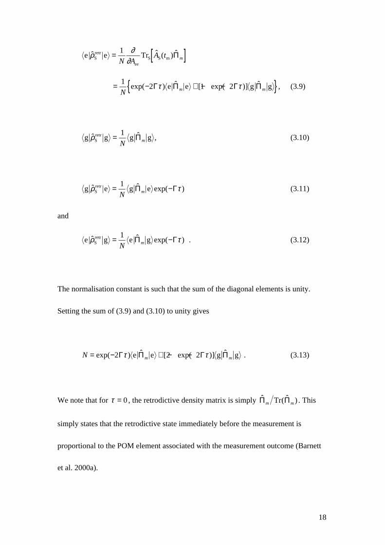
The normalisation constant is such that the sum of the diagonal elements is unity.

Setting the sum of (3.9) and (3.10) to unity gives

N m m= − + − −exp( ) ˆ [ exp( )] ˆ2 2 2Γ Π Γ Πτ τe e g g . (3.13)

We note that for τ = 0, the retrodictive density matrix is simply ˆ ( ˆ )Π Πm mTr . This

simply states that the retrodictive state immediately before the measurement is

proportional to the POM element associated with the measurement outcome (Barnett

et al. 2000a).

19

As an illustration, we use this retrodictive density matrix to calculate the

probability Pprep e g( | ) that the excited state was prepared by an unbiased apparatus

which is capable of preparing the atom in the excited or ground states, if the atom is

detected to be in its ground state. Projecting the retrodictive density matrix onto the

preparation POM element e e gives for this probability the expression (3.9) with

Πm = g g . This gives the result (3.5) obtained previously by direct calculation.

The retrodictive density matrix gives us more than just the ground and excited

state probabilities. As an example, suppose that our measurement of the atom gave a

result corresponding to the superposition state θ θ θ= +( )cos( ) sin( )2 2g e .

Furthermore, let us suppose that we know that the atom was prepared in one of the

non-orthogonal states e and + = +( )e g 2 and that the prior probabilities for

these two states are p and 1− p respectively. How does our measurement result

change these probabilities? To answer this question we first calculate the retrodictive

density matrix associated with our measurement result for which the POM element is

ˆ cos( ) sin( ) cos( ) sin( )Πm = = +( ) +( )θ θ θ θ θ θ2 2 2 2g e g e . (3.14)

A little algebra then shows the retrodictive density matrix elements to be

20

e eSretrˆ

cos exp

cos expρ

θ τ

θ τ=

+ − −( )[ ] + − −( )[ ]

12

1 1 2 2

1 1 2

Γ

Γ, (3.15)

g gSretrˆ

cos

cos expρ

θ

θ τ=

+( )+ − −( )[ ]

12

1

1 1 2Γ (3.16)

and

g e e gSretr

Sretrˆ

sin exp

cos expˆρ

θ τ

θ τρ=

−( )+ − −( )[ ] =

12

1 1 2

Γ

Γ. (3.17)

The two possible preparation events are associated with the operators

Λe e e= p (3.18)

and

ˆ ( ) ( )Λ+ = − + + = − +( ) +( )112

1p p e g e g . (3.19)

The probabilities that the atom was prepared in the state e or + given that it was

subsequently observed to be in the state θ are

Pprep S Sretr

e

S Sretr

e

eTr

Tr( | )

ˆ ˆ

ˆ ˆ ˆθ

ρ

ρ=

[ ]+( )[ ]+

Λ

Λ Λ

=+ − −( )[ ]

+ − −( )[ ] + − −( ) − −( )p

p p

1 1 2 2

1 1 2 1 2

cos exp

cos exp ( )sin exp cos exp

θ τθ τ θ τ θ τ

ΓΓ Γ Γ

(3.20)

21

and

Pprep S Sretr

S Sretr

e

Tr

Tr( | )

ˆ ˆ

ˆ ˆ ˆ+ =

[ ]+( )[ ]

+

+

θρ

ρ

Λ

Λ Λ

=− + − −( )[ ] + −( )

+ − −( )[ ] + − −( ) − −( )( ) cos exp sin exp

cos exp ( )sin exp cos exp

1 1 1 2 2

1 1 2 1 2

p

p p

θ τ θ τθ τ θ τ θ τ

Γ ΓΓ Γ Γ

. (3.21)

For τ = 0 , these probabilities are

Pp

p pprep e( | )

( cos )( cos ) ( )( sin )

θ θθ θ

= −− + − +

11 1 1

, (3.22)

Pp

p pprep( | )

( )( sin )( cos ) ( )( sin )

+ = − +− + − +

θ θθ θ

1 11 1 1

. (3.23)

These values agree with those obtained using Bayes’ theorem directly (Barnett et al

2000a),

PP

P

p

p pprep e

e, e

e( | )

( )( ) ( )

θ θθ

θθ θ

= =+ − +

2

2 21

(3.24)

PP

P

p

p pprep

e( | )

( , )( )

( )

( )+ = + =

− ++ − +

θ θθ

θθ θ

1

1

2

2 2 . (3.25)

22

For τ → ∞ , the probabilities reduce to P pprep e( | )θ = and P pprep( | )+ = −θ 1 , that is,

the prior probabilities. This tells us that, after a long time, the measurement gives us

no additional information about the initially prepared state.

3.2. Incoherently excited atom

We now consider the case of our two-level atom coupled to a thermal field of mean

occupation number n . This modifies the master equation governing the evolution of

the density matrix (Barnett and Radmore 1997) and in place of (3.8) we obtain

ˆ ( )A tS m =

e e ee ggAn

nn

n

nA

n

nn

2 12 2 1

12 1 2 1

1 2 2 1+

+ − +( ) ++

++

− − +( )[ ]

exp ( ) exp ( )Γ Γτ τ

+ ++

++

− +( )

+ ++

− − +( )[ ]

g g gg eeAn

n

n

nn A

n

nn

12 1 2 1

2 2 11

2 11 2 2 1exp ( ) exp ( )Γ Γτ τ

+ − +( ) + − +( )e g g eeg geA n A nexp ( ) exp ( )2 2 1 2 2 1Γ Γτ τ . (3.26)

The retrodictive density matrix elements can again be found by differentiation using

(2.8). This procedure gives

23

e eSretrρ = 1

2 11

2 12 2 1

N

n

n

n

nnme eˆ exp ( )Π Γ

++ +

+− +( )

τ

+ ++

− − +( )[ ]g gˆ exp ( )Π Γm

n

nn

12 1

1 2 2 1τ , (3.27)

g g g gSretrˆ ˆ exp ( )ρ τ= +

++

+− +( )

1 12 1 2 1

2 2 1N

n

n

n

nnmΠ Γ

++

− − +( )[ ]e eˆ exp ( )Π Γm

n

nn

2 11 2 2 1τ , (3.28)

g e g eSretrˆ ˆ exp ( )ρ τ= − +( )1

2 1N

nmΠ Γ (3.29)

and

e g e gSretrˆ ˆ exp ( )ρ τ= − +( )1

2 1N

nmΠ Γ . (3.30)

The normalisation constant is

Nn

n nnm=

++

+− +( )

e eˆ exp ( )Π Γ22 1

12 1

2 2 1τ

+ ++

−+

− +( )

g gn

n nnm

ˆ exp ( )Π Γ2 22 1

12 1

2 2 1τ . (3.31)

For τ → ∞ , it is clear that the retrodictive density operator tends to one half of the

identity operator, corresponding to no information about the initially prepared state.

This happens for all measured states because the thermal radiation can cause

24

absorption so that it is possible to prepare the atom in its ground state and to find it

later in its excited state. Figure 1 shows the predictive and retrodictive diagonal

density matrix elements for an atom respectively prepared or measured to be in its

excited state. The predictive density matrix elements rapidly decay to their steady

state form for which the ratio of the excited and ground state probabilities is

n n( )1+ . The retrodictive diagonal density matrix elements tend to the value 1/2 for

long time intervals τ .

3.3. Coherently driven atom

In our final example the atom is resonantly driven by an intense laser field. It is well

known that such a system exhibits Rabi oscillations at a frequency

Ω Γ= −( / ) /V 2 2 1 24 where V is proportional to the laser field strength and Γ is the

atomic spontaneous decay rate. The (interaction picture) Hamiltonian describing the

coupling between the atom and the laser field is

ˆ ˆ ˆ ,HV= +( )+ −2

σ σ (3.32)

where σ + = e g and σ − = g e . The reduced, predictive density operator for the

atom satisfies the master equation

25

∂∂

ρ σ σ ρ σ ρ σ σ σ ρ ρ σ σt

iVˆ ˆ ˆ , ˆ ˆ ˆ ˆ ˆ ˆ ˆ ˆ ˆ ˆ

Spred

Spred

Spred

Spred

Spred= − +( )

+ − −[ ]+ − − + + − + −22Γ . (3.33)

The solution for the predictive reduced density operator at the measurement time may

be written in the form

ˆ ( ) ˆ ( ) ˆ ( ) ˆ ( ) ˆρ τ σ τ σ τ σSpred

mt u v w= + + +[ ]12

1 1 2 3 , (3.34)

where 1= +e e g g is the unit operator on the space of the atom. The Pauli

operators σ1 = +e g g e, ˆ ( )σ 2 = −i g e e g and σ 3 = −e e g g represent

respectively the real and imaginary parts of the dipole moment and the atomic

inversion. The functions u v( ), ( )τ τ and w( )τ are the expectation values of ˆ , ˆσ σ1 2 and

σ 3 respectively at time τ after preparation and have the values (Barnett and Radmore

1997)

u u( ) ( )exp( )τ τ= −0 Γ (3.35)

vV

V V v V( ) exp( / )[( ) ( ) ]cos( )(τ τ τ=+

+ − + −12

2 3 2 2 0 22 22 2

ΓΓ Γ Γ Γ Ω

+ Ω Γ Γ Γ Ω− − + + − +1 2 2 23 2 0 0 2[ ( )( ( ) ( ) / )]sin )V V Vw v τ (3.36)

wV

V w( ) exp( / )[ ( ) ( )]cos(τ τ τ=+

− + − + +12

2 3 2 2 2 02 22 2 2 2

ΓΓ Γ Γ Γ Ω

26

+ − + + + −−Ω Γ Γ Γ Γ Ω1 2 2 2 22 2 2 0 0 2[ ( / ) ( )( ( ) ( ) / )]sin )V V Vv w τ . (3.37)

The excited and ground state matrix elements can be found from the master equation

solution (3.34) using

e eSpred

p eeˆ ( ) [ ( )]/ρ t A w= = +1 0 2 (3.38)

g gSpred

p ggˆ ( ) [ ( )]/ρ t A w= = −1 0 2 (3.39)

e gSpred

p egˆ ( ) [ ( ) ( )]/ρ t A u iv= = −0 0 2 (3.40)

g eSpred

p geˆ ( ) [ ( ) ( )]/ρ t A u iv= = +0 0 2. (3.41)

These can be substituted into (3.34)-(3.37) which allows us to calculate the

retrodictive density matrix elements according to (2.8). The calculations are

somewhat lengthy to reproduce in detail, so we shall concentrate on the results for a

few specific measurement POM elements.

27

We first study the case where the atom is detected to be in its excited state, so

the measurement POM element is Πm = e e. The retrodictive matrix elements are

then

e eSretr

ee

ˆ ( )( )

exp / [( )cosρ ∂∂

τ τ= +

=+

+ −( ) +12

11

2 23 2 42 2

2 2 2

N

w t

A N VV V

ΓΓ Γ Ω

− +ΓΩ

Γ Ω2

5 42 2( )sin ]V τ , (3.42)

g gSretrˆ

( )exp( / ) cos( ) sin( )ρ τ τ τ=

+− − +

V

N V

2

2 22 21 3 2

32Γ

Γ Ω ΓΩ

Ω , (3.43)

e g g eSretr

Sretrˆ ˆ exp( / )sin( )ρ ρ τ τ= − = − −iV

N23 2

ΩΓ Ω , (3.44)

where the normalisation constant is 112

+ +

∂ τ∂

∂ τ∂

w

A

w

A

( ) ( )

ee gg

. The evolution of the

predictive and retrodictive matrix elements for this system is shown in figure 2. In the

retrodictive case the diagonal matrix elements show Rabi oscillations which decay to

the “no information” level of 1/2. The off-diagonal elements decay to zero as

expected. This corresponds to a loss of coherence information about the system a

long time in the past. Similar behaviour is found for Πm = g g .

Suppose instead that the atom is measured in the superposition 12

e g+( )i ,

which gives ˆ ˆΠm = +( )12

1 2σ . The retrodictive matrix elements are

e eSretrρ = +

+

12

112

22 2N VV

ΓΓ

28

− − + +

exp( / ) cos( ) ( )sin( )3 2 2 52 2Γ Γ ΩΩ

Γ Ωτ τ τVV

V , (3.45)

g gSretrρ = +

+

12

112

22 2N VV

ΓΓ

− − + −

exp( / ) cos( ) ( )sin( )3 2 2 2 2Γ Γ ΩΩ

Γ Ωτ τ τVV

V , (3.46)

e g g eSretr

Sretrˆ ˆ exp( / )

cos( ) sin( )ρ ρ τ τ τ= − = − − +

i

N

3 22 2

Γ Ω ΓΩ

Ω ,

(3.47)

with Nv

A

v

A= + +

1

12

∂ τ∂

∂ τ∂

( ) ( )

ee gg

. These are shown in figure 3, along with the

corresponding predictive evolution. At the measurement time the retrodictive diagonal

matrix elements take their long-time values of 1/2. The off-diagonal matrix elements

are pure imaginary, and so they undergo Rabi oscillations. These elements couple to

the diagonal matrix elements so that we also see oscillations in the diagonal density

matrix elements.

Suppose now that the atom is measured to be in the superposition

12

e g+( ), so that the measurement POM element, ˆ ˆΠm = +( )12

1 1σ , contains only

the real part of the dipole matrix element. In this case the retrodictive matrix elements

are much simpler,

e e g gSretr

Sretrˆ ˆρ ρ= = 1

2, (3.48)

e g g eSretr

Sretrˆ ˆ exp( )ρ ρ τ= = −1

2Γ . (3.49)

29

Here the diagonal matrix elements are time-independent. The reason is that the off-

diagonal matrix elements are purely real and so do not lead to Rabi oscillations, that is

u( )τ simply decays.

The predictive state of a driven two-level atom evolves forward in time

towards a steady state with an unchanging population inversion and imaginary dipole

matrix element. The expectation values of the Pauli operators ˆ , ˆσ σ1 2 and σ 3 for this

state are

u( )τ = 0, (3.50)

vV

V( )τ =

+2

22 2

ΓΓ

, (3.51)

wV

( )τ = −+2

2

2

2 2

ΓΓ

. (3.52)

If we were to perform a measurement showing the atom to be in this state then we

could calculate a corresponding retrodictive density operator. The diagonal and off-

diagonal matrix elements of this density operator are shown in figures 4a and 4b

respectively. The off-diagonal matrix elements have a non-zero imaginary part so the

retrodictive density matrix exhibits damped Rabi oscillations. The long time interval

limit of the retrodictive density operator is, once again, one half of the identity

operator, corresponding to providing no information about the initially prepared state.

30

4. Conclusions

The retrodictive formalism provides the means to evaluate preparation

probabilities given the results of some later measurement event. Our approach relies

on the introduction of a retrodictive state. This is a state assigned to the system prior

to the measurement, based on the measurement result. Immediately before the

measurement, this retrodictive state is simply the normalised POM element

corresponding to the measurement result (Barnett et al 2000a). Put more simply, the

retrodictive density operator is the state corresponding to the measurement result. If

the system is closed, that is isolated from its environment, then the change in time of

the retrodictive density operator is unitary. If, however, the system is coupled to an

unmonitored environment then we will lose information about the system through

coupling to the environment. This will mean in most cases that the retrodictive density

operator for long times prior to the measurement will tend to become proportional to

the identity operator. This is the zero information state and reflects the fact that our

measurement tells us nothing about the way the system was prepared long before the

measurement.

We have applied the formalism to retrodict from measured states of a two-

level atom interacting with the electromagnetic field. For an undriven atom, which

can only undergo spontaneous emission, we find that the diagonal elements tend to

the value 1/2 and the off-diagonal ones to zero. This reflects the fact that we can

31

obtain from the measurement no information about the system a long time before the

measurement. The only exception is if the atom is measured in its excited state. In this

case, the retrodictive density operator must be the excited state projector e e for all

times prior to the measurement. This is because there is no light to absorb and so the

atom could not have made a transition to the excited state from the ground state. With

this exception, the decay to “no information” is a general feature of retrodiction for

damped two-level atoms, both driven and undriven.

We have also performed retrodictive calculations for the incoherently and

coherently driven atom. The evolution of the retrodictive density matrices of both

systems is different in character from that of their predictive counterparts. In the

forward time direction an atom driven by an incoherent field relaxes to a steady state

predictive density operator with the ratio of the excited and ground state probabilities

of n n/( )+1 . The corresponding ratio for retrodictive evolution is unity. For the

coherently driven atom we find retrodictive Rabi oscillations which decay. Again the

predictive and retrodictive evolutions decay to different forms for long time intervals,

with the retrodictive state tending to the zero-information state with density operator

1 2.

32

Acknowledgements

We thank Prof. R. Loudon for helpful comments and for a careful reading of our

manuscript. This work was supported by the United Kingdom Engineering and

Physical Sciences Research Council and by the Australian Research Council.

33

Appendix A. Probability operator measures

A comprehensive discussion of a probability operator measure (POM) is given by

Helstrom (1976). Here we outline only the essential features.

In the predictive formalism we can use a POM as a mathematical

representation of a measuring device. The POM is a set of elements Πm , each of

which is a positive semi-definite operator associated with a different possible outcome

of a measurement. Πm is defined such that the probability of the outcome m from a

measurement of a system with a predictive density matrix ρpred at the time of

measurement is given by Tr pred[ ˆ ˆ ]ρ Πm . The total probability for all possible outcomes

must be unity. Thus

Tr Trpred pred[ ˆ ˆ ] [ ˆ ˆ ]ρ ρΠ Πmm m

m=∑ ∑

= 1. (A.1)

For this to be true for all ρpred, normalisation of the trace of ρpred to unity requires

mm∑ Π to equal the unit operator.

A measurement that yields no information may be considered as a

measurement with only one possible outcome, for example a zero meter reading, for

34

all ρpred. Normalisation of the POM as above requires the corresponding single

element to be the unit operator.

We can also use a POM with elements Ξp as a mathematical description of an

unbiased preparation device. In this case Tr[ ˆ ˆ ]ρ retrΞp is the a posteriori probability of

a preparation outcome p based on knowledge of the measurement outcome. This

probability is equal to that obtainable from the predictive formalism combined with

Bayes’ theorem (Barnett et al 2000a). If the preparation device is biased we work

instead with components Λ p of the a priori density matrix.

35

Appendix B. Alternative derivation of retrodictive density matrix

Here we outline an alternative method for finding the retrodictive density matrix for a

two-level atom coupled to the environment. We first expand the retrodictive density

operator for the atom in terms Pauli operators σ j with j = 1 2 3, , (Barnett and

Radmore 1997). The general form of this expansion is

ˆ ˆ ˆρ σSretr = +

∑1

21 u j j

j

(B.1)

where 1 is the unit operator on the space of the atom. Multiplying by (ˆ ˆ )1+ σ k and

tracing over the atom states we obtain

TrS Sretr[(ˆ ˆ ) ˆ ]1 1+ = +σ ρk ku . (B.2)

Thus from (2.5) we have

uN

t U Uk k m= + −11 1TrES E

predp[(ˆ ˆ ) ˆ ( ) ˆ ˆ ˆ ]†σ ρ Π

= + −11 1

NU t Uk mTrES E

predp[ ˆ (ˆ ˆ ) ˆ ( ) ˆ ˆ ]†σ ρ Π

= + −11 1

Ntk mTrS m[(ˆ ˆ )( ) ˆ ]σ Π (B.3)

where, because (ˆ ˆ ) /1 2+ σ k has the form of a density matrix, we can find

36

(ˆ ˆ )( )1+ σ k tm = +TrE Epred

p[ ˆ (ˆ ˆ ) ˆ ( ) ˆ ]†U t Uk1 σ ρ (B.4)

from the appropriate master equation. Indeed the values of (ˆ ˆ )( )1+ σ k tm can be

obtained immediately from the general expressions given by Barnett and Radmore

(1997), that is, equations (3.35)-(3.37) with values of u v( ), ( )0 0 and w( )0 chosen as

0 or 1 as appropriate. Inserting these into (B.1) gives the retrodictive density matrix

in the form

ˆ ˆ [(ˆ ˆ )( ) ˆ ] ˆρ σ σSretr

S mTr= + + −

∑1

21

11 1

Ntj m j

j

Π . (B.5)

Finally we note that the expression for N, which is given by the denominator of (2.5)

can be written as

N U t U m= ⊗TrES Epred

p[ ˆ ˆ ( ) ˆ ˆ ˆ ]†ρ 1 Π

= TrS m[ˆ( ) ˆ ]1 t mΠ (B.6)

where, because ˆ /1 2 has the form of a density operator, we can find ˆ( )1 tm =

TrE Epred

pˆ ˆ ( ) ˆ ˆ †U t Uρ ⊗[ ]1 from the same master equation as used above.

37

References

Aharonov Y, Bergman P G and Lebowitz J L 1964 Phys. Rev. 134 B1410

Barnett S M and Radmore P M 1997 Methods in Theoretical Quantum Optics

(Oxford: Oxford University Press)

Barnett S M and Pegg D T 1999 Phys. Rev. A 60 4965

Barnett S M, Pegg D T and Jeffers J 2000a J. Mod. Opt. (in press)

Barnett S M, Pegg D T, Jeffers J, Jedrkiewicz O and Loudon R 2000b Phys. Rev. A

(in press)

Belinfante F J 1975 Measurements and Time Reversal in Objective Quantum Theory

(Oxford: Pergamon Press)

Box G E P and Tiao G C 1973 Bayesian inference in statistical analysis (Sydney:

Addison-Wesley), p. 10

Helstrom, C W 1976 Quantum Detection and Estimation Theory (New York:

Academic Press)

Pegg D T and Barnett S M 1999 J. Opt. B: Quantum Semiclass. Opt. 1 442

Penfield R H 1966 Am. J. Phys. 34, 422

38

Figure Captions

Fig. 1. Incoherently excited atom with a mean thermal occupation number of n = 1.

(a) Predictive diagonal density matrix elements plotted against time for an atom

initially prepared in the excited state. (b) Retrodictive diagonal density matrix

elements for an atom measured to be in the excited state. The solid and dashed curves

are the excited and ground state matrix elements respectively. The time τ, measured in

units of the atomic state lifetime, is the interval between preparation and

measurement. Note that in all figures, the preparation time is to the left of the

measurement time. This means that retrodictive density matrix elements are plotted

with τ increasing to the left.

Fig. 2. Coherently driven atom with V = 4Γ . (a) Predictive diagonal density matrix

elements for an initially excited atom, and (b) retrodictive diagonal density matrix

elements for an atom measured to be in the excited state. The solid and dashed curves

are the excited and ground state matrix elements respectively. (c) Imaginary part of

the predictive and (d) retrodictive off-diagonal matrix elements for the same systems

as (a) and (b). The solid and dashed curves are the imaginary parts of e gSretrρ and

g eSretrρ respectively. The real parts are zero.

39

Fig. 3. Coherently driven atom with V = 4Γ . (a) Predictive diagonal density matrix

elements for an atom initially in the superposition e g+( )i 2 , and (b) retrodictive

diagonal density matrix elements for an atom measured to be in the same

superposition. (c) Imaginary part of the predictive and (d) retrodictive off-diagonal

matrix elements for the same systems as (a) and (b). The solid and dashed curves

represent the same quantities as in figure 2.

Fig. 4. Coherently driven atom with V = 4Γ . (a) Retrodictive diagonal density matrix

elements for an atom measured to be in the predictive steady state. (b) Retrodictive

off-diagonal matrix elements for the same system. The solid and dashed curves

represent the same quantities as in figures 2b and 2d.

0

0.2

0.4

0.6

0.8

1

0.2 0.4 0.6 0.8 1τ/Γ

Diagonal Elements

0.2

0.4

0.6

0.8

1

1 0.8 0.6 0.4 0.2 0τ/Γ

Diagonal Elements

0

0.2

0.4

0.6

0.8

1

0 1 2 3 4 5τ/Γ

Diagonal Elements

0.2

0.4

0.6

0.8

1

5 4 3 2 1 0τ/Γ

Diagonal Elements

-0.4

-0.2

0

0.2

0.4

1 2 3 4 5τ/Γ

Off-diagonal Elements

-0.4

-0.2

0

0.2

0.4

5 4 3 2 1τ/Γ

Off-diagonal Elements

0.2

0.3

0.4

0.5

0.6

0.7

0.8

1 2 3 4 5τ/Γ

Diagonal Elements

0.2

0.3

0.4

0.5

0.6

0.7

0.8

5 4 3 2 1τ/Γ

Diagonal Elements

-0.4

-0.2

0

0.2

0.4

1 2 3 4 5τ/Γ

Off-diagonal Elements

-0.4

-0.2

0

0.2

0.4

5 4 3 2 1τ/Γ

Off-diagonal Elements

0.4

0.5

0.6

5 4 3 2 1 0τ/Γ

Diagonal Elements

-0.2

-0.1

0

0.1

0.2

5 4 3 2 1τ/Γ

Off-diagonal Elements