
Entanglement distribution over 150 km in wavelength division ...
Upload
khangminh22Category
view
4download
0
Efficient Tomography and EntanglementDetection of Multiphoton States
Christian Schwemmer
Munchen, August 2015


Efficient Tomography and EntanglementDetection of Multiphoton States
Christian Schwemmer
Munchen, August 2015


Efficient Tomography and EntanglementDetection of Multiphoton States
Christian Schwemmer
Dissertationan der Fakultat fur Physik
der Ludwig-Maximilians-UniversitatMunchen
vorgelegt vonChristian Michael Schwemmer
aus Forrenbach
Munchen, August 2015

Erstgutachter: Prof. Dr. WeinfurterZweitgutachter: Prof. Dr. Belen ParedesTag der mundlichen Prufung: 30.9.2015

Fur meine Mutter.


Landscape with Blind Orion Searching for the Sun, Nicolas Poussin, 1658.


Ist der Zwerg auf den Schultern des Riesen nichtimmer großer, als der Riese selbst?
Johann Gottfried von Herder,Abhandlung uber den Ursprung der Sprache


Contents
Abstract xvii
Zusammenfassung xix
1. Introduction 1
2. Fundamentals of quantum information theory 52.1. Single qubits . . . . . . . . . . . . . . . . . . . . . . . . . . . . . . 6
2.1.1. From classical bits to quantum bits . . . . . . . . . . . . . 62.1.2. Single-qubit manipulation and discrimination . . . . . . . 9
2.2. Multiqubit states and entanglement . . . . . . . . . . . . . . . . . 102.2.1. Multiple qubits . . . . . . . . . . . . . . . . . . . . . . . . 102.2.2. Classification of multiqubit states . . . . . . . . . . . . . . 122.2.3. Entanglement detection . . . . . . . . . . . . . . . . . . . 172.2.4. Entanglement measures . . . . . . . . . . . . . . . . . . . 21
2.3. Experimental realization of photonic multiqubit states . . . . . . 252.3.1. Spontaneous parametric down conversion . . . . . . . . . . 252.3.2. Linear optical setups . . . . . . . . . . . . . . . . . . . . . 29
3. Entanglement detection by correlation measurements 353.1. Optimized state-independent entanglement detection . . . . . . . 36
3.1.1. Experimentally friendly entanglement criterion . . . . . . . 363.1.2. Experimental Schmidt decomposition . . . . . . . . . . . . 383.1.3. Decision tree . . . . . . . . . . . . . . . . . . . . . . . . . 40
3.2. No correlation states . . . . . . . . . . . . . . . . . . . . . . . . . 423.2.1. States and antistates . . . . . . . . . . . . . . . . . . . . . 433.2.2. Family of genuine entangled no correlation states . . . . . 44
3.3. Publications . . . . . . . . . . . . . . . . . . . . . . . . . . . . . . 48P3.1. Experimental Schmidt Decomposition and State Indepen-
dent Entanglement Detection . . . . . . . . . . . . . . . . 50P3.2. Optimized state-independent entanglement detection based
on a geometrical threshold criterion . . . . . . . . . . . . . 57P3.3. Genuine Multipartite Entanglement without Multipartite
Correlations . . . . . . . . . . . . . . . . . . . . . . . . . . 68
ix

Contents
4. Quantum state tomography 854.1. Standard tomography . . . . . . . . . . . . . . . . . . . . . . . . . 86
4.1.1. Projector-based complete tomography . . . . . . . . . . . 874.1.2. Pauli tomography scheme . . . . . . . . . . . . . . . . . . 894.1.3. Physicality constraint . . . . . . . . . . . . . . . . . . . . . 904.1.4. Comparison of algorithms . . . . . . . . . . . . . . . . . . 93
4.2. Partial tomography schemes . . . . . . . . . . . . . . . . . . . . . 954.2.1. Compressed sensing . . . . . . . . . . . . . . . . . . . . . . 954.2.2. Permutationally invariant tomography . . . . . . . . . . . 964.2.3. Compressed sensing in the permutationally invariant subspace102
4.3. Publications . . . . . . . . . . . . . . . . . . . . . . . . . . . . . . 102P4.1. Permutationally Invariant Quantum Tomography . . . . . 104P4.2. Experimental Comparison of Efficient Tomography Schemes
for a Six-Qubit State . . . . . . . . . . . . . . . . . . . . . 112P4.3. Permutationally invariant state reconstruction . . . . . . . 120
5. Systematic errors of standard quantum state estimation 1455.1. Origin of unphysical density matrices . . . . . . . . . . . . . . . . 1465.2. Constrained state estimation . . . . . . . . . . . . . . . . . . . . . 149
5.2.1. Flaws of constrained state estimation . . . . . . . . . . . . 1495.2.2. Biasedness and physicality . . . . . . . . . . . . . . . . . . 152
5.3. Publications . . . . . . . . . . . . . . . . . . . . . . . . . . . . . . 153P5.1. Systematic Errors in Current Quantum State Tomography
Tools . . . . . . . . . . . . . . . . . . . . . . . . . . . . . . 155
6. Conclusions 163
A. Appendix 167A.1. Additional remarks on convex optimization . . . . . . . . . . . . . 167
A.1.1. Maximum likelihood . . . . . . . . . . . . . . . . . . . . . 167A.1.2. Least squares . . . . . . . . . . . . . . . . . . . . . . . . . 168A.1.3. Barrier term . . . . . . . . . . . . . . . . . . . . . . . . . . 169A.1.4. Implementation . . . . . . . . . . . . . . . . . . . . . . . . 169
A.2. Measurement settings for PI tomography . . . . . . . . . . . . . . 169
Publication list 173
Bibliography 177
Acknowledgments 201
Curriculum vitae 203
x

List of Figures
2.1. Bloch sphere . . . . . . . . . . . . . . . . . . . . . . . . . . . . . . 72.2. SLOCC classes for three qubits . . . . . . . . . . . . . . . . . . . 142.3. Graph states . . . . . . . . . . . . . . . . . . . . . . . . . . . . . . 162.4. Four-qubit symmetric Dicke states . . . . . . . . . . . . . . . . . . 172.5. Entanglement witnesses . . . . . . . . . . . . . . . . . . . . . . . 202.6. Geometric measure of entanglement . . . . . . . . . . . . . . . . . 242.7. Spontaneous parametric down conversion . . . . . . . . . . . . . . 272.8. Photon source based on a UV enhancement cavity . . . . . . . . . 292.9. Building blocks of linear setups . . . . . . . . . . . . . . . . . . . 32
3.1. Schmidt decomposition . . . . . . . . . . . . . . . . . . . . . . . . 393.2. Schmidt decomposition in practice . . . . . . . . . . . . . . . . . . 403.3. Two-qubit decision tree . . . . . . . . . . . . . . . . . . . . . . . . 413.4. Efficiency of the two-qubit decision tree . . . . . . . . . . . . . . . 423.5. Entanglement of no-correlation states . . . . . . . . . . . . . . . . 453.6. Vanishing correlations and predictability . . . . . . . . . . . . . . 46
4.1. Convergence of fit algorithms . . . . . . . . . . . . . . . . . . . . 944.2. Convergence of compressed sensing . . . . . . . . . . . . . . . . . 964.3. Number of PI correlations . . . . . . . . . . . . . . . . . . . . . . 974.4. Measurement operators for PI tomography . . . . . . . . . . . . . 994.5. Block diagonal decomposition of PI operators . . . . . . . . . . . 101
5.1. Unphysical result due to an odd number of counts . . . . . . . . . 1465.2. Unphysicality and statistics . . . . . . . . . . . . . . . . . . . . . 1485.3. Biased fidelity estimation . . . . . . . . . . . . . . . . . . . . . . . 1505.4. Overestimation of negativity . . . . . . . . . . . . . . . . . . . . . 1515.5. Effect of fitting . . . . . . . . . . . . . . . . . . . . . . . . . . . . 1515.6. Biasedness of constrained state estimation . . . . . . . . . . . . . 152
xi

List of Figures
xii

List of Tables
2.1. Angle settings for Pauli measurements . . . . . . . . . . . . . . . 33
A.1. Optimized settings for four-qubit PI tomography . . . . . . . . . . 170A.2. Randomly chosen settings for four-qubit PI tomography . . . . . . 170A.3. Optimized settings for six-qubit PI tomography . . . . . . . . . . 171
xiii

List of Tables
xiv

Abbreviations
APD avalanche photo diode
BBO β-barium-borate
BS beam splitter
CS compressed sensing
FPGA field programmable gate array
FWHM full width at half maximum
GHZ Greenberger-Horne-Zeilinger
LBO lithium-triborate
LHV local hidden variable
LOCC local operations and classical communication
LU local unitary
HWP half-wave plate
PBS polarizing beam splitter
PI permutationally invariant
POVM positive operator valued measure
PPT positive partial transposition
PVM projector valued measure
QWP quater-wave plate
SHG second harmonic generation
SLOCC statistical local operations and classical communication
SPDC spontaneous parametric down-conversion
Ti:Sa titanium:sapphire
UV ultraviolet
YVO yttrium-vanadate
xv

Abbreviations
xvi

Abstract
Quantum mechanics is without doubt one of the most successful theories in thehistory of science. Yet, due to its counter intuitive predictions, it still challengesmany physicists. In this context, as a consequence of the principle of superposi-tion, especially the phenomenon of entanglement has to be named. Although en-tanglement lacks any classical interpretation, it is nonetheless at the heart of novelmethods for data processing like quantum communication or quantum computa-tion. In an interdisciplinary effort of mathematics, computer science and physics,researchers from the respective fields try to better understand and characterizemultipartite entanglement and to pave the way for its practical application.
In this work, the focus is on the development of appropriate tools to analyzeand characterize multipartite entangled states as well as their experimental imple-mentation by means of polarization encoded multiphoton states. More precisely,Bell states, and especially symmetric Dicke states with up to six photons are in-vestigated. In order to generate these states, photon sources based on the processof spontaneous parametric down-conversion are used.
In the first part of this work, two schemes that allow to detect entanglement oftwo- and multiqubit states with possibly few correlation measurements are pre-sented and experimentally implemented. In the first scheme, the state is trans-formed into the Schmidt basis such that entanglement can be verified with at mostthree correlation measurements. The second scheme makes use of the principle ofcorrelation complementarity in order to perform only those measurements whichare most advantageous for entanglement detection. The scheme can be representedin a compact form called decision tree which determines the next measurement tobe carried out depending on the result of the previous measurement. In anotherexperiment, it is investigated what kind of correlations are typical for genuineN -partite entanglement. Interestingly, it can be shown that N -partite entangle-ment does not necessitate the presence of correlations between all parties. This isdemonstrated on the example of photonic three- and five-qubit states.
In the second part of this work, permutationally invariant tomography is pre-sented which is a novel partial tomography scheme for the efficient analysis ofsymmetric multiqubit states. In the experimental implementation of this scheme,the emphasis was to increase the count rates thus far that full tomography ofsix-photon states became possible. In experiments with four- and six-photonsymmetric Dicke states, various tomography schemes, like full tomography andpermutationally invariant tomography, were compared against each other and it
xvii

Abstract
was shown that the results of the respective schemes are compatible. In this con-text, it is of utmost importance that not only the measurement scheme itself isscalable but also subsequent data analysis. This can be achieved by a speciallyadopted algorithm which, on the one hand, utilizes the symmetry of the stateto be analyzed, and, on the other hand, resorts to highly efficient methods fromconvex optimization. It was also observed that data analysis itself can cause sys-tematic errors of the final result. As it turned out, for the measurement statisticsthat are typical of today’s multiqubit experiments, the systematic errors are ofthe same magnitude as the statistical errors and can therefore not be ignored.
xviii

Zusammenfassung
Die Quantenmechanik zahlt zweifelsohne zu einer der erfolgreichsten wissenschaft-lichen Theorien, die aber aufgrund ihrer kontraintuitiven Vorhersagen viele Phy-siker nach wie vor herausfordert. In diesem Zusammenhang ist insbesondere dasaus dem Superpositionsprinzips folgende Phanomen der Verschrankung zu nen-nen. Auch wenn sich Verschrankung klassisch nicht verstehen lasst, so bildet siedoch das Herzstuck fur neuartige Methoden der Datenverarbeitung wie Quanten-kommunikation oder Quantenrechnen. In einer interdisziplinaren Anstrengung vonMathematik, Informatik und Physik versuchen Forscher Vielteilchenverschrank-ung besser zu verstehen und zu charakterisieren, sowie fur die praktische Anwen-dung nutzbar zu machen.
Die vorliegende Arbeit beschaftigt sich mit der Entwicklung von geeigneten Me-thoden zur Analyse und Charakterisierung von vielteilchenverschrankten Zustan-den sowie deren experimentellen Realisierung anhand von verschiedenen polari-sationskodierten Mehrphotonenzustanden. Hierbei werden, neben Bell-Zustanden,insbesondere symmetrische Dicke-Zustande mit bis zu sechs Photonen untersucht.Als Photonenquelle wird dabei der Prozess der spontanen parametrischen Fluo-reszenz in verschiedenen Varianten verwendet.
Im ersten Teil dieser Arbeit werden zwei Methoden vorgestellt und experimen-tell implementiert, die es erlauben die Verschrankung von Zwei- und Mehrqubit-Zustanden mit moglichst wenigen Korrelationsmessungen nachzuweisen. Hierbeiberuht die erste Methode auf einer Transformation des Zustandes in die Schmidt-basis, wodurch sich im Anschluss Verschrankung mit maximal drei Korrelations-messungen nachweisen lasst. Die zweite Methode verwendet das Prinzip der Kor-relationskomplementaritat, um nur die Messungen durchzufuhren, die am vor-teilhaftesten sind um Verschrankung moglichst schnell nachzuweisen. Das Sche-ma lasst sich kompakt in Form eines Entscheidungsbaumes ausdrucken, der dieals nachstes durchzufuhrende Messung in Abhangigkeit des vorherigen Messer-gebnisses festlegt. In einem weiteren Experiment wird untersucht, welche Artenvon Korrelationen fur genuine N -Teilchenverschrankung notwendig sind. Dabeikann gezeigt werden, dass fur N -Teilchenverschrankung interessanterweise keineN -Parteien-Korrelationen zwingend erforderlich sind. Dies wird exemplarisch furphotonische Zustande mit drei und funf Qubits demonstriert.
Im zweiten Teil dieser Arbeit wird mit permutationsivarianter Tomographie ei-ne neuartige partielle Tomographiemethode vorgestellt, die eine effiziente Unter-suchung von symmetrischen Multiqubitzustanden erlaubt. In der experimentellen
xix
Zusammenfassung
Umsetzung liegt der Schwerpunkt hierbei insbesondere darauf, durch viele Detail-verbesserungen die Zahlraten soweit zu erhohen, dass eine vollstandige Zustands-analyse auch fur sechs Photonen moglich ist. In Experimenten mit symmetrischenDicke-Zustanden mit vier und sechs Photonen werden verschiedene tomographi-schen Methoden, darunter vollstandige Tomographie und permutationsinvarianteTomographie, miteinander verglichen. Dabei konnte gezeigt werden, dass alle Me-thoden kompatible Resultate liefern. Hier ist es insbesondere wichtig, dass nichtnur das Messschema selbst skalierbar ist, sondern auch die anschließende Auswer-tung der Daten. Dies wird durch einen speziell angepassten Algorithmus erreicht,der einerseits die Symmetrie des zu analysierenden Zustandes ausnutzt und an-dererseits auf hocheffiziente Methoden der konvexen Optimierung zuruckgreift. Indiesem Zusammenhang wurde auch untersucht, in wieweit die Datenauswertungselbst zu systematischen Fehlern fuhren kann. Wie sich herausstellte, sind beifur Multiqubitexperimenten typischen Messstatistiken die systematischen Fehlervon der gleichen Großenordnung wie die statistischen und konnen folglich nichtvernachlassigt werden.
xx
1. Introduction
The nineteenth century witnessed an unprecedented deepening in the understand-ing of the laws of physics culminating in the theories of electrodynamics and ther-modynamics. Together with the theory of classical mechanics, these theories formthe core of what is today called classical physics. However, at the turn of thecentury, there were, due to refined experimental techniques, more and more newfindings that could not be understood within the framework of classical physics.Especially, black body radiation, the stability of atoms and the spectra of atomslacked a satisfactory explanation. In 1900, when Max Planck [1] derived the ra-diation law, the first of these puzzles could by resolved, thereby constituting thebirth of quantum mechanics. In the first decades of the twentieth century, quan-tum mechanics developed further and comprehensive explanations for all of theabove mentioned problems could be given. Despite its tremendous success, therewas no consensus about the correct interpretation of the new theory, as shown bythe historical debate between Nils Bohr and Albert Einstein [2, 3].
Especially, the probabilistic nature of quantum mechanics lead to a strong feel-ing of unease in Albert Einstein. In 1935, he made his concerns explicit by pub-lishing a seminal paper [4] together with Boris Podolski and Nathan Rosen. Inthis paper, the authors consider a state that was later called “entangled” by ErwinSchrodinger [5]. Entangled states allow for situations where, although the systemas a whole is perfectly known, the knowledge about its individual subsystems canbe minimal. In such cases, the system can only be treated as a whole, even if itssubsystems are arbitrarily far separated. This lead Einstein and his coworkers tothe conclusion that quantum mechanics must be incomplete and they postulatedthe existence of additional, so-called hidden variables. For almost three decades,entanglement was mainly considered as a strange peculiarity of the theory whichis, at best, of philosophical interest but has no practical relevance.
This situation changed completely, when John Bell reformulated the originalargument of Einstein, Podolski and Rosen in a way that allowed to deduce exper-imentally testable predictions which differ from those of quantum mechanics [6].Over the years, these tests, which are now known under the term “Bell tests”,were further refined, but already the first experimental tests made a clear state-ment in favor of quantum mechanics [7–9]. Nonetheless, hidden variable theoriescould not be completely eradicated since all Bell tests that were performed up tonow have some “loopholes” which allow, at least in principle, for a classical in-terpretation. While certain loopholes have been closed separately [10, 11], at the
1

1. Introduction
time of writing, an experiment where all the loopholes are closed simultaneouslyis still missing. However, it is more than likely that such an experiment will becarried out in the near future [12–14].
Additionally to the these fundamental aspects, it was realized that quantummechanics also allows for novel approaches with respect to information process-ing [15, 16]. Examples for potential new applications with entanglement as akey resource comprise, to name just few, dense coding [17], quantum cryptogra-phy [18], quantum enhanced metrology [19] or quantum teleportation [20]. Forsome computational tasks, like, searching in huge databases [21] or factoring largenumbers [22], it could be shown that they can, at least in principle, be performedexponentially faster than classically.
Central to quantum information is the quantum bit, or shortly qubit [23], whichis the quantum mechanical analog of the classical bit. The main difference betweenqubits and their classical counterparts is that they cannot only be in the groundor the excited state of a two-level system but in any superposition of the two.Experimentally, qubits can be implemented with various physical systems, like,e.g., trapped atoms [24, 25], trapped ions [26], superconducting qubits [27–29], NVcenters in diamond [30], and photons [31]. Each of the different approaches has itsadvantages but also its specific drawbacks. For quantum computational problems,localized, well controllable systems like atoms, ions or superconducting qubitsseem to be preferable, whereas for quantum communication tasks where qubitshave to be exchanged over large distances, photons are the system of choice. In thelast years, due to refined experimental techniques, the number of entangled qubitswas constantly increasing [32–35]. However, despite of this enormous progress, itremains an open question whether it will be possible to control hundreds of qubitsone day and to really harness the power that lies within quantum computation. Inthis context, it is still an open issue how large a quantum system can grow beforeinherent decoherence, even arbitrarily small, induces a transition from quantumto classical [36, 37].
In this thesis, the polarization degree of freedom of photons was used for theexperimental implementation of qubits and to investigate various quantum infor-mation tasks. Photons are an ideal test system for proof-of-principle realizationsof many quantum information protocols [31] as they experience almost no deco-herence. However, the major advantage of photons is at the same time their worstdrawback, namely, that they practically do not interact with each other. Con-sequently, two-qubit gates as they are required for quantum computation cannotbe realized in a simple manner. This restriction could be overcome in 2001, whenEmanuel Knill, Raymond Laflamme, and Gerard Milburn presented a scheme foroptical quantum computing that requires only single-photon sources, linear opticalcomponents and photon number resolving detectors [38]. The original scheme waslater on further refined and could be reduced to the deterministic preparation ofspecific multipartite entangled quantum states together with suitable single-qubit
2

operations [39–43]. At the time of writing, the main drawback of optical quantumcomputation is still the lack of practical single-photon sources but the technicaldevelopment proceeds fast [44–48]. Until such sources are available, one has toresort, as also in this work, to the process of spontaneous parametric down con-version [49, 50] together with linear optical networks in order to prepare photonicmultiqubit states.
Although the number of qubits is still moderate in today’s multiqubit exper-iments, up to six in this work, full quantum state tomography, i.e., a completecharacterization of the state, becomes already a great challenge. The limit wherefull tomography becomes infeasible due to experimental restrictions, like set-upstability, drifts, measurement time etc. will soon be reached. Thus, it is of ut-most importance to find simple and experimentally friendly tools where relevantquantities about a quantum state, like, e.g., its overlap with respect to a targetstate, can be inferred from partial information. The research focus of this workis twofold. On the one hand, it is on the development and application of toolsfor entanglement detection from possibly few correlation measurements [51–53](the corresponding publications are included in this work as P3.1 and P3.2). Inthis context, also the connection between genuine N -partite entanglement and theexistence of N -partite correlations is investigated [54] (see publication P3.3). Onthe other hand, the focus is on the increase of rates such that full tomography ofa six-qubit state becomes possible and can be compared against highly efficienttomography protocols which require only partial information [55–58] (see publica-tions P4.1, P4.2 and P4.3). There, it was also observed that the standard analysistools for tomography can lead to systematic errors [59] (see publication P5.1).
For many entanglement criteria, it is required that the state to be characterizedis properly aligned with respect to the local measurement bases [60, 61], whichdoes not pose a problem, when all observers share a common reference frame. If,however, a common reference frame cannot be guaranteed, a situation that maylikely occur in quantum information protocols where the observers are far sepa-rated from each other, entanglement might therefore not be detected, althoughit is present. In order to overcome this problem, two different schemes are dis-cussed (see P3.1 and P3.2). The first one, which is designed for pure two-qubitstates, effectively performs a Schmidt decomposition [62] of the state. Then, aftera redefinition of the local measurement bases, entanglement can easily be verifiedwith a simple criterion [51] which requires at maximum three correlation mea-surements. The second scheme is more general and is based on the principle ofcorrelation complementarity [63], where the results of the performed correlationmeasurements determine which is the next measurement to be carried out.
In order to detect entanglement between N parties, one normally resorts toentanglement criteria which depend on correlations between all parties [51, 60, 64–71]. In this context, correlations are defined by the standard correlation functionas used in classical statistics and signal analysis [72, 73]. However, as first shown
3
1. Introduction
by Kaszlikowski et al. in [74], quantum mechanics allows for states that aregenuinely N -partite entangled, but lack N -partite correlations. At no surprise,these findings triggered a vivid discussion about the distinction between classicaland quantum correlations [75, 76]. In this work, the result by Kaszlikowski et al.is generalized and a constructive scheme is presented which allows to generate aninfinite family of genuinely N -partite entangled states with vanishing N -partitecorrelations. In three- and five-qubit experiments, such peculiar quantum stateswere prepared for the first time [54] (see also P3.3).
As already mentioned above, full quantum state tomography is not feasible forlarger systems. However, many prominent and highly relevant quantum statesbelong to subclasses of states which can be represented by few parameters. Forsuch states, efficient tomography schemes exist, like, e.g., tomography of matrixproduct states [77], compressed sensing [55] or permutationally invariant tomog-raphy [56]. As these schemes are to be applied in situations where full tomographycannot be performed, it is absolutely necessary to test these schemes against fulltomography for systems where this is still possible. In this work, full tomographyof a symmetric six-photon Dicke state [78, 79] was performed and the result wascompared with the results from compressed sensing, permutationally invariant to-mography and a combination of the two [58] (see publications P4.1 and P4.2). Forscalable tomography schemes, it is also crucial to have highly efficient algorithmsfor data analysis at hand [57] (see P4.3).
In every experimental situation one has to perform a thorough and carefulanalysis of all the errors that might influence the final result. Here, one has todistinguish between unavoidable statistical errors [80] and systematic errors, like,e.g., drifts of the experimental apparatus [81]. Interestingly, also data analysisitself can lead to systematic errors if additional constraints, like the physicality ofan estimated quantum state, are applied. In this context, the standard proceduresto analyze tomography data were investigated. There, it was observed that, fortypical count statistics of today’s multiqubit experiments, the deviations can beconsiderable [59] (see publication P5.1).
The thesis is structured as follows: In chapter 2, a short review of the founda-tions of quantum information is given and the notations used throughout this workare introduced. More precisely, the theoretical concepts of two- and multiqubitentanglement are explained together with the most relevant tools to detect andquantify entanglement. Additionally, the basic building blocks of the experimentsthat were performed in the course of this work are discussed. Then, in chapter 3,both theoretical and experimental results how entanglement can be detected in anexperimentally efficient way are presented. In chapter 4, novel methods for effi-cient state tomography are presented and compared against the standard method.Finally, in chapter 5, the standard tools for data analysis are reviewed, especiallywith respect to their reliability. The respective chapters also contain the relevantresearch papers that were written in the course of this work.
4

2. Fundamentals of quantuminformation theory
In this chapter, the basic concepts and tools required to describe and analyze singleand multiqubit systems are introduced. Section 2.1 starts with a formal definitionof what a qubit is [23] and discusses both the similarities and differences betweena classical and a quantum bit. Then, in section 2.2, systems consisting of morethan a single qubit are considered. As a consequence of the superposition princi-ple, such systems can be in a state without classical analog, a so-called entangledstate. After a formal definition of entanglement [82], several possibilities how toclassify entangled states are presented. More precisely, entangled states with morethan two qubits feature a rich hierarchical structure, i.e., they can be entangledin more than just one way [83].
If entanglement is to be used as a resource for practical applications, it is vital todetect and quantify its amount in an experimentally prepared state. Therefore, insection 2.2.3, several tools that allow to detect entanglement [84, 85] of a state arediscussed and in section 2.2.4, some well-known entanglement measures [86, 87]are listed.
In section 2.3, the last part of this chapter, the focus lies on the practical real-ization of multiphoton entangled states. It begins with a review of photon sourcesbased on the process of spontaneous parametric down-conversion (SPDC) [49, 50]as such photon sources are still the workhorse of today’s multiphoton experi-ments. Then, the basic building blocks to further process the generated photonsand to prepare the desired state are discussed. In detail, these building blocks arebeam splitters (BS), both polarizing and non-polarizing, phase shifters such ashalf (HWP) and quarter wave plates (QWP) and combinations thereof, e.g. forpolarization analysis.
In summary, this introductory chapter can be considered as a short review ofthe most relevant concepts and tools required to carry out experiments with mul-tiphoton entangled states. The discussion goes largely along the same line asin [88] and the introductory chapters of [89–91]. The chapter lays the necessaryfoundations to understand the experiments described in chapters 3 to 5.
5
2. Fundamentals of quantum information theory
2.1. Single qubits
2.1.1. From classical bits to quantum bits
In the following, the basic notation and concepts necessary to describe single two-level quantum systems are introduced. Such systems, called quantum bit or, forshort, qubit [23], are the quantum mechanical analog of the classical bit. Contraryto a classical bit, which can either be in the ground state 0 or in the excited state 1,a quantum bit can be in any superposition of these two states. Formally, a puresingle-qubit state is given by [62, 92–95]
|ψ〉 =1√
|α|2 + |β|2(α|0〉+ β|1〉) (2.1)
where |0〉 and |1〉 designate two orthogonal basis states of the Hilbert spaceH = C⊗2 and with complex numbers α and β. Here, and later on in thisthesis, the Dirac notation |·〉 will be used to discriminate quantum states fromclassical states. Since the state |ψ〉 has to be normalized, i.e. |〈ψ | ψ 〉|2 = 1, itcan be rewritten, up to a negligible global phase, as
|ψ(θ, φ)〉 = cosθ
2|0〉+ eiφ sin
θ
2|1〉. (2.2)
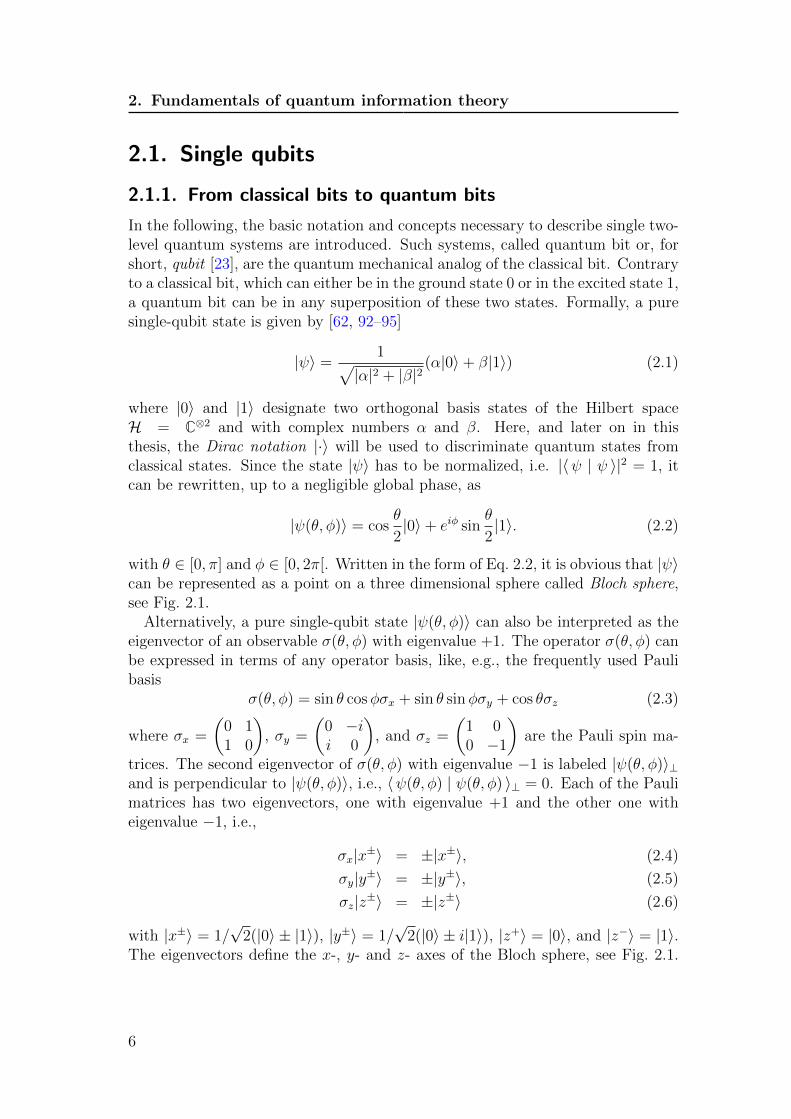
with θ ∈ [0, π] and φ ∈ [0, 2π[. Written in the form of Eq. 2.2, it is obvious that |ψ〉can be represented as a point on a three dimensional sphere called Bloch sphere,see Fig. 2.1.
Alternatively, a pure single-qubit state |ψ(θ, φ)〉 can also be interpreted as theeigenvector of an observable σ(θ, φ) with eigenvalue +1. The operator σ(θ, φ) canbe expressed in terms of any operator basis, like, e.g., the frequently used Paulibasis
σ(θ, φ) = sin θ cosφσx + sin θ sinφσy + cos θσz (2.3)
where σx =
(0 11 0
), σy =
(0 −ii 0
), and σz =
(1 00 −1
)are the Pauli spin ma-
trices. The second eigenvector of σ(θ, φ) with eigenvalue −1 is labeled |ψ(θ, φ)〉⊥and is perpendicular to |ψ(θ, φ)〉, i.e., 〈ψ(θ, φ) | ψ(θ, φ) 〉⊥ = 0. Each of the Paulimatrices has two eigenvectors, one with eigenvalue +1 and the other one witheigenvalue −1, i.e.,
σx|x±〉 = ±|x±〉, (2.4)
σy|y±〉 = ±|y±〉, (2.5)
σz|z±〉 = ±|z±〉 (2.6)
with |x±〉 = 1/√
2(|0〉 ± |1〉), |y±〉 = 1/√
2(|0〉 ± i|1〉), |z+〉 = |0〉, and |z−〉 = |1〉.The eigenvectors define the x-, y- and z- axes of the Bloch sphere, see Fig. 2.1.
6

2.1. Single qubits
Figure 2.1.: A pure quantum state |ψ(θ, φ)〉 can be represented as a point onthe surface of the Bloch sphere. The mixed states lie inside the sphere with thetotally mixed state 1/2 at the origin of the sphere. The x-, y- and z-axes of thecoordinate system are defined by the eigenvectors of the Pauli matrices σx, σyand σz.
Therefore, from now on, “measuring in the σx basis” will be used as a synonym forperforming projection measurements on the pair of orthogonal vectors |x+〉 and|x−〉. Correspondingly, the expressions “measuring in the σy basis” and “measur-ing in the σz basis” will be used.
As already mentioned, the points on the surface of the Bloch sphere can beinterpreted as pure quantum states. In addition, also the points lying inside thesphere can be associated with quantum states, the so-called mixed states, whichare states with a classical statistical distribution over pure states. A mixed statecannot be described by a state vector |ψ〉 anymore but, instead, by a densitymatrix
% =1∑i=0
pi |ψ(θi, φi) 〉〈ψ(θi, φi) | (2.7)
with probabilities pi which have to fulfill the constraints pi ≥ 0 and∑
i pi = 1.Of course, also every pure state |ψ(θ, φ)〉 can be expressed by means of a densitymatrix. Then, the sum Eq. 2.7 collapses since all pi except one vanish, i.e.,
|ψ(θ, φ)〉 −→ %|ψ(θ,φ)〉 =|ψ(θ, φ) 〉〈ψ(θ, φ) | . (2.8)
The complete information about a quantum state % is contained in its densitymatrix. Hence, in order to uniquely specify a quantum state, it is sufficient todefine all entries of the corresponding density matrix. However, especially fortheoretical arguments, expressing % by means of Pauli matrices turns out to beadvantageous. Then, % is given by
% =1
2(T01 + Txσx + Tyσy + Tzσz) (2.9)
7

2. Fundamentals of quantum information theory
with the coefficients called Bloch vector, ~T = (T0, Tx, Ty, Tz). The elements ofthe Bloch vector are the expectation values of the Pauli matrices and are calledcorrelations. They can be determined as
Tx = Tr[%σx], (2.10)
Ty = Tr[%σy], (2.11)
Tz = Tr[%σz] (2.12)
which simplifies to
Tx = 〈ψ|σx|ψ〉, (2.13)
Ty = 〈ψ|σy|ψ〉, (2.14)
Tz = 〈ψ|σz|ψ〉 (2.15)
for pure states. The correlation T0 is always 1, independent of the state, dueto normalization. The actual physical meaning of the Bloch vector can best beunderstood when it is compared to the Stokes vector ~S = (S0, S1, S2, S3) which
describes the polarization state of light. The components of ~S are given by
S0 = P|z+〉 + P|z−〉, (2.16)
S1 = P|z+〉 − P|z−〉, (2.17)
S2 = P|x+〉 − P|x−〉, (2.18)
S3 = P|y+〉 − P|y−〉 (2.19)
where P|z+〉 is the power observed behind a polarizer oriented along |z+〉 and P|z−〉etc. defined correspondingly. Usually, the Stokes vector is normalized to the totalintensity, i.e., ~SN = 1
S0
~S. By expressing the Pauli matrices in Eq. 2.10-2.12 interms of their corresponding eigenvectors, i.e., σx =|x+ 〉〈x+ | − |x−〉〈x−| etc.,one obtains
Tx = Tr[% |x+ 〉〈x+ |]− Tr[% |x− 〉〈x− |], (2.20)
Ty = Tr[% |y+ 〉〈 y+ |]− Tr[% |y− 〉〈 y− |], (2.21)
Tz = Tr[% |z+ 〉〈 z+ |]− Tr[% |z− 〉〈 z− |]. (2.22)
Since Tr[% |x+ 〉〈x+ |] is the probability to successfully project % on |x+〉 and thusproportional to the intensity of a classical light field, the Bloch vector can be seenas the quantum mechanical analog of the Stokes vector. However, the orderingof the entries is swapped, S1 corresponds to Tz, S2 corresponds to Tx, and S3
corresponds to Ty.
8

2.1. Single qubits
2.1.2. Single-qubit manipulation and discrimination
Unitary transformations
Any two points on the surface of the Bloch sphere, i.e., any two pure single-qubitstates, can be mapped onto each other by an appropriate reversible transforma-tion U . In order to be reversible, such transformations, called unitary, have tofulfill the constraints U †U = UU † = 1 and det(U) = 1. For many quantum infor-mation protocols unitary single-qubit manipulations are required. In setups usingpolarized photons, these transformations are implemented with λ/4 wave plates(QWP), λ/2 wave plates (HWP) or, for a pure phase shift, by tilting a birefringentcrystal around its optical axis which is aligned parallel to vertical polarization.These components will be discussed in detail in section 2.3.2.
Single-qubit characterization
So far, the basic concepts to describe pure and mixed single-qubit states as wellas possible manipulations have been discussed. However, what is still missing, areappropriate tools to distinguish and quantify different states. Therefore, in thefollowing, the most important quantities for the characterization and discrimina-tion of single-qubit states will be introduced. Please note that these quantitieswill also be used later on in order to characterize multiqubit states. Then thesummation indices have to be adopted correspondingly to reflect the larger sys-tem size.
Fidelity Probably the most popular measure to quantify how close two quantumstates % and σ are is the fidelity. Formally, the fidelity F is given by [96, 97]
F(%, σ) = Tr
[√√σ%√σ
]2= Tr
[√√%σ√%
]2= F(σ, %). (2.23)
If, one of the states is pure, the expression for the fidelity simplifies to
F(%, σ) = Tr[%σ] (2.24)
as can easily be shown by direct calculation.
Hilbert-Schmidt norm Another widely spread measure to quantify the closenessof two quantum states is the Hilbert-Schmidt norm. It is defined as
‖%‖2 =
√√√√ 1∑i=0
1∑j=0
|%i,j|2 (2.25)
9

2. Fundamentals of quantum information theory
for a single quantum state %. Based on this definition, the difference between %and σ can then be quantified by
‖%− σ‖2 =
√√√√ 1∑i=0
1∑j=0
|%i,j − σi,j|2. (2.26)
Trace distance The trace distance between two states % and σ is given by thesum of the absolute value of the (real) eigenvalues of their difference, i.e.,
‖%− σ‖1 =4∑i=1
= |λi| (2.27)
with eigenvalues λi.
Purity In order to quantify how pure a state % is, i.e., how close it lies to thesurface of the Bloch sphere, the purity P(%) is used. It is given by
P(%) = Tr[%2] (2.28)
which can, in terms of the Bloch vector elements, be rewritten as
P(%) =1
2(T 2
0 + T 2x + T 2
y + T 2z )
=1
2(1 + T 2
x + T 2y + T 2
z ). (2.29)
From Eq. 2.29, it can be directly seen that the purity is proportional to the squareof the Bloch vector’s length. For a pure state, the purity is 1 whereas for the totallymixed state 1/2 it is 1/2.
2.2. Multiqubit states and entanglement
2.2.1. Multiple qubits
In the previous section, the conceptual basics necessary to describe single-qubitstates were discussed. In the following, these concepts will be generalized tosystems consisting of multiple qubits. One possible choice of basis states of a two-qubit Hilbert space H2 = C4 is given by the tensor products of the basis states ofthe single-qubit Hilbert space H1 = C2 as introduced in section 2.1,
|00〉 = |0〉 ⊗ |0〉 (2.30)
|01〉 = |0〉 ⊗ |1〉 (2.31)
|10〉 = |1〉 ⊗ |0〉 (2.32)
|11〉 = |1〉 ⊗ |1〉. (2.33)
10

2.2. Multiqubit states and entanglement
A general pure two-qubit state is then given by an arbitrary superposition of thebasis states
|ψ〉1,2 = c0,0|00〉+ c0,1|01〉+ c1,0|10〉+ c1,1|11〉 (2.34)
with complex coefficients ci,j which have to fulfill, due to normalization of |ψ〉1,2,the constraint |c0,0|2 + |c0,1|2 + |c1,0|2 + |c1,1|2 = 1. Analogously, for N qubits, thebasis states are
|00...0〉 = |0〉⊗N = |0〉1 ⊗ |0〉2 ⊗ ...⊗ |0〉N , (2.35)
|00...1〉 = |0〉1 ⊗ |0〉2 ⊗ ...⊗ |1〉N , (2.36)...
|11...1〉 = |1〉⊗N = |1〉1 ⊗ |1〉2 ⊗ ...⊗ |1〉N , (2.37)
and correspondingly a general N -qubit pure state is given by
|ψ〉1,2,...,N =∑
i1,i2,...,iN∈{0,1}
ci1,i2,...,iN |i1i2...iN〉 (2.38)
with ci1,i2,...,iN ∈ C and∑
i1,i2,...,iN|ci1,i2,...,iN |2 = 1. A mixed N -qubit state % is,
analogously to the single-qubit case, described by an incoherent sum of pairwiseorthogonal pure states |ψ1〉, ..., |ψ2N 〉,
% =2N∑i=1
pi |ψi 〉〈ψi | (2.39)
with pi ≥ 0 and2N∑i=1
pi = 1. Please note, that % can also be expressed in terms of
another set of pure states forming a basis. As in the single-qubit case, it is oftenfavorable to express a mixed multiqubit state in the Pauli basis
% =1
2N
∑j1,j2,...,jN∈{0,x,y,z}
Tj1,j2,...,jNσj1 ⊗ σj2 ⊗ ...⊗ σjN (2.40)
where Tj1,j2,...,jN is called correlation tensor and is a generalization of the Blochvector from Eq. 2.9. The entries of Tj1,j2,...,jN are called correlations again and canbe inferred from % as
Tj1,j2,...,jN = Tr[%σj1 ⊗ σj2 ⊗ ...⊗ σjN ]. (2.41)
11

2. Fundamentals of quantum information theory
Entanglement
For two and more qubits, as a consequence of the superposition principle, thereexist states which cannot be expressed as a simple tensor product of individualsubsystems [82]
|ψ〉1,2 6= |φ〉1 ⊗ |ζ〉2 (2.42)
and, correspondingly, for mixed states
% 6=∑i
pi(%1)i ⊗ (%2)i. (2.43)
Such states are called nonseparable or entangled, an expression which was coinedby Schrodinger [5]. There are four two-qubit states which are specific with respectto several properties. These states, called Bell states, are defined as
|φ+〉 =1√2
(|00〉+ |11〉), (2.44)
|φ−〉 =1√2
(|00〉 − |11〉), (2.45)
|ψ+〉 =1√2
(|01〉+ |10〉), (2.46)
|ψ−〉 =1√2
(|01〉 − |10〉), (2.47)
and play an important role in quantum information theory [17, 18, 20]. They are,for example, maximally entangled with respect to several entanglement measuressuch as the negativity or the concurrence. They also maximally violate the CHSH-inequality (for details see section 2.2.3). In the course of this work, the Bell statesEq. 2.44-2.47 are of high importance as they are in the focus of publications P3.1and P3.2 where a scheme to prove entanglement from possibly few measurementresults is developed.
2.2.2. Classification of multiqubit states
Separability
For more than two qubits, there are various different levels of separability. Thestate may be fully separable or, e.g., only separable with respect to certain sub-groups of particles or not separable at all. According to [85, 98], an N -quit state% is called k-separable if a decomposition of the form
% =∑i
pi ⊗kn=1 (%Sn)i (2.48)
exists where ⊗kn=1(%Sn)i denotes the tensor product of k density matrices for achosen partition {S1, ..., Sk} into k disjoint non-empty subsets with k ≤ N . The
12

2.2. Multiqubit states and entanglement
various different levels of separability define an hierarchical ordering of quantumstates. For k = 1, the states are called genuinely N -partite entangled where% 6=
∑i
pi ⊗kn=1 (%Sn)i for any k > 1. Next, for k = 2, come the biseparable
states which can be factored in two subsystems. Finally, at the lowest level of thehierarchy, there are the fully separable or classical states. Please note that, basedon this ordering of quantum states, one cannot make a statement about whichof two states with the same separability is more entangled. In order to quantifyentanglement, entanglement measures have been introduced (see section 2.2.4).
Stochastic local operation and classical communication
A sole distinction between entangled and non-entangled states turned out to benot sufficient to properly handle entanglement. Therefore, a finer classificationof entanglement was required. For this purpose, the following approach turnedout to be most fruitful. Consider a multiqubit state |ψ〉 of which each particle isdistributed to one party. Now, the task for all the recipients is to transform thestate |ψ〉 into a target state |φ〉 and back again. For both transformations therecipients have to use the same set of operations. If this task can be achieved, thestates |ψ〉 and |φ〉 belong to the same equivalence class with respect to the chosenset of operations.
Obviously, the classification depends on the set of operations that are allowed.As entanglement cannot be created by local manipulation, one usually restrictsthe set of operations to local ones only. Depending on the different kinds of localtransformations one can distinguish between several different cases.
• Local unitary (LU) operations, i.e., operations that can be expressed as(U1 ⊗ ... ⊗ UN |ψ〉) −→ |ψ〉, with U †i Ui = UiU
†i = 1 for i = 1, ..., N are
the most simple transformations that can be conceived. However, as theyonly correspond to rotations of the local coordinate systems, they are ratherunsuitable to classify quantum states.
• Another, less restricted set of operations, is defined by the so-called localoperations and classical communication (LOCC) [83, 99]. There, local oper-ations, like measurements are allowed and, additionally, a classical channelbetween the different parties is established by which they can exchange in-formation about, e.g., the result of a local measurement before another localmeasurement is performed. LOCC was conceived in the context of entan-glement measures (section 2.2.4) with the aim to identify states with thesame amount of entanglement [99]. However, also LOCC turned out to betoo restrictive and to result in a classification of states that is still too fine.
• An even broader class of operations, stochastic LOCC (SLOCC), turned outto deliver the most appropriate classification of quantum states. Two states
13

2. Fundamentals of quantum information theory
Figure 2.2.: The classification according to SLOCC operations of three qubitsyields the fully-entangled GHZ and W classes, the biseparable states and the fullyseparable states [83].
are defined as equivalent with respect to SLOCC if the probability to convertone state into another and back is non-zero.
The application of SLOCC to the classification of pure thee-qubit states was firsttreated by Dur, Vidal and Cirac [83]. They discovered six different SLOCC classes,the fully separable states (denoted by A-B-C in Fig. 2.2), three different typesof bipartite states (AB-C, A-BC and B-AC) and genuinely tripartite entangledstates (ABC). Astonishingly, they found that the state space separates into twoinequivalent classes of genuinely tripartite entangled states, the GHZ-class andthe W-class. They are both named after their most well-known representatives,namely, the Greenberger-Horne-Zeilinger (GHZ) state and the W state which aredefined as
|GHZ3〉 =1√2
(|000〉+ |111〉) (2.49)
|W3〉 =1√3
(|001〉+ |010〉+ |100〉). (2.50)
In detail, this means that no member of the GHZ-class can be converted bymeans of SLOCC into a state belonging to the W-class and vice versa. Even if ashared quantum resource of bi- or tripartite entangled states is at disposal, a localtransformation between the two classes is not possible [100]. The classificationvia SLOCC for three-qubit states was extended to mixed states by Acın et al.in [101].
14

2.2. Multiqubit states and entanglement
For multiple qubits, a classification of entanglement by means of SLOCC turnedout to be far more complex. In [102] for example, Verstraete et al., describe ninerepresentative groups of four-qubit pure states that are equivalent under SLOCCwith each group parametrized by up to four independent complex parameters. Analternative ansatz to classify four-qubit quantum states was proposed by Lamataand coworkers [103] which allows to inductively construct SLOCC classes for anynumber of qubits. With this ansatz, the six SLOCC classes for three qubits are re-covered [104], but, for four qubits one yields, in contrast to the scheme introducedby Verstraete et al., only eight SLOCC classes. For further schemes how to classifymultiqubit states, the interested reader may also want to consider [105] or [106].
Operator eigenstates
Apart from the classification schemes presented so far, another way to structureentangled states is according to characteristic properties. In the following, twogroups of states shall be discussed that are eigenstates of certain operators and,at the same time, are highly relevant in quantum information and for this the-sis. First, graph states [107, 108] will be considered, including GHZ and clusterstates which are the most prominent examples for this group of states. Then,Dicke states [78, 79] will be introduced as they play a key role in the experimentsdescribed in this work. Of course, there are far more groups of states than canbe discussed within the scope of this thesis and the interested reader is thereforereferred to the respective literature, like e.g, [109–112] for multiqubit/qudit sin-glet states, [113–115] for bound entangled states or [116–118] for matrix productstates.
A graph state |g〉, as the name already suggests, is defined by a mathemati-cal graph, where each vertex V of the graph g(V,E) represents a qubit and theedges E represent Ising-type nearest neighbor interactions [107, 108, 119]. Equiv-alently, a graph state can also be specified by a set of operators {Si} with commoneigenvector |g〉 and corresponding eigenvalue 1, i.e.,
Si|g〉 = |g〉 ∀i. (2.51)
The set of operators {Si} is called stabilizer and its elements Si are named stabiliz-ing operators [107, 119]. Please note that different graph states can be equivalentwith respect to the aforementioned LU transformations or graph transformationrules as described in [107]. Both for the two- and three-qubit case, this ansatzdelivers a single graph state class, with |φ+〉 and |GHZ3〉 as representative states.Accordingly, the N -partite GHZ states are given by
|GHZN〉 =1√2
(|0〉⊗N + |1〉⊗N) (2.52)
with starlike graphs as shown in Fig. 2.3. Graph states have been extensivelyinvestigated as they allow for a wide range of applications in quantum informa-
15

2. Fundamentals of quantum information theory
Figure 2.3.: Several prominent graph states together with the correspondinggraphs.
tion science, like quantum enhanced metrology [19], dense-coding [120], secret-sharing [121] or one way quantum computation [39, 40, 122].
The second group of operator eigenstates discussed in this thesis are Dicke stateswhich have first been studied by R. H. Dicke in the context of light emission fromclouds of atoms [78]. There, it has been observed that atoms in a highly correlatedstate, a so-called Dicke state, emit light more strongly in comparison to atomswhich are independent with respect to each other. Formally, Dicke states areeigenstates of the square of the total spin operator J2
N and, at the same time, ofthe spin operator component in the z-direction JN,z
J2N |D
(k)N 〉 = j(j + 1)|D(k)
N 〉 (2.53)
JN,z|D(k)N 〉 = m|D(k)
N 〉 (2.54)
with j ∈ {0, 1, ..., N/2}, m ∈ {−j,−j + 1, ..., j − 1, j} and k = m+ j for spin 1/2particles such as qubits. The operators J2
N and JN,i are defined as
J2N = J2
N,x + J2N,y + J2
N,z and (2.55)
JN,i =1
2
∑σ(k)i (2.56)
with σ(3)i = 1 ⊗ 1 ⊗ σi ⊗ ... ⊗ 1 and i ∈ {x, y, z}. Most commonly, Dicke states
with maximal J2N are considered, see Fig. 2.4. Theses states are invariant under
permutation of particles and can be used as a basis of the symmetric subspace(for more details see section 4). The most relevant examples of symmetric Dicke
states are the W-states |WN〉 (j = N/2,m = −N/2 + 1) and the states |D(N/2)N 〉
(j = N/2,m = 0). For more details about Dicke states, the reader is referred tothe special literature, like, e.g., [79, 123–127] for a theoretical treatment of Dickestates and [32, 58, 128–131] for their experimental realization.
16

2.2. Multiqubit states and entanglement
Figure 2.4.: The four-qubit symmetric Dicke states |D(k)4 〉 .
2.2.3. Entanglement detection
Although the formal definition of entanglement looks simple [82], testing whethera given quantum state is entangled can be fairly complicated. However, for per-forming experiments, it is of utmost importance to have simple tools at hand thatallow to decide whether a prepared state is entangled or not. In the following, ashort overview of some of the most relevant entanglement criteria will be given.For a more detailed discussion of entanglement criteria, the reader is referred tothe excellent review articles [84, 85, 132–134].
Bell inequalities
In the development of quantum information theory, Bell inequalities were the firstcriterion to detect entanglement [6], although the main motivation to formulatea Bell inequality was not to develop an efficient tool for entanglement detection.The high relevance of Bell inequalities comes mostly from the possibility to ex-perimentally test the EPR paradox [4]. More precisely, a Bell inequality allowsone to decide whether a local hidden variable (LHV) theory is consistent withquantum mechanics or whether such a theory can be refuted. In this context,LHV theories represent an entire class of models which rely on two assumptions.The first one, locality, phrases that observations on two space-like separated sys-tems are independent from each other. The second assumption, realism, expressesthat if measurement outcomes can be predicted with certainty, then there mustbe an underlying set of variables which determine the outcomes. From all these(hypothetical) models, predictions for the statistics of measurement outcomes canbe deduced which are bounded by inequalities, the aforementioned Bell inequali-ties. These inequalities can then be tested in experiments. They are violated by
17

2. Fundamentals of quantum information theory
many entangled states whereas any separable state does not lead to a violation.Hence, Bell inequalities are a unique tool to investigate the discrepant predictionsof quantum mechanics and LHV theories. Please note that not all entangled statesnecessarily lead to the violation of a certain Bell inequality [82, 135]. Neverthe-less, Bell inequalities are still widely used as an entanglement criterion, althoughthey are not optimal with respect to entanglement detection [136]. The most well-know Bell inequality in this context is probably the Clauser-Horne-Shimony-Holtinequality [68]. For an extensive review of Bell inequalities see [137–141].
Positive partial transpose
A popular and widely used criterion to detect entanglement between two qubits isbased on the partial transpose of the density matrix [142]. In order to determinethe partial transpose of a two-qubit density matrix %, parameterizing the entriesof % with binary numbers is most favorable
% =∑
i,j∈{0,1}
∑k,l∈{0,1}
%ij,kl|i〉〈j| ⊗ |k〉〈l|. (2.57)
The partial transpose of % with respect to the first qubit, %T1 , is then defined as
%T1 =∑
i,j∈{0,1}
∑k,l∈{0,1}
%ji,kl|i〉〈j| ⊗ |k〉〈l| (2.58)
with a corresponding definition for %T2 . A state is denoted to have a positivepartial transpose (PPT), or just to be PPT, if it does not possess any negativeeigenvalues after partial transposition. If however, %T1 � 0 or %T2 � 0, i.e., partialtransposition leads to negative eigenvalues, then the state is entangled. In [143] itwas shown that the partial transposition is a positive but not a completely positivemap and that this property is crucial to use the PPT criterion for entanglementdetection. Please note that the PPT criterion is sufficient and necessary only for2⊗2 and 2⊗3 systems. The main drawback of the PPT criterion is probably thatit requires complete information about a quantum state which has to be obtainedvia quantum state tomography. As will be discussed in detail in chapter 4, theexperimental effort of quantum state tomography scales exponentially with thenumber of qubits and is thus unfeasible for larger numbers of qubits.
Correlation criteria
As explained in subsection 2.2.1, there is a one-to-one mapping between a quantumstate and its correlation tensor, i.e., a quantum state is uniquely defined by itscorrelations. As the correlations are directly accessible by measurements, it isdesirable to find entanglement criteria which are based, at best, on a subset of
18

2.2. Multiqubit states and entanglement
correlations. Using a special scalar product defined for correlation tensors T %1
and T %2 of two quantum states %1 and %2
(T %1 , T %2) =∑
i1,...,iN∈{x,y,z}
T %1i1,...,iNT%2i1,...,iN
, (2.59)
Badziag et al. [51] deduced a simple inequality which can be used for entanglementdetection. The inequality reads
Tmax := maxTprod
(T prod, T %) < (T %, T %) (2.60)
where T prod represents the correlation tensor of any product state. Eq. 2.60 canonly be fulfilled if % is entangled. It was further shown that Tmax ≤ 1 [51] whichis a very positive result for experiments. More precisely, this means that if thetask is to prove that an experimentally prepared state is entangled, one keeps onmeasuring different correlations and stops as soon as the threshold is surpassed.The criterion can be used to formulate an efficient scheme to detect entanglementcalled decision tree, for details see chapter 3.1 and [52, 53]. The criterion can berefined to detect genuine N -partite entanglement as discussed in [65, 67].
Entanglement witnesses
Another widely used procedure to detect entanglement is the application of en-tanglement witnesses [143, 144]. They can be used to exclude separability andto even prove genuine multipartite entanglement. Linear witness are an experi-mentally friendly and extremely powerful tool which does not, in contrast to thePPT criterion, require state tomography. For certain classes of states, like, e.g.,for Dicke states [61] or for certain graph states [60], there exist entanglementwitnesses which require only two or three measurement settings, independent ofthe number of qubits. The main idea behind entanglement witnesses is to utilizethe fact, that the separable states form a convex subset within the state space, asshown in Fig. 2.5. A witness is an operatorW which defines a hyperplane dividingthe state space into two half-spaces, one containing all separable states and theother containing only genuinely multipartite entangled states, see Fig. 2.5. Hence,in order to prove that a state is genuinely multipartite entangled, it is sufficientto show that it lies in the corresponding half-space. Witness operators are con-structed such that Tr[W%sep] > 0 for all separable states %sep [143]. If, however,Tr[W%] < 0, then % is proven to be entangled. A simple and widely used type ofentanglement witnesses are the projector based witnesses,
W = α1⊗N− |χ 〉〈χ |with α = max
|ψsep〉|〈ψsep | χ 〉|2 (2.61)
19

2. Fundamentals of quantum information theory
Figure 2.5.: Entanglement witnesses are hyperplanes in the state space. Thewitnesses W1 and W2 have been constructed to detect the entanglement of thepure state |χ〉. Both will detect the entanglement of the mixed state σ. Thewitness W1 is finer than W2 as it detects all states that are detected by W2 and,additionally, states that are not detected by W2.
which can be constructed for any given entangled state |χ〉. However, it has tobe noted that from Tr[W%] > 0 one cannot conclude that % is separable. Theremight be a more sensitive witnesses W ′
which can detect entanglement of %, i.e.,Tr[W ′
%] < 0. Witness W ′is said to be finer than witness W if every state that
is detected to be entangled by W is also detected by W ′but not vice versa. This
also allows to define optimality of a linear witness. A witness is optimal if no finerwitness exists.
Other criteria
There are far more approaches to detect entanglement than can be discussedwithin the scope of this work. Therefore, a few more criteria, together with therespective references, shall at least be named. The quantum Fisher informationis not only a measure to quantify the suitability of a certain quantum state formetrological applications [19, 145, 146] (for an overview of the current status ofthe field of quantum metrology see [147–152]). Furthermore, it can also be usedto derive bounds for entanglement detection [153–155]. Spin-squeezing is anothermetrological concept [156, 157] that allows to deduce entanglement criteria, socalled spin squeezing inequalities, from collective angular momentum operators ofa spin system [61, 126, 158, 159]. The density matrix element criterion deliversinequalities which depend on diagonal and off-diagonal elements of the density
20

2.2. Multiqubit states and entanglement
matrix. A violation of one of the various inequalities signals entanglement [160].For further criteria, like, e.g., the range criterion, the matrix realignment crite-rion, the reduction criterion, or the majorization criterion, please see the excellentreview articles [84, 85, 132–134].
2.2.4. Entanglement measures
Apart from a sole detection of entanglement, as discussed in the previous subsec-tion, in many situations it is also of interest to quantify entanglement. Therefore,in the following, a short summary of some important entanglement measures shallbe given, starting with a formal definition of the term entanglement measure. Fora more complete overview of entanglement measures, refer to the review arti-cles [86, 87].
A quantity can be called an entanglement measure E(%) only if it fulfills certainrequirements as listed, e.g., in the overview article by Guhne and Toth [84],
1. E(%sep) = 0 for all separable states %sep,
2. E(%) cannot be increased by LOCC operations ΛLOCC, i.e, E(ΛLOCC(%)) ≤E(%) and,
3. E(%) does not change under local unitary operations (LU).
The first property does not require further explanation, as any value E(%sep) > 0indicates entanglement. Also the second requirement is natural as it results fromthe fact that entanglement cannot be created by the application of LOCC oper-ations. The third requirement is also obvious, as LU operations only correspondto a redefinition of the local measurement bases. Sometimes, further propertiesare required which are not necessary but often advantageous, like,
4. convexity: E(∑
k pk%k) ≤∑
k pkE(%k) and
5. additivity: E(%⊗n) = nE(%) where %⊗n denotes n copies of %.
Please note that for mixed states, the quantification of entanglement can pose aserious problem. In principle, every entanglement measure E(φ) defined for purestates φ can be generalized for mixed states via the convex-roof extension [161]
E(%) = infpk,|φk〉
∑k
pkE(|φk〉) (2.62)
with % =∑
k pk | φk 〉〈φk |. However, an analytical solution to the optimizationover all possible decompositions of % in Eq. 2.62, can only be given for a fewmeasures. A numerical search over all decompositions will generally lead to anupper bound, i.e., an overestimation of entanglement. Recently, a technique basedon semidefinite programming was proposed that provides a lower bound [162].
21

2. Fundamentals of quantum information theory
In the following, the formal definition and the most important properties ofseveral widely used entanglement measures will be given. The discussion goesmainly along the same line as in [88, 91].
Entanglement of formation
For pure states % = |ψ〉〈ψ|, the entanglement of formation [163] is defined as thevon Neumann entropy of the reduced state %1
EF = S(%1) = −Tr[%1 log2 %1] = −∑i
λ%1i log2 λ%1i (2.63)
where
%1 = Tr2[%]
=∑
m∈{0,1}
∑i,j∈{0,1}
∑k,l∈{0,1}
%ij,kl|i〉〈j| ⊗ 〈m|k〉〈l|m〉 (2.64)
denotes partial trace over the second qubit and λ%1i are the eigenvalues of %1.The definition of Eq. 2.63 is motivated by the observation that tracing out onequbit of a Bell state (see section 2.2.1) leads to a maximally mixed state. Incontrast, a pure separable state remains pure when one qubit is traced out. Hence,the entanglement of formation is a well suited measure as it quantifies the localmixedness of a state.
For mixed states, the entanglement of formation can be calculated via theconvex-roof extension
EF (%) = infpk,|φk〉
∑k
pkS((%1)k) (2.65)
which is the least probable von Neumann entropy of any ensemble of pure statesrealizing %. Interestingly, as will be discussed below, for bipartite mixed states,the entanglement of formation can be determined analytically via the concurrence.
Negativity
The negativity is closely related to the PPT criterion as it quantifies by how muchthe PPT criterion is violated. Formally, it is defined as
N (%) = (‖%T1 − 1‖)/2 =∑λi<0
|λi| (2.66)
where ‖A‖ = Tr[√A†A] is the trace norm of A and λi are the eigenvalues of %T1 .
With the negativity determined, one can also calculate the logarithmic negativitywhich is defined as [164]
EN (%) = log2 ‖%T1‖1 = log2(2N (%) + 1). (2.67)
22
2.2. Multiqubit states and entanglement
The negativity is convex but not additive, whereas, in contrast, the logarithmicnegativity is additive but not convex. Both quantities fulfill the first three re-quirements of an entanglement measure and thus allow to quantify entanglementof an experimentally prepared state, however, as partial transposition is required,only at the price of full state tomography.
The negativity can also be generalized to the three-qubit case. The tripartitenegativity is given by the geometric mean of the negativities of all bipartitions [165,166]
N3(%) = (N1,23(%)N2,13(%)N3,12(%))1/3 (2.68)
and allows to quantify the amount of W-type entanglement as it solely dependson the residual bipartite entanglement.
Concurrence
Another widely used entanglement measure is the concurrence. For pure states|ψ〉, it is formally defined as
C(|ψ〉) =√
2(1− Tr[(%1)2]) = 〈ψ|Θ|ψ〉 (2.69)
where %1 denotes the reduced state after tracing out the second qubit (see sec-tion 2.2.4) and where Θ is an operator generating the anti-unitary transformationΘψ = (σy ⊗ σy)ψ∗ with the asterisk ∗ denoting complex conjugation [167]. Froma physical point of view, 〈ψ|Θ|ψ〉 can be interpreted as the overlap between ψ andits universal spin-flipped counterpart ψ∗. The generalization of the concurrenceto mixed states is given in [168] as
C(%) = max(0, λ1 − λ2 − λ3 − λ4) (2.70)
with λi the eigenvalues of the matrix√√
%(σy ⊗ σy)%∗(σy ⊗ σy)√% in decreasing
order. Interestingly, for pure two-qubit systems, the concurrence can be directlymeasured when using two copies of the same two-qubit state [169–172]. In caseof mixed states, this approach allows to determine a lower bound on the concur-rence [173, 174].
Despite of its very different origin, the concurrence is closely related to theentanglement of formation which can be expressed as a function of the concurrence
EF (%) = h((1 +√
1− (C(%))2)/2) (2.71)
with the binary entropy function given by h(x) = x log x − (1 − x) log(1 − x).Please note that in the literature, the term (C(%))2 is also known as tangle τ(%).
23

2. Fundamentals of quantum information theory
Geometric measure of entanglement
As already explained, the set of fully separable states forms a convex subset withinthe state space. The geometric measure of entanglement EG(|χ〉) [175–177] quan-tifies the minimal distance between an entangled state |χ〉 and the fully separablestates, see Fig. 2.6. Formally, it is given by
EG(|ψ〉) = 1− sup|φ〉sep|〈φsep|ψ〉|2. (2.72)
For mixed states, as usually observed in experiments, the geometric measure ofentanglement can be bounded from below, e.g., by the expectation value of alinear witness [178–180].
Figure 2.6.: The geometric measure of entanglement EG(|χ〉) is defined as theminimal distance between an entangled state |χ〉 and the set of separable states,here shown by the dashed line. It is possible to give an estimate for the geometricmeasure of entanglement via the expectation value of an entanglement witness.
Other measures
There are far more entanglement measures than can be discussed in this thesis.Therefore, a few more entanglement measures shall at least be named. The ro-bustness [181] quantifies by how much a state can be mixed with a separablestate such that the overall state is still entangled. The robustness plays a vi-tal role in the noise tolerance of various entanglement detection criteria. The3-tangle [182, 183] is another entanglement measure for pure three-qubit states
24

2.3. Experimental realization of photonic multiqubit states
which allows to quantify the amount of GHZ-type entanglement. Together withthe local entropy, it allows to distinguish between states belonging to the GHZ-class of tripartite entangled states and those belonging to the W-class. For amore elaborate treatment of entanglement, please refer to the excellent reviewarticles [84–87, 132–134, 184, 185].
2.3. Experimental realization of photonic multiqubitstates
In the following, a basic description of the process of SPDC will be given. Onlythe most relevant aspects which are necessary to understand the experimentsdescribed in chapters 3-5 will be discussed. For a more detailed treatment ofthe subject, the reader is referred to the rich special literature on SPDC in gen-eral [186–188] and [189–191] for pulsed sources. The subsequent discussion goesalong the same line as [91, 192].
2.3.1. Spontaneous parametric down conversion
Spontaneous parametric down conversion is a nonlinear process mediated by non-inversion symmetric crystals where one pump photon converts into a pair of downconversion photons, called signal and idler. In the following, a simple modeldescribing this process shall be given. In an anisotropic medium, an electric fieldE induces a polarization P, whose components can be expressed by a power seriesin terms of the electric field components [193],
Pi(E) = ε0
(∑j
χ(1)ji Ej +
∑j,k
χ(2)j,ki EjEk +
∑j,k,l
χ(3)j,k,li EjEkEl
), (2.73)
with i, j, k, l ∈ {x, y, z}, ε0 the dielectric constant and χ(m) the electric suscepti-bility of order m. The size of of χ(m) decreases rapidly with larger m, χ(1) = 1,χ(2) ≈ 10−10cm/V and χ(2) ≈ 10−17cm2/V2, and thus the coupling of the electricfield to the crystal is dominated by the first terms of the power series in Eq. 2.73.For example, the term proportional to χ(2) gives rise to the well-known three-wavemixing, the term proportional to χ(3) is responsible for four-wave mixing etc. Fromnow on, we will restrict our discussion to the process of SPDC which is describedby χ(2). Please note that in order to properly describe SPDC, a quantization ofthe respective fields is necessary [188].
Analogously to classical mechanics, both energy and linear momentum have tobe conserved. Expressed in terms of the interacting waves, this yields
~ωp = ~ωs + ~ωi + ∆E and ~kp = ~ks + ~ki + ~∆k (2.74)
25
2. Fundamentals of quantum information theory
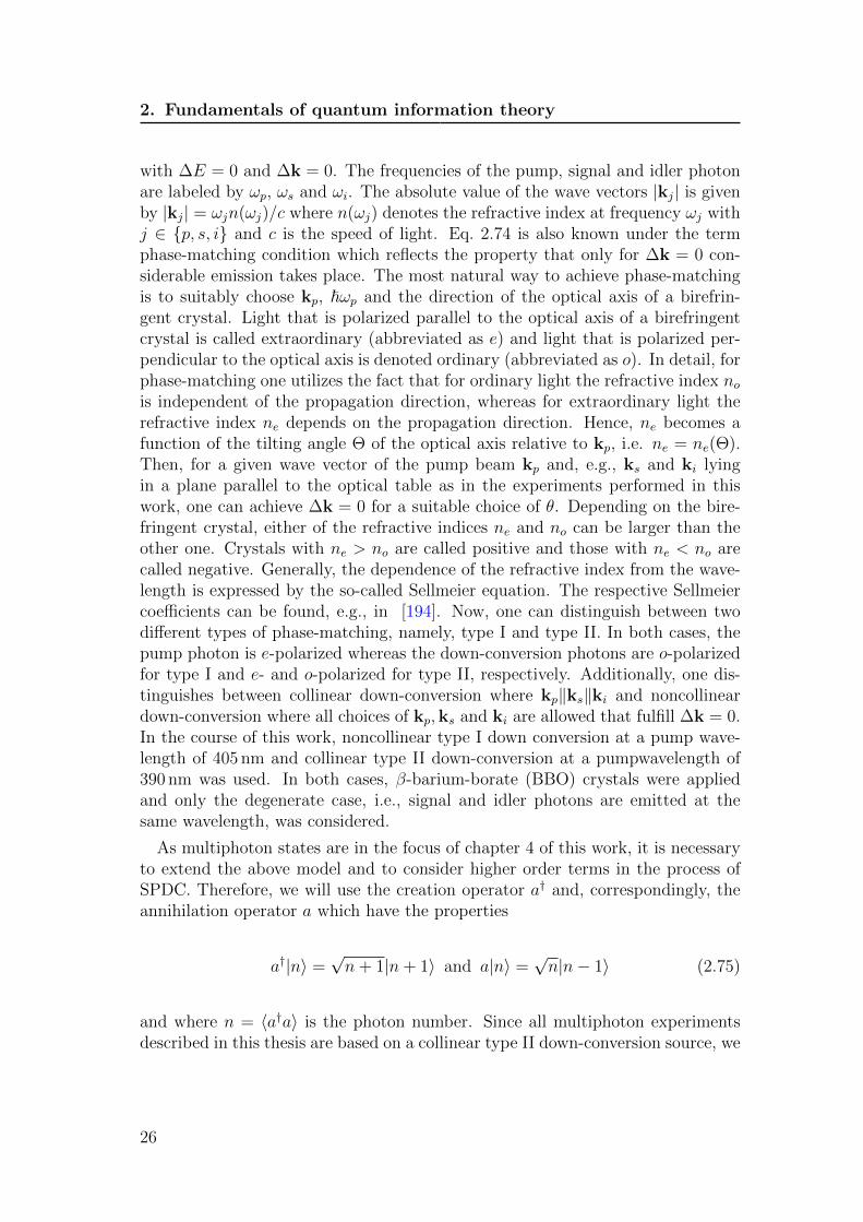
with ∆E = 0 and ∆k = 0. The frequencies of the pump, signal and idler photonare labeled by ωp, ωs and ωi. The absolute value of the wave vectors |kj| is givenby |kj| = ωjn(ωj)/c where n(ωj) denotes the refractive index at frequency ωj withj ∈ {p, s, i} and c is the speed of light. Eq. 2.74 is also known under the termphase-matching condition which reflects the property that only for ∆k = 0 con-siderable emission takes place. The most natural way to achieve phase-matchingis to suitably choose kp, ~ωp and the direction of the optical axis of a birefrin-gent crystal. Light that is polarized parallel to the optical axis of a birefringentcrystal is called extraordinary (abbreviated as e) and light that is polarized per-pendicular to the optical axis is denoted ordinary (abbreviated as o). In detail, forphase-matching one utilizes the fact that for ordinary light the refractive index nois independent of the propagation direction, whereas for extraordinary light therefractive index ne depends on the propagation direction. Hence, ne becomes afunction of the tilting angle Θ of the optical axis relative to kp, i.e. ne = ne(Θ).Then, for a given wave vector of the pump beam kp and, e.g., ks and ki lyingin a plane parallel to the optical table as in the experiments performed in thiswork, one can achieve ∆k = 0 for a suitable choice of θ. Depending on the bire-fringent crystal, either of the refractive indices ne and no can be larger than theother one. Crystals with ne > no are called positive and those with ne < no arecalled negative. Generally, the dependence of the refractive index from the wave-length is expressed by the so-called Sellmeier equation. The respective Sellmeiercoefficients can be found, e.g., in [194]. Now, one can distinguish between twodifferent types of phase-matching, namely, type I and type II. In both cases, thepump photon is e-polarized whereas the down-conversion photons are o-polarizedfor type I and e- and o-polarized for type II, respectively. Additionally, one dis-tinguishes between collinear down-conversion where kp‖ks‖ki and noncollineardown-conversion where all choices of kp,ks and ki are allowed that fulfill ∆k = 0.In the course of this work, noncollinear type I down conversion at a pump wave-length of 405 nm and collinear type II down-conversion at a pumpwavelength of390 nm was used. In both cases, β-barium-borate (BBO) crystals were appliedand only the degenerate case, i.e., signal and idler photons are emitted at thesame wavelength, was considered.
As multiphoton states are in the focus of chapter 4 of this work, it is necessaryto extend the above model and to consider higher order terms in the process ofSPDC. Therefore, we will use the creation operator a† and, correspondingly, theannihilation operator a which have the properties
a†|n〉 =√n+ 1|n+ 1〉 and a|n〉 =
√n|n− 1〉 (2.75)
and where n = 〈a†a〉 is the photon number. Since all multiphoton experimentsdescribed in this thesis are based on a collinear type II down-conversion source, we
26
2.3. Experimental realization of photonic multiqubit states
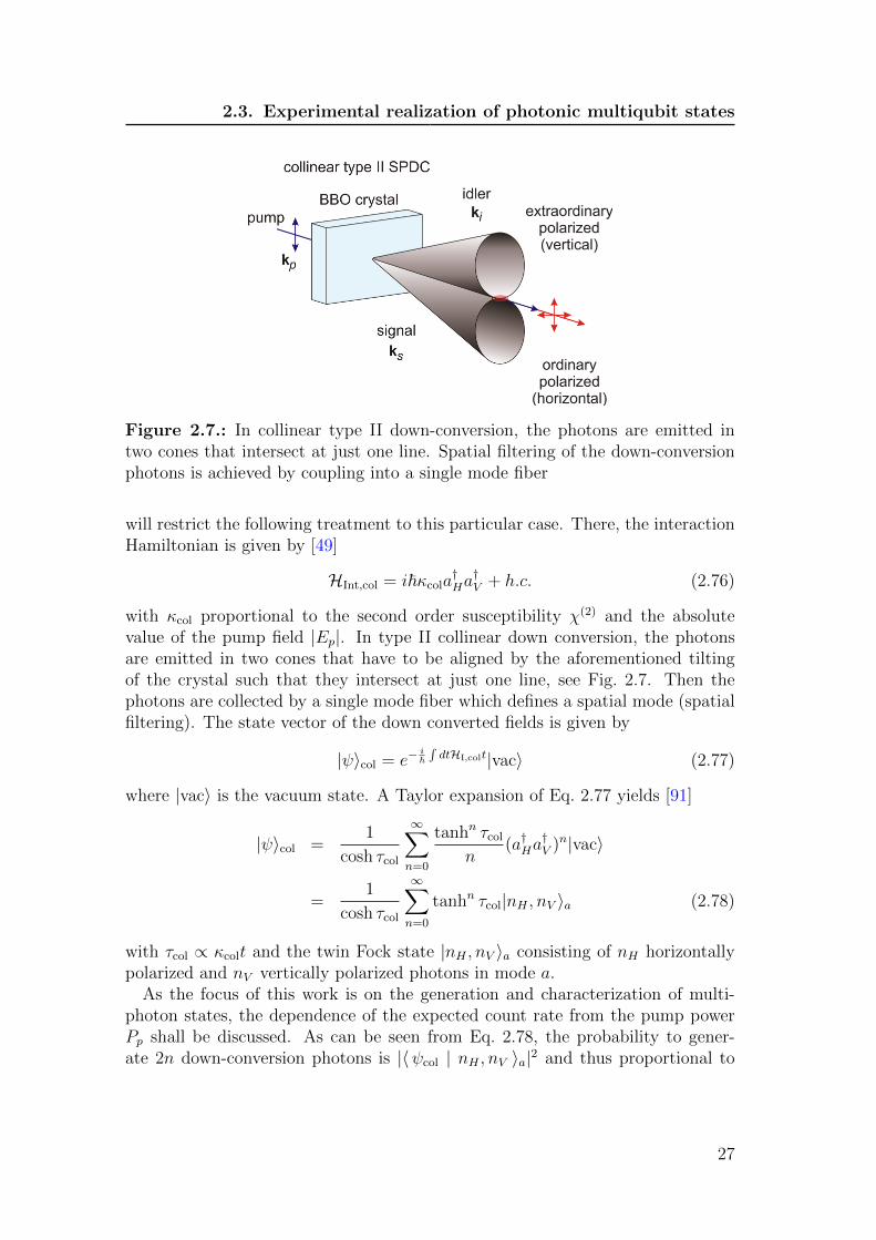
Figure 2.7.: In collinear type II down-conversion, the photons are emitted intwo cones that intersect at just one line. Spatial filtering of the down-conversionphotons is achieved by coupling into a single mode fiber
will restrict the following treatment to this particular case. There, the interactionHamiltonian is given by [49]
HInt,col = i~κcola†Ha†V + h.c. (2.76)
with κcol proportional to the second order susceptibility χ(2) and the absolutevalue of the pump field |Ep|. In type II collinear down conversion, the photonsare emitted in two cones that have to be aligned by the aforementioned tiltingof the crystal such that they intersect at just one line, see Fig. 2.7. Then thephotons are collected by a single mode fiber which defines a spatial mode (spatialfiltering). The state vector of the down converted fields is given by
|ψ〉col = e−i~∫dtHI,colt|vac〉 (2.77)
where |vac〉 is the vacuum state. A Taylor expansion of Eq. 2.77 yields [91]
|ψ〉col =1
cosh τcol
∞∑n=0
tanhn τcoln
(a†Ha†V )n|vac〉
=1
cosh τcol
∞∑n=0
tanhn τcol|nH , nV 〉a (2.78)
with τcol ∝ κcolt and the twin Fock state |nH , nV 〉a consisting of nH horizontallypolarized and nV vertically polarized photons in mode a.
As the focus of this work is on the generation and characterization of multi-photon states, the dependence of the expected count rate from the pump powerPp shall be discussed. As can be seen from Eq. 2.78, the probability to gener-ate 2n down-conversion photons is |〈ψcol | nH , nV 〉a|2 and thus proportional to
27

2. Fundamentals of quantum information theory
tanh2n τcol. Using the approximation tanh τcol ≈ τcol which is valid for τcol � 1one obtains the count rate is proportional to
τ 2ncol ∝ |Ep|2n ∝ P np . (2.79)
Hence, the count rates for the emission of n photon pairs increase polynomiallywith order n with the pump power. Nevertheless, due to the small nonlinearities ofcrystals like BBO, the likelihood to generate n photon pairs is very low. Thus, onehas to concentrate the pump power in short pulses which leads to a significantlyincreased creation probability per pulse.
Experimental implementation
As explained, in order to obtain reasonable count rates in multiphoton experi-ments based on SPDC, ultrashort laser pulses and high pump power are required.In the following, the photon source that was used for the experiments in publi-cations P3.3, P4.1 and P4.2 and which fulfills both these requirements shall bedescribed. More precisely, it will be discussed how SPDC photons are generatedthat are spatially, spectrally and temporarily indistinguishable, which is a prereq-uisite to use them for quantum information processing. A schematic drawing ofthe whole laser system including the SPDC source can be seen in Fig. 2.8. In a firststep, a continuous wave solid state laser at 1064 nm pumps a neodymium yttriumvanadate (Nd:YVO4) laser where up-conversion to 532 nm by second harmonicgeneration (SHG) takes place. The Nd:YVO4 is stabilized to lase at a constantoutput power of 10 W and is used to pump a titanium:sapphire (Ti:Sa) oscillator.The Ti:Sa oscillator delivers short pulses with a duration of approximately 130 fsat a repetition rate of 80 MHz. The center wavelength is 780 nm and the totaloutput power approximately 2W1. In the next step, up-conversion to 390 nm in a3 mm thick lithium-triborate (LBO) crystal is performed. The average power isapproximately 800 mW, but for multiphoton experiments with up to six photonsas performed in this work (see chapter 4), an even higher pump power is advan-tageous. Therefore, the light is coupled into an ultraviolet (UV) enhancementcavity [91, 195, 196] where a maximal UV pump power of up to 10 W can beachieved. For long-term stability of the cavity, two of its mirrors are mountedon piezo crystals, which allow for active stabilization using the Hansch-Couillaudlocking scheme [197]. Inside the bow-tie enhancement cavity, the light is focusedon a 1 mm thick anti-reflection coated BBO crystal that is cut for collinear type IIdown-conversion. One of the cavity mirrors has a dichroic coating with highreflectivity for the pump photons at 390 nm and high transmission for the down-conversion photons at 780 nm. It is known that due to the birefringence of the
1The three stages of the laser system are a TP80® power supply from Spectra Physics®, a10 W Millenia®XS from Spectra Physics®, and a Tsunami® Ti:Sa oscillator from SpectraPhysics®. The anti-reflection coated 1 mm thick BBO inside the cavity was obtained fromNewlight Photonics®.
28
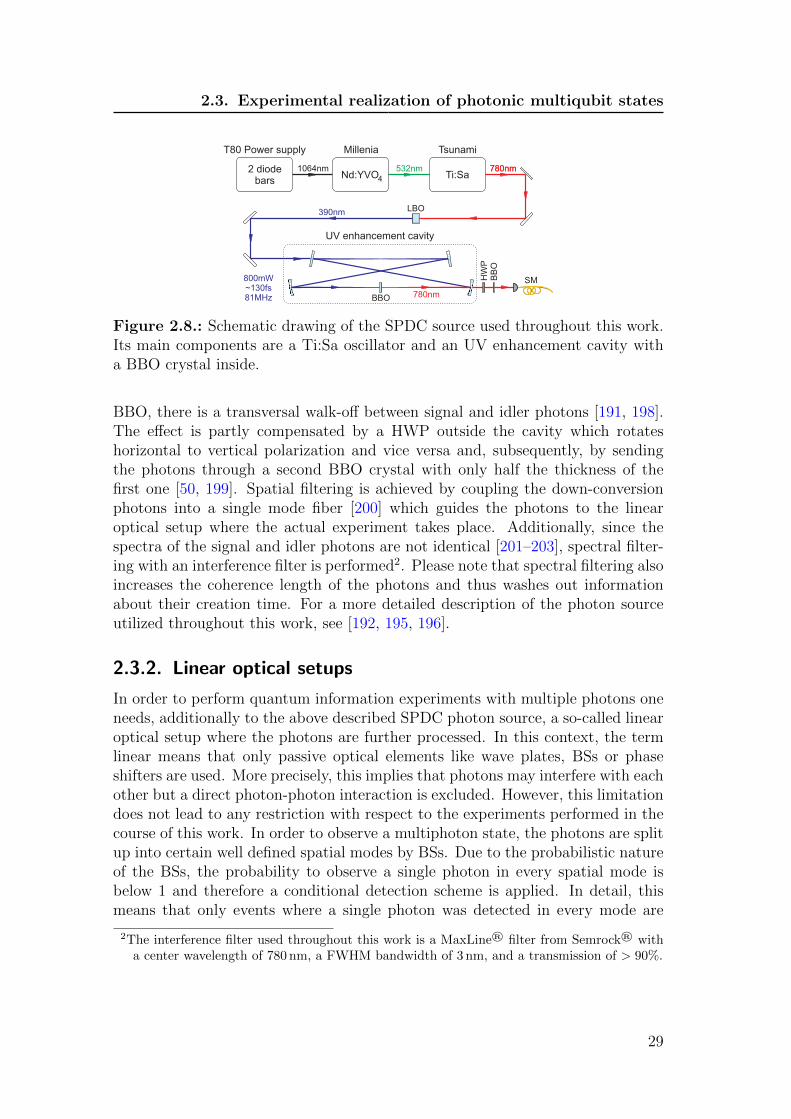
2.3. Experimental realization of photonic multiqubit states
Figure 2.8.: Schematic drawing of the SPDC source used throughout this work.Its main components are a Ti:Sa oscillator and an UV enhancement cavity witha BBO crystal inside.
BBO, there is a transversal walk-off between signal and idler photons [191, 198].The effect is partly compensated by a HWP outside the cavity which rotateshorizontal to vertical polarization and vice versa and, subsequently, by sendingthe photons through a second BBO crystal with only half the thickness of thefirst one [50, 199]. Spatial filtering is achieved by coupling the down-conversionphotons into a single mode fiber [200] which guides the photons to the linearoptical setup where the actual experiment takes place. Additionally, since thespectra of the signal and idler photons are not identical [201–203], spectral filter-ing with an interference filter is performed2. Please note that spectral filtering alsoincreases the coherence length of the photons and thus washes out informationabout their creation time. For a more detailed description of the photon sourceutilized throughout this work, see [192, 195, 196].
2.3.2. Linear optical setups
In order to perform quantum information experiments with multiple photons oneneeds, additionally to the above described SPDC photon source, a so-called linearoptical setup where the photons are further processed. In this context, the termlinear means that only passive optical elements like wave plates, BSs or phaseshifters are used. More precisely, this implies that photons may interfere with eachother but a direct photon-photon interaction is excluded. However, this limitationdoes not lead to any restriction with respect to the experiments performed in thecourse of this work. In order to observe a multiphoton state, the photons are splitup into certain well defined spatial modes by BSs. Due to the probabilistic natureof the BSs, the probability to observe a single photon in every spatial mode isbelow 1 and therefore a conditional detection scheme is applied. In detail, thismeans that only events where a single photon was detected in every mode are
2The interference filter used throughout this work is a MaxLine® filter from Semrock® witha center wavelength of 780 nm, a FWHM bandwidth of 3 nm, and a transmission of > 90%.
29
2. Fundamentals of quantum information theory
considered. Generally, every multiphoton experiment requires, depending on thestate one wants to prepare, a different linear optical setup and, therefore, only thebasic building blocks shall be discussed here. For the specific setups used for thisthesis, refer to chapters 3 and 4 and the corresponding publications at the end ofthese chapters.
Birefringent phase shifters
The simplest components of linear optical setups with only a single input and out-put mode are birefringent phase shifters. They perform unitary transformationslike, e.g., a rotation of the polarization or adding a phase between two orthogonalpolarizations. In photonic setups, the polarization is commonly manipulated withQWPs and HWPs. Such devices can be implemented with uniaxial birefringentcrystals like, e.g., quartz. Commonly, a wave plate consists of two crystals thatare cut parallel to their optical axis and then optically contacted (or cemented)with their optical axis crossed. Depending on the different thickness of the twocrystals, any phase shift can be implemented exactly, i.e., the phase shift is, e.g.,π/2 and not π/2 + 2nπ, n ∈ N. The main advantage of using two crystals in aconfiguration with n = 0, also known as zero-order configuration, is its reducedsensitivity with respect to shifts of the wavelength or temperature changes incomparison to a wave plate consisting of a single crystal only. For |z+〉 and |z−〉chosen as basis states and θ defined as the angle between the optical axis andthe |z+〉 direction, the corresponding transformations for a HWP and a QWP aregiven by [204]
HWP(θ) =
(cos 2θ sin 2θsin 2θ − cos 2θ
)= sin 2θσx + cos 2θσz (2.80)
QWP(θ) =
(cos2 θ − i sin2 θ (1 + i) cos θ sin θ
(1 + i) cos θ sin θ −i cos2 θ + sin2 θ
)=
1
2((1− i)1 + 2(1 + i) cos θ sin θσx + (1 + i) cos 2θσz). (2.81)
In general, an arbitrary unitary transformation cannot be realized with a singlewave plate. However, a combination of three wave plates, two QWPs and oneHWP allows for arbitrary unitary transformations. In particular, such a trans-formation is given by U(θ1, θ2, θ3) = QWP(θ1)HWP(θ2)QWP(θ3) with properlychosen angles θ1, θ2, and θ3. Please note that in order to realize a certain unitarytransformation, the choice of angles θ1, θ2 and θ3 is not unique and, in many cases,these angles can only be found numerically.
In some applications, like, e.g., the compensation of unwanted phase shifts asinduced by the Goos-Hanchen effect [205], it is necessary to shift a phase between|z+〉 and |z−〉. This can be realized by rotating a birefringent crystal with its
30

2.3. Experimental realization of photonic multiqubit states
optical axis parallel to |z−〉 around |z−〉 and thus varying the thickness of thecrystal. In particular, the transformation can be expressed as
PS(φ) =
(i cos φ
2+ sin φ
20
0 i cos φ2− sin φ
2
)= i cos
φ
21 + sin
φ
2σz (2.82)
where φ designates the angle by how much the crystal is rotated. Experimentally,yttrium-vanadate (YVO4) crystals are applied as phase shifter both as single crys-tals [191, 206] and in pairs with the optical axis of the crystals crossed [131, 207],analogously to the zero-order configuration common for wave plates.
Beam splitters
Beam splitters are four port devices with two input and two output ports andare used to split up or overlap spatial modes. They are characterized by theirreflectivity RH (RV ) and transmittance TH (TV ) for the respective polarization.For a lossless BS with real transmittance and reflectivity, RH + TH = 1 andRV + TV = 1 holds. With the corresponding input and output modes labeled asin Fig. 2.9a), the transformation of a BS can be expressed by means of creationand annihilation operators
a†H −→ 1√2
(√THc
†H + i
√RHd
†H) (2.83)
a†V −→ 1√2
(√TV c
†V + i
√RV d
†V ) (2.84)
b†H −→ 1√2
(√THd
†H + i
√RHc
†H) (2.85)
b†V −→ 1√2
(√TV d
†V + i
√RV c
†V ). (2.86)
Note that a BS introduces a phase shift of eiπ/2 which is required to guaranteeunitarity [208].
Projection measurements in arbitrary bases
In order to analyze quantum states, e.g., by means of state tomography as willbe discussed in chapter 4, it is necessary to perform projection measurements onvarious different basis states. However, experimentally, it is often only possibleto perform σz measurements, i.e, to project on |z+〉 and |z−〉. Therefore, thenatural question arises how a measurement in an arbitrary basis like σ(θ, φ) fromEq. 2.3 can be performed. More precisely, a general procedure has to be foundsuch that one can project on the eigenvectors |ψ(θ, φ)〉 and |ψ(θ, φ)〉⊥ of σ(θ, φ).
31

2. Fundamentals of quantum information theory
Figure 2.9.: The most important building blocks of linear optical setups area) BSs and b) polarization analyses. A BS is defined by the transformations itperforms on its input modes. A combination of a polarizing BS (PBS), i.e., a BSthat transmits horizontally polarized light and reflects vertically polarized light,and a HWP and QWP, as shown in b), can be used to separate photons with twoorthogonal eigenstates. Afterwards the photons are sent on APDs for detection.
The solution to this problem is to perform an appropriate unitary operation onthe state to be analyzed before the projection measurements. One possibility is tofirst apply a HWP(θ1), then a QWP(θ2) and finally measure σz with a polarizingBS, see Fig. 2.9b). The angles θ1 and θ2 have to be chosen such that the relations
QWP(θ2)HWP(θ1)|ψ(θ, φ)〉 = |z+〉 (2.87)
QWP(θ2)HWP(θ1)|ψ(θ, φ)〉⊥ = |z−〉 (2.88)
are fulfilled, or, equivalently,
σz = |z+〉〈z+| − |z−〉〈z−|= (QWP(θ2)HWP(θ1))σ(θ, φ)(QWP(θ2)HWP(θ1))
†. (2.89)
In many cases the angles θ1 and θ2 can only be determined numerically. However,for the most common basis settings, an analytic solution can be given as shownin Tab. 2.1.
Data acquisition
At every output of the polarization analysis, the photons are coupled into mul-timode fibers that are connected to actively quenched avalanche photo diodes3
(APD) which have a detection efficiency of 55% − 65% at 780 nm. The pho-ton counting modules are connected to a coincidence logic based on a field pro-grammable gate array (FPGA)4 [91], which allows for conditional detection. Thepulse rate of the laser is measured with a photo diode and fed into the external
3Throughout this work, photon counting modules SPCM-AQ4C from Perkin Elmer® wereused.
4The FPGA was a VirtexTM-4 XC4VLX25-FF668-10 produced by Xilinx®.
32

2.3. Experimental realization of photonic multiqubit states
measurement angle θ1 of HWP angle θ2 of QWPsetting
σx 22.5◦ 0σy 0 45◦
σz 0 0
Table 2.1.: In many experimental realizations, only measurements in the σz basiscan be directly carried out. Therefore, in order to perform measurements in otherbases, like σx or σy, one first has to apply a unitary transformation. One possibleimplementation is a combination of a HWP and QWP at appropriate angles θ1and θ2 in addition to a subsequent measurement in the σz basis.
clock of the FPGA. Consequently, the FPGA has a maximal detection rate ofup to 81 MHz. The FPGA is capable of processing the detection signals of 12photon counters which allows to perform multiphoton experiments with up to sixphotons. In order to carry out measurements in arbitrary bases, the HWP andQWP of every polarization analysis can be rotated with stepper motors5.
5All rotation stages are DRTM 40-D25-0SM440-(K) manufactured by OWIS®.
33

2. Fundamentals of quantum information theory
34

3. Entanglement detection bycorrelation measurements
In every experiment with entangled quantum states, it is crucial to first prove thatthe prepared states are actually entangled by means of suitable entanglement cri-teria (see section 2.2.3). In general, one can distinguish between entanglementcriteria that are state independent but often require complete knowledge of thedensity matrix and criteria that are state dependent like, e.g., entanglement wit-nesses and require only few measurements. Obviously, one would like to haveentanglement criteria at hand that are, at the same time, as general as possiblebut require only partial knowledge of the state.
In this chapter, such entanglement criteria will be presented. They are basedon correlation functions which are directly accessible in experiments and whichdo not require to determine the complete density matrix. The chapter is dividedinto two parts. In the first part, a simple entanglement criterion proposed byBadziag et al. [51] will be presented which is utilized to develop two schemes todetect entanglement at minimal experimental effort. The first scheme is based onSchmidt decomposition and requires at maximum three correlation measurementsto prove entanglement of pure two-qubit states. The second scheme is based onthe principle of correlation complementarity and allows to detect entanglementin an N -qubit state with an exponential speedup in comparison to random cor-relation measurements [53]. The description of these schemes stresses especiallyaspects that could not be discussed in publications P3.1 and P3.2.
As almost all entanglement criteria based on correlations rely on N -partite cor-relation functions [51, 60, 64–71], one might expect that the existence of N -partitecorrelations is a prerequisite for genuine N -partite entanglement. However, thisassumption turns out to be wrong, as first shown by Kaszlikowski et al. [74]. Inthe second part of this chapter, a general construction principle for N -partiteentangled states without N -partite correlations is presented. Interestingly, suchstates can even violate Bell inequalities which means, in consequence, that thereis no local realistic model describing their properties as shown in publication P3.3.
35

3. Entanglement detection by correlation measurements
3.1. Optimized state-independent entanglementdetection
In the following section, it will be discussed how correlations can be used as anefficient tool to detect entanglement. Therefore, at first, it is necessary to explainhow correlations are measured in practice. In section 2.2.1, it was explained thatevery quantum state % can be expressed by its correlations Ti1,i2,...,iN which canformally be determined as
Ti1,i2,...,iN = Tr[%σi1 ⊗ σi2 ⊗ ...⊗ σiN ] (3.1)
with i1, i2, ..., iN ∈ {0, x, y, z}. Experimentally, correlations are inferred from theexpectation values of projection measurements. Therefore, the Pauli matrices inEq. 3.1 are expressed in their eigenbases, i.e.,
σ0 = |x+ 〉〈x+ | + |x− 〉〈x− |= |y+ 〉〈 y+ | + |y− 〉〈 y− |= |z+ 〉〈 z+ | + |z− 〉〈 z− | (3.2)
σx = |x+ 〉〈x+ | − |x− 〉〈x− | (3.3)
σy = |y+ 〉〈 y+ | − |y− 〉〈 y− | (3.4)
σz = |z+ 〉〈 z+ | − |z− 〉〈 z− | . (3.5)
For example, the correlation Tz,z of a two-qubit state, can then be inferred fromthe following projection measurements
Tz,z = Tr[%(σz ⊗ σz)]= Tr
[%(|z+ 〉〈 z+ | − |z− 〉〈 z− |)⊗ (|z+ 〉〈 z+ | − |z− 〉〈 z− |)
]= Tr
[% |z+ 〉〈 z+ | ⊗ |z+ 〉〈 z+ |
]− Tr
[% |z+ 〉〈 z+ | ⊗ |z− 〉〈 z− |
]− Tr
[% |z− 〉〈 z− | ⊗ |z+ 〉〈 z+ |
]+ Tr
[% |z− 〉〈 z− | ⊗ |z− 〉〈 z− |
]. (3.6)
All other correlations can be determined correspondingly.
3.1.1. Experimentally friendly entanglement criterion
The entanglement criterion used throughout this chapter was originally proposedby Badziag et al. [51] and originates from the following geometrical observation.Consider two real unit vectors ~s and ~e together with their scalar product: If therelation ~s · ~e < ~e · ~e holds, then the two vectors cannot be identical, i.e., ~s 6= ~e.In a few steps, this simple geometrical fact will be transformed into a practicalentanglement criterion [51]. For this purpose, a scalar product (·, ·) for correlationtensors has to be introduced
(T %A , T %B) =∑
i1,...,iN∈{0,x,y,z}
T %Ai1,...,iNT%Bi1,...,iN
(3.7)
36
3.1. Optimized state-independent entanglement detection
where T %A and T %B are the correlation tensors of two states %A and %B. Asexplained in chapter 2, a state %sep is fully separable if it can be written as aconvex sum of the form
%sep =∑i
pi(%1)i ⊗ ...⊗ (%N)i (3.8)
with pi > 0 and∑i
pi = 1. For such states also the correlation tensor T %sep becomes
separable
T %sep =∑i
piTprodi with T prod
i = T(1)i · T
(2)i · ... · T
(N)i (3.9)
and where the T(k)i (k = 1, ..., N) describe single-qubit correlation tensors. Com-
bining the geometrical observation mentioned above with Eq. 3.7 and Eq. 3.9, oneobtains the following entanglement criterion:
If a state % with correlation tensor T % is fully separable, then there must be apure product state associated with the correlation tensor T prod such that the in-equality (T %, T prod) ≥ (T %, T %) holds.
The validity of this inequality can easily be proven by assuming that the con-trary is true, i.e., (T %, T prod) < (T %, T %). This would imply, due to the separabilityof T %, that
(T %, T %) =∑i
pi(T%, T prod
i ) <∑i
pi(T%, T %) = (T %, T %) (3.10)
which is a contradiction. Hence, if the inequality
maxTprod
(T %, T prod) < (T %, T %) (3.11)
is true, % must be entangled. If one now restricts the indices i1, ..., iN in Eq. 3.7to {x, y, z}, i.e.,
(T %A , T %B) =∑
i1,...,iN∈{x,y,z}
T %Ai1,...,iNT%Bi1,...,iN
, (3.12)
the maximal attainable value of the left-hand side of Eq. 3.11 is given by [51]
Tmax = max~m1⊗...⊗~mN
(T %, ~m1 ⊗ ...⊗ ~mN) (3.13)
where the ~mk = (T(k)x , T
(k)y , T
(k)z ) are unit vectors and can be associated with a
pure state of the kth party. More precisely, Tmax corresponds to the expectationvalue of a correlation measurement, where σ(k) = T
(k)x σx+T
(k)y σy+T
(k)z σz is chosen
as the local measurement basis for the kth qubit. Since the absolute value of a
37

3. Entanglement detection by correlation measurements
correlation can be 1 at maximum, this finally results in the desired entanglementcriterion: A quantum state % is entangled if∑
i1,...,iN∈{x,y,z}
(T %i1,...,iN )2 > 1 (3.14)
holds. From the experimental point of view, this is a remarkably positive resultbecause it means that one can start measuring correlations according to Eq. 3.14and, as soon as the threshold of Eq. 3.14 is surpassed, entanglement is detectedand one can stop measuring. The challenge now is to find strategies that allow tobreak the threshold with as little experimental effort as possible.
3.1.2. Experimental Schmidt decomposition
The first strategy to surpass the limit of 1 in Eq. 3.14 is tailored to pure or closeto pure two-qubit states and is based on a redefinition of the local measurementdirections. Every pure two-qubit state can be expressed in a particular form [62,209]
|ψS〉 = cos θ|a〉|b〉+ sin θ|a⊥〉|b⊥〉 θ ∈ [0, π/4] (3.15)
called Schmidt decomposition with local bases |a〉/|a⊥〉 and |b〉/|b⊥〉. The localbases are denoted as Schmidt bases and allow both parties to define their re-spective local measurements. For the first party, from now on called Alice, oneobtains
σx′ = |a⊥〉〈a|+ |a〉〈a⊥|σy′ = i|a⊥〉〈a| − i|a〉〈a⊥|σz′ = |a〉〈a| − |a⊥〉〈a⊥| (3.16)
with corresponding definitions of σx′′ , σy′′ and σz′′ for the second party calledBob. The main advantage of the Schmidt decomposition with respect to fastentanglement detection is that it leads to a “concentration” of the correlations.More precisely, it results in a diagonalization of the correlation tensor which canbe interpreted as a 4 × 4 matrix in the two-qubit case, see Fig. 3.1. Then, theentanglement criterion Eq. 3.14 allows to detect entanglement of all entangled puretwo-qubit states (i.e. θ 6= 0) from measuring Tz′,z′′ and Ty′,y′′ since T 2
z′,z′′+T 2y′,y′′ =
1+T 2y′,y′′ > 1. However, generally, the computational basis does not coincide with
the Schmidt basis and, therefore, a simple procedure to determine the Schmidtbasis is required. In order to find such a procedure, in a first step, the basis vectorsof the respective Schmidt bases are expressed in terms of the computational basis
|a〉 = cos ξA|0〉+ eiϕA sin ξA|1〉|a⊥〉 = sin ξA|0〉 − eiϕA cos ξA|1〉|b〉 = cos ξB|0〉+ eiϕB sin ξB|1〉|b⊥〉 = eiδ(cos ξB|0〉 − eiϕB cos ξB|1〉). (3.17)
38
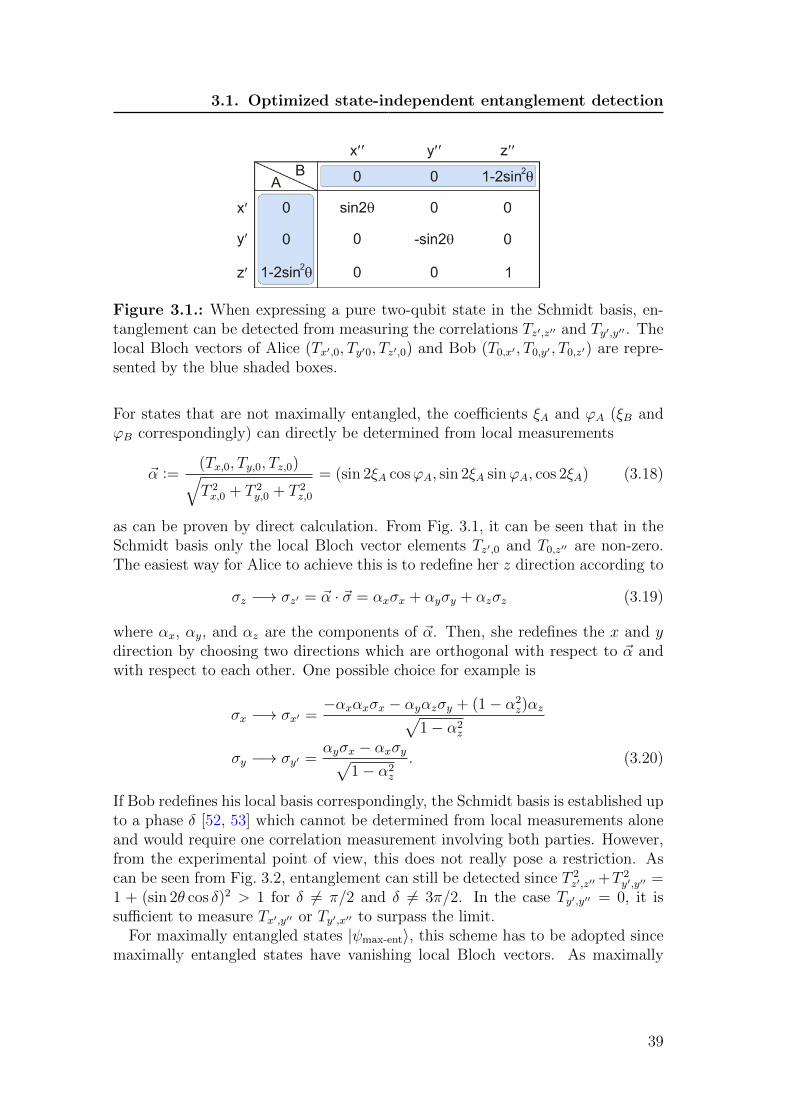
3.1. Optimized state-independent entanglement detection
Figure 3.1.: When expressing a pure two-qubit state in the Schmidt basis, en-tanglement can be detected from measuring the correlations Tz′,z′′ and Ty′,y′′ . Thelocal Bloch vectors of Alice (Tx′,0, Ty′0, Tz′,0) and Bob (T0,x′ , T0,y′ , T0,z′) are repre-sented by the blue shaded boxes.
For states that are not maximally entangled, the coefficients ξA and ϕA (ξB andϕB correspondingly) can directly be determined from local measurements
~α :=(Tx,0, Ty,0, Tz,0)√T 2x,0 + T 2
y,0 + T 2z,0
= (sin 2ξA cosϕA, sin 2ξA sinϕA, cos 2ξA) (3.18)
as can be proven by direct calculation. From Fig. 3.1, it can be seen that in theSchmidt basis only the local Bloch vector elements Tz′,0 and T0,z′′ are non-zero.The easiest way for Alice to achieve this is to redefine her z direction according to
σz −→ σz′ = ~α · ~σ = αxσx + αyσy + αzσz (3.19)
where αx, αy, and αz are the components of ~α. Then, she redefines the x and ydirection by choosing two directions which are orthogonal with respect to ~α andwith respect to each other. One possible choice for example is
σx −→ σx′ =−αxαxσx − αyαzσy + (1− α2
z)αz√1− α2
z
σy −→ σy′ =αyσx − αxσy√
1− α2z
. (3.20)
If Bob redefines his local basis correspondingly, the Schmidt basis is established upto a phase δ [52, 53] which cannot be determined from local measurements aloneand would require one correlation measurement involving both parties. However,from the experimental point of view, this does not really pose a restriction. Ascan be seen from Fig. 3.2, entanglement can still be detected since T 2
z′,z′′+T 2y′,y′′ =
1 + (sin 2θ cos δ)2 > 1 for δ 6= π/2 and δ 6= 3π/2. In the case Ty′,y′′ = 0, it issufficient to measure Tx′,y′′ or Ty′,x′′ to surpass the limit.
For maximally entangled states |ψmax-ent〉, this scheme has to be adopted sincemaximally entangled states have vanishing local Bloch vectors. As maximally
39

3. Entanglement detection by correlation measurements
Figure 3.2.: When only local measurement are performed by Alice and Bob,their local Schmidt bases can only be determined up to a relative phase δ. Thelocal Bloch vectors of Alice and Bob are represented by the blue shaded boxes.
entangled states admit infinity many Bloch decompositions [67], one of the twoparties, like, e.g. Bob, can therefore freely chose a local coordinate system. Let usassume that he decides to stick with his basis definition. Then Bob implies a filteroperation of the form F = |0〉〈0| + ε|1〉〈1| (0 < ε < 1) which, if it is successful1,results in a state that is not maximally entangled
(1⊗ F )|ψmax-ent〉 =1√
1 + ε2(|a〉|0〉+ ε|a⊥〉|1〉) (3.21)
and thus leads to an emerging local Bloch vector with Alice. Hence, Alice can re-define her local measurement directions according to Eq. 3.19 and Eq. 3.20. AfterBob removes the filter, entanglement can again be detected by measuring Tz′,z′′and Ty′,y′′ . Please note that the filter operation can also be seen as a test which al-lows to distinguish between maximally entangled states and the maximally mixedstate because for the maximally mixed state, the local Bloch vectors would notemerge after filtering.
In summary, the presented scheme allows to detect entanglement of all pure en-tangled states with six local measurements, if necessary, filtering by Bob togetherwith Alice measuring her local Bloch vector a second time, and, at most, threecorrelation measurements. For more details concerning the performance and anexperimental implementation of the scheme, see P3.1 and P3.2.
3.1.3. Decision tree
The second strategy to break the threshold of Eq. 3.14 is based on the principleof correlation complementarity [60, 63]. The term correlation complementaritydenotes the fact that for a set of dichotomic, mutually anticommuting operators{σ1, σ2, ..., σN} the trade-off relation
T 2σ1
+ T 2σ2
+ ...+ T 2σN≤ 1 (3.22)
1Since Bob has to inform Alice whether the filtering operation was successful or not, thismeasurement is not local.
40

3.1. Optimized state-independent entanglement detection
holds where Tσk (k = 1, ..., N) is the expectation value of σk. Consequently, thismeans that as soon as one of the expectation values is extremal, i.e., Tσj = ±1,then all Tσk with k 6= j have to vanish. As only non-zero correlations contribute tothe criterion of Eq. 3.14, the vanishing correlations do not have to be determined.Hence, correlation complementarity can be used to design a measurement schemethat reduces the experimental effort considerable.
In the two-qubit case, such a scheme can be given in a compact form, called de-cision tree. Alice and Bob chose independently from each other three orthogonaldirections and agree to measure correlations along these directions. For simplicity,the measurement directions are abbreviated as x, y, z for both Alice and Bob. The
Figure 3.3.: The decision tree for fast entanglement detection of two qubits.Alice and Bob chose their local measurement directions independently from eachother and agree to perform correlation measurements along these directions, i.e.,no shared reference frame is required. The tree starts with a measurement of Tz,zand for each following step one proceeds along the continuous arrow if the absolutevalue of the correlation measurement is > 0.4. The scheme succeeds as soon as∑
i,j∈{x,y,z} T2i,j > 1. Every maximally entangled pure state with its Schmidt bases
aligned along x,y, or z is detected as entangled within the blue shaded area.
sequence of the correlation measurements is given by the decision tree in Fig. 3.3and the results of the corresponding measurements. It starts with a measure-ment of Tz,z and continues along the continuous arrow if |Tz,z| > 0.4 and alongthe dashed one otherwise. At every following step, one measures the respectivecorrelation and proceeds along the continuous or the dashed arrow depending onwhether the absolute value of the result is above or below 0.4. The scheme ends
41

3. Entanglement detection by correlation measurements
as soon as entanglement is detected, i.e., as soon as∑
i,j∈{x,y,z} T2i,j > 1. The op-
timal value for the decision parameter was determined by numerical simulationsshowing that the best choice is 0.4.
In order to evaluate the performance of the decision tree, it has to be comparedagainst randomly chosen correlation measurements. As random sampling, in con-
Figure 3.4.: Efficiency of the two-qubit decision for randomly mixed states ac-cording to the Haar measure. The efficiency of the tree in comparison with randommeasurements increases both with a) the purity of the state as well as with b) theentanglement as quantified by the negativity.
trast to the decision tree, does not take into account correlation complementarity,one expects a better performance for the tree. That this is actually the case canbe seen in Fig. 3.4a) where the number of states detected by the decision tree iscompared against random sampling for different purities. As expected, all pureentangled states are detected by both the tree and random sampling, however, thetree succeeds faster. The advantage of the tree is more pronounced for pure states.A similar behavior is observed for the negativity as shown in Fig. 3.4b). All stateswith a negativity > 0.2 are detected as entangled and the tree succeeds fasterthan random measurements. For more details on the performance of the decisiontree and how it can be generalized to more than two qubits, see publication P3.2.
3.2. No correlation states
In this part, a particular class of states will be discussed which has vanishingN -partite correlations but still exhibits N -partite entanglement. The first memberstate of this class was discussed by Kaszlikowski et al. [74]. Here, the result ofKaszlikowski will be generalized and a constructive scheme that allows to constructsuch particular states will be given. Therefore, at first the concept of antistateshas to be introduced, and second, the entanglement criterion of Eq. 3.11 has tobe adopted such that genuine N -partite entanglement for vanishing N -partitecorrelations can be detected.
42

3.2. No correlation states
3.2.1. States and antistates
For every pure state |ψ〉 with an odd number of qubits, there exists an antistate|ψ〉, such that, by evenly mixing |ψ〉 and |ψ〉
%ncψ =1
2|ψ 〉〈ψ | +1
2|ψ 〉〈ψ | (3.23)
all N -partite correlations of %ncψ vanish. In detail, the antistate has reversed cor-relations with respect to |ψ〉 for every odd number of parties whereas all othercorrelations are unchanged. In order to find the antistate, let us first consider |ψ〉expressed in the computational basis
|ψ〉 =1∑
k1,...,kN=0
αk1,...,kN |k1, ..., kN〉 (3.24)
with normalized coefficients αk1,...,kN ∈ C. Mathematically, |ψ〉 can be obtainedby applying local universal-not gates [210] GUNOT = (σzσxK) with K denotingcomplex conjugation in the computational basis. Direct calculation shows thatGUNOTσxG
†UNOT = −σx, GUNOTσyG
†UNOT = −σy and GUNOTσzG
†UNOT = −σz and
thus only correlations for an odd number of observers are inverted. Applicationof GUNOT to all the subsystems yields
|ψ〉 =1∑
k1,...,kN=0
(−1)k1+...+kNα∗1−k1,...,1−kN |k1, ..., kN〉 (3.25)
where the asterisk∗ stands for complex conjugation. Please note that althoughGUNOT is an antiunitary operation, i.e., G†UNOT = −GUNOT, the antistate |ψ〉is always a well-defined quantum mechanical state. This construction principlecan easily be generalized to mixed states by defining % = G⊗NUNOT%(G⊗NUNOT)† whichtransforms every pure state in the decomposition of % into its antistate. For stateswith all αk1,...,kN ∈ R, complex conjugation is unnecessary and no-correlation statescan be obtained by local operations alone.
One might now wonder if a similar construction principle exists also for stateswith an even number of qubits. Interestingly, the answer turns out to be negativeas there is a counterexample where it can be shown that an antistate cannotexist. Let us consider the N -qubit GHZ state |GHZN〉 = 1/
√2(|0〉⊗N + |1〉⊗N)
with 2N−1 nonvanishing full correlations in the xy plane, non-zero Tz,...,z, and2N−1 − 1 nonvanishing correlations between a smaller number of subsystems. Allthese correlations have absolute value 1. Let us now assume that the GHZ statehas an antistate |GHZN〉 with inverted correlations between all N parties (withno constraints applied on correlations for a smaller number of parties). Then, the
43

3. Entanglement detection by correlation measurements
fidelity between the GHZ state and its antistate, expressed by the corresponding
correlation tensors TGHZNi1,...,iN
and TGHZNi1,...,iN
F = |〈GHZN | GHZN 〉|2 =1
2N
∑i1,...,iN∈{0,x,y,z}
TGHZNi1,...,iN
TGHZNi1,...,iN
< 0 (3.26)
is negative because more than half of the correlations have opposite sign. Hence,for GHZ states with an even number of qubits, there are no antistates. Thusa general construction principle to generate antistates with an even number ofqubits cannot exist.
3.2.2. Family of genuine entangled no correlation states
In this section, a whole family of entangled three-qubit states with vanishingtripartite correlations will be presented. As a starting point, let us consider thethree-qubit pure state
|φ(α, β)〉 = sin β cosα|001〉+ sin β sinα|010〉+ cos β|100〉 (3.27)
with α, β ∈ (0, π/2). Note that |φ(α, β)〉 (with any local unitaries applied thereon)defines a whole subspace of tripartite entangled states within the three-qubitHilbert space. Mixing |φ〉 with its antistate
|φ(α, β)〉 = sin β cosα|110〉+ sin β sinα|101〉+ cos β|011〉 (3.28)
defines a family of no-correlation states
%ncφ (α, β) = 0.5 |φ(α, β) 〉〈φ(α, β) | +0.5 |φ(α, β) 〉〈φ(α, β) | . (3.29)
In the following, it will be shown that, despite of vanishing tripartite correla-tions, all member states of the family %ncφ (α, β) are genuinely tripartite entangled.Therefore, the entanglement criterion of Eq. 3.11 is adopted to
maxTbi-sep
(T %, T bi-sep) < (T %, T %) (3.30)
where optimization is performed over all biseparable pure states %bi-sep. If inequal-ity 3.30 holds, then % cannot be biseparable, i.e., it must be genuinely tripartiteentangled. Please note that here the scalar product for correlations tensors as de-fined in Eq. 3.7 is used. As can be shown by direct calculation, the right-hand sideof Eq. 3.30 is 4 for all member states %ncφ (α, β) of the family [54]. Hence, in orderto decide for which values of α and β, the state %ncφ (α, β) is genuinely tripartiteentangled, the left-hand side of Eq. 3.30 has to be determined by performing anoptimization over all biseparable states. Since the optimization process is rather
44

3.2. No correlation states
3.4
3.5
3.6
3.7
3.8
3.9
1/8 π
1/4 π
3/8 π
1/2 π
α
00
1/8 π 1/4 π 3/8 π 1/2 π
β
Figure 3.5.: Contour plot of the left-hand side of the entanglement criterionof Eq. 3.30 for states of the family %ncφ (α, β). If the value is below 4, the stateis genuinely tripartite entangled. As can be seen, all states of the family withα, β 6= 0 and α, β 6= π/2 are entangled.
cumbersome, only the result is shown in Fig. 3.5 (for details please refer to theappendix of publication P3.3). As can be seen, the left-hand side of Eq. 3.30 isbelow 4 for all values of α, β 6= 0 and α, β 6= π/2 (which were excluded in thedefinition of |φ〉 anyway). Hence, the entire family of states %ncφ as defined inEq. 3.29 is genuinely tripartite entangled although, by definition, it has vanishingtripartite correlations.
As an example state of the family %ncφ , a mixture of the tree-qubit W state
(obtained by setting α = π/3 and β = cos−1(1/√
3)) with its antistate wasconsidered, i.e.,
%ncW = 0.5 |W 〉〈W | +0.5 |W 〉〈W | . (3.31)
Experimentally, such a state can be prepared by means of a four-photon symmetricDicke state |D(2)
4 〉 . As described by Wieczorek et al. [127], symmetric Dickestates can be used as a resource to prepare other entangled states by appropriateprojection measurements. The W state for example can be obtained from a |D(2)
4 〉state by projection of one qubit on |1〉. Correspondingly, the state W can beobtained from projection on |0〉. The target state %ncW can then be generated byevenly mixing the states W and W which is in practice realized by tracing outthe respective qubit. For details on the experimental implementation including adescription of the utilized optical setup, see publication P3.3.
At this point one might ask if a vanishing correlation does also mean thatone cannot infer another party’s measurement result from one’s own result. In
45

3. Entanglement detection by correlation measurements
Figure 3.6.: Observed detection frequencies of the states |W 〉exp (red) and |W 〉exp(blue) and %nc,expW (red and blue) when measuring in the σ⊗3z basis. The gray barsrepresent the theoretically expected values. From the detection frequencies, onecan infer the correlation value Tz,z,z for the respective states. Although Tz,z,zvanishes for the state %nc,expW , from one’s own, measurement result, one can stillmake predictions about the other parties outcomes with better success probabilitythan for pure guessing due to nonvanishing two-party correlations, like, e.g., Tz,z,0.
order to answer this question, let us consider Fig. 3.6 which displays the relativefrequencies that were measured in order to determine the correlation Tz,z,z =〈σz ⊗ σz ⊗ σz〉 of the experimentally prepared states |W〉, |W〉, and %ncW. Fordetails see publication P3.3. Please note that the computational basis |0〉 and |1〉used so far was encoded in the polarization degree of freedom of single photonsas |0〉 −→ |H〉 and |1〉 −→ |V〉 where H stands for horizontal and V for verticalpolarization. Commonly, horizontal polarization is associated with a parity of +1and for vertical polarization one has a parity of −1.
At first, one observes that the experimentally determined values of Tz,z,z for|W〉 and |W〉 are close to the theoretically expected values of −1 and 1 and thatby mixing the two states, Tz,z,z becomes zero. Also the experimentally determinedbipartite correlations T0,z,z, Tz,0,z, and Tz,z,0 are in good agreement with their the-oretical values of −1/3. With these correlations, one can make predictions basedon the parity of the measurement results of one or two parties. Let us thereforeconsider the W state that is shared between three parties. Since the value ofTz,z,z is −1, it follows that if the first two parties measure the same polarization,the third party has to measure vertical polarization. In case the first two par-ties measure orthogonal polarization, the third party has to measure horizontalpolarization. Similarly, from the bipartite correlations one can conclude that two
46

3.2. No correlation states
parties will measure the same polarization with probability 1/3 and orthogonalpolarization wit probability 2/3. Hence, for the state |W〉 and correspondinglyfor |W〉, from the parity of the measurement results of one or two parties, one canmake predictions about the third party’s outcome with better success probabilitythan pure guessing.
Interestingly, similar statements can also be made for the state %ncW. The ex-perimental value of Tz,z,z is close to the theoretical value of 0. The bipartitecorrelations T0,z,z, Tz,0,z, and Tz,z,0 are also in good agreement with their expectedvalues of −1/3. In contrast to the states |W〉 and |W〉, here, due to the van-ishing correlation Tz,z,z, it is not possible to infer the third party’s measurementresult from the product of the parities of the first two parties. However, from thebipartite correlations one can still infer that two parties will measure the samepolarization with probability 1/3 and orthogonal polarization wit probability 2/3.In summary, although the correlation Tz,z,z vanishes for the state %ncW, one can,based on the bipartite correlations T0,z,z, Tz,0,z, and Tz,z,0, still make predictionswith a success probability higher than for pure guessing.
As a closing remark to this section, it seems appropriate to shortly commenton the term correlation. In response to the paper by Kaszlikowski et al. [74], avivid discussion on a proper definition of classical and quantum correlations set in.Bennet et al. [75], for example, proposed a set of postulates that every measureof genuine multipartite correlations should fulfill:
Postulate 1 : If an N -partite state does not have genuine N -partite correla-tions and on adds a party in a product state, then the resulting N+1-partitestate does not have genuine N -partite correlations.
Postulate 2 : If an N -partite state does not have genuine N -partite corre-lations, then local operations and unanimous postselection (which mathe-matically corresponds to the operation Λ1 ⊗ Λ2 ⊗ ... ⊗ ΛN , where N is thenumber of parties and each Λi is a trace nonincreasing operation acting onthe ith party’s subsystem) cannot generate genuine N -partite correlations.
Postulate 3 : If an N -partite state does not have genuine N -partite corre-lations, then if one party splits his subsystem into two parts, keeping onepart for himself and using the other to create a new N + 1-st subsystem,then the resulting N + 1-partite state does not have genuine N + 1-partitecorrelations.
According to these postulates, the correlation function as defined in Eq. 2.41cannot be called a measure of genuine N -partite correlations as can be directlyshown. Let us therefore consider the N -qubit state |00...0〉 which has a vanishingTx,x,...,x correlation, i.e., Tx,x,...,x = Tr[| 00...0 〉〈 00...0 | σx ⊗ σx ⊗ ... ⊗ σx] = 0.However, by applying the local unitary transformation U = HWP(22.5◦)⊗N onthe state one obtains Tx,x,...,x = Tr[U | 00...0 〉〈 00...0 | U †σx ⊗ σx ⊗ ... ⊗ σx] = 1
47

3. Entanglement detection by correlation measurements
which is a violation of postulate 2. Hence, Tx,x,...,x and correspondingly all othercorrelations as defined in Eq. 2.41 cannot be a measure of genuine N -partitecorrelation according to the above postulates2. Interestingly, Bennet et al. couldnot find a measure satisfying all their postulates.
In another approach, Giorgi et al. [76] used an information-theoretic definition ofmultipartite correlations. According to their definition, genuine classical tripartitecorrelations of 0.813 bit and tripartite genuine quantum tripartite correlations of0.439 bit are assigned to the state %ncW. However, also the measure by Giorgi etal. does not fulfill all postulates by Bennet et al. At the time of writing, it isstill an open question whether a rigorous and easy to calculate measure of genuinecorrelations which is based on plausible postulates can be given.
3.3. Publications
2Please note that correlations according to Eq. 2.41 cannot be a measure at all as they canincrease under local unitary operations.
48
Experimental Schmidt Decomposition and State Independent Entanglement Detection
Wiesław Laskowski,1,2,3 Daniel Richart,2,3 Christian Schwemmer,2,3 Tomasz Paterek,4 and Harald Weinfurter2,3
1Institute of Theoretical Physics and Astrophysics, University of Gdansk, PL-80-952 Gdansk, Poland2Max-Planck-Institut fur Quantenoptik, Hans-Kopfermann-Strasse 1, D-85748 Garching, Germany
3Department fur Physik, Ludwig-Maximilians-Universitat, D-80797 Munchen, Germany4Centre for Quantum Technologies, National University of Singapore, 3 Science Drive 2, 117543 Singapore, Singapore
(Received 17 November 2011; revised manuscript received 6 April 2012; published 11 June 2012)
We introduce an experimental procedure for the detection of quantum entanglement of an unknown
quantum state with a small number of measurements. The method requires neither a priori knowledge of
the state nor a shared reference frame between the observers and can thus be regarded as a perfectly state-
independent entanglement witness. The scheme starts with local measurements, possibly supplemented
with suitable filtering, which essentially establishes the Schmidt decomposition for pure states.
Alternatively we develop a decision tree that reveals entanglement within few steps. These methods
are illustrated and verified experimentally for various entangled states of two and three qubits.
DOI: 10.1103/PhysRevLett.108.240501 PACS numbers: 03.67.Mn, 03.65.Ta, 03.67.Bg, 42.50.Ex
Introduction.—Entanglement is the distinguishing fea-ture of quantum mechanics and it is the most importantresource for quantum information processing [1,2]. Forany experiment it is thus of utmost importance to easilyreveal entanglement, ideally with as little effort aspossible. Common methods suffer from disadvantages.On the one hand, employing the Peres–Horodecki cri-terion [3,4] or evaluating entanglement measures, onecan identify entanglement in arbitrary states; however,it requires full state tomography. On the other hand,various entanglement witnesses [4–10] can be deter-mined with much fewer measurements, but they giveconclusive answers only if the state under investigationis close to the witness state; i.e., they require a prioriknowledge.
Recently, it has been shown that the existence of entan-glement can be inferred from analyzing correlations amongthe measurement results on the subsystems of a quantumstate. The properly weighted sum of correlations will over-come characteristic thresholds only if the state is entangled[11]. Here we further develop this approach to obtain asimple and practical method to detect entanglement of allpure states and some mixed states by measuring only asmall number of correlations. Since the method is adaptive,it does not require a priori knowledge of the state nor ashared reference frame between the possibly remote ob-servers, and thus it greatly simplifies the practical applica-tion. We describe two schemes. The first one essentiallycan be seen as a direct implementation of Schmidt decom-position, which identifies the maximal correlation directly.For bipartite pure systems, this approach can be dividedconceptually into two stages: (i) calibration that establishesthe experimental Schmidt decomposition [12,13] of a purestate by local measurements and suitable filtering and(ii) two correlation measurements to verify the entangle-ment criterion. The second scheme shows how to use a
decision tree to obtain a rapid violation of the threshold,thereby identifying entanglement.Entanglement criterion.—For a two-qubit quantum state
�, Alice and Bob observe correlations between their localPauli measurements �k and �l, respectively. They aredefined as the expectation values of the product of thetwo measurements, Tkl ¼ Tr½�ð�k � �lÞ�, with the so-called correlation tensor elements Tkl 2 ½1;�1�. The localvalues Tk0 (T0l), with �0 being the identity operator, formthe local Bloch vector of Alice (Bob). Using these mea-surements, a sufficient condition for entanglement canbe formulated as [11,14]:
Xk;l¼x;y;z
T2kl > 1 ) � is entangled: (1)
For pure states this is also a necessary condition, while formixed states care has to be taken. For mixed states, thelikelihood of detecting the entanglement decreases withpurity [15]. An extension of (1) can generally identifyentanglement of an arbitrary mixed state, however, thenlosing the state independence [11,16]. Note two importantfacts. First, Eq. (1) can be seen as a state-independententanglement witness, derived without any specific familyof entangled states in mind. Second, to test whether thestate is entangled, it is sufficient to break the threshold;i.e., it is neither required to measure all correlations nor tocompute the density matrix [17]. Rather, it is now the goalto find strategies that minimize the number of correlationmeasurements. We show how this can be done by aparticularly designed decision tree, or by identifying aSchmidt decomposition from local results and filteringwhen necessary.Schmidt decomposition.—Consider pure two-qubit
states. Any such state has a Schmidt decomposition
PRL 108, 240501 (2012) P HY S I CA L R EV I EW LE T T E R Sweek ending15 JUNE 2012
0031-9007=12=108(24)=240501(5) 240501-1 � 2012 American Physical Society
3.3. Publications
P3.1
49

jc Si ¼ cos�jaijbi þ sin�ja?ijb?i; � 2�0;�
4
�; (2)
where the coefficients are real and the local bases fjai,ja?ig and fjbi, jb?ig are called the Schmidt bases. Once thebases are known, Alice constructs her local measurements�z0 ¼ jaihaj � ja?iha?j and �y0 ¼ ija?ihaj � ijaiha?j,and so does Bob in analogy. They can now detect entan-glement with only two correlation measurements becauseT2z0z0 þ T2
y0y0 ¼ 1þ sin22� > 1 for all pure entangled
states. Note, the laboratories are not required to share acommon reference frame.
In order to extract the Schmidt bases from experimentaldata, one starts with local measurements, determining the
local Bloch vectors ~�ð ~�Þ of Alice (Bob). (Those vectors
are related to the correlation tensor coefficients via �i ¼Ti0=
ffiffiffiffiffiffiffiffiffiffiffiffiffiffiffiffiffiffiffiffiffiffiffiffiffiffiffiffiffiffiffiffiffiT2x0 þ T2
y0 þ T2z0
q.) We consider two cases. First, sup-
pose that a pure state has nonvanishing local Bloch vectors.Their directions define the Schmidt bases of Alice and Bobup to a global phase�. Writing these bases in the computa-tional basis
jai ¼ cos�Aj0i þ ei’A sin�Aj1i;ja?i ¼ sin�Aj0i � ei’A cos�Aj1i;jbi ¼ cos�Bj0i þ ei’B sin�Bj1i;
jb?i ¼ ei�ðsin�Bj0i � ei’B cos�Bj1iÞ; (3)
we see that the required coefficients can be inferred di-rectly from the local Bloch vectors, ~� ¼ ðsin2�A cos’A;sin2�A sin’A; cos2�AÞ on Alice’s side, and similarly forBob. The global phase of jb?i shows up as the relative
phase in the decomposition (2); i.e., jc Si ¼ cos�jaijbi þsin�ei�ja?ij~b?i (with jb?i ¼ ei�j~b?i). It can be deter-
mined, for example, from the Tyy correlation as cos� ¼Tyy=
ffiffiffiffiffiffiffiffiffiffiffiffiffiffiffiffiffiffiffiffiffiffiffiffiffiffiffiffiffiffiffiffiffiffiffiffiffiffiffiffiffiffi1� T2
x0 � T2y0 � T2
z0
q. If Bob would use the basis
fjbi; j~b?ig to build his observables �z00 and �y00 , the corre-
sponding correlations Ty0y00 ¼ sin2� cos�would vanish for
cos� ¼ 0 and the two measurements Tz0z00 and Ty0y00 would
not suffice to detect entanglement. In such a case, however,the other two correlations, Tx0y00 and Ty0x00 , are nonzero, and
can be used to reveal entanglement. Therefore, the deter-mination of � in the calibration is not essential if oneaccepts possibly one more correlation measurement.
Second, in the case of vanishing local Bloch vectors, thepure state under consideration jc mi is maximally en-tangled and admits infinitely many Schmidt decomposi-tions. In order to truly prove entanglement, Bob can thusfreely choose some basis, say computational basis, forwhich the state will now be of the form jc mi ¼ 1ffiffi
2p �
ðjaij0i þ ja?ij1iÞ. The basis of Alice can be found afterfiltering by Bob in his Schmidt basis: F ¼ j0ih0j þ "j1ih1j.(For an actual implementation, see the experimental
section.) When Bob informs Alice that his detector behindthe filter clicked, the initial state becomes
ð1 � FÞjc mi ! 1ffiffiffiffiffiffiffiffiffiffiffiffiffiffi1þ "2
p ðjaij0i þ "ja?ij1iÞ: (4)
Note that, due to filtering, a nonvanishing local Blochvector emerges for Alice. Thus, the respective Schmidtbasis can be found with the method described above andused for the evaluation of T2
z0z þ T2y0y.
Decision tree.—Our second algorithm for entanglementdetection does not even require calibration and also appliesdirectly to mixed states. Alice and Bob choose three or-thogonal local directions x, y, and z independently fromeach other and agree to only measure correlations alongthese directions. In Fig. 1 we show exemplarily whichcorrelations should be measured in order to detect entan-glement in a small number of steps. Starting with a mea-surement of Tzz, one continues along the solid (or dotted)arrow if the correlation is higher (or lower) than somethreshold value (e.g., 1=2 in Fig. 1). The tree is based onthe principle of correlation complementarity [19–22]: inquantum mechanics there exist trade-offs for the knowl-edge of dichotomic observables with corresponding anti-commuting operators. For this reason, if the correlationjTzzj is big, correlations jTzxj, jTzyj, jTxzj, and jTyzj have tobe small, because their corresponding operators anticom-mute with the operator �z � �z. Therefore, the nextsignificant correlations have to lie in the xy plane of thecorrelation tensor, and thus the tree continues with ameasurement of the Tyy correlation. This concept can be
FIG. 1 (color online). The decision tree for efficient two-qubitentanglement detection. No shared reference frame is requiredbetween Alice and Bob; i.e., they choose their local x, y, zdirections randomly and independently, which effectively givesrise to a basis fxA; yA; zAg for Alice and fxB; yB; zBg for Bob(not detailed in the figure or the main text). The scheme startswith measuring Tzz and follows at each step along the dashedarrow if the modulus of correlation is less than 1
2 and otherwise
along the continuous arrow. The algorithm succeeds as soon asPT2ij > 1. The measurements in the blue shaded area suffice to
detect all maximally entangled pure states with Schmidt-basevectors along x,y, or z.
PRL 108, 240501 (2012) P HY S I CA L R EV I EW LE T T E R Sweek ending15 JUNE 2012
240501-2
3. Entanglement detection by correlation measurements
50

generalized to multiqubit states. A decision tree for threequbits is given in the Supplemental Material [15]. Thenumber of detected states grows with the number of stepsthrough the decision tree. Since condition (1) is similar tothe purity of a state, the scheme succeeds faster the morepure a state is (see Supplemental Material [15] for detailedanalysis). Varying the threshold value does not lead to anysignificant changes in the statistic of detected states.
Finally, we connect both methods discussed here for theanalysis of multiqubit states. A numerical simulation forpure states reveals that the correlation measurement alonglocal Bloch vectors gives correlations close to the maximalcorrelations in more than 80% of cases. Therefore, theselocal directions give an excellent starting point for thedecision tree.
Experiment.—For the demonstration of these new sim-ple analysis methods we first use two photon-polarizationentangled states. In the following, we will thus replace thecomputational basis states by horizontal (j0i ! jHi) andvertical (j1i ! jVi) linear polarization, respectively. Thephoton source (Fig. 2) is based on the process of sponta-neous parametric down-conversion (SPDC), using a pair ofcrossed type I cut�-barium-borate (BBO) crystals pumpedby a cw laser diode at a wavelength of pump ¼ 402 nm,
with linear polarization of 45�. It emits pairs of horizon-tally and vertically polarized photons that superpose to thestate j�i ¼ 1ffiffi
2p ðjHijHi þ eijVijViÞ [23]. The spectral
bandwidth of the photons is reduced to 5 nm using inter-ference filters, and two spatial emission modes are selectedby coupling the photon pairs into two separate single-modefibers.
For the purpose of preparing any pure two-qubit state,the polarization of each photon can be rotated individuallyby a set of quarter- (QWP) and half-wave plates (HWP) ineach mode. By tilting an yttrium vanadate crystal (YVO4)in front of the BBOs, the relative phase among thephoton pairs can be set. Additionally, the state can bemade asymmetric by removing a portion of verticallypolarized light in one spatial mode with a Brewster plate
(BP). In the last step of the experiment, the polarizationof each photon is analyzed with additional quarter- andhalf-wave plates and projection on jHi and jVi using apolarizing beam splitter (PBS). The local filtering of amaximally entangled state can be accomplished by placinga Brewster plate in front of the analysis wave plates. ThisBrewster plate reflects with a certain probability verticallypolarized photons and, together with detection of a photonbehind the Brewster plate, implements the filtering opera-tion (4). Finally, the photons are detected by fiber-coupledsingle-photon detectors connected to a coincidence logic.Experimental Schmidt decomposition.—Let us consider
the state shown in Fig. 3(a). The protocol starts with Aliceand Bob locally measuring the polarization of the photons,enabling them to individually determine the local Blochvectors. For high efficiencies, which are possible in experi-ments with atoms or ions, the local measurements canindeed be done independently [24]. If nonvanishing localBloch vectors can be identified, one can proceed to the next
FIG. 2 (color online). Scheme of the experimental setup. Thestate j�i ¼ 1ffiffi
2p ðjHijHi þ eijVijViÞ is created by type I SPDC
process. An yttrium vanadate crystal (YVO4) is used to manipu-late the phase of the prepared state. For preparation andanalysis of the state, half- (HWP) and quarter-wave plates(QWP) are employed. Brewster plates (BP) can be introducedto make the state asymmetric and to perform the filter operation,respectively.
-0.864
0.038 0.079 0.119
0.060 0.930 -0.186 -0.093
-0.094 -0.145 0.144
0.172 0.116 0.9220.141
Y´
Z´
X´
X´ Y´ Z´
Schmidt decompostionc)
1
1 BA
Re( )
0
0.25
0.5
a b
abab
a b abab
a ba b
0.088
0.000 0.040 0.334
0.188 0.008 -0.707 0.526
-0.034 -0.849 -0.039
0.336 -0.012 0.8170.491
Y
Z
X
X Y Z
Filteringb)
1
1 BA
Re( )
HV
HH
HVVH
VV HH
VHVV
0
0.25
0.5
HH
0.018
-0.042 0.025 0.127
0.093 0.028 -0.773 0.523
-0.007 -0.922 0.029
0.173 0.006 0.7680.514
Y
Z
X
X Y Z
Initial statea)
1
1 BA
Re( )
0
0.25
0.5
HV
HH
HVVH
VV
VHVV
FIG. 3 (color online). Demonstration of Schmidt decomposi-tion of a maximally entangled state prepared in unknown bases.The correlation tensor and corresponding density matrix aredepicted for (a) the unknown state, (b) the state after applyinglocal filtering, and (c) the state analyzed in the Schmidt bases. Itis important to note that only the blue shaded elements of thecorrelation tensors will be measured, as this suffices to proveentanglement. The full correlation tensors and the correspondingstates are only shown for completeness and didactic reasons.
PRL 108, 240501 (2012) P HY S I CA L R EV I EW LE T T E R Sweek ending15 JUNE 2012
240501-3
3.3. Publications
51

step. For the example here, the local expectation values areclose to zero and filtering has to be applied. By using aBrewster plate in front of Bob’s analysis wave plate, localBloch vectors emerge as long as the filtering operation issuccessful [Fig. 3(b)] [25]. In this case, we obtain T0l ¼ð0:000; 0:040; 0:334Þ and Tk0 ¼ ð0:188;�0:034; 0:336Þ.
In the next step, Alice and Bob use their local Blochvectors to realign their analyzers to the new local Schmidt
bases fjai, ja?ig and fjbi, j~b?ig, respectively. This processdiagonalizes the correlation tensor, as depicted in Fig. 3(c).Therefore, it is only necessary to measure Tz0z00 ¼ 0:922�0:015 and Ty0y00 ¼ �0:864� 0:015 to prove entanglement,
since T2z0z00 þT2
y0y00 ¼1:597�0:038>1. Hence, 2�3 local
measurements are needed in the first step of the algorithm,three combined measurements are needed for filtering ifnecessary, and finally only two correlation measurementshave to be performed for entanglement detection.
Application of the decision tree.—In order to demonstratethe application of the decision tree, we will apply it to threestates. For the first state 1ffiffi
2p ðjHijHiþjVijViÞ, whose corre-
lation tensor is depicted in Fig. 4(a), the decision tree (Fig. 1)starts with the measurement of the correlation Tzz ¼0:980� 0:015 and continues with Tyy¼�0:949�0:015.
These two measurements already prove entanglementsince T2
zz þ T2yy ¼ 1:869� 0:041> 1. For a second state,
1ffiffi2
p ðjRijRiþijLijLiÞ, we obtain a correlation of Tzz ¼�0:056� 0:015, close to zero [Fig. 4(b)]. Consequently,the next steps according to our algorithm (Fig. 1) are todetermine the correlation Tyy ¼ 0:978� 0:015, followed
by Txz ¼ �0:959� 0:015, with their squares adding up to
a value of 1:879� 0:041> 1 and hence proving entangle-ment. As a last example, we consider the initial state ofFig. 3. According to our decision tree, we need to measureTzz ¼ 0:768� 0:015, Tyy ¼ 0:018� 0:015, and Tyx ¼�0:922� 0:015, thus giving a value of 1:440� 0:036> 1and proving entanglement with only three steps.Many qubits.—For the demonstration of multiqubit en-
tanglement detection,we use two three-photon, polarization-entangled states: theW state [26] and theG state [27] (Fig. 5).In order to observe these states, a collinear type II SPDCsource is used togetherwith a linear setup to prepare the four-
photon Dicke state Dð2Þ4 [28,29]. Once the first photon is
measured to be vertically polarized, the other three photonsare projected into the W state. Similarly, the three-photonG state is obtained if the first photon is measured to beþ45�polarized.The protocol for entanglement detection starts with
observers locally measuring the polarization of the photons,enabling them to individually determine the localBloch vectors. For the G state we obtain Ti00¼ð0:636;�0:008;�0:015Þ, T0j0¼ð0:623;�0:092;0:010Þ, andT00k¼ð0:636;0:070;0:022Þ. The local Bloch vectors suggestthat the correlation Txxx is big. Therefore, the decision treestarts with the measurement of Txxx ¼ 0:904� 0:025 andcontinues with Txzz ¼ �0:578� 0:025 (see Fig. 2 in theSupplemental Material [15]). These two measurements al-ready prove entanglement because T2
xxx þ T2xzz ¼ 1:152�
0:038> 1. For the W state, the local Bloch vectors Ti00 ¼ð0:016;�0:070; 0:318Þ, T0j0 ¼ ð�0:010;�0:073; 0:308Þ,and T00k ¼ ð�0:011;�0:0547; 0:319Þ suggest that now thecorrelation Tzzz is big. Indeed, we observe Tzzz ¼ �0:882�0:025. The decision tree is the same as above but with localaxes renamed as follows: x ! z ! y ! x. Therefore, thesecond measurement has to be Tzyy. With Tzyy ¼ 0:571�0:025, we again prove entanglement as T2
xxx þ T2zyy ¼
1:104� 0:037> 1.Conclusions.—We discussed and experimentally imple-
mented two methods for fast entanglement detection forstates about which we have no a priori knowledge. Theyare well suited for quantum communication schemes as theparties do not have to share a common reference frame,making the scheme insensitive to a rotation of the qubitsduring their transmission to the distant laboratories.
RR+iLL
0.978
0.028 0.005 -0.057
0.044 -0.017 -0.110 -0.959
0.022 -0.014 -0.067
-0.018 -0.954 -0.056-0.036
Y
Z
X
X Y Z
b)
1
1 BA
-0.2
0
Re( )
0.2
HV
HH
HVVH
VV HH
VHVV
Re( )
-0.949
-0.114 0.024 0.051
-0.101 0.969 -0.023 0.059
-0.023 -0.013 -0.061
0.071 -0.073 0.984-0.008
Y
Z
X
X Y Z
a)
1
1 BA
HH+VV
0
0.25
0.5
HV
HH
HVVH
VV HH
VHVV
FIG. 4 (color online). Correlation tensors and density matricesof the experimental realization of two different states. The imagi-nary parts of the density matrices are negligible and thereforeskipped. Using the decision tree, only the blue shaded correlationshave to be measured for detecting entanglement. The errors of thecorrelations are <0:015 for (a) and <0:023 for (b).
FIG. 5 (color online). Density matrices of the experimentalrealization of the G andW state. The corresponding fidelities areequal to 92.23% and 89.84%.
PRL 108, 240501 (2012) P HY S I CA L R EV I EW LE T T E R Sweek ending15 JUNE 2012
240501-4
3. Entanglement detection by correlation measurements
52

The two methods use a particularly simple and practicalentanglement identifier [11]. One of them can be seen asexperimental Schmidt decomposition and the other estab-lishes a sequence of correlation measurements, leading toentanglement detection in a small number of steps.
We thank M. Zukowski for stimulating discussions. Thiswork is supported by the EU project QESSENCE, theDAAD/MNiSW, the DFG-Cluster of Excellence MAP,and by the National Research Foundation and Ministry ofEducation in Singapore. W. L. is supported by the MNiSWGrant No. N202 208538 and by the Foundation for PolishScience. CS thanks QCCC of the Elite Network of Bavariafor support.
[1] M.A. Nielsen and I. Chuang, Quantum Computation andQuantum Information (Cambridge University Press,Cambridge, 2000).
[2] R. Horodecki, P. Horodecki, M. Horodecki, and K.Horodecki, Rev. Mod. Phys. 81, 865 (2009).
[3] A. Peres, Phys. Rev. Lett. 77, 1413 (1996).[4] M. Horodecki, P. Horodecki, and R. Horodecki, Phys.
Lett. A 223, 1 (1996).[5] M. Bourennane, M. Eibl, C. Kurtsiefer, S. Gaertner, H.
Weinfurter, O. Guhne, P. Hyllus, D. Bruß, M. Lewenstein,and A. Sanpera, Phys. Rev. Lett. 92, 087902 (2004).
[6] B.M. Terhal, Phys. Lett. A 271, 319 (2000).[7] M. Lewenstein, B. Kraus, J. I. Cirac, and P. Horodecki,
Phys. Rev. A 62, 052310 (2000).[8] D. Bruss, J. I. Cirac, P. Horodecki, F. Hulpke, B. Kraus, M.
Lewenstein, and A. Sanpera, J. Mod. Opt. 49, 1399(2002).
[9] O.Guhne and P.Hyllus, Int. J. Theor. Phys. 42, 1001 (2003).[10] O. Guhne and G. Toth, Phys. Rep. 474, 1 (2009).[11] P. Badziag, C. Brukner, W. Laskowski, T. Paterek, and M.
Zukowski, Phys. Rev. Lett. 100, 140403 (2008).[12] E. Schmidt, Math. Ann. 63, 433 (1907).[13] A. Peres, Quantum Theory: Concepts and Methods
(Kluwer Academic, Dordrecht, 1995).
[14] R. Horodecki, P. Horodecki, and M. Horodecki, Phys.Lett. A 210, 377 (1996).
[15] See Supplemental Material at http://link.aps.org/supplemental/10.1103/PhysRevLett.108.240501 for moredetails on the efficiency of the method based on thedecision tree for pure and mixed states of two qubitsand an algorithm that constructs the tree for many qubits.
[16] W. Laskowski, M. Markiewicz, T. Paterek, and M.Zukowski, Phys. Rev. A 84, 062305 (2011).
[17] Although the effort to evaluate (1) generally scales as theone for full state tomography, we can directly evaluate thecriterion from raw data without any further numericsrequired to reconstruct a physical density matrix [18].
[18] D. F. V. James, P. G. Kwiat, W. J. Munro, and A.G. White,Phys. Rev. A 64, 052312 (2001).
[19] P. Kurzynski, T. Paterek, R. Ramanathan, W. Laskowski,and D. Kaszlikowski, Phys. Rev. Lett. 106, 180402 (2011).
[20] G. Toth and O. Guhne, Phys. Rev. A 72, 022340 (2005).[21] S. Wehner and A. Winter, J. Math. Phys. (N.Y.) 49, 062105
(2008).[22] S. Wehner and A. Winter, New J. Phys. 12, 025009 (2010).[23] P. G. Kwiat, E. Waks, A. G. White, I. Appelbaum, and
P. H. Eberhard, Phys. Rev. A 60, R773 (1999).[24] Due to the low efficiency of the SPDC setup we have to
use coincidence counts here. Using only the single counts,the local Bloch vector of Alice is slightly different. In thisexample we obtain T0l ¼ ð�0:073;�0:091;�0:059Þ andTk0 ¼ ð0:031; 0:041; 0:037Þ.
[25] This in consequence means, that for the filtering Alice andBob have to communicate with each other and hence thismeasurement is not local.
[26] jWi ¼ ðjHHVi þ jHVHi þ jVHHiÞ= ffiffiffi3
p; W. Dur, G.
Vidal, and J. I. Cirac, Phys. Rev. A 62, 062314 (2000).[27] jGi¼ ðjWiþj �WiÞ= ffiffiffi
2p
, where j �Wi ¼ ðjVVHi þ jHVVi þjVHViÞ= ffiffiffi
3p
; A. Sen(De), U. Sen, and M. Zukowski, Phys.Rev. A 68, 032309 (2003).
[28] jDð2Þ4 i ¼ ðjHHVVi þ jHVHVi þ jVHHVi þ jHVVHi þ
jVHVHi þ jVVHHiÞ= ffiffiffi6
p; R. Krischek, C. Schwemmer,
W. Wieczorek, H. Weinfurter, P. Hyllus, L. Pezze, and A.Smerzi, Phys. Rev. Lett. 107, 080504 (2011).
[29] N. Kiesel, C. Schmid, G. Toth, E. Solano, and H.Weinfurter, Phys. Rev. Lett. 98, 063604 (2007).
PRL 108, 240501 (2012) P HY S I CA L R EV I EW LE T T E R Sweek ending15 JUNE 2012
240501-5
3.3. Publications
53

Experimental Schmidt Decomposition and State Independent Entanglement DetectionSUPPLEMENTARY INFORMATION
Wies law Laskowski,1, 2, 3 Daniel Richart,2, 3 Christian Schwemmer,2, 3 Tomasz Paterek,4 and Harald Weinfurter2, 3
1Institute of Theoretical Physics and Astrophysics,University of Gdansk, PL-80-952 Gdansk, Poland
2Max-Planck-Institut fur Quantenoptik, Hans-Kopfermann-Strasse 1, D-85748 Garching, Germany3Department fur Physik, Ludwig-Maximilians-Universitat, D-80797 Munchen, Germany
4Centre for Quantum Technologies, National University of Singapore, 3 Science Drive 2, 117543 Singapore, Singapore
In this Supplementary Information we discuss the efficiency of the method based on the decisiontree for pure and mixed states of two qubits and present an algorithm that constructs the tree formany qubits.
DECISION TREE
This section is devoted to study the efficiency of thedecision tree algorithm described in the main text. Someresults in this section are analytical and some are numer-ical. In all our numerical investigations (unless explicitlystated otherwise) we used the decision tree of the maintext (for two qubits) and in cases when going through thewhole tree did not reveal entanglement we augmented itwith additional measurements of those correlations whichwere not performed until that moment. The order of theadditional measurements also results from the correlationcomplementarity (anti-commutation relations) [1]. Withevery remaining measurement we associate the “priority”parameter
Pij =∑k 6=i
Pij(Tkj) +∑l 6=j
Pij(Til), (1)
that depends on the measured correlation tensor elementsof the decision tree in the following way
Pij(Tmn) ={ T 2
mn if Tmn was performed before,0 else.
(2)
According to the correlation complementarity there is abigger chance that this correlation is significant if thevalue of the corresponding parameter is small. Therefore,the correlations Tij with lower values of Pij are measuredfirst.
Let us consider the following example. The measuredcorrelations of the decision tree are as follows: Tzz = 0.7,Txx = 0.1, and Tyy = 0.4. Therefore, Pxy = Pyx =T 2xx + T 2
yy = 0.17 , Pxz = Pzx = T 2xx + T 2
zz = 0.5, andPzy = Pzy = T 2
zz + T 2yy = 0.65. Accordingly the order of
the remaining measurements is as follows: first measurexy, then yx, next xz, zx, yz and zy.
Two qubits
Werner states
As an illustration of how the decision tree works for awell-known class of mixed states we first consider Wernerstates. It turns out that not all entangled states of thefamily can be detected.
Consider a family of states
ρ = p∣∣ψ−⟩ ⟨ψ−∣∣+ (1− p)1
411, (3)
where |ψ−〉 = 1√4(|01〉 − |10〉) is the Bell singlet state,
1411 describes the completely mixed state of white noise,and p is a probability. Its correlation tensor, written inthe same coordinate system for Alice and Bob, is diago-nal with entries Txx = Tyy = Tzz = −p, arising from thecontribution of the entangled state. The states (3) are en-tangled if and only if p > 1
3 , whereas the decision tree re-veals that these states are entangled for p > 1√
3≈ 0.577.
This is because only three elements contribute to the cri-terion. Note that the value of the decision parameteris irrelevant here. Furthermore, a random choice of lo-cal coordinate directions does not help. Although moresteps would be involved in the decision tree the sum ofsquared correlations is invariant under local unitary op-erations and therefore only for p > 1√
3entanglement is
detected for the Werner state.
Entangled state mixed with colored noise
An exemplary class of density operators for which thedecision tree detects all entangled states is provided by:
γ = p∣∣ψ−⟩ ⟨ψ−∣∣+ (1− p) |01〉 〈01| , (4)
where entanglement is mixed with colored noise |01〉bringing anti-correlations along local z axes. This statehas the following non-vanishing elements of its correla-tion tensor Txx = Tyy = −p and Tzz = −1. Therefore,the decision tree allows detection of entanglement for this
3. Entanglement detection by correlation measurements
54

2
class of states in two steps. Note that the state is entan-gled already for an infinitesimal admixture of the Bellsinglet state as can be shown for a random choice of lo-cal coordinate systems.
Random mixed states
Fig. 1 shows how the efficiency of the algorithm growswith the purity of tested states. The efficiency is mea-sured by the fraction of detected entangled states ob-tained from extensive Monte Carlo sampling in the twoqubit state space. For nine steps the algorithm detectsall the pure states. This is expected because Eq. (1) ofthe main text is a necessary and sufficient condition forthe detection of entanglement of pure states.
FIG. 1: Efficiency of the decision tree for two qubit randommixed states.
Many qubits
Algorithm for generation of the tree
The principle behind the decision tree is the correlationcomplementarity [1]. Correlation complementarity statesthat for a set of dichotomic anti-commuting operators{α1, . . . , αk} the following trade-off relation is satisfiedby all physical states:
T 2α1
+ . . . T 2αk≤ 1, (5)
where Tα1 is the average value of observable α1 and soon. Therefore, if one of the average values is maximal,±1, the other anti-commuting observables have vanishingaverages. This motivates taking only sets of commutingoperators as different branches of the decision tree.
Decision tree for three qubits
This tree is an example of the application of the al-gorithm presented in the previous section. Fig. 2 showsonly one branch of the whole tree.
A numerical simulation reveals that the correlationmeasurement along local Bloch vectors gives correlationsclose to the maximal correlations of a pure multi-qubitstate in more than 80% of the cases. Therefore, theselocal directions give an excellent starting point of the de-cision tree.
Exemplarily, the branch begins with Txxx assumingthat this correlation is big. If the local Bloch vectorsindicate correlation along a different directions it is ad-vantageous to correspondingly change the elements of thedecision tree (see main text).
FIG. 2: One branch of the decision tree for three qubits.
[1] P. Kurzynski, T. Paterek, R. Ramanathan, W. Laskowski,and D. Kaszlikowski, Phys. Rev. Lett. 106, 180402 (2011)
3.3. Publications
55

PHYSICAL REVIEW A 88, 022327 (2013)
Optimized state-independent entanglement detection based on a geometrical threshold criterion
Wiesław Laskowski,1 Christian Schwemmer,2,3 Daniel Richart,2,3 Lukas Knips,2,3 Tomasz Paterek,4,5 and Harald Weinfurter2,3
1Institute of Theoretical Physics and Astrophysics, University of Gdansk, PL-80-952 Gdansk, Poland2Max-Planck-Institut fur Quantenoptik, Hans-Kopfermann-Strasse 1, D-85748 Garching, Germany
3Department fur Physik, Ludwig-Maximilians-Universitat, D-80797 Munchen, Germany4School of Physical and Mathematical Sciences, Nanyang Technological University, Singapore
5Centre for Quantum Technologies, National University of Singapore, Singapore(Received 11 June 2013; published 21 August 2013)
Experimental procedures are presented for the rapid detection of entanglement of unknown arbitrary quantumstates. The methods are based on the entanglement criterion using accessible correlations and the principle ofcorrelation complementarity. Our first scheme essentially establishes the Schmidt decomposition for pure states,with few measurements only and without the need for shared reference frames. The second scheme employs adecision tree to speed up entanglement detection. We analyze the performance of the methods using numericalsimulations and verify them experimentally for various states of two, three, and four qubits.
DOI: 10.1103/PhysRevA.88.022327 PACS number(s): 03.67.Mn
I. INTRODUCTION
Entanglement is one of the most fundamental featuresof quantum physics and is considered to be the key re-source for quantum information processing [1–3]. In orderto detect entanglement, highly efficient witness operatorsare widely used nowadays [4–10]. However, these operatorsgive conclusive answers only for states close to the targetstate. To detect entanglement of arbitrary states, positive,but not completely positive, maps [1,4] are the most uni-versal entanglement identifiers. However, they are laboriousto use as they require full state tomography. Therefore,more efficient schemes to detect entanglement are mostdesired.
It has been recently shown that the presence of entangle-ment in a quantum state is fully characterized by suitablecombinations of experimentally accessible correlations andexpectation values of local measurements [11]. This enablesa simple and practical method to reveal entanglement of allpure states and some mixed states by measuring only fewcorrelations [12]. Since the method is adaptive, it does notrequire a priori knowledge of the state nor a shared referenceframe between the possibly remote observers, and thus greatlysimplifies the practical application.
Here we extend these results and analyze in detail thepossible performance of two schemes for entanglementdetection. The first one can be seen as an experimentalimplementation of Schmidt decomposition, which identifiesthe maximal correlations through local measurements only.The second scheme shows how to deduce a strategy (decisiontree) to find the maximal correlations of an unknown stateand obtain a rapid violation of the threshold, identifyingentanglement even for an arbitrary number of qubits. Thephysical principle behind both of our schemes is correlationcomplementarity [13]. It makes use of trade-offs betweencorrelations present in quantum states. Once a measuredcorrelation is big, other related correlations have to be small,and it is advantageous to move to measurements of the remain-ing correlations. This simplifies the entanglement detectionscheme as a lower number of correlation measurements isrequired.
II. ENTANGLEMENT CRITERION
A quantum state is entangled if the sum of squared measuredcorrelations exceeds a certain bound [11]. This identifier thusneither requires the measurement of all correlations in aquantum state nor the reconstruction of the density matrix.Rather, it is now the goal to find strategies that minimize thenumber of correlation measurements. We show how this canbe done in different ways described in the subsequent sections.The first method is to identify a Schmidt decompositionfrom local results and filtering when necessary; the secondis a particularly designed decision tree based on correlationcomplementarity.
Any N -qubit density matrix can be expressed as
ρ = 1
2N
3∑μ1,...,μN=0
Tμ1,...,μNσμ1 ⊗ · · · ⊗ σμN
, (1)
where σμn∈ {σ0,σx,σy,σz} is the respective local Pauli op-
erator of the nth party (σ0 being the identity matrix) andthe real coefficients Tμ1,...,μN
∈ [−1,1] are the components ofthe correlation tensor T . They are given by the expectationvalues of the products of local Pauli observables, Tμ1,...,μN
=Tr[ρ(σμ1 ⊗ · · · ⊗ σμN
)], and can be determined by localmeasurements performed on each qubit.
For N -qubit states, pure or mixed, the following sufficientcondition for entanglement holds [11]:
3∑i1,...,iN =1
T 2i1,...,iN
> 1 ⇒ ρ is entangled. (2)
Note that to prove that a state is entangled, it is sufficientto break the threshold, i.e., in general it is not necessary tomeasure all correlations. Using fundamental properties of thecorrelation tensor, we design schemes to minimize the numberof required correlation measurements.
III. SCHMIDT DECOMPOSITION
Any pure state of two qubits admits a Schmidt decomposi-tion [14,15],
|ψS〉 = cos θ |a〉|b〉 + sin θ |a⊥〉|b⊥〉, θ ∈ [0, π
4
], (3)
022327-11050-2947/2013/88(2)/022327(11) ©2013 American Physical Society
3. Entanglement detection by correlation measurements
P3.2
56

WIESŁAW LASKOWSKI et al. PHYSICAL REVIEW A 88, 022327 (2013)
where the local bases {|a〉,|a⊥〉} and {|b〉,|b⊥〉} are called theSchmidt bases of Alice and Bob, respectively.
This is an elementary description of bipartite pure quantumstates, where the existence of a second term in the decom-position directly indicates entanglement. In addition, in theSchmidt bases, the correlation tensor of a two-qubit state takesa particularly simple form and shows maximal correlations inthe state. Therefore, finding the Schmidt bases can be regardedas a redefinition of the measuring operators relative to the stateand thus leads to rapid entanglement detection, in at most threesubsequent measurements of correlations.
Once the bases are known, Alice constructs her localmeasurements, σz′ = |a〉〈a| − |a⊥〉〈a⊥| and σy ′ = i|a⊥〉〈a| −i|a〉〈a⊥|, and so does Bob. They can now detect entanglementby using the simple criterion (2) with only two correlationmeasurements because T 2
z′z′ + T 2y ′y ′ = 1 + sin2 2θ > 1 for all
pure entangled states. Note that since the bases of Alice andBob are determined on the fly, the laboratories are not requiredto share a common reference frame.
In the next sections, we present how to find the Schmidtbases (up to a global phase) from the experimental resultsgathered on individual qubits. We split the discussion intothe two cases of nonvanishing and vanishing Bloch vectors,i.e., local averages (Tx0,Ty0,Tz0), describing the states of theindividual qubits.
This systematic procedure to verify entanglement in a puretwo-qubit state is represented in Fig. 1, with the sectionsdescribing the particular steps.
A. From nonvanishing Bloch vectors to Schmidt bases
Consider first the case of nonzero Bloch vectors. TheSchmidt bases of Alice and Bob are related to the standardbases as follows:
|a〉 = cos ξA|0〉 + eiϕA sin ξA|1〉,|a⊥〉 = sin ξA|0〉 − eiϕA cos ξA|1〉,
(4)|b〉 = cos ξB |0〉 + eiϕB sin ξB |1〉,
|b⊥〉 = eiδ(sin ξB |0〉 − eiϕB cos ξB |1〉).The global phase of |b⊥〉 is relevant and required for thecharacterization of an arbitrary pure state, as can be seenfrom parameter counting. An arbitrary pure two-qubit stateis parametrized by six real numbers (four complex amplitudesminus normalization condition and an irrelevant global phase).By plugging Eqs. (4) into the Schmidt decomposition (3), weindeed find the six relevant real parameters.
Any two-qubit state written in the standard bases of Aliceand Bob can be brought into the Schmidt basis of Alice by thetransformation
U (ξA,ϕA) = |0〉〈a| + |1〉〈a⊥|= cos ξA|0〉〈0| + e−iϕA sin ξA|0〉〈1|
+ sin ξA|1〉〈0| − e−iϕA cos ξA|1〉〈1|. (5)
The coefficients ξA and ϕA of this transformation can be readfrom a nonvanishing normalized Bloch vector,
α ≡T A
| T A| = (sin 2ξA cos ϕA, sin 2ξA sin ϕA, cos 2ξA). (6)
FIG. 1. The systematic way to experimentally verify entangle-ment of an arbitrary pure two-qubit state without any a prioriknowledge and in the absence of a common reference frame. Thesteps of this diagram are described in detail in the main text.
Finally, the coefficients of the Schmidt basis in the stan-dard basis are functions of components of vector α =(Tx0,Ty0,Tz0)/
√T 2
x0 + T 2y0 + T 2
z0 built out of experimentallyaccessible, local expectation values of Pauli measurements:
cos ξA =√
1 + αz
2, sin ξA =
√1 − αz
2,
(7)cos ϕA = αx√
1 − α2z
, sin ϕA = αy√1 − α2
z
.
If Tz0 = ±1, the standard basis is the Schmidt basis. Note thatinstead of transforming the state, we can as well transform themeasurement operators σn′ = U †σnU . The new operators aregiven by
σx ′ = −αxαzσx − αyαzσy + (1 − α2
z
)σz√
1 − α2z
,
(8)σy ′ = αyσx + αxσy√
1 − α2z
, σz′ = αxσx + αyσy + αzσz,
and the Schmidt basis is the z′ basis, i.e., σz′ = |a〉〈a| −|a⊥〉〈a⊥|.
The equivalent analysis has to be done for the Schmidtbasis of Bob. In summary, the Schmidt bases are defined bythe direction of the Bloch vectors of the reduced states, up to a
022327-2
3.3. Publications
57

OPTIMIZED STATE-INDEPENDENT ENTANGLEMENT . . . PHYSICAL REVIEW A 88, 022327 (2013)
global phase. The global phase of |b⊥〉 shows up as a relativephase in the Schmidt decomposition. As it is not obtainableby local measurements, it influences entanglement detectionusing operators (8).
B. Entanglement detection
Let us denote the basis established by local measurementsof Bob by {|b〉,|b⊥〉}, i.e., |b〉 = |b〉 and |b⊥〉 = eiδ|b⊥〉. Usingthe locally determined bases, the Schmidt decomposition takesthe form
|ψS〉 = cos θ |a〉|b〉 + eiδ sin θ |a⊥〉|b⊥〉. (9)
The correlations that Alice and Bob observe in the measure-ments related to locally determined bases are Tz′z′ = 1 andTx ′x ′ = sin 2θ cos δ, Ty ′y ′ = − sin 2θ cos δ, Tx ′y ′ = sin 2θ sin δ,Ty ′x ′ = sin 2θ sin δ. Note that the correlation Ty ′y ′ would vanishfor cos δ = 0 and the two measurements Tz′z′ and Ty ′y ′ are nolonger sufficient (they were sufficient if the full knowledgeabout the Schmidt bases had been available). In such acase, however, the other two correlations, Tx ′y ′ and Ty ′x ′ ,are nonzero and can be used to reveal entanglement. If thefirst two measurements are not sufficient to overcome theentanglement threshold of (2), then the third measurement ofTx ′y ′ correlations will definitely allow exceeding the thresholdfor every pure entangled state.
C. Vanishing Bloch vectors: Filtering
If the two-qubit state is maximally entangled, i.e., in theSchmidt decomposition |κ〉 = 1√
2(|a〉|b〉 + |a⊥〉|b⊥〉), then the
Bloch vector is of zero length, | T A| = 0, and the whole systemadmits infinitely many Schmidt decompositions. For everyunitary operation of Alice, U , there exists an operation ofBob, U ′, such that the state is unchanged,
U ⊗ U ′|κ〉 = |κ〉. (10)
Therefore, any basis of, say, Alice can serve as the Schmidtbasis as soon as we accordingly update the basis of Bob. Ourstrategy to reveal the corresponding basis of Bob is to filterin the chosen Schmidt basis of Alice. It is best to explain itwith an example. Assume Alice chooses the standard basisas her Schmidt basis. Due to the mentioned invariance of themaximally entangled state, there exists a Schmidt basis of Bobsuch that
|κ〉 = 1√2
(|0〉|b′〉 + |1〉|b′⊥〉). (11)
The basis of Bob can be found by the filtering of Alice,F = ε|0〉〈0| + |1〉〈1| with ε ∈ [0,1). We implemented thisoperation experimentally and provide the details later. In short,we use devices which are transparent to the |1〉 state, butprobabilistically “reflect” the |0〉 state. If we imagine that aperfect detector is observing a port of this device where thereflected particle travels, and we see no detection, the filteroperation is performed on the initial state. If Alice applies thefiltering on her qubit and informs Bob that the filtering wassuccessful, the initial state becomes
(F ⊗ 1)|κ〉 → 1√1 + ε2
(ε|0〉|b′〉 + |1〉|b′⊥〉). (12)
The result of filtering is that for Bob, a Bloch vector emergesand we can again use the method described above to find hisSchmidt basis.
D. Performance
Summing up all required steps, we see that to experimen-tally verify entanglement of any pure two-qubit state withoutany further a priori knowledge requires at least 2 × 3 localmeasurements to determine the Schmidt bases and, sometimes,filtering requiring three local measurements more. Finally, twomore (or three if δ = π/2) correlation measurements allow oneto verify the entanglement criterion.
IV. DECISION TREE
Our second algorithm for entanglement detection does noteven require any initial measurements and directly applies alsoto mixed states. We will split the presentation into bipartiteand multipartite cases. The decision tree provides an adaptivemethod to infer the next measurement setting from previousresults.
A. Two qubits
Alice and Bob choose three orthogonal local directionsx, y, and z independently from each other and agree to onlymeasure correlations along these directions. In Fig. 2, we showexemplarily which correlations should be measured in orderto detect entanglement in a small number of steps. Startingwith a measurement of Tzz, one continues along the solid(dotted) arrow, if the correlation is higher (lower) than somethreshold value t . We performed detailed numerical analysis onhow the efficiency of entanglement detection depends on thethreshold value. The efficiency is quantified by the percentageof entangled states detected at various steps of the decision
No.
FIG. 2. (Color online) Decision strategies to detect entanglement.Start with a measurement of the correlation Tzz and proceed with thecorrelation along the solid (dotted) arrow if the measured correlationis higher (lower) than the chosen threshold value; here of t = 0.4. Dueto correlation complementarity, there is a good chance of detectingentanglement in a small number of steps. The measurements in theblue shaded area suffice to detect all maximally entangled pure stateswith Schmidt-basis vectors x, y, or z.
022327-3
3. Entanglement detection by correlation measurements
58

WIESŁAW LASKOWSKI et al. PHYSICAL REVIEW A 88, 022327 (2013)
tree. It turns out that the efficiency does not depend muchon the threshold value and the best results are obtained fort = 0.4. We therefore set this threshold value in all of oursimulations.
The construction of the tree is based on the principle ofcorrelation complementarity [13,16–18]: in quantum mechan-ics, there exist trade-offs for the knowledge of dichotomicobservables with corresponding anticommuting operators. Forthis reason, if the correlation |Tzz| is big, then correlations|Tzx |,|Tzy |,|Txz|, and |Tyz| have to be small because theircorresponding operators anticommute with the operator σz ⊗σz. Therefore, the next significant correlations have to lie inthe xy plane of the correlation tensor and the next step in thetree is to measure the Tyy correlation.
In cases in which going through the whole tree didnot reveal entanglement, we augmented it with additionalmeasurements of correlations that were not established untilthat moment. The order of the additional measurementsalso results from the correlation complementarity. Withevery remaining measurement, we associate the “priority”parameter
Pij =∑k =i
Pij (Tkj ) +∑l =j
Pij (Til), (13)
which depends on the measurements of the decision tree in thefollowing way:
Pij (Tmn) ={
T 2mn if Tmn was performed before,
0 otherwise.(14)
According to the correlation complementarity, if the value ofthe corresponding parameter is small, there is a bigger chancethat this correlation is significant. Therefore, the correlationsTij with lower values of Pij are measured first.
Let us illustrate this with the following example. Themeasured correlations of the decision tree are as follows: Tzz =0.7, Tyy = 0.6, and Txx = 0.1. Therefore, Pxy = Pyx = T 2
xx +T 2
yy = 0.37, Pxz = Pzx = T 2xx + T 2
zz = 0.5, and Pyz = Pzy =T 2
zz + T 2yy = 0.85. Accordingly, the order of the remaining
measurements is as follows: first measure xy, then yx, andnext xz,zx,yz, and zy.
B. Many qubits
Correlation complementarity, which holds also in the mul-tipartite case, states that for a set {α1, . . . ,αk} of dichotomicmutually anticommuting multiparty operators, the followingtrade-off relation is satisfied by all physical states:
T 2α1
+ · · · + T 2αk
� 1, (15)
where Tα1 is the expectation value of observable α1, and soon. Therefore, if one of the expectation values is maximal,say Tα1 = ±1, then the other anticommuting observableshave vanishing expectation values and do not have to bemeasured. In this way, we exclude exponentially many, innumber of qubits, potential measurements because that manyoperators anticommute with α1, and we apply correlationcomplementarity pairwise to α1 and one of the anticommutingoperators. This motivates taking only sets of commutingoperators along the branches of the decision tree that shouldbe followed if the measured correlations are big.
We are thus led to propose the following algorithmgenerating one branch of the decision tree in which the firstmeasurement, called X ⊗ X ⊗ · · · ⊗ X, is assumed to have abig expectation value.
(i) Generate all N -partite Pauli operators that commute withX ⊗ X ⊗ · · · ⊗ X.
Such operators have an even number of local Pauli operatorsdifferent than X. Accordingly, their number is given by∑� N
2 �j=1 22j ( N
2j ) = 12 (3N − 1) − Odd(N ), where Odd(N ) = 1 if
N is odd, and 0 otherwise. For example, in the three-qubitcase, the set of operators commuting with XXX consists of12 operators: XZZ, ZZX, ZXZ, XYY , YYX, YXY , XYZ,XZY , YXZ, YZX, ZXY , and ZYX.
(ii) Group them in strings of mutually commuting operatorsthat contain as many elements as possible.
We verified for N up to eight qubits (and conjecture, ingeneral) that the length of the string of mutually commutingoperators is L = 2N−1 + Even(N ), where Even(N ) = 1 if N iseven, and 0 otherwise. In our three-qubit example, we have thefollowing strings: {XXX, YXZ, XZZ, YZX}, {XXX, YYX,XYZ, YXZ}. {XXX, XZY , YZX, YXY }, {XXX, XZZ,ZXZ, ZZX}, {XXX, XYZ, ZXZ, ZYX}, {XXX, YXY ,YYX, XYY }, {XXX, XYY , ZXY , ZYX}, and {XXX, ZZX,XZY , ZXY }. We denote the number of such strings by M .
(iii) Arrange the operators within the strings and sort thestrings such that they are ordered with the same operator in thefirst position, then, if possible, second, third, etc.
In this way, we produce a set of strings {S1,S2, . . . ,SM}such that in the first position of every string, we haveSj,1 = X ⊗ X ⊗ · · · ⊗ X; in the second position, the numberof different operators is smaller or equal to the number ofdifferent operators in the third position, etc. After applyingthat operation in the three-qubit example, we obtain {XXX,XZZ, ZXZ, ZZX}, {XXX, XZZ, YXZ, YZX}, {XXX,XZY , YZX, YXY }, {XXX, XZY , ZZX, ZXY }, {XXX,XYZ, YXZ, YYX}, {XXX, XYZ, ZXZ, ZYX}, {XXX,XYY , YXY , YYX}, and {XXX, XYY , ZXY , ZYX}.
(iv) Connect the operators of the string S1 with continuousarrows,
S1,1 −→ S1,2 −→ · · · −→ S1,L. (16)
(v) For all other strings Sj , with j = 2, . . . ,M , check onwhich position string Sj differs from Sj−1. Let us denote thisposition by d. At these positions, strings are connected withanother type of arrow, yielding the tree as
Sj−1,d ��� Sj,d −→ Sj,d+1 −→ · · · −→ Sj,L. (17)
By using the strings of operators from step (iii) andchoosing some threshold as to whether to follow one orthe other string, we can now build up a decision tree, asshown in Fig. 3. Its essential feature is that an operator withbig expectation value is followed only by the measurementsof commuting operators, irrespectively of their expectationvalues.
022327-4
3.3. Publications
59

OPTIMIZED STATE-INDEPENDENT ENTANGLEMENT . . . PHYSICAL REVIEW A 88, 022327 (2013)
ijk
No.
FIG. 3. (Color online) One branch of the decision tree for threequbits, starting with a measurement of the correlation Txxx assumedto be big. The best efficiency is obtained for the threshold t = 0.5.
C. Bloch correlations
Finally, it would be useful to establish a measurementsuitable as a starting point of the decision tree, i.e., such thatthe measured correlations have a good chance of being big. Anatural candidate is to connect both methods discussed hereand check whether the correlation measured along the Blochvectors of every observer (we denote it as Bloch correlations)gives values close to the maximal correlation in a pure state. Weverified this numerically and found that the Bloch correlationsare larger than 3
4 of maximal correlations in a pure state in100% of two-qubit states and 69% of three-qubit states, butonly in 27% of four-qubit states and 3% of five-qubit states.Therefore, the Bloch correlations give a very good startingpoint of the decision tree only for two and three qubits. Weleave it as an open question whether a simple and reliablemethod exists that identifies the maximal correlations of apure multiqubit state.
D. Performance
Let us analyze the results on the entanglement detection ef-ficiency for different classes of two-qubit states. As explainedin Sec. III B, at maximum, three correlation measurements aresufficient to detect entanglement once the local Schmidt basesof Alice and Bob are known. Here, in contrast, we study howmany correlation measurements are needed when the decisiontree is applied to an unknown entangled state.
The dependence of the efficiency of the algorithm on thenumber of steps involved can be seen in Fig. 4. The efficiencyis defined by the fraction of detected entangled states withrespect to all randomly generated entangled states. For ninesteps, the algorithm detects all pure entangled states. This isexpected because Eq. (2) is a necessary and sufficient conditionfor entanglement in the case of pure states. In the case of mixedstates, Fig. 4 shows how the efficiency of the algorithm scaleswith the purity of the tested state. Since condition (2) is similarto the purity of a state, obviously, the scheme succeeds thefaster a state becomes more pure.
Figure 4 also shows that the efficiency of the decisiontree grows with the amount of entanglement in a state as
No.
No.
FIG. 4. (Color online) Efficiency of the decision tree for two-qubit random mixed states. The states were uniformly sampledaccording to the Haar measure. The efficiency increases with thepurity of the state (top panel) as well as with the amount ofentanglement in a tested state (bottom panel). Note that all pureentangled states are detected after nine steps, as well as all the stateswith negativity of more than 0.2 independently of their purity. Solidlines show the results when using the decision tree; dotted lines showthe results when using random choices for the measurements.
characterized by the negativity [19]. It turns out that the treedetects all the states that have negativity of more than 1
5 .We also compared the efficiency of the decision tree
algorithm to entanglement detection based on a random orderof measurements. In the first step of this protocol, Alice andBob randomly choose one of nine measurements that also enterthe decision tree. In the second step, they randomly measureone of the eight remaining measurements, and so on. At eachstep, condition (2) is checked for entanglement detection. Ofcourse, the two methods converge for higher number of mea-surements. For a small number of measurements, the decisiontree detects entanglement roughly one step faster than therandom-measurement method. The advantage of the decisiontree with respect to a random choice of the correlations is morepronounced for a higher number of qubits (see Sec. IV D3).
Condition (2) alone, i.e., without considering specific, state-dependent metrics (see [11]), cannot detect all mixed entangledstates. As an illustration of how the decision tree works formixed states, we first consider Werner states. It turns out thatnot all entangled states of this family can be detected, whereasthe following example shows a family of mixed states forwhich all of the states are detected.
1. Werner states
Consider the family of states
ρ = p|ψ−〉〈ψ−| + (1 − p) 141, (18)
where |ψ−〉 = 1√2(|01〉 − |10〉) is the Bell singlet state, 1
41describes the completely mixed state (white noise), and p is
022327-5
3. Entanglement detection by correlation measurements
60

WIESŁAW LASKOWSKI et al. PHYSICAL REVIEW A 88, 022327 (2013)
a probability [20]. Its correlation tensor, written in the samecoordinate system for Alice and Bob, is diagonal with entriesTxx = Tyy = Tzz = −p, arising from the contribution of theentangled state. The states (18) are entangled if and only ifp > 1
3 , whereas the decision tree reveals the entanglementonly for p > 1√
3≈ 0.577.
2. Entanglement mixed with colored noise
An exemplary class of density operators for which thedecision tree detects all entangled states is provided by
γ = p|ψ−〉〈ψ−| + (1 − p)|01〉〈01|, (19)
i.e., the maximally entangled state is mixed with colored noise|01〉 bringing anticorrelations along the local z axes. For thiscase, quite common for type-II parametric down-conversionsources, we obtain the following nonvanishing elements of itscorrelation tensor: Txx = Tyy = −p and Tzz = −1. Therefore,the decision tree allows detection of entanglement in this classof states in two steps. Note that the state is entangled alreadyfor an infinitesimal admixture of the Bell singlet state. We alsoverified numerically that for a hundred random choices of localcoordinate systems, the decision tree detects entanglementeven for p > 10−3.
3. Three and more qubits
Similarly to the two-qubit case, we also studied theefficiency of the three-qubit decision tree of Fig. 3, as well assimilar trees for higher number of qubits. The results for threequbits are presented in Fig. 5 and reveal that the decision treeis roughly two steps ahead of the protocol with a random orderof measurements for small number of steps. In general, thenumber of steps the decision tree is ahead of the protocol witha random order of measurements grows exponentially with thenumber of qubits (see Fig. 6). The intuition behind this is thatonce big correlations are measured using the decision tree, aset of measurements exponential in size is excluded, whereasthese measurements would still be randomly sampled in theother protocol.
No.
FIG. 5. (Color online) Efficiency of one branch of the decisiontree for three-qubit random pure states. The states were uniformlysampled according to the Haar measure.
No.
No.
FIG. 6. (Color online) Efficiency of one branch of the decisiontree for many qubits compared with a random choice of measure-ments. The plot shows the gain in the number of measurementsprovided by the decision tree. Pure states were uniformly sampled ac-cording to the Haar measure and the percentage of detected entangledstates was calculated for different number of steps (measurements)in the tree as well as for the random order of measurements that startwith X ⊗ · · · ⊗ X for a fair comparison. We then compare the numberof measurements for which the percentage of detected entangledstates using the decision tree is the same as using the randomizedmeasurements and plot here the maximal difference between them.The improvement provided by the tree grows exponentially with thenumber of qubits.
V. EXPERIMENTS
The entanglement detection schemes introduced above areexperimentally evaluated by analyzing a variety of multiqubitentangled states. These states were created by spontaneousparametric down conversion (SPDC). Here, for the preparationof two-qubit entangled states, a type-I source with two crossedoptically contacted β-barium-borate (BBO) crystals of 1 mmthickness is used; see Fig. 7 [21]. The computational basis|0〉 and |1〉 as introduced before is encoded in the polarizationstate |H 〉 and |V 〉, respectively. A continuous-wave laser diode(Nichia Corporation) at 402 nm is used to pump the BBOcrystals with approximately 60 mW. The polarization of the
Alice
Bob
BBO
AnalysisPreparation
SM
PBSSM
QWP HWP
PBS
BP Coi
ncid
ence
Cou
nter
F
F
YVO4
φ
BP
FIG. 7. (Color online) Scheme of the experimental type-I SPDCsource used to prepare the state 1√
2(|HH 〉 + eiφ |V V 〉). The phase φ
can be set by an yttrium-vanadate crystal (YVO4). Spectral filteringis performed by means of interference filters (F) and spatial filteringby single mode fibers (SM). Half- (HWP) and quarter-wave plates(QWP) are used for state preparation and analysis. Brewster plates(BP) enable the performance of the filter operation and the preparationof asymmetric states.
022327-6
3.3. Publications
61

OPTIMIZED STATE-INDEPENDENT ENTANGLEMENT . . . PHYSICAL REVIEW A 88, 022327 (2013)
pump light is oriented at 45◦, allowing one to equally pumpboth crystals and to emit HH and V V polarized photon pairswith the same probability. However, a delay longer than thepump photon coherence length is acquired between the photonpairs generated in the first or second crystal over the lengthof the crystals, reducing their temporal indistinguishability.Therefore, an yttrium-vanadate (YVO4) crystal of 200 μmthickness is introduced in front of the BBOs to precompensatefor the delay and to set the phase φ between HH andV V . Using this configuration, entangled states of the form|�〉 = 1√
2(|H 〉|H 〉 + eiφ|V 〉|V 〉) are generated [22].
In order to reduce the spectral bandwidth of the photonpairs, interference filters centered at 805 nm with a bandwidthof 7 nm are used. Spatial filtering is accomplished by couplingthe photons at corresponding points of their emission conesinto a pair of single-mode fibers. Polarization controllers allowfor the compensation of the polarization rotation of the fibers.Then, the photons are transmitted through a set of quarter-(QWP) and half-wave plates (HWP), allowing an arbitrarytransformation of the polarization state in each path. A setof Brewster plates with a loss rate up to ≈60% for V andhigh transmission for H polarized light can be introduced infront of the wave plates to enable preparation of states. Forthe analysis, both Alice and Bob are provided with HWP andQWP as well as a filter (another Brewster plate) for Bob.Photons are then projected onto |H 〉 and |V 〉 implemented bya polarizing beam splitter (PBS) and respective detectors. Notethat local filtering can also be accomplished by a polarizer. Theoutput modes of the analyzing PBS are coupled into multimodefibers connected to avalanche photon detectors (SPCM-AQ4C,Perkin-Elmer module) with a photon detection efficiency of≈50%. A coincidence logic is applied to extract the respectivecoincidence count rates within a time accuracy of <10 ns.The observed coincidence rate is approximately 200 s−1 anda measurement time of 10 s per basis setting allows one toregister about 2000 events.
A. Schmidt decomposition
In order to perform the measurement in the Schmidt basis,we first have to determine basis vectors from the Blochvectors observed by Alice and Bob. Let us consider thestate depicted in Fig. 8(a). The table to the left shows thecorrelation tensor elements Tij with the Bloch vectors of Alice(Bob) in the leftmost column (top row). For the applicationof the Schmidt decomposition method, Alice and Bobmeasure first their respective Bloch vectors (measurementsactually to be performed are indicated by the blue shadedfields). Since they are close to 0, TA = (0.002,0.043,0.017)and TB = (0.109,−0.029,0.029), the next step of thealgorithm is to apply local filtering, as described by thescheme of Fig. 1. The filtered state shown in Fig. 8(b) hasnonvanishing Bloch vectors, TA = (0.338,−0.186,−0.136)and TB = (−0.074,0.147,0.299), which can be used to find thecorresponding Schmidt basis of the shared two-qubit state.1
1It should be noted that the Bloch vectors are determined fromcoincidence measurements. This is due to the low detection efficiencyof correlated photons.
−0.906
−0.015 −0.002 −0.035
0.024 −0.946 −0.170 −0.195
−0.017 0.126 −0.237
0.042 0.153 −0.9190.250
Y´
Z´
X´
X´ Y´ Z´
Schmidt decomposition(c)
1
1 BA
Re( )
0.522
−0.074 0.147 0.299
0.338 0.518 0.220 0.646
−0.186 0.393 −0.577
−0.136 0.587 −0.310−0.603
Y
Z
X
X Y Z
Filtering(b)
1
1 BA
Re( )
0.640
0.002 0.043 0.017
0.109 0.665 0.225 0.599
−0.029 0.442 −0.570
0.029 0.615 −0.350−0.649
Y
Z
X
X Y Z
Initial state(a)
1
1 BA
Re( )
HVVH
VV
HH
HHHV
VHVV
0.30.20.1
0−0.1
HVVH
VV
HH
HHHV
VHVV
ab⊥⊥ab
ab⊥
ab⊥ ⊥
⊥ ⊥
a b⊥ ⊥
abab⊥
a⊥b
0.40.30.20.1
0−0.1
0.40.2
0−0.2−0.4
FIG. 8. (Color online) Schmidt decomposition of a maximally en-tangled unknown state. The correlation tensor and the density matrixare determined (a) before and (b) after applying local filtering. (c) Af-ter removing the filter, the state can be measured in its Schmidt basis.
If the phase φ is not determined by an additional correlationmeasurement, there are infinitely many such bases. As shownin Sec. III A, one possible choice is to redefine the local basisof Alice and Bob according to Eq. (8). Measuring along σi ′
corresponds to a projection on its eigenstates |↓〉i ′ and |↑〉i ′ .The task now is to find the angles for the wave plates of Aliceand Bob, θ i ′
A/φi ′A and θ i ′
B/φi ′B , respectively. Since the PBS of
the polarization analysis shown in Fig. 9 always projects on|H 〉 and |V 〉, the angles are calculated under the condition that|↓〉i ′ (|↑〉i ′ ) is rotated, up to a global phase τ , to |H 〉 (|V 〉), e.g.,
FIG. 9. (Color online) If Alice wants to measure in the basisσi′ = |↓〉i′ 〈↓|i′ − |↑〉i′ 〈↑|i′ (i = x,y,x), then the HWP and the QWPof the polarization analysis have to be aligned such that |↓〉i′ and |↑〉i′
are detected at different outputs of the PBS. The same holds for Bob.
022327-7
3. Entanglement detection by correlation measurements
62

WIESŁAW LASKOWSKI et al. PHYSICAL REVIEW A 88, 022327 (2013)
TABLE I. Wave-plate settings for Alice and Bob to measure themaximally entangled state shown in Fig. 8(a) in the Schmidt basisand the complementary directions.
Alice Bobλ
2λ
4λ
2λ
4
σx′ 22.6◦ 25.8◦ σx′ 6.6◦ 4.6◦
σy′ −15.8◦ 13.3◦ σy′ 7.2◦ −30.6◦
σz′ −9.9◦ −12.8◦ σz′ 34.7◦ 13.5◦
for Alice
UQWP(θ i ′A
)UHWP
(φi ′
A
)|↓〉i ′ = eiτ1 |H 〉, (20)
UQWP(θ i ′A
)UHWP
(φi ′
A
)|↑〉i ′ = eiτ2 |V 〉, (21)
where U labels the unitary operation of the correspondingwave plate. The angles θ i ′
A/φi ′A and θ i ′
B /φi ′B can be found by
(numerically) solving the equation∣∣〈H |UQWP(θ i ′A
)UHWP
(φi ′
A
)|↓〉i ′∣∣2 = 1, (22)
and similarly for Bob. Using this scheme, we find the anglesfor Alice’s and Bob’s wave plates, such that their qubits aremeasured in the primed bases, presented in Table I.
After removing the filter, Alice and Bob can now measurein their new bases and reveal entanglement by measuringTz′z′ , followed by Ty ′y ′ , and possibly Ty ′x ′ . Here, the twomeasurements suffice to reveal entanglement as T 2
z′z′ + T 2y ′y ′ =
1.665 ± 0.05 > 1.In full analogy to the previous example, it is also possible
to apply the Schmidt decomposition scheme to a nonmax-imally entangled state, e.g., as presented in Fig. 10(a). Forusing the Schmidt decomposition strategy, first both partiesagree on measuring their respective Bloch vectors, TA =
−0.852
0.006 0.103 −0.326
−0.045 −0.902 0.268 0.049
−0.025 −0.311 −0.145
0.286 0.002 −0.9480.186
Y´
Z´
X´
X´ Y´ Z´
Schmidt decomposition(b)
1
1 BA
Re( )
0.582
−0.201 0.279 0.012
0.072 0.579 0.224 0.622
−0.026 0.431 −0.571
−0.213 0.638 −0.312−0.681
Y
Z
X
X Y Z
Initial state(a)
1
1 BA
Re( )
HVVH
VV
HH
HHHV
VHVV
abab
ab
ab
a b
abab
a b
−−
−
FIG. 10. (Color online) Schmidt decomposition of a nonmaxi-mally entangled state. (a) The correlation tensor and density matrixare displayed for an unknown asymmetric state. (b) The state hasnonzero Bloch vectors enabling one to determine the correspondingSchmidt basis for which the measured correlations are maximal.
TABLE II. Wave-plate settings for Alice and Bob to measure theasymmetric state shown in Fig. 10(a) in the Schmidt basis and thecomplementary directions.
Alice Bobλ
2λ
4λ
2λ
4
σx′ 0.7◦ 0.8◦ σx′ 21.9◦ 9.4◦
σy′ −13.5◦ 17.9◦ σy′ 40.0◦ −55.0◦
σz′ −35.2◦ −27.0◦ σz′ 42.0◦ 3.3◦
(0.072,−0.026,−0.213) and TB = (−0.201,0.279,0.012). Asthey already can be distinguished from noise, Alice andBob can find the Schmidt bases without applying the filteroperation. The angle settings of the wave plates for analyzingin the Schmidt bases are again calculated using (22) and areshown in Table II. Again, the state is proved to be entangledafter only two correlation measurements since T 2
z′z′ + T 2y ′y ′ =
1.624 ± 0.047 > 1; see Fig 10(b).
B. Decision tree
1. Two qubits
Let us first consider the two states analyzed above usingSchmidt decomposition. For the first state (Fig. 8), wesee that a direct application of the decision tree shown inFig. 2 would require four correlation measurements to revealentanglement, namely, T 2
zz + T 2yy + T 2
xz + T 2zx = (−0.350)2 +
0.6402 + 0.5992 + 0.6152 = 1.33 ± 0.03 > 1. Similarly, theanalysis of the second state (Fig. 10) would re-quire four correlation measurements to determine en-tanglement, namely, T 2
zz + T 2yy + T 2
xx + T 2xz = (−0.312)2 +
0.5822 + 0.5792 + 0.6222 = 1.158 ± 0.030 > 1. This showsthat quite a few more correlation measurements are neededwhen using the decision tree. Yet, it saves measuring the Blochvectors and filtering operations. To illustrate the entanglementdetection scheme, we further apply it to a selection ofmaximally entangled states (Fig. 11) and to nonmaximallyentangled states (Fig. 12).
For didactical reasons, the full correlation tensors aredepicted, in both cases. In order to reveal entanglement,the decision tree requires the measurement of a number ofcorrelations much smaller than needed to reconstruct the fulldensity matrix. Following the lines as described in Sec. IV,only correlation measurements shaded red are required todetect entanglement. As an example, let us consider the state
1√2(|RR〉 + |LL〉) [Fig. 11(g)], for which a measurement of
the two correlations Tzz = 0.905 and Tyy = 0.977 suffices toreveal entanglement since T 2
zz + T 2yy = 1.773 ± 0.039 > 1. In
contrast, for the state 1√2(|RP 〉 + i|LM〉) [Fig. 11(e)], the
algorithm only stops after six steps, as the measurementsof Tzz = −0.089, Tyy = −0.091, Txx = 0.099, Tzx = −0.194,Txz = 0.941, and Tyx = 0.961 are required to beat the thresh-old, i.e., 1.872 ± 0.058 > 1. A similar reasoning is applied toreveal entanglement of other two-qubit states.
The entanglement detection scheme is further applied toa selection of nonmaximally entangled states (Fig. 12). Asan example, let us consider the state 0.83|LH 〉 + 0.56i|RV 〉
022327-8
3.3. Publications
63
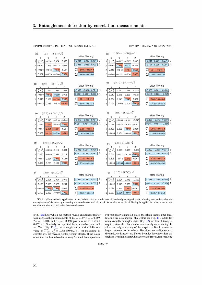
OPTIMIZED STATE-INDEPENDENT ENTANGLEMENT . . . PHYSICAL REVIEW A 88, 022327 (2013)
−0.057 −0.034 0.371
0.086 0.280 0.066
1.884+/−0.049>1
1.859+/−0.046>1
−0.012 −0.030 0.424
0.354 0.104 0.089
1.872+/−0.058>1
1.762+/−0.034>1
−0.006 0.091 0.430
0.187 0.088 0.353
1.773+/−0.039>1
1.773+/−0.039>1
−0.029 0.056 0.522
0.058 0.014 0.557
1.859+/−0.051>1
1.859+/−0.051>1
−0.079 0.001 0.460
−0.110 0.088 −0.454
1.763+/−0.036>1
1.763+/−0.036>1
−0.088 −0.175 0.339
0.015 0.151 −0.281
1.794+/−0.036>1
1.794+/−0.036>1
−0.029 −0.057 0.334
−0.290 −0.014 0.002
1.879+/−0.035>1
1.831+/−0.042>1
−0.038 −0.013 0.340
0.295 −0.025 −0.054
1.792+/−0.033>1
1.868+/−0.031>1
−0.084 0.091 0.371
−0.151 0.306 0.084
1.794+/−0.046>1
1.780+/−0.044>1
(b)
−0.190
0.064 0.027 0.022
−0.080 −0.229 0.053
0.042 0.039 0.959
−0.023 0.083 −0.204−0.915
Y
Z
X
X Y Z1
1 BA
(c)
0.945
0.010 0.031 −0.068
0.013 0.978 0.088 −0.072
0.034 0.048 0.067
0.047 −0.062 −0.9330.106
Y
Z
X
X Y Z1
1 BA
(d)
0.018 −0.010 −0.040
0.054 0.099 −0.082 0.941
−0.057 0.961 −0.054
0.082 −0.089−0.936
Y
Z
X
X Y Z1
1 BA
(e)
−0.967
−0.059 −0.131 −0.015
0.066 −0.916 −0.167 −0.197
0.105 0.089 0.031
−0.008 0.181 −0.927−0.093
Y
Z
X
X Y Z1
1 BA
(f)
0.977
−0.058 0.115 0.001
0.076 −0.899 0.081 0.219
−0.057 0.204 −0.069
0.082 0.266 0.9050.151
Y
Z
X
X Y Z1
1 BA
(g)
0.028 0.005 −0.058
0.044 −0.017 −0.110 −0.959
0.105 −0.014 −0.067
−0.008 −0.056−0.036
Y
Z
X
X Y Z1
1 BA
(h)
0.069
0.051 0.051 0.055
0.133 0.082 0.929 0.204
−0.034 0.007
0.109 0.053 0.962−0.159
Y
Z
X
X Y Z1
1 BA
(i)
0.021 0.015 −0.089
−0.092 0.110 0.098 0.952
0.022 0.157 −0.041
0.057 −0.055−0.007
Y
Z
X
X Y Z1
1 BA
(j)
−0.131
−0.087 −0.067 0.002
−0.062 0.951 −0.074 −0.164
0.045 −0.242 −0.933
−0.046 −0.113 0.053−0.954
Y
Z
X
X Y Z1
1 BA−0.114 0.024 0.052
−0.101 0.969 −0.023 0.058
−0.023 −0.013 −0.061
0.071 −0.073 0.984−0.008
Y
Z
X
X Y Z1
1 BA
(a)
−0.949
−0.034 −0.045 0.401
−0.031 −0.033 0.422
1.869+/−0.029>1
1.869+/−0.029>1
after filtering
B
A
after filtering
B
A
after filtering
B
A
after filtering
B
A
after filtering
B
A
after filtering
B
A
after filtering
B
A
after filtering
B
A
after filtering
B
A
after filtering
B
A
−0.091
−0.942
−0.194
0.964
−0.954
0.978
0.981
0.940
FIG. 11. (Color online) Application of the decision tree on a selection of maximally entangled states, allowing one to determine theentanglement of the state by measuring the correlations marked in red. As an alternative, local filtering is applied in order to extract thecorrelations with maximal value (blue correlations).
[Fig. 12(c)], for which our method reveals entanglement afterfour steps, as the measurements of Tzz = 0.007, Tyy = 0.069,Txx = −0.801, and Tyz = −0.968 give a value of 1.583 ±0.067 > 1. Similarly, as expected, for a separable state suchas |HH 〉 [Fig. 12(f)], our entanglement criterion delivers avalue of
∑3k,l=1 T 2
kl = 0.964 ± 0.062 < 1 for measuring allcorrelations, not revealing entanglement clearly. These states,of course, can be analyzed also using Schmidt decomposition.
For maximally entangled states, the Bloch vectors after localfiltering are also shown (blue color; see Fig. 11), while fornonmaximally entangled states (Fig. 12), no local filtering isrequired since the Bloch vectors are already nonvanishing. Inall cases, only one entry of the respective Bloch vectors islarge compared to the others. Therefore, no realignment ofthe analyzers is necessary. Due to Schmidt decomposition, thedecision tree should start with a correlation measurement along
022327-9
3. Entanglement detection by correlation measurements
64

WIESŁAW LASKOWSKI et al. PHYSICAL REVIEW A 88, 022327 (2013)
1.350+/−0.041>1−0.128
−0.090 0.087 0.367
−0.168 0.845 −0.068 −0.200
−0.290 −0.221 −0.911
0.067 −0.077 0.053−0.849
Y
Z
X
X Y Z1
1 BA
(a)
−0.618
−0.099 0.005 0.719
−0.083 0.649 0.031 −0.019
0.128 −0.130 0.160
0.704 −0.062 0.984−0.014
Y
Z
X
X Y Z1
1 BA
(b)
0.069
−0.075 −0.053 0.373
0.172 0.357
−0.393 −0.117 −0.968
−0.036 −0.071 0.842
Y
Z
X
X Y Z1
1 BA
(c)
−0.810
0.029 −0.004 0.455
0.053 0.806 −0.008 0.052
0.110 −0.114 0.134
0.441 −0.006 0.9940.044
Y
Z
X
X Y Z1
1 BA
(d)
0.118
0.349 −0.071 −0.108
0.104 0.069
−0.376 −0.976 −0.029
−0.104 0.016 0.108
Y
Z
X
X Y Z1
1 BA
(e)
−0.042
−0.027 −0.041 0.993
0.118 −0.022 0.028 0.128
−0.001 −0.033 0.039
0.982 −0.027 0.970−0.012
Y
Z
X
X Y Z1
1 BA
(f)
1.563+/−0.061>1
1.631+/−0.043>1
1.714+/−0.040>1
1.644+/−0.053>1
1.644+/−0.053>1
0.964+/−0.062<1
0.964+/−0.062<1
1.583+/−0.053>1
1.579+/−0.048>1
1.350+/−0.041>11.548+/−0.056>1
1
0.037−0.801
0.007
0.156-0.859
0.815
FIG. 12. (Color online) Application of the decision tree on a selection of nonmaximally entangled states, allowing one to determine theentanglement of the state by measuring the correlations marked in red. Due to the asymmetry of the states, local filtering is unnecessary, andthe information on the Bloch vectors can be used to detect entanglement with a maximal number of three correlation measurements (bluecorrelations). (f) For a product state, the full set of correlations does not reveal entanglement, as it should be.
a direction in which we see a big local expectation value. Insuch a case, it is sufficient to cyclically relabel the requiredmeasurements as defined for the original decision tree.Following this method, it is possible to detect entanglementwith a maximum number of three steps. The first correlation tobe measured is determined by the Bloch vectors after applyinglocal filtering.
2. Many qubits
For the demonstration of multiqubit entanglement detec-tion, we use a family of three-photon polarization entangledGdansk (G) states [23] and the four-qubit Dicke state. The Gstates are defined by
|G(α)〉 = cos(α)|W 〉 + sin(α)|W 〉, (23)
where |W 〉 = 1√3(|HHV 〉 + |HV H 〉 + |V HH 〉), and in or-
der to obtain |W 〉, one exchanges H and V . The four-qubitDicke state with two “excitations” reads
∣∣D(2)4
⟩ = 1√6
(|HHV V 〉 + |HV HV 〉 + |V HHV 〉+|HV V H 〉 + |V HV H 〉 + |V V HH 〉). (24)
Generalized three-qubit G state. In order to observe thesestates, a collinear type-II SPDC source together with a linear
setup to prepare the four-photon Dicke state D(2)4 is used
[24,25]. The three-photon state is obtained if thefirst photon is measured to be cos(α)|H 〉 + sin(α)|V 〉polarized.
The protocol for entanglement detection starts with ob-servers locally measuring the polarization of their respectivephotons, enabling them to individually determine the Blochvectors.
(i) For the G(π/4) state, we obtain Ti00 = (0.636,
−0.008,−0.015), T0j0 = (0.623,−0.092,0.010), and T00k =(0.636,0.070,0.022). The Bloch vectors suggest that thecorrelation Txxx is big. Therefore, the decision tree starts withthe measurement of Txxx = 0.904 ± 0.025 and continues withTxzz = −0.578 ± 0.025 (see Fig. 3). These two measurementsalready prove entanglement because T 2
xxx + T 2xzz = 1.152 ±
0.038 > 1.(ii) For the W state, G(π/2), the Bloch vectors are Ti00 =
(0.016,−0.070,0.318), T0j0 = (−0.010,−0.073,0.308), andT00k = (−0.011,−0.0547,0.319), which suggests that now thecorrelation Tzzz is big. Indeed, we observe Tzzz = −0.882 ±0.025. The decision tree is the same as above, but with localaxes renamed as follows: x → z → y → x. Therefore, thesecond measurement has to be Tzyy . With Tzyy = 0.571 ±0.025, we again prove entanglement as T 2
xxx + T 2zyy = 1.104 ±
0.037 > 1.
022327-10
3.3. Publications
65

OPTIMIZED STATE-INDEPENDENT ENTANGLEMENT . . . PHYSICAL REVIEW A 88, 022327 (2013)
Four-qubit Dicke state. Here, we have vanishingBloch vectors, Ti000 = (−0.020,−0.016,0.007), T0j00 =(−0.011,−0.029,0.014), T00k0 = (−0.018,−0.020,−0.004),and T000l = (−0.009,−0.022,0.008). We construct aset of mutually commuting operators, which form thefirst branch of the four-qubit decision tree starting withTzzzz{zzzz → zzxx → zxzx → zxxz → xzxz → xxzz →xzzx → xxxx → yyyy}. After measuring the correlations,Tzzzz = 0.848 ± 0.025, Tzzxx = −0.533 ± 0.025, Tzxzx =−0.552 ± 0.025, our algorithm succeeds since T 2
zzzz +T 2
zzxx + T 2zxzx = 1.3082 ± 0.041 > 1.
VI. CONCLUSIONS
The entanglement of arbitrary multiqubit states can beefficiently detected based on two methods described here.Both methods employ a criterion based on the sum of squaredcorrelations. Combining this with an adaptive determinationof the correlations to be measured allows one to succeedmuch faster than standard tomographic schemes. The firstone, particularly designed for two-qubit states, determinesthe Schmidt decomposition from local measurements only,
where at most three correlation measurements are sufficientfor entanglement detection. The second one employs adecision tree to speed up the analysis. Its design is based oncorrelation complementarity and prevents one from measuringless informative correlations. The performance of the schemeis numerically analyzed for arbitrary pure states and, in thetwo-qubit case, for mixed states. The schemes succeed, onaverage, at least one step earlier as compared with randomsampling on two-qubit states, with an exponentially increasingspeedup for a higher number of qubits. Our results encouragethe application of these schemes in state-of-the-art experimentswith quantum states of increasing complexity.
ACKNOWLEDGMENTS
We thank the EU-BMBF project QUASAR and the EUprojects QWAD and QOLAPS for supporting this work. T.P.acknowledges support by the National Research Foundation,the Ministry of Education of Singapore, start-up grant ofthe Nanyang Technological University, and NCN Grant No.2012/05/E/ST2/02352. C.S. thanks QCCC of the Elite Net-work of Bavaria for support.
[1] R. Horodecki, P. Horodecki, M. Horodecki, and K. Horodecki,Rev. Mod. Phys. 81, 865 (2009).
[2] J.-W. Pan, Z.-B. Chen, C.-Y. Lu, H. Weinfurter, A. Zeilinger,and M. Zukowski, Rev. Mod. Phys. 84, 777 (2012).
[3] M. A. Nielsen and I. Chuang, Quantum Computation andQuantum Information (Cambridge University Press, New York,2000).
[4] M. Horodecki, P. Horodecki, and R. Horodecki, Phys. Lett. A223, 1 (1996).
[5] M. Bourennane, M. Eibl, C. Kurtsiefer, S. Gaertner,H. Weinfurter, O. Guhne, P. Hyllus, D. Bruß, M. Lewenstein, andA. Sanpera, Phys. Rev. Lett. 92, 087902 (2004).
[6] B. M. Terhal, Phys. Lett. A 271, 319 (2000).[7] M. Lewenstein, B. Kraus, J. I. Cirac, and P. Horodecki, Phys.
Rev. A 62, 052310 (2000).[8] D. Bruß, J. I. Cirac, P. Horodecki, F. Hulpke, B. Kraus,
M. Lewenstein, and A. Sanpera, J. Mod. Opt. 49, 1399 (2002).[9] O. Guhne and P. Hyllus, Int. J. Theor. Phys. 42, 1001
(2003).[10] O. Guhne and G. Toth, Phys. Rep. 474, 1 (2009).[11] P. Badziag, C. Brukner, W. Laskowski, T. Paterek, and
M. Zukowski, Phys. Rev. Lett. 100, 140403 (2008).
[12] W. Laskowski, D. Richart, C. Schwemmer, T. Paterek, andH. Weinfurter, Phys. Rev. Lett. 108, 240501 (2012).
[13] P. Kurzynski, T. Paterek, R. Ramanathan, W. Laskowski, andD. Kaszlikowski, Phys. Rev. Lett. 106, 180402 (2011).
[14] E. Schmidt, Math. Ann. 63, 433 (1906).[15] A. Peres, Quantum Theory: Concepts and Methods (Kluwer
Academic, Dordrecht, 1995).[16] G. Toth and O. Guhne, Phys. Rev. A 72, 022340 (2005).[17] S. Wehner and A. Winter, J. Math. Phys. 49, 062105 (2008).[18] S. Wehner and A. Winter, New J. Phys. 12, 025009 (2010).[19] G. Vidal and R. F. Werner, Phys. Rev. A 65, 032314 (2002).[20] R. F. Werner, Phys. Rev. A 40, 4277 (1989).[21] P. G. Kwiat, E. Waks, A. G. White, I. Appelbaum, and P. H.
Eberhard, Phys. Rev. A 60, R773 (1999).[22] P. Trojek and H. Weinfurter, Appl. Phys. Lett. 92, 211103 (2008).[23] A. Sen(De), U. Sen, and M. Zukowski, Phys. Rev. A 68, 032309
(2003).[24] R. Krischek, C. Schwemmer, W. Wieczorek, H. Weinfurter, P.
Hyllus, L. Pezze, and A. Smerzi, Phys. Rev. Lett. 107, 080504(2011).
[25] N. Kiesel, C. Schmid, G. Toth, E. Solano, and H. Weinfurter,Phys. Rev. Lett. 98, 063604 (2007).
022327-11
3. Entanglement detection by correlation measurements
66

Genuine Multipartite Entanglement without Multipartite Correlations
Christian Schwemmer,1,2 Lukas Knips,1,2 Minh Cong Tran,3 Anna de Rosier,4 Wiesław Laskowski,4
Tomasz Paterek,3,5,6,* and Harald Weinfurter1,21Max-Planck-Institut für Quantenoptik, Hans-Kopfermann-Straße 1, 85748 Garching, Germany
2Department für Physik, Ludwig-Maximilians-Universität, 80797 München, Germany3School of Physical and Mathematical Sciences, Nanyang Technological University, Singapore, 637371 Singapore
4Institute of Theoretical Physics and Astrophysics, University of Gdańsk, PL-80-952 Gdańsk, Poland5Center for Quantum Technologies, National University of Singapore, Singapore, 117543 Singapore6MajuLab, CNRS-UNS-NUS-NTU International Joint Research Unit, Singapore, UMI 3654 Singapore
(Received 9 October 2014; published 6 May 2015)
Nonclassical correlations between measurement results make entanglement the essence of quantumphysics and the main resource for quantum information applications. Surprisingly, there are n-particlestates which do not exhibit n-partite correlations at all but still are genuinely n-partite entangled. Weintroduce a general construction principle for such states, implement them in a multiphoton experiment andanalyze their properties in detail. Remarkably, even without multipartite correlations, these states do violateBell inequalities showing that there is no classical, i.e., local realistic model describing their properties.
DOI: 10.1103/PhysRevLett.114.180501 PACS numbers: 03.67.Mn, 03.65.Ud, 42.50.Dv
Correlations between measurement results are the mostprominent feature of entanglement. They made Einstein,Podolski, and Rosen [1] question the completeness ofquantum mechanics and are nowadays the main ingredientfor the many applications of quantum information likeentanglement based quantum key distribution [2] orquantum teleportation [3].Correlations enable us, e.g., when observing two max-
imally entangled qubits, to use a measurement resultobserved on the first system to infer exactly the measure-ment result on the second system. In this scenario, the twoparticle correlations are formally given by the expectationvalue of the product of the measurement results obtained bythe two observers. Note, the single particle correlation, i.e.,the expectation value of the results for one or the otherparticle are zero in this case. Consequently, we cannotpredict anything about the individual results. When study-ing the entanglement between n particles, a natural exten-sion is to consider n-partite correlations, i.e., theexpectation value of the product of n measurement results.Such correlation functions are frequently used in classicalstatistics and signal analysis [4], moreover, in quantuminformation, almost all standard tools for analyzing multi-partite systems like multiparty entanglement witnesses[5,6] and Bell inequalities [7,8] are based on the n-partitecorrelation functions.Recently, Kaszlikowski et al. [9] pointed at a particular
quantum state with vanishing multiparty correlationswhich, however, is genuinely multipartite entangled.This discovery, of course, prompted vivid discussions ona viable definition of classical and quantum correlations[10,11]. Still, the question remains what makes up suchstates with no full n-partite correlations and how non-classical they can be, i.e., whether they are not onlyentangled but whether they also violate a Bell inequality.
Here, we generalize, highlight, and experimentally testsuch remarkable quantum states. We introduce a simpleprinciple how to construct states without n-partite cor-relations for odd n and show that there are infinitely manysuch states which are genuinely n-partite entangled. Weimplement three and five qubit no-correlation states in amultiphoton experiment and demonstrate that these statesdo not exhibit n-partite correlations. Yet, due to theexistence of correlations between a smaller number ofparticles, we observe genuine n-partite entanglement.Using our recently developed method to design n-partiteBell inequalities from lower order correlation functionsonly [12,13], we show that these states, despite not havingfull correlations, can violate Bell inequalities.Correlations.—The quantum mechanical correlation
function Tj1…jn is defined as the expectation value of theproduct of the results of n observers
Tj1…jn ¼ hr1…rni ¼ Trðρσj1 ⊗ … ⊗ σjnÞ; ð1Þ
where rk is the outcome of the local measurement of the kthobserver, parametrized by the Pauli operator σjk withjk ∈ fx; y; zg. Evidently, besides the n-partite correlations,for an n-partite state, one can also define l < n foldcorrelations Tμ1…μn ¼ Trðρσμ1 ⊗ … ⊗ σμnÞ with μi ∈f0; x; y; zg and jfμi ¼ 0gj ¼ n − l. Nonvanishing l-foldcorrelations indicate that we can infer (with higher proba-bility of success than pure guessing) an lth measurementresult from the product of the other ðl − 1Þ results [seeSupplemental Material [14]]. Only in the two particlescenario can we directly use the result from one measure-ment to infer the other result. For an n-qubit no-correlationstate, the vanishing n-partite correlations do not implyvanishing correlations between a smaller number of observ-ers, thus not necessarily destroying predictability. We will
PRL 114, 180501 (2015) P HY S I CA L R EV I EW LE T T ER Sweek ending8 MAY 2015
0031-9007=15=114(18)=180501(5) 180501-1 © 2015 American Physical Society
3.3. Publications
P3.3
67

see also in the experimentally implemented example that thevarious individual results still enable some possibility forinference, which is then largely due to bipartite correlations.Constructing no-correlation states.—For any state jψi
with an odd number n of qubits, we can construct an“antistate” jψi, i.e., the state whose n-partite correlationsare inverted with respect to the initial one. By evenlymixing these states
ρncψ ¼ 1
2jψihψ j þ 1
2jψihψ j; ð2Þ
we obtain a state ρncψ without n-partite correlations.The antistate jψi of a state jψi described in the computa-
tional basis by
jψi ¼X1
k1;…;kn¼0
αk1;…;kn jk1…kni; ð3Þ
with normalized coefficients αk1;…;kn ∈ C, is given by
jψi≡ X1k1;…;kn¼0
ð−1Þk1þ���þknα�1−k1;…;1−kn jk1…kni; ð4Þ
where the asterisk denotes complex conjugation. This statehas inverted correlations with respect to those in jψi forevery odd number of observers, whereas all the correlationfunction values for an even number of observers remainunchanged.jψi is mathematically obtained from jψi by applying
local universal-not gates [24]. These gates introduce aminus sign to all local Pauli operators. Therefore, for odd n,the correlations of jψi have opposite sign to those of jψi.Representing the universal-not gate by N ¼ σzσxK,where K is the complex conjugation operating in the com-putational basis, i.e., Kðαj0i þ βj1iÞ ¼ α�j0i þ β�j1i,indeed, we obtain NσxN† ¼ −σx, NσyN† ¼ −σy, andNσzN† ¼ −σz. Applying N to all the n subsystems, wefind the anticipated result N ⊗ � � � ⊗ Njψi ¼ jψi.Although N is antiunitary, jψi is always a proper
physical state and can be obtained by some global trans-formation of jψi. In general, N can be approximated [25],but if all the coefficients αk1…kn are real, complex con-jugation can be omitted and no-correlation states can begenerated by local operations.This construction principle can be generalized to mixed
states using ρ ¼ N⊗nρðN⊗nÞ†, which changes every purestate in the spectral form to the respective antistate. Evenlymixing ρ and ρ therefore produces a state with no l-partycorrelations for all odd l.One may then wonder whether the principle of Eq. (2)
can also be applied to construct a no-correlation state forevery state with an even number of qubits. The answer isnegative as shown by the following counterexample.Consider the Greenberger-Horne-Zeilinger state of an evennumber of qubits jψi ¼ ð1= ffiffiffi
2p Þðj0…0i þ j1…1iÞ. It has
nonvanishing Tz…z, 2n−1 multipartite correlations in the xyplane, and also, 2n−1 − 1 correlations between a smallernumber of subsystems, all equal to �1. However, for a statewith inverted correlations between all n parties (making noassumptions about the correlations between smaller numbersof observers), the fidelity relative to the GHZ state, given by12n
P3μ1;…;μn¼0 T
GHZμ1…μnT
antiμ1…μn , is negative because more than
half of the correlations are opposite. Hence, this state isunphysical and there is no such “antistate”. In fact, so far wewere unable to find an antistate to any genuinely multiqubitentangled state of even n.Entanglement without correlations: infinite family.—
Consider a three-qubit system in the pure state
jϕi¼ sinβcosαj001iþsinβsinαj010iþcosβj100i; ð5Þwhere α; β ∈ ð0; π=2Þ (which includes the state jWi withα ¼ π=3 and β ¼ cos−1ð1= ffiffiffi
3p Þ). Together with any local
unitary transformation thereof, this defines a three dimen-sional subspace of genuinely tripartite entangled stateswithin the eight dimensional space of three qubit states. Toshow that all the respective no-correlation states ρncϕ aregenuinely entangled, we use a criterion similar to the onein [6], i.e.,
maxTbi-prod
ðT;Tbi-prodÞ< ðT;TexpÞ⇒ρexp is not biseparable; ð6Þ
where maximization is over all biproduct pure states andðU;VÞ≡P
3μ;ν;η¼0UμνηVμνη denotes the inner product in
the vector space of correlation tensors. Condition[Eq. (6)] can be interpreted as an entanglementwitness W ¼ α1 − ρncϕ , where α ¼ L=8 and L ¼maxTbi-prodðT; TbiproductÞ is the left-hand side of Eq. (6). Inthe ideal case of preparing ρexp perfectly, Texp ¼ T, theright-hand side of our criterion equals four for all the statesof the family, and thus, the expectation value of the witnessis given by TrðWρncϕ Þ ¼ ðL − 4Þ=8.A simple argument for ρncϕ being genuinely tripartite
entangled can be obtained from the observation that jϕi andjϕi span a two-dimensional subspace of the three qubitHilbert space [9]. As none of the states jΦi ¼ ajϕi þ bjϕiis a biproduct (for the proof see Supplemental Material[14]), states in their convex hull do not intersect with thesubspace of biseparable states and thus all its states,including ρncϕ are genuinely tripartite entangled. To evaluatethe entanglement in the experiment, we calculated L for allstates of Eq. (5). We obtain Ljϕi < 4 in general, withLjWi ¼ 10=3. Similar techniques were used to analyzefive-qubit systems.Quantum correlations without classical correlations?—
The cumulants and correlations were initially proposedas a measure of genuinely multiparty nonclassicality inRef. [26]. Kaszlikowski et al. [9], however, showed thatsuch a quantification is not sufficient as the state ρncW has
PRL 114, 180501 (2015) P HY S I CA L R EV I EW LE T T ER Sweek ending8 MAY 2015
180501-2
3. Entanglement detection by correlation measurements
68

vanishing cumulants, yet contains genuinely multipartyentanglement. They suggested that the vanishing cumulantsor standard correlation functions [Eq. (1)] indicate the lackof genuine multiparty “classical” correlations. This initi-ated a vivid discussion on a proper definition and measureof genuine multipartite “classical” and quantum correla-tions. Bennett et al. proposed a set of axioms for measuresof genuine multipartite correlations [11]. They showed thatthe correlation function [Eq. (1)] does not fulfill all therequirements, but also still strive for computable measuresthat satisfy these axioms [15,27]. An information-theoreticdefinition of multipartite correlations was given by Giorgiet al. [15]. Their measure combines the entropy of all sizesof subsystems. Applying their definitions to ρncW , we obtaingenuine classical tripartite correlations of 0.813 bit andgenuine quantum tripartite correlations of 0.439 bit result-ing in total genuine tripartite correlations of 1.252 bit (seeSupplemental Material [14] for calculations for all ρncϕ ).While this approach does assign classical correlations in thecontext of Giorgi et al. [15] to ρncW , it does not fulfill allrequirements of [11] either.Experiment.—The three photon state jWi can be
observed either using a multiphoton interferometer setup[28] or by suitably projecting the fourth photon of a4-photon symmetric Dicke state [29]. The latter schemehas the advantage that it also offers the option to prepare thestates jWi and ρncW . The states jWi and jWi are particularrepresentatives of the symmetric Dicke states, which aredefined as
jDðeÞn i ¼
�ne
�−1=2X
i
PiðjH⊗ðn−eÞi ⊗ jV⊗eiÞ; ð7Þ
where jH=Vi denotes horizontal (vertical) polarization andPi all distinct permutations, and with the three photonstates jWi ¼ jDð1Þ
3 i and jWi ¼ jDð2Þ3 i. We observed four-
and six-photon Dicke states using a pulsed collinear type IIspontaneous parametric down conversion source togetherwith a linear optical setup (see Fig. 1) [30,31]. The jDðeÞ
n istates were observed upon detection of one photon in eachof the four or six spatial modes, respectively. We charac-terized the state jDð2Þ
4 i by means of quantum state tomog-raphy, i.e., a polarization analysis in each mode, collectingfor each setting 26 minutes of data at a rate of 70 events perminute. The fidelity of the experimental state jDð2Þ
4 iexp wasdirectly determined from the observed frequencies togetherwith Gaussian error propagation as 0.920� 0.005, whichdue to the high number of detected events [16] is com-patible with the value 0.917� 0.002 as obtained from amaximum likelihood (ML) reconstruction and nonpara-metric bootstrapping [14,20]. The high quality achievedhere allowed a precise study of the respective states. Thefidelities of the observed three qubit states with respectto their target states are 0.939� 0.011 for jWiexp,0.919� 0.010 for jWiexp, and 0.961� 0.003 for ρnc;expW .
Analogously, starting with a six-photon Dicke state jDð3Þ6 i
[32], we could also analyze the properties of the five photonstate ρnc
Dð2Þ5
. The five-qubit fidelity of ρnc;expDð2Þ
5
is determined
via a ML reconstruction from fivefold coincidences tobe 0.911� 0.004 (for the detailed characterization seeSupplemental Material [14]).For the experimental analysis of the states, we start by
determining Tzzz for the three states jWiexp, jWiexp, andρnc;expW . As the first two have complementary structure ofdetection probabilities (with Tzzz ¼ −0.914� 0.034 andTzzz ¼ 0.904� 0.034, respectively), weighted mixing ofthese states leads to ρnc;expW with Tzzz ¼ 0.022� 0.023, i.e.,a correlation value compatible with 0 (see SupplementalMaterial [14]). Figure 2 presents experimental data for allpossible tripartite correlations of the observed states.Assuming a normal distribution centered at zero with astandard deviation given by our experimental errors, theobserved correlations have a p value of 0.44 for theAnderson-Darling test, which shows that indeed one canadhere to the hypothesis of vanishing full correlations.Similarly, the five qubit state ρnc;exp
Dð2Þ5
exhibits strongly
suppressed, almost vanishing correlations. For details onthe five qubit state, please see Supplemental Material [14].We want to emphasize that the vanishing tripartite
correlations of ρnc;expW are no artifact of measuring in thePauli bases. In fact, all states obtained via local unitarytransformations do not exhibit any n-partite correlations.To illustrate this property, we considered correlationmeasurements in non-standard bases. As an example, wechose measurements in the zy plane σθ ¼ cos θσz þ sin θσywith θ ∈ ½0; 2π� (σϕ ¼ cosϕσy þ sinϕσz with ϕ ∈ ½0; 2π�)for the first (second) qubit resulting in the correlationsTθj2j3 ¼ Trðρσθ ⊗ σj2 ⊗ σj3Þ (Tj1ϕj3). Indeed, as shown in
SM
IF
BS1
QWP
HWP PBSPAj
APD
SPDC source
aPA
cPA
dPA
fPA
3BS
BS2
3SbPA
ePA
BS4 BS5
FIG. 1 (color online). Schematic of the linear optical setup usedto observe symmetric Dicke states from which states withvanishing 3- and 5-partite correlations can be obtained. Thephotons are created by means of a cavity enhanced pulsedcollinear type II spontaneous parametric down conversion sourcepumped at 390 nm [31]. Distributing the photons symmetricallyinto six modes by five beam splitters (BS) enables the observationof the state jDð3Þ
6 i. Removing beam splitters BS2 and BS4 reduces
the number of modes to four and thus the state jDð2Þ4 i is obtained.
State analysis is enabled by sets of half wave (HWP) and quarter-wave plates (QWP) together with polarizing beam splitters (PBS)in each mode. The photons are measured by fiber-coupled singlephoton counting modules connected to a coincidence logic [30].
PRL 114, 180501 (2015) P HY S I CA L R EV I EW LE T T ER Sweek ending8 MAY 2015
180501-3
3.3. Publications
69

Fig. 3, Tθj2j3 (Tj1ϕj3) vanishes independently of the choiceof θ (ϕ). In contrast, the bipartite correlations Tθz0 (Tyϕ0)between qubit 1 and 2 do not vanish at all and clearlydepend on θ (ϕ). By means of those even numbercorrelations, one is still able to infer the result of anotherparty from ones own result with probability 2=3 > 1=2. Forexample, the values of Tzz0 ¼ −1=3 (Tz0z ¼ −1=3) indi-cate that knowing, e.g., result “0” for the first qubit, we caninfer that the result will be “1” with p ¼ 2=3 on the second(third) qubit, etc.
Although the three qubits are not tripartite correlated, thebipartite correlations shown above give rise to genuinetripartite entanglement. This can be tested for the exper-imental states employing Eq. (6). We observe
ðT; Tnc;expW Þ ¼ 3.858� 0.079 > 3.333;
ðT; Tnc;exp
Dð2Þ5
Þ ¼ 13.663� 0.340 > 12.8;
both above the respective biseparable bound of 10=3 ¼3.333 (12.8) by more than 6.6 (2.4) standard deviations,proving that in spite of vanishing full correlations the statesare genuinely tripartite (five-partite) entangled [14].The observed five-photon state has one more remarkable
property [13]. For this state, every correlation between afixed number of observers, i.e., bipartite correlations,tripartite correlations, etc. admits description with anexplicit local hidden-variable model [8]. However, someof the models are different and thus cannot be combined ina single one. Using linear programming to find jointprobability distributions reproducing quantum predictions[12], we obtain an optimal Bell inequality using only two-and four-partite correlations [13]. From the observed data,we evaluate the Bell parameter to be B ¼ 6.358� 0.149which violates the local realistic bound of 6 by 2.4 standarddeviations [33]. This violation confirms the nonclassicality[14] of this no-correlation state and also offers its appli-cability for quantum communication complexity tasks.Contrary to previous schemes, here, the communicationproblem can be solved in every instance already by only asubset of the communicating parties [35].Conclusions.—We introduced a systematic way to
define and to experimentally observe mixed multipartitestates with no n-partite correlations for odd n, asmeasured by standard correlation functions. For the firsttime, we experimentally observed a state which allowed theviolation of a Bell inequality without full correlations,thereby proving both the nonclassicality of no-correlationstates as well as their applicability for quantum commu-nication protocols. The remarkable properties of thesestates prompt intriguing questions. For example, whatmight be the dimensionality of these states or theirrespective subspaces, or whether we can even extend thesubspace of states and antistates which give genuinelyentangled no-correlation states? Moreover, can no-correlation states be used for quantum protocols beyondcommunication complexity, and, of course, whether theseremarkable features can be cast into rigorous and easilycalculable measures of genuine correlations satisfyingnatural postulates [11]?
We thank the EU-BMBF Project No. QUASAR and theEU Project No. QWAD and No. QOLAPS for supportingthis work. T. P. acknowledges support by the NationalResearch Foundation, the Ministry of Education ofSingapore Grant No. RG98/13, Start-up Grant of the
XXX
XXY
XXZ
XYX
XYY
XYZ
ZZX
ZZY
ZZZ
0
0.4
0.8
-0.4
-0.8
0
0.4
0.8
-0.4
-0.8
0
0.04
-0.04
0.08
-0.08
noitalerroC
Wnc,exp
W exp
W exp
FIG. 2 (color online). Experimental tripartite correlations (red)for jWiexp, jWiexp, and (green) ρnc;expW in comparison to thetheoretically expected values (gray). Note that the correlations ofthe state ρnc;expW are magnified by a factor of 10. The plot presentsmeasured values of Tj1j2j3 for the observables listed below theplot. Obviously, the states jWiexp and jWiexp have oppositetripartite correlations canceling each other when they are mixed.
Phase Phase
Tr( )z
Tr( )zz
Tr( )z
Tr( )y
Tr( )yy
Tr( )y
0
0.2
0.6
0.4
-0.2
-0.6
-0.4
noitalerroC
FIG. 3 (color online). Vanishing tripartite correlations forarbitrary measurements and non-vanishing bipartite correlations.Observable σθ (σϕ) was measured on the first (second) qubit andσz (σy) measurements were performed on both other qubits (greencurves) or one of them (red and black curves). The solid linesshow the theoretically expected curves.
PRL 114, 180501 (2015) P HY S I CA L R EV I EW LE T T ER Sweek ending8 MAY 2015
180501-4
3. Entanglement detection by correlation measurements
70

Nanyang Technological University, and NCN GrantNo. 2012/05/E/ST2/02352. C. S. and L. K. thank theElite Network of Bavaria for support (Ph.D. ProgramsQCCC and ExQM).
*[email protected][1] A. Einstein, B. Podolsky, and N. Rosen, Phys. Rev. 47, 777
(1935).[2] A. K. Ekert, Phys. Rev. Lett. 67, 661 (1991).[3] C. H. Bennett, G. Brassard, C. Crépeau, R. Jozsa, A. Peres,
and W. K. Wootters, Phys. Rev. Lett. 70, 1895 (1993).[4] K. C. Chua, V. Chandran, U. R. Acharya, and C. M. Lim,
Medical Engineering and Physics 32, 679 (2010); J. M.Mendel, Proc. IEEE 79, 278 (1991).
[5] G. Tóth and O. Gühne, Phys. Rev. A 72, 022340 (2005); B.Lücke, J. Peise, G. Vitagliano, J. Arlt, L. Santos, G. Tóth,and C. Klempt, Phys. Rev. Lett. 112, 155304 (2014); J. I. deVicente and M. Huber, Phys. Rev. A 84, 062306 (2011); B.Jungnitsch, T. Moroder, and O. Gühne, Phys. Rev. Lett. 106,190502 (2011).
[6] P. Badziąg, Č. Brukner, W. Laskowski, T. Paterek, andM. Żukowski, Phys. Rev. Lett. 100, 140403 (2008); W.Laskowski, M. Markiewicz, T. Paterek, and M. Żukowski,Phys. Rev. A 84, 062305 (2011).
[7] J. F. Clauser, M. A. Horne, A. Shimony, and R. A. Holt,Phys. Rev. Lett. 23, 880 (1969); N. D. Mermin, Phys. Rev.D 22, 356 (1980); H. Weinfurter and M. Żukowski, Phys.Rev. A 64, 010102 (2001); R. F. Werner and M.M. Wolf,Phys. Rev. A 64, 032112 (2001); K. Nagata, W. Laskowski,and T. Paterek, Phys. Rev. A 74, 062109 (2006); W.Laskowski, T. Paterek, M. Żukowski, and Č. Brukner, Phys.Rev. Lett. 93, 200401 (2004); M. Ardehali, Phys. Rev. A 46,5375 (1992); A. V. Belinskiı and D. N. Klyshko, Phys. Usp.36, 653 (1993); D. Collins and N. Gisin, J. Phys. A 37, 1775(2004); T. Vértesi, Phys. Rev. A 78, 032112 (2008).
[8] M. Żukowski and Č. Brukner, Phys. Rev. Lett. 88, 210401(2002).
[9] D. Kaszlikowski, A. Sen De, U. Sen, V. Vedral, and A.Winter, Phys. Rev. Lett. 101, 070502 (2008).
[10] Z. Walczak, Phys. Lett. A 374, 3999 (2010); Z. Walczak,Phys. Rev. Lett. 104, 068901 (2010); D. Kaszlikowski, A.Sen De, U. Sen, V. Vedral, and A. Winter, Phys. Rev. Lett.104, 068902 (2010); K. Modi, A. Brodutch, H. Cable, T.Paterek, and V. Vedral, Rev. Mod. Phys. 84, 1655 (2012).
[11] C. H. Bennett, A. Grudka, M. Horodecki, P. Horodecki, andR. Horodecki, Phys. Rev. A 83, 012312 (2011).
[12] J. Gruca, W. Laskowski, M. Żukowski, N. Kiesel, W.Wieczorek, C. Schmid, and H. Weinfurter, Phys. Rev. A82, 012118 (2010).
[13] W. Laskowski, M. Markiewicz, T. Paterek, and M.Wieśniak, Phys. Rev. A 86, 032105 (2012).
[14] See Supplemental Material at http://link.aps.org/supplemental/10.1103/PhysRevLett.114.180501 for addi-tional information on physical meaning of the correlationfunctions, details about experimentally realized states,derivations of entanglement criteria used, and correlationcontent of the no-correlation states, which includes Refs.[9,13,15–23].
[15] G. L. Giorgi, B. Bellomo, F. Galve, and R. Zambrini, Phys.Rev. Lett. 107, 190501 (2011).
[16] C. Schwemmer, L. Knips, D. Richart, H. Weinfurter, T.Moroder, M. Kleinmann, and O. Gühne, Phys. Rev. Lett.114, 080403 (2015).
[17] G. Tóth, J. Opt. Soc. Am. B, 24, 275 (2007).[18] C. Schwemmer, G. Tóth, A. Niggebaum, T. Moroder, D.
Gross, O. Gühne, and H. Weinfurter, Phys. Rev. Lett. 113,040503 (2014).
[19] R. S. Bennink, Y. Liu, D. D. Earl, and W. P. Grice, Phys.Rev. A 74, 023802 (2006); P. Trojek, Ph.D. thesis, Ludwig-Maximilians-Universität München, 2007.
[20] B. Efron and R. J. Tibshirani, An Introduction to theBootstrap (Chapman & Hall, London, 1994).
[21] N. Kiesel, Ph.D. thesis, Ludwig-Maximilians-UniversitätMünchen, 2007.
[22] D. F. V. James, P. G. Kwiat, W. J. Munro, and A. G. White,Phys. Rev. A 64, 052312 (2001).
[23] J. Larsson, J. Phys. A 47, 424003 (2014).[24] V. Bužek, M. Hillery, and R. F. Werner, J. Mod. Opt. 47, 211
(2000).[25] F. de Martini, V. Bužek, F. Sciarrino, and C. Sias, Nature
(London) 419, 815 (2002); J. Bang, S.-W. Lee, H. Jeong,and J. Lee, Phys. Rev. A 86, 062317 (2012).
[26] D. L. Zhou, B. Zeng, Z. Xu, and L. You, Phys. Rev. A 74,052110 (2006).
[27] L. Zhao, X. Hu, R.-H. Yue, and H. Fan, Quantum Inf.Process. 12, 2371 (2013).
[28] M. Eibl, N. Kiesel, M. Bourennane, C. Kurtsiefer, and H.Weinfurter, Phys. Rev. Lett. 92, 077901 (2004).
[29] T. Yamamoto, K. Tamaki, M. Koashi, and N. Imoto, Phys.Rev. A 66, 064301 (2002); W. Wieczorek, N. Kiesel, C.Schmid, and H. Weinfurter, Phys. Rev. A 79, 022311(2009).
[30] N. Kiesel, C. Schmid, G. Tóth, E. Solano, and H. Weinfurter,Phys. Rev. Lett. 98, 063604 (2007); G. Tóth, W. Wieczorek,D. Gross, R. Krischek, C. Schwemmer, and H. Weinfurter,Phys. Rev. Lett. 105, 250403 (2010); R. Krischek, C.Schwemmer, W. Wieczorek, H. Weinfurter, P. Hyllus, L.Pezzé, and A. Smerzi, Phys. Rev. Lett. 107, 080504 (2011).
[31] R. Krischek, W. Wieczorek, A. Ozawa, N. Kiesel, P.Michelberger, T. Udem, and H. Weinfurter, Nat. Photonics4, 170 (2010).
[32] W. Wieczorek, R. Krischek, N. Kiesel, P. Michelberger, G.Tóth, and H. Weinfurter, Phys. Rev. Lett. 103, 020504(2009).
[33] Examples of Bell inequalities involving lower order corre-lations can be found in [34], however, none of them isviolated by our state ρnc
Dð2Þ5
.[34] M. Wieśniak, M. Nawareg, and M. Żukowski, Phys. Rev. A
86, 042339 (2012); J. Tura, R. Augusiak, A. B. Sainz, T.Vértesi, M. Lewenstein, and A. Acín, Science 344, 1256(2014); J. Tura, A. B. Sainz, T. Vértesi, A. Acín, M.Lewenstein, and R. Augusiak, J. Phys. A 47, 424024(2014).
[35] Č. Brukner, M. Żukowski, J.-W. Pan, and A. Zeilinger,Phys. Rev. Lett. 92, 127901 (2004); P. Trojek, C. Schmid,M. Bourennane, Č. Brukner, M. Żukowski, and H.Weinfurter, Phys. Rev. A 72, 050305 (2005); M. Wieśniak,arXiv:1212.2388.
PRL 114, 180501 (2015) P HY S I CA L R EV I EW LE T T ER Sweek ending8 MAY 2015
180501-5
3.3. Publications
71
Genuine n-partite entanglement without n-partite correlationsSUPPLEMENTAL MATERIAL
Christian Schwemmer,1, 2 Lukas Knips,1, 2 Minh Cong Tran,3 Anna de Rosier,4
Wies law Laskowski,4 Tomasz Paterek,3, 5, 6, ∗ and Harald Weinfurter1, 2
1Max-Planck-Institut fur Quantenoptik, Hans-Kopfermann-Straße 1, 85748 Garching, Germany2Department fur Physik, Ludwig-Maximilians-Universitat, 80797 Munchen, Germany
3School of Physical and Mathematical Sciences, Nanyang Technological University, 637371 Singapore4Institute of Theoretical Physics and Astrophysics,University of Gdansk, PL-80-952 Gdansk, Poland
5Centre for Quantum Technologies, National University of Singapore, 117543 Singapore6MajuLab, CNRS-UNS-NUS-NTU International Joint Research Unit, UMI 3654, Singapore
I. PHYSICAL MEANING OF CORRELATION FUNCTIONS
Correlations for two particles are often seen as a measure of predictability of local results when knowing the otherresult. Yet, this simple statement has to be used carefully. A non-vanishing n-partite correlation function indicatesthat we can make an educated guess of the nth result from the product of the other n − 1 results. The conversestatement does not hold and we provide an example of a state with vanishing correlation functions where the inferenceis still possible.
Let us denote by rj = ±1 the result of the jth observer. We assume that n−1 parties cannot infer from the productof their outcomes, r1 . . . rn−1, the result of the last observer, rn, i.e., the following conditional probabilities hold:
P (rn|r1 . . . rn−1) =1
2. (1)
We show that this implies that the corresponding correlation function, Tj1...jn , vanishes. The correlation function isdefined as expectation value of the product of all local outcomes
Tj1...jn = 〈r1 . . . rn〉 = P (r1 . . . rn = 1)− P (r1 . . . rn = −1). (2)
Using Bayes’ rule
P (r1 . . . rn = ±1) =∑r=±1
P (rn = ±r|r1 . . . rn−1 = r)P (r1 . . . rn−1 = r). (3)
According to assumption (1) we have P (rn = ±r|r1 . . . rn−1 = r) = 12 , giving P (r1 . . . rn = ±1) = 1
2 and Tj1...jn = 0.As an example of a state with vanishing correlation functions yet allowing to make an educated guess of the result,
let us consider the two-qubit mixed state
1
2|00〉 〈00|+ 1
4|01〉 〈01|+ 1
4|10〉 〈10| , (4)
where |0〉 and |1〉 are the eigenstates of the Pauli operator σz with eigenvalues +1 and −1, respectively. All correlationfunctions Tkl, with k, l = x, y, z, of this state vanish. Yet, whenever Alice (Bob) observes outcome −1 in the σzmeasurement, she (he) is sure the distant outcome is +1, i.e., P (r2 = +1|r1 = −1) = 1. Similar examples exist formultiple qubits, but we note that the states ρncφ of the main text are an equal mixture of a state and its anti-state.In this case, the vanishing n-party correlations lead to the impossibility of inferring the n-th result.
II. CRITERION FOR GENUINE MULTIPARTITE ENTANGLEMENT
To evaluate entanglement we use the following criterion (see main text) where, T exp = T , i.e., assuming the idealexperiment producing the required state described by the correlation tensor T :
maxT bi−prod
(T, T bi−prod) < (T, T ). (5)
3. Entanglement detection by correlation measurements
72

2
The maximization is performed over all bi-product states keeping in mind also all possible bipartitions. The innerproduct between two correlation tensors of three qubit states is defined as
(V,W ) ≡3∑
µ,ν,η=0
VµνηWµνη. (6)
A. Tripartite entanglement
To keep the statement as general as possible, we prove that all states ρncφ = 12 |φ〉 〈φ|+
12
∣∣φ⟩ ⟨φ∣∣ with
|φ〉 = sinβ cosα |001〉+ sinβ sinα |010〉+ cosβ |100〉 , (7)∣∣φ⟩ = sinβ cosα |110〉+ sinβ sinα |101〉+ cosβ |011〉 , (8)
are genuinely tripartite entangled as soon as |φ〉 is genuinely tripartite entangled.First, note that |φ〉 is a bi-product state if at least one amplitude vanishes, i.e., if either
1. β = 0 (full product state),
2. β = π2 and α = 0 (full product state),
3. β = π2 and α = π
2 (full product state),
4. β = π2 and α ∈ (0, π2 ) (bi-product A|BC),
5. α = 0 and β ∈ (0, π2 ) (bi-product B|AC),
6. α = π2 and β ∈ (0, π2 ) (bi-product C|AB).
The correlation tensor of the state ρncφ contains only bipartite correlations:
Txx0 = Tyy0 = sin(2β) sin(α),
Tx0x = Ty0y = sin(2β) cos(α),
T0xx = T0yy = sin2(β) sin(2α),
Tzz0 = cos(2α) sin2(β)− cos2(β),
Tz0z = − cos(2α) sin2(β)− cos2(β),
T0zz = cos(2β), (9)
and T000 = 1. Using these expressions, the right-hand side of the entanglement criterion is
R = (T, T ) = 4. (10)
To find the maximum of the left-hand side, we shall follow a few estimations. Consider first the bi-product state ina fixed bipartition, say AB|C, i.e., of the form |χ〉AB ⊗ |c〉, where |χ〉AB = cos(θ) |00〉 + sin(θ) |11〉, when written in
the Schmidt basis. Let us denote the correlation tensor of |χ〉AB with P and its local Bloch vectors by ~a and ~b. Wetherefore have:
L = 1 + Txx0(Pxx + Pyy) + Tzz0Pzz + Tx0x(axcx + aycy) + Tz0zazcz + T0xx(bxcx + bycy) + T0zzbzcz. (11)
By optimizing over the states of |c〉 we get the following upper bounds:
Tx0x(axcx + aycy) + Tz0zazcz ≤√T 2x0x(a2x + a2y) + T 2
z0za2z, (12)
and
T0xx(bxcx + bycy) + T0zzbzcz ≤√T 20xx(b2x + b2y) + T 2
0zzb2z. (13)
The Schmidt decomposition implies for local Bloch vectors:
a2x + a2y + a2z = b2x + b2y + b2z = cos2(2θ), (14)
3.3. Publications
73

3
and therefore
~a = cos(2θ)~n, ~b = cos(2θ)~m, (15)
where ~n and ~m are normalized vectors with directions along the local Bloch vectors. This gives the bound√T 2x0x(a2x + a2y) + T 2
z0za2z +
√T 20xx(b2x + b2y) + T 2
0zzb2z
= cos(2θ)(√
T 2x0x(n2x + n2y) + T 2
z0zn2z +
√T 20xx(m2
x +m2y) + T 2
0zzm2z
)≤ cos(2θ) (max(|Tx0x|, |Tz0z|) + max(|T0xx|, |T0zz|)) , (16)
where the maxima follow from convexity of squared components of a normalized vector.Now let us focus on the terms depending on the correlations of |χ〉AB . In order to maximize (11), the Schmidt
basis of |χ〉AB has to be either x, y, or z as otherwise off-diagonal elements of P emerge leading to smaller valuesentering (11). For the diagonal correlation tensor we have |Pxx| = sin(2θ), |Pyy| = sin(2θ), and Pzz = 1, and withindices permuted. Therefore, there are three cases to be considered in order to optimize Txx0(Pxx + Pyy) + Tzz0Pzz:
(i) |Pxx| = 1 and |Pyy| = |Pzz| = sin(2θ) with their signs matching those of Txx0 and Tzz0 respectively,
(ii) |Pzz| = 1 and Pxx = Pyy = sin(2θ),
(iii) |Pzz| = 1 and Pxx = −Pyy = sin(2θ).
Each of these cases leads to an upper bound on L. For example, for the first case we find
L(i) = 1 + |Txx0|+ sin(2θ)(|Txx0|+ |Tzz0|) + cos(2θ)(max(|Tx0x|, |Tz0z|) + max(|T0xx|, |T0zz|))
≤ 1 + |Txx0|+√
(|Txx0|+ |Tzz0|)2 + (max(|Tx0x|, |Tz0z|) + max(|T0xx|, |T0zz|))2, (17)
where in the last step we optimized over θ. The same procedure applied to the other two cases gives:
L(ii) ≤ 1 + |Tzz0|+√
4T 2xx0 + (max(|Tx0x|, |Tz0z|) + max(|T0xx|, |T0zz|))2, (18)
L(iii) ≤ 1 + |Tzz0|+ max(|Tx0x|, |Tz0z|) + max(|T0xx|, |T0zz|). (19)
If instead of the bipartition AB|C another one was chosen, the bounds obtained are given by those above with theindices correspondingly permuted. Since there are three possible bipartitions, altogether we have nine bounds out ofwhich we should finally choose the maximum as the actual upper bound on the left-hand side.
Numerical derivation of bounds
A first approach is to numerically evaluate Eqs. (17)-(19). Fig. 1 shows that only for states |φ〉 that are bi-productthe left-hand side reaches L = 4.
For theW state we thus obtain maxL = 10/3 which is achieved by the bi-product state (cos θ |++〉−sin θ |−−〉)⊗|+〉,where |±〉 = 1√
2(|0〉 ± |1〉) and tan(2θ) = 3/4 in order to optimize case (i) which is the best for the W state. This
bound is used in the main text.
Analytic argument
The last step of the proof, showing that only bi-separable states can achieve the bound of 4 in our criterion, involvednumerical optimization (Fig. 1). One may complain that due to finite numerical precision there might be genuinelytripartite entangled states for values of α or β close to 0 and π/2 that already achieve the bound of 4. Here, we givea simple analytical argument showing that ρncφ is genuinely tripartite entangled if and only if |φ〉 is so.
We first follow the idea of Ref. [9] and note that a mixed state ρncφ can only be bi-separable if there are bi-product
pure states in its support. The support of ρncφ is spanned by |φ〉 and |φ〉, i.e., ρncφ does not have any overlap with the
orthogonal subspace 11 − |φ〉 〈φ| − |φ〉〈φ|. Accordingly any decomposition of ρncφ into pure states can only use purestates of the form
|Φ〉 = a |φ〉+ b|φ〉. (20)
3. Entanglement detection by correlation measurements
74

4
3.4
3.5
3.6
3.7
3.8
3.9
1/8 π
1/4 π
3/8 π
1/2 π
α
00
1/8 π 1/4 π 3/8 π 1/2 π
β
FIG. 1. Contour plot showing the maximal value of the left-hand side of our entanglement criterion for the states ρncφ definedabove (7). Whenever the value is below 4, i.e., the right-hand side value as given in (10), the criterion detects genuine tripartiteentanglement. This shows that all the states ρncφ are genuinely tripartite entangled except for those arising from bi-productstates |φ〉, i.e., for α, β = 0 or π/2. Numerical optimizations over all bi-separable states yield the same plot.
We now give a simple argument that |Φ〉 is bi-product, and hence ρncφ is bi-separable, if and only if |φ〉 is bi-product.
In all other infinitely many cases, the no-correlation state is genuinely tripartite entangled. Assume that |Φ〉 is bi-product in the partition AB|C. Accordingly, all its correlation tensor components factor across this partition. Inparticular,
T0xx = W0xVx, T0yy = W0yVy, T0xy = W0xVy, T0yx = W0yVx (21)
where W is the correlation tensor of the state of AB and V is the correlation tensor corresponding to the state of C.One directly verifies that for such a bi-product state we have
T0xxT0yy = T0xyT0yx. (22)
Evaluating condition (22) for the states |Φ〉 gives the following condition on the amplitudes of |φ〉:
sin2(2α) sin4(β) = 0, (23)
and indicates that at least one amplitude must be zero. Similar reasoning applies to other partitions and we concludethat |Φ〉 is bi-product if and only if |φ〉 is bi-product.
Alternative entanglement criterion
Alternativly we can apply a witness of genuine tripartite entanglement based on angular momentum operators [17],
W3 = J2x + J2
y , (24)
where e.g. Jx = 12 (σx ⊗ 11 ⊗ 11 + 11 ⊗ σx ⊗ 11 + 11 ⊗ 11 ⊗ σx). Maximization of this quantity over bi-separable states
gives [17]:
maxρbi−sep
〈W3〉 = 2 +√
5/2 ≈ 3.12. (25)
This criterion detects entanglement of the states |φ〉 and∣∣φ⟩, and, consequently, since it uses two-party correlations
only, also of the state ρncφ . However, entanglement is detected only for a range of roughly α ∈ [0.590, 1.31] and
β ∈ [0.333, 1.24].
3.3. Publications
75

5
B. Five-partite entanglement
In order to obtain the five-partite bound given in the main text, i.e., maxT bi−prod(T, T bi−prod) = 12.8, we havenumerically optimized over all bi-product states keeping T as the correlation tensor of an equal mixture of Dicke
states |D(2)5 〉 and |D(3)
5 〉, where
|D(e)n 〉 =
1√(ne
) ∑i
|Pi(1, . . . , 1, 0 . . . , 0)〉, (26)
with Pi denoting all distinct permutations of e ones and n− e zeros.Below, we generalize the analytical argument given above to prove genuine multipartite entanglement of arbitrary
mixtures of Dicke and anti-Dicke states. The anti-Dicke state has exchanged roles of zeros and ones as comparedwith the Dicke state, i.e., it has n − e ones (excitations). One easily verifies that the Dicke state of n qubits with eexcitations has the following bipartite correlations:
T0...0xx = T0...0yy =2(n−2e−1)(
ne
) =2e(n− e)n(n− 1)
,
T0...0xy = T0...0yx = 0. (27)
The correlations of an anti-Dicke state, with n− e excitations, are the same due to the symmetry e↔ n− e of thesecorrelations. Assume that n is odd so that (i) the Dicke and anti-Dicke states are orthogonal and (ii) the parity of thenumber of excitations, i.e., whether there is an even or odd number of them, is opposite in the Dicke and anti-Dicke
states. For arbitrary superposition α|D(e)n 〉+ β|D(n−e)
n 〉 the correlations read:
T0...0jk = |α|2TD0...0jk+ |β|2TD0...0jk+α∗β〈D(e)n |11⊗ . . . 11⊗σj⊗σk|D(n−e)
n 〉+αβ∗〈D(n−e)n |11⊗ . . . 11⊗σj⊗σk|D(e)
n 〉. (28)
Since applying σj ⊗σk with j, k = x, y to the Dicke states does not change the parity of their excitations, the last two
terms vanish, and for the first two terms we have TD0...0jk = TD0...0jk. Therefore, an arbitrary superposition of Dicke
and anti-Dicke states has the same correlations as in (27) and therefore none of such superposed states is bi-product.Since the Dicke states are invariant under exchange of parties (and so are their superpositions), the same holds forother partitions. Finally, the lack of bi-product states in a subspace spanned by Dicke and anti-Dicke states impliesthat their mixtures are also genuinely multipartite entangled.
III. GENUINE TRIPARTITE CORRELATIONS
While the conventional full correlation function vanishes for ρncφ , this is not necessarily so for other types ofcorrelation functions introduced recently. For a comparison we analyze the correlation content of the states of ourfamily also according to the three measures given in Ref. [15], namely: (a) genuine tripartite correlations T (3)(ρncφ ),
(b) genuine tripartite classical correlations J (3)(ρncφ ), and (c) genuine tripartite quantum correlations D(3)(ρncφ ). Theresults are presented and discussed in Fig. 2.
3. Entanglement detection by correlation measurements
76

6
1/8 π
1/4 π
3/8 π
1/2 π
α
00
1/8 π 1/4 π 3/8 π 1/2 π
β
α
1/8 π
1/4 π
3/8 π
1/2 π
00 1/8 π 1/4 π 3/8 π 1/2 π
β
1/8 π
1/4 π
3/8 π
1/2 π
α
00
1/8 π 1/4 π 3/8 π 1/2 π
β
0
0.2
0.4
0.6
0.8
1
1.2
a) b)
c)
FIG. 2. Correlation content [15] of the states ρncφ = 12|φ〉 〈φ|+ 1
2
∣∣φ⟩ ⟨φ∣∣ with the pure states given in Eq. (7). (a) Total genuinetripartite correlations. The genuine tripartite correlations vanish only for mixtures of bi-product states. The highest value(1.2516) is obtained for the state (|W 〉〈W | + |W 〉〈W |)/2. (b) Genuine tripartite classical correlations. The genuine classicalcorrelations also vanish only for mixtures of bi-product states. The highest value (1.0) is observed for fully separable states.The local maximum (0.8127) is achieved by the state (|W 〉〈W | + |W 〉〈W |)/2. (c) Genuine tripartite quantum correlations.The genuine quantum correlations vanish for mixtures of bi-product states and for fully separable states. The highest values(0.6631) correspond to the mixture of the state
√1/6|001〉 +
√1/6|010〉 +
√2/3|100〉 with its antistate (and permutations).
The state (|W 〉〈W |+ |W 〉〈W |)/2 achieves the local maximum (0.4389).
IV. EXPERIMENTAL THREE AND FIVE QUBIT STATES
The experimentally prepared states |W 〉exp,∣∣W⟩exp, ρnc,expW , and ρnc,exp
D(2)5
were characterized by means of quantum
state tomography. Their corresponding density matrices can be seen in Fig. 3 and Fig. 4. The fidelities of theobserved three qubit states with respect to their target states are 0.939±0.011 for |W 〉exp, 0.919±0.010 for
∣∣W⟩exp, and0.961±0.003 for ρnc,expW . Note that the value of the fidelity for the state ρnc,expW was obtained from a maximum likelihood(ML) reconstruction together with non-parametric bootstrapping. This value thus might be slightly incorrect due tothe bias of the maximum likelihood data evaluation [16].
Fig. 4 shows the real part of the tomographically determined no-correlation state from which all further five qubitresults are deduced. The five-qubit fidelity of ρnc,exp
D(2)5
is determined via a ML reconstruction from five-fold coincidences
to be 0.911± 0.004.
To obtain a correlation function value, e.g., Tzzz = Tr(ρ σz ⊗ σz ⊗ σz), we analyze the three photons in therespective set of bases (here all z). Fig. 5 shows the relative frequencies for observing all the possible results for sucha polarization analysis. Clearly one recognizes the complementary structure of the the detection frequencies for thestates |W 〉exp and
∣∣W⟩exp which results in approximately the same magnitude of the correlations, yet with differentsign. Mixing the two states, one thus obtains a vanishingly small correlation. Fig. [2] of the main text then shows thefull set of correlations.
For the analysis of the five qubit no correlation state, we see from an eigen decomposition that this state indeed
comprises of a mixture of two states (|Θ(2)〉exp and |Θ(3)〉exp), which are in very good agreement with |D(2)5 〉 and
|D(3)5 〉. Fig. 6 (a) and (b) show all symmetrized correlations for the five-qubit states |Θ(2)〉 and |Θ(3)〉 and ρnc,exp
D(2)5
with
good agreement with the ideal states. Also the respective fidelity of the eigenvectors of the experimentally determinedstate are quite high (F|D(2)
5 〉(|Θ(2)〉) = 0.978±0.012 and F|D(3)
5 〉(|Θ(3)〉exp) = 0.979±0.012). Equally mixing the states
3.3. Publications
77

7
|Θ(2)〉exp and |Θ(3)〉exp indeed would result in a state with vanishingly small correlations as seen in Fig. 6 (c). However,due to asymmetry in the coupling of signal and idler states from the down conversion source [19] the correlations are
still present, albeit smaller by a factor of 10 compared with |D(2)5 〉 and |D(3)
5 〉. In the main text we show that the verysame state is genuinely five-party entangled.
FIG. 3. Experimental three qubit states as obtained from the state |D(2)4 〉exp. (a) The state |W 〉exp is obtained by projection
of the fourth qubit of |D(2)4 〉exp on V . (b) The state
∣∣W⟩exp is prepared by projecting the fourth qubit of |D(2)4 〉exp on H.
(c) When the fourth qubit of |D(2)4 〉exp is traced out, a mixture of |W 〉exp and
∣∣W⟩exp is obtained, i.e., the state ρnc,expW .
The corresponding fidelities with respect to their target states are 0.939 ± 0.011 for |W 〉exp, 0.919 ± 0.010 for∣∣W⟩exp, and
0.961± 0.003 for ρnc,expW .
FIG. 4. Experimental state ρnc,expD
(2)5
determined from five-fold coincidences together with permutational invariant tomogra-
phy [18]. The fidelity with respect to the target state is 0.911± 0.004.
3. Entanglement detection by correlation measurements
78

8
0
0.10
0.20
0.30
HH
HH
HV
HV
HH
VV
VH
HV
HV
VV
HV
VV
HH
HH
HV
HV
HH
VV
VH
HV
HV
VV
HV
VV
HH
HH
HV
HV
HH
VV
VH
HV
HV
VV
HV
VV
0.40 T =0.022zzzT =0.904zzzT =-0.914zzz
rWnc,exp
rel. f
req
ue
ncie
s
÷Wñexp÷Wñexp÷
FIG. 5. (color online). Detection frequencies when observing the states |W 〉exp (red) and∣∣W⟩exp (blue) and ρnc,expW (red and
blue) in the σ⊗3z basis. From these data Tzzz values can be calculated showing how the correlations of |W 〉exp and
∣∣W⟩expaverage to approximately 0. For comparison, the theoretically expected values are shown in gray. The correlation value Tzzz ofthe state ρnc,expW was determined as the weighted sum of the correlation values Tzzz of the states |W 〉exp and
∣∣W⟩exp. The state
|W 〉exp was observed with a slightly lower probability (0.485) than the state∣∣W⟩exp (0.515) leading to a value of Tzzz = 0.022
for the state ρnc,expW . In contrast, in Fig. 2 of the main text the states |W 〉exp and∣∣W⟩exp were obtained from the state |D(2)
4 〉expby projection of the fourth qubit onto horizontal/vertical polarization, i.e., from measuring σz on the fourth qubit. There,
ρnc,expW was obtained by tracing out the fourth qubit and hence measurements of σx, σy, σz on the fourth qubit of |D(2)4 〉exp
contribute, leading to approximately three times better statistics for the state ρnc,expW .
3.3. Publications
79

9
XX
XX
XX
XX
XY
XX
XY
YX
XY
YY
XY
YY
YY
YY
YY
XZZZZ
YZZZZ
ZZZZZ
XX
XX
ZX
XX
YZ
XX
YY
ZX
YY
YZ
YY
YY
ZX
XX
ZZ
XX
YZZ
XY
YZZ
YY
YZZ
XX
ZZZ
XY
ZZZ
YY
ZZZ
0
0.4
0.8
-0.4
-0.8
0
0.4
0.8
-0.4
-0.8
0
0.04
-0.04
0.08
-0.08
Co
rre
latio
n
0
0.04
-0.04
0.08
-0.08
rnc,exp
D5
(2)
á expq (2)÷0.5÷ ñq(2) á expq(3)
÷0.5÷ ñq(3)+
÷q(2) expñ(a)
(b)
(c)
(d)
÷q(3) expñ
FIG. 6. Experimental five-partite symmetric correlations for the two most prominent states (a) |Θ(2)〉exp and (b) |Θ(3)〉expin the eigen decomposition of the experimental density matrix ρnc,exp
D(2)5
shown in Fig. 4. The correlations of these states are
compared with the ones of the states (a) |D(2)5 〉 and (b) |D(3)
5 〉, respectively, shown in gray. The agreement between the actual
and expected correlations is evident and also the fidelities of |Θ(2)〉exp and |Θ(3)〉exp with the respective target states are
high: F|D(2)5 〉
(|Θ(2)〉exp) = 0.978 ± 0.012 and F|D(3)5 〉
(|Θ(3)〉exp) = 0.979 ± 0.012. (c) When both states are evenly mixed, the
resultant state has practically vanishing correlations. (d) Since the collection efficiencies for signal and idler photons generated
via spontaneous parametric down-conversion differ slightly [19], the states |Θ(2)〉exp and |Θ(3)〉exp are observed with relativeweights of 0.54 and 0.46 leading to largely suppressed but not entirely vanishing full correlations. Hence, the experimentallyprepared state ρnc,exp
D(2)5
is a very good approximation to a no-correlation state. Please note that the correlations shown in (c)
and (d) are magnified by a factor of 10 compared with the scale of (a) and (b). The errors given in subfigures (a)-(c) wereobtained by non-parametric bootstrapping [20] whereas for (d) Gaussian error propagation was used.
3. Entanglement detection by correlation measurements
80

10
V. STATISTICAL ANALYSIS
A. Error analysis
In order to carry out n-qubit quantum state tomography, we measured in the eigenbases of all 3n combinationsof local Pauli settings si with s1 = x...xx, s2 = x...xy, ..., s3n = z...zz. In each setting si we performed projectionmeasurements on all the 2n eigenvectors of the corresponding operators. The single measurement results are enu-merated by rj representing the binary numbers from 0 to 2n − 1 in increasing order, i.e., r1 = 0...00, r2 = 0...01, ...,r2n = 1...11. The observed counts for the outcome rj when measuring si are labeled as csirj and the total number of
counts Nsi for setting si is given by Nsi =2n∑j=1
csirj . From these data the density matrix can be obtained as
ρ =
3n∑i=1
2n∑j=1
csirjNsi
Msirj (29)
where the elements of the generating set of operators Msirj are defined as Msi
rj = 12n
n⊗k=1
(113 + (−1)rj(k)σsi(k)
)[21, 22],
where 11 denotes the 2 × 2 identity matrix and rj(k) is the k-th entry in the string rj . Then, the fidelity F|ψ〉 withrespect to a pure target state |ψ〉 can be calculated as
F|ψ〉 = 〈ψ| ρ |ψ〉 =3n∑i=1
2n∑j=1
csirjNsi〈ψ|Msi
rj |ψ〉 . (30)
For Poissonian measurement statistics, i.e., ∆csirj =√csirj , the error to the fidelity ∆F|ψ〉 =
√∆2F|ψ〉 can be deduced
via Gaussian error propagation as ∆2F|ψ〉 =3n∑i=1
2n∑j=1
( 1Nsi− 1
N2si
)2 〈ψ|Msirj |ψ〉
2csirj which is approximately
∆2F|ψ〉 =3n∑i=1
∆2F si|ψ〉 =3n∑i=1
2n∑j=1
csirjN2si
〈ψ|Msirj |ψ〉
2(31)
for large number of counts per setting as in our experiment. As an example, in table I we give the correspondingvalues for csirj and |〈ψ|Msi
rj |ψ〉| for the 23 = 8 possible results of the zzz measurement of the three qubit |W 〉 state to
get an impression of the size of the 33 = 27 terms in Eq. (31).
TABLE I. The values of csirj and |〈ψ|Msirj |ψ〉| for the measurement of the setting zzz of the experimentally observed state |W 〉exp.
The first row shows all possible results rj associated with the eigenvectors on which projection measurements are performed,labeled in binary representation. Please note that the observed counts csirj are not integers since the slightly differing relativedetection efficiencies of the single photon counters were included. From these data we obtain for si = zzz a contribution forEq. (31) of ∆2F zzz|W 〉 = 2.46e-05.
rj 000 001 001 011 100 101 110 111
zzz |〈ψ|Mzzzrj |ψ〉| 1.48e-01 1.48e-01 1.48e-01 1.11e-01 1.48e-01 1.11e-01 1.11e-01 7.41e-02
counts czzzrj 14 309 250 8.71 283 8 7.07 0
Similarly, also the error of the 43 = 64 correlations of the given state are evaluated. For example, we obtain forthe correlation value Tzzz = −0.914 ± 0.034. The error for the maximum likelihood estimate was determined bynon-parametric bootstrapping, for details see [20].
B. Hypothesis testing
Vanishing correlations
After having calculated the experimental error of the zzz correlation, we find that the measurements of the remaining26 full correlations have similar errors. We test our hypothesis of vanishing full correlations by comparing our measured
3.3. Publications
81

11
correlation values with a normal distribution with mean µ = 0 and standard deviation σ = 0.0135, which correspondsto the average experimental standard deviation. If our data are in agreement with this distribution, we can retainthe hypothesis of vanishing full correlations.
-0.06 -0.04 -0.02 0.00 0.02 0.04 0.06
correlation
0.2
0.4
0.6
0.8
1.0
cumulative distribution
Reject H95%L
Data
Theory
FIG. 7. The cumulative distribution of the experimentally determined correlations is compared to the cumulative distributionof the expected correlations (µ = 0, σ = 0.0135). The shaded blue region contains points that would be sampled from thenormal distribution with probability smaller than 5%. Since the empirical function lies in between the shaded regions, ourhypothesis of vanishing correlations can be retained with significance level of 0.05.
To test the hypothesis
H(nc,3)0 : all full correlations of the state ρnc,expW vanish,
according to the Kolmogorov-Smirnov method, the cumulative distribution of the 27 measured full correlations iscompared with the cumulative probability distribution of the assumed normal distribution, see Fig. 7, quantifyingthe hypothesis of vanishing full correlations. We can directly see that the data do not enter the region of rejectiongiven by a significance level of 0.05. This clearly indicates that the hypothesis of normal distribution with meanµ = 0 and σ = 0.135 cannot be rejected. While this test (Kolmogorov-Smirnov hypothesis test) is demonstrative, theAnderson-Darling test is considered to be more powerful, i.e., to decrease the probability of errors of second kind.Since the Anderson-Darling test gives a p-value of 0.44 far above a 0.05 significance level, we can retain the claim thatour measured data indeed correspond to vanishing full correlations, while their scatter can be fully explained by theexperimental error.
Testing for genuine multipartite entanglement
Furthermore, we also check our hypotheses of the main text that the tripartite and five-partite states are genuinelymultipartite entangled. For that purpose, we calculate the probability that a state without genuine multipartiteentanglement achieves values comparable to the measured value based on the assumption that the measurementerrors are normally distributed. Let us formulate for the tripartite state the null hypothesis
H(3)0 : state ρnc,expW is not genuinely tripartite entangled.
To show the genuine tripartite entanglement of that state, we want to reject the null hypothesis H(3)0 . In order
to estimate the error of first kind, i.e., the probability that H(3)0 is true, we calculate the probability that a state
without tripartite entanglement achieves the measured value of (T, Tnc,expW ) = 3.858. The calculation is based on theassumption of a normal distributed result of the indicator with mean µ = 10
3 , i.e., the bi-separable bound, and withstandard deviation given by our experimental error of σ = 0.079. The probability of the error of first kind is then atmost
p = Pr[(T, Tnc,expW ) ≥ 3.858
∣∣∣H(3)0
]<
1√2πσ
∫ ∞3.858
dx exp
(− (x− µ)
2
2σ2
)= 1.55× 10⁻¹¹ � 0.05. (32)
Since p is far below the significance level of 0.05, our experimentally implemented state ρncW is genuine tripartiteentangled.
3. Entanglement detection by correlation measurements
82

12
Analogously, we test if the state ρnc,expD
(2)5
is indeed genuinely five-partite entangled. For that purpose, we formulate
the null hypothesis
H(5)0 : state ρnc,exp
D(2)5
is not genuinely five-partite entangled.
In order to test the probability that a bi-separable state can achieve
(T, Tnc,exp
D(2)5
)= 13.663, we now use a normal
distribution centered around the bi-separable bound of µ = 12.8. The standard deviation is chosen according to the
experimental error of σ = 0.340, such that the probability for a false rejection of the null hypothesis H(5)0 is estimated
to be at most
p = Pr
[(T, Tnc,exp
D(2)5
)≥ 13.663
∣∣∣H(5)0
]<
1√2πσ
∫ ∞13.663
dx exp
(− (x− µ)
2
2σ2
)= 5.6× 10⁻³ � 0.05, (33)
clearly indicating the five-partite entanglement of our state with high significance.
Bell inequality
Finally, we test whether we can retain our claim that the five-partite state is non-classical due to its violation ofthe Bell inequality. In order to show the violation, we formulate the null hypothesis
HB0 : violation of the Bell inequality can be explained by LHV model (finite statistics loophole).
For the considered Bell inequality [13]
B = EP(11110) + EP(22220) + EP(12220) − EP(21110) − EP(11000) − EP(22000) ≤ 6 (34)
with P denoting the summation over all permutations, e.g. EP(11110) = E11110 +E11101 +E11011 +E10111 +E01111, wecalculate the probability that an LHV model can achieve the measured value of B = 6.358, which was estimated witha standard deviation of ∆B = 0.149. Following Ref. [23] we assume that the LHV model gives the maximal allowedexpectation value of our Bell parameter, equal to µ = 6, and that the standard deviation of a normal distributionabout this mean value is equal to our experimental standard deviation ∆B. Therefore, the probability that the LHVmodel gives values at least as high as observed is found to be
p = Pr[B ≥ 6.358
∣∣∣HB0
]<
1√2πσ
∫ ∞6.358
dx exp
(− (x− µ)
2
2σ2
)= 0.0083� 0.05. (35)
This small p-value clearly indicates that the null hypothesis HB0 is to be rejected and thus the non-classicality of the
no-correlation state is confirmed.
C. Vanishing full correlations with arbitrary measurement directions
The measurements presented in the main text show not only vanishing full correlations for measurements in x, y, zdirections, but also for measurements of one qubit rotated in the yz-plane. Here, we show that full correlations haveto vanish for arbitrary measurement directions. Since the 2-norm of the correlation tensor is invariant under localrotations, its entries vanish in all local coordinate systems if they do in one. Moreover, l-fold correlations in one setof local coordinate system only depend on l-fold correlations of another set. As an example, we explicitly show thisfor the case of three qubits.
T(θ1,φ1) (θ2,φ2) (θ3,φ3) = Tr(ρ σ(θ1,φ1) ⊗ σ(θ2,φ2) ⊗ σ(θ3,φ3)) (36)
with
σ(θi,φi) = sin(θi) cos(φi)σx + sin(θi) sin(φi)σy + cos(θi)σz. (37)
3.3. Publications
83

13
Consequently,
T(θ1,φ1) (θ2,φ2) (θ3,φ3) = sin(θ1) cos(φ1) sin(θ2) cos(φ2) sin(θ3) cos(φ3)Txxx
+ sin(θ1) cos(φ1) sin(θ2) cos(φ2) sin(θ3) sin(φ3)Txxy
+ . . .
+ cos(θ1) cos(θ2) cos(θ3)Tzzz, (38)
which has to vanish since all full correlations along Pauli directions vanish.
[9] D. Kaszlikowski, A. Sen De, U. Sen, V. Vedral, and A. Winter, Phys. Rev. Lett. 101, 070502 (2008).[13] W. Laskowski, M. Markiewicz, T. Paterek, and M. Wiesniak. Phys. Rev. A 86, 032105 (2012).[15] G. L. Giorgi, B. Bellomo, F. Galve, and R. Zambrini, Phys. Rev. Lett. 107, 190501 (2011).[16] C. Schwemmer, L. Knips, D. Richart, T. Moroder, M. Kleinmann, O. Guhne, and H. Weinfurter, Phys. Rev. Lett. 114,
080403 (2015).[17] G. Toth, J. Opt. Soc. Am. B, 24, 275 (2007).[18] C. Schwemmer, G. Toth, A. Niggebaum, T. Moroder, D. Gross, O. Guhne, and H. Weinfurter, Phys. Rev. Lett. 113,
040503 (2014).[19] R. S. Bennink, Y. Liu, D. D. Earl, and W. P. Grice, Phys. Rev. A 74, 023802 (2006); P. Trojek, Ph.D. thesis, Ludwig-
Maximilians-Universitat Munchen, 2007.[20] B. Efron and R. J. Tibshirani, An introduction to the bootstrap (Chapman & Hall, 1994).[21] N. Kiesel, Ph.D. thesis, Ludwig-Maximilians-Universitat Munchen (2007).[22] D. F. V. James, P. G. Kwiat, W. J. Munro, and A. G. White Phys. Rev. A 64, 052312 (2001).[23] J. Larsson, J. Phys. A: Math. Theor. 47, 424003 (2014).
3. Entanglement detection by correlation measurements
84

4. Quantum state tomography
The following chapter describes quantum state tomography, which has become oneof the standard tools for the full analysis of quantum systems [32, 129, 211–215].It considers both theoretical and experimental aspects of the topic. As throughoutthis thesis, here again, the focus lies entirely on qubits systems. For tomography ofhigher dimensional systems please refer to [216, 217] and for tomographic analysisin the continuous variable case, please see [218].
The chapter is structured as follows, in section 4.1 quantum state tomogra-phy in its most general form is discussed where no further assumptions aboutthe structure of the state to be analyzed are made. The only constraint is thatfor each of the 4N degrees of freedom of an N -qubit state, at least one measure-ment has to be performed. Then, a commonly applied tomography scheme isdiscussed, called Pauli tomography, where an overcomplete set of tomographicdata is recorded by performing 6N projection measurements. For both schemes,the experimentally determined relative frequencies are interpreted as approxima-tions to the unknown underlying probabilities and are utilized to reconstruct thedensity matrix. However, this ansatz often fails to deliver a result that is physical.In such cases, numerical optimization algorithms are applied which yield a phys-ical result best representing the observed data. The most widely used of thesealgorithms [211, 219] are discussed together with their numerical implementation.
In many situations, a complete analysis of a quantum state is not possible orjust not attempted due to its huge experimental effort. However, certain classes ofstates possess an efficient representation with only few parameters and thereforeallow for tomographic analysis at largely reduced cost. For example, states thatcan be represented as matrix product states of low bond dimension [117, 220] allowfor the application of highly efficient tomography schemes as discussed in [77, 221–224]. The ansatz can even be generalized to continuous matrix product statesas presented in [225–227]. Compressed sensing is another strategy for efficienttomography which benefits from the fact that in many experiments low rankstates, i.e., states with only few non-zero eigenvalues, are prepared [55, 228–232].For states which are permutationally invariant (PI), like GHZ states or symmetricDicke states, PI tomography enables fully scalable tomographic analysis [56–58].In general, any quantum state that can be expressed by means of a few parametermodel allows for efficient tomography [233]. An extensive overview of the currentstate of the subject of quantum state reconstruction can be found in [234].
85

4. Quantum state tomography
In section 4.2, two partial tomography schemes, namely compressed sensing(CS) and PI tomography are presented in detail. Since many experimental statesare at the same time low rank states and feature permutational invariance, alsoa combination of CS and PI tomography is considered. In publications P4.1 andP4.2, these highly efficient tomography schemes are compared against full tomog-raphy on the example of symmetric Dicke states with four and six photons. Itcould be shown that all tomography schemes deliver compatible results withintheir statistical errors. In this context, it is important that not only the mea-surement scheme itself is scalable but also data post processing. Therefore, analgorithm for the evaluation of permutationally invariant tomography is presentedthat on the one hand exploits the symmetry of the state and on the other handresorts to methods from convex optimization, see publication P4.3.
Please note that all tomography schemes discussed in this work are static, i.e.,a certain set of measurement operators is chosen in advance of the experiment.No information that is obtained in the course of the experiment is used to updatethe measurement operators for the remaining measurements. In contrast, in aso called adaptive scheme, the first n measurement results determine what then + 1st measurement will be. The main advantage of an adaptive tomographyscheme is, that it converges faster towards the underlying unknown state. Moreprecisely, this means that with the same amount of experimental data, a higherstatistical significance can be achieved. However, this comes at the price of ahigher numerical effort which can be considerable. Adaptive tomography schemesare treated both theoretically and experimentally in [235–242] for qubit systems.For adaptive homodyne quantum tomography please see [243, 244].
4.1. Standard tomography
The goal of full quantum state tomography is to experimentally determine thedensity matrix of an unknown quantum state % from a multitude of identicalcopies of the state. In order to achieve this goal, the general ansatz is to find adecomposition of % for a given set of measurement operators {Mi} such that % canbe expressed as a linear function of the expectation values of the measurementoperators {pi} with pi = 〈Mi〉. More precisely, a decomposition of % of the form
% =∑i
Yipi (4.1)
is required. In the following, a general procedure is presented that allows todetermine the generating set {Yi} on the example of two widely used tomogra-phy schemes. The first scheme, projector-based complete tomography, requires4N projection measurements which corresponds to the number of free real pa-rameters of an N -qubit state. It is best suited for experimental setups where
86

4.1. Standard tomography
one detector per spatial mode is used [50, 211]. With a small modification, thisscheme can be extended to uniquely determine % and infer the set {Yi} even ifmore than 4N projection measurements are performed. Please note that in thecase of the minimum number of 4N projection measurements, the {Yi} form abasis of the N -qubit Hilbert space C2N , i.e., a generating set with the smallestnumber of elements. The second scheme, Pauli tomography, utilizes the results of6N projection measurements where the projectors are given by the eigenvectors ofthe tensor products of all possible combinations of Pauli matrices σx, σy and σz.Pauli tomography is the method of choice for setups with two detectors per spatialmode [89, 129, 207]. In all other cases, projector-based complete tomography isto be preferred.
4.1.1. Projector-based complete tomography
Every N -qubit quantum state % can be represented by a Hermitian 2N×2N matrixwith 4N complex entries. Due to Hermiticity and normalization, the number ofreal parameters that are required to uniquely characterize % reduces to 4N . Sincefor each parameter one measurement has to be performed, at least 4N measure-ments are necessary to determine %. In the most general form, the measurementoperators are a so-called positive operator valued measure (POVM) with all {Mi}being positive-semidefinite Hermitian operators summing up to 1⊗N , i.e.,
〈φ|Mi|φ〉 ≥ 0 ∀φ and∑i
Mi = 1⊗N . (4.2)
An important difference between a basis of the Hilbert space H and a POVM isthat the number of elements of the POVM can be larger than the dimension ofH. Experimentally, it is often advantageous to perform projection measurementsbecause they are simpler to implement. One then speaks of a projector valuedmeasure (PVM) instead of a POVM.
In the following, it will be explained how a decomposition of % of the formEq. 4.1 can be inferred for PVMs with the minimal number of elements necessaryfor quantum state tomography [211]. Therefore, let us rewrite Eq. 4.1 as
% =∑
i1,...,iN∈{0,1,2,3}
Yi1,...,iN 〈φi1 ⊗ ...⊗ φiN 〉 (4.3)
where the set {Yi1,...,iN} forms a basis of the Hilbert space and solely depends onthe projection measurements φi1 ⊗ ... ⊗ φiN . In order to obtain the elements of{Yi1,...,iN}, it is best to first express % in the standard Pauli basis
% =1
2N
∑i1,...,iN∈{0,x,y,z}
Ti1,...,iNσi1 ⊗ ...⊗ σiN (4.4)
87

4. Quantum state tomography
with correlations tensor Ti1,...,iN as introduced in section 2.2.1. For better read-ability, the shorthand notations Γ0 = σ0 ⊗ σ0 ⊗ ... ⊗ σ0, Γ1 = σ0 ⊗ σ0 ⊗ ... ⊗ σxetc., Ti1,...,iN −→ Tµ, Yi1,...,iN −→ Yλ, and φi1 ⊗ ...⊗ φiN −→ φλ are used. In thisnotation, the expectation values pλ = 〈φλ〉 are then given by
pλ = Tr(%φλ) = Tr( 1
2N
∑µ
TµΓµφλ
)=
1
2N
4N∑µ=1
Tr(φλΓµ)Tµ. (4.5)
Introducing the matrix Bλ,µ = 12N
Tr(φλΓµ) allows to interpret Eq. 4.5 as a systemof linear equations
~p = B~T . (4.6)
Now ~T can be expressed as~T = B−1~p (4.7)
or equivalentlyTµ = B−1µ,λpλ (4.8)
where B−1 is the inverse of B. Please note that for a tomographically completeset of projectors, B−1 is mathematically always well-defined. Hence, the existenceof B−1 can therefore also be seen as a check whether the set of projectors {φλ} candeliver a tomographically complete set of measurement data. Combining Eq. 4.8and Eq. 4.4 delivers the desired result
% =1
2N
∑µ
TµΓµ =1
2N
∑µ,λ
B−1µ,λΓµpλ. (4.9)
From a comparison of Eq. 4.9 with Eq. 4.3, it can be seen that
Yλ =1
2N
∑µ
B−1µ,λΓµ. (4.10)
Due to finite measurement statistics, the probabilities pλ are experimentally notaccessible and can only be approximated. Thus, for experimental data, the prob-abilities pλ in Eq. 4.9 are replaced with the respective frequencies fλ
% =∑λ
Yλfλ. (4.11)
A common choice for the local projectors are the eigenvectors with eigenvalue +1of the Pauli matrices σx, σy and σz plus one additional projector for normalization.One possible set of projectors is, e.g., φ0k = |x+〉〈x+|, φ1k = |y+〉〈y+|, φ2k =|z+〉〈z+| and φ3k = |z−〉〈z−| with k = 1, ..., N . In order to correctly normalizethe state, it is necessary that a subset of the measurement projectors adds up toidentity. If one then measures all projectors of this subset for the same amount of
88

4.1. Standard tomography
time tmeas and assumes that the number of copies generated by the experimentalapparatus is constant over time, one can infer how many copies N are generatedper time interval. Then the relative frequencies can be calculated as fλ = cλ
Nwhere cλ is the number of detection events when measuring the projector φλ fortime tmeas. Please note that the above procedure is not only applicable whenthe number of projectors to be measured is 4N . It can easily be generalized tosituations with more than the required 4N projection measurements where a socalled overcomplete set of tomographic data is recorded. Then, the matrix B isnot a square matrix anymore and the inverse of B in Eq. 4.7 has to be replacedby the Moore-Penrose pseudo-inverse [245].
4.1.2. Pauli tomography scheme
As explained in the previous section, complete information about a quantum statecan already be obtained from a minimal tomographic set. However, it is oftenpreferable to measure an overcomplete tomographic set which is advantageous fora number of reasons. The first reason is that in many experiments [32, 129, 207],the results of two orthogonal projectors per qubit can be obtained at almost noadditional experimental cost. Therefore, one often chooses to measure in theeigenbases of all 3N possible combinations of tensor products of Pauli matriceseach consisting of 2N projection measurements. Hence, in total, 6N measurementresults are recorded. Another positive factor of this tomography scheme, alsoknown as Pauli tomography, is that it is more robust with respect to fluctuations ofthe count rate since normalization is intrinsically guaranteed for each measurementbasis. A further advantage is that, by using more detection devices (one for|x+〉〈x+| and one for |x−〉〈x−| etc.), in the same measurement time, more data isrecorded compared to a minimal tomographic set because the detection probabilityfor any state is always one, independent of the measurement basis. In our case,the projectors are chosen as φ0k = |x+〉〈x+|, φ1k = |x−〉〈x−|, φ2k = |y+〉〈y+|,φ3k = |y−〉〈y−|, φ4k = |z+〉〈z+| and φ5k = |z−〉〈z−| with k = 1, ..., N . In orderto determine the density matrix of the state, a decomposition of % similar toEq. 4.3 has to be found. In principle, it is possible to use the formalism presentedin section 4.1.1 and [211, 246] to find such a decomposition. However, there isno need to resort to the Moore-Penrose pseudo-inverse since an elegant analyticderivation for a linear decomposition of % exists [89] which delivers
% =1
2N
∑i1,...,iN∈{x,y,z}
∑m1,...,mN∈{0,1}
pi1,...,iNm1,...,mN
N⊗k=1
(1
31 + (−1)mk σik
). (4.12)
89

4. Quantum state tomography
The probabilities pi1,...,iNm1,...,mNare given by the expectation values of the respective
projection measurements
pi1,...,iNm1,...,mN=
1
2NTr
(%
N⊗k=1
(1 + (−1)mk σik)
). (4.13)
Again, for finite measurement statistics, the probabilities have to be replaced bythe experimentally determined relative frequencies f i1,...,iNm1,...,mN
≈ pi1,...,iNm1,...,mN. Please
note that due to the overcompleteness of the tomographic set, the elements ofthe generating set {
⊗Nk=1(
131 + (−1)mk σik)} are non-orthogonal and there are,
in principle, infinitely many possible decompositions of %. Nonetheless, Eq. 4.12can be seen as a natural decomposition of % where all the experimental data isconsidered and directly contributes to the final result.
4.1.3. Physicality constraint
Both tomography schemes presented in section 4.1.1 and 4.1.2 interpret the exper-imental data from a frequentistic point of view and do not impose any constrainton the result. Due to unavoidable statistical fluctuations of the count rates, theexperimentally determined density matrix often fails to be positive-semidefinite,i.e., in many cases it contains at least one negative eigenvalue. Since the eigen-values are interpreted as probabilities, this poses a severe conceptual problem.Especially when functions like, e.g., entanglement measures (see section 2.2.4)are to be calculated, the result might be meaningless for unphysical states or thefunction is mathematically just ill-defined outside the physical regime. For a moreelaborate discussion about possible causes for negative eigenvalues, please see sec-tion 5.1. Here, the focus is entirely on the standard approach which guaranteesthat the experimentally determined state lies within the physical regime and, atthe same time, optimally reflects the experimental data. More precisely, the taskis to find a state such that a target function FT is minimized for the experimentallydetermined set of frequencies f = {fλ}
% = arg min F%≥0T
(%|f). (4.14)
The two most common choices for the target function FT are maximum likeli-hood [219]
FMLET = −
∑λ
fλ log(Tr(%|φλ〉〈φλ|)) (4.15)
and least squares [211]
FLST =
∑λ
1
wλ[fλ − Tr(%|φλ〉〈φλ|)]2 (4.16)
90

4.1. Standard tomography
with weights wλ. There are basically two options for the weights, to leave themfixed, w = 1/fλ, or to leave them free, w = 1/Tr(%|φλ〉〈φλ|). Please note that forthe choice w = 1/fλ and especially for small sample sizes, the case fλ = 0 mayoccur for some λ, leading to a singularity of FLS
T . In the following, three widelyused numerical procedures to find the optimum of Eq. 4.14 will be discussed.
Iterative fixed point algorithm
An iterative algorithm to find the optimum of Eq. 4.15 was proposed by Hradiland is discussed, e.g., in [244, 247, 248]. One starts with the completely mixedstate %(0) = 1
2n1⊗n as initial guess. Then one repetitively applies the update rule
%(k+1) = N [R(%(k))%(k)R(%(k))] (4.17)
with
R(%(k)) =∑λ
fλTr(%(k)Mλ)
Mλ (4.18)
and normalization constant N such that Tr(%(k+1)) = 1 to determine %(k+1). Al-though this algorithm is a generalization of the classical expectation-maximizationalgorithm as presented in [249], its convergence towards the optimum of Eq. 4.14cannot always be guaranteed. Nonetheless, in practical applications, its conver-gence rate is often sufficiently high and it has to be noted that each step of thealgorithm requires only matrix-matrix multiplication which can be implementedefficiently on a classical computer.
Cholesky decomposition
Another easy to implement numerical procedure to find the optimum of FT isgiven by James et al. in [211]. It is based on the fact that every non-negativeHermitian matrix can be decomposed into a product of a lower triangular matrixΛ and its conjugate transposed Λ†. This decomposition, also known as Choleskydecomposition, is always given for non-negative Hermitian matrices. Thus, byparameterizing % as
% =ΛΛ†
Tr(ΛΛ†)(4.19)
with
Λ =
t1 0 · · · 0 0
tn+1 + itn+2 t2 · · · 0 0tn+3 + itn+4 tn+5 + itn+6 t3 · · · 0
......
.... . .
...t4n−2n−1 + it4n−2n t4n−2n+1 + it4n−2n+2 · · · · · · tn
, (4.20)
91

4. Quantum state tomography
it is guaranteed that % is a normalized non-negative Hermitian matrix. Hence,for any choice of ~t ∈ R4N , %(~t) can be interpreted as a valid density matrix of aquantum state. Then the constrained optimization problem of Eq. 4.14 can betransformed in an unconstrained one
% = arg min~t∈R4N
FT (%(~t)|f). (4.21)
which can be solved with the aid of the build-in functions FindMinimum inMathematica® or fminunc in MATLAB®.
Convex optimization
The above algorithms to find the optimum of Eq. 4.15 and Eq. 4.16 are easyto implement on a digital computer, which is their great advantage, and mostlikely the main reason for their wide usage. However, both algorithms do notexplicitly take advantage of the convexity of the target functions FMLE
T and FLST .
For convex functions, the methods from the mathematically fully developed fieldof convex optimization can be applied which hugely benefit from the fact thatconvex functions have a unique optimum [57, 250, 251]. In consequence, thismeans that one can estimate by how much the true solution of Eq. 4.14 differsfrom the current iteration. Therefore, one can easily give a stopping condition fora fitting algorithm, i.e., a prescription when no further iterations are necessary.
In order to actually apply convex optimization to Eq. 4.22, one still has torestrict the solution to the physical regime. This can be achieved by adding a socalled barrier term to the respective target function
FT (%) −→ FT (%) = FT (%) + ε log[det(%)]. (4.22)
The barrier term log[det(%)] diverges for rank-deficit states, i.e., for states with atleast one vanishing eigenvalue. Thus, it penalized states that are “too close” tothe border of the state space. In the limit ε −→ 0, the function FT (%) convergesto the original function FT (%). Please note that also the function of Eq. 4.22 isconvex. In order to find the optimum of Eq. 4.14, one chooses a parametrizationof the form
%(x) =1
2N1⊗N +
∑i
xiSi (4.23)
where x ∈ R4N−1 and {Si} (together with 12N
1⊗N) is some appropriate operatorbasis. For each choice of ε, the optimum can be found by a Newton method [252].Starting with x0 = 0 and, e.g., ε = 1, one finds the next iteration by
xi+1 = xi − β[H(FT (xi))]−1∇FT (xi) (4.24)
where H(FT (xi)) is the Hessian matrix at xi and β is determined by a so-calledbacktracking line search [250, 252] to fulfill the Wolfe conditions [253]. For
92

4.1. Standard tomography
more details on how to determine the Hessian matrix H(FT (xi)) and the gra-dient ∇FT (xi) for the respective target function, please see appendix A and[57]. When the 2-norm of the gradient ‖∇FT (xi)‖2 falls below some limit, e.g.‖∇FT (xi)‖2 < 10−7, ε is decreased further and the optimization procedure isrepeated. Here, it is crucial to decrease ε in a way that during the next opti-mization, quadratic convergence is achieved after a few iterations [252]. In thework presented here, ε was reduced by a factor of 10 each time until ε = 10−10
which turned out to deliver fast convergence and good numerical accuracy of theresult. As already mentioned above, the great advantage of convex optimizationis that the quality of the solution can directly be quantified. As shown in [57],the difference between FT (%) and FT (%) is bounded by
FT (%)− FT (%) ≤ εdim(H) (4.25)
where dim(H) is the dimension of the Hilbert space. Thus, for small ε, the solutionof Eq. 4.22 gives an excellent approximation to the solution of Eq. 4.14.
4.1.4. Comparison of algorithms
Next, the convergence of the fitting algorithms introduced in section 4.1.3 shallbe investigated. Therefore, in a first step, tomographic data of random two- tosix-qubit states %0 are simulated in order to eliminate any unwanted experimentalimperfections and statistical noise. For these data, the result % for the respective fitfunctions Eq. 4.15 and Eq. 4.16 has to be identical to the initial state. The figureof merit in this context is the number of iterations of the respective algorithmthat is necessary until the distance between %0 and % falls below some giventhreshold. In the following, the distance between %0 and % is quantified by thetrace norm. Please note that here, the different algorithms are compared by thenumber of iterations that are needed and not by the time they require becausethen, the actual implementation would have a too strong influence, i.e., in whichprogramming language the respective algorithm is written, which linear algebralibraries are available etc. For a fair comparison, it has to be mentioned thatthe short run time of the convex optimization algorithm, as implemented in thiswork, is to a large part due to the usage of the Hessian matrix. However, for evenlarger qubit systems, the determination of the Hessian can become unfeasible.In order to also benefit from convex optimization techniques in such cases, onepossibility is to resort to quasi Newton methods like, e.g., Broyden [254], DFP[255, 256] or BFGS [257–260], where the Hessian matrix is only approximated.Alternatively, conjugate gradient methods [261] allow for optimization withoutthe need to determine second derivatives.
93

4. Quantum state tomography
Figure 4.1.: Convergence of ML and LS fitting algorithms based on the Choleskydecomposition, the iterative fixed point algorithm, and convex optimization. Thequality of the fit is quantified by the trace distance between the fitted and theinitial state. For two qubits, as can be seen in subfigures a) and b), all algorithmsachieve a good accuracy for the final result, although the convergence rates differsignificantly. For higher qubit numbers however, as shown in subfigures c)-f),the supremacy of convex optimization becomes obvious. Please note that due tolimitations of memory and computational power, the fitting algorithm based onthe Cholesky decomposition could not be used for six qubits.
94

4.2. Partial tomography schemes
4.2. Partial tomography schemes
The major drawback of full quantum state tomography is the exponential scalingof the number of measurements with the system size. As shown above, at least4N measurements are necessary to gain complete knowledge of an N -qubit state.Moreover, this unfavorable scaling also poses, from today’s point of view, an insur-mountable obstacle for data post processing on digital computers. For example,in order to store the 430 measurement results obtained from the complete tomo-graphic analysis of a 30-qubit state in double precision, 10 Exabyte of disc spacewould be required! However, already for much smaller system sizes, the limits offull quantum state tomography are reached due to experimental restrictions, likethe maximum measurement time or drifts of the setup, to name just a few. Hence,it is highly desirable to develop tomography schemes with better than exponentialscaling by using additional knowledge like that the state is of low rank, featuresa certain symmetry or allows for some efficient representation [55–58, 77, 221–224, 228–233, 262–267].
In this thesis, the focus lies on two efficient partial tomography schemes: Thefirst one is compressed sensing, which exploits the fact that most experimentallyprepared states are close to pure states or are at least mixtures of only a fewpure states. The second scheme is permutationally invariant tomography whichis tailored to states that are invariant under particle swapping. The discussionstarts with CS, as it is more closely related to the Pauli tomography scheme in thesense that it also uses Pauli measurements. After that, PI tomography is treated.
4.2.1. Compressed sensing
The first precursors of compressed or compressive sensing date back to the 1970’swhen seismologists observed that even from data that seemingly violated theNyquist-Shannon theorem, it was possible to reconstruct images of reflective lay-ers within the earth [268, 269]. However, at that time, a rigorous mathematicaltheory of the observed effect was still missing and it took two more decades untilCandes et al. [270] and Donoho [271] were able to put the method on solid math-ematical ground. Shortly after, CS was adopted to quantum state tomography[55, 228–231, 272]. Although the mathematical theory behind CS goes way beyondthe scope of this work, an intuitive understanding of CS can already be obtainedfrom a simple parameter counting argument. A pure quantum state is describedby only 2N −1 complex parameters, whereas a state with full rank requires 4N −1real parameters in order to be uniquely described. Hence, if one knows or if onecan certify that a state is pure or of low rank, i.e., only few eigenvalues are non-zero, it is plausible that the measurement effort can be reduced. However, it isnot a priori clear which settings should be measured in order to get the maximuminformation which leads to some oversampling c. More precisely, the measure-
95
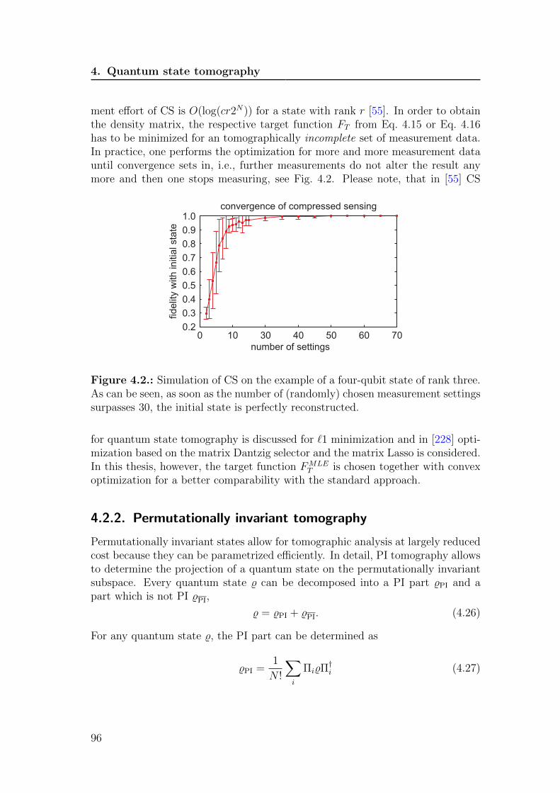
4. Quantum state tomography
ment effort of CS is O(log(cr2N)) for a state with rank r [55]. In order to obtainthe density matrix, the respective target function FT from Eq. 4.15 or Eq. 4.16has to be minimized for an tomographically incomplete set of measurement data.In practice, one performs the optimization for more and more measurement datauntil convergence sets in, i.e., further measurements do not alter the result anymore and then one stops measuring, see Fig. 4.2. Please note, that in [55] CS
Figure 4.2.: Simulation of CS on the example of a four-qubit state of rank three.As can be seen, as soon as the number of (randomly) chosen measurement settingssurpasses 30, the initial state is perfectly reconstructed.
for quantum state tomography is discussed for `1 minimization and in [228] opti-mization based on the matrix Dantzig selector and the matrix Lasso is considered.In this thesis, however, the target function FMLE
T is chosen together with convexoptimization for a better comparability with the standard approach.
4.2.2. Permutationally invariant tomography
Permutationally invariant states allow for tomographic analysis at largely reducedcost because they can be parametrized efficiently. In detail, PI tomography allowsto determine the projection of a quantum state on the permutationally invariantsubspace. Every quantum state % can be decomposed into a PI part %PI and apart which is not PI %PI,
% = %PI + %PI. (4.26)
For any quantum state %, the PI part can be determined as
%PI =1
N !
∑i
Πi%Π†i (4.27)
96

4.2. Partial tomography schemes
where the Πi are permutation operators for qubits. For many relevant quantumstates like GHZ states, W states or symmetric Dicke states, the non-permutatio-nally invariant part vanishes and thus, even in many experimental realizations,only determining %PI is a fairly good approximation to %. So far, determining %PIhas been theoretically discussed for spin systems in [273, 274] and experimentallyimplemented for polarized photons in a single mode optical fiber in [275–277].
In the following, two different efficient representations of %PI shall be discussedand how they can be exploited for tomographic analysis. The first one is basedon PI correlations, which allows for a simple derivation of the number of freeparameters. The second representation utilizes a block diagonalization of %PItogether with coarse graining, which proves to be advantageous especially formaximum likelihood and least squares fitting algorithms.
Formally, a PI correlation TPIi1,...,iN
is defined as
TPIi1,...,iN
= 〈σi1 ⊗ ...⊗ σiN 〉PI =1
N !
∑i
Tr[%Πi(σi1 ⊗ ...⊗ σiN )Π†i ]. (4.28)
This definition reflects the fact that for PI states, the result of a correlation mea-surement is independent under swapping of local measurements. A PI quantumstate is uniquely described by its PI correlations, also called generalized Blochvector. Thus, in order to determine the measurement effort, it is necessary tocount the number of PI correlations. Therefore, let us consider Fig. 4.3a) wherea simple scheme to count PI correlations on the example of four qubits is shown.There are three vertical red bars to separate the local settings σ0, σx, σy and σz.The horizontal black place holders left of the red bar 1 are filled up with σ0, theplace holders between the red bars 1 and 2 are filled up with σx, those betweenthe red bars 2 and 3 are filled up with σy, and, finally, those right of the red bar 3are filled up with σz. The PI correlation corresponding to this arrangement of redthe bars is shown beneath. A second example is shown in Fig. 4.3b). With thisscheme, one can easily count all PI correlations of an N -qubit state. The total
1 2 3
ZZZX X Y1 2 3
11
XsX s s sZ Z Z\PI Xs0 s s s0 X Y\PI
a) b)
Figure 4.3.: With a simple combinatorial argument, the number of parametersthat need to be determined for permutationally invariant tomography is
(N+3N
).
For details, see the main text.
number of PI correlations is given then by the number of possible distributions ofthe three red bars which is, as can easily be seen,
(N+3N
)= 1
6(N3+6N2+11N+6).
97
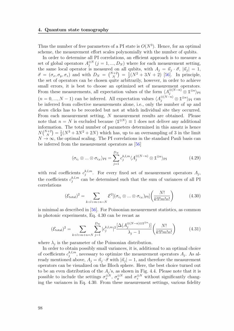
4. Quantum state tomography
Thus the number of free parameters of a PI state is O(N3). Hence, for an optimalscheme, the measurement effort scales polynomially with the number of qubits.
In order to determine all PI correlations, an efficient approach is to measure aset of global operators A⊗Nj (j = 1, ..., DN) where for each measurement setting,the same local operator is measured on all qubits, with Aj = ~nj · ~σ, |~nj| = 1,~σ = (σx, σy, σz) and with DN =
(N+2N
)= 1
2(N2 + 3N + 2) [56]. In principle,
the set of operators can be chosen quite arbitrarily, however, in order to achievesmall errors, it is best to choose an optimized set of measurement operators.From these measurements, all expectation values of the form 〈A⊗(N−n)j ⊗ 1⊗n〉PI(n = 0, ..., N − 1) can be inferred. All expectation values 〈A⊗(N−n)j ⊗ 1⊗n〉PI canbe inferred from collective measurements alone, i.e., only the number of up anddown clicks has to be recorded but not at which individual site they occurred.From each measurement setting, N measurement results are obtained. Pleasenote that n = N is excluded because 〈1⊗N〉 ≡ 1 does not deliver any additionalinformation. The total number of parameters determined in this ansatz is henceN(N+2N
)= 1
2(N3 + 3N2 + 2N) which has, up to an oversampling of 3 in the limit
N →∞, the optimal scaling. The PI correlations in the standard Pauli basis canbe inferred from the measurement operators as [56]
〈σi1 ⊗ ...⊗ σiN 〉PI =
DN∑j=1
ck,l,mj 〈A⊗(N−n)j ⊗ 1⊗n〉PI (4.29)
with real coefficients ck,l,mj . For every fixed set of measurement operators Aj,
the coefficients ck,l,mj can be determined such that the sum of variances of all PIcorrelations
(Etotal)2 =∑
k+l+m+n=N
E2[(σi1 ⊗ ...⊗ σiN )PI]
(N !
k!l!m!n!
)(4.30)
is minimal as described in [56]. For Poissonian measurement statistics, as commonin photonic experiments, Eq. 4.30 can be recast as
(Etotal)2 =∑
k+l+m+n=N
DN∑j=1
|ck,l,mj |2[∆(A
⊗(N−n)⊗1⊗n
j )]
λj − 1
(N !
k!l!m!n!
)(4.31)
where λj is the parameter of the Poissonian distribution.In order to obtain possibly small variances, it is, additional to an optimal choice
of coefficients ck,l,mj , necessary to optimize the measurement operators Aj. As al-ready mentioned above, Aj = ~nj ·~σ with |~nj| = 1, and therefore the measurementoperators can be visualized on the Bloch sphere. Here, the best choice turned outto be an even distribution of the Aj’s, as shown in Fig. 4.4. Please note that it ispossible to include the settings σ⊗Nx , σ⊗Ny and σ⊗Nz without significantly chang-ing the variances in Eq. 4.30. From these measurement settings, various fidelity
98

4.2. Partial tomography schemes
witnesses [278], entanglement witnesses [61, 158, 278, 279] and, more importantin this context, a lower bound for the overlap with the symmetric subspace canbe deduced [56].
1
0.5
0
-0.5
-1
aZ
10
-1 10
-1aX aY
1
0.5
0
-0.5
-1
aZ
10
-1 10
-1aX aY
a) b)
Figure 4.4.: Optimized set of measurement operators Aj visualized on the Blochsphere for a) four and b) six-qubit PI tomography.
Alternatively to the approach presented above, which is closely linked to theconcept of correlations, another ansatz based on a block diagonal decompositionof % and coarse graining exists. It is advantageous both with respect to linearinversion and a maximum likelihood reconstruction. As already mentioned, thePI part of a state % can be reconstructed from collective measurements alone.This property is reflected by the coarse grained measurement operators Mn
j [57]
Mnj =
∑i
Πi|0〉j〈0|⊗N−nj ⊗ |1〉j〈1|⊗N−nj Π†i (4.32)
=
(N
n
)[|0〉j〈0|⊗N−nj ⊗ |1〉j〈1|⊗N−nj
]PI
(4.33)
where Πi are permutation operators for qubits and |0〉j and |1〉j are the eigenvec-tors of Aj with eigenvalue +1 and −1, respectively. Using the expectation valuesof the coarse grained measurement operators, %PI can be expressed as a linearfunction of these expectation values in a similar way as in section 4.1.1. Moreprecisely, a basis of the PI subspace {Yn,PIj }, similar to the set {Yi} in Eq. 4.1,has to be found, such that %PI can be expressed as
%PI =
DN∑j=1
N∑n=1
Yn,PIj 〈Mnj 〉. (4.34)
Similar to section 4.1.1, a shorthand notation is introduced, Yn,PIj −→ YPIλ and
Mnj −→ Mλ. As explained, %PI is uniquely described by its PI correlations, here
labeled as TPIµ ,
%PI =1
2N
∑µ
TPIµ ΓPI
µ (4.35)
99

4. Quantum state tomography
with ΓPIµ the corresponding element of the symmetrized Pauli basis. Then the
expectation value pλ = 〈Mλ〉 can be determined as
pλ = Tr(%PIMλ) = Tr
(1
2N
∑µ
TPIµ ΓPI
µ Mλ
)=
1
2N
∑µ
Tr(MλΓPIµ )TPI
µ (4.36)
Similar to Eq. 4.7 in section 4.1.1, introducing matrix Bλ,µ = 12N
Tr(MλΓPIµ ), allows
to interpret Eq. 4.36 as a system of linear equations
~p = B~TPI. (4.37)
The further derivation of the basis elements YPIλ goes along the same line as in the
case of standard tomography discussed in section 4.1. Therefore, only the finalresult shall be given
YPIλ =
1
2N
∑µ
B−1µ,λΓPIµ . (4.38)
As already mentioned before, due to finite measurement statics, the probabilitiespλ can only be approximately determined in real experiments, i.e., fλ ≈ pλ, andthus
%PI =∑λ
YPIλ fλ. (4.39)
Note that the presented approach is simpler in the sense that it does not ne-cessitate to determine the coefficients ck,l,mj from Eq. 4.29. However, here, thedrawback is that there is no direct way as in Eq. 4.31 to quantify the expectederrors for a certain choice of measurement operators Aj. Nonetheless, as soon asa set of operators is proven to be appropriate in terms of the expected errors,Eq. 4.39 is a simple and straightforward way to infer the PI part of a quantumstate.
Apart from their usefulness for a direct evaluation of the PI part of a quantumstate, the coarse grained operators Mn
j are also beneficial for a scalable max-imum likelihood reconstruction of %PI. Permutationally invariant tomographydoes not only offer an efficient measurement scheme but also offers the possibilityto efficiently store and further process the obtained data on a digital computer.For this purpose, a basis change to the angular momentum basis is required.A possible choice of basis states for the N -qubit Hilbert space is |j, jz, α〉, with~J2|j, jz, α〉 = j(j+1)|j, jz, α〉, Jz|j, jz, α〉 = jz|j, jz, α〉. The total spin numbers arerestricted to j = jmin, jmin+1, ..., N
2starting from jmin = 0 for N even and jmin = 1
2
for N odd, while jz = −N2,−N
2+ 1, ..., N
2. Here, the label α was introduced to
remove the degeneracy of the eigenstates of ~J2 and J2z with degree dj [280]. In
this basis, any PI operator, like, e.g., %PI or Mnj , can be written in a simple block
diagonal form
%PI =
N/2⊕k=kmin
1dkdk⊗ pk%k (4.40)
100

4.2. Partial tomography schemes
with %k being the density operators of the spin-k subspace and pk a probabilitydistribution, see Fig. 4.5. Hence, as an equally efficient alternative to storing
Figure 4.5.: Every PI state allows for a block diagonal decomposition.
the generalized Bloch vector introduced in Eq. 4.28, it is also possible to storeonly the N
2blocks %j = pj%j/dj (of which each has a multiplicity of dj). The
largest of these blocks, which corresponds to the symmetric subspace, is of size(N+1)×(N+1) and multiplicity dN
2= 1. Thus, the block diagonal representation
of PI states is an efficient scheme for data storage. Moreover, as also the coarsegrained measurement operators Mn
k allow for a block diagonal representation,
Mnk =
N/2⊕j=jmin
1dk ⊗Mnk,j, (4.41)
expectation values of the kind Tr(%PIMnj ) can efficiently be calculated as follows
Tr(%PIMnj ) =
N/2∑k=kmin
pkTr(%kMnk,j). (4.42)
More precisely, in the standard representation the trace has to be taken over theproduct of two 2N -dimensional matrices, now there are only about N
2terms with
traces of at most (N + 1)-dimensional matrices. Again, the effort reduces fromexponential to polynomial. This speedup can be used beneficially to also makemaximum likelihood estimation scalable, i.e., the computational effort increasespolynomially with the system size. For details see publication P4.3.
Even if the state to be analyzed is not PI, as long as the observable to bemeasured is PI one can hugely benefit from the scheme thanks to the fact thata similarly scalable decomposition can be found for any PI operator O, i.e., O =⊕
j 1dj ⊗Oj. Together with Eq. (4.40) this yields an efficient way to calculate theexpectation values 〈O〉 = Tr(%O) =
∑j pjTr(%jOj) also for non-PI states. Please
note that if the operator whose expectation value is to be determined is PI, theresult obtained by means of permutationally invariant tomography is correct, evenin case the state under investigation is not PI.
101

4. Quantum state tomography
4.2.3. Compressed sensing in the permutationally invariantsubspace
In sections 4.2.1 and 4.2.2, two efficient tomography schemes were presented.The first one, CS, is suited for low rank states, i.e., states with only few non-zero eigenvalues. The second scheme, PI tomography, is ideal for the analysisof states that lie within the PI subspace. At this point, the question arises ifit is also possible to combine these two schemes as there are states that are atthe same time of low rank and PI. Prominent examples for such states are GHZstates and the symmetric Dicke states as discussed in this work. As expected, theanswer turns out to be positive. More precisely, in order to carry out CS in the PIsubspace, only a subset of the set of operators A⊗Nj (j = 1, ..., DN) is measured.Then, the target function 4.14 is minimized under the constraint of % being PI andpositive-semidefinite. This scheme is experimentally implemented in publicationP4.3 on the example of a symmetric six-photon Dicke state. There, it could beshown that CS in the PI subspace can further reduce the experimental withoutsignificantly changing the reconstructed state. For more details see publicationP4.2 and for a description of the fitting algorithm, see publication P4.3.
4.3. Publications
102

Permutationally Invariant Quantum Tomography
G. Toth,1,2,3 W. Wieczorek,4,5,* D. Gross,6 R. Krischek,4,5 C. Schwemmer,4,5 and H. Weinfurter4,5
1Department of Theoretical Physics, The University of the Basque Country, P.O. Box 644, E-48080 Bilbao, Spain2IKERBASQUE, Basque Foundation for Science, E-48011 Bilbao, Spain
3Research Institute for Solid State Physics and Optics, Hungarian Academy of Sciences, P.O. Box 49, H-1525 Budapest, Hungary4Max-Planck-Institut fur Quantenoptik, Hans-Kopfermann-Strasse 1, D-85748 Garching, Germany
5Fakultat fur Physik, Ludwig-Maximilians-Universitat, D-80797 Munchen, Germany6Institute for Theoretical Physics, Leibniz University Hannover, D-30167 Hannover, Germany
(Received 4 June 2010; revised manuscript received 30 August 2010; published 16 December 2010)
We present a scalable method for the tomography of large multiqubit quantum registers. It acquires
information about the permutationally invariant part of the density operator, which is a good approxi-
mation to the true state in many relevant cases. Our method gives the best measurement strategy to
minimize the experimental effort as well as the uncertainties of the reconstructed density matrix. We apply
our method to the experimental tomography of a photonic four-qubit symmetric Dicke state.
DOI: 10.1103/PhysRevLett.105.250403 PACS numbers: 03.65.Wj, 03.65.Ud, 42.50.Dv
Because of the rapid development of quantum experi-ments, it is now possible to create highly entangled multi-qubit states using photons [1–5], trapped ions [6], and coldatoms [7]. So far, the largest implementations that allowfor an individual readout of the particles involve on theorder of 10 qubits. This number will soon be overcome, forexample, by using several degrees of freedom within eachparticle to store quantum information [8]. Thus, a newregime will be reached in which a complete state tomog-raphy is impossible even from the point of view of thestorage place needed on a classical computer. At this pointthe question arises: Can we still extract useful informationabout the quantum state created?
In this Letter we propose permutationally invariant(PI) tomography in multiqubit quantum experiments [9].Concretely, instead of the density matrix %, we propose todetermine the PI part of the density matrix defined as
%PI ¼ 1
N!
Xk
�k%�k; (1)
where �k are all the permutations of the qubits.Reconstructing %PI has been considered theoretically forspin systems (see, e.g., Ref. [10]). Recently it has beenpointed out that photons in a single mode optical fiber willalways be in a PI state and that there is only a small set ofmeasurements needed for their characterization [11,12].
Here, we develop a provably optimal scheme, which isfeasible for large multiqubit systems: For our method, themeasurement effort increases only quadratically with thesize of the system. Our approach is further motivated bythe fact that almost allmultipartite experiments are donewithPI quantum states [2–4,6]. Thus, the density matrix obtainedfrom PI tomography is expected to be close to the one of theexperimentally achieved state. The expectation values ofsymmetric operators, such as some entanglement witnesses,and fidelities with respect to symmetric states are the same
for both density matrices and are thus obtained exactly fromPI tomography [2–4]. Finally, if %PI is entangled, so is thestate % of the system, which makes PI tomography a usefuland efficient tool for entanglement detection.Below, we summarize the four main contributions of this
Letter. We restrict our attention to the case of N qubits—higher-dimensional systems can be treated similarly.(1) In most experiments, the qubits can be individually
addressed whereas nonlocal quantities cannot be measureddirectly. The experimental effort is then characterized bythe number of local measurement settings needed, where‘‘setting’’ refers to the choice of one observable per qubit,and repeated von Neumann measurements in the observ-ables’ eigenbases [13]. Here, we compute the minimalnumber of measurement settings required to recover %PI.(2) The requirement that the number of settings be
minimal does not uniquely specify the tomographic proto-col. On the one hand, there are infinitely many possiblechoices for the local settings that are both minimal andgive sufficient information to find %PI. On the other hand,for each given setting, there are many ways of estimatingthe unknown density operator from the collected data. Wepresent a systematic method to find the optimal schemethrough statistical error analysis.(3) Next, we turn to the important problem of gauging
the information loss incurred due to restricting attention tothe PI part of the density matrix. We describe an easy testmeasurement that can be used to judge the applicability ofPI tomography before it is implemented.(4) Finally, we demonstrate that these techniques are
viable in practice by applying them to a photonic experi-ment observing a four-qubit symmetric Dicke state.Minimizing the number of settings.—We will now
present our first main result.Observation 1. For a system of N qubits, permuta-
tionally invariant tomography can be performed with
PRL 105, 250403 (2010) P HY S I CA L R EV I EW LE T T E R Sweek ending
17 DECEMBER 2010
0031-9007=10=105(25)=250403(4) 250403-1 � 2010 The American Physical Society
4.3. Publications
P4.1
103

D N ¼ N þ 2N
� �¼ 1
2ðN2 þ 3N þ 2Þ (2)
local settings. It is not possible to perform such a tomog-raphy with fewer settings.
Proof.—First, we need to understand the informationobtainable from a single measurement setting. We assumethat for every given setting, the same basis is measured atevery site [14]. Measuring a local basis fj�1i; j�2ig isequivalent to estimating the expectation value of the trace-less operator A ¼ j�1ih�1j � j�2ih�2j. Merely by mea-suring A�N , it is possible to obtain all the N expectationvalues
hðA�ðN�nÞ � 1�nÞPIi; ðn ¼ 0; . . . ; N � 1Þ; (3)
and, conversely, that is all the information obtainable about%PI from a single setting.
Next, we will use the fact that any PI density operatorcan be written as a linear combination of the pairwiseorthogonal operators ðX�k � Y�l � Z�m � 1�nÞPI, whereX, Y, and Z are the Pauli matrices. We consider the spacespanned by these operators for one specific value of n.Simple counting shows that its dimension is DðN�nÞ. Thesame space is spanned by DðN�nÞ generic operators of thetype ðA�ðN�nÞ � 1�nÞPI. We draw two conclusions: First,any setting gives at most one expectation value for everysuch space. Hence the number of settings cannot be smallerthan the largest dimension, which isDN . Second, a genericchoice of DN settings is sufficient to recover the correla-tions in each of these spaces, and hence completely char-acterizes %PI. This concludes the proof [15].
The proof implies that there are real coefficients cðk;l;mÞj
such that
hðX�k � Y�l � Z�m � 1�nÞPIi
¼ XDN
j¼1
cðk;l;mÞj hðA�ðN�nÞ
j � 1�nÞPIi: (4)
Wewill refer to the numbers on the left-hand side of Eq. (4)as the elements of the generalized Bloch vector. The ex-pectation values on the right-hand side can be obtained bymeasuring the settings with Aj for j ¼ 1; 2; . . . ;DN .
Minimizing uncertainties.—We now have to determinethe optimal scheme for PI tomography. To this end, wedefine our measure of statistical uncertainty as the sum ofthe variances of all the Bloch vector elements
ðEtotalÞ2 ¼X
kþlþmþn¼N
E2½ðX�k � Y�l � Z�m � 1�nÞPI�
��
N!
k!l!m!n!
�; (5)
where the term with the factorials is the number of differ-ent permutations of X�k � Y�l � Z�m � 1�n. Based onEq. (4), the variance of a single Bloch vector element is
E 2½ðX�k � Y�l � Z�m � 1�nÞPI�
¼ XDN
j¼1
jcðk;l;mÞj j2E2½ðA�ðN�nÞ
j � 1�nÞPI�: (6)
Equation (5) can be minimized by changing the Aj matrices
and the cðk;l;mÞj coefficients.We consider the coefficients first.
For any Bloch vector element, finding cðk;l;mÞj ’s thatminimize
the variance Eq. (6) subject to the constraint that equalityholds in Eq. (4) is a least squares problem. It has an analyticsolution obtained as follows: Write the operator on the left-hand side of Eq. (6) as a vector ~v (with respect to some basis).Likewise, write the operators on the right-hand side as ~vj and
define a matrix V¼½ ~v1; ~v2; .. . ; ~vDN�. Then Eq. (4) can be
cast into the form ~v ¼ V ~c, where ~c is a vector of the cðk;l;mÞj
values for given ðk; l; mÞ. If E is the diagonal matrix with en-
triesE2j;j ¼ E2½ðA�ðN�nÞ
j � 1�nÞPI�, then the optimal solution
is ~c ¼ E�2VTðVE�2VTÞ�1 ~v, where the inverse is taken overthe range [16].Equipped with a method for obtaining the optimal
cðk;l;mÞj ’s for every fixed set of observables Aj, it remains to
find the best settings tomeasure. Every qubit observable canbe defined by the measurement directions ~aj using Aj ¼aj;xX þ aj;yY þ aj;zZ. Thus, the task is to identify DN
measurement directions on the Bloch sphere minimizingthe variance. In general, finding the globally optimal solu-tion of high-dimensional problems is difficult. In our case,however, Etotal seems to penalize an inhomogeneous distri-bution of the ~aj vectors; thus, using evenly distributed vec-
tors as an initial guess, usual minimization procedures canbe used to decrease Etotal and obtain satisfactory results [16].
The variance E2½ðA�ðN�nÞj � 1�nÞPI� of the observed
quantities depends on the physical implementation. In thephotonic setup below, we assume Poissonian distributedcounts. It follows that (see also Refs. [17,18])
E 2½ðA�ðN�nÞj � 1�nÞPI� ¼
½�ðA�ðN�nÞj � 1�nÞPI�2%0
�j � 1; (7)
where ð�AÞ2% ¼ hA2i% � hAi2%, %0 is the state of the system,
and �j is the parameter of the Poissonian distribution,
which equals the expected value of the total number ofcounts for the setting j. The variance depends on the un-known state. If we have preliminary knowledge of thelikely form of %0, we should use that information in theoptimization. Otherwise, %0 can be set to the completelymixed state. For the latter, straightforward calculation
shows that E2½ðA�ðN�nÞj � 1�nÞPI� ¼ ðNnÞ�1=ð�j � 1Þ. For
another implementation, such as trapped ions, our schemefor PI tomography can be used after replacing Eq. (7) bya formula giving the variance for that implementation.Estimating the information loss due to symmetriza-
tion.—It is important to know how close the PI quantumstate is to the state of the system as PI tomography should
PRL 105, 250403 (2010) P HY S I CA L R EV I EW LE T T E R Sweek ending
17 DECEMBER 2010
250403-2
4. Quantum state tomography
104

serve as an alternative of full state tomography for experi-ments aiming at the preparation of PI states.
Observation 2. The fidelity between the original stateand the permutationally invariant state, Fð%; %PIÞ, can
be estimated from below as Fð%; %PIÞ � hPsi2%, where Ps ¼PNn¼0 jDðnÞ
N ihDðnÞN j is the projector to the N-qubit symmetric
subspace, and the symmetric Dicke state is defined as
jDðnÞN i ¼ ðNnÞ�1=2
PkP kðj0i�ðN�nÞ � j1i�nÞ, where the sum-
mation is over all the different permutations of the qubits.Observation 2 can be proved based on Ref. [19] and elemen-tary matrix manipulations. Note that Observation 2 makesit possible to estimate Fð%; %PIÞ based on knowing only %PI.
Lower bounds on the fidelity to symmetric Dicke states,
i.e., TrðjDðnÞN ihDðnÞ
N j%Þ can efficiently be obtained by mea-suring X, Y, and Z on all qubits, i.e., measuring only threelocal settings independent of N [20]. With the samemeasurements, one can also obtain a lower bound on theoverlap between the state and the symmetric subspace.For four qubits, this can be done based on Ps � ½ðJ4x þJ4y þ J4z Þ � ðJ2x þ J2y þ J2z Þ�=18, where Jx ¼ ð1=2ÞPkXk,
Jy ¼ ð1=2ÞPkYk, etc. Operators for estimating hPsi for
N ¼ 6; 8 are given in Ref. [16]. This allows one to judgehow suitable the quantum state is for PI tomography beforesuch a tomography is carried out.
Experimental results.—We demonstrate the method andthe benefits of our algorithm for PI tomography for a four-
qubit symmetric Dicke state with two excitations jDð2Þ4 i.
First, we optimize the ~aj’s and the cðk;l;mÞj ’s for %0 ¼ 1=16
and only for the uncertainty of full four-qubit correlationterms, which means that when computing Etotal, we carry outthe summation in Eq. (5) only for the termswith n ¼ 0. Withsimple numerical optimization,wewere looking for the set ofAj basis matrices that minimize the uncertainty of the full
correlation terms. Then,we also looked for the basismatricesthat minimize the sum of the squared error of all the Blochvector elements and considered also density matrices differ-ent from white noise, such as a pure Dicke state mixed withnoise. We find that the gain in terms of decreasing theuncertainties is negligible in our case and that it is sufficientto optimize for %0 ¼ 1=16 and for the full correlation terms.To demonstrate the benefits of the optimization of the mea-surement directions, we also compare the results with thoseobtained with randomly distributed basis matrices.
The Dicke state was observed in a photonic system.Essentially, four photons emitted by the second-order col-linear type-II spontaneous parametric down-conversionprocess were symmetrically distributed into four spatialmodes. Upon detection of one photon from each of the
outputs, the state jDð2Þ4 i is observed. Polarization analysis
in each mode is used to characterize the experimentallyobserved state. We collected data for each setting for 5 min,with an average count rate of 410 per minute. The experi-mental setup has been described in detail in Refs. [2,3].
First, to check the applicability of the PI tomography,we apply our tools described above requiring only the
measurement of the three settings, X�4, Y�4, and Z�4.We determine the expectation value of the projector tothe symmetric subspace, yielding hPsi � 0:905� 0:015.Based on Observation 2, we obtain Fð%; %PIÞ � 0:819�0:028. These results show that the state is close to be PIand has a large overlap with the symmetric subspace. Thus,it makes sense to apply PI tomography.For PI tomography of a four-qubit system, the measure-
ment of 15 settings is needed. We used Eq. (4) to obtain theBloch vector elements from the experimentally measuredquantities. This way, we could obtain all the 34 symmetriccorrelations of the form ðX�k � Y�l � Z�m � 1�nÞPI. InFig. 1, we give the values of the correlations for optimizedand for randomly chosen measurement directions, com-pared to the results obtained from full tomography, whichneeded 81 measurement settings. As can be seen in Fig. 1,the uncertainty for the optimized settings is considerablysmaller than the one for the randomly chosen settings.Moreover, the results from the optimized settings fit verywell the results of the full tomography. In Fig. 2, wecompare the density matrices obtained from full tomogra-phy [Fig. 2(a)], from PI tomography for optimized[Fig. 2(b)], and for random measurement directions[Fig. 2(c)]. Because of noise, the fidelity of the result of
the full tomography with respect to jDð2Þ4 i is 0:873� 0:005,
which is similar to the fidelity of the results of the PItomography with optimized settings, 0:852� 0:009 [21].In contrast, for the method using random measurementdirections, the fidelity is 0:814� 0:059, for which the
−1
−0.5
0
0.5
1
Sym
. cor
rela
tion
X X X X Y X X X Y X X Y X Y Z X X X Y X X Y X Y Z X X Y X Y Z X Y Z
X X X Y Y X X Y Y X Y Y Z Z Z X X Y Y X Y Y Z Z Z X Y Y Z Z Z 1 1 1
X X Y Y Y X Y Y Y Z Z Z Z Z Z X Y Y Y Z Z Z Z Z Z 1 1 1 1 1 1 1 1 1
X Y Y Y Y Z Z Z Z Z Z Z Z Z Z 1 1 1 1 1 1 1 1 1 1 1 1 1 1 1 1 1 1 1
(a)
PI tomogrpahy withoptimized settings vs.full tomogrpahy
−10
1 −10
1
−1
−0.5
0
0.5
1
aya
x
a z
(b)
−1
−0.5
0
0.5
1
Sym
. cor
rela
tion
X X X X Y X X X Y X X Y X Y Z X X X Y X X Y X Y Z X X Y X Y Z X Y Z X X X Y Y X X Y Y X Y Y Z Z Z X X Y Y X Y Y Z Z Z X Y Y Z Z Z 1 1 1
X X Y Y Y X Y Y Y Z Z Z Z Z Z X Y Y Y Z Z Z Z Z Z 1 1 1 1 1 1 1 1 1
X Y Y Y Y Z Z Z Z Z Z Z Z Z Z 1 1 1 1 1 1 1 1 1 1 1 1 1 1 1 1 1 1 1
(c)
PI tomogrpahy withrandom settings vs.full tomogrpahy
−10
1 −10
1
−1
−0.5
0
0.5
1
aya
x
a z
(d)
FIG. 1 (color online). (a) Comparison of the 34 symmetrizedcorrelations coming from (crosses with error bars) 15 permutation-ally invariant measurement settings with optimized Aj matrices for
N ¼ 4 qubits and (diamonds) from full tomography requiring 81local settings. The average uncertainty of all symmetrized correla-tions obtained from full tomography is�0:022, and is not shown inthe figure. The labels refer to symmetrized correlations of the formgiven in the left-hand side of Eq. (4). The results corresponding tothe 15 full four-qubit correlations are left from the vertical dashedline. (b)Measurement directions.A point at ðax; ay; azÞ correspondsto measuring operator axX þ ayY þ azZ. (c) Results for randomly
chosen Aj matrices and (d) corresponding measurement directions.
PRL 105, 250403 (2010) P HY S I CA L R EV I EW LE T T E R Sweek ending
17 DECEMBER 2010
250403-3
4.3. Publications
105

uncertainty is the largest compared to all previous fidelityvalues. Finally, we also computed the fidelity of the resultswith respect to the PI density matrix obtained from fulltomography [22]. The results of the PI tomography withoptimized settings show a good agreement with full to-mography: the fidelity is 0.947, which is quite close to thefidelity between the results of full tomography and its PIpart, 0.964. On the other hand, for the PI tomography withrandom settings the corresponding fidelity is much lower,0.880. Overall, the PI tomography shows a good agreementwith the full tomography for this particular experiment.However, a reasonable choice of measurement directions isneeded to obtain uncertainties in the reconstructed Blochvector elements similar to the ones from full tomography.
Finally, let us comment on how our method can be ex-tended to lager systems. Permutationally invariant operatorscan be represented efficiently on a digital computer in thebasis of ðX�k�Y�l�Z�m�1�nÞPI operators.Wedeterminedthe optimal Aj operators for PI tomography for systems with
N ¼ 6; 8; . . . ; 14 qubits. To have the same maximum uncer-tainty of theBlochvector elements as for theN ¼ 4 case, onehas to increase the counts per setting by less than 50% [16].
In summary, we presented a scalablemethod for permuta-tionally invariant tomography, which can be used in place offull state tomography in experiments that aim at preparingpermutationally invariant many-qubit states. For our ap-proach, the same operator has to be measured on all qubits,
which is a clear advantage in some experiments.We showedhow to choose themeasurements such that the uncertainty inthe reconstructed density matrix is the smallest possible.This paves the way of characterizing permutationally in-variant states of many qubits in various physical systems.Moreover, this work also shows that, given some knowledgeor justifiable assumptions, there is a way to obtain scalablestate tomography for multiqubit entangled states.We thank D. Hayes and N. Kiesel for discussions. We
thank the Spanish MEC (Consolider-Ingenio 2010 project’’QOIT,’’ Project No. FIS2009-12773-C02-02), the BasqueGovernment (Project No. IT4720-10), the ERC StGGEDENTQOPT, the DFG-Cluster of Excellence MAP,the EU projects QAP, Q-Essence, and CORNER, and theDAAD/MNISW for support. W.W. and C. S. thank theQCCC of the Elite Network of Bavaria for support.
*Present address: Faculty of Physics, University of Vienna,Boltzmanngasse 5, A-1090 Wien, Austria.
[1] J.-W. Pan et al., Nature (London) 403, 515 (2000);M. Bourennane et al., Phys. Rev. Lett. 92, 087902(2004); N. Kiesel et al., ibid. 95, 210502 (2005).
[2] N. Kiesel et al., Phys. Rev. Lett. 98, 063604 (2007).[3] W. Wieczorek et al., Phys. Rev. Lett. 103, 020504 (2009);
R. Krischek et al., Nat. Photon. 4, 170 (2010).[4] R. Prevedel et al., Phys. Rev. Lett. 103, 020503 (2009).[5] W. Wieczorek et al., Phys. Rev. Lett. 101, 010503 (2008).[6] C. A. Sackett et al., Nature (London) 404, 256 (2000);
H. Haffner et al., Nature (London) 438, 643 (2005).[7] O. Mandel et al., Nature (London) 425, 937 (2003).[8] C. Cinelli et al., Phys. Rev. Lett. 95, 240405 (2005);
G. Vallone et al., ibid. 98, 180502 (2007); W.-B. Gaoet al., Nature Phys. 6, 331 (2010).
[9] For other approaches see D. Gross et al., Phys. Rev. Lett.105, 150401 (2010); M. Cramer and M. B. Plenio,arXiv:1002.3780; S. T. Flammia et al., arXiv:1002.3839;O. Landon-Cardinal et al., arXiv:1002.4632.
[10] G.M. D’Ariano et al., J. Opt. B 5, 77 (2003).[11] R. B. A.Adamson et al., Phys. Rev. Lett. 98, 043601 (2007).[12] L. K. Shalm et al., Nature (London) 457, 67 (2009).[13] O. Guhne and G. Toth, Phys. Rep. 474, 1 (2009).[14] Otherwise more than DN settings are necessary [16].[15] This is connected to a general idea: It is expected that the
determination of an operator within a subspace whosedimension depends polynomially on N needs a numberof settings increasing also polynomially with N.
[16] See supplementary material at http://link.aps.org/supplemental/10.1103/PhysRevLett.105.250403 for addi-tional derivations and experimental results.
[17] C. Schmid, Ph.D. thesis, Ludwig-Maximillian-Universitat,2008; D. F. V. James et al., Phys. Rev. A 64, 052312 (2001).
[18] B. Jungnitsch et al., Phys. Rev. Lett. 104, 210401 (2010).[19] J. A.Miszczak et al., Quantum Inf. Comput. 9, 0103 (2009).[20] G. Toth et al., New J. Phys. 11, 083002 (2009).[21] Expectation values are obtained directly from the mea-
sured data, rather than from �PI.[22] Values without error are deduced from fitted matrices
obtained via maximum likelihood estimation [17].
FIG. 2 (color online). (a) The real and (b) imaginary parts ofthe density matrix coming from full tomography. (c),(d) Thesame for permutationally invariant tomography with optimizedand (e),(f) random measurement directions, respectively.
PRL 105, 250403 (2010) P HY S I CA L R EV I EW LE T T E R Sweek ending
17 DECEMBER 2010
250403-4
4. Quantum state tomography
106

Permutationally Invariant Quantum Tomography - Supplementary Material
Géza Tóth,1, 2, 3 Witlef Wieczorek,4, 5, ∗ David Gross,6 Roland Krischek,4, 5 Christian Schwemmer,4, 5 and Harald Weinfurter4, 5
1Department of Theoretical Physics, The University of the Basque Country, P.O. Box 644, E-48080 Bilbao, Spain2IKERBASQUE, Basque Foundation for Science, E-48011 Bilbao, Spain
3Research Institute for Solid State Physics and Optics,Hungarian Academy of Sciences, P.O. Box 49, H-1525 Budapest, Hungary
4Max-Planck-Institut für Quantenoptik, Hans-Kopfermann-Strasse 1, D-85748 Garching, Germany5Fakultät für Physik, Ludwig-Maximilians-Universität, D-80797 München, Germany
6Institute for Theoretical Physics, Leibniz University Hannover, D-30167 Hannover, Germany(Dated: December 23, 2010)
The supplement contains some derivations to help to understand the details of the proofs of the main text. Italso contains some additional experimental results.
PACS numbers: 03.65.Wj, 42.50.Dv, 03.65.Ud
Proof of that we have to measure the same operator on allqubits. From the proof of Observation 1, we know that at leastDN measurements are needed to get the expectation valuesof all the DN independent symmetric full N -particle correla-tions. What if we measure DN settings, but several of themare not {Aj , Aj , ..., Aj}-type, but {A(1)
j , A(2)j , ..., A
(N)j }-
type, i.e., we do not measure the same operator on all qubits?Each setting makes it possible to get a single operator con-taining full N -qubit correlations. Let us denote this operatorby Mk for k = 1, 2, ...,DN . Then, we know the expectationvalue of any operator of the space defined by the Mk oper-ators. However, not all Mk’s are permutationally invariant.Thus, the size of the PI subspace of the space of the Mk opera-tors is less than DN . We do not have DN linearly independentsymmetric operators in this space. Thus, DN measurementsettings are sufficient to measure ϱPI only if we have settingsof the type {Aj , Aj , ..., Aj}.
Derivation of Eq. (7). The eigen-decomposition of the cor-relation term is
(A⊗(N−n)j ⊗ 11⊗n)PI =
∑k
Λj,n,k|Φj,k⟩⟨Φj,k|. (S1)
The individual counts NC(Aj)k follow a Poissonian distribu-tion f(nc, λj,k), where λj,k are the parameters of the Poisso-nian distributions and
∑k λj,k = λj . The conditional vari-
ance, knowing that the total count is NC(Aj), is
E2[(A⊗(N−n)j ⊗11⊗n)PI|NC(Aj)] =
[∆(A⊗(N−n)j ⊗ 11⊗n)PI]
2
NC(Aj).
(S2)After straightforward algebra, the variance is obtained as
E2[(A⊗(N−n)j ⊗ 11⊗n)PI]
=∑m
f(m,λj)E2[(A⊗(N−n)j ⊗ 11⊗n)PI|NC(Aj) = m]
=[∆(A
⊗(N−n)j ⊗ 11⊗n)PI]
2
λj − 1. (S3)
Similar results can be obtained through assuming Poisso-nian measurement statistics and Gaussian error propagation
[S1, S2]. If ϱ0 = 11/2N , then ∆(A⊗(N−n)j ⊗ 11⊗n)PI is in-
dependent from the choice of Aj . By substituting Aj = Z,straightforward calculations gives
E2[(A⊗(N−n)j ⊗ 11⊗n)PI] =
(Nn
)−1
λj − 1. (S4)
Obtaining the formula for c(k,l,m)j for the smallest error.
We look for c(k,l,m)j for which the squared uncertainty given in
Eq. (6) is the smallest. In the following, we use the definitiongiven in the main text for c, v, V and E. Thus, V is matrixmapping a large space Rl to a small space Rs. Let E be anon-singular diagonal matrix in the small space. We have tosolve
minc
∥Ec∥2 s.t. V c = v, (S5)
where ||a|| is the Euclidean norm of a. Using Lagrangian mul-tipliers, we write down the condition for a minimum fulfillingthe constraints V c = v
∇c
{cTE2c+
s∑i=1
λi
[(V c)i − wi
]}= 0. (S6)
Hence, the condition for a local (and, due to convexity, global)minimum is
c =1
2E−2V T λ, (S7)
where λ ∈ Rs is the vector of multipliers. In other words, wehave a minimum if and only if c ∈ rangeE−2V T . Becausethe range of V T is an s-dimensional subspace in Rl, there isa unique c in that range such that V c = v. A solution in aclosed form can be obtained as
c = E−2V T (V E−2V T )−1v. (S8)
Simple calculation shows that the V c = v condition holds
V c = V E−2V T (V E−2V T )−1v = v. (S9)
4.3. Publications
107

2
Table S1: Fidelities to the 4-qubit Dicke states.
measurement |D(0)4 ⟩ |D(1)
4 ⟩ |D(2)4 ⟩ |D(3)
4 ⟩ |D(4)4 ⟩ Σ
full tomography −0.001± 0.002 0.023± 0.004 0.873± 0.005 0.026± 0.004 0.002± 0.002 0.922
full tomography (max-like) 0.001 0.021 0.869 0.023 0 0.914
PI tomography −0.001± 0.002 0.040± 0.007 0.852± 0.009 0.036± 0.007 −0.002± 0.002 0.925
PI tomography (max-like) 0.003 0.038 0.850 0.037 0 0.928
PI tomography (ran) 0.000± 0.002 0.055± 0.027 0.814± 0.059 0.023± 0.027 0.001± 0.002 0.893
PI tomography (ran,max-like) 0.004 0.050 0.816 0.020 0.007 0.897
Proof of Observation 2. The eigenstates of J2 = J2x +
J2y+J2
z are usually labelled by |j,m, α⟩, where J2|j,m, α⟩ =j(j + 1)|j,m, α⟩, Jz|j,m, α⟩ = m|j,m, α⟩, and α is used tolabel the different eigenstates having the same j and m [S3].Let Pj,α denote the projector to the subspace of a given j andα. The number of subspaces is denoted by NSS, and, for agiven N , it can be calculated from group theory. Moreover,Ps ≡ PN/2,1. Using this notation, ϱPI =
∑j,α Pj,αϱPj,α =
(PsϱPs) +∑
j<N/2,α(Pj,αϱPj,α). In the basis of J2 eigen-states, ϱPI can be written as a block diagonal matrix
ϱPI =⊕j,α
(⟨Pj,α⟩ϱϱj,α) , (S10)
where ϱj,α are density matrices of size (2j + 1) × (2j + 1).In another context,
ϱPI =∑j,α
⟨Pj,α⟩ϱϱj,α, (S11)
where ϱj,α = Pj,αϱPj,α/Tr(Pj,αϱPj,α). Based on that, weobtain
F (ϱ, ϱj,α) = ⟨Pj,α⟩ϱ. (S12)
Then, due to the separate concavity of the fidelity, i.e.,F (ϱ, p1ϱ1 + p2ϱ2) ≥ p1F (ϱ, ϱ1) + p2F (ϱ, ϱ2), we obtainF (ϱ, ϱPI) ≥ ⟨Ps⟩ϱF (ϱ, ϱs) +
∑j<N/2,α⟨Pj,α⟩ϱF (ϱ, ϱj,α).
Substituting Eq. (S12) into this inequality, we obtainF (ϱ, ϱPI) ≥ ⟨Ps⟩2ϱ +
∑j<N/2,α⟨Pj,α⟩2ϱ. Using the fact that
⟨Ps⟩ϱ +∑
j<N/2,α⟨Pj,α⟩ϱ = 1, we obtain
F (ϱ, ϱPI) ≥ ⟨Ps⟩2ϱ +(1− ⟨Ps⟩ϱ)2
NSS − 1. (S13)
In many practical situations, the state ϱ is almost symmetricand N is large. In such cases the second term in Eq. (S13)is negligible. Thus, a somewhat weaker bound presented inObservation 2 can be used.
Numerical optimization used to minimize Etotal. Themeasurement directions minimizing Etotal can be obtained asfollows. Let us represent the measurement directions by three-dimensional vectors {aj}DN
j=1. The operators can be obtainedas Aj = aj,xX + aj,yY + aj,zZ.
First, we need an initial guess. This can come from a setof randomly chosen vectors representing the measurement di-rections. One can also use the result of a minimization for
Figure S1: (a) The difference of the real part of the density matri-ces from optimized settings and the one of full tomography. (b) Thedifference of the density matrices from random settings and the oneof full tomography. For the former, no clear structure is observed,whereas for the latter the largest difference is observed for the antidi-agonal elements.
some measure that characterizes how equally the vectors aredistributed. Such a measure is defined by
F({vj}) =∑k,l
(vk · vl)2m, (S14)
where vk represent the measurement directions and · is thescalar product and m is an integer. Such cost functions, calledframe potentials, appear in the theory of t-designs essentiallyfor the same purpose.
After we obtain the initial guess from such a procedure,we start an optimization for decreasing Etotal. At each itera-tion of the method, we change the measurement directions byrotating them with a small random angle around a randomlychosen axis. If the change decreases Etotal, then we keep thenew measurement directions, while if it does not then we dis-card it. We repeat this procedure until Etotal does not changesignificantly.
Three-setting witness for estimating the fidelity Thethree-setting witness for detecting genuine multipartite entan-glement in the vicinity of the Dicke state is [S4]
W(P3)D(4,2) = 2·11+ 1
6 (J2x+J2
y−J4x−J4
y )+3112J
2z− 7
12J4z . (S15)
For this witness we have [S4]
W(P3)D(4,2) − 3W(P)
D(4,2) ≥ 0, (S16)
4. Quantum state tomography
108

3
4 6 8 10 12 140
0.005
0.01
0.015
0.02
0.025
N
ε max
Figure S2: The maximum uncertainty of the Bloch vector elementsdefined in Eq. (S21) for the optimal measurement settings as a func-tion of the number of qubits, N, for N = 4, 6, 8, 10, 12 and 14.
where the projector witness is defined as
W(P)D(4,2) =
23 · 11 − |D(2)
4 ⟩⟨D(2)4 |. (S17)
Hence, the fidelity with respect to the state |D(2)4 ⟩ is bounded
from below as [S4]
FD(4,2) ≥ 23 − 1
3 ⟨W(P3)D(4,2)⟩. (S18)
Fidelities with respect to the four-qubit Dicke states. InTable S1 we summarize the results for full tomography (full)and for permutationally invariant tomography (pi) for random(ran) and optimized (opt) directions. To obtain a physicaldensity matrix with non-negative eigenvalues we perform amaximum-likelihood fit (max-like) of the measured data. InFig. S1, the differences between the density matrix obtainedfrom full tomography and the ones obtained from permuta-tionally invariant tomography can be seen.
Efficient representation of permutationally invariantoperators on a digital computer. Every PI operator O canbe decomposed as
O =∑
k+l+m+n=N
c(O)k,l,m,n(X
⊗k ⊗ Y ⊗l ⊗ Z⊗m ⊗ 11⊗n)PI.
(S19)Such a decomposition for operators of the form (A⊗(N−n) ⊗11⊗n)PI with A = axX + ayY + azZ is given by∑k,l,m
akxalya
mz
(k + l +m)!
k!l!m!(X⊗k ⊗ Y ⊗l ⊗ Z⊗m ⊗ 11⊗n)PI,
(S20)where the summation is carried out such that k+ l+m+n =N.
Results for larger systems. We determined the optimal Aj
for PI tomography for N = 4, 6, ..., 14. In Fig. S2, we plot themaximal uncertainty of the Bloch vector elements
ϵmax = maxk,l,m,n
E [(X⊗k ⊗ Y ⊗l ⊗ Z⊗m ⊗ 11⊗n)PI] (S21)
for the total count realized in the experiment λj = λ = 2050as a function of N, when the state of the system is ϱ0 = 11/2N .It increases slowly with N. Thus, for large N the number of
counts per measurement setting does not have to increase verymuch in order to keep the maximal uncertainty of the Blochvector elements the same as for the N = 4 case. In particular,for N = 14, a total count of 2797 per setting yields the samemaximal uncertainty as we had for the N = 4 case.
An upper bound on the uncertainty of PI tomography forϱ0 different from the white noise can be obtained by using[∆(A
⊗(N−n)j ⊗11⊗n)PI]
2ϱ0
= 1 for error calculations. Accord-ing to numerics, for optimal Aj for N = 4, 6, ..., 14, ϵmax re-mains the same as in the case of white noise, since for the fullcorrelation terms with n = 0 the upper bound equals the valuefor white noise, and the full correlations terms contribute tothe noise of the Bloch vector elements with the largest uncer-tainty. Thus, the total count per setting will not increase morewith the number of qubits even for states different from thecompletely mixed state.
The operators that give a bound on ⟨Ps⟩ with three settingsfor N = 6 and 8 are the following
P (6)s ≥ 2
225 (Q2 + J2z )− 1
90 (Q4 + J4z ) +
1450 (Q6 + J6
z ),
P (8)s ≥ −0.001616Q2 + 0.002200Q4 − 0.0006286Q6
+ 0.00004490Q8 + 0.003265J2z − 0.004444J4
z
+ 0.001270J6z − 0.00009070J8
z , (S22)
where Qn = Jnx + Jn
y . They were determined using semi-definite programming, with a method similar to one used forobtaining three-setting witnesses in Ref. [S4]. They have anexpectation value +1 for the Dicke states |D(3)
6 ⟩ and |D(4)8 ⟩,
respectively. Moreover, their expectation value give the high-est possible lower bound on ⟨Ps⟩ for states of the form
ϱnoisy(p) = p112N
+ (1− p)|D(N/2)N ⟩⟨D(N/2)
N | (S23)
among the operators that are constructed as a linear combi-nation of the operators Jn
l . The validity of the relations inEq. (S22) can easily be checked by direct calculation.
Bounding the differences between elements of ϱ and ϱPI
based on the fidelity. For any pure state |Ψ⟩, it is possible tobound the difference between |⟨Ψ|ϱPI|Ψ⟩| and |⟨Ψ|ϱ|Ψ⟩| as
|⟨Ψ|ϱ|Ψ⟩ − ⟨Ψ|ϱPI|Ψ⟩| ≤√1− F (ϱ, ϱPI). (S24)
Thus, if the fidelity is close to 1, then ⟨Ψ|ϱ|Ψ⟩ ≈ ⟨Ψ|ϱPI|Ψ⟩,even if |Ψ⟩ is non-symmetric. If |Ψ⟩ is an element of the prod-uct basis, e.g., |0011 ⟩, then Eq. (S24) is a bound on the dif-ference between the corresponding diagonal elements of ϱ andϱPI.
Eq. (S24) can be proved as follows: There is a well-knownrelation between the trace norm and the fidelity [S5]
1
2||ϱ− ϱPI||tr ≤
√1− F (ϱ, ϱPI). (S25)
Moreover, for a projector P and density matrices ϱk we have[S6]
|Tr(Pϱ1)− Tr(Pϱ2)| ≤1
2||ϱ1 − ϱ2||tr. (S26)
4.3. Publications
109

4
Combining Eq. (S25) and Eq. (S26), leads to Eq. (S24).
∗ Present address: Faculty of Physics, University of Vienna, Boltz-manngasse 5, A-1090 Wien, Austria
[S1] C. Schmid, Ph.D. Thesis, Ludwig-Maximillian-Universität,Munich, Germany, 2008; D.F.V. James et. al, Phys. Rev. A 64,
052312 (2001).[S2] B. Jungnitsch et. al, Phys. Rev. Lett. 104, 210401 (2010).[S3] See, for example, J.I. Cirac et. al, Phys. Rev. Lett. 82, 4344
(1999).[S4] G. Tóth et al., New J. Phys. 11, 083002 (2009).[S5] J.A. Miszczak et al., J. Quant. Inf. Comp. 9, 0103 (2009).[S6] See Eqs. (9.18) and (9.22) of M.A. Nielsen and I.L. Chuang,
Quantum computation and quantum information (CambridgeUniversity Press, Cambridge, 2000).
4. Quantum state tomography
110

Experimental Comparison of Efficient Tomography Schemes for a Six-Qubit State
Christian Schwemmer,1,2 Géza Tóth,3,4,5 Alexander Niggebaum,6
Tobias Moroder,7 David Gross,8 Otfried Gühne,7 and Harald Weinfurter1,21Max-Planck-Institut für Quantenoptik, Hans-Kopfermann-Straße 1, D-85748 Garching, Germany
2Department für Physik, Ludwig-Maximilians-Universität, D-80797 München, Germany3Department of Theoretical Physics, University of the Basque Country UPV/EHU, P.O. Box 644, E-48080 Bilbao, Spain
4IKERBASQUE, Basque Foundation for Science, E-48011 Bilbao, Spain5Wigner Research Centre for Physics, Hungarian Academy of Sciences, P.O. Box 49, H-1525 Budapest, Hungary
6School of Physics and Astronomy, University of Birmingham, B15 2TT Birmingham, United Kingdom7Naturwissenschaftlich-Technische Fakultät, Universität Siegen, Walter-Flex-Straße 3, D-57068 Siegen, Germany
8Physikalisches Institut & FDM, Universität Freiburg, Rheinstraße 10, D-79104 Freiburg, Germany(Received 29 January 2014; published 24 July 2014)
Quantum state tomography suffers from the measurement effort increasing exponentially with thenumber of qubits. Here, we demonstrate permutationally invariant tomography for which, contrary toconventional tomography, all resources scale polynomially with the number of qubits both in terms of themeasurement effort as well as the computational power needed to process and store the recorded data. Wedemonstrate the benefits of combining permutationally invariant tomography with compressed sensing bystudying the influence of the pump power on the noise present in a six-qubit symmetric Dicke state, a casewhere full tomography is possible only for very high pump powers.
DOI: 10.1103/PhysRevLett.113.040503 PACS numbers: 03.67.Mn, 03.65.Wj, 42.50.Dv
Introduction.—The number of controllable qubits inquantum experiments is steadily growing [1,2]. Yet, to fullycharacterize a multiqubit state via quantum state tomography(QST), the measurement effort scales exponentially with thenumber of qubits. Moreover, the amount of data to be savedand the resources to process them scale exponentially, too.Thus, the limit of conventional QST will soon be reached.The following question arises: how much information abouta quantum state can be inferred without all the measurementsa full QST would require? Protocols have been proposedwhich need significantly fewer measurement settings if onehas additional knowledge about a state, e.g., that it is of lowrank, a matrix product state, or a permutationally invariant(PI) state [3–8]. Some of these approaches only require apolynomially increasing number of measurements and evenoffer scalable postprocessing algorithms [5,8]. Yet, it isimportant to test the different approaches and evaluate theirresults for various quantum states.Here, we implement and compare four different QST
schemes in a six-photon experiment. In detail, we performthe largest QST of a photonic multiqubit state so far. Weuse these data as a reference for a detailed evaluation ofdifferent tomography schemes, which enable the statedetermination with significantly fewer measurements.The recently proposed, scalable PI analysis is implemented
here and thus enables us, for the first time, to also performthe numerical evaluation with polynomial resources only.We evaluate the convergence of compressed sensing (CS)schemes and show that the combination of PI and CS canfurther reduce the measurement effort, without sacrificingperformance. We demonstrate the usability of these sig-nificantly improved methods to characterize the effects ofhigher-order emission in spontaneous parametric down-conversion (SPDC), an analysis which would not have beenpossible without the novel tomography schemes.Scalable scheme for measurements.—Let us first con-
sider the measurement effort needed for tomography. For fullQST, each N-qubit state is associated with a normalizednon-negative Hermitian matrix ϱ with 4N − 1 real freeparameters. Since all free parameters have to be determined,any scheme that is suitable to fully analyzing an arbitrarystate, such as, e.g., the standard Pauli tomography scheme,suffers from an exponentially increasing measurement effort[9,10]. PI states, in contrast, are described by only�N þ 3
N
�− 1 ¼ OðN3Þ free parameters. Tomography in
the PI subspace can be performed by measuring (global)operators of the form A⊗N
i with Ai ¼ ~ni~σ, i.e., measurementsof the polarization along the same direction ~ni for everyphoton [7]. Here, j~nij ¼ 1 and ~σ ¼ ðσx; σy; σzÞ with Paulioperators σi (i ¼ x; y; z). Each single measurement settingA⊗Ni delivers N expectation values of the operators
Mni ¼ ð1=N!ÞPkΠk½j0iih0j⊗ðN−nÞ ⊗ j1iih1j⊗n�Π†
k, wherethe summation is over all permutations Πk and i refers tothe eigenbasis of Ai. This reduces the number of necessary
Published by the American Physical Society under the terms ofthe Creative Commons Attribution 3.0 License. Further distri-bution of this work must maintain attribution to the author(s) andthe published article’s title, journal citation, and DOI.
PRL 113, 040503 (2014) P HY S I CA L R EV I EW LE T T ER Sweek ending25 JULY 2014
0031-9007=14=113(4)=040503(5) 040503-1 © 2014 Published by American Physical Society
4.3. Publications
P4.2
111

settings to DN ¼�N þ 2
N
�¼ 1
2ðN2 þ 3N þ 2Þ ¼ OðN2Þ.
Note that if one allows global entangled measurements, thisnumber can be further reduced [11]. Most importantly,whether an unknown N-qubit state is close to being PIcan be checked in advance by measuring the settingsσ⊗Nx ; σ⊗N
y , and σ⊗Nz . These measurements are already
sufficient to give a lower bound for the overlap with thesymmetric subspace [7,12].Scalable representation of states and operators.—The
above approach not only reduces the experimental effort, italso offers the possibility to efficiently store and process themeasured data. Describing states in the PI subspace enablesan efficient representation with only polynomial scaling ofthe storage space and processing time [8,13].Consider the angular momentum basis states jj; jz; αi
for the N-qubit Hilbert space, with ~J2jj; jz; αi ¼jðjþ 1Þjj; jz; αi and Jzjj; jz; αi ¼ jzjj; jz; αi, where thetotal spin numbers are restricted to be j ¼ jmin; jmin þ1;…; N=2 starting from jmin ¼ 0 for N even and jmin ¼ 1
2
forN odd, while jz ¼ −ðN=2Þ;−ðN=2Þ þ 1;…; N=2. Here,α ¼ 1; 2;…; dj is a label to remove the degeneracy(of degree dj [14]) of the eigenstates of ~J2 and J2z . In thisbasis, PI states can bewritten in a simple block diagonal form
ϱPI ¼ ⨁N=2
j¼jmin
1djdj
⊗ pjϱj; ð1Þ
with ϱj being the density operators of the spin-j subspaceand pj a probability distribution. Hence, it is sufficient toconsider only the N=2 blocks ~ϱj ¼ pjϱj=dj (of whicheach has a multiplicity of dj; see Fig. 1) with the largestblock—the symmetric subspace—being of dimensionðN þ 1Þ × ðN þ 1Þ and multiplicity dN=2 ¼ 1. Conse-quently, a PI state can be stored efficiently.Even if the state to be analyzed is not PI, as long as the
observable to be measured is PI, one can hugely benefitfrom the scheme, since a similarly scalable decompositioncan be found for any PI operator O, i.e., O ¼ ⨁
j1dj ⊗ Oj.
Together with Eq. (1), this yields an efficient way to alsocalculate the expectation values hOi ¼ TrðϱOÞ ¼
PjpjTrðϱjOjÞ for non-PI states. Note that while, in the
regular case, the trace has to be taken over the product oftwo 2N-dimensional matrices, now we only have about N
2
terms with traces of at most ðN þ 1Þ-dimensional matrices.Again, the effort reduces from exponential to polynomial.For the six-qubit case (j ∈ jmin ¼ 0; 1; 2; N=2 ¼ 3), thismeans that the state to be analyzed as well as eachmeasurement operator can be described by only fourHermitian matrices of size 7 × 7, 5 × 5, 3 × 3, and1 × 1, respectively, reducing the number of parameters
from 46 − 1 ¼ 4095 to
�9
6
�− 1 ¼ 83 only.
Data analysis starts with the counts cni observed meas-uring Mn
i and the frequencies fni ¼ cni =P
kcki , respectively.
Solving the system of linear equations fni ≈ hMni i ¼
TrðϱMni Þ for the free parameters of ϱ usually results in a
nonpositive and thus unphysical density matrix (ϱ≱0) dueto statistical errors and misalignment. Here, typically, amaximum likelihood (ML) fitting algorithm is used to findthe physical state that optimally agrees with the measureddata [9,15,16]. We use convex optimization [8,19], whichguarantees a unique minimum and fast convergence. Theperformance of our algorithm is illustrated best by the factthat a 20-qubit PI state can be reconstructed in fewer than10 min on a standard desktop computer.State reconstruction of low rank states and compressed
sensing.—As shown recently, low rank states, i.e., stateswith only a few nonzero eigenvalues, enable statereconstruction even if the underlying set of data obtainedfrom random Pauli measurements is incomplete [3]. There,the measurement effort to analyze a state of rank r with r2N
free parameters scales like Oðr2N log 2NÞ—clearly achiev-ing optimal scaling up to a log factor. Despite the stillexponential scaling, the square root improvement can beconsiderable. Since, in many cases, the state to be exper-imentally prepared is at the same time PI and of low rank,we demonstrate here for the first time that combining thetwo methods is possible [16,20].Experimental state tomography.—Let us now compare
the various QST schemes. In particular, we evaluate thenumber of settings necessary to obtain (almost) full knowl-edge about the state. As a reference, we perform, for thefirst time, full QST of a six-photon state. This is possibleonly at very high pump power (8.4 W) of the down-conversion source where we collect data for the completeset of Pauli settings. PI tomography is performed to test itagainst full QST and to analyze states emitted for lowerpump powers. For both strategies, we also analyze theconvergence of CS tomography for incomplete data.The six-photon state observed in this work is the
symmetric Dicke state jDð3Þ6 i. In general, symmetric
Dicke states are defined as
jDðnÞN i ¼
�Nn
�−1=2X
i
PiðjH⊗ðN−nÞi ⊗ jV⊗niÞ; ð2ÞFIG. 1 (color online). Every PI state can be decomposed into ablock diagonal form. Exemplarily shown is the combination of djblock matrices ~ϱj which are all identical.
PRL 113, 040503 (2014) P HY S I CA L R EV I EW LE T T ER Sweek ending25 JULY 2014
040503-2
4. Quantum state tomography
112

where jH=Vii denotes horizontal or vertical polarization inthe ith mode and the Pi represent all the distinct permu-
tations. In order to experimentally observe jDð3Þ6 i, we
distribute an equal number of H and V polarized photonsover six output modes and apply conditional detection (fordetails, see the Supplemental Material [16] and Ref. [21]).The setup uses cavity enhanced SPDC [22] with specialcare taken to further reduce losses of all components and tooptimize the yield of jDð3Þ
6 i.Data are recorded at a pump power of 8.40� 0.56 W
over 4 min for each of the 36 ¼ 729 Pauli settings. The six-photon count rate was 58 events per minute on average,leading to about 230 events per basis setting within a totalmeasurement time of approximately 50 h [24]. Thereconstructed density matrix can be seen in Fig. 2(a).Table I lists the fidelity [25] with all the various Dickestates. Their sum reaches high values, proving that the stateis close to the symmetric subspace.Evidently, the experimental state is a mixture of mainly
jDð2Þ6 i, jDð3Þ
6 i, and jDð4Þ6 i, and thus CS might be used
beneficially. The following question arises: how manysettings are required for CS for a faithful reconstructionof the state? We chose random subsets of up to 300 settingsfrom the 729 settings for full tomography. Figure 2(d) givesthe probability distribution of the fidelity of the recon-structed matrix for a bin size of 0.01 with respect to theresults of full tomography. While, for a low number ofsettings (< 10), the results are randomly spread out, theoverlap is already, on average, ≥ 0.800 for 20 settings. Wefind that to reach a fidelity of ≥ 0.950, one requires about270 settings. Figure 2(c) shows the density matrix obtainedfrom 270 settings ½FðϱCS; ϱfullÞ ¼ 0.950�.PI tomography should be clearly more efficient. To test its
applicability, we first determined the lower bound for the
projection of the state onto the symmetric subspace, i.e., thelargest block in Fig. 1, hPð6Þ
s i from the settings σ⊗6x ; σ⊗6
y , andσ⊗6z by analyzing all photons under �45°, right- or
left-circular, and H=V polarization. We found thathPð6Þ
s i ≥ 0.922� 0.055, indicating that it is legitimate touse PI tomography, which for six qubits only requires 25more settings [16].Under thesameexperimental conditions asbefore and 4 min of data collection per setting, we performedtheexperimentwithin2honly.ThedensitymatrixϱPI obtainedis shown in Fig. 2(b), with its symmetric subspace shownin Fig. 3(a). The fidelities with the symmetric Dicke states forPI tomography can be found again in Table I. (For the
projector to the Dicke state jDðnÞN i, all fOjgkl ¼ 0, except
for fON=2gnþ1;nþ1 ¼ 1.) The overlap between the
TABLE I. Overlap with the symmetric Dicke states determinedfrom full tomography, PI tomography with 28 settings, CS with270 settings, and CS in the PI subspace (PI,CS) with 16 settings.The fidelities for all tomography schemes were determined fromthe respective ML reconstructed states. Nonparametric boot-strapping [23] was performed from which the correspondingstandard deviations were determined as < 0.005, < 0.015,< 0.008, and < 0.020 for full tomography, PI tomography,CS, and CS in the PI subspace, respectively.
State Full PI CS PI, CS
jDð0Þ6 i 0.001 0.001 0.001 0.002
jDð1Þ6 i 0.005 0.008 0.011 0.006
jDð2Þ6 i 0.197 0.222 0.181 0.207
jDð3Þ6 i 0.604 0.590 0.615 0.592
jDð4Þ6 i 0.122 0.127 0.118 0.119
jDð5Þ6 i 0.003 0.004 0.003 0.005
jDð6Þ6 i 0.000 0.003 0.001 0.004P
0.933 0.954 0.929 0.935
FIG. 2 (color online). ML reconstruction of the state jDð3Þ6 i
obtained from (a) full and (b) PI tomography and (c) CS with 270settings performed at a pump power of 8.4 W. The respectivefidelities are 0.604, 0.590, and 0.615 with mutual overlapsof Fðϱfull; ϱPIÞ ¼ 0.922, Fðϱfull; ϱCSÞ ¼ 0.950, and FðϱPI; ϱCSÞ ¼0.908. (d) Probability to obtain a certain fidelity for CS with acertain number of randomly chosen settings in comparison withfull tomography.
FIG. 3 (color online). Symmetric subspaces (j ¼ 3) obtainedwith (a) PI tomography and (b) CS in the PI subspace with 16settings. The central bars can be associated with the target statejDð3Þ
6 i and the small bars next to it with jDð2Þ6 i and jDð4Þ
6 ioriginating from higher-order noise. (c) Probability to observe acertain fidelity for arbitrarily chosen tomographically incompletesets of settings in comparison with PI tomography from 28settings. For 16 settings, the overlap is ≥ 0.950 on average.
PRL 113, 040503 (2014) P HY S I CA L R EV I EW LE T T ER Sweek ending25 JULY 2014
040503-3
4.3. Publications
113

reconstructedstatesusingeitherfullorPI tomographyis0.922,which is equivalent to the fidelity of 0.923 between fulltomographyanditsPIpart.Clearly,PI tomographyrapidlyandprecisely determines the PI component of the state.PI tomography with CS.—To speed up analysis even
further, based on subsets of the data used for PI tomog-raphy, we derived the density matrix ϱPI;CS; see Fig. 3(b).Here, the fidelity averaged over a series of different samplesis above 0.950 for 16 or more settings [Fig. 3(c)]. Again,both methods are compatible within 1 standard deviation.In summary, our results prove that PI tomography (withCS) enables precise state reconstruction with minimalexperimental and computational effort.Application to noise analysis.—As the count rates for
six-photon states depend on the cube of the pump power,full QST is not possible for lower pump power withinreasonable time and thus does not allow us to analyze thefeatures of multiphoton states obtained from SPDC. AsSPDC is a spontaneous process, with certain probability,there are cases where eight photons have been emitted butonly six have been detected, leading to an admixture ofϱDð2Þ
6
and ϱDð4Þ
6
. Ideally, the amplitude of the two admixtures
should be the same, but, due to polarization dependentcoupling efficiencies of H and V photons [26,27], thisis not the case. Therefore, we extended the noise model[28] to better specify the experimental state usingϱnoiseexp ðq; λÞ ¼ ð1 − qÞϱ
Dð3Þ6
þ qϱasym6 ðλÞ, with ϱasym6 ðλÞ ¼47ϱDð3Þ
6
þ 3=14½ð1þ λÞϱDð2Þ
6
þ ð1 − λÞϱDð4Þ
6
�, the noise q,
and the asymmetry parameter λ. Both q and λ can bedetermined from the fidelities to the Dicke states (see alsothe Supplemental Material [16]). At 8.4 W, noise param-eters of q ¼ 0.807� 0.013 and λ ¼ 0.234� 0.015 wereobtained from full tomography, which agree well withthose from PI tomography (q ¼ 0.867� 0.041 andλ ¼ 0.273� 0.059). After convincing ourselves that (CS)PI tomography is in excellent agreement with full QST, wecan now also perform tomography for low pump powers.
We performed PI analysis at 3.7, 5.1, 6.4, and 8.6 W [seeFig. 4(a)] with sampling times of 67, 32, 18, and 15 h andaverage counts per setting of 340, 390, 510, and 610,respectively. PI tomography shows an increase of the noiseparameter q from 0.677� 0.029 for 3.7 W to 0.872� 0.023for 8.6 W due to the increasing probability of eight-photonemission for high pump power [29]. Note that the ratiobetween six-photon detection from eight-photon emissionrelative to detection from six-photon emission is given byq=ð1 − qÞ; i.e., for a pump power of 8.6W, we obtain sixfolddetection events with 90% probability from eight photonemissions, of which two photons were lost. Although fluc-tuating, the asymmetry parameter λ does not show significantdependence on the pump power and lies in the interval[0.136� 0.042, 0.200� 0.053] for PI tomography (within[0.101� 0.116, 0.190� 0.071] for CS in the PI subspace).This confirms that the difference in the coupling efficiency ofH andV does not changewith the pumppower [see Fig. 4(b)].The fidelity between the ML fits and the noise modelϱnoiseexp ðp; λÞ is > 0.925 for all pump levels, and, for CS inthePI subspace, it is> 0.897.Thehighvalues indicate thatournoise model adequately describes the experimental results.As an examplewhere full knowledge of ϱ is necessary, let us
consider the quantum Fisher information FQ which measuresthe suitability of ϱ to estimate the phase θ in an evolutionUðθ;ℋÞ ¼ e−iθℋ [30]. Here, wewant to test whether, in spiteof the higher-order noise, the reconstructed states still exhibitsub-shot-noise phase sensitivity. For ℋ, we choose thecollective spin operator Jx ¼ 1=2
PNi¼1 σ
ðiÞx , where σðiÞx is
σx acting on the ith particle. In the case of N ¼ 6, a valueFQ > 6 indicates sub-shot-noise phase sensitivity. Weobserved 11.858� 0.576, 10.904� 0.528, 10.289� 0.468,and 9.507� 0.411 for the corresponding pump powers from3.7 to 8.6 W [29] [see Fig. 4(b)]; i.e., sub-shot-noise phasesensitivity is maintained for high pump powers.Conclusions.—We compared standard quantum state
tomography with the significantly more efficient permutation-ally invariant tomography and alsowith compressed sensing inthe permutationally invariant subspace. For this purpose, we
used data of the symmetric Dicke state jDð3Þ6 i obtained from
spontaneous parametric down-conversion of very high pumppower. All methods give compatible results within theirstatistical errors. The number of measurement settings wasgradually reduced from 729 for full tomography, to 270 forcompressed sensing, to 28 for permutationally invarianttomography, and to only 16 for compressed sensing in thepermutationally invariant subspace, giving, in total, a reductionof about a factor of 50 without significantly changing thequantities specifying the state. We applied this highly efficientstate reconstruction scheme to study the dependence of higher-order noise on the pump power, clearly demonstrating itsbenefits for the analysis of multiqubit states required for futurequantum computation and quantum simulation applications.
We thank R. Krischek, W. Wieczorek, Z. Zimborás, S.Neuhaus, and L. Knips for stimulating discussions. We
noise analysis(a)
SC
&IP
IP
UV pump power [W]3 54 6 87 9
|D6(3) |D6
(4)|D6(2)|D6
(3) |D6(4)|D6
(2)
(b)
8
12
10 PIQF
I
8
12
10Full TomoPI&CS
FIG. 4 (color online). (a) Observed fidelities with the statesjDð2Þ
6 i, jDð3Þ6 i, and jDð4Þ
6 i at different ultraviolet (UV) pumppowers for PI tomography and CS in the PI subspace from 12settings. The error bars were determined by nonparametric boot-strapping [23]. (b) The influence of the pump power on the higher-order noise expressed via the noise q and the asymmetry parameterλ (upper part) and the phase estimation sensitivity expressed via thequantum Fisher information (QFI) (lower part).
PRL 113, 040503 (2014) P HY S I CA L R EV I EW LE T T ER Sweek ending25 JULY 2014
040503-4
4. Quantum state tomography
114

acknowledge the support of this work by the EU (QWAD,ERC StG GEDENTQOPT, ERC QOLAPS, CHIST-ERAQUASAR, Marie Curie CIG 293993/ENFOQI), theExcellence Initiative of the German Federal and StateGovernments (ZUK 43), the DFG, FQXi Fund (SiliconValley Community Foundation), the MINECO (ProjectNo. FIS2012-36673-C03-03), the Basque Government(Project No. IT4720-10), and the National Research Fundof Hungary OTKA (Contract No. K83858). D. G. acknowl-edges Grants No. W911NF-14-1-0098 and No. W911NF-14-1-0133 from the ARO. C. S. thanks QCCC of the EliteNetwork of Bavaria for support.
[1] H. Häffner, W. Hänsel, C. F. Roos, J. Benhelm, D. Chek-al-kar, M. Chwalla, T. Körber, U. D. Rapol, M. Riebe, P. O.Schmidt, C. Becher, O. Gühne, W. Dür and, and R. Blatt,Nature (London) 438, 643 (2005); T. Monz, P. Schindler, J.T. Barreiro, M. Chwalla, D. Nigg, W. A. Coish, M.Harlander, W. Hänsel, M. Hennrich, and R. Blatt, Phys.Rev. Lett. 106, 130506 (2011).
[2] Y.-F. Huang, B.-H. Liu, L. Peng, Y.-H. Li, L. Li, C.-F. Li, andG.-C. Guo, Nat. Commun. 2, 546 (2011); X.-C. Yao, T.-X.Wang, P. Xu, H. Lu, G.-S. Pan, X.-H. Bao, C.-Z. Peng, C.-Y.Lu, Y.-A. Chen, and J.-W. Pan, Nat. Photonics 6, 225 (2012).
[3] D. Gross, Y.-K. Liu, S. T. Flammia, S. Becker, and J. Eisert,Phys. Rev. Lett. 105, 150401 (2010); S. T. Flammia, D.Gross,Y.-K. Liu, and J. Eisert, New J. Phys. 14, 095022 (2012); M.Ohliger, V. Nesme, D. Gross, Y.-K. Liu, and J. Eisert,arXiv:1111.0853; M. Guţă, T. Kypraios, and I. Dryden,New J. Phys. 14, 105002 (2012); M. Ohliger, V. Nesme,and J. Eisert, New J. Phys. 15, 015024 (2013); A. Smith, C. A.Riofrío, B. E. Anderson, H. Sosa-Martinez, I. H. Deutsch, andP. S. Jessen, Phys. Rev. A 87, 030102(R) (2013).
[4] M. Cramer, M. B. Plenio, S. T. Flammia, R. Somma, D.Gross, S. D. Bartlett, O. Landon-Cardinal, D. Poulin, andY.-K. Liu, Nat. Commun. 1, 149 (2010); O. Landon-Cardinal and D. Poulin, New J. Phys. 14, 085004 (2012).
[5] T. Baumgratz, D. Gross, M. Cramer, and M. B. Plenio, Phys.Rev. Lett. 111, 020401 (2013); T. Baumgratz, A. Nüßeler, M.Cramer, and M. B. Plenio, New J. Phys. 15, 125004 (2013).
[6] J. O. S.Yin andS. J. vanEnk, Phys. Rev.A 83, 062110 (2011).[7] G. Tóth,W.Wieczorek, D.Gross, R.Krischek, C. Schwemmer,
and H. Weinfurter, Phys. Rev. Lett. 105, 250403 (2010).[8] T. Moroder, P. Hyllus, G. Tóth, C. Schwemmer, A.
Niggebaum, S. Gaile, O. Gühne, and H. Weinfurter, NewJ. Phys. 14, 105001 (2012).
[9] M. Paris and J. Řeháček, Quantum State Estimation(Springer-Verlag, Berlin, Heidelberg, 2004).
[10] N. Kiesel, Ph. D. thesis, Ludwig-Maximilians-UniversitätMünchen, 2007; D. F. V. James, P. G. Kwiat, W. J. Munro,and A. G. White, Phys. Rev. A 64, 052312 (2001).
[11] A. B. Klimov, G. Björk, and L. L. Sánchez-Soto, Phys. Rev.A 87, 012109 (2013).
[12] For six qubits, we have Pð6Þs ≥ 2=225ðJ2x þ J2y þ J2zÞ −
1=90ðJ4x þ J4y þ J4zÞ þ 1=450ðJ6x þ J6y þ J6zÞ with Ji ¼12
Pkσ
ðkÞi and σðkÞi the application of σi on the kth qubit.
[13] R. B. A. Adamson, P. S. Turner, M.W. Mitchell, and A. M.Steinberg, Phys. Rev. A 78, 033832 (2008).
[14] J. I. Cirac, A. K. Ekert, and C. Macchiavello, Phys. Rev.Lett. 82, 4344 (1999).
[15] Z. Hradil, Phys. Rev. A 55, R1561 (1997).[16] See Supplemental Material at http://link.aps.org/
supplemental/10.1103/PhysRevLett.113.040503 for addi-tional derivations, which includes Refs. [17,18].
[17] G. Tóth, W. Wieczorek, R. Krischek, N. Kiesel, P. Michel-berger, and H. Weinfurter, New J. Phys. 11, 083002 (2009).
[18] For efficient entanglement detection methods for PI densitymatrices, see L. Novo, T. Moroder, and O. Gühne, Phys.Rev. A 88, 012305 (2013); M. Bergmann and O. Gühne, J.Phys. A 46, 385304 (2013).
[19] S. Boyd and S. Vandenberghe, Convex Optimization (Cam-bridge University Press, Cambridge, England, 2004).
[20] In order to apply CS and PI tomography together, it sufficesthat the ρj matrices in Eq. (1) are of low rank. This also coversthe case of global density matrices of comparatively highrank, such as the PI multiqubit singlet state discussed by I.Urizar-Lanz, P. Hyllus, I. L. Egusquiza, M.W. Mitchell, andG. Toth, Phys. Rev. A 88, 013626 (2013). For this highlymixed state, for evenN,ρ0 ¼ 1,p0 ¼ 1, andall otherpj’s are0.
[21] W. Wieczorek, R. Krischek, N. Kiesel, P. Michelberger, G.Tóth, and H. Weinfurter, Phys. Rev. Lett. 103, 020504(2009); R. Prevedel, G. Cronenberg, M. S. Tame, M.Paternostro, P. Walther, M. S. Kim, and A. Zeilinger, Phys.Rev. Lett. 103, 020503 (2009).
[22] R. Krischek, W. Wieczorek, A. Ozawa, N. Kiesel, P.Michelberger, T. Udem, and H. Weinfurter, Nat. Photonics4, 170 (2010).
[23] B. Efron and R. J. Tibshirani, An Introduction to theBootstrap (Chapman and Hall, London, 1994). The errorbars computed via this commonly employed method are amere quantitative estimate about the fluctuations of thereconstructed state. One should keep in mind that the statereconstruction unavoidably induces systematic errors; seeC. Schwemmer, L. Knips, D. Richart, T. Moroder, M.Kleinmann, O. Gühne, and H. Weinfurter, arXiv:1310.8465,which are not recognizable with bootstrap analysis.
[24] The overall runtime of the experiment was almost twoweeks, from which 50 h of useful data could be extracted.
[25] We use the Uhlmann fidelity Fðϱ1;ϱ2Þ¼Trð ffiffiffiffiffiffiffiffiffiffiffiffiffiffiffiffiffiffiffiffiffiffiffiffiffiffiffiϱ1
pϱ2
ffiffiffiffiffiϱ1
pp Þ2between the states ϱ1 and ϱ2 which simplifies to Fðϱ1; ϱ2Þ ¼Trðϱ1ϱ2Þ if one of the two states is pure.
[26] R. S. Bennink, Y. Liu, D. D. Earl, and W. P. Grice, Phys.Rev. A 74, 023802 (2006).
[27] P. Trojek, Ph.D. thesis, Ludwig-Maximilians-UniversitätMünchen, 2007.
[28] W. Wieczorek, Ph.D. thesis, Ludwig-Maximilians-Universität München, 2009.
[29] The corresponding noise parameter q determined from CSin the PI subspace with 12 randomly chosen settings is0.725� 0.052 for 3.7 W and 0.886� 0.040 for 8.6 W. Theexpectation values for the Fisher information are11.371� 0.842, 11.685� 1.113, 10.500� 0.613, and9.688� 0.733 for CS in the PI subspace.
[30] The quantum Fisher information is defined as FQðθ;ℋÞ ¼2P
i;jðλi − λjÞ2=ðλi þ λjÞjhijℋjjij2 with fλi; jiig theeigenspectrum of ϱ; see P. Hyllus, W. Laskowski, R.Krischek, C. Schwemmer, W. Wieczorek, H. Weinfurter,L. Pezzé, and A. Smerzi, Phys. Rev. A 85, 022321 (2012).
PRL 113, 040503 (2014) P HY S I CA L R EV I EW LE T T ER Sweek ending25 JULY 2014
040503-5
4.3. Publications
115

1
EXPERIMENTAL COMPARISON OF EFFICIENT TOMOGRAPHY SCHEMESFOR A SIX-QUBIT STATE (SUPPLEMENTAL MATERIAL)
Christian Schwemmer,1,2 Geza Toth,3,4,5 Alexander Niggebaum,6
Tobias Moroder,7 David Gross,8 Otfried Guhne,7 and Harald Weinfurter1,2
1Max-Planck-Institut fur Quantenoptik, Hans-Kopfermann-Straße 1, D-85748 Garching, Germany2Department fur Physik, Ludwig-Maximilians-Universitat, D-80797 Munchen, Germany
3Department of Theoretical Physics, University of the Basque Country UPV/EHU, P.O. Box 644, E-48080 Bilbao, Spain4IKERBASQUE, Basque Foundation for Science, E-48011 Bilbao, Spain
5Wigner Research Centre for Physics, Hungarian Academy of Sciences, P.O. Box 49, H-1525 Budapest, Hungary6School of Physics and Astronomy, University of Birmingham, B15 2TT Birmingham, United Kingdom
7Naturwissenschaftlich-Technische Fakultat, Universitat Siegen, Walter-Flex-Straße 3, D-57068 Siegen, Germany8Physikalisches Institut & FDM, Universitat Freiburg, Rheinstraße 10, D-79104 Freiburg, Germany
In the Supplemental Material, we present further experimental results and calculations.
THE SETUP
The photon source is based on a femtosecond enhance-ment cavity in the UV with a 1 mm thick β-barium borate(BBO) crystal cut for type II phase matching placed in-side [22] (Fig. S1). In order to compensate for walk offeffects a half-wave plate (HWP) and a second BBO crys-tal of 0.5 mm are applied. Spatial filtering is achieved bycoupling the photons into a single mode fiber (SM) andan interference filter (IF) (∆λ = 3 nm) enables spectralfiltering. Distributing the photons into six spatial modesis realized by 3 beam splitters with a splitting ratio of50:50 (BS1, BS3, BS4) and two beam splitters with a ratioof 66:33 (BS2, BS4). Yttrium-vanadate (YVO4) crystalsare used to compensate for unwanted phase shifts. Stateanalysis is realized by half-wave and quarter-wave plates(QWP) and polarizing beam splitters (PBS). The pho-tons are detected by fiber-coupled single photon countingmodules connected to a FPGA-based coincidence logic.
In Fig. S1 (lower right corner) a visualization of themeasurement directions on the Bloch sphere is depicted.Each point (ax, ay, az) on the sphere corresponds to ameasurement operator of the form axσx+ayσy+azσz. Inorder to perform PI tomography for 6 qubits 28 operatorshave to be measured.
STATE RECONSTRUCTION
The target function to be minimized is the logarithmiclikelihood which is given by
∑k,s
nk,s
Nmaxlog(pk,s) where
nk,s labels the number of counts for the outcome k whenmeasuring setting s with the corresponding probabilitypk,s for the guess %. In order to take into account slightlydifferent total count numbers per setting, the nk,s haveto be divided by the maximum count number observedin one setting Nmax = max(Ns).
For CS exactly the same target function has to be min-imized with the only difference that the underlying set of
FIG. S1. Schematic drawing of the experimental setup to
observe the symmetric Dicke state |D(3)6 〉 For a description,
see text.
measurement data is tomographically incomplete.
CONVERGENCE OF CS IN THE PI SUBSPACE
As described in the main text, we performed PI tomog-raphy together with CS in the PI subspace at differentUV pump powers. In order to investigate the conver-gence of CS, series of different samples were randomlychosen from the full set of measurements. For all pumppowers, the average fidelity with respect to all PI settingsis above 0.950 as soon as the number of settings is ≥ 12(out of 28), see Fig. S2.
4. Quantum state tomography
116

2
FIG. S2. Probability to observe a certain fidelity for arbi-trarily chosen tomographically incomplete sets of settings incomparison with PI tomography from 28 settings at differentpump levels. As soon as the number of settings surpasses 12,the state is almost perfectly determined, i.e., the overlap withrespect to the states reconstructed from all settings ≥ 0.950.
NOISE MODEL
As already explained in the main part of this paper,SPDC is a spontaneous process and therefore with a cer-tain probability 8 photons are emitted from the source.The loss of two of these 8 photons in the linear opticalsetup and subsequent detection leads to an admixture ofthe states %
D(2)6
and %D
(4)6
for the case that either two
H or two V polarized photons are not detected, respec-tively. However, in the case that one H and one V polar-ized photon remain undetected a considerable amount ofthis higher-order noise consists of the target state %
D(3)6
thus preserving genuine multipartite entanglement evenat high UV pump powers. The probabilities of the respec-tive states to occur can be deduced from simple combi-natorics, see Fig. S3. From this simple noise model, anexperimental state of the form
%noiseexp (q, λ) = (1− q)%D
(3)6
+ q%6 (S1)
with
%6 =4
7%D
(3)6
+3
14
[%D
(2)6
+ %D
(4)6
](S2)
would be expected. However, this is not observed exper-imentally since the emission angles of down-conversionphotons are polarization dependent [26, 27] leading toan asymmetry in the coupling into the single mode fiber
FIG. S3. The loss of two photons in a 8 photon event leads toan admixture of the state %
D(2)6
and %D
(4)6
to the target state.
The respective probabilities p can be determined by simplecombinatorics.
used. Therefore, the noisemodel was extended by theasymmetry parameter λ. Both q and λ can be deducedform the fidelities F with respect to the Dicke states
|D(2)6 〉, |D
(3)6 〉 and |D(4)
6 〉
q =7
3·
F|D(2)6 〉 + F|D(4)
6 〉
F|D(2)6 〉 + F|D(3)
6 〉 + F|D(4)6 〉
,
λ =F|D(2)
6 〉 − F|D(4)6 〉
F|D(2)6 〉 + F|D(4)
6 〉. (S3)
ENTANGLEMENT WITNESS
Entanglement witnesses with respect to symmetricstates are PI operators and thus can be determined effi-ciently. For detecting genuine multipartite entanglement,we used the entanglement witness
W = 0.420 · 11− 0.700|D(3)6 〉〈D
(3)6 | (S4)
− 0.160|D(2)6 〉〈D
(2)6 | − 0.140|D(4)
6 〉〈D(4)6 |,
where an expectation value 〈W〉 < 0 rules out any bisep-arability. In order to obtain W we take an operator ofthe form
Aα = α|D(3)6 〉〈D
(3)6 |+ β|D(2)
6 〉〈D(2)6 | (S5)
+ (1− α− β)|D(4)6 〉〈D
(4)6 |.
An entanglement witness can be obtained as
Wα = maxPPT〈Aα〉 · 11−Aα (S6)
where the maximum for bipartite PPT states can be ob-tained with semidefinite programming [17]. For α =0.700, β = 0.160 we have for PPT states over all parti-
4.3. Publications
117

3
tions maxPPT 〈Aα〉 = 0.420. It is important that semidef-inite programming always finds the global optimum. Asystematic generalization to construct witnesses for Dickestates can be found in Ref. [18].
Here, we want use this witness to test whether, in spiteof the higher-order noise, the observed states are stillgenuinely six-partite entangled. For the correspondingpump powers from 3.7 W to 8.6 W, we determined theexpectation value ofW as −0.088±0.006, −0.078±0.006,−0.075 ± 0.006 and −0.048 ± 0.005 for PI tomographyand −0.082± 0.011, −0.064± 0.013, −0.083± 0.009 and−0.044 ± 0.009 for CS in the PI subspace. Clearly, dueto the high probability of %
D(3)6
states in the higher-order
noise the entanglement is maintained also for high pumppowers.
4. Quantum state tomography
118

T h e o p e n – a c c e s s j o u r n a l f o r p h y s i c s
New Journal of Physics
Permutationally invariant state reconstruction
Tobias Moroder1,2,9, Philipp Hyllus3, Geza Toth3,4,5,Christian Schwemmer6,7, Alexander Niggebaum6,7,Stefanie Gaile8, Otfried Guhne1,2 and Harald Weinfurter6,7
1 Naturwissenschaftlich-Technische Fakultat, Universitat Siegen,Walter-Flex-Straße 3, D-57068 Siegen, Germany2 Institut fur Quantenoptik und Quanteninformation, Osterreichische Akademieder Wissenschaften, Technikerstraße 21A, A-6020 Innsbruck, Austria3 Department of Theoretical Physics, University of the Basque CountryUPV/EHU, PO Box 644, E-48080 Bilbao, Spain4 Ikerbasque, Basque Foundation for Science, E-48011 Bilbao, Spain5 Wigner Research Centre for Physics, Hungarian Academy of Sciences,PO Box 49, H-1525 Budapest, Hungary6 Max-Planck-Institut fur Quantenoptik, Hans-Kopfermann-Straße 1,D-85748 Garching, Germany7 Fakultat fur Physik, Ludwig-Maximilians-Universitat, D-80797 Munchen,Germany8 Technical University of Denmark, Department of Mathematics,Matematiktorvet Building 303 B, 2800 Kgs. Lyngby, DenmarkE-mail: [email protected]
New Journal of Physics 14 (2012) 105001 (25pp)Received 21 May 2012Published 1 October 2012Online at http://www.njp.org/doi:10.1088/1367-2630/14/10/105001
Abstract. Feasible tomography schemes for large particle numbers mustpossess, besides an appropriate data acquisition protocol, an efficient wayto reconstruct the density operator from the observed finite data set. Sincestate reconstruction typically requires the solution of a nonlinear large-scaleoptimization problem, this is a major challenge in the design of scalabletomography schemes. Here we present an efficient state reconstruction scheme
9 Author to whom any correspondence should be addressed.
Content from this work may be used under the terms of the Creative Commons Attribution-NonCommercial-ShareAlike 3.0 licence. Any further distribution of this work must maintain attribution to the author(s) and the title
of the work, journal citation and DOI.
New Journal of Physics 14 (2012) 1050011367-2630/12/105001+25$33.00 © IOP Publishing Ltd and Deutsche Physikalische Gesellschaft
4.3. Publications
P4.3
119

2
for permutationally invariant quantum state tomography. It works for all commonstate-of-the-art reconstruction principles, including, in particular, maximumlikelihood and least squares methods, which are the preferred choices intoday’s experiments. This high efficiency is achieved by greatly reducingthe dimensionality of the problem employing a particular representation ofpermutationally invariant states known from spin coupling combined withconvex optimization, which has clear advantages regarding speed, controland accuracy in comparison to commonly employed numerical routines. Firstprototype implementations easily allow reconstruction of a state of 20 qubits ina few minutes on a standard computer.
Contents
1. Introduction 22. Background 4
2.1. Permutationally invariant tomography . . . . . . . . . . . . . . . . . . . . . . 42.2. Statistical state reconstruction . . . . . . . . . . . . . . . . . . . . . . . . . . 5
3. Method 63.1. Reduction of the dimensionality . . . . . . . . . . . . . . . . . . . . . . . . . 63.2. Optimization . . . . . . . . . . . . . . . . . . . . . . . . . . . . . . . . . . . 9
4. Examples 115. Details 13
5.1. Reduction . . . . . . . . . . . . . . . . . . . . . . . . . . . . . . . . . . . . . 135.2. Convex optimization . . . . . . . . . . . . . . . . . . . . . . . . . . . . . . . 175.3. Additional tools . . . . . . . . . . . . . . . . . . . . . . . . . . . . . . . . . . 19
6. Conclusion and outline 22Acknowledgments 23References 23
1. Introduction
Full information about the experimental state of a quantum system is naturally highly desirablebecause it enables one to determine the mean value of each observable and thus also of everyother property of the quantum state. Abstractly, such a complete description is given, forexample, by the density operator, a positive semidefinite matrix ρ with unit trace. Quantum statetomography [1] refers to the task to determine the density operator for a previously unknownquantum state by means of appropriate measurements. Via the respective outcomes, more andmore information about the true state generating the data is collected up to the point where thisinformation uniquely specifies the particular state. Quantum state tomography has successfullybeen applied in many experiments using different physical systems, including trapped ions [2]or photons [3], as prominent instances.
Unfortunately, tomography comes with a very high price due to the exponential scalingof the number of parameters required to describe composed quantum systems. For an N -qubitsystem the total number of parameters of the associated density operator is 4N
− 1 and anystandard tomography protocol is naturally designed to determine all these variables. The
New Journal of Physics 14 (2012) 105001 (http://www.njp.org/)
4. Quantum state tomography
120

3
most common scheme used in experiments [4] consists of locally measuring in the basisof all different Pauli operators and requires an overall amount of 3N different measurementsettings with 2N distinct outcomes each. Other schemes, e.g. using an informationally completemeasurement [5] locally, would require just one setting but, nevertheless, the statistics for 4N
give different outcomes. Hence the important figure of merit to compare different methods isgiven by the combination of settings and outcomes.
For such a scaling, the methods rapidly become intractable, already for present state-of-the-art experiments: recording, for example, the data of 14 trapped ions [6], currently the recordfor quantum registers, would require about 150 days, although 100 measurement outcomescan be collected for a single setting in only about 3 s. In photonic experiments this scalingis even worse because count rates are typically much lower; for example, in recent eight-photonexperiments [7, 8], a coincidence of single click events occurs only on the order of minutes;hence, it would require about 7 years to collect an adequate data set. This directly shows thatmore sophisticated tomography techniques are mandatory.
New tomography protocols equipped with better scaling behaviour exploit the idea thatthe measurement scheme is explicitly optimized only for particular kinds of states rather thanfor all possible ones. If the true unknown state lies within this designed target class, thenfull information about the state can be obtained with much less effort, and if the underlyingdensity operator is not a member, then a certificate signals that tomography is impossible inthis given case. Recent results along this direction include tomography schemes designed forstates with a low rank [9–11], particularly for important low rank states such as matrix product[12, 13] or multi-scale entanglement renormalization ansatz states [14]. Other schemes includea tomography scheme based on information criteria [15, 16] or—the topic of this paper—stateswith permutation invariance [17].
However, it needs to be stressed that in any real experiment all these tomographyschemes must cope up with another, purely statistical challenge: since only a finite numberof measurements can be carried out in any experiment, one cannot access the true probabilitiespredicted by quantum mechanics pk = tr(ρtrue Mk), operator Mk describing the measurements,but merely relative frequencies fk . Although these deviations might be small, the approximationfk ≈ pk causes severe problems in the actual state reconstruction process, i.e. the task todetermine the density operator from the observed data. If one naıvely uses the frequenciesaccording to Born’s rule fk = tr(ρlin Mk) and solves for the unknown operator ρlin, then, apartfrom possible inconsistencies in the set of linear equations, the reconstructed operator ρlin 6> 0 isoften not a valid density operator anymore because some of its eigenvalues are negative. Hence,in such cases, this reconstruction called linear inversion delivers an unreasonable answer. Itshould be kept in mind that the inconsistencies can also be due to systematic errors, e.g. if thetrue measurements are aligned wrongly relative to the respective operator representation, butsuch effects are typically ignored [18].
Therefore, statistical state reconstruction relies on principles other than linear inversion.In general, these methods require the solution of a nonlinear optimization problem, which ismuch harder to solve than just a system of linear equations. For large system sizes this becomes,besides the exponential scaling of the number of settings and outcomes, a second major problem,again due to the exponential scaling of the number of parameters of the density operator. Infact for the current tomography record of eight ions in a trap [2], this actual reconstructiontook even longer than the experiment itself (one week versus a couple of hours). Hence,feasible quantum state tomography schemes for large systems must, in addition to an efficient
New Journal of Physics 14 (2012) 105001 (http://www.njp.org/)
4.3. Publications
121

4
measurement procedure, also possess an efficient state reconstruction algorithm; otherwise theyare not scalable.
In this paper, we develop a scalable reconstruction algorithm for the proposedpermutationally invariant tomography scheme [17]. It works for common reconstructionprinciples, including, among others, maximum likelihood and least squares methods. Thisscheme becomes possible once more by taking advantage of the symmetry of permutationallyinvariant states, which provides an efficient and operational way to store, characterize andeven process those states. This method enables a large dimension reduction in the underlyingoptimization problem such that it gets into the feasible regime. The final low dimensionaloptimization is performed via nonlinear convex optimization which offers a great advantage incontrast to commonly used numerical routines, in particular regarding numerical stability andaccuracy. Already a first prototype implementation of this algorithm allows state reconstructionfor 20 qubits in a few minutes on a standard desktop computer.
The outline of the paper is as follows. Section 2 summarizes the background onpermutationally invariant tomography and on statistical state reconstruction. The key methodis explained in section 3 and highlighted via examples in section 4, which are generated byour current implementation. Section 5 collects all the technical details: the mentioned toolbox,more notes about convex optimization, additional information about the pretest or certificateand the measurement optimization, both addressed for large qubit numbers. Finally, in section 6we conclude and provide an outlook on directions for further research.
2. Background
2.1. Permutationally invariant tomography
Permutationally invariant tomography has been introduced as a scalable reconstruction protocolfor multi-qubit systems in [17]. It is designed for all states of the system that remain invariantunder all possible interchanges of its different particles. Abstractly, such a permutationallyinvariant state ρPI of N qubits can be expressed in the form
ρPI = [ρ]PI =1
N !
∑p∈SN
V (p) ρ V (p)†, (1)
where V (p) is the unitary operator which permutes the N different subsystems according to theparticular permutation p and the summation runs over all possible elements of the permutationgroup SN . Many important states, such as the Greenberger–Horne–Zeilinger states or Dickestates, fall within this special class.
As shown in [17], full information on such states can be obtained by using in total(
N+2N )= (N 2 + 3N + 2)/2 different local binary measurement settings, while for each setting
only the count rates of (N + 1) different outcomes need to be registered. This finally leads to acubic scaling in contrast to the exponential scaling of standard tomography schemes.
The measurement strategy that attains this number runs as follows: each setting is describedby a unit vector a ∈ R3 which defines associated eigenstates |i〉a of the trace-less operator a · Eσ .Each part locally measures in this basis and registers the outcomes ‘0’ or ‘1’, respectively. Thepermutationally invariant part can be reconstructed from the collective outcomes, i.e. only thenumber of ‘0’ or ‘1’ results at the different parties matters but not the individual site information.
New Journal of Physics 14 (2012) 105001 (http://www.njp.org/)
4. Quantum state tomography
122

5
The corresponding coarse-grained measurements are given by
Mak =
∑p′
V (p′)|0〉a〈0|⊗k
⊗ |1〉a〈1|⊗N−k V (p′)†, (2)
=
(N
k
) [|0〉a〈0|
⊗k⊗ |1〉a〈1|
⊗N−k]
PI(3)
with k = 0, . . . , N , and where the summation p′ is over all permutations that give distinctterms. In total, one needs the above stated number of different settings a. These settings can beoptimized in order to minimize the total variance which provides an advantage in contrast torandom selection.
In addition to this measurement strategy there is also a pretest which estimates the‘closeness’ of the true, unknown state with respect to all permutationally invariant statesfrom just a few measurement results [17]. This provides a way to test in advance whetherpermutationally invariant tomography is a good method for the unknown state.
Restricting oneself to the permutationally invariant part of a density operator has alreadybeen discussed in the literature: for example, for spins in a Stern–Gerlach experiment [19] or interms of the polarization density operator [20–22]. Here, due to the restricted class of possiblemeasurements, only the permutationally invariant part of, in principle distinguishable, particlesis accessible [21, 22]. This is a strong conceptual difference compared to permutationallyinvariant tomography where one intentionally constrains oneself to this invariant part.Nevertheless, it should be emphasized that the employed techniques are similar.
2.2. Statistical state reconstruction
Since standard linear inversion of the observed data typically results in unreasonable estimatesas explained in the introduction, one employs other principles for actual state reconstruction.In general, one uses a certain fit function F(ρ) that penalizes deviations between the observedfrequencies fk and the true probabilities predicted by quantum mechanics pk(ρ)= tr(ρMk) ifthe state of the system is ρ. The reconstructed density operator ρ is then given by the (oftenunique) state that minimizes this fit function,
ρ = arg minρ>0
F(ρ); (4)
hence the reconstructed state is precisely the one which best fits the observed data. Sincethe optimization explicitly restricts itself to physical density operators this ensures validity ofthe final estimate ρ in contrast to linear inversion. Depending on the functional form of thefit function, different reconstruction principles are distinguished. A list of the most commonchoices is provided in table 1.
The presumably best-known and most widely employed method is called the maximumlikelihood principle [23]. Given a set of measured frequencies, fk , the maximum likelihoodstate, ρml, is exactly the one with the highest probability of generating these data. Other commonfit functions, usually employed in photonic state reconstruction, are different variants of leastsquares [4, 24] that originate from the likelihood function using Gaussian approximations for theprobabilities. There, this is often called maximum likelihood principle, but we distinguish these,indeed different, functions here explicitly. Typically, the weights in the least squares function areset to wk = 1/ fk because fk represents an estimate of the variance in a multinomial distribution,
New Journal of Physics 14 (2012) 105001 (http://www.njp.org/)
4.3. Publications
123

6
Table 1. Common reconstruction principles and their corresponding fit functionsF(ρ) used in the optimization given by equation (4); see text for further details.
Reconstruction principle Fit function F(ρ)
Maximum likelihood [23] −∑
k fk log[pk(ρ)]
Least squares [24]∑
k wk[ fk − pk(ρ)]2, wk > 0
Free least squares [4]∑
k 1/pk(ρ)[ fk − pk(ρ)]2
Hedged maximum likelihood [25] −∑
k fk log[pk(ρ)] −β log[det(ρ)], β > 0
cf the free least squares principle. However, this leads to a strong bias if the count rates areextremal; for example, if one of the outcomes is never observed, this method naturally leads todifficulties. A method to circumvent this is given by the free least squares function [4] or usingimproved error analysis for rare events. Let us stress that all these principles have the propertythat if linear inversion delivers a valid estimate ρlin > 0, it is also the estimate given by thesereconstruction principles10.
Finally, hedged maximum likelihood [25] represents a method that circumvents low rankstate estimates. Via this, one obtains more reasonable error bars using parametric bootstrappingmethods [26]; for other error estimates, see the recently introduced confidence regions forquantum states [27, 28]. In principle, many more fit functions are possible, such as genericloss functions [29], but considering these is beyond the scope of this work.
3. Method
From the above, it is apparent that permutationally invariant state reconstruction requires thesolution of
ρPI = arg minρPI>0
F(ρPI) (5)
for the preferred fit function. This large-scale optimization becomes feasible along the followinglines.
Firstly, one reduces the dimensionality of the underlying optimization problem becauseone cannot work with full density operators anymore. This requires an operational way tocharacterize permutationally invariant states ρPI > 0 over which the optimization is performed,and additionally, demands an efficient way to compute probabilities pk(ρPI) which appear in thefit function. Secondly, one needs a method for performing the final optimization. We employconvex optimization for this.
3.1. Reduction of the dimensionality
This reduction relies on an efficient toolbox to handle permutationally invariant states, whichexploits the particular symmetry. Here we will explain this method and the final structure; for
10 For the least squares fit functions this follows because F = 0 in this case and clearly F > 0 for those functions.In the case of the likelihood it follows from positivity of the classical relative entropy between probabilitydistributions.
New Journal of Physics 14 (2012) 105001 (http://www.njp.org/)
4. Quantum state tomography
124

7
more details see section 5.1. These techniques are well proven and established; we employ andadapt them here for the permutationally invariant tomography scheme such that we finally reachstate reconstruction of larger qubits.
The methods of this toolbox are obtained via the concept of spin coupling thatdescribes how individual, distinguishable spins couple to a combined system if they becomeindistinguishable. Since we deal with qubits we only need to focus on spin-1/2 particles. Inthe simplest case, two spin-1/2 particles can couple to a spin-1 system, called the triplet, ifboth spins are aligned symmetric, or to a spin-0 state, the singlet, if the spins are aligned anti-symmetric. Abstractly, this can be denoted as C2
⊗ C2= C3
⊕ C1. If one considers now threespins, then of course all spins can point in the same direction giving a total spin-3/2 system.There is also a spin-1/2 system possible if two particles form already a spin-0 and the remainingone stays untouched. This can be achieved, however, by more than one possibility, in fact bytwo inequivalent choices11, and is expressed by C2
⊗ C2⊗ C2
= C4⊕ (C2
⊗ C2).This scheme can be extended to N spin-1/2 particles to obtain the following decomposition
of the total Hilbert space,
H= (C2)⊗N=
N/2⊕j= jmin
H j ⊗K j , (6)
where the summation runs over different total spin numbers j = jmin, jmin + 1, . . . , N/2 startingfrom jmin ∈ {0, 1/2}, depending on whether N is even or odd. Here, H j are called the spinHilbert spaces with dimensions dim(H j)= 2 j + 1, while K j are referred to as multiplicativespaces that account for the different possibilities to obtain a spin- j state. They are, generally, ofa much larger dimension, cf equation (22).
Permutationally invariant states have a simpler form on this Hilbert space decomposition,namely
ρPI =
N/2⊕j= jmin
p jρ j ⊗1
dim(K j), (7)
with density operators ρ j called spin states and according probabilities p j . Thus apermutationally invariant density operator only contains non-trivial parts on the spin Hilbertspaces while carrying no information on the multiplicative spaces. Note, further, that thereare no coherences between different spin states. This means that any permutationally invariantstate can be parsed into a block structure as schematically represented in figure 1. The maindiagonal is made up of unnormalized spin states ρ j = p jρ j/ dim(K j), which appear severaltimes, the number being equal to the dimension of the corresponding multiplicative space. Thisblock-decomposition represents a natural way to treat permutationally invariant states and has,for example, already been employed in the aforementioned related works on permutationallyinvariant tomography [19–22] but also in other contexts [30–33].
This structure shows that if we work with permutationally invariant states, we do not needto consider the full density operator but rather that it is sufficient to deal only with this ensemble
11 More precisely, all states of the form |ψ〉 = V (p)|ψ−〉 ⊗ |0〉, with p being any possible permutation, are states
of total spin j = 1/2 and projection m = 1/2 to the collective spin operators Ji =∑3
n=1 σi;n/2, σi;n being thecorresponding Pauli operator on qubit n. However, as can be checked, these states only span a two-dimensionalsubspace.
New Journal of Physics 14 (2012) 105001 (http://www.njp.org/)
4.3. Publications
125

8
Figure 1. Block decomposition for a generic permutationally invariant state asgiven by equation (7) with ρ j = p jρ j/ dim(K j). Note that we interchanged thespin- and multiplicative spaces.
of spin states. Therefore we identify from now on
ρPI ⇐⇒ p jρ j , j = jmin, jmin + 1, . . . , N/2. (8)
This provides already an efficient way to store and to visualize such states. More importantly, italso provides an operational way to characterize valid states, since any permutationally invariantoperator ρPI represents a true state if and only if all these spin operators ρ j are density operatorsand p j a probability distribution. This is in contrast to the generalized Bloch vector employedin the original proposal of permutationally invariant tomography [17] given by equation (52),which also provides efficient storage and processing of permutationally invariant states, butwhere Bloch vectors of physical states are not as straightforward to characterize.
Via this identification one can demonstrate once more the origin of the cubic scaling ofthe permutationally invariant tomography scheme. The largest spin state is of dimension N + 1which requires parameters of the order of N 2 for characterization. Since one has of the order ofN of these states, this results in a cubic scaling.
Fixing the ensemble of spin states as parameterization, it is now necessary to obtain anefficient procedure to compute the probabilities pa
k (ρPI) for the optimized measurement scheme.This is achieved as follows: let us first stress that a similar block decomposition to that given byequation (7) holds for all permutationally invariant operators. Hence also the measurements Ma
kgiven by equation (2) can be cast into this form. Using the convention
Mak =
N/2⊕j= jmin
Mak, j ⊗ 1 (9)
leads to
tr(ρPI Mak )=
N/2∑j= jmin
p j tr(ρ j Mak, j). (10)
Therefore the problem is shifted to the computation of the spin- j operators Mak, j for each
setting a. As we show in proposition 5.2 below, using the idea that measurements can betransformed into each other by a local operation Ua|i〉 = |i〉a, this provides the relation
Mak, j = W a
j Me3k, j W
a,†j . (11)
New Journal of Physics 14 (2012) 105001 (http://www.njp.org/)
4. Quantum state tomography
126

9
Here Me3k, j corresponds to the measurement in the standard basis (that need to be computed once)
and W aj is a unitary transformation determined by the rotation Ua. This connection is given by
Ua = exp
(−i∑
l
tlσl/2
)H⇒ W a
j = exp
(−i∑
l
tl Sl, j
), (12)
where Sl, j stands for the spin operators in dimension 2 j + 1. This finally provides an efficientway to compute probabilities.
3.2. Optimization
As a second step one still needs to cope up with the optimization itself. Although there aredifferent numerical routines for statistical state reconstruction like maximum likelihood [34]or least squares [4, 35], we prefer nonlinear convex optimization [36] to obtain the finalsolution. Quantum state reconstruction problems are known to be convex [35, 37], but convexoptimization has hardly been used for this task. However, convex optimization has severaladvantages: first of all it is a systematic approach that works for any convex fit function,including maximum likelihood and least squares. In contrast to other algorithms such as thefixed-point algorithm proposed in [34], it gives a precise stopping condition via an appropriateerror control (see, however, [38]) and still exploits all the favourable, convex, structure incomparison with re-parameterization ideas as in [4]. Moreover, it is guaranteed to find theglobal optimum and the accuracy obtained is typically much higher than that obtained withother methods.
Quantum state reconstruction as defined via equation (4) can be formulated as a convexoptimization problem as follows: all fit functions listed in table 1 are convex on the set ofstates. Via a linear parameterization of the density operator ρ(x)= 1/ dim(H)+
∑xi Bi , using
an appropriate operator basis Bi such that normalization is fulfilled directly, the requiredoptimization problem becomes
minx
F[ρ(x)](13)
s.t. ρ(x)=1
dim(H)+∑
i
xi Bi > 0,
with a convex objective function F(x)= F[ρ(x)] and a linear matrix inequality as theconstraint, i.e. precisely the structure of a nonlinear convex optimization problem [36].For permutationally invariant states, one uses ρ(x)= ⊕ j ρ j(x) with ρ j = p jρ j by using anappropriate block-diagonal operator basis Bi ; therefore we continue this discussion with themore general form.
The optimization given by equation (13) can be performed, for instance, with the helpof a barrier function [36]12. Rather than considering the constrained problem, one solves theunconstrained convex task given by
minx
F[ρ(x)] − t log[det ρ(x)], (14)
12 Let us stress that both least squares options can be parsed into a simpler convex problem, called a semidefiniteprogram, as shown in, for instance, [24, 35], but that this does not work with the true maximum likelihood functionto our best knowledge.
New Journal of Physics 14 (2012) 105001 (http://www.njp.org/)
4.3. Publications
127

10
where the constraint is now directly included in the objective function. This so-called barrierterm acts precisely as its name suggests: if one tries to leave the strictly feasible set, i.e.all parameters x that satisfy ρ(x) > 0, one always reaches a point where at least one of theeigenvalues vanish. Since the barrier term is large within this neighbourhood, in fact singularat the crossing, it penalizes points close to the border and thus ensures that one searches for anoptimum well inside the region where the constraint is satisfied. The penalty parameter t > 0plays the role of a scaling factor. If it becomes very small the effect of the barrier term becomesnegligible within the strictly feasible set and only remains at the border. Therefore a solutionof equation (14) with a very small value of t provides an excellent approximation to the realsolution. As shown in section 5.2 this statement can be made more precise by
F[ρ(x tsol)] − F[ρ(xsol)]6 t dim(H), (15)
which follows from convexity and which relates the true solution xsol of the original problemgiven by equation (13) to the solution x t
sol of the unconstrained problem with penaltyparameter t . This condition represents the above-mentioned error control and serves as astopping condition, i.e. as a quantitative error bound for a given t . Note that for permutationallyinvariant tomography dim(H) is not the dimension of the true N -qubit Hilbert space butinstead the dimension of ρ(x)= ⊕ j ρ j(x), i.e.
∑j= jmin
(2 j + 1)= (N + 1)(N + 2 jmin + 1)/4which increases only quadratically.
Small penalty parameters are approached by an iterative process: for a given starting pointxn
start and a certain value of the parameter tn > 0, one solves equation (14). Its solution will bethe starting point for xn+1
start = xnsol for the next unconstrained optimization with a lower penalty
parameter tn+1 < tn. As the starting point for the first iteration, we employ t0 = 1 and the pointx0
start corresponding to the totally mixed state. This procedure is repeated until one has reachedsmall enough penalty parameters. The penalty parameter is decreased step-wise. Then eachunconstrained problem can be solved very efficiently since one starts already quite close to thetrue solution.
Let us point out that via the above-mentioned barrier method, one additionally obtainssolutions to the hedged state reconstruction with β = t since the unconstrained problem givenby equation (14) is precisely the fit function of the hedged version of table 1.
Finally, for comparison purposes, we would also like to mention the iterative fixed-pointalgorithm of [39]; for a modification see [40]. It is designed for maximum likelihood estimationand is straightforward to implement, since it only requires matrix multiplication; however, it hasdeficits regarding control and accuracy. For permutationally invariant tomography the algorithmcan be adapted as follows: given a valid iterate ρn
PI characterized by the ensemble of spin statesρn
j = pnjρ
nj , one evaluates the probabilities pa
k (ρnPI) using equation (10). Next, one computes the
operators
Rnj =
∑a,k
f ak
pak (ρ
nPI)
Mak, j , (16)
which determine the next iterate ρn+1j = Rn
j ρnj Rn†
j /N with N =∑
j tr(Rnj ρ
nj Rn†
j ). This iterationis started, for example, from the totally mixed state and repeated until a sufficiently goodsolution is obtained.
New Journal of Physics 14 (2012) 105001 (http://www.njp.org/)
4. Quantum state tomography
128

11
-5
-4
-3
-2
-1
0
0 10 20 30 40 50 60 70 80
Log 1
0[T
race
dis
tanc
e]
Iterations
Algorithm test [12 Qubits]
Maximum LikelihoodFree Least Squares
Least Squares
Figure 2. Trace distance between the analytic solution and the estimate aftern algorithm steps for the three most common reconstruction principles fromtable 1.
4. Examples
The two methods from the previous section are employed in a prototype implementation underMATLAB, which already enables state reconstruction of about 20 qubits on a standard desktopcomputer.
The current algorithm is tested along the following lines: for a randomly generatedpermutationally invariant state ρ true
PI we compute the true probabilities pak,true for the chosen
measurement settings. Rather than sampling we set the observed frequencies equal to thisdistribution, i.e. f a
k = pak,true. In this way linear inversion would return the original state; hence
also every other reconstruction principle from table 1 has this state as the solution. We nowstart the algorithm and compare the trace distance between the analytic solution ρ true
PI and thestate after n iterations ρn
PI. This distance 12 tr|ρ true
PI − ρnPI| quantifies the probability with which
the two states, the true analytic solution and the iterate after n steps in the algorithm, could bedistinguished [41].
A typical representative of this process is depicted in figure 2 for 12 qubits using optimizedsettings. The randomly generated state ρ true
PI was chosen to lie at the boundary of the statespace since such rank-reduced solutions better resemble the case of state reconstruction ofreal data. More precisely, each spin state of the true density operator is given by a purestate ρ true
j = |ψ j〉〈ψ j | chosen according to the Haar measure, while the p j are selected by thesymmetric Dirichlet distribution with concentration measure α = 1/2 [42]. As is apparent thealgorithm behaves similarly for all three reconstruction principles and rapidly obtains a goodsolution after about 70 iterations. The steps in this plot are points where the penalty parameteris reduced by a factor of 10 starting from t = 1 and decreased down to t = 10−10. The slight rise
New Journal of Physics 14 (2012) 105001 (http://www.njp.org/)
4.3. Publications
129

12
-5
-4
-3
-2
-1
0
0 200 400 600 800 1000 1200 1400
Log 1
0[T
race
dis
tanc
e]
Time [sec]
Maximum Likelihood: Convex optimization vs. iterative fixed-point algorithm [20 Qubits]
Convex OptimizationIterative fixed-point algorithm
Figure 3. Comparison of the maximum likelihood principle between convexoptimization and the iterative fixed-point algorithm for the described testingprocedure with respect to accuracy and algorithm time.
after these points comes from the fact that we plot the trace distance and not the actual function(fit function plus penalty term) that is minimized.
Figure 3 shows a similar comparison for the maximum likelihood reconstruction of20 qubits but now plotted versus algorithm time13. For comparison we include the performanceof the iterative fixed-point algorithm, which requires much more iterations in general (3000 inthis case versus about 90 for convex optimization). Let us emphasize that a similar behaviourbetween these two algorithms appears also for smaller qubit numbers. As one can see, convexoptimization delivers a faster and in particular more accurate solution. In contrast, the iterativefixed-point algorithm shows a bad convergence rate although it initially starts off better. Thiswas one of the main reasons for us to switch to convex optimization.
The current algorithm times of this test are listed in table 2 which are averaged over50 randomly generated states. Thus already this prototype implementation enables statereconstruction of larger qubit numbers in moderate times. The small time difference betweenreconstruction principles is because least squares as a quadratic fit function provides someadvantages in the implementation. More details of this difference are given in section 5.
Table 2 also contains the algorithm times for reconstructions using simulated frequenciesf ak = na
k/Nr. For each setting they are deduced from the count rates nak sampled from a
multinomial distribution using the true event distribution pak,true and Nr = 1000 repetitions. The
true probabilities correspond to the same states as already employed in the algorithm test. Fromthe table, one observes that state reconstruction for data with count statistics requires onlyslightly more time than the algorithm test with the correct probabilities. We attribute this tothe fact that a few more iterations are typically required in order to achieve the desired accuracy.
13 All simulations were performed on an Intel Core i5-650, 3.2 GHz, 8 GB RAM using MATLAB 7.12.
New Journal of Physics 14 (2012) 105001 (http://www.njp.org/)
4. Quantum state tomography
130

13
Table 2. Current performance of the convex optimization algorithm on thedescribed test procedure and on frequencies from simulated experiments; freeleast squares provides similar results to the maximum likelihood principle.
N = 8 N = 12 N = 16 N = 20
Maximum likelihoodAlgorithm test 8.5 s 47 s 2.7 min 9.2 minSimulated experiment 9.2 s 48 s 2.9 min 9.3 min
Least squaresAlgorithm test 8.4 s 39 s 2.5 min 6 minSimulated experiment 9.2 s 43 s 2.7 min 6.7 min
Finally, let us perform the reconstruction of a simulated experiment of N = 14 qubits.Suppose that one intends to create a Dicke state |Dk,N 〉 as given by equation (26) for some k andN , but that the preparation suffers from some imperfections such that at best one can preparestates of the form
ρdicke mix =
N∑l=0
(N
l
)pl(1 − p)N−l
|Dl,N 〉〈Dl,N |, (17)
where p = 0.6 characterizes some asymmetry. As the true state prepared in the experiment wenow model some further imperfection in the form of an additional small misalignment U⊗N ,with U = exp(−iθσy/2), θ = 0.2, and some permutationally invariant noise σPI (chosen via theaforementioned method but using Hilbert–Schmidt instead of the Haar measure), i.e.
ρtrue = 0.6 U⊗Nρdicke mixU †⊗N + 0.4 σPI. (18)
The frequencies are obtained via sampling from the state given by equation (18) usingintentionally only Nr = 200 repetitions per setting (to see some differences). Finally, wereconstruct the state according to the maximum likelihood principle. Figure 4 shows thetomography bar plots of one of these examples for the largest spin state p jρ j , j = N/2 = 7for both states. Although this state might be artificial, this example should highlight once morethat this state reconstruction algorithm works also for realistic data and for qubit sizes whereclearly any non-tailored state reconstruction scheme would fail. Moreover, it demonstrates thatthe spin ensemble p jρ j represents a very convenient graphical representation of such states(compared to a 214
× 214 matrix in this case).
5. Details
5.1. Reduction
Let us first give more details regarding the reduction step. This starts by recalling a grouptheoretic result summarized in the next section, which is then used to show how the statedsimplifications with respect to states and measurements are obtained.
New Journal of Physics 14 (2012) 105001 (http://www.njp.org/)
4.3. Publications
131
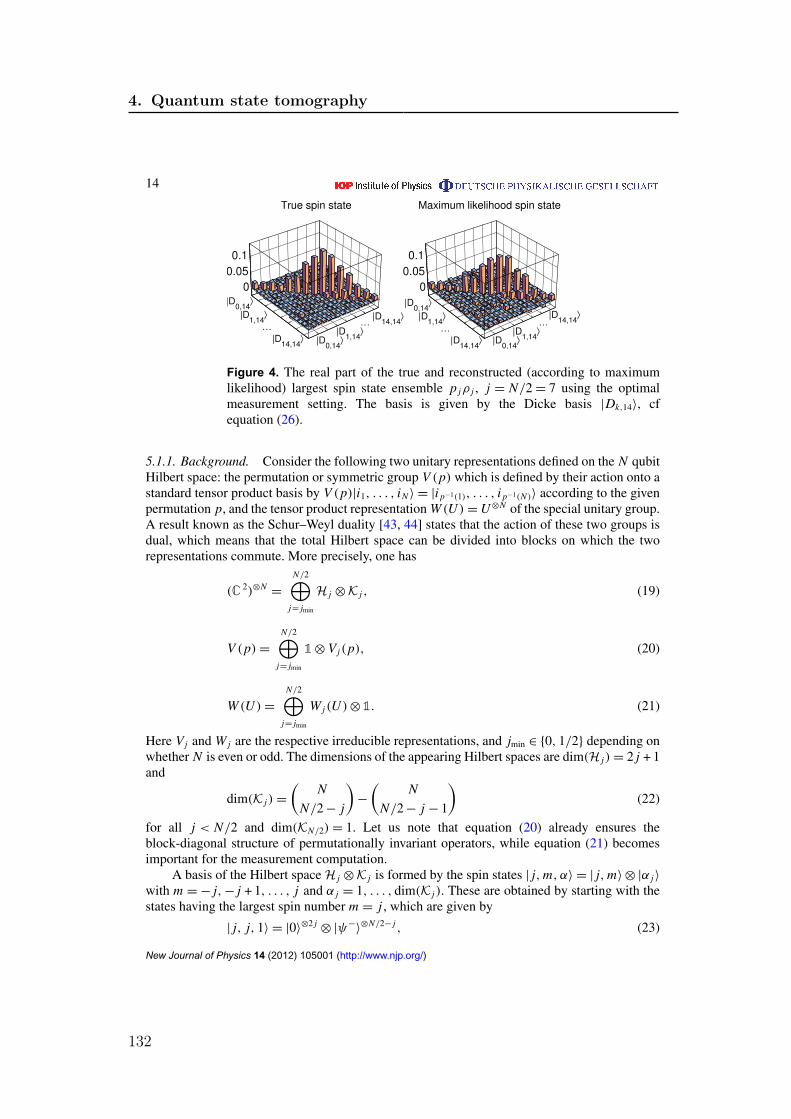
14
Figure 4. The real part of the true and reconstructed (according to maximumlikelihood) largest spin state ensemble p jρ j , j = N/2 = 7 using the optimalmeasurement setting. The basis is given by the Dicke basis |Dk,14〉, cfequation (26).
5.1.1. Background. Consider the following two unitary representations defined on the N qubitHilbert space: the permutation or symmetric group V (p) which is defined by their action onto astandard tensor product basis by V (p)|i1, . . . , iN 〉 = |i p−1(1), . . . , i p−1(N )〉 according to the givenpermutation p, and the tensor product representation W (U )= U⊗N of the special unitary group.A result known as the Schur–Weyl duality [43, 44] states that the action of these two groups isdual, which means that the total Hilbert space can be divided into blocks on which the tworepresentations commute. More precisely, one has
(C2)⊗N=
N/2⊕j= jmin
H j ⊗K j , (19)
V (p)=
N/2⊕j= jmin
1 ⊗ V j(p), (20)
W (U )=
N/2⊕j= jmin
W j(U )⊗ 1. (21)
Here V j and W j are the respective irreducible representations, and jmin ∈ {0, 1/2} depending onwhether N is even or odd. The dimensions of the appearing Hilbert spaces are dim(H j)= 2 j + 1and
dim(K j)=
(N
N/2 − j
)−
(N
N/2 − j − 1
)(22)
for all j < N/2 and dim(KN/2)= 1. Let us note that equation (20) already ensures theblock-diagonal structure of permutationally invariant operators, while equation (21) becomesimportant for the measurement computation.
A basis of the Hilbert spaceH j ⊗K j is formed by the spin states | j,m, α〉 = | j,m〉 ⊗ |α j〉
with m = − j,− j + 1, . . . , j and α j = 1, . . . , dim(K j). These are obtained by starting with thestates having the largest spin number m = j , which are given by
| j, j, 1〉 = |0〉⊗2 j
⊗ |ψ−〉⊗N/2− j , (23)
New Journal of Physics 14 (2012) 105001 (http://www.njp.org/)
4. Quantum state tomography
132

15
| j, j, α〉 =
∑p
c j,pV (p)| j, j, 1〉, (24)
for all α > 2. The coefficients c j,p must ensure that the states | j, j, α〉 are orthogonal; otherwisetheir choice is completely free since the detailed structure of different α’s is not important. Thefull basis is obtained by subsequently applying the ladder operator J− =
∑Nn=1 σ−;n to decrease
the spin number m. Here σ−;n refers to the operator with σ− = (σx − iσy)/2 on the nth qubit andidentity on the rest. Thus in total the basis becomes
| j,m, α〉 =N J j−m− | j, j, α〉, (25)
with appropriate normalizations N . Note that the subspace corresponding to the highest spinnumber j = N/2 is also called the symmetric subspace, which contains many important statessuch as the Greenberger–Horne–Zeilinger or Dicke states, which using the spin states read as
|GHZ〉 =1
√2
(|0〉
⊗N + |1〉⊗N)=
1√
2(|N/2, N/2, 1〉 + |N/2,−N/2, 1〉), (26)
|Dk,N 〉 =N[|1〉
⊗k⊗ |0〉
⊗N−k]
PI= |N/2, N/2 − k, 1〉. (27)
5.1.2. Permutationally invariant states and measurement operators. Let us now employ thisresult in order to derive a generic form for permutationally invariant states; we give the prooffor completeness.
Proposition 5.1 (Permutationally invariant states). Any permutationally invariant state of Nqubits ρPI defined via equation (1) can be written as
ρPI =
N/2⊕j= jmin
p jρ j ⊗1
dim(K j); (28)
hence it is fully characterized by the ensemble p jρ j . Moreover, ρPI is a density operator if andonly if all ρ j are density operators and p j a probability distribution.
Proof. The proposition follows using the representation V (p) given by equation (20) in thedefinition of the states, cf equation (1), and then applying Schur’s lemma [43, 44]. This lemmastates that any linear operator A fromK j toKi which commutes with all elements p of the groupVi(p)A = AV j(p) must either be zero if i and j label different irreducible representations orA = c1 if they are unitarily equivalent. Since API = 1/N !
∑p Vi(p)AV j(p)† fulfils this relation,
one obtains1
N !
∑p
Vi(p)AV j(p)†= δi j tr(A)
1
dim(K j). (29)
The normalization can be checked taking the trace on both sides. Adding appropriate identitiesprovides
1
N !
∑p
1 ⊗ Vi(p)B1 ⊗ V j(p)†= δi j trK j (B)⊗
1
dim(K j), (30)
where B should now be a linear operator from H j ⊗K j to Hi ⊗Ki .
New Journal of Physics 14 (2012) 105001 (http://www.njp.org/)
4.3. Publications
133

16
Finally, let Pj denote the projector onto H j ⊗K j , and using equation (30) yields
ρPI =1
N !
∑p
V (p)ρV (p)† =
∑i,i ′, j, j ′
1
N !
∑p
Pi V (p)Pi ′ρPj V (p)† Pj ′ (31)
=
∑i, j
{1
N !
∑p
Pi [1 ⊗ Vi(p)]PiρPj [1 ⊗ V j(p)]† Pj
}(32)
=
∑i, j
Pi
[δi j trK j (PiρPj)⊗
1
dim(K j)
]Pj (33)
=
⊕j
trK j (PjρPj)⊗1
dim(K j), (34)
which provides the general structure.The state characterization part follows because positivity of a block matrix is equivalent to
positivity of each block. ut
Next let us concentrate on the measurement part. Although the block decompositionfollows already from the previous proposition, it is here more important to obtain an efficientcomputation of each measurement block for the selected setting.
Proposition 5.2 (Measurement operators). The POVM elements Mak as defined in equa-
tion (2) for any local setting a ∈ R3 can be decomposed as Mak =
⊕j Ma
k, j ⊗ 1 with
Mak, j = W j(Ua)M
e3k, j W j(Ua)
†. (35)
The unitary is given by W j(Ua)= exp(−i∑
l tl Sl, j) using the spin operators Sl, j in dimension2 j + 1, while the coefficients tl are determined by Ua = exp(−i
∑l tlσl/2) which satisfies a · Eσ =
UaσzU †a . For the measurement in the standard basis a = e3 one obtains
Me3k, j = | j, N/2 − k〉〈 j, N/2 − k| (36)
if − j 6 N/2 − k 6 j and zero otherwise.
Proof. The basic idea is to consider the measurement in an arbitrary local basis a by a rotationfollowed by the collective measurement in the standard basis. The block decomposition isobtained as follows:
Mak = U⊗N
a Me3k U †⊗N
a = W (Ua)
⊕j
Me3k, j ⊗ 1
W (Ua)† (37)
=
⊕j
W j(Ua)Me3k, j W j(Ua)
†⊗ 1. (38)
The first step holds because Ua satisfies |i〉a〈i | = Ua|i〉〈i |U †a , while the block decomposition of
the standard basis measurement Me3k is employed afterwards. In the last part one uses the tensor
product representation given by equation (21).
New Journal of Physics 14 (2012) 105001 (http://www.njp.org/)
4. Quantum state tomography
134

17
Since one knows that W j is irreducible it can be uniquely written in terms of its Lie algebrarepresentation dW j as W j(Ua)= W j(e−iX)= e−idW j (X), which is given by the spin operators inthis case, i.e. dW j(σl/2)= Sl, j [45].
Thus we are left to compute the measurement blocks Me3k, j for the standard basis. Note
it is sufficient to evaluate Me3k, j ⊗ |1 j〉〈1 j | such that one can employ the spin basis states
| j,m, 1〉 as introduced in section 5.1.1. At first, note that Me3k exactly contains k projections
onto |0〉, while each basis state | j,m, 1〉 possesses (N/2 + m) zeros. Therefore one obtainsMe3
k, j | j,m, 1〉 ∝ δk,N/2+m| j,m, 1〉. Since each POVM has to resolve the identity this is onlypossible if each Me3
k, j is the stated rank-1 projector on the basis states. ut
Finally one still needs to express Ua = exp(−i∑
l tlσl/2) for the chosen setting a ∈ R3.Since this can be related to a familiar rotation [45] these coefficients can be expressed astl = (θ n)l via a rotation about an angle θ around the axis n. Since this rotation should turne3 into a, its parameters are given by
n =e3 × a
‖e3 × a‖2, (39)
θ = arccos(e3 · a), (40)
and n = e1 (or any other orthogonal vector) if a = ±e3.
5.2. Convex optimization
In this part, we collect some more details of the described convex optimization algorithm; forcomplete coverage see the book [36].
Each unconstrained optimization given by equation (14) is solved via a damped Newtonalgorithm. The minimization of f (x)= F[ρ(x)] − t log[det ρ(x)] is obtained by an iterativeprocess. In order to determine a search direction at a given iterate xn, one minimizes thequadratic approximation
f (xn +1x)≈ f (xn)+ ∇ f (xn)T1x + 121x T
∇2 f (xn)1x . (41)
This reduces to solving a linear set of equations called the Newton equation
∇2 f (xn)1xnt = −∇ f (xn), (42)
which determines the search direction 1xnt. The step length s for the next iterate xn+1=
xn + s1xnt is chosen by a backtracking line search. Here one picks the largest s = maxk∈N βk
with β ∈ (0, 1) such that the iterate stays feasible ρ(xn+1) > 0 and that the function valuedecreases sufficiently, i.e. f (xn+1)6 f (xn)+αs∇ f (xn)T1xnt with α ∈ (0, 0.5). The process isstopped if one has reached an appropriate solution, which can be identified by ‖∇ f (xn)‖26 ε.If the initial point xstart is already sufficiently close to the true solution then the whole algorithmconverges quadratically, i.e. the precision gets doubled at each step.
At this point, let us give the gradient and Hessian of the appearing functions. For the barrierterm ψ(x)= − log[det ρ(x)] restricted to the positive domain ρ(x)= 1/ dim(H)+
∑i xi Bi>0,
one obtains [36]
∂ψ(x)
∂xi= − tr[ρ(x)−1 Bi ], (43)
New Journal of Physics 14 (2012) 105001 (http://www.njp.org/)
4.3. Publications
135

18
∂2ψ(x)
∂x j∂xi= tr[ρ(x)−1 B jρ(x)
−1 Bi ]. (44)
Equation (44) shows that the Hessian of the penalty term ∇2ψ(x) > 0 is positive definite,
such that ψ(x) is indeed convex. The derivatives of the preferred fit function can be computeddirectly. For instance, using the likelihood function Fml(x)= −
∑k fk log pk(x) with pk(x)=
tr[ρ(x)Mk], they read
∂Fml(x)
∂xi= −
∑k
fk
pk(x)tr(Bi Mk), (45)
∂2 Fml(x)
∂x j∂xi=
∑k
fk
p2k(x)
tr(B j Mk)tr(Bi Mk). (46)
The bottleneck of such an algorithm is the actual computation of the second derivatives.Although the expansion coefficients of each measurement tr(B j Mk) can be computed inadvance, it is still necessary to compute equation (46) anew at each point x due to thedependence of pk(x). With respect to that, the least squares fit function bears a great advantagesince its Hessian is constant, i.e. ∂ j∂i Fls(x)= 2
∑k wktr(B j Mk)tr(Bi Mk), such that one saves
time on this part.Finally, let us comment on the optimality conditions, known as the Karush–Kuhn–Tucker
conditions [36]. A given x? is the global solution of the convex problem given by equation (13)if and only if14 there exists an additional Lagrange multiplier Z ? (as given in the equationsbeneath) such that the pair (x?,3?) satisfies
∂
∂xiF(x?)− tr[3?Bi ] = 0, ∀i, (47)
3? > 0, ρ(x?)> 0, (48)
tr[3?ρ(x?)] = 0. (49)
Given the solution x tsol of the corresponding unconstrained problem with penalty parameter t ,
it follows from ∇ f (x tsol)= 0 using equation (43) that the gradient conditions are satisfied with
3t = tρ(x tsol)
−1 being the Lagrange multiplier. This pair (x tsol,3t) also satisfies equation (48);
only the duality gap condition tr[3tρ(x tsol)] = t dim(H) > 0 does not hold exactly. However,
this quantity appears in the following inequality:
F(x tsol)− tr[3tρ(x
tsol)] = min
x :ρ(x)>0F(x)− tr[3tρ(x)] (50)
6 minx :ρ(x)>0
F(x)= F(xsol). (51)
Here one used that x tsol is the solution of F(x)− tr[3tρ(x)] because the gradient vanishes
(and the solution is not at the border), and tr[3tρ(x)]> 0 for the inequality. This is the statedaccuracy given by equation (15) which relates the function value of x t
sol to the true solution xsol.
14 Sufficiency holds under the Slater regularity condition that demands a strictly feasible point ρ(x) > 0, whichnaturally holds for state reconstruction problems.
New Journal of Physics 14 (2012) 105001 (http://www.njp.org/)
4. Quantum state tomography
136

19
5.3. Additional tools
5.3.1. Optimization of measurement settings. Measurement settings, each described by a unitvector ai ∈ R3 as explained in section 2.1, are chosen to optimize a figure of merit characterizinghow well a given permutationally invariant target state ρtar can be reconstructed. As such aquality measure we use the sum of errors for the tomographically complete operator set of alltensor products of Pauli operators. Note that a permutationally invariant state ρPI is alreadyuniquely determined by its generalized Bloch vector [17] defined as
bklmn = tr([σ⊗k
x ⊗ σ⊗ly ⊗ σ⊗m
z ⊗ 1⊗n]
PIρPI
)(52)
with natural numbers satisfying k + l + m + n = N . Consequently, the total error of all Blochvector elements is given by
E2total(ai , ρtar)=
∑k,l,m,n
(N
k, l,m, n
)E2
bklmn(ai , ρtar), (53)
where the multinomial coefficient weights the error of each generalized Bloch vector by itsnumber of appearance in a generic Pauli product decomposition.
The error of each Bloch vector element must now be related to the carried outmeasurements. For that, note that each Bloch vector element can be expressed as
bklmn =
∑i
cklmni tr([(ai · Eσ)⊗N−n
⊗ 1⊗n]PIρtar) (54)
using appropriate coefficients cklmni and the expectation values of [(ai · Eσ)⊗N−n
⊗ 1⊗n]PI whichcan be computed from the coarse-grained measurement outcomes Mai
k of setting ai as given byequation (2) using linear combinations. Assuming independent errors, one obtains
E2bklmn
(ai , ρtar)=
∑i
cklmni E2
ρtar
([(ai · Eσ)⊗N−n
⊗ 1⊗n]PI
). (55)
The detailed form of the error expression E2ρtar([(ai · Eσ)⊗N−n
⊗ 1⊗n]PI) may depend on the actualphysical realization, but we assume the following form:
E2ρtar
([(ai · Eσ)⊗N−n
⊗ 1⊗n]PI
)= K1ρtar
([(ai · Eσ)⊗N−n
⊗ 1⊗n]PI
), (56)
where1ρ[A] = tr(ρA2)− [tr(ρA)]2 is the standard variance and K is a state-independent factor.This form fits well, for example, to the common error model in photonic experiments wherecount rates are assumed to follow a Poissonian distribution. For more details of this derivation,see [17].
For large qubit numbers, N , this optimization is carried out iteratively. Starting fromrandomly chosen measurement directions or from vectors which are uniformly distributedaccording to some frame potential [46], one searches for updates according to
a′
i =pan
i + (1 − p)ri
‖pani + (1 − p)ri‖
. (57)
Here ani is the current iterate, p < 1 a probability close to 1 and ri are randomly chosen unit
vectors. If this new set of directions a′
i leads to a smaller total error E2total(a
′
i , ρtar) than theprevious set, then these new measurement settings form the next iterate an+1
i = ani ; otherwise
this procedure is carried out once more. This process is repeated until the total error does notdecrease anymore. This way of optimizing the measurements requires a method for computing
New Journal of Physics 14 (2012) 105001 (http://www.njp.org/)
4.3. Publications
137

20
the total error E2total(ai , ρtar) for a given set of measurements ai . Using the generalized Bloch
vector or the spin ensemble this computation can be carried out again efficiently for larger qubitnumbers N .
Although this algorithm is not proven to attain the true global optimum it is still astraightforward technique to obtain good settings. In the end this is often sufficient, recallingthat the true unknown state can deviate from the target state and that one considers ‘just’ anoverall single figure of merit. For our simulations we always use the optimized settings for thetotally mixed state; a reasonable guess if no extra information is available [47].
Regarding this point, we finally like to add that if one does not employ the minimal numberof measurement settings, but rather an over-complete set, e.g. four times as many settings butfour times fewer measurements per setting, then the procedure is quite insensitive to the chosenmeasurement directions. Hence, in many practical situations the search for optimal directionsmight not even be necessary and randomly chosen measurement directions suffice equally well.
5.3.2. Statistical pretest. Via the pretest one estimates the fidelity between the true ρtrue
and the best permutationally invariant state FPI(ρtrue)= maxρPI>0 tr(√√
ρtrueρPI√ρtrue) using
only measurement results from a few settings a ∈ T , e.g. employing only T = {e1, e2, e3}.Depending on this quantity, one decides on whether permutationally invariant tomography isworth continuing. As explained in detail in [17], this fidelity can be bounded by
FPI(ρtrue)> [tr(ρtrue Z)]2 (58)
with an operator Z =∑
zak Ma
k being built up by the carried out measurements Mak given by
equation (2) and satisfying Z 6 Psym, where Psym denotes the projector onto the symmetricsubspace.
The expansion coefficients zak should be optimized to attain the best lower bound. For a
given target state ρtar this problem can be cast into a semidefinite program [36, 48] that canbe solved efficiently using standard numerical routines. However, for larger qubit numbers onemust again employ the block structure of the measurement operators as given by equation (9) tohandle the operator inequality. Note that the projector on the symmetric subspace has a Blockstructure Psym, j = δ j,N/21. Then the final problem reads as
maxz
∑a∈T,k
zak tr(ρtar M
ak )
(59)
s.t.∑
a∈T,k
zak Ma
k, j=N/2 6 1,∑
a∈T,k
zak Ma
k, j 6 0, ∀ j < N/2.
If one experimentally implements this pretest, one must account for additional statisticalfluctuations. For the chosen Z , one can employ the sample mean Z =
∑za
k f ak using the
observed frequencies f ak = na
k/NR in NR repetitions of setting a, as an estimate of the trueexpectation value tr(ρtrue Z). This sample mean Z will fluctuate around the true mean butlarge deviations will become less likely, such that for an appropriately chosen ε the quantitysign(Z − ε)(Z − ε)2 is a lower bound to the true fidelity at the desired confidence level. Theproof essentially uses the techniques employed in [49, 50].
Proposition 5.3 (Statistical pretest). For any Z =∑
zak Ma
k 6 Psym let Z =∑
zak na
k/NR
denote the sample mean using NR repetitions for setting a ∈ T . If the data are generated by
New Journal of Physics 14 (2012) 105001 (http://www.njp.org/)
4. Quantum state tomography
138

21
the state ρtrue, then
Prob[FPI(ρtrue)> sign(Z − ε)(Z − ε)2
]> 1 − exp(−2NRε
2/C2z ) (60)
with C2z =
∑a
(zs
max − zsmin
)2where za
max/min are the respective optima for setting a over alloutcomes k.
Proof. The given statement follows along
Prob[FPI(ρtrue)> sign(Z − ε)(Z − ε)2
]> Prob
[tr(ρtrue Z)> Z − ε
], (61)
> 1 − Prob[tr(ρtrue Z)6 Z − ε
]> 1 − exp(−2NRε
2/C2z ). (62)
Here the first inequality holds because the set of outcomes satisfying {nak : tr(ρtrue Z)> Z − ε}
is a subset of {nak : FPI(ρtrue)> sign(Z − ε)(Z − ε)2} using equation (58). In the last inequality
we use the Hoeffdings tail inequality [51] to bound Prob[tr(ρtrue Z)6 Z − ε]. ut
Note that this pretest can also be applied after the whole tomography scheme in whichcase the projector Psym =
∑za
k Mak becomes accessible. Moreover, let us point out that a strong
statistical significance, or a low ε respectively, might not be achieved with the best expectationvalue as given by equation (59) [52]; hence, optimizing Z for a rather mixed state is often better.
Finally, let us remark that the pretest can be improved by additional projectors, see thesupplementary material of [17]. This leads to the bound FPI(ρtrue)>
∑j p2
j with p j being theweight of the corresponding spin- j state of the permutationally invariant part of ρtrue as givenin equation (7). From this expression one sees that this test only works well for states having arather large weight on one of these spin states. Others, like the totally mixed state, while clearlybeing permutationally invariant, are not identified as states close to the permutationally invariantsubspace. This is in stark contrast to compressed sensing where the certificate succeeds for thewhole class of low-rank target states [10].
5.3.3. Entanglement and the MaxLik–MaxEnt principle. Following the last comment fromthe previous subsection, we want to argue that even in the case of an inefficient certificate,permutationally invariant state reconstruction as given by equation (5) is meaningful. Firstlywe would like to emphasize that the permutationally invariant part of any density operatorcorresponds to a good representative to investigate the entanglement properties of the true,unknown state. This is because the transformation given by equation (1) can be achieved bypermutations or multiple swap operations together with classical mixing, whereby entanglementcannot be created [53]. Thus if the permutationally invariant part of the density operator isentangled this holds true also for the real state. In addition, any symmetric entanglementmeasure, i.e. all commonly known ones, can only decrease under this operation, thereby evenquantification is faithful [54].
Secondly, permutationally invariant state reconstruction also represents the solution of themaximum-likelihood maximum-entropy principle as introduced in [55], which goes as follows:if the carried out measurements are not tomographically complete, then there is, in general, nota single state ρml that maximizes the likelihood but rather a complete set of them. In order tosingle out a ‘good’ representative, the authors of [55] propose to choose the state that has thelargest entropy, which, according to the Jaynes principle [47], is the special state for which onehas the fewest information.
New Journal of Physics 14 (2012) 105001 (http://www.njp.org/)
4.3. Publications
139

22
Proposition 5.4 (Permutationally invariant MaxLik–MaxEnt principle). Using the de-scribed permutationally invariant tomography scheme, the reconstructed permutationallyinvariant state given by equation (5) (with the likelihood function) is also the solution of themaximum-likelihood maximum-entropy principle.
Proof. Since the measurements given by equation (2) are invariant and tomographicallycomplete for permutationally invariant states, all density operators with the same spin ensembleas ρPI have the same maximum likelihood. According to Ref. [47], the state with maximalentropy and consistent with a given set of expectation values for operators Ma
k has the formρ ∝ exp(
∑a,k λ
ak Ma
k ). The Lagrange multipliers λak ∈ R must be chosen such that the given
expectation values match. However, because all Mak are permutationally invariant we can
employ the block decomposition given by equation (9) and finally obtain exp(∑
a,k λak Ma
k )=
exp(⊕ j∑
a,k λak Ma
k, j ⊗ 1)= ⊕ j exp(∑a
k λak Ma
k, j)⊗ 1. Hence we obtain the same structure asρPI, which therefore is also the state with maximum entropy. ut
6. Conclusion and outline
In this paper, we have provided all the necessary ingredients to carry out permutationallyinvariant tomography [17] in experiments with large qubit numbers. This includes, besidesscheme-specific tasks such as the statistical pretest and the optimization of the measurementsettings, in particular the state reconstruction part. Accounting for statistical fluctuations dueto a finite number of data, this reconstruction demands the solution of a nonlinear large-scale optimization problem. We achieve this, firstly, by using a convenient toolbox to store,characterize and process permutationally invariant states, which largely reduces the dimensionof the underlying problem and, secondly, by using convex optimization, which is superiorcompared to commonly used numerical routines in many respects. This makes permutationallyinvariant tomography a complete tomography method requiring only moderate measurementand data analysis effort.
There are many questions one may pursue in this direction: firstly, let us stress thatthe current prototype implementation is still not optimal. As explained, the bottleneck isthe computation of the second derivatives; hence, we strongly believe that Hessian freeoptimization, like quasi-Newton or conjugate gradients [56], or the use of other barrier functionsmore tailored to linear matrix inequalities [57] are likely to push the reconstruction limitfurther. Secondly, it is natural to try to exploit other symmetries in the development of‘symmetry’ tomography protocols; that is, tomography should work for all states that remaininvariant under the action of a specific group. Clearly, any symmetry decreases the numberof state-dependent parameters, but the challenge is to devise efficient local measurementstrategies. Interesting classes here are graph-diagonal [58] or, more general, locally maximallyentangleable states [59], translation or shift-invariant states [60], or U⊗N invariant states[61, 62]. Thirdly, it is worth investigating to what extent particularly designed state tomographyprotocols are useful for further tasks, such as process tomography for quantum gates. Forinstance, permutationally invariant tomography might be unable to resolve the Toffoli gate [63]directly, but since the operation on all N target qubits is symmetric, a permutationally invariantresolution of this subspace (and the additional control qubit) might be sufficient. Finally, let uspoint out that permutationally invariant tomography can be further restricted to the symmetric
New Journal of Physics 14 (2012) 105001 (http://www.njp.org/)
4. Quantum state tomography
140

23
subspace, which often contains the desired states. This is reasonable since we have seen that thepretest is only good if the unknown state has a large weight in one of the spin states. However,since the symmetric subspace grows only linearly with the number of particles, this tomographyscheme can analyse many more qubits efficiently.
Acknowledgments
We thank M Kleinmann, B Kraus, T Monz, L Novo, P Schindler and J Wehr for stimulatingdiscussions on the topic and technicalities. This work was supported by the FWF (STARTprize Y376-N16), the EU (Project Q-ESSENCE and Marie Curie CIG 293993/ENFOQI), theBMBF (Chist-Era Project QUASAR), the ERC (Starting Grant GEDENTQOPT), the QCCCof the Elite Network of Bavaria, the Spanish MICINN (project no. FIS2009-12773-C02-02),the Basque Government (project no. IT4720-10) and the National Research Fund of HungaryOTKA (contract no. K83858).
References
[1] Paris M G A and Rehacek J (ed) 2004 Quantum State Estimation (Berlin: Springer)[2] Haffner H et al 2005 Nature 438 643[3] Kiesel N, Schmid C, Toth G, Solano E and Weinfurter H 2007 Phys. Rev. Lett. 98 063604[4] James D F V, Kwiat P G, Munro W J and White A G 2001 Phys. Rev. A 64 052312[5] Renes J M, Blume-Kohout R, Scott A J and Caves C M 2004 J. Math. Phys. 45 2171[6] Monz T, Schindler P, Barreiro J T, Chwalla M, Nigg D, Coish W A, Harlander M, Haensel W, Hennrich M
and Blatt R 2011 Phys. Rev. Lett. 106 130506[7] Yao X C, Wang T X, Xu P, Lu H, Pan G S, Bao X H, Peng C Z, Lu C Y, Chen Y A and Pan J W 2012 Nature
Photon. 6 225[8] Huang Y F, Liu B H, Peng L, Li Y H, Li L, Li C F and Guo G C 2011 Nature Commun. 2 546[9] Gross D, Liu Y K, Flammia S T, Becker S and Eisert J 2010 Phys. Rev. Lett. 105 150401
[10] Gross D 2011 IEEE Trans. Inf. Theory 57 1548[11] Flammia S T, Gross D, Liu Y K and Eisert J 2012 Quantum tomography via compressed sensing: error
bounds, sample complexity and efficient estimators arXiv:1205.2300[12] Cramer M, Plenio M B, Flammia S T, Gross D, Bartlett S D, Somma R, Landon-Cardinal O, Liu Y K and
Poulin D 2010 Nature Commun. 1 9[13] Baumgratz T, Gross D, Cramer M and Plenio M B 2012 Scalable reconstruction of density matrices
arXiv:1207.0358[14] Landon-Cardinal O and Poulin D 2012 Practical learning method for multi-scale entangled states
arXiv:1204.0792[15] Yin J O S and van Enk S J 2011 Phys. Rev. A 83 062110[16] Guta M, Kypraios T and Dryden I 2012 Rank-based model selection for multiple ions quantum tomography
arXiv:1206.4032[17] Toth G, Wieczorek W, Gross D, Krischek R, Schwemmer C and Weinfurter H 2010 Phys. Rev. Lett.
105 250403[18] Moroder T, Kleinmann M, Schindler P, Monz T, Guhne O and Blatt R 2012 Detection of systematic errors in
quantum experiments arXiv:1204.3644[19] D’Ariano G M, Maccone L and Paini M 2003 J. Opt. B: Quantum Semiclass. Opt. 5 77[20] Karassiov V P 2005 J. Russ. Laser Res. 26 484[21] Adamson R B A, Shalm L K, Mitchell M W and Steinberg A M 2007 Phys. Rev. Lett. 98 043601
New Journal of Physics 14 (2012) 105001 (http://www.njp.org/)
4.3. Publications
141
24
[22] Adamson R B A, Turner P S, Mitchell M W and Steinberg A M 2008 Phys. Rev. A 78 033832[23] Hradil Z 1997 Phys. Rev. A 55 R1561[24] Langford N K 2007 Encoding, manipulating and measuring quantum information in optics PhD Thesis School
of Physical Sciences, University of Queensland[25] Blume-Kohout R 2010 Phys. Rev. Lett. 105 200504[26] Efron B and Tibshirani R J 1994 An Introduction to the Bootstrap (London: Chapman and Hall)[27] Christandl M and Renner R 2011 Reliable quantum state tomography arXiv:1108.5329[28] Blume-Kohout R 2012 Robust error bars for quantum tomography arXiv:1202.5270[29] Mood A F 1974 Introduction to the Theory of Statistics (New York: McGraw-Hill)[30] Cirac J I, Ekert A K and Macchiavello C 1999 Phys. Rev. Lett. 82 4344[31] Demkowicz-Dobrzanski R 2005 Phys. Rev. A 71 062321[32] Chase B A and Geremia J M 2008 Phys. Rev. A 78 052101[33] Baragiola B Q, Chase B A and Geremia J M 2010 Phys. Rev. A 81 032104[34] Hradil Z, Rehacek J, Fiurasek J and Jezek M 2004 Lect. Notes Phys. 649 59[35] Reimpell M 2008 Quantum information and convex optimization PhD Thesis Technische Universitat
Braunschweig[36] Boyd S and Vandenberghe S 2004 Convex Optimization (Cambridge: Cambridge University Press)[37] Kosut R L, Walmsley I A and Rabitz H 2004 Optimal experiment design for quantum state and process
tomography and Hamiltonian parameter estimation arXiv:quant-ph/0411093[38] Glancy S, Knill E and Girard M 2012 Gradient-based stopping rules for maximum-likelihood quantum-state
tomography arXiv:1205.4043[39] Rehacek J, Hradil Z and Jezek M 2001 Phys. Rev. A 63 040303[40] Rehacek J, Hradil Z, Knill E and Lvovsky A I 2007 Phys. Rev. A 75 042108[41] Nielsen M A and Chuang I L 2000 Quantum Computation and Quantum Information (Cambridge: Cambridge
University Press)[42] Zyczkowski K and Sommers H J 2001 J. Phys. A: Math. Gen. 34 7111[43] Simon B 1996 Representations of Finite and Compact Groups (Graduate Studies in Mathematics vol 10)
(Providence, RI: American Mathematical Society)[44] Christandl M 2006 The structure of bipartite quantum states—insights from group theory and cryptography
arXiv:0604183[45] Hall B C 2003 Lie Groups, Lie Algebras and Representations: An Elementary Introduction (New York:
Springer)[46] Gross D, Audenaert K and Eisert J 2007 J. Math. Phys. 48 052104[47] Jaynes E 1957 Phys. Rev. 108 171[48] Toth G, Wieczorek W, Krischek R, Kiesel N, Michelberger P and Weinfurter H 2009 New J. Phys. 11 083002[49] Flammia S T and Liu Y K 2011 Phys. Rev. Lett. 106 230501[50] da Silva M P, Landon-Cardinal O and Poulin D 2011 Phys. Rev. Lett. 107 210404[51] Hoeffding W 1963 J. Am. Stat. Assoc. 58 301[52] Jungnitsch B, Niekamp S, Kleinmann M, Guhne O, Lu H, Gao W B, Chen Y A, Chen Z B and Pan J W 2010
Phys. Rev. Lett. 104 210401[53] Busch P 2003 Int. J. Theor. Phys. 42 937[54] Horodecki K, Horodecki M and Horodecki P 2010 Quantum Inform. Comput. 10 0901[55] Teo Y S, Zhu H B-G, Englert B G, Rehacek J and Hradil Z 2011 Knowledge and ignorance in incomplete
quantum state tomography arXiv:1102.2662[56] Geiger C and Kanzow C 1999 Numerische Verfahren zur Losung unrestringierter Optimierungsaufgaben
(Berlin: Springer)[57] Kocvara M and Stingl M 2003 Optim. Methods Softw. 18 317[58] Hein M, Dur W, Eisert J, Raussendorf R, Van den Nest M and Briegel H J 2005 Proc. Int. School of Physics
‘Enrico Fermi’ on ‘Quantum Computers, Algorithms and Chaos’, Varenna, Italy
New Journal of Physics 14 (2012) 105001 (http://www.njp.org/)
4. Quantum state tomography
142

25
[59] Kruszynska C and Kraus B 2009 Phys. Rev. A 79 052304[60] O’Connor K M and Wootters W K 2001 Phys. Rev. A 63 052302[61] Eggeling T and Werner R F 2001 Phys. Rev. A 63 042111[62] Cabello A 2003 J. Mod. Opt. 50 10049[63] Monz T, Kim K, Hansel W, Riebe M, Villar A S, Schindler P, Chwalla M, Hennrich M and Blatt R 2009 Phys.
Rev. Lett. 102 040501
New Journal of Physics 14 (2012) 105001 (http://www.njp.org/)
4.3. Publications
143

4. Quantum state tomography
144

5. Systematic errors of standardquantum state estimation
Applying the tomography schemes described in section 4.1.1 and 4.1.2 often resultsin a density matrix which fails to be physical, i.e., some of its eigenvalues arenegative. Since the eigenvalues are associated with probabilities, and are thusconstrained to lie within the interval [0, 1], this poses a serious conceptual problem.One might argue that as long as a value of 0 lies within the error, there is noreason to bother. Nevertheless, the question arises how to deduce entanglementmeasures or mixed state fidelities for such states, as they might be mathematicallyill-defined or just meaningless.
Typically, in such a situation, maximum likelihood or least squares fitting algo-rithms as discussed in section 4.1.3 are applied which guarantee to deliver a phys-ical result. Recently, various alternative approaches have been proposed which allrestrict the result to lie within the physical regime [281, 282] and even, althoughnumerically expensive, allow to calculate meaningful confidence and credibilityregions for the estimate itself [263, 283–287]. Furthermore, quantum state tomog-raphy and the closely related quantum process tomography could even be adoptedto detect systematic errors in the alignment of an experiment [246, 288–292].
In this chapter, several reasons for seemingly unphysical results in tomographyexperiments will be discussed. In section 5.1, it will be shown that the origin ofsuch unphysical results can be manifold, ranging from experimental imperfectionsto the orientation of the state with respect to the measurement axis. Then, insection 5.2, it will be shown that implying additional constraints in quantum stateestimation, such as non-negativity of a quantum state, can introduce systematicerrors. In estimation theory, such errors are well-known under the term bias [80,293] (see publication P5.1). The size of these errors for derived quantities like,e.g., the fidelity with respect to a target state is investigated on the example ofa four-qubit GHZ state mixed with white noise. Furthermore, it will be proventhat an estimator which always delivers a state obeying the physicality constraintcannot be unbiased. In publication P5.1, the way towards an, at least partial,solution of this problem is presented. There, it is shown that any quantity thatis given by a convex function, like, e.g., many entanglement measures, can beapproximated by a linear function for which meaningful bounds together withsimple to calculate errors can be given. However, as these bounds are derivedwith the aid of Hoeffding’s tail inequality [294], they are relatively week.
145

5. Systematic errors of standard quantum state estimation
5.1. Origin of unphysical density matrices
It is known that misalignment in an experimental apparatus can cause inconsis-tencies in the data evaluation process when it remains undetected [288]. Here, bymeans of two illustrative examples, it will be shown that there are several reasonswhy the states as obtained from a tomographic analysis together with linear in-version (see section 4.1) can lead to seemingly unphysical results, i.e., states withat least one negative eigenvalue. More precisely, the misalignment of the exper-imental apparatus is just one possible reason for such unphysical results and, inview of the quality of today’s experiments, it is by far not the most relevant one.Below, a few examples are given, where it is the statistical noise which suffices tocause unphysical estimates.
As a first example, let us consider Pauli tomography of a pure single-qubit state|z+〉 and measurements in the standard bases σx, σy, and σz. When performingmeasurements in the σz basis, the result is always +1 and thus Tz = 1, indepen-dently of the measurement statistics! Consequently, the remaining correlations Tx
XsZ\
XsX
\
+1
0
-1
+10-1
ρ ³ 0
êZ+\
Figure 5.1.: Experimental Pauli tomography of the single-qubit state |z+〉. Forsimplicity, only the x-z plane is shown. The square represents all results that can,at least in principle, be observed in a experiment. All points inside the gray circlerepresent valid quantum states %, i.e, Tr(%) = 1 and % ≥ 0, with the pure stateslying on the rim of the circle. The states represented by the white corners ofthe square correspond to states where the physicality condition % ≥ 0 is violated.Measuring in the σz basis delivers a correlation value of Tz = 1 independentlyof the number of repetitions of the experiment. Then, when measuring in theσx basis afterwards, all resultant states except the one for Tx = 0 lie outsidethe physical regime as indicated by the red line in the figure. However, whenthe number of measurements in the σx basis is odd, Tx 6= 0. Please note thatthis peculiar behavior cannot be overcome by simply improving the measurementstatistics!
146

5.1. Origin of unphysical density matrices
and Ty both have to be 0 because otherwise the state would lie outside the Blochsphere. This can easily be seen by expressing the purity of a single-qubit state interms of its Bloch vector elements, Tr(%2) = 1
2(1+T 2
x +T 2y +T 2
z ) and the fact thatthe purity is bounded from above by 1. Now, when measuring in the σx basis,the correlation Tx can only vanish if the results +1 and −1 are observed with thesame frequency. However, this is not possible if the number of measurements inthe σx basis is odd! For more details, see Fig. 5.1.
The second example to be considered is Pauli tomography of the one parameterfamily of four-qubit states p1⊗4
16+ (1− p)|GHZ4〉〈GHZ4| with p ∈ [0, 1]. The two
extremal cases p = 0 and p = 1 correspond to a GHZ state and to white noise,respectively. Since all the eigenvalues of white noise are 1
2N, i.e., it is a full rank
state, at first glance, one would expect, that it is fairly unlikely to observe negativeeigenvalues in a tomographic experiment. This view is further supported by thefact that the overlap between white noise and any pure state |φ〉 is 〈φ|1⊗N
2N|φ〉 = 1
2N
which means that, in some sense, white noise can be considered to lie in the mid-dle of the state space. However, as can be seen in Fig. 5.2, the opposite turns outto be the case, namely, that on the order of 1000 counts per basis setting (a mea-surement statistics hardly found in multiqubit experiments) are necessary untilone can expect to observe no negative eigenvalues. This counterintuitive behaviorcan be explained by the fact that determining the eigenvalues of a state comeswith some statistical error and that the observed eigenvalues scatter around theirtrue value. Obviously, the smaller the sample size, the larger the scattering isexpected to be. Hence, for small sample sizes, an eigenvalue < 0 lies within thescatter of the respective eigenvalue. Thus, it is likely that at least one of the 2N
eigenvalues is negative and it is therefore normal to observe negative eigenvalueseven for white noise.
As explained in section 4.1.3, when determining % by means of linear inver-sion, one interprets the experimental data from a frequentistic point of view. Theobserved relative frequencies are treated as an approximation to the unknown un-derlying probabilities. In the asymptotic limit, i.e., for infinitely many repetitionsof the experiment, the relative frequencies converge towards the probabilities.Therefore, one might expect that the probability to observe a state with at leastone negative eigenvalue decreases for better and better statistics. In principle, thisview is correct, as can be seen in Fig. 5.2, for values of p > 0. However, for purestates (i.e. p = 0) increasing the sample size does not reduce the number of stateswith at least one negative eigenvalue, as can be seen in Fig. 5.2. This peculiarbehavior comes from the fact that for pure N -qubit states 2N − 1 eigenvalues areexactly 0 and thus every infinitesimal perturbation, as induced for example bystatistical noise, will generally lead to at least one negative eigenvalue .
To show that the above described characteristics of the Pauli tomographyscheme together with linear inversion are no artifact of the considered familyof states, the simulation was repeated for a second family of states, p1⊗4
16+ (1 −
147

5. Systematic errors of standard quantum state estimation
Figure 5.2.: Simulation of Pauli tomography for two one parameter familiesa) p1⊗4
16+ (1 − p)|GHZ4〉〈GHZ4| and b) p1⊗4
16+ (1 − p)|D(2)
4 〉〈D(2)4 | for different
measurement statistics under the assumption of a multinomial distribution ofthe counts. As can be seen in both cases, the percentage of states violating thephysicality condition % ≥ 0, is significant for small sample sizes and high purities.
p)|D(2)4 〉〈D
(2)4 |. Moreover, it has to be excluded that the orientation of the state
with respect to the measurement axes plays a role. Therefore, the Dicke stateD
(2)4 was not expressed in the computational basis (|z+〉 and |z−〉) but rotated
such that |z+〉 −→ |x+〉+ |y+〉+ |z+〉 and |z−〉 −→ |x−〉+ |y−〉+ |z−〉. The resultof the simulation can be seen in Fig. 5.2b). As the similarity between Fig. 5.2a)and Fig. 5.2b) is remarkable, it is save to say that the observed characteristicscan really be attributed to the Pauli tomography scheme together with linearinversion.
Furthermore, in Fig. 5.2, it can be seen that there is a sharp border betweenthe regime where the reconstructed state is almost certainly positive-semidefiniteand where it normally fails to be positive-semidefinite. More precisely, this meansthat when the number of counts surpasses a certain limit, the reconstructed stateis almost for sure physical. By means of random matrix theory, it can be shownthat the eigenvalues of the reconstructed density matrix follow a Wigner semicircledistribution. Additionally, random matrix theory even allows to determine thenumber of counts where the transition between the physical and the unphysicalregime occurs. A detailed discussion of these findings will be given in a futurepublication by Lukas Knips.
148

5.2. Constrained state estimation
5.2. Constrained state estimation
5.2.1. Flaws of constrained state estimation
In order to ensure physicality of an experimentally determined density matrix,the fitting algorithms described in section 4.1.3 are commonly applied. However,at this point, one might ask if this approach really solves the problem of nega-tive eigenvalues or whether it suffers from other shortcomings? To answer thisquestion, a simple numerical experiment shall be performed. In detail, the Paulitomography scheme is simulated on the example of a test state together withdifferent algorithms for data post processing, namely, maximum likelihood, leastsquares, and, for comparison, linear inversion. As a test state, let us consider afour-qubit GHZ state that is mixed with white noise
%GHZ(p) = (1− p) |GHZ4 〉〈GHZ4 | +p1⊗4
16(5.1)
where the parameter p is chosen such that the fidelity with the ideal GHZ stateis 0.8. The reason to consider a mixed state is to avoid possible boundary effectsfrom the border of the state space. The numerical experiment consists of 4 steps:
i) Calculate the expectation values pi for all measurement operators Mi.
ii) Toss coins to generate frequencies fi according to a multinomial distributionwith N counts for every measurement basis.
iii) Reconstruct the state with either procedure for data post processing men-tioned above and, from the result, calculate any quantity of interest.
iv) Repeat steps i)-iv) 500 times
In Fig. 5.3, the result of this numerical experiment for N = 100 with the fidelityas quantity of interest is shown. Ideally, on average, one would expect that allthree methods return a value of 0.8 for the fidelity. However, as can be clearlyseen, both maximum likelihood and, even worse, least squares fitting lead to asystematic underestimation of the fidelity. In detail, maximum likelihood deliversa value of 0.788 ± 0.010 for the fidelity and least squares fitting delivers 0.749 ±0.010. Even if one takes the widths of the distributions into consideration, thevalues are off by one and five standard deviations, respectively. In contrast, thefidelity value of 0.799 ± 0.012 delivered by linear inversion is in agreement withthe true value of 0.8. From an engineering point of view, one might argue thatunderestimating the fidelity is more an inconvenience than an actual problem.However, much worse, other quantities that are used to detected entanglement,like the negativity, are overestimated, see Fig. 5.4 which, as a consequence, canlead to false entanglement detection! In general, this systematic offset depends
149

5. Systematic errors of standard quantum state estimation
10
20
30
40
50
# S
tate
s
60
00.72 0.74 0.76 0.78 0.80 0.82 0.84
Fidelity w.r.t. GHZ4
LINML
LS
Figure 5.3.: Histogram of the fidelity as obtained from 500 independent simu-lations of the Pauli tomography scheme together with three different schemes fordata post processing. The average values delivered by maximum likelihood (ML)and least squares (LS) clearly fluctuate around a value well below the true fidelityof 0.8. This systematic error called bias is not observed for linear inversion (LIN).
on various parameters like, e.g., the system size, the quantity of interest or thestate itself (for details see publication P5.1). Therefore, a later manual correctionof the offset seems unjustifiable!
In mathematical statistics and in the theory of point estimates, such systemat-ical offsets are well-known under the term bias [295]. Adopted to quantum statetomography, an estimator % is called unbiased if it fulfills the relation
E%0(%) ≡∑f
P%0(f)%(f) = %0. (5.2)
Otherwise it is called biased. In order to obtain a more intuitive understandingof the origin of the bias in quantum state estimation consider Fig. 5.5. In sub-figure a), possible results of tomography of a pure state before fitting are shown.Due to statistical noise, many of these results lie outside the physical regime.However, the center of mass of the whole distribution coincides with the true(unknown) state. Subfigure b) shows how maximum likelihood or least squaresfitting change the distribution. All states that were positive-semidefinite remainunchanged whereas all states that were outside the physical regime are mappedon the border of the state space. Consequently, the center of mass of the wholedistribution changes which, as a result, leads to biased state estimation. Pleasenote that linear inversion does not suffer from this problem, i.e., it is unbiasedbecause, according to Eq. 4.12, %lin is a linear function of the frequencies fi and forall frequencies E(fi) = pi holds. In estimation theory it is common knowledge thatapplying additional constraints can lead to biased estimation. In section 5.2.2, itis proven that by adding the physicality constraint any quantum state estimationscheme necessarily becomes biased.
150

5.2. Constrained state estimation
Bipartite Negativity
0.450.35 0.400.300.25
LBLML
LS
20
40
# S
tate
s
60
80
0
separable State + white NoiseGHZ4 State + white Noise
0.05 0.10-0.05 0-0.100.20
100
120
Figure 5.4.: Both maximum likelihood (ML) and least squares (LS) estimationcan lead to a systematic overestimation of the negativity which, in consequence,may lead to false entanglement detection when analyzing separable states as shownin b). As discussed in publication P5.1, linearization of the negativity allows todeduce a lower bound (LBL) such that a valid estimate is obtained.
Figure 5.5.: Enforcing physicality in a quantum state estimation scheme leadsto biased state estimation. Before fitting, the determined states scatter aroundthe true state % with many of them lying outside the physical regime. Fittingalgorithms based on maximum likelihood or a least squares minimization mapall states with negative eigenvalues on the border of the state space. Effectively,this leads to a shift of the center of mass of the distribution of states which issubsequently observed as a bias.
151

5. Systematic errors of standard quantum state estimation
5.2.2. Biasedness and physicality
As shown in section 5.2.1, for sample sizes typical for multiqubit experiments,both maximum likelihood and least squares fitting algorithms lead to systematicdeviations for deduced quantities like, e.g., the fidelity with respect to a targetstate. Thus, the question arises if such deviations are only a shortcoming ofthe respective fitting algorithm and one only needs to find a better algorithmor whether the observed effects are of a more general nature. In the following,it will be proven that as soon as the constraint of non-negativity is imposed,systematic deviations are unavoidable. More precisely, the constraint of non-negativity automatically leads to biased state estimation. The proof given belowis a more detailed version of the proof presented in publication P5.1.
Figure 5.6.: a) A pure quantum state %1 =| ψ1 〉〈ψ1 | is analyzed by meansof quantum state tomography. Because the experimental measurement time isfinite, also the set of acquired experimental data has to be finite. Therefore, onlya subset of states is accessible, here, marked by crosses. b) Enforcing physicalityand unbiasedness of a reconstruction scheme for %1, leads to mapping all possibleresults for tomography of %1 back to %1. c) Now a second pure quantum state%2 =|ψ2 〉〈ψ2 | is to be analyzed which is non-orthogonal to %1 and, therefore, thereare some results which can be obtained for both states. If now the reconstructionscheme shall also be unbiased for %2, all possible results would have to be mappedback to %2. However, this is not possible because some of the results are alreadymapped to %1, here marked in red. Therefore, a reconstruction scheme whichalways returns a valid density operator cannot be unbiased.
Theorem. A reconstruction scheme for quantum state tomography that alwaysyields a valid, i.e., non-negative, density operators is biased.
Proof. Let us consider experimental quantum state tomography with, due tolimited measurement time, a finite sample size. For finite sample sizes, the set offrequencies that can be observed is restricted because all frequencies have to be
152

5.3. Publications
multiples of 1/N where N is a normalization constant that depends on the samplesize (for Pauli tomography N is the number of counts per measurement setting).In Fig. 5.6a), the possible states that can be obtained in a tomography experimentby linear inversion for a certain measurement statistic are marked by crosses. Nowconsider tomography of a pure pure quantum state %1 =| ψ1 〉〈ψ1 | with a set ofpossible data S1 = {f1|P|ψ1〉(f1) > 0}, where P|ψ1〉(f1) is the probability to obtaindata f1. The corresponding states that are obtained from f1 by linear inversionare marked by the blue crosses in Fig. 5.6b). Let us assume that there existsa reconstruction scheme % which returns a valid quantum state %(f) ≥ 0 for allpossible outcomes f . Furthermore, the reconstruction scheme shall satisfy Eq. 5.2for |ψ1〉, i.e.,
∑S1 P|ψ1〉(f1)%(f1) = |ψ1〉〈ψ1|. This incoherent sum over all %(f1)
can only yield the pure state |ψ1〉〈ψ1|, if and only if, %(f1) = |ψ1〉〈ψ1| for allf1 ∈ S1 as shown in Fig. 5.6b). Hence, the outcome of the reconstruction schemeis identical for all possible f1 which is a quite pathological situation already. Nowconsider a second pure state %2 =| ψ2 〉〈ψ2 | with S2 = {f2|P|ψ2〉(f2) > 0} whichis non-orthogonal with respect to |ψ1〉, i.e., 〈ψ1|ψ2〉 6= 0. For these two states,there exists a non-empty set of data S12 = {f ′|P|ψ1〉(f
′) ·P|ψ2〉(f′) > 0} = S1 ∩S2,
which can occur for both states as marked by the red crosses in Fig. 5.6c). Hence,there exist f2 ∈ S12 with %(f2) = |ψ1〉〈ψ1| 6= |ψ2〉〈ψ2|. Consequently, the sum inEq. 5.2 now becomes an incoherent mixture of at least two pure states and thusthe equality
∑S2 P|ψ2〉(f2)%(f2) = |ψ2〉〈ψ2| is violated for |ψ2〉. Thus, Eq. 5.2 does
not hold for |ψ2〉 and, consequently, the reconstruction scheme is biased.
5.3. Publications
153
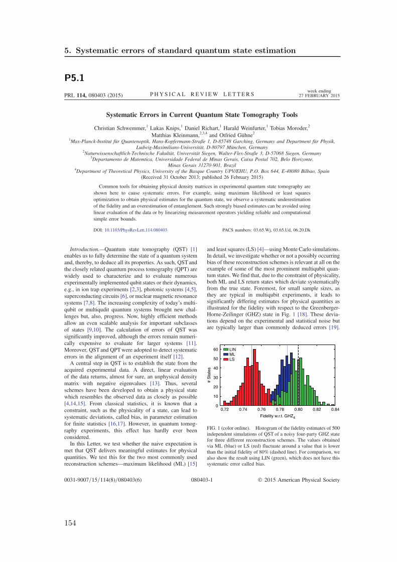
Systematic Errors in Current Quantum State Tomography Tools
Christian Schwemmer,1 Lukas Knips,1 Daniel Richart,1 Harald Weinfurter,1 Tobias Moroder,2
Matthias Kleinmann,2,3,4 and Otfried Gühne21Max-Planck-Institut für Quantenoptik, Hans-Kopfermann-Straße 1, D-85748 Garching, Germany and Department für Physik,
Ludwig-Maximilians-Universität, D-80797 München, Germany2Naturwissenschaftlich-Technische Fakultät, Universität Siegen, Walter-Flex-Straße 3, D-57068 Siegen, Germany
3Departamento de Matemtica, Universidade Federal de Minas Gerais, Caixa Postal 702, Belo Horizonte,Minas Gerais 31270-901, Brazil
4Department of Theoretical Physics, University of the Basque Country UPV/EHU, P.O. Box 644, E-48080 Bilbao, Spain(Received 31 October 2013; published 26 February 2015)
Common tools for obtaining physical density matrices in experimental quantum state tomography areshown here to cause systematic errors. For example, using maximum likelihood or least squaresoptimization to obtain physical estimates for the quantum state, we observe a systematic underestimationof the fidelity and an overestimation of entanglement. Such strongly biased estimates can be avoided usinglinear evaluation of the data or by linearizing measurement operators yielding reliable and computationalsimple error bounds.
DOI: 10.1103/PhysRevLett.114.080403 PACS numbers: 03.65.Wj, 03.65.Ud, 06.20.Dk
Introduction.—Quantum state tomography (QST) [1]enables us to fully determine the state of a quantum systemand, thereby, to deduce all its properties. As such, QST andthe closely related quantum process tomography (QPT) arewidely used to characterize and to evaluate numerousexperimentally implemented qubit states or their dynamics,e.g., in ion trap experiments [2,3], photonic systems [4,5],superconducting circuits [6], or nuclear magnetic resonancesystems [7,8]. The increasing complexity of today’s multi-qubit or multiqudit quantum systems brought new chal-lenges but, also, progress. Now, highly efficient methodsallow an even scalable analysis for important subclassesof states [9,10]. The calculation of errors of QST wassignificantly improved, although the errors remain numeri-cally expensive to evaluate for larger systems [11].Moreover, QST and QPTwere adopted to detect systematicerrors in the alignment of an experiment itself [12].A central step in QST is to establish the state from the
acquired experimental data. A direct, linear evaluationof the data returns, almost for sure, an unphysical densitymatrix with negative eigenvalues [13]. Thus, severalschemes have been developed to obtain a physical statewhich resembles the observed data as closely as possible[4,14,15]. From classical statistics, it is known that aconstraint, such as the physicality of a state, can lead tosystematic deviations, called bias, in parameter estimationfor finite statistics [16,17]. However, in quantum tomog-raphy experiments, this effect has hardly ever beenconsidered.In this Letter, we test whether the naive expectation is
met that QST delivers meaningful estimates for physicalquantities. We test this for the two most commonly usedreconstruction schemes—maximum likelihood (ML) [15]
and least squares (LS) [4]—using Monte Carlo simulations.In detail, we investigate whether or not a possibly occurringbias of these reconstruction schemes is relevant at all on theexample of some of the most prominent multiqubit quan-tum states. We find that, due to the constraint of physicality,both ML and LS return states which deviate systematicallyfrom the true state. Foremost, for small sample sizes, asthey are typical in multiqubit experiments, it leads tosignificantly differing estimates for physical quantities asillustrated for the fidelity with respect to the Greenberger-Horne-Zeilinger (GHZ) state in Fig. 1 [18]. These devia-tions depend on the experimental and statistical noise butare typically larger than commonly deduced errors [19].
10
20
30
40
50
setatS #
60
00.72 0.74 0.76 0.78 0.80 0.82 0.84
Fidelity w.r.t. GHZ4
LINMLLS
FIG. 1 (color online). Histogram of the fidelity estimates of 500independent simulations of QST of a noisy four-party GHZ statefor three different reconstruction schemes. The values obtainedvia ML (blue) or LS (red) fluctuate around a value that is lowerthan the initial fidelity of 80% (dashed line). For comparison, wealso show the result using LIN (green), which does not have thissystematic error called bias.
PRL 114, 080403 (2015) P HY S I CA L R EV I EW LE T T ER Sweek ending
27 FEBRUARY 2015
0031-9007=15=114(8)=080403(6) 080403-1 © 2015 American Physical Society
5. Systematic errors of standard quantum state estimation
P5.1
154

We demonstrate that, for linear quantities, one can providemeaningful confidence regions directly from the raw dataand that it is also possible to compute meaningful lower(upper) bounds on convex (concave) functions like thebipartite negativity.Standard state tomography tools.—The aim of QST is to
find an estimate together with some confidence region forthe initially unknown state ϱ0 of a system via appropriatemeasurements on multiple preparations of this state. Foran n-qubit system, the so-called Pauli tomography schemeconsists of measuring in the eigenbases of all 3n possiblecombinations of local Pauli operators, each yielding 2n
possible results [4]. In more general terms, in a tomographyprotocol, one repeats, for each measurement setting s, theexperiment a certain number of times Ns and obtains csrtimes the result r. These numbers then yield the frequenciesfsr ¼ csr=Ns. The probability to observe the outcome r forsetting s is given by Ps
ϱ0ðrÞ ¼ trðϱ0MsrÞ. Here, Ms
r labelsthe measurement operator corresponding to the result rwhen measuring setting s. The probabilities Ps
ϱ0ðrÞwill uni-quely identify the unknown state ϱ0, if the set of operatorsMs
r spans the space of traceless Hermitian operators.Provided the data f, i.e., the experimentally determined
frequencies fsr, one requires a method to determine theestimate ϱ≡ ϱðfÞ of the unknown state ϱ0. Simplyinverting the relations for Ps
ϱ0ðrÞ we obtain
ϱLIN ¼Xr;s
Asrfsr; ð1Þ
where Asr are determined from the measurement operators
Msr [8,20]. Note that there is a canonical construction of As
reven for the case of an overcomplete set ofMs
r, see SM 1 inthe Supplemental Material (SM) [21]. This reconstructionof ϱLIN is computationally simple and has become knownas linear inversion (LIN) [23]. In principle, Gaussianerror propagation could also be used here to determineconfidence regions.Yet, due to unavoidable statistical fluctuations, the
estimate ϱLIN is not a physical density operator for typicalexperimental situations; i.e., generally some eigenvaluesare negative. Apart from causing issues related to a physicalinterpretation of such a “state”, negative eigenvaluesimpedes the evaluation of interesting functions like thevon Neumann entropy, the quantum Fisher information, oran entanglement measure like the negativity, as thesefunctions are defined, or meaningful, only for valid, i.e.,positive semidefinite, quantum states.For this reason, different methods have been introduced
that mostly follow the paradigm that the reconstructed stateϱ ¼ argmaxϱ≥0TðϱjfÞ maximizes a target function TðϱjfÞwithin the set of valid density operators. This targetfunction, thereby, measures how well a density operatorϱ agrees with the observed data f. Two common choicesare ML [15] where TML ¼ P
r;sfsr log½Ps
ϱðrÞ�, and LS [4]where TLS ¼ −
Pr;s½fsr − Ps
ϱðrÞ�2=PsϱðrÞ. We denote the
respective optima by ϱML and ϱLS. From these estimates,one then easily computes any physical quantity of theobserved state, e.g., the fidelities FML ¼ hψ jϱMLjψi andFLS ¼ hψ jϱLSjψi with respect to the target state jψi.Numerical simulations.—To enable detailed analysis of
the particular features of the respective state reconstructionalgorithm and to exclude influence of systematic exper-imental errors, we perform Monte Carlo simulations.For a chosen state ϱ0, the following procedure is used:(i) Compute the single event probabilities Ps
ϱ0ðrÞ, (ii) tosscoins to get frequencies distributed according to themultinomial distribution determined by Ps
ϱ0ðrÞ and Ns,(iii) reconstruct the state with either reconstruction methodand compute the functions of interest, (iv) carry out steps(ii) and (iii) 500 times. Note that the optimality of themaximizations for ML and LS in step (iii) is certified byconvex optimization [10,24].First, we consider the four-qubit GHZ state jGHZ4i ¼
ðj0000i þ j1111iÞ= ffiffiffi2
pmixed with white noise, i.e., ϱ0 ¼
pjGHZ4ihGHZ4j þ ð1 − pÞ1=16 where p is chosen suchthat the fidelity is hGHZ4jϱ0jGHZ4i ¼ 0.8. This state is usedto simulate the Pauli tomography scheme. Figure 1 showsa typical histogram of the resulting fidelities for Ns ¼ 100measurement repetitions, which is a typical valueused for various multiqubit experiments. The fidelitiesobtained via LIN reconstruction fluctuate around theinitial value (FLIN ¼ 0.799� 0.012). (The values giventhere are the mean and the standard deviation obtainedfrom the 500 reconstructed states). In stark contrast, bothML (FML ¼ 0.788� 0.010) and even more LS (FLS ¼0.749� 0.010) systematically underestimate the fidelity,i.e., are strongly biased. Evidently, the fidelities of thereconstructed states differ bymore than 1 standard deviationfor ML and even more than 5 standard deviations for LS.The question of how these systematic errors depend on theparameters of the simulation arises. Let us start by inves-tigating the dependence on the number of repetitions Ns.Figure 2(a) shows the mean and the standard deviationsof histograms like the one shown in Fig. 1 for different Ns.As expected, the systematic errors are more profound forlow numbers of repetitions Ns per setting s and decreasewith increasingNs. Yet, even forNs ¼ 500, a number hardlyused in multiqubit experiments, FLS still deviates by 1standard deviation from the value for the initial state. Theeffect is also, by no means, special for the GHZ state butwas equally observed for other prominent four-party states,here, also, chosen with a fidelity of 80%, see Figs. 2(b)–2(d)and the SM [21].The systematic deviations also vary with the number of
qubits or the purity of the initial state. Figure 3(a) shows therespective dependencies of the fidelity for n-qubit statesϱ0 ¼ pjGHZnihGHZnj þ ð1 − pÞ1=2n (for Ns ¼ 100).Here, a significant increase of the bias with the numberof qubits is observed especially for LS. Also, when varyingthe purity or fidelity with the GHZ state, respectively,
PRL 114, 080403 (2015) P HY S I CA L R EV I EW LE T T ER Sweek ending
27 FEBRUARY 2015
080403-2
5.3. Publications
155

we observe a large deviation for ML and LS estimators[Fig. 3(b)]. If the initial fidelity is very low, the effect isnegligible, but large fidelity values suffer from strongerdeviations, especially for LS.The reliability of the estimates ϱ or of physical quantities
deduced thereof are quantified by the size of confidenceregions which commonly are deduced by bootstrappingmethods [19]. Starting either from the estimate ϱEST(EST ∈ fML;LSg) or the observed data set f, this erroris typically accessed by Monte Carlo sampling: Onerepeatedly simulates data fðiÞ according to the state ϱESTor f together with a reasonable noise model for therespective experiment and reconstructs the state ϱðfðiÞÞ.From the resulting empirical distribution, one then reportsthe standard deviation (or a region including, say, 68%of the simulated states) for the matrix elements or forquantities of interest [19], see also SM 3. However, theproblem with such error regions is that they are typicallytoo small since they reflect only statistical fluctuations of
the biased estimate, which can easily be smaller than thesystematic error [26].In summary, we observe systematic errors, which depend
on the state reconstruction method and the strength of thestatistical fluctuations of the count rates. Any manualcorrection of the bias and the statistical fluctuations [17]seems out of reach, since the effect depends on theunknown initial state which cannot be calculated fromthe observed data [16]. Let us emphasize that in most casesthe initial value differs by more than the statistical errordetermined via bootstrapping (cf. SM 3 [21]).Biased and unbiased estimators.—The systematic offset
discussed above is well known in the theory of pointestimates [26]. Expressed for QST, an estimator ϱ is calledunbiased if its fluctuations are centered around the truemean, such that, for its expectation value,
Eϱ0ðϱÞ≡Xf
Pϱ0ðfÞϱðfÞ ¼ ϱ0 ð2Þ
holds for all possible states ϱ0 with Pϱ0ðfÞ the probabilityto observe the data f. An estimator that violates Eq. (2) iscalled biased. Similar definitions hold, for instance, forfidelity estimators, Eϱ0ðFÞ ¼ hψ jϱ0jψi≡ F0. This termi-nology is motivated by the form of the mean squared error,which decomposes, for example, for the fidelity into
Eϱ0 ½ðF − F0Þ2� ¼ Vϱ0ðFÞ þ ½Eϱ0ðFÞ − F0�2; ð3Þ
where VðFÞ≡ EðF2Þ − EðFÞ2 denotes the variance.Equation (3) consists of two conceptually different parts.The first is a statistical term quantifying the fluctuations ofthe estimator F itself. The second, purely systematic term,is called bias and vanishes for unbiased estimators [27].Note that, since the expectation values of the frequenciesare the probabilities, Eϱ0ðfsrÞ ¼ Ps
ϱ0ðrÞ, and because ϱLIN asgiven by Eq. (1) is linear in fsr, the determination of aquantum state using LIN is unbiased. However, as shownbelow, for QST, the bias is inherent to estimators con-strained to giving only physical answers.Proposition.—A reconstruction scheme for QST that
always yields valid density operators is biased.Proof.—For a tomography experiment on the state jψ ii
with finite measurement time, there is a set of possible dataSi ¼ ffijPjψ iiðfiÞ > 0g, with Pjψ iiðfiÞ the probability toobtain data fi when observing state jψ ii.Consider two pure nonorthogonal states jψ1i and jψ2i
(hψ1jψ2i ≠ 0). For these two states, there exists a nonemptyset of data S12 ¼ ff0jPjψ1iðf0Þ · Pjψ2iðf0Þ > 0g ¼ S1∩S2,which can occur for both states.Now, let us assume that a reconstruction scheme ϱ
provides a valid quantum state ϱðfÞ for all possibleoutcomes f and that Eq. (2) is satisfied for jψ1i, i.e.,P
S1Pjψ1iðf1Þϱðf1Þ ¼ jψ1ihψ1j. This incoherent sum over
all ϱðf1Þ can be equal to the pure state jψ1ihψ1j only for the
10010
Events per Setting
100 000101
etatS tegraT .t.r.
w ytilediF
0.70
0.75
0.85
0.80
0.65
D State+ white Noise
4(2)
0.70
0.75
0.85
0.80
GHZ4 State+ white Noise
(a)
(c)
Cluster State+ white Noise
(b)
Smolin State+ white Noise
LINMLLS
(d)
FIG. 2 (color online). The performance of ML, LS, and LINmethods depending on the number of events Ns per setting andfor four different noisy initial states ϱ0. Note that the fidelity canonly be calculated linearly if the reference state is pure which isnot the case for the Smolin state [25]. Therefore, only the curvesfor ML and LS are plotted for the Smolin state.
-0.06
-0.02
0
0.04
0.02ZH
G .t.r.w ytiledi
F
32 4 5Number of Qubits
6
GHZ States + white Noise, F=0.80
0.60.0625 0.8Fidelity of 0
0.4
saiB ytile di
F
1.0
GHZ4 + white Noise
-0.04
0.60
0.70
0.75
0.85
0.80
0.65
-0.08
LINMLLS
(a) (b)
0.2
FIG. 3 (color online). The behavior of ML, LS, and LINdepending on the number of qubits n (left) and the fidelity ofϱ0 (right).
PRL 114, 080403 (2015) P HY S I CA L R EV I EW LE T T ER Sweek ending
27 FEBRUARY 2015
080403-3
5. Systematic errors of standard quantum state estimation
156

(already pathological) case that ϱðf1Þ ¼ jψ1ihψ1j for allf1 ∈ S1. This means that the outcome of the reconstructionis fixed for all f1 including all data f0 ∈ S12. As thesedata also occur for state jψ2i, there exist f2 ∈ S12 withϱðf2Þ ¼ jψ1ihψ1j ≠ jψ2ihψ2j. Thus, in Eq. (2), the sumover all reconstructed states now is an incoherentmixture of at least two pure states, and the conditionP
S2Pjψ2iðf2Þϱðf2Þ ¼ jψ2ihψ2j is violated for jψ2i. Hence,
ϱ does not obey Eq. (2) for jψ2i and is, therefore,biased [28].This leaves us with the tradeoff: Should one necessarily
use an algorithm like ML or LS to obtain a valid quantumstate but suffer from a bias, or should one use LIN whichis unbiased but typically delivers an unphysical result?In the following, we propose a scheme using linearizedoperators to provide a valid, lower or upper bound andan easily computable confidence region for many quantitiesof interest.Parameter estimation by linear evaluation.—Many rel-
evant functions are either convex, like most entanglementmeasures or the quantum Fisher information, or concave,like the von Neumann entropy. Thus, these operators can belinearized around some properly chosen state in order toobtain a reliable lower (upper) bound. Note that, typically,a lower bound on an entanglement measure is often suitedfor evaluating experimental states, whereas an upper bounddoes not give much additional information.Recall that a differentiable function gðxÞ is convex if
gðxÞ ≥ gðx0Þ þ∇gðx0ÞTðx − x0Þ holds for all x; x0. In ourcase, we are interested in a function gðxÞ ¼ g½ϱðxÞ� where xis a variable to parametrize a quantum state ϱ in a linearway. From convexity, it follows that it is possible to find anoperator L, such that
trðϱ0LÞ ≤ gðϱ0Þ ð4Þholds for all ϱ0 (similarly an upper bound is obtained forconcave functions). This operator L can be determinedfrom the derivatives of gðxÞ with respect to x at a suitablepoint x0, from the Legendre transformation [29], or directlyinferred from the definition of the function gðxÞ [30].A detailed discussion is given in SM 5 [21].For this bound, a confidence region, i.e., the error region
for the frequentistic approach, can be calculated. Forexample, a one-sided confidence region of level γ canbe described by a function C on the data f such thatProbϱ0 ½C ≤ gðϱ0Þ� ≥ γ holds for all ϱ0 [26]. According toHoeffding’s tail inequality [31] and a given decompositionof L ¼ P
lsrMsr into the measurement operators Ms
r, aconfidence region, then, is
C ¼ trðϱLINLÞ −ffiffiffiffiffiffiffiffiffiffiffiffiffiffiffiffiffiffiffiffiffiffiffiffiffiffiffiffih2j logð1 − γÞj
2Ns
s; ð5Þ
where h2 is given by h2 ¼ Psðlsmax − lsminÞ2, and lsmax =min
denotes the respective extrema of lsr over r for each
setting s. Although not optimal, such error regions areeasy to evaluate and valid without extra assumptions.Since we directly compute a confidence region on gðxÞ,we obtain, generally, a tighter result than what would beobtained from a “smallest” confidence region on densityoperators which tend to drastically overestimate the error(see SM 4 [21] for an example).In the following, we show how to use a linearized
operator on the example of the bipartite negativity [30].(For the quantum Fisher information [32] and additionaldiscussion, see SM 5 [21].) A lower bound on thenegativity NðϱABÞ of a bipartite state ϱAB is given byNðϱABÞ ≥ trðϱABLÞ for any L satisfying 1 ≥ LTA ≥ 0,where the superscript TA denotes partial transposition[33] with respect to party A. This bound is tight if L isthe projector on the negative eigenspace of ϱTA
AB. Using thislinear expression, one can directly compute the lowerbound on the negativity and, by using Eq. (5), the one-sided confidence region. Any choice of L is, in principle,valid, but, for a good performance, L should be chosenaccording to the experimental situation. We assume, how-ever, no prior knowledge and rather estimate L independentof the tomographic data by the projection on the negativeeigenspace of ϱTA
ML deduced from an additional tomography,again withNs ¼ 100 counts per setting. One can, of course,also start with an educated guess of L motivated by thetarget state one wants to prepare.Figure 4 shows the distributions of the negativity
between qubits A ¼ f1; 2g and B ¼ f3; 4g for the four-qubit GHZ state and for the separable four-qubit statejψ sepi ∝ ðj0i þ jþiÞ⊗4, with jþi∝ ðj0iþ j1iÞ, each mixedwith white noise such that the fidelity with the respectivepure state is 80%. In both cases, we observe that ML andLS overestimate the amount of entanglement. Even if noentanglement is present, ML and LS clearly indicateentanglement. In contrast, the lower bound of the negativitydoes not indicate spurious entanglement. As negativity
Bipartite Negativity
0.450.35 0.400.300.25
LBLMLLS
20
40
setatS #
60
80
0
separable State + white NoiseGHZ4 State + white Noise
0.05 0.10-0.05 0-0.100.20
100
120
FIG. 4 (color online). Lower bound obtained by linearizingbipartite negativity (LBL) for the GHZ (left) and a four-qubitproduct state (right) both mixed with white noise resulting in 80%fidelity. The ML and LS reconstruction leads to a systematicoverestimation of the negativity, while the lower bound yields avalid estimate.
PRL 114, 080403 (2015) P HY S I CA L R EV I EW LE T T ER Sweek ending
27 FEBRUARY 2015
080403-4
5.3. Publications
157

gives lower bounds of other entanglement measures, thosewould overestimate entanglement of a state, too [34].Conclusion.—Any state reconstruction algorithm enforc-
ing physicality of the result suffers from systematic devia-tions. We have shown that, for the commonly used methods,this bias is significant for data sizes typical in currentexperiments. Quantities that are computed from such a pointestimate can easily inherit this bias and lead to erroneousconclusions, as shown here on the examples of the fidelity,the negativity, and the Fisher information. Equivalentstatements can be inferred for process tomography.Recently, methods have been used to obtain confidence
regions via the likelihood function. However, these arenotoriously difficult to compute. The linearization methoddeveloped here yields a well defined confidence regionfor interesting quantities. This quantity is easily calculable,yet pessimistic. The quest is, thus, open for finding tighter,but still computationally accessible, confidence regions.
We would like to thank P. Drummond, B. Englert, D.Gross, H. K. Ng, M. Raymer, and J. Shang for stimulatingdiscussions. This work has been supported by the EU(Marie Curie CIG 293993/ENFOQI, ERC Starting GrantGEDENTQOPT, FET Project QWAD, ERC QOLAPS), theBMBF (Chist-Era Project QUASAR), the Brazilian agencyCAPES, through the program Science without Borders, andthe Elite Network of Bavaria (PhD programs QCCCand ExQM).
[1] Quantum State Estimation, edited by M. G. A. Paris andJ. Řeháček, (Springer, Berlin, 2004).
[2] H. Häffner, W. Hänsel, C. F. Roos, J. Benhelm, D. Chek-al-kar, M. Chwalla, T. Körber, U. D. Rapol, M. Riebe, P. O.Schmidt et al., Nature (London) 438, 643 (2005).
[3] J. P. Home, D. Hanneke, J. D. Jost, J. M. Amini, D.Leibfried, and D. J. Wineland, Science 325, 1227 (2009);J. P. Gaebler, A. M. Meier, T. R. Tan, R. Bowler, Y. Lin,D. Hanneke, J. D. Jost, J. P. Home, E. Knill, D. Leibfried,and D. J. Wineland, Phys. Rev. Lett. 108, 260503 (2012).
[4] D. F. V. James, P. G. Kwiat, W. J. Munro, and A. G. White,Phys. Rev. A 64, 052312 (2001).
[5] K. J. Resch, P. Walther, and A. Zeilinger, Phys. Rev. Lett.,94, 070402 (2005); N. Kiesel, C. Schmid, G. Tóth, E.Solano, and H. Weinfurter, Phys. Rev. Lett. 98, 063604(2007); M.W. Mitchell, C. W. Ellenor, S. Schneider, andA.M. Steinberg, Phys. Rev. Lett. 91, 120402 (2003).
[6] L. DiCarlo, J. M. Chow, J. M. Gambetta, L. S. Bishop, B. R.Johnson, D. I. Schuster, A. Majer, J. Blais, L. Frunzio, S. M.Girvin, and R. J. Schoelkopf, Nature (London) 460, 240(2009); M. Neeley, R. C. Bialczak, M. Lenander, E. Lucero,M. Mariantoni, A. D. O’Connell, D. Sank, H. Wang, M.Weides, J. Wenner et al., Nature (London) 467, 570 (2010);A. Fedorov, L. Steffen, M. Baur, M. da Silva, andA. Wallraff, Nature (London) 481, 170 (2012); J. M. Chow,J. M. Gambetta, A. D. Córcoles, S. T. Merkel, J. A. Smolin,C. Rigetti, S. Poletto, G. A. Keefe, M. B. Rothwell,
J. R. Rozen, M. B. Ketchen, and M. Steffen, Phys. Rev.Lett. 109, 060501 (2012).
[7] O. Mangold, A. Heidebrecht, and M. Mehring, Phys. Rev. A70, 042307 (2004); M. A. Nielsen, E. Knill, and R.Laflamme, Nature (London) 396, 52 (1998).
[8] I. L. Chuang andM.A.Nielsen, J.Mod.Opt. 44, 2455 (1997).[9] D. Gross, Y.-K. Liu, S. T. Flammia, S. Becker, and J.
Eisert, Phys. Rev. Lett. 105, 150401 (2010); G. Tóth, W.Wieczorek, D. Gross, R. Krischek, C. Schwemmer, andH. Weinfurter, Phys. Rev. Lett. 105, 250403 (2010); M.Cramer, M. B. Plenio, S. T. Flammia, D. Gross, S. D.Bartlett, R. Somma, O. Landon-Cardinal, Y.-K. Liu, andD. Poulin, Nat. Commun. 1, 149 (2010); O. Landon-Cardinal and D. Poulin, New J. Phys. 14, 085004 (2012).
[10] T. Moroder, P. Hyllus, G. Tóth, C. Schwemmer, A.Niggebaum, S. Gaile, O. Gühne, and H. Weinfurter, NewJ. Phys. 14, 105001 (2012).
[11] M. Christandl and R. Renner, Phys. Rev. Lett. 109, 120403(2012); T. Sugiyama, P. S. Turner, and M. Murao,Phys. Rev. Lett. 111, 160406 (2013); R. Blume-Kohout,arXiv:1202.5270; J. Shang, H. K. Ng, A. Sehrawat, X. Li,and B.-G. Englert, New J. Phys. 15, 123026 (2013).
[12] T. Moroder, M. Kleinmann, P. Schindler, T. Monz, O.Gühne, and R. Blatt, Phys. Rev. Lett. 110, 180401 (2013);D. Rosset, R. Ferretti-Schöbitz, J.-D. Bancal, N. Gisin, andY.-C. Liang, Phys. Rev. A 86, 062325 (2012); C. Stark,Phys. Rev. A 89, 052109 (2014); N. K. Langford, New J.Phys. 15, 035003 (2013); S. J. van Enk and R. Blume-Kohout, New J. Phys. 15, 025024 (2013); S. T. Merkel,J. M. Gambetta, J. A. Smolin, S. Poletto, A. D. Córcoles,B. R. Johnson, C. A. Ryan, and M. Steffen, Phys. Rev. A 87,062119 (2013).
[13] D. Smithey, M. Beck, M. G. Raymer, and A. Faridani,Phys. Rev. Lett. 70, 1244 (1993); G. M. D’Ariano, C.Macchiavello, and N. Sterpi, Quantum Semiclass. Opt. 9,929 (1997); U. Leonhardt, M. Munroe, T. Kiss, T. Richter,and M. Raymer, Opt. Commun. 127, 144 (1996).
[14] R. Blume-Kohout, New J. Phys. 12, 043034 (2010); Phys.Rev. Lett. 105, 200504 (2010).
[15] Z. Hradil, Phys. Rev. A 55, R1561 (1997).[16] T. Sugiyama, P. S. Turner, and M. Murao, New J. Phys. 14,
085005 (2012).[17] C.W. Helstrom, Phys. Lett., 25A, 101 (1967); S. L.
Braunstein andC.M.Caves, Phys. Rev. Lett. 72, 3439 (1994).[18] We stress that ML methods can, in principle, be used
for directly estimating the fidelity without reconstructingthe quantum state, but most experiments using ML firstreconstruct the state and then calculate the fidelity. Thisprocedure is the subject of our criticism.
[19] B. Efron and R. J. Tibshirani, An Introduction to theBootstrap (Chapman & Hall, London, 1994).
[20] J. F. Poyatos, J. I. Cirac, and P. Zoller, Phys. Rev. Lett. 78,390 (1997); N. Kiesel, Ph.D. thesis, Ludwig-Maximilians-Universität München, 2007; T. Kiesel, Phys. Rev. A 85,052114 (2012).
[21] See Supplemental Material at http://link.aps.org/supplemental/10.1103/PhysRevLett.114.080403 for detailson LIN, additional examples of states with a strong bias,examples for bootstrapping, the difference between multi-parameter and scalar confidence regions, and further details
PRL 114, 080403 (2015) P HY S I CA L R EV I EW LE T T ER Sweek ending
27 FEBRUARY 2015
080403-5
5. Systematic errors of standard quantum state estimation
158
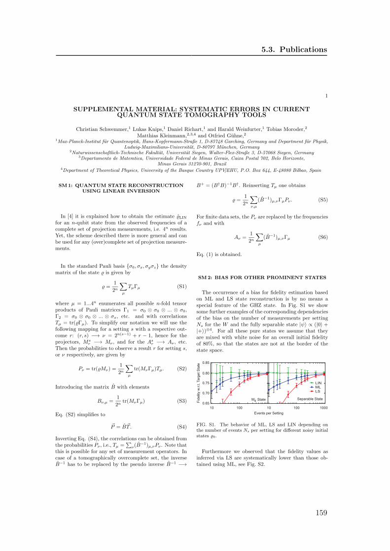
1
SUPPLEMENTAL MATERIAL: SYSTEMATIC ERRORS IN CURRENTQUANTUM STATE TOMOGRAPHY TOOLS
Christian Schwemmer,1 Lukas Knips,1 Daniel Richart,1 and Harald Weinfurter,1 Tobias Moroder,2
Matthias Kleinmann,2,3,4 and Otfried Guhne,21Max-Planck-Institut fur Quantenoptik, Hans-Kopfermann-Straße 1, D-85748 Garching, Germany and Department fur Physik,
Ludwig-Maximilians-Universitat, D-80797 Munchen, Germany2Naturwissenschaftlich-Technische Fakultat, Universitat Siegen, Walter-Flex-Straße 3, D-57068 Siegen, Germany
3Departamento de Matemtica, Universidade Federal de Minas Gerais, Caixa Postal 702, Belo Horizonte,Minas Gerais 31270-901, Brazil
4Department of Theoretical Physics, University of the Basque Country UPV/EHU, P.O. Box 644, E-48080 Bilbao, Spain
SM1: QUANTUM STATE RECONSTRUCTIONUSING LINEAR INVERSION
In [4] it is explained how to obtain the estimate %LINfor an n-qubit state from the observed frequencies of acomplete set of projection measurements, i.e. 4n results.Yet, the scheme described there is more general and canbe used for any (over)complete set of projection measure-ments.
In the standard Pauli basis {σ0, σx, σyσz} the densitymatrix of the state % is given by
% =1
2n
∑µ
TµΓµ (S1)
where µ = 1...4n enumerates all possible n-fold tensorproducts of Pauli matrices Γ1 = σ0 ⊗ σ0 ⊗ ... ⊗ σ0,Γ2 = σ0 ⊗ σ0 ⊗ ... ⊗ σx, etc. and with correlationsTµ = tr(%Γµ). To simplify our notation we will use thefollowing mapping for a setting s with a respective out-come r: (r, s) −→ ν = 2n(s−1) + r − 1, hence for theprojectors, Ms
r −→ Mν , and for the Asr −→ Aν , etc.Then the probabilities to observe a result r for setting s,or ν respectively, are given by
Pν = tr(%Mν) =1
2n
∑µ
tr(MνΓµ)Tµ. (S2)
Introducing the matrix B with elements
Bν,µ =1
2ntr(MνΓµ) (S3)
Eq. (S2) simplifies to
~P = B ~T . (S4)
Inverting Eq. (S4), the correlations can be obtained fromthe probabilities Pν , i.e., Tµ =
∑ν(B−1)µ,νPν . Note that
this is possible for any set of measurement operators. Incase of a tomographically overcomplete set, the inverseB−1 has to be replaced by the pseudo inverse B−1 −→
B+ = (B†B)−1B†. Reinserting Tµ one obtains
% =1
2n
∑ν,µ
(B−1)µ,νΓµPν . (S5)
For finite data sets, the Pν are replaced by the frequenciesfν and with
Aν =1
2n
∑µ
(B−1)µ,νΓµ (S6)
Eq. (1) is obtained.
SM2: BIAS FOR OTHER PROMINENT STATES
The occurrence of a bias for fidelity estimation basedon ML and LS state reconstruction is by no means aspecial feature of the GHZ state. In Fig. S1 we showsome further examples of the corresponding dependenciesof the bias on the number of measurements per settingNs for the W and the fully separable state |ψ〉 ∝ (|0〉 +|+〉)⊗4. For all these pure states we assume that theyare mixed with white noise for an overall initial fidelityof 80%, so that the states are not at the border of thestate space.
0.70
0.75
0.85
0.80
0.65Fid
elit
y w
.r.t.Ta
rget
Sta
te
10 100
Events per Setting
10 100 1000
LINML
LS
W State4Separable State
FIG. S1. The behavior of ML, LS and LIN depending onthe number of events Ns per setting for different noisy initialstates %0.
Furthermore we observed that the fidelity values asinferred via LS are systematically lower than those ob-tained using ML, see Fig. S2.
5.3. Publications
159

2
100
50
0-0.08 -0.06 -0.04 -0.02 0 0.02 0.04
# S
tate
s
ML-LIN
LS-LIN
LS-ML
Differences
FIG. S2. Here we show the differences of the respective fidelityestimates evaluated for each single simulated tomography ex-periment as shown in Fig. 1 of the main text. It shows thatthe respective ML or LS estimate, with one rare exception,is always lower than the LIN estimate. Comparing ML andLS (gray) shows that not only on average but also for everysingle data set LS delivers a smaller fidelity value than ML.
SM3: BOOTSTRAPPING
As already mentioned in the main text, in many pub-lications where QST is performed the standard error baris calculated by bootstrapping based on Monte Carlomethods. One can here distinguish between paramet-ric bootstrapping, where f (i) are sampled according toP s(r) = tr(%(fobs)M
sr ), and non-parametric bootstrap-
ping, where P s(r) = fobs is used instead.
We consider again the four-qubit GHZ state of 80%fidelity and Ns = 100. Interpreting the simulations ofFig. 1 as Monte-Carlo simulations from the parametricbootstrap with P s(r) = tr(%0M
sr ) we have already seen
that ML and LS yield fidelity estimates below the actualvalue. If one uses now one of these data sets fobs as aseed to generate new samples f (i) the fidelity decreasesfurther. As shown in Fig. S3 this happens in particularfor parametric bootstrapping (0.777± 0.011 for ML and0.700±0.012 for LS) while non-parametric bootstrapping(0.780± 0.011 for ML and 0.714± 0.012 for LS) weakensthis effect. However, in this context, one is interested infact in the standard deviation of the simulated distribu-tion. In our simulations it is somewhat smaller than thedistribution of linearly evaluated fidelities. This means,the biasedness of ML and LS methods leads to a falseestimate of the error, too.
SM4: CONFIDENCE REGIONS FOR STATESVS. SCALAR QUANTITIES
Let us now comment on confidence regions (CR) fordensity operators and CR on parameter functions Q.Having a (tractable) method to compute CR for statesC%(f) [11], one could think that this region of states alsoprovides good CR for the parameter functions Q, if onemanages to evaluate the minimal and maximal values ofQ(%) for all % ∈ C%(f). However, such CR are typicallymuch worse than CR evaluated for Q directly, the reasonbeing the large freedom in how to build up a CR. Let us
give the following illustrative example, see also Fig. S4:
Let us consider the task to obtain a CR for the twomean values ~µ = (µ1, µ2) of two independent Gaussianexperiments, where the firstN samples xi are drawn fromN (µ1, σ
2) while the remaining N instances yi originatefrom N (µ2, σ
2), both with the same known variances. Ifone is interested in an 68% CR for both mean values ~µthen both possible recipes
C(1) = {~µ : ‖~µ− (x, y)‖ ≤ 1.52σ/√N}, (S7)
C(2) = [x− σ/√N, x+ σ/
√N ]× (−∞,∞) (S8)
with x = 1N
∑i xi and similar for y are valid 68% CR.
However, while C(1) yields the smallest area for the CR, itgives a much larger confidence region for Q(~µ) = µ1 thanif we would directly use C(2), which in fact is the smallestone for µ1. Note that this effect increases roughly with√
dim if one adds further parameters in the consideredGaussian example. Therefore we see that “errors” asso-ciated with CR on the density operator are not the bestchoice if one is interested only on a few key properties ofthe state.
0.720.68 0.76
Fidelity w.r.t. GHZ4
# S
tate
s
10
20
30
40
50
60
0
10
20
30
40
50
70
60
0
Non-Parametric BootstrappingParametric Bootstrapping
ML
before BSafter BS
0.720.68 0.76 0.800.80
FLS
FIG. S3. Error bar computation for the fidelity of the four-qubit GHZ state via Monte-Carlo simulation using eitherparametric or non-parametric bootstrapping with the datafrom Fig. 1. For each of these 500 observations fobs, 100 newdata sets f (i) were generated and reconstructed in order todeduce the mean and standard deviation as an error bar forthe fidelity. The histograms denoted by “after BS” show thedistributions of these means together with an averaged errorbar given by the gray shaded areas. The initial values for thefidelities are described by the dashed lines.
5. Systematic errors of standard quantum state estimation
160

3
μ
μ2
μ
μ2
μ1.521 1
Smallest 68% CR ( 1, 2) Smallest 68% CR 1
FIG. S4. Which confidence region is the smallest? If oneis interested in both mean values ~µ = (µ1, µ2) then clearlythe left one represents the smallest one, but if Q(~µ) = µ1 ischosen, then the CR obtained by projection onto theµ1-axisis much larger for the disc-shaped area.
SM5: BOUNDS ON CONVEX/CONCAVEFUNCTIONS
As mentioned in the main text, one can directly boundconvex (or concave) functions g(x) by linear ones usingan operator L
tr(%0L) ≤ g(%0). (S9)
Here, we want to explain in detail how the operatorL can be determined from the derivatives of g[%(x)].Therefore, we parametrize the density operator %(x) =11/ dim +
∑i xiSi via an orthonormal basis Si of Her-
mitian traceless operators. A possible choice for theSi are all normalized traceless tensor products of thePauli matrices and the identity. Since we employ anaffine parametrization, the function g(x) = g[%(x)] is con-vex. Direct calculation shows that choosing the operatorL[%(x′)] = l011 +
∑i liSi as
l0 = g[%guess(x′)]−
∑i
x′i∂
∂xig[%guess(x
′)] (S10)
li =∂
∂xig[%guess(x
′)] (S11)
gives due to the convexity condition g(x) ≥ g(x′) +∇g(x′)T (x − x′) a lower bound as in Eq. (S9). Here,L[%(x′)] is computed on a “guess” x′, i.e., %guess(x
′) ofthe true state %0. Recall that while the guess %guess mustbe a valid state the lower bound tr(%0L) is well-definedalso for nonphysical density operators.
As an example how to apply this linearization, letus consider the quantum Fisher information f(x) =F (%,H), which measures the suitability of a state % todetermine the parameter θ in an evolution U(θ,H) =
LBLIN
109 11
Fisher Information w.r.t. Jz
# S
tate
s
10
20
30
40
50
70
60
0
10
20
30
40
50
70
60
80
0
Non-Parametric BootstrappingParametric Bootstrapping
ML
1312
FLS
10 11 1312 1414
before BSafter BS
FIG. S5. Full analysis of a Pauli QST scheme with Ns = 100on four qubits in order to deduce the quantum Fisher infor-mation with respect to H = Jz. As the true underlying statewe assume again a noisy four-party GHZ state. We observethat the quantum Fisher information is underestimated fromboth ML and LS, while the lower bound deduced from LIN isfine.
e−iθH . More explicitly the formulae are given by
f(x) = 2∑jk
(λj − λk)2
λj + λkHjkHkj , (S12)
∂
∂xif(x) = 4
∑jkl
λjλk + λjλl + λkλl − 3λ2j(λj + λk)(λj + λl)
HjkSi,klHlj
(S13)
where {λi, |ψi〉} denotes the eigenspectrum of %(x),Hjk = 〈ψj |H|ψk〉 and Si,kl = 〈ψk|Si|ψl〉. In order tocompute the derivative of the Fisher information onecan employ the alternative form, as given for instancein Ref. [32],
F (%,H) = tr[(H%2 + %2H − 2%H%)J−1% (H)], (S14)
J−1% (H) =
∫ ∞0
dt e−t/2%He−t/2%. (S15)
such that the derivative can be computed via the help ofmatrix derivatives [22].
Now let us imagine that we want to determine thequantum Fisher information of a four-qubit state withrespect to H = Jz, while our true underlying state %0is once more the noisy GHZ state of 80% fidelity. Fig-ure S5 shows the full simulation of a Pauli tomographyexperiment with Ns = 100 together with the standarderror analysis using parametric or non-parametric boot-strapping. As with the other examples, we observe a sys-tematic discrepancy between the results of standard QSTtools and the true value. In this case, though the quan-tum Fisher information is typically larger for stronger
5.3. Publications
161

4
entangled states, ML or LS underestimate the true ca-pabilities of the state. However, if we use the describedmethod for LIN (with an in this case optimized operatorL) the lower bound via LIN is fine.
For completeness, we also give the respective deriva-tives for further convex functions of interest like the pu-rity g(x) = tr(%2)
∂
∂xig(x) = 2 tr[Si%(x)] (S16)
and correspondingly for the von Neumann entropy
g(x) = − tr(% log %)
∂
∂xig(x) = − tr[Si(log %(x))]. (S17)
[4] D. F. V. James, P. G. Kwiat, W. J. Munro, and A. G.White, Phys. Rev. A 64, 052312 (2001).
[11] M. Christandl and R. Renner, Phys. Rev. Lett. 109,120403 (2012); T. Sugiyama, P. S. Turner, and M. Murao,Phys. Rev. Lett. 111, 160406 (2013); R. Blume-Kohout,arXiv:1202.5270; J. Shang, H. K. Ng, A. Sehrawat, X. Li,and B.-G. Englert, New J. Phys. 15, 123026 (2013).
[22] R. A. Horn and C. R. Johnson, Topics in matrix analysis(Cambridge University Press, 1991).
[32] D. Petz and C. Ghinea, QP–PQ: Quantum Probab.White Noise Anal. 27, 261 (2011).
5. Systematic errors of standard quantum state estimation
162

6. Conclusions
In the present thesis, highly efficient novel tools for entanglement detection andthe tomographic analysis of genuinely multipartite entangled quantum states werepresented. These tools were experimentally implemented on the example of vari-ous multiqubit states with up to six photons. The focus of this research work wastwofold: First, the emphasis was on the development and application of experi-mentally friendly entanglement indicators which allow for conclusive statementsabout the presence of entanglement from possibly few measurements. In this con-text, it was also investigated which types of correlations are actually necessaryfor genuine N -partite entanglement. Second, new approaches for partial quantumstate tomography were studied. For the experimental implementation of theseschemes, and in order to compare them against full state tomography, it was nec-essary to further increase the pump power of the photon source and to improvethe efficiency of the whole optical setup.
Many entanglement criteria that are state independent require knowledge of thecomplete density matrix and are therefore experimentally costly. In contrast, othercriteria, like entanglement witnesses, are experimentally far more friendly in termsof the measurement effort but dependent on the state to be investigated. Ideally,an entangled criterion should be, at the same time, state independent and requireonly few measurements. In this work, two schemes for fast entanglement detectionwere presented that are both state independent and do not require a full statetomography [52, 53] (see publications P3.1 and P3.2). The first scheme is designedfor pure two-qubit states and consists of two steps. In the first step, the localSchmidt bases are determined and the state is (up to a phase) transformed into theSchmidt basis. Then, in the second step, entanglement can easily be verified witha simple criterion [51] which requires at maximum three correlation measurements.The second scheme is based on the principle of correlation complementarity [63]and can also be applied for states with more than two qubits. It can be expressedin a compact form called decision tree which optimally reflects the adaptivity ofthe scheme, i.e., the result of the previous correlation measurement determineswhich is the next measurement to be carried out.
The approach to use correlation measurements to detect entanglement was alsoapplied to a particular three-qubit state [54] (see publication P3.3). Generally,entanglement criteria that are used to verify N -partite genuine entanglement de-pend on N -partite correlations [51, 60, 64–71]. However, interestingly, quan-tum mechanics allows for states that are genuinely N -partite entangled without
163

6. Conclusions
N -partite correlations [74]. In this work, a general scheme was presented to con-struct quantum states with vanishing N -partite correlations for an odd numberof qubits. In order to characterize such remarkable states, two experiments aim-ing at the preparation of symmetric Dicke states with four and six qubits werecarried out. The target states could then be obtained by performing appropriateprojection measurements [127].
In case one wants to gain more information about a quantum state than justwhether it is entangled or not but full tomography is unwanted or not feasible, theapplication of a partial tomography scheme is the method of choice. In the presentwork, two novel schemes for partial tomography schemes, compressed sensing andpermutationally invariant tomography, were discussed. They were both experi-mentally implemented to characterize symmetric Dicke states with four and sixphotons [56, 58] (see publications P4.1 and P4.2). In these experiments, it couldbe shown that full tomography and permutationally invariant tomography delivercompatible results. For the analysis of six qubits, it could be shown that the ex-perimental effort in comparison to full tomography could be reduced considerably.In detail, the effort could be reduced by a factor of 3 for compressed sensing, by afactor of 25 for permutationally invariant tomography, and by a factor of 50 for acombination of the two methods. In this context, it is also highly important thatone has efficient algorithms for data analysis at hand [57] (see P4.3). Therefore,a novel algorithm based on convex optimization was applied.
For every experiment, a careful analysis of all the errors that might influencethe final result is required. In this work, it was investigated whether the standardapproach for data post processing itself can lead to systematic errors [59] (seepublication P5.1). There, it was observed that for the measurement statisticsthat are typical for today’s multiqubit experiments, data analysis itself can leadto a considerably biased estimate. More precisely, it could be shown that this biascan be attributed to restricting the final result to lie within the physical regime.
As a closing remark, a short comment on possible further research based onthis work and on the obstacles that have to be surmounted seems appropriate.In general, the preparation of photonic multiqubit states is still a great challengedue to several reasons. First, as deterministic single photon sources are still underdevelopment [44–48], one has to resort to the process of spontaneous parametricdownconversion. One of the largest drawbacks is that for downconversion sources,there is always a nonvanishing probability to generate more photons than intendedwhich leads to higher order noise and consequently to a decreased quality of theprepared states [58, 296]. Although the higher order noise cannot be completelyeliminated, one possibility to at least reduce its strength would be to decrease theenergy per pump pulse and, at the same time, to increase the repetition rate. Thiscould, for example, be realized by utilizing a shorter enhancement cavity such thatevery pulse inside the cavity has to circulate n times before it interferes with thenext pulse coming from the laser. A major problem of multiphoton experiments is
164

that they normally suffer from low count rates. In order to overcome this problem,a whole bundle of measures is required. For example, by Huang et al. [33], it wasobserved that replacing the lithium-triborate crystal used for second harmonicgeneration with a bismuth-triborate crystal led to a better collection efficiency ofthe down conversion photons and thus to higher count rates. Another drawback isthe limited photon detection efficiency of state of the art silicon based avalanchephoto diodes with a detection efficiency of around 60% in the near infrared. Sincemost commercially available single photon counter are trimmed towards a lowdark count rate, it is, at least in principle, possible to increase the detectionefficiency at the price of more dark counts. However, if the dark count ratebecomes to high, this can also reduce the quality of the prepared state. Here, apossible counter measure would be to use shorter time windows for the coincidencelogic. Alternatively, one could also utilize the recently developed superconductingbolometric detectors which achieve a detection efficiency close to 100% and are alsointrinsically free of dark counts [297, 298]. However, the experimental overheadof operating superconducting circuits in comparison to semiconductor devices likeavalanche photo diodes has to be taken into account. All in all, a combinationof these measures should hopefully pave the way to increase the photon numberto at least eight and to prepare states with a high fidelity. Apart from increasingthe number of photons, an alternative approach to increase the size of the Hilbertspace is to encode several qubits on the same photon using different degrees offreedom like, e.g., polarization and momentum using interferometers [299, 300].For this purpose, it might also be worth considering to use integrated opticalcircuits which have been extensively discussed in the context of boson sampling[301–305] to implement interferometers.
At the time of writing, it is not yet clear which one of the different approachesfor the realization of a quantum computer will prevail. For both ion traps andsuperconducting qubits, two-qubit gates with a process fidelity of close to 100%can be implemented now [28, 306]. Hence, there is good reason to assume thatfor stationary quantum computing, one of these approaches will turn out to bethe most favorable one. For communication tasks however, photons are generallyconsidered as the best approach. Thus, most likely, a future quantum networkwill have a hybrid structure with superconducting qubits or trapped ions for sta-tionary quantum computing and data storage, and photons for communicationtasks between the different nodes of the network.
165

6. Conclusions
166

A. Appendix
A.1. Additional remarks on convex optimization
The convex optimization algorithm developed for this thesis requires the knowl-edge of both the first derivatives and the Hessian matrix [57, 250]. Therefore,in the following, these quantities shall be derived for the target functions (seeEq. 4.15 and 4.16)
FMLET = −
∑λ
fλ log(Tr(%|φλ〉〈φλ|)) (A.1)
and
FLST =
∑λ
1
wλ[fλ − Tr(%|φλ〉〈φλ|)]2 (A.2)
with experimentally observed frequencies fλ when projecting on |φλ〉 and weights1wλ
. For simplicity, the shorthand notations
Φλ = |φλ〉〈φλ| (A.3)
pλ = Tr[%Φλ] (A.4)
will be used. The state % is parametrized as
%(~x) =1
2N1⊗N +
∑i
xiSi (A.5)
where x ∈ R4N−1 and {Si} (together with 12n
1⊗N) is some appropriate operator
basis like, e.g, the Pauli basis. As it will be necessary below, the derivative ∂pλ∂xi
,is stated explicitly
∂pλ∂xi
=∂Tr[%Φλ]
∂xi= Tr[SiΦλ]. (A.6)
It can easily be determined from Eq. A.4.
A.1.1. Maximum likelihood
First, the gradient of FMLET for the above chosen parametrization of % is deter-
mined. For a better readability, Eq. A.1 is rewritten as
FMLET = −
∑λ
fλ log(pλ). (A.7)
167

Appendix
Direct calculation shows that the gradient∂FMLE
t
∂xiis given by
∂FMLEt
∂xi= −
∑λ
fλpλ
∂pλ∂xi
= −∑λ
fλpλ
Tr[SiΦλ]. (A.8)
Using the result from Eq. A.8, the Hessian matrix can directly be calculated as
∂2FMLEt
∂xi∂xj=
∑λ
fλp2λ
Tr[SiΦλ]Tr[BjΦλ]. (A.9)
A.1.2. Least squares
For the following derivation, the weights 1wλ
are set to 1pλ
which is the common
choice for photonic experiments [211]. Then Eq. A.2 can be written as
FLSt =
∑λ
(pλ − fλ)2
pλ. (A.10)
The gradient of FLSt can be inferred as
∂FLSt
∂xi=
∑λ
(2(pλ − fλ)
pλ
∂pλ∂xi− (pλ − fλ)2
p2λ
∂pλ∂xi
)(A.11)
=∑λ
(2− (pλ − fλ)
pλ
)(pλ − fλ)
pλ
∂pλ∂xi
(A.12)
=∑λ
(2− 1 +
fλpλ
)(1− fλ
pλ
)∂pλ∂xi
(A.13)
=∑λ
(1 +
fλpλ
)(1− fλ
pλ
)∂pλ∂xi
(A.14)
=∑λ
(1− f 2
λ
p2λ
)∂pλ∂xi
(A.15)
=∑λ
(1− f 2
λ
p2λ
)Tr[SiΦλ] (A.16)
(A.17)
Accordingly, the Hessian is determined as
∂2FLSt
∂xi∂xj=
∑λ
2
(f 2λ
p3λ
)Tr[SiΦλ]Tr[SjΦλ]. (A.18)
168

A.2. Measurement settings for PI tomography
A.1.3. Barrier term
The gradient and the Hessian matrix does not only have to be known for therespective target function but also for the barrier term (see Eq. 4.22)
FB = − log[det(%)]. (A.19)
From a direct calculation, it follows that [57, 250]
∂FB∂xi
= −Tr[%−1Si] (A.20)
∂2FB∂xi∂xj
= Tr[%−1Si%−1Bj]. (A.21)
In order to obtain the gradient and the Hessian of the modified target functionFT (%), i.e., the target function plus the barrier term, one simply has to add therespective expressions of the original target function and the barrier term.
A.1.4. Implementation
The convex optimization algorithm described in chapter 4.1.3 was coded in C++because the programming language is known for its high numerical performance.Additionally, the program was parallelized using openMP® to benefit from themulticore architecture of today’s CPUs. Basic linear algebra operations like, e.g.,determining the inverse of a matrix, were carried out using highly optimized nu-merical libraries like Armadillo or GotoBLAS. Since many operations had to berepeated in an identical way at every step of the algorithm, the correspondingresults, were stored in lookuptables, see e.g. Eq. A.6. The program was compiledwith the g++ compiler from the gnu compiler collection using the optimizationlevel -O3. On a standard desktop PC with an AMD PhenomnTM II X4 840 quadcore processor with 8GB memory, reconstruction of a four-qubit state took only afew seconds and a six-qubit state could be reconstructed in about seven minutes.
A.2. Measurement settings for PI tomography
In this appendix, the measurement settings used for PI tomography of four- andsix-qubit Dicke states are given. As explained in chapter 4.2.2, the measurementoperators for PI tomography are of the form A⊗Nj with Aj = ~nj ·~σ = nxjσx+nyjσx+nzjσz and | ~nj| = 1. Experimentally, as described in detail in section 2.3.2, theoperators Aj are measured with a polarization analysis consisting of a HWP(Θ1),a QWP(Θ2) and a PBS. The angles given in Tab. A.1-A.3 were used in order tomeasure the corresponding Aj’s (expressed in terms of the respective nxj , n
yj and
nzj) in publications P4.1 and P4.2. Please note that the angles are not unique,i.e., generally, the same measurement setting can be realized with several differentchoices of Θ1 and Θ2.
169

Appendix
j nxj nyj nzj HWP(Θ1) HWP(Θ2)
1 0.3946 0.9173 −0.0530 7.78 ◦ 56.73 ◦
2 0.6843 −0.5344 −0.4961 39.56 ◦ 106.20 ◦
3 −0.4307 −0.2082 −0.8782 54.53 ◦ 96.01 ◦
4 0.9903 −0.1388 0.0001 24.49 ◦ 93.99 ◦
5 −0.0455 0.2979 −0.9535 5.02 ◦ 98.67 ◦
6 −0.6880 0.7156 −0.1207 53.59 ◦ 67.15 ◦
7 0.1821 −0.9542 −0.2372 53.77 ◦ 126.30 ◦
8 0.8563 0.3493 0.3803 11.40 ◦ 79.78 ◦
9 0.6330 0.0326 −0.7734 34.71 ◦ 89.06 ◦
10 −0.3226 −0.7620 −0.5615 64.88 ◦ 114.80 ◦
11 0.4119 0.6373 −0.6513 27.03 ◦ 70.21 ◦
12 −0.6787 0.3455 −0.6481 51.53 ◦ 79.89 ◦
13 −0.1934 0.8361 −0.5134 35.98 ◦ 61.63 ◦
14 0.8639 0.4393 −0.2465 19.97 ◦ 76.97 ◦
15 −0.1918 0.4158 0.8890 80.81 ◦ 77.71 ◦
Table A.1.: Optimized measurement settings and angle settings of the cor-responding wave plates in the polarization analyses for PI tomography of thestate |D(2)
4 〉 .
j nxj nyj nzj HWP(Θ1) HWP(Θ2)
1 −0.8096 −0.4635 0.3601 80.40 ◦ 103.8 ◦
2 −0.6506 −0.2752 0.7078 83.35 ◦ 97.99 ◦
3 −0.6676 0.4786 0.5703 39.78 ◦ 104.30 ◦
4 0.3366 0.4390 −0.8330 32.99 ◦ 76.98 ◦
5 0.5555 −0.4444 0.7028 16.18 ◦ 103.20 ◦
6 0.2141 −0.8069 0.5505 18.76 ◦ 116.90 ◦
7 −0.2604 −0.9640 0.0546 89.10 ◦ 127.30 ◦
8 −0.6521 −0.5568 0.5145 85.53 ◦ 106.90 ◦
9 0.0099 −0.1144 −0.9934 46.50 ◦ 93.28 ◦
10 −0.9204 0.2377 0.3104 68.72 ◦ 83.12 ◦
11 −0.8738 −0.1626 −0.4583 62.92 ◦ 94.68 ◦
12 0.4096 −0.0143 0.9121 6.25 ◦ 90.41 ◦
13 0.2048 0.0665 −0.9765 41.09 ◦ 88.09 ◦
14 −0.5149 −0.1140 0.8497 83.83 ◦ 93.27 ◦
15 −0.4491 0.6434 −0.6200 43.97 ◦ 69.98 ◦
Table A.2.: Randomly chosen measurement settings and angle settings of thecorresponding wave plates in the polarization analyses for PI tomography of thestate |D(2)
4 〉 .
170

A.2. Measurement settings for PI tomography
j nxj nyj nzj HWP(Θ1) HWP(Θ2)
1 1.0000 0 0 22.50 ◦ 0 ◦
2 0 1.0000 0 0 ◦ 45.00 ◦
3 0 0 1.0000 0 ◦ 0 ◦
4 −0.1840 0.4866 −0.8540 55.32 ◦ 14.56 ◦
5 0.2761 0.4409 −0.8540 47.06 ◦ 13.08 ◦
6 −0.2420 −0.9238 −0.2967 71.67 ◦ −56.26 ◦
7 0.8242 −0.2374 −0.5141 27.06 ◦ −6.87 ◦
8 −0.5932 0.5688 −0.5698 47.87 ◦ 72.67 ◦
9 −0.8922 0.4513 0.0161 74.46 ◦ 13.41 ◦
10 0.2405 −0.8479 0.4726 21.24 ◦ 118.99 ◦
11 −0.5998 0.1537 −0.7852 52.13 ◦ 85.58 ◦
12 −0.8930 0.2191 −0.3931 58.40 ◦ 83.67 ◦
13 −0.5902 0.7942 −0.1445 77.21 ◦ 26.29 ◦
14 −0.4929 0.1832 0.8506 85.12 ◦ 5.28 ◦
15 0.7114 0.1824 −0.6787 30.79 ◦ 84.75 ◦
16 0.2199 0.8453 −0.4870 24.50 ◦ 61.15 ◦
17 −0.3580 −0.2422 −0.9017 46.91 ◦ −7.01 ◦
18 0.5985 0.6802 0.4233 24.40 ◦ 21.43 ◦
19 −0.8941 −0.4051 −0.1909 58.51 ◦ −11.95 ◦
20 0.5607 0.8215 −0.1036 38.92 ◦ 27.62 ◦
21 0.3725 −0.6367 −0.6752 47.66 ◦ 109.77 ◦
22 0.6012 0.6017 −0.5258 42.04 ◦ 18.50 ◦
23 −0.6481 0.6890 0.3244 63.26 ◦ 68.22 ◦
24 0.2087 0.6907 0.6924 15.11 ◦ 21.84 ◦
25 0.2316 −0.9181 −0.3217 19.40 ◦ −33.32 ◦
26 −0.0757 0.3756 0.9237 83.31 ◦ 78.97 ◦
27 0.8968 0.3563 −0.2623 21.36 ◦ 79.56 ◦
28 −0.7470 −0.2677 −0.6085 61.59 ◦ 97.76 ◦
Table A.3.: Optimized measurement settings and angle settings of the cor-responding wave plates in the polarization analyses for PI tomography of thestate |D(3)
6 〉 .
171

Appendix
172

Publication list
Publications related to this work (ordered by Chapter)
Wies law Laskowski, Daniel Richart, Christian Schwemmer, Tomasz Paterek,and Harald Weinfurter,Experimental Schmidt Decomposition and State Independent Entanglement De-tection,Phys. Rev. Lett. 108, 240501 (2012).Contribution: Carried out the experiment together with D.R., analyzed the datawith D.R., and wrote parts of the manuscript.
Wies law Laskowski, Christian Schwemmer, Daniel Richart, Lukas Knips,Tomasz Paterek, and Harald Weinfurter,Optimized state-independent entanglement detection based on a geometricalthreshold criterion,Phys. Rev. A 88, 022327 (2013).Contribution: Performed the experiment together with D.R., analyzed the datawith D.R. and L.K., and wrote parts of the manuscript.
Christian Schwemmer, Lukas Knips, Minh Cong Tran, Anna de Rosier,Wies law Laskowski, Tomasz Paterek, and Harald Weinfurter,Experimental multipartite entanglement without multipartite correlations,Phys. Rev. Lett. 114, 180501 (2015).Contribution: Conceived the experiment with W.L, T.P., L.K., and H.W., car-ried out the experiment with L.K., analyzed the data together with L.K., andwrote parts of the manuscript.
Geza Toth, Witlef Wieczorek, David Gross, Roland Krischek, ChristianSchwemmer and Harald Weinfurter,Permutationally Invariant Quantum Tomography,Phys. Rev. Lett. 105, 250403 (2010).Contribution: Performed the experiment together with R.K. and W.W., ana-lyzed the data with G.T., W.W., D.G., and R.K., discussed and edited themanuscript with all other coauthors.
173

Publication list
Christian Schwemmer, Geza Toth, Alexander Niggebaum, Tobias Moroder,David Gross, Otfried Guhne, and Harald Weinfurter,Experimental Comparison of Efficient Tomography Schemes for a Six-QubitState,Phys. Rev. Lett. 113, 040503 (2014).Contribution: Conceived the experiment with G.T. and H.W., carried out theexperiment with A.N., analyzed the data together with A.N., T.M., and D.G.,wrote the manuscript.
Tobias Moroder, Philipp Hyllus, Geza Toth, Christian Schwemmer, Alexan-der Niggebaum, Stefanie Gaile, Otfried Guhne, and Harald Weinfurter,Permutationally invariant state reconstruction,New J. Phys. 14, 105001 (2012).Contribution: Edited the manuscript and discussed the paper with respect toan experimental context.
Christian Schwemmer, Lukas Knips, Daniel Richart, Tobias Moroder, Mat-thias Kleinmann, Otfried Guhne, and Harald Weinfurter,Systematic Errors in Current Quantum State Tomography Tools,Phys. Rev. Lett. 114, 080403 (2015).Contribution: Conceived the numerical experiments with L.K., T.M., M.K.,D.R., and H.W., developed the optimization algorithm together with L.K. andD.R., carried out the numerical simulations with L.K. and D.R., wrote parts ofthe manuscript.
Further publications not mentioned in this work (ordered by time with the mostrecent first)
Witlef Wieczorek, Nikolai Kiesel, Christian Schmid, Christian Schwemmer,Geza Toth, Wies law Laskowski, and Harald WeinfurterExperimental characterization of multipartite entanglement,Planned to be submitted with Review of Modern Physics, in preparation.Contribution: Wrote parts of the manuscript and discussed the paper with allother coauthors.
Lukas Knips, Christian Schwemmer, Nico Klein, Marcin Wiesniak, and Har-ald WeinfurterMultipartite entanglement detection with minimal effort,arXiv:1412.5881 (2014).Contribution: Designed the experiment together with L.K., M.W., and H.W.,
174

performed the measurements with L.K. and N.K., analyzed the data with L.K.and N.K., wrote parts of the manuscript.
Philipp Hyllus, Wies law Laskowski, Roland Krischek, Christian Schwemmer,Witlef Wieczorek, Harald Weinfurter, Luca Pezze, and Augusto Smerzi,Fisher information and multiparticle entanglement,Phys. Rev. A 85, 022321 (2012).Contribution: Edited and discussed the manuscript.
Roland Krischek, Christian Schwemmer, Witlef Wieczorek, Harald Wein-furter, Philipp Hyllus, Luca Pezze, and Augusto Smerzi,Useful Multiparticle Entanglement and Sub-Shot-Noise Sensitivity in Experi-mental Phase Estimation,Phys. Rev. Lett. 107, 080504 (2011).Contribution: conceived the experiment together with R.K., W.W., H.W., P.H.,L.P., and A.S, performed the experiment with R.K. and W.W., analyzed thedata with R.K., W.W., P.H., and L.P., and wrote parts of the manuscript.
175

Publication list
176

Bibliography
[1] Planck, M., Zur Theorie des Gesetzes der Energieverteilung im Normal-spectrum, Verhandlungen der Deutschen physikalischen Gesellschaft, 2, 17(1900).
[2] Schilpp, P. A. (editor), Philosophen des 20. Jahrhunderts: Albert Einsteinals Philosoph und Naturforscher, (Vieweg 1979).
[3] Wheeler, J. A. and Zurek, W. H. (editors), Quantum Theory and Measure-ment, (Princeton Legacy Library 2014).
[4] Einstein, A., Podolsky, B., and Rosen, N., Can Quantum-Mechanical De-scription of Physical Reality Be Considered Complete?, Phys. Rev., 47, 777(1935).
[5] Schrodinger, E., Die gegenwartige Situation in der Quantenmechanik,Naturwissenschaften, 23, 807 (1935).
[6] Bell, J. S., On the Einstein-Podolsky-Rosen paradox, Physics, 1, 195 (1964).
[7] Freedman, S. J. and Clauser, J. F., Experimental Test of Local Hidden-Variable Theories, Phys. Rev. Lett., 28, 938 (1972).
[8] Aspect, A., Grangier, P., and Roger, G., Experimental Tests of RealisticLocal Theories via Bell’s Theorem, Phys. Rev. Lett., 47, 460 (1981).
[9] Aspect, A., Grangier, P., and Roger, G., Experimental Realization ofEinstein-Podolsky-Rosen-Bohm Gedankenexperiment : A New Violation ofBell’s Inequalities, Phys. Rev. Lett., 49, 91 (1982).
[10] Weihs, G., Jennewein, T., Simon, C., Weinfurter, H., and Zeilinger, A., Vi-olation of Bell’s Inequality under Strict Einstein Locality Conditions, Phys.Rev. Lett., 81, 5039 (1998).
[11] Rowe, M. A., Kielpinski, D., Meyer, V., Sackett, C. A., Itano, W. M., Mon-roe, C., and Wineland, D. J., Experimental violation of a Bell’s inequalitywith efficient detection, Nature, 409, 791 (2001).
[12] Hofmann, J., Krug, M., Ortegel, N., Gerard, L., Weber, M., Rosenfeld,W., and Weinfurter, H., Heralded Entanglement Between Widely SeparatedAtoms, Science, 337, 72 (2012).
177

Bibliography
[13] Bernien, H., Hensen, B., Pfaff, W., Koolstra, G., Blok, M. S., Robledo,L., Taminiau, T. H., Markham, M., Twitchen, D. J., Childress, L., andHanson, R., Heralded entanglement between solid-state qubits separated bythree metres, Nature, 497, 86 (2013).
[14] Giustina, M., Mech, A., Ramelow, S., Wittmann, B., Kofler, J., Beyer, J.,andBrice Calkins, A. L., Gerrits, T., Nam, S. W., Ursin, R., and Anton, Z.,Bell violation using entangled photons without the fair-sampling assump-tion, Nature, 497, 227 (2013).
[15] Feynman, R. P., Simulating physics with computers, International journalof theoretical physics , 21, 467 (1982).
[16] Lloyd, S., Universal Quantum Simulators, Science, 273, 1073 (1996).
[17] Bennett, C. H. and Wiesner, S. J., Communication via one- and two-particleoperators on Einstein-Podolsky-Rosen states, Phys. Rev. Lett., 69, 2881(1992).
[18] Ekert, A. K., Quantum cryptography based on Bell’s theorem, Phys. Rev.Lett., 67, 661 (1991).
[19] Giovannetti, V., Lloyd, S., and Maccone, L., Quantum-Enhanced Measure-ments: Beating the Standard Quantum Limit, Science, 306, 1330 (2004).
[20] Bennett, C. H., Brassard, G., Crepeau, C., Jozsa, R., Peres, A., and Woot-ters, W. K., Teleporting an unknown quantum state via dual classical andEinstein-Podolsky-Rosen channels, Phys. Rev. Lett., 70, 1895 (1993).
[21] Grover, L. K., Quantum Mechanics Helps in Searching for a Needle in aHaystack, Phys. Rev. Lett., 79, 325 (1997).
[22] Shor, P. W., Polynomial-Time Algorithms for Prime Factorization and Dis-crete Logarithms on a Quantum Computer, SIAM Journal on Computing ,26, 1484 (1997).
[23] Schumacher, B., Quantum coding, Phys. Rev. A, 51, 2738 (1995).
[24] Kimble, H. J., The quantum internet, Nature, 453, 1023 (2008).
[25] Bloch, I., Quantum coherence and entanglement with ultracold atoms inoptical lattices, Nature, 453, 1016 (2008).
[26] Blatt, R. and Wineland, D., Entangled states of trapped atomic ions, Na-ture, 453, 1008 (2008).
178

Bibliography
[27] Clarke, J. and Wilhelm, F. K., Superconducting quantum bits, Nature, 453,1031 (2008).
[28] Barends, R., Kelly, J., Megrant, A., Veitia, A., Sank, D., Jeffrey, E., White,T.-C., Mutus, J., Fowler, A.-G., Campbell, B., et al., Superconducting quan-tum circuits at the surface code threshold for fault tolerance, Nature, 508,500 (2014).
[29] Kelly, J., Barends, R., Fowler, A. G., Megrant, A., Jeffrey, E., White, T. C.,Sank, D., Mutus, J. Y., Campbell, B., Chen, Y., Chen, Z., Chiaro, B.,Dunsworth, A., Hoi, I.-C., Neill, C., O’Malley, P. J. J., C. Quintana, P. R.,Vainsencher, A., Wenner, J., Cleland, A. N., and Martinis, J. M., Statepreservation by repetitive error detection in a superconducting quantumcircuit, Nature, 519, 66 (2015).
[30] Hanson, R. and Awschalom, D. D., Coherent manipulation of single spinsin semiconductors, Nature, 453, 1043 (2008).
[31] Pan, J.-W., Chen, Z.-B., Lu, C.-Y., Weinfurter, H., Zeilinger, A., andZukowski, M., Multiphoton entanglement and interferometry, Rev. Mod.Phys., 84, 777 (2012).
[32] Haffner, H., Hansel, W., Roos, C. F., Benhelm, J., Chek-al kar, D., Chwalla,M., Korber, T., Rapol, U. D., Riebe, M., Schmidt, P. O., Becher, C., Guhne,O., Dur, W., and Blatt, R., Scalable multiparticle entanglement of trappedions, Nature, 438, 643 (2005).
[33] Huang, Y.-F., Liu, B.-H., Peng, L., Li, Y.-H., Li, L., Li, C.-F., and Guo, G.-C., Experimental generation of an eight-photon Greenberger Horne Zeilingerstate, Nature Communications , 2, 546 (2011).
[34] Monz, T., Schindler, P., Barreiro, J. T., Chwalla, M., Nigg, D., Coish, W. A.,Harlander, M., Hansel, W., Hennrich, M., and Blatt, R., 14-Qubit Entan-glement: Creation and Coherence, Phys. Rev. Lett., 106, 130506 (2011).
[35] Yao, X.-C., Wang, T.-X., Xu, P., Lu, H., Pan, G.-S., Bao, X.-H., Peng,C.-Z., Lu, C.-Y., Chen, Y.-A., and Pan, J.-W., Observation of eight-photonentanglement, Nature Photonics , 6, 225 (2012).
[36] Demkowicz-Dobrzanski, R., Ko lodynski, J., and Guta, M., The elusiveHeisenberg limit in quantum-enhanced metrology, Nature communications ,3, 1063 (2012).
[37] Demkowicz-Dobrzanski, R. and Markiewicz, M., From quantum metro-logical precision bounds to quantum computation speed-up limits,arXiv:1412.6111 (2014).
179

Bibliography
[38] Knill, E., Laflamme, R., and Milburn, G. J., A scheme for efficient quantumcomputation with linear optics, Nature, 409, 46 (2001).
[39] Briegel, H. J. and Raussendorf, R., Persistent Entanglement in Arrays ofInteracting Particles, Phys. Rev. Lett., 86, 910 (2001).
[40] Raussendorf, R. and Briegel, H. J., A One-Way Quantum Computer, Phys.Rev. Lett., 86, 5188 (2001).
[41] Lapaire, G. G., Kok, P., Dowling, J. P., and Sipe, J. E., Conditional linear-optical measurement schemes generate effective photon nonlinearities, Phys.Rev. A, 68, 042314 (2003).
[42] Nielsen, M. A., Optical Quantum Computation Using Cluster States, Phys.Rev. Lett., 93, 040503 (2004).
[43] Kok, P., Munro, W. J., Nemoto, K., Ralph, T. C., Dowling, J. P., andMilburn, G. J., Linear optical quantum computing with photonic qubits,Rev. Mod. Phys., 79, 135 (2007).
[44] Nguyen, H. S., Sallen, G., Voisin, C., Roussignol, P., Diederichs, C., andCassabois, G., Ultra-coherent single photon source, Applied Physics Letters ,99, 261904 (2011).
[45] Laucht, A., Putz, S., Gunthner, T., Hauke, N., Saive, R., Frederick, S.,Bichler, M., Amann, M.-C., Holleitner, A. W., Kaniber, M., and Finley,J. J., A Waveguide-Coupled On-Chip Single-Photon Source, Phys. Rev. X ,2, 011014 (2012).
[46] Mizuochi, N., Makino, T., Kato, H., Takeuchi, D., Ogura, M., Okushi, H.,Nothaft, M., Neumann, P., Gali, A., Jelezko, F., et al., Electrically drivensingle-photon source at room temperature in diamond, Nature photonics , 6,299 (2012).
[47] Gazzano, O., Almeida, M. P., Nowak, A. K., Portalupi, S. L., Lemaıtre, A.,Sagnes, I., White, A. G., and Senellart, P., Entangling Quantum-Logic GateOperated with an Ultrabright Semiconductor Single-Photon Source, Phys.Rev. Lett., 110, 250501 (2013).
[48] He, Y.-M., He, Y., Wei, Y.-J., Wu, D., Atature, M., Schneider, C., Hofling,S., Kamp, M., Lu, C.-Y., and Pan, J.-W., On-demand semiconductor single-photon source with near-unity indistinguishability, Nature Nanotechnology ,8, 213 (2013).
[49] Mandel, L. and Wolf, E., Optical Coherence and Quantum Optics, (Cam-bridge University Press 1995).
180
Bibliography
[50] Kwiat, P. G., Mattle, K., Weinfurter, H., Zeilinger, A., Sergienko, A. V.,and Shih, Y., New High-Intensity Source of Polarization-Entangled PhotonPairs, Phys. Rev. Lett., 75, 4337 (1995).
[51] Badziag, P., Brukner, C., Laskowski, W., Paterek, T., and Zukowski, M.,Experimentally Friendly Geometrical Criteria for Entanglement, Phys. Rev.Lett., 100, 140403 (2008).
[52] Laskowski, W., Richart, D., Schwemmer, C., Paterek, T., and Weinfurter,H., Experimental Schmidt Decomposition and State Independent Entangle-ment Detection, Phys. Rev. Lett., 108, 240501 (2012).
[53] Laskowski, W., Schwemmer, C., Richart, D., Knips, L., Paterek, T., andWeinfurter, H., Optimized state-independent entanglement detection basedon a geometrical threshold criterion, Phys. Rev. A, 88, 022327 (2013).
[54] Schwemmer, C., Knips, L., Tran, M. C., de Rosier, A., Laskowski, W., Pa-terek, T., and Weinfurter, H., Genuine Multipartite Entanglement withoutMultipartite Correlations, Phys. Rev. Lett., 114, 180501 (2015).
[55] Gross, D., Liu, Y.-K., Flammia, S. T., Becker, S., and Eisert, J., QuantumState Tomography via Compressed Sensing, Phys. Rev. Lett., 105, 150401(2010).
[56] Toth, G., Wieczorek, W., Gross, D., Krischek, R., Schwemmer, C., and We-infurter, H., Permutationally Invariant Quantum Tomography, Phys. Rev.Lett., 105, 250403 (2010).
[57] Moroder, T., Hyllus, P., Toth, G., Schwemmer, C., Niggebaum, A., Gaile,S., Guhne, O., and Weinfurter, H., Permutationally invariant state recon-struction, New J. Phys., 14, 105001 (2012).
[58] Schwemmer, C., Toth, G., Niggebaum, A., Moroder, T., Gross, D., Guhne,O., and Weinfurter, H., Experimental Comparison of Efficient TomographySchemes for a Six-Qubit State, Phys. Rev. Lett., 113, 040503 (2014).
[59] Schwemmer, C., Knips, L., Richart, D., Weinfurter, H., Moroder, T., Klein-mann, M., and Guhne, O., Systematic Errors in Current Quantum StateTomography Tools, Phys. Rev. Lett., 114, 080403 (2015).
[60] Toth, G. and Guhne, O., Entanglement detection in the stabilizer formalism,Phys. Rev. A, 72, 022340 (2005).
[61] Toth, G., Detection of multipartite entanglement in the vicinity of symmet-ric Dicke states, J. Opt. Soc. Am. B , 24, 275 (2007).
181

Bibliography
[62] Nielsen, M. A. and Chuang, I. L., Quantum Computation and QuantumInformation, (Cambridge University Press 2000).
[63] Kurzynski, P., Paterek, T., Ramanathan, R., Laskowski, W., and Kasz-likowski, D., Correlation Complementarity Yields Bell Monogamy Relations,Phys. Rev. Lett., 106, 180402 (2011).
[64] Lucke, B., Peise, J., Vitagliano, G., Arlt, J., Santos, L., Toth, G., andKlempt, C., Detecting Multiparticle Entanglement of Dicke States, Phys.Rev. Lett., 112, 155304 (2014).
[65] de Vicente, J. I. and Huber, M., Multipartite entanglement detection fromcorrelation tensors, Phys. Rev. A, 84, 062306 (2011).
[66] Jungnitsch, B., Moroder, T., and Guhne, O., Taming Multiparticle Entan-glement, Phys. Rev. Lett., 106, 190502 (2011).
[67] Laskowski, W., Markiewicz, M., Paterek, T., and Zukowski, M., Correlation-tensor criteria for genuine multiqubit entanglement, Phys. Rev. A, 84,062305 (2011).
[68] Clauser, J. F., Horne, M. A., Shimony, A., and Holt, R. A., Proposed Ex-periment to Test Local Hidden-Variable Theories, Phys. Rev. Lett., 23, 15,880 (1969).
[69] Mermin, N. D., Quantum mechanics vs local realism near the classical limit:A Bell inequality for spin s, Phys. Rev. D , 22, 356 (1980).
[70] Ardehali, M., Bell inequalities with a magnitude of violation that growsexponentially with the number of particles, Phys. Rev. A, 46, 5375 (1992).
[71] Zukowski, M. and Brukner, C., Bell’s Theorem for General N -Qubit States,Phys. Rev. Lett., 88, 210401 (2002).
[72] Mendel, J., Tutorial on higher-order statistics (spectra) in signal processingand system theory: theoretical results and some applications, Proceedingsof the IEEE , 79, 278 (1991).
[73] Chua, K. C., Chandran, V., Acharya, U. R., and Lim, C. M., Applicationof higher order statistics/spectra in biomedical signals–A review, MedicalEngineering & Physics , 32, 679 (2010).
[74] Kaszlikowski, D., Sen(De), A., Sen, U., Vedral, V., and Winter, A., Quan-tum Correlation without Classical Correlations, Phys. Rev. Lett., 101,070502 (2008).
182

Bibliography
[75] Bennett, C. H., Grudka, A., Horodecki, M., Horodecki, P., and Horodecki,R., Postulates for measures of genuine multipartite correlations, Phys. Rev.A, 83, 012312 (2011).
[76] Giorgi, G. L., Bellomo, B., Galve, F., and Zambrini, R., Genuine Quantumand Classical Correlations in Multipartite Systems, Phys. Rev. Lett., 107,190501 (2011).
[77] Cramer, M., Plenio, M. B., Flammia, S. T., Somma, R., Gross, D., Bartlett,S. D., Landon-Cardinal, O., Poulin, D., and Liu, Y.-K., Efficient quantumstate tomography, Nature Communications , 1, 149 (2010).
[78] Dicke, R. H., Coherence in Spontaneous Radiation Processes, Phys. Rev.,93, 99 (1954).
[79] Stockton, J. K., Geremia, J. M., Doherty, A. C., and Mabuchi, H., Charac-terizing the entanglement of symmetric many-particle spin-1
2systems, Phys.
Rev. A, 67, 022112 (2003).
[80] Lehmann, E. L. and Casella, G., Theory of Point Estimation, (SpringerBerlin Heidelberg 1998).
[81] van Enk, S. J. and Blume-Kohout, R., When quantum tomography goeswrong: drift of quantum sources and other errors, New J. Phys., 14, 025024(2012).
[82] Werner, R. F., Quantum states with Einstein-Podolsky-Rosen correlationsadmitting a hidden-variable model, Phys. Rev. A, 40, 4277 (1989).
[83] Dur, W., Vidal, G., and Cirac, J. I., Three qubits can be entangled in twoinequivalent ways, Phys. Rev. A, 62, 062314 (2000).
[84] Guhne, T. and Toth, G., Entanglement detection, Physics Reports , 474(1-6), 1 (2009).
[85] Horodecki, R., Horodecki, P., Horodecki, M., and Horodecki, K., Quantumentanglement, Rev. Mod. Phys., 81, 865 (2009).
[86] Eisert, J. and Plenio, M. B., A comparison of entanglement measures, J.Mod. Optic., 46, 145 (1999).
[87] Plenio, M. B. and Virmani, S., An introduction to entanglement measures,Quantum Information & Computation, 7, 1 (2007).
[88] Wieczorek, W., Kiesel, N., Schmid, C., Schwemmer, C., Toth, G.,Laskowski, W., and Weinfurter, H., Experimental characterization of mul-tipartite entanglement, to be published.
183

Bibliography
[89] Kiesel, N., Experiments on Multiphoton Entanglement, Ph.D. thesis,Ludwig-Maximilians-Universitat Munchen (2007).
[90] Schmid, C., Multi-photon entanglement and applications in quantum infor-mation, Ph.D. thesis, Ludwig-Maximilians-Universitat Munchen (2008).
[91] Wieczorek, W., Multi-Photon Entanglement: Experimental Observation,Characterization, and Application of up to Six-Photon Entangled States,Ph.D. thesis, Ludwig-Maximilians-Universitat Munchen (2009).
[92] Bouwmeester, D., Ekert, A., and Zeilinger, A. (editors), The Physics ofQuantum Information, (Springer 2000), 1st edition.
[93] Bruss, D. and Leuchs, G. (editors), Lectures on Quantum Information, (Wi-ley VCH 2007).
[94] Mermin, N. D., Quantum Computer Science: An Introduction (Englisch),(Cambridge University Press 2007).
[95] Vedral, V., Introduction to Quantum Information Science, (Oxford Univer-sity Press 2013).
[96] Uhlmann, A., The “transition” probability in the state space of a ∗-algebra,Reports on Mathematical Physics , 9, 273 (1976).
[97] Jozsa, R., Fidelity for Mixed Quantum States, J. Mod. Opt., 41, 2315(1994).
[98] Seevinck, M. and Uffink, J., Partial separability and entanglement criteriafor multiqubit quantum states, Phys. Rev. A, 78, 032101 (2008).
[99] Bennett, C. H., Bernstein, H. J., Popescu, S., and Schumacher, B., Con-centrating partial entanglement by local operations, Phys. Rev. A, 53, 2046(1996).
[100] Ghiu, I., Bourennane, M., and Karlsson, A., Entanglement-assisted lo-cal transformations between inequivalent classes of three-particle entangledstates, Physics Letters A, 287, 12 (2001).
[101] Acın, A., Andrianov, A., Costa, L., Jane, E., Latorre, J. I., and Tarrach, R.,Generalized Schmidt Decomposition and Classification of Three-Quantum-Bit States, Phys. Rev. Lett., 85, 1560 (2000).
[102] Verstraete, F., Dehaene, J., Moor, B. D., and Verschelde, H., Four qubitscan be entangled in nine different ways, Phys. Rev. A, 65, 052112 (2002).
184

Bibliography
[103] Lamata, L., Leon, J., Salgado, D., and Solano, E., Inductive entanglementclassification of four qubits under stochastic local operations and classicalcommunication, Phys. Rev. A, 75, 022318 (2007).
[104] Lamata, L., Leon, J., Salgado, D., and Solano, E., Inductive classificationof multipartite entanglement under stochastic local operations and classicalcommunication, Phys. Rev. A, 74, 052336 (2006).
[105] Kruszynska, C. and Kraus, B., Local entanglability and multipartite entan-glement, Phys. Rev. A, 79, 052304 (2009).
[106] Miyake, A., Classification of multipartite entangled states by multidimen-sional determinants, Phys. Rev. A, 67, 012108 (2003).
[107] Hein, M., Eisert, J., and Briegel, H. J., Multiparty entanglement in graphstates, Phys. Rev. A, 69, 062311 (2004).
[108] Raussendorf, R., Browne, D. E., and Briegel, H. J., Measurement-basedquantum computation on cluster states, Phys. Rev. A, 68, 022312 (2003).
[109] Kempe, J., Bacon, D., Lidar, D. A., and Whaley, K. B., Theory ofdecoherence-free fault-tolerant universal quantum computation, Phys. Rev.A, 63, 042307 (2001).
[110] Cabello, A., N -Particle N -Level Singlet States: Some Properties and Ap-plications, Phys. Rev. Lett., 89, 100402 (2002).
[111] Lamas-Linares, A., Howell, J. C., and Bouwmeester, D., Stimulated emissionof polarization-entangled photons, Nature, 412, 887 (2001).
[112] Zanardi, P. and Rasetti, M., Noiseless Quantum Codes, Phys. Rev. Lett.,79, 3306 (1997).
[113] Horodecki, M., Horodecki, P., and Horodecki, R., Mixed-State Entangle-ment and Distillation: Is there a “Bound” Entanglement in Nature?, Phys.Rev. Lett., 80, 5239 (1998).
[114] Amselem, E. and Bourennane, M., Experimental four-qubit bound entan-glement, Nat. Phys., 5, 748 (2009).
[115] Lavoie, J., Kaltenbaek, R., Piani, M., and Resch, K. J., Experimental BoundEntanglement in a Four-Photon State, Phys. Rev. Lett., 105, 130501 (2010).
[116] Klumper, A., Schadschneider, A., and Zittartz, J., Equivalence and solutionof anisotropic spin-1 models and generalized t-J fermion models in one di-mension, Journal of Physics A: Mathematical and General , 24, L955 (1991).
185

Bibliography
[117] Fannes, M., Nachtergaele, B., and Werner, R., Finitely correlated states onquantum spin chains, Communications in Mathematical Physics , 144, 443(1992).
[118] Perez-Garcia, D., Verstraete, F., Wolf, M. M., and Cirac, J. I., MatrixProduct State Representations, Quantum Inf. Comput., 7, 401 (2007).
[119] Gottesman, D., Stabilizer Codes and Quantum Error Correction,arXiv:quant-ph/9705052 (1997).
[120] Hao, J.-C., Li, C.-F., and Guo, G.-C., Controlled dense coding using theGreenberger-Horne-Zeilinger state, Phys. Rev. A, 63, 054301 (2001).
[121] Hillery, M., Buzek, V., and Berthiaume, A., Quantum secret sharing, Phys.Rev. A, 59, 1829 (1999).
[122] Walther, P., Resch, K. J., Rudolph, T., Schenck, E., Weinfurter, H., Vedral,V., Aspelmeyer, M., and Zeilinger, A., Experimental one-way quantum com-puting, Nature, 434, 169 (2005).
[123] Guhne, O., Bodoky, F., and Blaauboer, M., Multiparticle entanglementunder the influence of decoherence, Phys. Rev. A, 78, 060301 (2008).
[124] Sen(De), A., Sen, U., Wiesniak, M., Kaszlikowski, D., and Zukowski, M.,Multiqubit W states lead to stronger nonclassicality than Greenberger-Horne-Zeilinger states, Phys. Rev. A, 68, 062306 (2003).
[125] Tashima, T., Ozdemir, S. K., Yamamoto, T., Koashi, M., and Imoto, N.,Elementary optical gate for expanding an entanglement web, Phys. Rev. A,77, 030302 (2008).
[126] Toth, G., Knapp, C., Guhne, O., and Briegel, H. J., Optimal Spin SqueezingInequalities Detect Bound Entanglement in Spin Models, Phys. Rev. Lett.,99, 250405 (2007).
[127] Wieczorek, W., Kiesel, N., Schmid, C., and Weinfurter, H., Multiqubitentanglement engineering via projective measurements, Phys. Rev. A, 79,022311 (2009).
[128] Eibl, M., Kiesel, N., Bourennane, M., Kurtsiefer, C., and Weinfurter, H.,Experimental Realization of a Three-Qubit Entangled W State, Phys. Rev.Lett., 92, 077901 (2004).
[129] Kiesel, N., Schmid, C., Toth, G., Solano, E., and Weinfurter, H., Experimen-tal Observation of Four-Photon Entangled Dicke State with High Fidelity,Phys. Rev. Lett., 98, 063604 (2007).
186

Bibliography
[130] Prevedel, R., Cronenberg, G., Tame, M. S., Paternostro, M., Walther, P.,Kim, M. S., and Zeilinger, A., Experimental Realization of Dicke States ofup to Six Qubits for Multiparty Quantum Networking, Phys. Rev. Lett.,103, 020503 (2009).
[131] Wieczorek, W., Krischek, R., Kiesel, N., Michelberger, P., Toth, G., and We-infurter, H., Experimental Entanglement of a Six-Photon Symmetric DickeState, Phys. Rev. Lett., 103, 020504 (2009).
[132] Bruß, D., Characterizing Entanglement, Jour. Math. Phys., 43, 4237 (2002).
[133] Eisert, J. and Gross, D., Multi-particle entanglement, arXiv:quant-ph/0505149v2 (2005).
[134] van Enk, S. J., Lutkenhaus, N., and Kimble, H. J., Experimental proceduresfor entanglement verification, Phys. Rev. A, 75, 052318 (2007).
[135] Gisin, N., Bell’s inequality holds for all non-product states, Physics LettersA, 154, 5-6, 201 (1991).
[136] Hyllus, P., Guhne, O., Bruß, D., and Lewenstein, M., Relations between en-tanglement witnesses and Bell inequalities, Phys. Rev. A, 72, 012321 (2005).
[137] Zeilinger, A., Experiment and the foundations of quantum physics, Rev.Mod. Phys., 71, S288 (1999).
[138] Bell, J. S., Speakable and Unspeakable in Quantum Mechanics: CollectedPapers on Quantum Philosophy, (Cambridge University Press 2004).
[139] Genovese, M., Research on hidden variable theories: A review of recentprogresses, Physics Reports , 413, 6, 319 (2005).
[140] Buhrman, H., Cleve, R., Massar, S., and de Wolf, R., Nonlocality and com-munication complexity, Rev. Mod. Phys., 82, 665 (2010).
[141] Brunner, N., Cavalcanti, D., Pironio, S., Scarani, V., and Wehner, S., Bellnonlocality, Rev. Mod. Phys., 86, 419 (2014).
[142] Peres, A., Separability Criterion for Density Matrices, Phys. Rev. Lett., 77,1413 (1996).
[143] Horodecki, M., Horodecki, P., and Horodecki, R., Separability of mixedstates: necessary and sufficient conditions, Phys. Lett. A, 223, 1 (1996).
[144] Terhal, B. M., Bell inequalities and the separability criterion, Phys. Lett. A,271, 319 (2000).
187

Bibliography
[145] Helstrom, C. W., Quantum detection and estimation theory, J. Stat. Phys.,1, 231 (1969).
[146] Braunstein, S. L. and Caves, C. M., Statistical distance and the geometryof quantum states, Phys. Rev. Lett., 72, 3439 (1994).
[147] Dowling, J. P., Quantum optical metrology – the lowdown on high-N00Nstates, Contemporary Physics , 49, 125 (2008).
[148] Paris, M. G. A., Quantum Estimation for Quantum Technology, Interna-tional Journal of Quantum Information, 07, 125 (2009).
[149] Caves, C. M. and Shaji, A., Quantum-circuit guide to optical and atomicinterferometry, Optics Communications , 283, 695 (2010).
[150] R. Demkowicz-Dobrzanski, J. K., M. Jarzyna, Quantum limits in opticalinterferometry, arXiv:1405.7703 (2014).
[151] Pezze, L. and Smerzi, A., Quantum theory of phase estimation,arXiv:1411.5164 (2014).
[152] Toth, G. and Apellaniz, I., Quantum metrology from a quantum informationscience perspective, Journal of Physics A: Mathematical and Theoretical ,47, 424006 (2014).
[153] Pezze, L. and Smerzi, A., Entanglement, Nonlinear Dynamics, and theHeisenberg Limit, Phys. Rev. Lett., 102, 100401 (2009).
[154] Hyllus, P., Laskowski, W., Krischek, R., Schwemmer, C., Wieczorek, W.,Weinfurter, H., Pezze, L., and Smerzi, A., Fisher information and multipar-ticle entanglement, Phys. Rev. A, 85, 022321 (2012).
[155] Toth, G., Multipartite entanglement and high-precision metrology, Phys.Rev. A, 85, 022322 (2012).
[156] Kitagawa, M. and Ueda, M., Squeezed spin states, Phys. Rev. A, 47, 5138(1993).
[157] Wineland, D. J., Bollinger, J. J., Itano, W. M., and Heinzen, D. J., Squeezedatomic states and projection noise in spectroscopy, Phys. Rev. A, 50, 67(1994).
[158] Toth, G., Knapp, C., Guhne, O., and Briegel, H. J., Spin squeezing andentanglement, Phys. Rev. A, 79, 042334 (2009).
[159] Vitagliano, G., Apellaniz, I., Egusquiza, I. L., and Toth, G., Spin squeezingand entanglement for an arbitrary spin, Phys. Rev. A, 89, 032307 (2014).
188

Bibliography
[160] Guhne, O. and Seevinck, M., Separability criteria for genuine multiparticleentanglement, New J. Phys., 12, 053002 (2010).
[161] Uhlmann, A., Entropy and Optimal Decompositions of States Relative toa Maximal Commutative Subalgebra, Open Sys. Information Dyn., 5, 209(1998).
[162] Geza Toth, O. G., Tobias Moroder, Evaluation of convex roof entanglementmeasures, arXiv:1409.3806 (2014).
[163] Bennett, C. H., DiVincenzo, D. P., Smolin, J. A., and Wootters, W. K.,Mixed-state entanglement and quantum error correction, Phys. Rev. A, 54,3824 (1996).
[164] Vidal, G. and Werner, R. F., Computable measure of entanglement, Phys.Rev. A, 65, 032314 (2002).
[165] Love, P., van den Brink, A., Smirnov, A., Amin, M., Grajcar, M., Ilichev, E.,Izmalkov, A., and Zagoskin, A., A Characterization of Global Entanglement,Quant. Inf. Proc., 6, 187 (2007).
[166] Sabın, C. and Garcıa-Alcaine, G., A classification of entanglement in three-qubit systems, The European Physical Journal D , 48, 435 (2008).
[167] Hill, S. and Wootters, W. K., Entanglement of a Pair of Quantum Bits,Phys. Rev. Lett., 78, 5022 (1997).
[168] Wootters, W. K., Entanglement of Formation of an Arbitrary State of TwoQubits, Phys. Rev. Lett., 80, 2245 (1998).
[169] Aolita, L. and Mintert, F., Measuring Multipartite Concurrence with a Sin-gle Factorizable Observable, Phys. Rev. Lett., 97, 050501 (2006).
[170] Mintert, F., Kus, M., and Buchleitner, A., Concurrence of mixed multipar-tite quantum states, Phys. Rev. Lett., 95, 260502 (2005).
[171] Walborn, S. P., Ribeiro, P. H. S., Davidovich, L., Mintert, F., and Buch-leitner, A., Experimental determination of entanglement by a projectivemeasurement, Phys. Rev. A, 75, 032338 (2007).
[172] Walborn, S. P., Souto Ribeiro, P. H., Davidovich, L., Mintert, F., and Buch-leitner, A., Experimental determination of entanglement with a single mea-surement, Nature, 440, 1022 (2006).
[173] Aolita, L., Buchleitner, A., and Mintert, F., Scalable method to estimateexperimentally the entanglement of multipartite systems, Phys. Rev. A, 78,022308 (2008).
189

Bibliography
[174] Mintert, F. and Buchleitner, A., Observable Entanglement Measure forMixed Quantum States, Phys. Rev. Lett., 98, 140505 (2007).
[175] Barnum, H. and Linden, N., Monotones and invariants for multi-particlequantum states, J. Phys. A, 34, 6787 (2001).
[176] Shimony, A., Degree of entanglement, Ann. N. Y. Acad. Sci., 755, 675(1995).
[177] Wei, T.-C. and Goldbart, P. M., Geometric measure of entanglement andapplications to bipartite and multipartite quantum states, Phys. Rev. A,68, 042307 (2003).
[178] Eisert, J., Brandao, F. G. S. L., and Audenaert, K. M. R., Quantitativeentanglement witnesses, New J. Phys., 9, 46 (2007).
[179] Guhne, O., Reimpell, M., and Werner, R. F., Estimating EntanglementMeasures in Experiments, Phys. Rev. Lett., 98, 110502 (2007).
[180] Guhne, O., Reimpell, M., and Werner, R. F., Lower bounds on entanglementmeasures from incomplete information, Phys. Rev. A, 77, 052317 (2008).
[181] Vidal, G. and Tarrach, R., Robustness of entanglement, Phys. Rev. A, 59,141 (1999).
[182] Coffman, V., Kundu, J., and Wootters, W. K., Distributed entanglement,Phys. Rev. A, 61, 052306 (2000).
[183] Lohmayer, R., Osterloh, A., Siewert, J., and Uhlmann, A., Entangled Three-Qubit States without Concurrence and Three-Tangle, Phys. Rev. Lett., 97,260502 (2006).
[184] Horodecki, M., Entanglement measures, Quantum Inform. Compu., 1, 3(2001).
[185] Chruscinski, D. and Sarbicki, G., Entanglement witnesses: construction,analysis and classification, Journal of Physics A: Mathematical and Theo-retical , 47, 483001 (2014).
[186] Louisell, W. H., Yariv, A., and Siegman, A. E., Quantum Fluctuations andNoise in Parametric Processes. I., Phys. Rev., 124, 1646 (1961).
[187] Kleinman, D. A., Theory of Optical Parametric Noise, Phys. Rev., 174,1027 (1968).
[188] Hong, C. K. and Mandel, L., Theory of parametric frequency down conver-sion of light, Phys. Rev. A, 31, 2409 (1985).
190

Bibliography
[189] Keller, T. E. and Rubin, M. H., Theory of two-photon entanglement forspontaneous parametric down-conversion driven by a narrow pump pulse,Phys. Rev. A, 56, 1534 (1997).
[190] Chwedenczuk, J. and Wasilewski, W., Intensity of parametric fluorescencepumped by ultrashort pulses, Phys. Rev. A, 78, 063823 (2008).
[191] Trojek, P., Efficient Generation of Photonic Entanglement and MultipartyQuantum Communication, Ph.D. thesis, Ludwig-Maximilians-UniversitatMunchen (2007).
[192] Krischek, R., Experimental multi-photon entanglement and quantum en-hanced metrology, Ph.D. thesis, Ludwig-Maximilians-Universitat Munchen(2011).
[193] Saleh, B. and Teich, M., Fundamentals of Photonics, (John Wiley & Sons,Inc. 1991).
[194] Dmitriev, V. G., Gurzadyan, G. G., and Nikogosyan, D. N., Handbook ofNonlinear Optical Crystals, (Springer-Verlag Berlin Heidelberg 1999).
[195] Michelberger, P., Femtosecond pulsed enhancement cavity for mutli-photonentanglement studies, Master’s thesis, Ludwig-Maximilians-UniversitatMunchen (2009).
[196] Krischek, R., Wieczorek, W., Ozawa, A., Kiesel, N., Michelberger, P., Udem,T., and Weinfurter, H., Ultraviolet enhancement cavity for ultrafast nonlin-ear optics and high-rate multiphoton entanglement experiments, Nat. Pho-ton., 4, 170 (2010).
[197] Hansch, T. W. and Couillaud, B., Laser frequency stabilization by polar-ization spectroscopy of a reflecting reference cavity, Opt. Comm., 35, 441(1980).
[198] Bennink, R. S., Liu, Y., Earl, D. D., and Grice, W. P., Spatial distinguisha-bility of photons produced by spontaneous parametric down-conversion witha focused pump, Phys. Rev. A, 74, 023802 (2006).
[199] Oberparleiter, M., Effiziente Erzeugung verschrankter Photonenpaare,Ph.D. thesis, Ludwig-Maximilians-Universitat Munchen (2002).
[200] Kurtsiefer, C., Oberparleiter, M., and Weinfurter, H., High-efficiency entan-gled photon pair collection in type-II parametric fluorescence, Phys. Rev. A,64, 023802 (2001).
191

Bibliography
[201] Di Giuseppe, G., Haiberger, L., De Martini, F., and Sergienko, A. V., Quan-tum interference and indistinguishability with femtosecond pulses, Phys.Rev. A, 56, R21 (1997).
[202] Grice, W. P., Erdmann, R., Walmsley, I. A., and Branning, D., Spectraldistinguishability in ultrafast parametric down-conversion, Phys. Rev. A,57, R2289 (1998).
[203] Atature, M., Sergienko, A. V., Jost, B. M., Saleh, B. E. A., and Teich, M. C.,Partial Distinguishability in Femtosecond Optical Spontaneous ParametricDown-Conversion, Phys. Rev. Lett., 83, 1323 (1999).
[204] Kliger, D. S., Lewis, J. W., and Randall, C. E., Polarized Light in Opticsand Spectroscopy, (Academic Press Limited 1990).
[205] Goos, F. and Hanchen, H., Ein neuer und fundamentaler Versuch zur To-talreflexion, Annalen der Physik , 436, 333 (1947).
[206] Trojek, P. and Weinfurter, H., Collinear source of polarization-entangledphoton pairs at nondegenerate wavelengths, Appl. Phys. Lett., 92, 211103(2008).
[207] Wieczorek, W., Schmid, C., Kiesel, N., Pohlner, R., Guhne, O., and Wein-furter, H., Experimental Observation of an Entire Family of Four-PhotonEntangled States, Phys. Rev. Lett., 101, 010503 (2008).
[208] Zeilinger, A., General properties of lossless beam splitters in interferometry,Am. J. Phys., 49, 882 (1981).
[209] Peres, A., Quantum Theory: Concepts and Methods, (Springer Nether-lands 2002).
[210] Buzek, V., Hillery, M., and Werner, F., Universal-NOT gate, Journal ofModern Optics , 47, 211 (2000).
[211] James, D. F. V., Kwiat, P. G., Munro, W. J., and White, A. G., Measure-ment of qubits, Phys. Rev. A, 64, 052312 (2001).
[212] Resch, K. J., Walther, P., and Zeilinger, A., Full Characterization of aThree-Photon Greenberger-Horne-Zeilinger State Using Quantum State To-mography, Phys. Rev. Lett., 94, 070402 (2005).
[213] Steffen, M., Ansmann, M., McDermott, R., Katz, N., Bialczak, R. C.,Lucero, E., Neeley, M., Weig, E. M., Cleland, A. N., and Martinis, J. M.,State Tomography of Capacitively Shunted Phase Qubits with High Fidelity,Phys. Rev. Lett., 97, 050502 (2006).
192

Bibliography
[214] DiCarlo, L., Chow, J. M., Gambetta, J. M., Bishop, L. S., Johnson, B. R.,Schuster, D. I., Majer, J., Blais, A., Frunzio, L., Girvin, S. M., andSchoelkopf, R. J., Demonstration of two-qubit algorithms with a supercon-ducting quantum processor, Nature, 460, 240 (2009).
[215] Rippe, L., Julsgaard, B., Walther, A., Ying, Y., and Kroll, S., Experimentalquantum-state tomography of a solid-state qubit, Phys. Rev. A, 77, 022307(2008).
[216] Thew, R. T., Nemoto, K., White, A. G., and Munro, W. J., Qudit quantum-state tomography, Phys. Rev. A, 66, 012303 (2002).
[217] Agnew, M., Leach, J., McLaren, M., Roux, F. S., and Boyd, R. W., Tomog-raphy of the quantum state of photons entangled in high dimensions, Phys.Rev. A, 84, 062101 (2011).
[218] Lvovsky, A. I. and Raymer, M. G., Continuous-variable optical quantum-state tomography, Rev. Mod. Phys., 81, 299 (2009).
[219] Hradil, Z., Quantum-state estimation, Phys. Rev. A, 55, R1561 (1997).
[220] Perez-Garcia, D., Verstraete, F., Cirac, J., and Wolf, M., PEPS as uniqueground states of local Hamiltonians, Quant. Inf. Comp., 8, 650 (2008).
[221] Flammia, S. T., Gross, D., Bartlett, S. D., and Somma, R., HeraldedPolynomial-Time Quantum State Tomography, arXiv:1002.3839 (2010).
[222] Landon-Cardinal, O. and Liu, Y.-K. and Poulin, D., Efficient Direct To-mography for Matrix Product States, arXiv:1002.4632 (2010).
[223] Baumgratz, T., Nußeler, A., Cramer, M., and Plenio, M. B., A scalablemaximum likelihood method for quantum state tomography, New J. Phys.,14, 125004 (2013).
[224] Baumgratz, T., Gross, D., Cramer, M., and Plenio, M. B., Scalable Recon-struction of Density Matrices, Phys. Rev. Lett., 111, 020401 (2013).
[225] Haack, G., Steffens, A., Eisert, J., and Hubener, R., Continuousmatrix product state tomography of quantum transport experiments,arXiv:1504.04194 (2015).
[226] Steffens, A., Riofrıo, C. A., Hubener, R., and Eisert, J., Quantum fieldtomography, arXiv:1406.363 (2014).
[227] Steffens, A., Friesdorf, M., Langen, T., Rauer, B., Schweigler, T., Hubener,R., Schmiedmayer, J., Riofrıo, C. A., and Eisert, J., Towards experimentalquantum field tomography with ultracold atoms, arXiv:1406.3632 (2014).
193

Bibliography
[228] Flammia, S. T., Gross, D., Liu, Y.-K., and Eisert, J., Quantum tomogra-phy via compressed sensing: error bounds, sample complexity and efficientestimators, New J. Phys., 14, 095022 (2012).
[229] Liu, W.-T., Zhang, T., Liu, J.-Y., Chen, P.-X., and Yuan, J.-M., Experi-mental Quantum State Tomography via Compressed Sampling, Phys. Rev.Lett., 108, 170403 (2012).
[230] Ohliger, N., Nesme, V., and Eisert, J., Efficient and feasible state tomogra-phy of quantum many-body systems, New J. Phys., 14, 015024 (2012).
[231] Smith, A., Riofrıo, C. A., Anderson, B. E., Sosa-Martinez, H., Deutsch, I. H.,and Jessen, P. S., Quantum state tomography by continuous measurementand compressed sensing, Phys. Rev. A, 87, 030102 (2013).
[232] Carpentier, A., Eisert, J., and andsu Richard Nickl, D. G., UncertaintyQuantification for Matrix Compressed Sensing and Quantum TomographyProblems, arXiv:1504.03234 (2015).
[233] Yin, J. O. S. and van Enk, S. J., Information criteria for efficient quantumstate estimation, Phys. Rev. A, 83, 062110 (2011).
[234] Banaszek, K., Cramer, M., and Gross, D., Focus on quantum tomography,New J. .Phys., 15, 125020 (2013).
[235] Fischer, D. G., Kienle, S. H., and Freyberger, M., Quantum-state estimationby self-learning measurements, Phys. Rev. A, 61, 032306 (2000).
[236] Hannemann, T., Reiss, D., Balzer, C., Neuhauser, W., Toschek, P. E., andWunderlich, C., Self-learning estimation of quantum states, Phys. Rev. A,65, 050303 (2002).
[237] Sugiyama, T., Finite Sample Analysis in Quantum Estimation, in Fi-nite Sample Analysis in Quantum Estimation, Springer Theses, 89–112,(Springer Japan 2014).
[238] Sugiyama, Takanori and Turner, Peter S. and Murao, Mio, Adaptive exper-imental design for one-qubit state estimation with finite data based on astatistical update criterion, Phys. Rev. A, 85, 052107 (2012).
[239] Rehacek, J., Englert, B.-G., and Kaszlikowski, D., Minimal qubit tomogra-phy, Phys. Rev. A, 70, 052321 (2004).
[240] Huszar, F. and Houlsby, N. M. T., Adaptive Bayesian quantum tomography,Phys. Rev. A, 85, 052120 (2012).
194

Bibliography
[241] Kravtsov, K. S., Straupe, S. S., Radchenko, I. V., Houlsby, N. M. T., Huszar,F., and Kulik, S. P., Experimental adaptive Bayesian tomography, Phys.Rev. A, 87, 062122 (2013).
[242] Okamoto, R., Iefuji, M., Oyama, S., Yamagata, K., Imai, H., Fujiwara, A.,and Takeuchi, S., Experimental Demonstration of Adaptive Quantum StateEstimation, Phys. Rev. Lett., 109, 130404 (2012).
[243] D’Ariano, G. M. and Paris, M. G. A., Adaptive quantum homodyne tomog-raphy, Phys. Rev. A, 60, 518 (1999).
[244] Paris, M. and Rehacek, J. (editors), Quantum State Estimation, (SpringerBerlin Heidelberg 2004).
[245] Penrose, A., A generalized inverse for matrices, Proc. Cambridge Phil. Soc.,51, 406 (1955).
[246] Langford, N. K., Errors in quantum tomography: diagnosing systematicversus statistical errors, New J. Phys., 15, 035003 (2013).
[247] Rehacek, J., Hradil, Z., Knill, E., and Lvovsky, A. I., Diluted maximum-likelihood algorithm for quantum tomography, Phys. Rev. A, 75, 042108(2007).
[248] Fiurasek, J., Maximum-likelihood estimation of quantum measurement,Phys. Rev. A, 64, 024102 (2001).
[249] Vardi, Y. and Lee, D., From Image Deblurring to Optimal Investments:Maximum Likelihood Solutions for Positive Linear Inverse Problems, Jour-nal of the Royal Statistical Society. Series B (Methodological), 55, pp. 569(1993).
[250] Boyd, S. and Vandenberghe, S., Convex optimization, (Cambridge Univer-sity Press 2004).
[251] Reimpell, M., Quantum Information and Convex Optimization, Ph.D. the-sis, Technische Universitat Carolo-Wilhelmina zu Braunschweig (2007).
[252] Nocedal, J. and Wright, S. J., Numerical Optimization, (Springer NewYork 1999).
[253] Wolfe, P., Convergence Conditions for Ascent Methods, SIAM Review ,11(2), 226 (1969).
[254] Broyden, C. G., A class of methods for solving nonlinear simultaneous equa-tions, Math. Comp., 19, 577 (1965).
195

Bibliography
[255] Davidon, W. C., Variable Metric Method for Minimization, Technical ReportANL-5990 (revised), Argonne National Laboratory, Argonnem Il (1959).
[256] Davidon, W. C., Variable Metric Method for Minimization, SIAM J. Optim.,1, 1 (1991).
[257] Broyden, C. G., The Convergence of a Class of Double-rank MinimizationAlgorithms 1. General Considerations, IMA J. Appl. Math., 6, 76 (1970).
[258] Fletcher, R., A new approach to variable metric algorithms, The ComputerJournal , 13, 317 (1970).
[259] Goldfarb, D., A family of variable-metric methods derived by variationalmeans, Math. Comp., 24, 23 (1970).
[260] Shanno, D. F., Conditioning of quasi-Newton methods for function mini-mization, Math. Comp., 24, 647 (1970).
[261] Hestenes, M. R. and Stiefel, E., Methods of conjugate gradients for solvinglinear systems, Journal of Research of the National Bureau of Standards ,49, 409 (1952).
[262] Bogdanov, Y. I., Brida, G., Bukeev, I. D., Genovese, M., Kravtsov, K. S.,Kulik, S. P., Moreva, E. V., Soloviev, A. A., and Shurupov, A. P., Statisticalestimation of the quality of quantum-tomography protocols, Phys. Rev. A,84, 042108 (2011).
[263] Christandl, M. and Renner, R., Reliable Quantum State Tomography, Phys.Rev. Lett., 109, 120403 (2012).
[264] Cramer, M. and Plenio, M. B., Reconstructing quantum states efficiently,arXiv:1002.3780 (2010).
[265] Flammia, S. T. and Liu, Y.-K., Direct Fidelity Estimation from Few PauliMeasurements, Phys. Rev. Lett., 106, 230501 (2011).
[266] Heinosaari, T., Mazzarella, L., and Wolf, M., Quantum Tomography un-der Prior Information, Communications in Mathematical Physics , 318, 355(2013).
[267] O. Landon-Cardinal, and D. Poulin, Practical learning method for multi-scale entangled states, New J. Phys., 14, 085004 (2012).
[268] Taylor, H. L., Banks, S. C., and McCoy, J. F., Deconvolution with the `1norm, GEOPHYSICS , 44, 39 (1979).
196

Bibliography
[269] Santosa, F. and Symes, W., Linear Inversion of Band-Limited ReflectionSeismograms, SIAM Journal on Scientific and Statistical Computing , 7,1307 (1986).
[270] Candes, E. and Tao, T., Near-Optimal Signal Recovery From Random Pro-jections: Universal Encoding Strategies?, Information Theory, IEEE Trans-actions on, 52, 5406 (2006).
[271] Donoho, D., Compressed sensing, Information Theory, IEEE Transactionson, 52, 1289 (2006).
[272] Guta, M., Kypraios, T., and Dryden, I., Rank-based model selection formultiple ions quantum tomography, New J. Phys., 14, 105002 (2012).
[273] Chase, B. A. and Geremia, J. M., Collective processes of an ensemble ofspin-1/2 particles, Phys. Rev. A, 78, 052101 (2008).
[274] D’Ariano, G. M., Maccone, L., and Paini, M., Spin tomography, Journal ofOptics B: Quantum and Semiclassical Optics , 5, 77 (2003).
[275] Adamson, R. B. A., Shalm, L. K., Mitchell, M. W., and Steinberg, A. M.,Multiparticle State Tomography: Hidden Differences, Physical Review Let-ters , 98, 043601 (2007).
[276] Adamson, R. B. A., Turner, P. S., Mitchell, M. W., and Steinberg, A. M.,Detecting hidden differences via permutation symmetries, Phys. Rev. A, 78,033832 (2008).
[277] Shalm, L. K., Adamson, R. B. A., and Steinberg, A. M., Squeezing andover-squeezing of triphotons, Nature, 457, 67 (2009).
[278] Toth, G., Wieczorek, W., Krischek, R., Kiesel, N., Michelberger, P., andWeinfurter, H., Practical methods for witnessing genuine multi-qubit en-tanglement in the vicinity of symmetric states, New J. Phys , 11, 083002(2009).
[279] Toth, G. and Guhne, O., Detecting Genuine Multipartite Entanglementwith Two Local Measurements, Phys. Rev. Lett., 94, 060501 (2005).
[280] Cirac, J. I., Ekert, A. K., and Macchiavello, C., Optimal Purification ofSingle Qubits, Phys. Rev. Lett., 82, 4344 (1999).
[281] Blume-Kohout, R., Hedged Maximum Likelihood Quantum State Estima-tion, Phys. Rev. Lett., 105, 200504 (2010).
[282] Ferrie, C. and Blume-Kohout, R., Minimax quantum tomography: the ulti-mate bounds on accuracy, arXiv:1503.03100 (2015).
197

Bibliography
[283] Blume-Kohout, R., Robust error bars for quantum tomography,arXiv:1202.5270 (2012).
[284] Shang, J., Ng, H. K., Sehrawat, A., Li, X., and Englert, B.-G., Optimal errorregions for quantum state estimation, New J. Phys., 15, 123026 (2013).
[285] Sugiyama, Takanori and Turner, Peter S. and Murao, Mio, Precision-Guaranteed Quantum Tomography, Phys. Rev. Lett., 111, 160406 (2013).
[286] Shang, J., Seah, Y.-L., Ng, H. K., Nott, D. J., and Englert, B.-G., MonteCarlo sampling from the quantum state space. I, New J. Phys , 17, 043017(2015).
[287] Seah, Y.-L., Shang, J., Ng, H. K., Nott, D. J., and Englert, B.-G., MonteCarlo sampling from the quantum state space. II, New J. Phys , 17, 043018(2015).
[288] Moroder, T., Kleinmann, M., Schindler, P., Monz, T., Guhne, O., and Blatt,R., Certifying Systematic Errors in Quantum Experiments, Phys. Rev. Lett.,110, 180401 (2013).
[289] Rosset, D., Ferretti-Schobitz, R., Bancal, J.-D., Gisin, N., and Liang, Y.-C.,Imperfect measurement settings: Implications for quantum state tomogra-phy and entanglement witnesses, Phys. Rev. A, 86, 062325 (2012).
[290] Stark, C., Self-consistent tomography of the state-measurement Gram ma-trix, Phys. Rev. A, 89, 052109 (2014).
[291] van Enk, S. J. and Blume-Kohout, R., When quantum tomography goeswrong: drift of quantum sources and other errors, New J. Phys., 15, 025024(2013).
[292] Merkel, S. T., Gambetta, J. M., Smolin, J. A., Poletto, S., Corcoles, A. D.,Johnson, B. R., Ryan, C. A., and Steffen, M., Self-consistent quantum pro-cess tomography, Phys. Rev. A, 87, 062119 (2013).
[293] Jaynes, E. T., Probability Theory, (Cambridge University Press 2003).
[294] Hoeffding, W., Probability Inequalities for Sums of Bounded Random Vari-ables, Journal of the American Statistical Association, 58, pp. 13 (1963).
[295] Mood, A. F., Introduction to the Theory of Statistics, (McGraw-Hill Inc.,New York 1974).
[296] Laskowski, W., Wiesniak, M., Zukowski, M., Bourennane, M., and Wein-furter, H., Interference contrast in multisource few-photon optics, Journalof Physics B: Atomic, Molecular and Optical Physics , 42, 114004 (2009).
198

Bibliography
[297] Lita, A. E., Miller, A. J., and Nam, S. W., Counting near-infrared single-photons with 95% efficiency, Opt. Express , 16, 3032 (2008).
[298] Ramelow, S., Mech, A., Giustina, M., Groblacher, S., Wieczorek, W., Beyer,J., Lita, A., Calkins, B., Gerrits, T., Nam, S. W., Zeilinger, A., and Ursin,R., Highly efficient heralding of entangled single photons, Opt. Express , 21,6707 (2013).
[299] Gao, W.-B., Lu, C.-Y., Yao, X.-C., Xu, P., Guhne, O., Goebel, A., Chen, Y.-A., Peng, C.-Z., Chen, Z.-B., and Pan, J.-W., Experimental demonstrationof a hyper-entangled ten-qubit Schrodinger cat state, Nature Physics , 6, 5,331 (2010).
[300] Knips, L., Schwemmer, C., Klein, N., Wiesniak, M., and Weinfurter, H.,Multipartite entanglement dectection with minimal effort, arXiv:1412.5881(2014).
[301] Broome, M. A., Fedrizzi, A., Rahimi-Keshari, S., Dove, J., Aaronson, S.,Ralph, T. C., and White, A. G., Photonic Boson Sampling in a TunableCircuit, Science, 339, 794 (2013).
[302] Spring, J. B., Metcalf, B. J., Humphreys, P. C., Kolthammer, W. S., Jin,X.-M., Barbieri, M., Datta, A., Thomas-Peter, N., Langford, N. K., Kundys,D., Gates, J. C., Smith, B. J., Smith, P. G. R., and Walmsley, I. A., BosonSampling on a Photonic Chip, Science, 339, 798 (2013).
[303] Tillmann, M., Dakic, B., Heilmann, R., Nolte, S., Szameit, A., and Walther,P., Experimental boson sampling, Nature Photonics , 7, 540 (2013).
[304] Crespi, A., Osellame, R., Ramponi, R., Brod, D. J., Galvao, E. F., Spagnolo,N., Vitelli, C., Maiorino, E., Mataloni, P., and Sciarrino, F., Integrated mul-timode interferometers with arbitrary designs for photonic boson sampling,Nature Photonics , 7, 545 (2013).
[305] Ralph, T., Quantum computation: Boson sampling on a chip, Nature Pho-tonics , 7, 514 (2013).
[306] Benhelm, J., Kirchmair, G., Roos, C. F., and Blatt, R., Towards fault-tolerant quantum computing with trapped ions, Nat. Phys., 4, 463 (2008).
199

Bibliography
200

Acknowledgments
A doctoral thesis cannot be written without the support of many others! There-fore, I would like to thank all those who made this work possible. Cui honorem,honorem!
At first, I want to express my sincere gratitude to my advisor Prof. Dr. HaraldWeinfurter who gave me the possibility to carry out this research work in thefascinating field of quantum optics. He always had an open ear for the needsand problems of a young experimenter. In the past five years, we had countlessfascinating and pleasureful discussions about our experiments and the physicsbehind them. Thank you for that!
I also want to thank my former colleagues Roland Krischek and Witlef Wiec-zorek for introducing me into the multiphoton experiment and all the fascinatingdiscussion about physics and the world in general. Furthermore, I want to thankLukas Knips and Daniel Richart with whom I carried out most of the experimentsdescribed in this thesis. Writing and optimizing Matlab and C++ programs to-gether was really great fun! In the course of the last years, they became far morethan just colleagues. Without their support, especially in mentally tough times,this work might not have been finished! Special thanks goes to Thomas Schulte-Herbruggen for organizing and letting me participate in all those wonderful QCCCmeetings and workshops.
A special thanks goes to all collaborates I had the honor to work with, namely,Philipp Hyllus, David Gross, Otfried Guhne, Matthias Kleinmann, Wies law Las-kowski, Tobias Moroder, Tomasz Paterek, Luca Pezze, Augusto Smerzi, GezaToth, and Marcin Wiesniak. Furthermore, I would like to express my gratitudeto our former students Alex Niggebaum, Yvo Fischer and Nico Klein for the goodcollaboration and for pushing the experiments forward. I also want to thankThomas Reimann for all the highly entertaining discussions about physics, pho-tography and life in general. I hope, one day, we find the time to continue ourdiscussions! I am also thankful to my former lab neighbor Caro Hahn for launchingour journal club, the good conversations we had and our hiking tours.
Most people of our working group are not located in Garching but at the citycenter of Munich. Although the way from Garching to Munich can be quite long,particularly when the subway is not working, there has always been a strongfeeling of togetherness and a great cooperativeness. Especially when there wereelectronic problems or new circuits had to be designed, Sebastian Nauerth, MarkusRau and Wenjamin Rosenfeld turned out as real wizards! Whenever there were
201

Acknowledgments
problems with one of the down conversion sources, Daniel Schlenk’s expertise wasinvaluable.
I want to thank Daniel Burchardt, Florian Henkel, Michael Krug, Lars Lieber-meister, Gwenaelle Melen, Norbert Ortegel, Kai Redeker, Daniel Schlenk, AlmutTroller, Markus Weber, and Martin Zeitlmair for the weekly breakfasts and allthe fun we had enjoying the nightlife of Munich. A special thanks goes to MichaelKrug and Daniel Schlenk for pushing me to start swimming on a regular basis.
I also want to thank my old friends form Erlangen, namely, Mareike Bugla, ElisaGartner, Martin Hupfer, Hermann Kalb, Mathias Muhlbacher, Tobias Rothlings-hofer, Florian Seperant, and Tobias Wirth, for not forgetting me. I should havespent more time with you, I know! Johannes Mittmann and Thomas Pohl, thereare no better friends than you! Andrea und Bernhard Lohrey, I hope to see yousoon and on a more regular basis!
Last but not least, I want to thank my parents for giving me the opportunityto go to university and my brother for all his warmth and for coloring up my life!My aunt Elfriede was a great help for my family and me in the last two yearswhich have been really difficult. Thank you for that!
202
Curriculum vitae
Personal data
Name Christian Michael Schwemmer
Date of birth 23rd September 1982
Place of birth Sulzbach-Rosenberg
Nationality German
Education
2009 to present PhD thesis in the Experimental Quantum Physics group ofProf. Dr. Harald Weinfurter at the Max-Planck-Institute ofQuantum Optics in Garching on “Efficient Tomography andEntanglement Detection of Multiphoton States” as member ofthe international PhD program “Quantum Computing, Con-trol and Communication” which is part of the Elitenetwork ofBavaria.
08/2008-04/2009 Diploma thesis in the group of Prof. Dr. Alexey Ustinov atthe Karlsruher Institut fur Technologie, Karlsruhe, Germanyon “Noise Measurements of Cryogenic Amplifiers for QubitExperiments”.
10/2003-08/2008 Diploma studies at the Friedrich-Alexander-Universitat Erlan-gen-Nurnberg, Erlangen, Germany.
10/2005-06/2006 Semester abroad at Imperial College, London, UK, within theErasmus exchange program.
07/2002-03/2003 Military service.
2000-2002 Grammar school, Christoph-Jacob-Treu-Gymnasium in Laufa. d. Pegnitz, Germany.
1994-2000 Grammar school, Paul-Pfinzing-Gymnasium in Hersbruck, Ger-many.
1989-1994 Elementary school, Grund- und Mittelschule Happurg, Ger-many.
Scholarships
2003-2009 e-fellows.net – Das Online-Stipendium
2008 Scholarship of the Eva Schleip-Stiftung
203

204

Ich sage euch: man muss noch Chaos in sich haben,um einen tanzenden Stern gebaren zu konnen.
Friedrich Nietzsche, Also sprach Zarathustra

Copyright © 2022 FDOKUMEN