arX

iv:1

301.

0122

v3 [

quan

t-ph

] 2

1 D

ec 2

013

Persistence of entanglement in thermal states of spin systems

Gehad Sadiek ∗

Department of Physics, King Saud University, Riyadh 11451, Saudi Arabia and

Department of Physics, Ain Shams University, Cairo 11566, Egypt

Sabre KaisDepartment of Chemistry and Birck Nanotechnology center,

Purdue University, West Lafayette, Indiana 47907, USA

We study and compare the persistence of bipartite entanglement (BE) and multipartite entan-glement (ME) in one-dimensional and two-dimensional spin XY models in an external transversemagnetic field under the effect of thermal excitations. We compare the threshold temperature atwhich the entanglement vanishes in both types of entanglement. We use the entanglement of for-mation as a measure of the BE and the geometric measure to evaluate the ME of the system. Wehave found that in both dimensions in the anisotropic and partially anisotropic spin systems at zerotemperatures, all types of entanglement decay as the magnetic field increases but are sustained withvery small magnitudes at high field values. Also we found that for the same systems, the thresholdtemperatures of the nearest neighbour (nn) BEs are higher than both of the next-to-nearest neigh-bour BEs and MEs and the three of them increase monotonically with the magnetic field strength.Thus, as the temperature increases, the ME and the far parts BE of the system become more fragileto thermal excitations compared to the nn BE. For the isotropic system, all types of entanglementand threshold temperatures vanish at the same exact small value of the magnetic field. We empha-sise the major role played by both the properties of the ground state of the system and the energygap in controlling the characteristics of the entanglement and threshold temperatures. In addition,we have shown how an inserted magnetic impurity can be used to preserve all types of entanglementand enhance their threshold temperatures. Furthermore, we found that the quantum effects in thespin systems can be maintained at high temperatures, as the different types of entanglements in thespin lattices are sustained at high temperatures by applying sufficiently high magnetic fields.

PACS numbers: 03.67.Mn, 03.65.Ud, 75.10.Jm

I. INTRODUCTION

The state of a classical composite system is described in the phase space as a product of its individual constituentsseparate states whereas the state of a composite quantum system is expressed in the Hilbert space as a superpositionof tensor products of its individual subsystems states. Therefore the state of a quantum composite system is notnecessarily expressible as a product of the individual quantum subsystems states. This peculiar property of quantumsystems is called Entanglement, which has no classical analog [1]. Recently the interest in studying quantum entan-glement was sparked by the development in the fields of quantum information and quantum computing which wasinitiated in the eighties by the pioneering work of Benioff, Bennett, Deutsch, Feynman and Landauer [2–8]. Althoughthere is still no complete theory that can quantify entanglement of a general multipartite system in pure or mixedstate, there are few cases where we have successful entanglement measures. Most importantly, bipartite system in apure state and mixed state of two spin 1/2 possess such measures, also the pure and mixed multipartite systems usinggeometric measures such as geometric entanglement and relative entanglement[9–14]. Quantum information process-ing and quantum computations can only be performed in a many body system with very complicated arrangementsconcerning the properties of that system [15]. The building unit, smallest for storing information in such a system(qubit), has to be a well defined two state quantum entity that can be easily addressed, manipulated and readout.The basic idea is to define certain quantum degree of freedom to serve as a qubit, such as the charge, orbital or spinangular momentum. The next step is to define a controllable mechanism to form coupling between two individualqubits in such a way to produce a fundamental quantum computing gate. Furthermore, we have to be able to co-herently manipulate such a mechanism to provide an efficient computational process. On the other hand, quantumphase transitions in many body systems are accompanied by a significant change in the quantum correlations withinthe system, which led to a great interest in investigating the behavior of quantum entanglement close to the criticalpoints of transitions [16–19].

∗ Corresponding author: gehad@ksu.edu.sa

2

All these facts and developments sparked great interest in studying entanglement properties in many body systemsin general and particularly in quantum spin systems in presence of external magnetic fields at zero and finite temper-atures [20, 21]. There has been special focus on studying entanglement in one-dimensional spin chains, utilizing thepossession of exact analytic solution for many of these systems [17, 19, 22–26]. The raised question of the multipartiteentanglement (ME) versus bipartite entanglement (BE) and whether they have to coexist and which one is the actualresource for the critical behavior in many body systems has stimulated many investigations. To address this problemseveral works have focused on comparing ME with BE in quantum spin systems. Some of these works made useof the one tangle [27, 28] as well as the concurrence [29] for that purpose without explicitly evaluating the globalentanglement in the system. The one tangle τ1 represents the entanglement between a single spin with the rest of thesystem at zero temperature, which is equal to 4 det ρ(1), where ρ(1) is the single site reduced density matrix. On theother hand, the sum of the squared of pairwise concurrences,

∑

i6=j C2i,j , defines another quantity τ2 representing the

weight of the pairwise entanglements in the system. The ratio R = τ2/τ1 was introduced as a measure of the fractionof the total entanglement attributed to the pairwise correlations.The quantification of the global multipartite entanglement in a many body system is a very hard task as it usually

requires the solution of a big set of variational equations and the difficulty of the problem increases non-linearlywith the dimension of the Hilbert space. Few different measures of global entanglement have been proposed, themost common among them are the relative entropy of entanglement [13, 30], the robustness of entanglement [31],polynomial measure [32] and the geometric measure [14]. Particularly, the geometric measure determines the distancebetween the state under consideration and the closet product state in the Hilbert space. This measure has been usedintensively to study the multipartite entanglement in many body systems and especially the one-dimensional spinchain systems utilizing the exact solutions that these systems have [18, 33–38].Natural systems of interest have strong interaction with its environment, which causes decoherence effects [39, 40].

Particularly, practical many body systems are required to function at finite temperatures, which means that the systemwill be exposed to thermal excitations and therefore its mixed thermal states should be fully studied and understood.Evaluating the density matrix of mixed thermal states of many body systems is very hard task due to the large size ofthe Hilbert space of the system in that case. Recently, so much attention has been directed to investigating ME versusBE in thermal states of many body systems and their relative robustness to temperature, exploring the feasibilityof achieving hight temperature entangled states. The ME and BE properties in one dimensional XYX spin modelin an external field, using Monte Carlo simulation, were investigated [41]. It was shown that the system possessesa factorized ground state [22] signalled by vanishing τ1 and τ2 and a quantum phase transition corresponding to ananomaly in the ratio R in the form of a narrow minimum versus the magnetic field. This suggests that the pairwisecorrelations suffer a big loss across the quantum critical point in contrary to ME which dominates and as a result MEcan be safely considered as the actual resource for the observed quantum phase transition. The minimum of the factorR was suggested as an estimator of the quantum critical points. Also a class of one dimensional XY Z spin systems,with different degrees of anisotropy, was shown to have factorizable ground states [24] where the pairwise entanglementrange diverges while approaching this separable states indicating a long range reshuffling of entanglement. At finitetemperature, using τ2 and concurrence, it was demonstrated that the system may emerge from a separable state into amixed thermal entangled state with no pairwise entanglement present, i.e. containing only multipartite entanglement.ME of a subsystem of three arbitrary spins in a 1D XY spin chain in an external magnetic field was evaluated [25],using the negativity between one spin and the other two [42], and compared with BE of each pair of these threespins, It was shown that ME enjoys a longer range compared with BE through the chain. At finite temperature, itwas demonstrated that ME is more robust than BE for a block of three adjacent spins, where ME is still presentthough there is no pairwise entanglement left in the system. Quite few works have studied the quantification andbehavior of global multipartite entanglement in thermal states of many body systems and mainly focused on systemspossessing analytic solutions such as one dimensional spin chains (e.g. [33, 35, 43]). To overcome the difficulties ofevaluating the global entanglement in the thermal mixed states of many body systems, there has been an approachto provide a transition temperature below which the multipartite entanglement is guaranteed in such systems basedonly on information about the ground state of the system and its partition function [33]. Using this approach,the robustness of ME in thermal states of one-dimensional spin-1/2 XY system was investigated and the thresholdtemperature for vanishing entanglement was estimated [35]. It was demonstrated that the threshold temperatureincreases montonically with the magnetic field in the region of large values of the field. Due to the big computationaldifficulties, there is a big lack in investigations in two-dimensional (and higher) quantum systems with few notableexceptions [44–48]. These works have focused on studying entanglement in two-dimensional finite and infinite squarelattices using Monte Carlo simulations or the projected entangled-pair states [49] and used concurrence, one-tangle andfidelity to quantify multipartite entanglement and determine points of separable ground states and phase transitionsat zero temperature.In this paper, we consider two different systems of finite number of spins, each in presence of an external trans-

verse magnetic field in contact with a heat bath at temperature T . We provide an extensive investigation of a

3

two-dimensional XY spin-1/2-star model but also study a one dimensional XY spin-1/2 chain for the sake of com-parison with the two-dimensional system and the one-dimensional previous results as well. The number of spinsin each system is 7 and the nearest neighbor spins are coupled through an exchange interaction J . We investigateand compare the bipartite and the global multipartite entanglement of both systems under the effect of an externaltransverse magnetic field, thermal excitations and different degrees of anisotropy. We use the entanglement of for-mation and geometric entanglement as measures of the bipartite and global multipartite entanglements respectively.We show that, for both cases, in the anisotropic and partially isotropic systems at zero temperature the multipartiteand bipartite entanglements can be maintained at high magnetic field values where the nearest neighbor and multi-partite entanglements assume very small values but still much higher than that of the next to nearest ones. Also wedemonstrate that the threshold temperature, at which the entanglement vanishes, is higher for the nearest neighborentanglement compared to both of the next to nearest neighbor bipartite and multipartite entanglements. Thereforenearest neighbor bipartite entanglement is more robust to thermal excitations compared to the next to nearest bi-partite and global multipartite entanglements in these systems. Also we demonstrated how an impurity can be usedto tune and enhance the threshold temperature of all types of entanglement. We also examined the persistence ofquantum effects at high temperatures by observing the entanglement behavior and show that we may maintain nonzero entanglement at considerably high temperatures by applying strong enough magnetic fields.This paper is organized as follows. In the next section we present our model. In sec. III we focus on the

two-dimensional spin system and evaluate the bipartite entanglement and the thermal energy of the system. Themultipartite entanglement and the threshold temperatures for all type of entanglements for the two-dimensionalsystem are evaluated in sec. IV. In sec. V we study impurity effects. In Sec. VI we calculate and comparethe bipartite and multipartite entanglements and the corresponding threshold temperatures in the one-dimensionalsystem. We conclude in sec VII.

II. THE MODEL

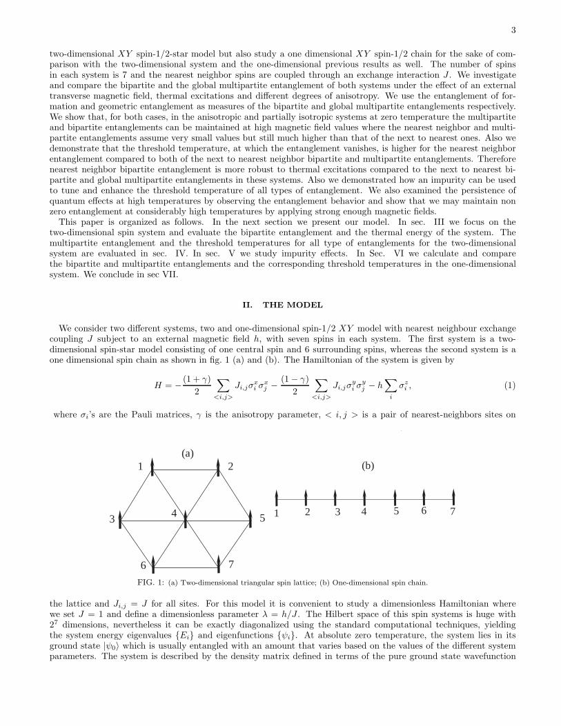
We consider two different systems, two and one-dimensional spin-1/2 XY model with nearest neighbour exchangecoupling J subject to an external magnetic field h, with seven spins in each system. The first system is a two-dimensional spin-star model consisting of one central spin and 6 surrounding spins, whereas the second system is aone dimensional spin chain as shown in fig. 1 (a) and (b). The Hamiltonian of the system is given by

H = − (1 + γ)

2

∑

<i,j>

Ji,jσxi σ

xj − (1− γ)

2

∑

<i,j>

Ji,jσyi σ

yj − h

∑

i

σzi , (1)

where σi’s are the Pauli matrices, γ is the anisotropy parameter, < i, j > is a pair of nearest-neighbors sites on

1 2

3 4 5

6 7

(a)

2 3 4 5 6 71

(b)

FIG. 1: (a) Two-dimensional triangular spin lattice; (b) One-dimensional spin chain.

the lattice and Ji,j = J for all sites. For this model it is convenient to study a dimensionless Hamiltonian wherewe set J = 1 and define a dimensionless parameter λ = h/J . The Hilbert space of this spin systems is huge with27 dimensions, nevertheless it can be exactly diagonalized using the standard computational techniques, yieldingthe system energy eigenvalues {Ei} and eigenfunctions {ψi}. At absolute zero temperature, the system lies in itsground state |ψ0〉 which is usually entangled with an amount that varies based on the values of the different systemparameters. The system is described by the density matrix defined in terms of the pure ground state wavefunction

4

|ψ0〉 as

ρ = |ψ0〉〈ψ0| . (2)

Now when the spin system is set into contact with a heat bath at an absolute temperature T , the system moves fromits initial pure state described by eq. (2) to a mixed thermal state, which is a mixture of the ground state and anumber Ne of excited states, represented by

ρT =1

Z{e−βE0|ψ0〉〈ψ0|+

Ne∑

i=1

e−βEi |ψi〉〈ψi|} , (3)

where β = 1/kT , k is Boltzmann constant and Z is the system partition function. The number of excited statesinvolved depends on temperature, where more states are added as the temperature is raised. This mixing of excitedstates with the ground state act as a destructive noise that reduces the amount of entanglement contained in thesystem. When the temperature reaches certain value, which varies based on the system characteristics and parametersvalues, the amount of noise created by the excites states due to thermal fluctuations is sufficient to turn the systeminto a disentangled state. This temperature is known as the threshold temperature, denoted by Tth , where below itthe system is guaranteed to be entangled [33].

III. THERMAL BIPARTITE ENTANGLEMENT IN TWO-DIMENSIONAL SPIN SYSTEM

To study the bipartite entanglement in the system, we confine our interest to the entanglement between only twospins, at any sites i and j [58]. All the information about the considered two sites i and j is contained in the reduceddensity matrix ρi,j which can be obtained from the entire system density matrix by integrating out all the spins statesexcept i and j. We adopt the entanglement of formation, as a well known measure of entanglement where Wootters[29] has shown that, for a pair of binary qubits, the concurrence C, which goes from 0 to 1, can be used to quantifyentanglement. The concurrence between two sites i and j is defined as

C(ρi,j) = max{0, ǫ1 − ǫ2 − ǫ3 − ǫ4}, (4)

where the ǫi’s are the eigenvalues of the Hermitian matrix R ≡√√

ρρ̃√ρ with ρ̃ = (σy ⊗ σy)ρ∗(σy ⊗ σy) and σy is

the Pauli matrix of the spin in y direction. For a pair of qubits the entanglement of formation is defined as,

E(ρi,j) = ǫ(C(ρi,j)), (5)

where ǫ is a function of C

ǫ(C) = h

(

1−√1− C2

2

)

, (6)

where h is the binary entropy function

h(x) = −x log2(x) − (1− x) log2(1− x). (7)

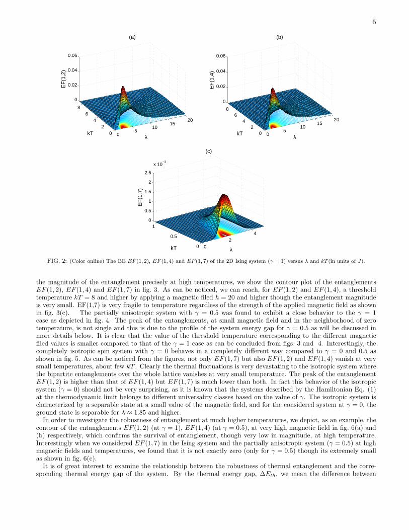
In our calculations we use the entanglement of formation EF as a measure of the bipartite entanglement. Usingthe mixed density matrix ρT defined in (3), one can evaluate the bipartite entanglement between any pair of spinsin the system. In this section we focus on studying the bipartite entanglement only in the two-dimensional spinsystem sketched in fig. 1(a). In fig. 2 we have explored the behaviour of the entanglements of the nearest neighborsEF (1, 2); EF (1, 4) and the next-to-next-to-nearest neighbor (nnnn) EF (1, 7) versus λ and the temperature KT forthe anisotropic Ising system (γ = 1). In fact the next-to-nearest neighbor (nnn) EF (1, 5) is very close to EF (1, 7),as we will show below, but EF (1, 7) shows sharper changes, which makes us focus on it. As can be noticed, thenearest neighbor bipartite entanglements between two border sites EF (1, 2) and between a border site and the centralone EF (1, 4) are strongest for very small magnetic field but very fragile away from the zero temperature. On theother hand, as the magnetic field is increased the entanglement maintains a small value which is more resistantto higher temperatures. Interestingly, the threshold temperature Tth at which the entanglement vanishes increasesmonotonically as the magnetic field increases. The (nnnn) entanglement EF(1,7) sustains only for very small valuesof magnetic field and in the vicinity of the zero temperature and its value is much smaller than the nearest neighborentanglements. In order to further investigate the thermal robustness of the entanglement state and determine

5

05

1015

20

02

46

8

0

0.02

0.04

0.06

λ

(a)

kT

EF

(1,2

)

05

1015

20

02

46

8

0

0.02

0.04

0.06

λ

(b)

kT

EF

(1,4

)

02

4

0

0.5

10

0.5

1

1.5

2

2.5

x 10−3

λ

(c)

kT

EF

(1,7

)

FIG. 2: (Color online) The BE EF (1, 2), EF (1, 4) and EF (1, 7) of the 2D Ising system (γ = 1) versus λ and kT (in units of J).

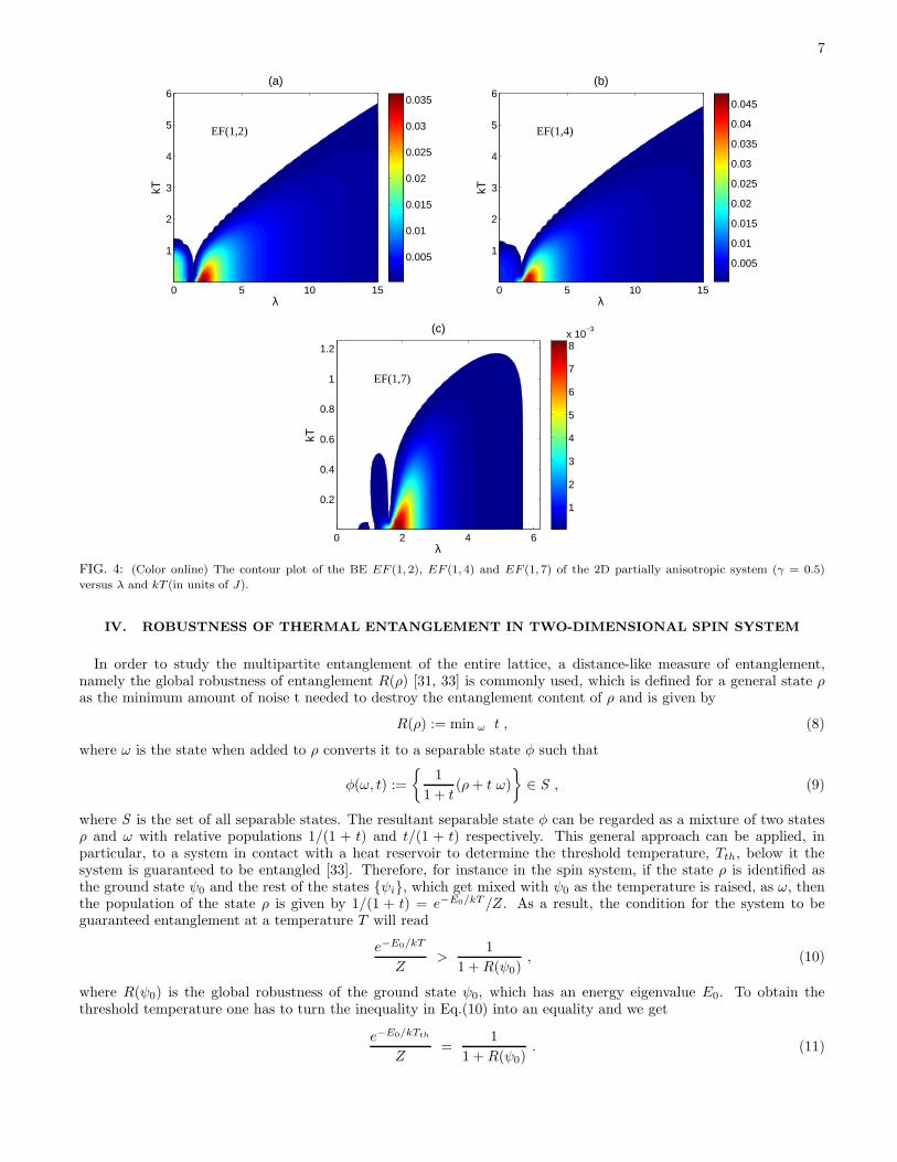
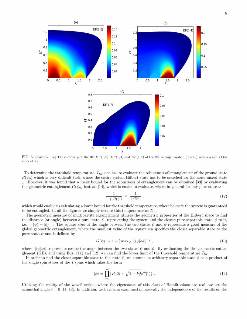
the magnitude of the entanglement precisely at high temperatures, we show the contour plot of the entanglementsEF (1, 2), EF (1, 4) and EF (1, 7) in fig. 3. As can be noticed, we can reach, for EF (1, 2) and EF (1, 4), a thresholdtemperature kT = 8 and higher by applying a magnetic filed h = 20 and higher though the entanglement magnitudeis very small. EF(1,7) is very fragile to temperature regardless of the strength of the applied magnetic field as shownin fig. 3(c). The partially anisotropic system with γ = 0.5 was found to exhibit a close behavior to the γ = 1case as depicted in fig. 4. The peak of the entanglements, at small magnetic field and in the neighborhood of zerotemperature, is not single and this is due to the profile of the system energy gap for γ = 0.5 as will be discussed inmore details below. It is clear that the value of the threshold temperature corresponding to the different magneticfiled values is smaller compared to that of the γ = 1 case as can be concluded from figs. 3 and 4. Interestingly, thecompletely isotropic spin system with γ = 0 behaves in a completely different way compared to γ = 0 and 0.5 asshown in fig. 5. As can be noticed from the figures, not only EF (1, 7) but also EF (1, 2) and EF (1, 4) vanish at verysmall temperatures, about few kT . Clearly the thermal fluctuations is very devastating to the isotropic system wherethe bipartite entanglements over the whole lattice vanishes at very small temperature. The peak of the entanglementEF (1, 2) is higher than that of EF (1, 4) but EF (1, 7) is much lower than both. In fact this behavior of the isotropicsystem (γ = 0) should not be very surprising, as it is known that the systems described by the Hamiltonian Eq. (1)at the thermodynamic limit belongs to different universality classes based on the value of γ. The isotropic system ischaracterized by a separable state at a small value of the magnetic field, and for the considered system at γ = 0, theground state is separable for λ ≈ 1.85 and higher.In order to investigate the robustness of entanglement at much higher temperatures, we depict, as an example, the

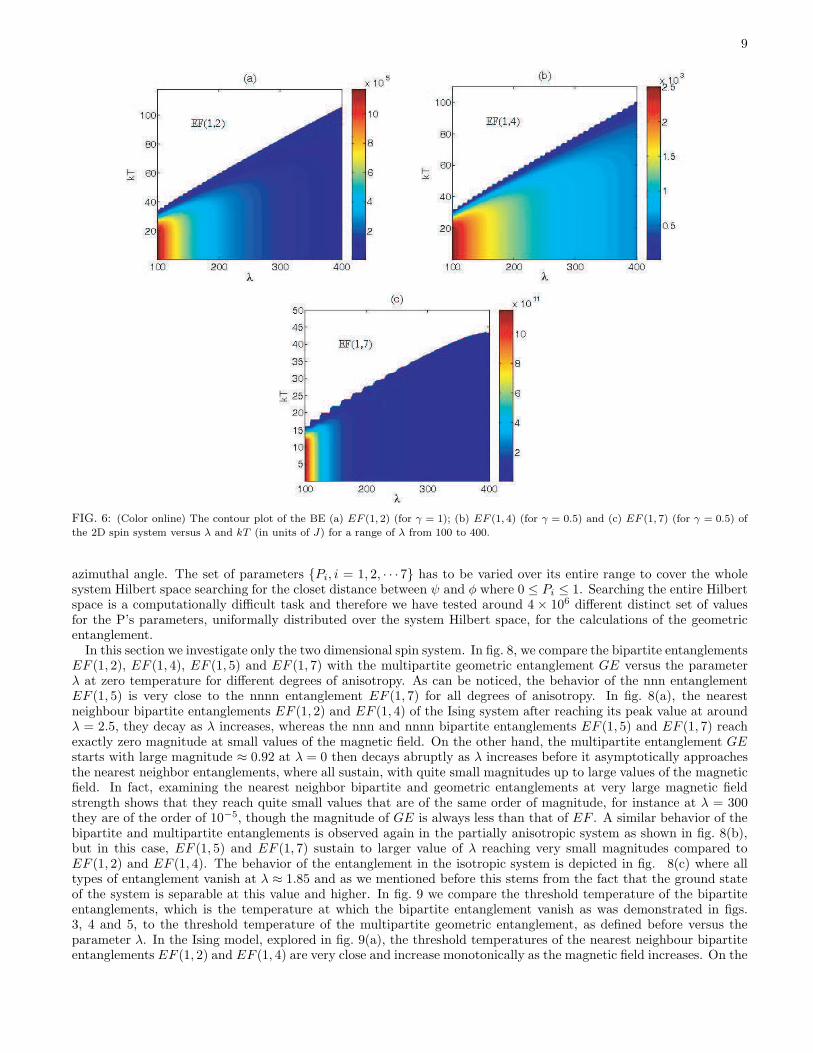
contour of the entanglements EF (1, 2) (at γ = 1), EF (1, 4) (at γ = 0.5), at very high magnetic field in fig. 6(a) and(b) respectively, which confirms the survival of entanglement, though very low in magnitude, at high temperature.Interestingly when we considered EF (1, 7) in the Ising system and the partially anisotropic system (γ = 0.5) at highmagnetic fields and temperatures, we found that it is not exactly zero (only for γ = 0.5) though its extremely smallas shown in fig. 6(c).It is of great interest to examine the relationship between the robustness of thermal entanglement and the corre-

sponding thermal energy gap of the system. By the thermal energy gap, ∆Eth, we mean the difference between

6

(a)

λ

kT

0 5 10 15 20

1

2

3

4

5

6

7

8

0.01

0.02

0.03

0.04

0.05

EF(1,2)

(b)

λ

kT

0 5 10 15 20

1

2

3

4

5

6

7

8

0.01

0.02

0.03

0.04

0.05

EF(1,4)

(c)

λ

kT

0 1 2 3 4 5

0.2

0.4

0.6

0.8

1

0.5

1

1.5

2

x 10−3

EF(1,7)

FIG. 3: (Color online) The contour plot of the BE EF (1, 2), EF (1, 4) and EF (1, 7) of the 2D Ising system (γ = 1) versus λ and kT (in

units of J).

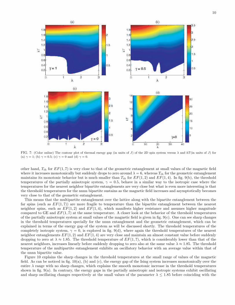
the mean (ensemble average) energy of the system at temperature T and the system ground state energy, i.e.∆Eth = 〈E〉 − E0.In fig. 7 (a), (b), and (c) we present the contour plots of energy gap for the systems with γ = 1, 0.5 and 0 respectively

versus λ and kT for small values of λ. As can be seen, there is a clear differences between the different cases, wherethe energy gap in the Ising system shows one sharp minimum before increasing montonically as λ increases whichgives raise to one corresponding sharp peak of entanglement in that case at the small values of λ. The energy gaps inthe partially anisotropic and isotropic systems show two and multiple minima respectively before they also increasemontonically with λ, which causes the double peaks and multiple peaks, with different relative intensities, in the twosystems respectively. This explains the different profiles of the entanglement peaks, at small values of the magneticfield, as the degree of anisotropy changes as demonstrated in figs. 3, 4 and 5. On the other hand, the thermal energygap at the different anisotropic values looks asymptotically (at high magnetic field) the same, as shown in fig. 7(d)for the case γ = 0 for instance.Remarkably, one can see a strong correspondence between the strength and survival of entanglement, particularly

for γ = 0.5 and 1 and the value of the energy gap when comparing figs. 3, 4 and 7. The energy gap is either zero(the white regions of the contour plot) or quit small in the domains of non-zero entanglement. As can be noticedthe thermal energy gap increases monotonically as the magnetic field intensity increases which explains the survivalof the entanglement, despite its small magnitude, at relatively high temperatures and its strong resistance againstthermal excitations compared to the high magnitude entanglement at the small values of the magnetic field which isvery fragile to temperature. It is important to emphasis here that though the energy gap profile looks asymptoticallyalmost the same for the three anisotropic parameter values, nevertheless the entanglement in the isotropic system(γ = 0) in contrary to the other two cases vanishes at very low temperature regardless of the energy gap value andthis is due to the fact that this system ground state, as we mentioned before, is disentangled for λ ≈ 1.85 and higher.

7

(a)

λ

kT

0 5 10 15

1

2

3

4

5

6

0.005

0.01

0.015

0.02

0.025

0.03

0.035

EF(1,2)

(b)

λ

kT

0 5 10 15

1

2

3

4

5

6

0.005

0.01

0.015

0.02

0.025

0.03

0.035

0.04

0.045

EF(1,4)

(c)

λ

kT

0 2 4 6

0.2

0.4

0.6

0.8

1

1.2

1

2

3

4

5

6

7

8x 10

−3

EF(1,7)

FIG. 4: (Color online) The contour plot of the BE EF (1, 2), EF (1, 4) and EF (1, 7) of the 2D partially anisotropic system (γ = 0.5)

versus λ and kT (in units of J).

IV. ROBUSTNESS OF THERMAL ENTANGLEMENT IN TWO-DIMENSIONAL SPIN SYSTEM

In order to study the multipartite entanglement of the entire lattice, a distance-like measure of entanglement,namely the global robustness of entanglement R(ρ) [31, 33] is commonly used, which is defined for a general state ρas the minimum amount of noise t needed to destroy the entanglement content of ρ and is given by

R(ρ) := min ω t , (8)

where ω is the state when added to ρ converts it to a separable state φ such that

φ(ω, t) :=

{

1

1 + t(ρ+ t ω)

}

∈ S , (9)

where S is the set of all separable states. The resultant separable state φ can be regarded as a mixture of two statesρ and ω with relative populations 1/(1 + t) and t/(1 + t) respectively. This general approach can be applied, inparticular, to a system in contact with a heat reservoir to determine the threshold temperature, Tth, below it thesystem is guaranteed to be entangled [33]. Therefore, for instance in the spin system, if the state ρ is identified asthe ground state ψ0 and the rest of the states {ψi}, which get mixed with ψ0 as the temperature is raised, as ω, thenthe population of the state ρ is given by 1/(1 + t) = e−E0/kT /Z. As a result, the condition for the system to beguaranteed entanglement at a temperature T will read

e−E0/kT

Z>

1

1 +R(ψ0), (10)

where R(ψ0) is the global robustness of the ground state ψ0, which has an energy eigenvalue E0. To obtain thethreshold temperature one has to turn the inequality in Eq.(10) into an equality and we get

e−E0/kTth

Z=

1

1 +R(ψ0). (11)

8

(a)

λ

kT

0 0.5 1 1.5 2 2.5

0.2

0.4

0.6

0.8

1

1.2

0.02

0.04

0.06

0.08

0.1

0.12

0.14EF(1,2)

(b)

λ

kT

0 0.5 1 1.5 2 2.5

0.2

0.4

0.6

0.8

1

1.2

0.05

0.1

0.15

0.2EF(1,4)

(c)

λ

kT

0 0.5 1 1.5 2

0.1

0.2

0.3

0.4

0.5

0.6

0.7

0.8

0.02

0.04

0.06

0.08

0.1

EF(1,7)

FIG. 5: (Color online) The contour plot the BE EF (1, 2), EF (1, 4) and EF (1, 7) of the 2D isotropic system (γ = 0.) versus λ and kT (in

units of J).

To determine the threshold temperature, Tth, one has to evaluate the robustness of entanglement of the ground stateR(ψ0) which is very difficult task, where the entire system Hilbert state has to be searched for the noise mixed stateω. However, it was found that a lower bound for the robustness of entanglement can be obtained [33] by evaluatingthe geometric entanglement G(ψ0) instead [14], which is easier to evaluate, where in general for any pure state ψ

1

1 +R(ψ)≤ 1

2 G(ψ), (12)

which would enable us calculating a lower bound for the threshold temperature, where below it the system is guaranteedto be entangled. In all the figures we simply denote this temperature as Tth.The geometric measure of multipartite entanglement utilizes the geometric properties of the Hilbert space to find

the distance (or angle) between a pure state, ψ, representing the system and the closest pure separable state, φ to it,i.e. || |ψ〉 − |φ〉 ||. The square sine of the angle between the two states ψ and φ represents a good measure of theglobal geometric entanglement, where the smallest value of the square sin specifies the closet separable state to thepure state ψ and is defined by

G(ψ) := 1− [ max φ ||〈ψ|φ〉|| ]2 , (13)

where ||〈ψ|φ〉|| represents cosine the angle between the two states ψ and φ. By evaluating the the geometric entan-glement (GE), and using Eqs. (11) and (12) we can find the lower limit of the threshold temperature Tth.In order to find the closet separable state to the state ψ, we assume an arbitrary separable state φ as a product of

the single spin states of the 7 spins which takes the form

|φ〉 =i=7∏

i=1

{Pi|0〉+√

1− P 2i e

iδ|1〉} . (14)

Utilizing the reality of the wavefunction, where the eigenstates of this class of Hamiltonians are real, we set theazimuthal angle δ = 0 [14, 18]. In addition, we have also examined numerically the independence of the results on the

9

FIG. 6: (Color online) The contour plot of the BE (a) EF (1, 2) (for γ = 1); (b) EF (1, 4) (for γ = 0.5) and (c) EF (1, 7) (for γ = 0.5) of

the 2D spin system versus λ and kT (in units of J) for a range of λ from 100 to 400.

azimuthal angle. The set of parameters {Pi, i = 1, 2, · · · 7} has to be varied over its entire range to cover the wholesystem Hilbert space searching for the closet distance between ψ and φ where 0 ≤ Pi ≤ 1. Searching the entire Hilbertspace is a computationally difficult task and therefore we have tested around 4 × 106 different distinct set of valuesfor the P’s parameters, uniformally distributed over the system Hilbert space, for the calculations of the geometricentanglement.In this section we investigate only the two dimensional spin system. In fig. 8, we compare the bipartite entanglements

EF (1, 2), EF (1, 4), EF (1, 5) and EF (1, 7) with the multipartite geometric entanglement GE versus the parameterλ at zero temperature for different degrees of anisotropy. As can be noticed, the behavior of the nnn entanglementEF (1, 5) is very close to the nnnn entanglement EF (1, 7) for all degrees of anisotropy. In fig. 8(a), the nearestneighbour bipartite entanglements EF (1, 2) and EF (1, 4) of the Ising system after reaching its peak value at aroundλ = 2.5, they decay as λ increases, whereas the nnn and nnnn bipartite entanglements EF (1, 5) and EF (1, 7) reachexactly zero magnitude at small values of the magnetic field. On the other hand, the multipartite entanglement GEstarts with large magnitude ≈ 0.92 at λ = 0 then decays abruptly as λ increases before it asymptotically approachesthe nearest neighbor entanglements, where all sustain, with quite small magnitudes up to large values of the magneticfield. In fact, examining the nearest neighbor bipartite and geometric entanglements at very large magnetic fieldstrength shows that they reach quite small values that are of the same order of magnitude, for instance at λ = 300they are of the order of 10−5, though the magnitude of GE is always less than that of EF . A similar behavior of thebipartite and multipartite entanglements is observed again in the partially anisotropic system as shown in fig. 8(b),but in this case, EF (1, 5) and EF (1, 7) sustain to larger value of λ reaching very small magnitudes compared toEF (1, 2) and EF (1, 4). The behavior of the entanglement in the isotropic system is depicted in fig. 8(c) where alltypes of entanglement vanish at λ ≈ 1.85 and as we mentioned before this stems from the fact that the ground stateof the system is separable at this value and higher. In fig. 9 we compare the threshold temperature of the bipartiteentanglements, which is the temperature at which the bipartite entanglement vanish as was demonstrated in figs.3, 4 and 5, to the threshold temperature of the multipartite geometric entanglement, as defined before versus theparameter λ. In the Ising model, explored in fig. 9(a), the threshold temperatures of the nearest neighbour bipartiteentanglements EF (1, 2) and EF (1, 4) are very close and increase monotonically as the magnetic field increases. On the

10

FIG. 7: (Color online) The contour plot of thermal energy gap (in units of J) of the 2D spin system versus λ and kT (in units of J) for

(a) γ = 1; (b) γ = 0.5; (c) γ = 0 and (d) γ = 0.

other hand, Tth for EF (1, 7) is very close to that of the geometric entanglement at small values of the magnetic fieldwhere it increases monotonically but suddenly drops to zero around λ = 6, whereas Tth for the geometric entanglementmaintains its monotonic behavior but is much smaller than Tth for EF (1, 2) and EF (1, 4). In fig. 9(b), the thresholdtemperatures of the partially anisotropic system, γ = 0.5, behave in a similar way to the isotropic case where thetemperatures for the nearest neighbor bipartite entanglements are very close but what is even more interesting is thatthe threshold temperatures for the nnnn bipartite sustains as the magnetic field increases and asymptotically becomesvery close to that of the geometric entanglement.This means that the multipartite entanglement over the lattice along with the bipartite entanglement between the

far spins (such as EF (1, 7)) are more fragile to temperature than the bipartite entanglement between the nearestneighbor spins, such as EF (1, 2) and EF (1, 4), which manifests higher resistance and assumes higher magnitudecompared to GE and EF (1, 7) at the same temperature. A closer look at the behavior of the threshold temperaturesof the partially anisotropic system at small values of the magnetic field is given in fig. 9(c). One can see sharp changesin the threshold temperatures specially for the nnnn entanglement and the geometric entanglement, which can beexplained in terms of the energy gap of the system as will be discussed shortly. The threshold temperatures of thecompletely isotropic system, γ = 0, is explored in fig. 9(d), where again the threshold temperatures of the nearestneighbor entanglements EF (1, 2) and EF (1, 4) are very close and maintain an almost constant value before suddenlydropping to zero at λ ≈ 1.85. The threshold temperature of EF (1, 7), which is considerably lower than that of thenearest neighbors, increases linearly before suddenly dropping to zero also at the same value λ ≈ 1.85. The thresholdtemperature of the multipartite entanglement exhibits an oscillatory behavior with an average value within that ofthe nnnn bipartite value.Figure 10 explains the sharp changes in the threshold temperatures at the small range of values of the magnetic

field. As can be noticed in fig. 10(a), (b) and (c), the energy gap of the Ising system increases monotonically over theentire λ range with no sharp changes, which explains the smooth monotonic increase in the threshold temperaturesshown in fig. 9(a). In contrary, the energy gaps in the partially anisotropic and isotropic systems exhibit oscillatingand sharp oscillating changes respectively at the small values of the parameter λ ≤ 1.85 before coinciding with the

11

0 5 10 15 200

0.01

0.02

0.03

0.04

0.05

0.06(a)

λ

E

GEEF(1,7)EF(1,5)EF(1,4)EF(1,2)

γ = 1

0 5 10 15 200

0.01

0.02

0.03

0.04

0.05

0.06(b)

λ

E

γ = 0.5

0 0.5 1 1.5 20

0.2

0.4

0.6

0.8

1(c)

λ

E

γ = 0

FIG. 8: (Color online) The entanglements EF (1, 2), EF (1, 4), EF (1, 5), EF (1, 7) and geometric entanglement of the 2D spin system

versus λ for γ = 0, 0.5 and 1 at zero temperature. The legends are as shown in subfigure (a).

anisotropic curve and increasing monotonically as shown in fig. 10. Interestingly, by comparing the behavior of thethreshold temperatures, particularly of the multipartite entanglement, in fig. 9 to that of the energy gaps in fig. 10 onecan notice the strict correspondence between them; the minima (and maxima) in the threshold temperatures coincidewith that of the energy gaps on the parameter λ scale and when the energy gap increases monotonically, the thresholdtemperature follows that behavior too. The impact of the energy gap on the multipartite entanglement is strongercompared to the bipartite entanglement due to the fact that the energy gap is calculated for the entire (multipartite)system. The effect of the number of distinctive set of parameters {Pi, i = 1, 2, · · ·7} on the accuracy of the resultsis examined in fig. 11 where two different numbers, 2 × 105 and 4 × 106 are compared in plotting the multipartiteentanglement for γ = 1 and the threshold temperature for γ = 0.5 , which shows a very strong coincidence.

V. IMPURITY EFFECT

The imperfection and disorder in real physical systems have been always a big concern when studying the differentquantum properties of many body systems [21, 50]. Disorder and lack of homogeneity and isotropy cause a breakof the translational symmetry and consequently the scaling of the entropy and all related quantities. An essentialsource of disorder is the presence of impurities in the physical system. The effect of quantum impurities in many bodysystems and the quantification of the entanglement in these systems have been investigated [50]. The Von Neumannentropy was used to quantify the single site impurity entanglement in the considered systems. At finite temperature,the thermodynamic impurity entropy is used to quantify entanglement especially in Kondo impurity systems [51, 52].It was shown that the entanglement is significantly affected by the presence of the impurity even in absence of physicalcoupling to the impurity itself. In a previous work, it was demonstrated that the entanglement and ergodicity in twodimensional spin system can be tuned using impurities and anisotropy [53]. The effect of impurities on the spinrelaxation rate [54] and dynamics of entanglement in one-dimensional spin systems have been investigated [55]. Thedecay rate of the spin oscillation was found to be significantly affected by the coupling strength of the impurity spin.

12

0 5 10 15 200

2

4

6

8

10(a)

λ

Tth

(1,2)(1,4)(1,7)GE

γ = 1

0 5 10 15 200

2

4

6

8

10(b)

λ

Tth

γ = 0.5

0 0.5 1 1.5 2 2.5 30

0.2

0.4

0.6

0.8

1

1.2

1.4

1.6

(c)

λ

Tth

γ = 0.5

0 0.5 1 1.5 20

0.2

0.4

0.6

0.8

1

1.2

1.4(d)

λ

Tth

γ = 0

FIG. 9: (Color online) The threshold temperatures (in units of J) corresponding to the entanglements EF(1,2), EF(1,4), EF(1,7) and

geometric entanglement of the 2D spin system versus λ for γ = 0, 0.5 and 1. The legends are as shown in subfigure (a).

In this section we study the effect of a single impurity located at the central site on the threshold temperatureof the different types of entanglement in the lattice. The single impurity is a spin that is coupled to its nearestneighbors through an exchange interaction J ′ which differs from that between the other sites. We set J ′ = (α + 1)Jwhere α is the impurity strength parameter. Here we consider 3 different cases for the impurity strength, α = −0.5, 0and 0.5 representing weak, null and strong ones respectively. In fact, such a system of 7-spins with the central spinhaving a different coupling strength from the surrounding ones can be realized, for instance, in a system of coupledsemiconductor quantum dots where the coupling between the valence electrons on the different dots is the exchangeinteraction which can be controlled by raising or lowering the potential barrier between the dots [56].In figs. 12(a), (b) and (c) we study the effect of the central impurity, with different strengths, in the two-dimensional

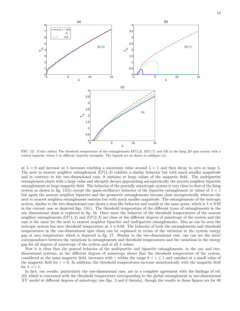
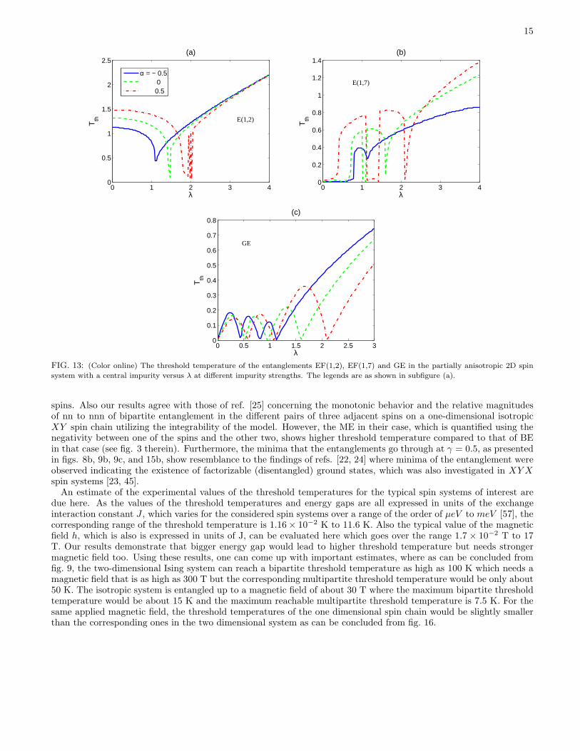
Ising lattice on the nn bipartite EF (1, 2), nnnn bipartite EF (1, 7) and multipartite entanglement GE respectively.As can be noticed, the impurity strength has minor effect on EF (1, 2) where almost no change can be observed. Inter-estingly, in the case of EF (1, 7), the critical value of the magnetic field at which the entanglement vanishes increasesas the impurity strength increases. For strong impurity case, EF (1, 7) never vanish and increases montonically asλ increases. This means that the impurity can be used to significantly preserve and enhance nnnn entanglement athigh temperature and magnetic field in the Ising system, which is also the case for GE as can be noticed in fig. 12(c).The partially anisotropic system is explored in fig. 13. The impurity has a significant effect on EF (1, 2) only at smallvalues of λ, where it shifts the threshold minimum towards the right and creates an oscillation for strong impurityvalue. The asymptotic value of EF (1, 2) at large λ is not affected by the impurity strength. On the other hand, whilethe impurity strength enhances the nnnn asymptotic entanglement, it reduces the global entanglement but shifts theminima of Tth towards higher magnetic field values. The effect of the impurity on the isotropic system, with γ = 0,is shown in fig. 14, where increseing the impurity strength clearly enhances all types of entanglement. In addition, italso shift the magnetic field critical value at which all entanglements vanish toward higher values. In fact, our resultsconcerning the threshold temperatures here confirm the findings in a previous work [53] where it was shown that theentanglement can be enhanced or quenched in the spin system depending on the degree of anisotropy and the strengthof the impurities.

13

0 0.5 1 1.50

0.02

0.04

0.06

0.08

0.1(a)

λ

∆ E

γ=0.5γ=1

0 0.5 1 1.5 20

0.1

0.2

0.3

0.4

0.5

0.6

0.7

0.8

(b)

λ

∆ E

γ=0

0 1 2 3 4 50

1

2

3

4

5

6(c)

λ

∆ E

γ=0γ=0.5γ=1

FIG. 10: (Color online) The energy gap (in units of J) of the 2D spin system versus λ for γ = 0, 0.5 and 1.

0 2 4 6 8 100

0.2

0.4

0.6

0.8

1(a)

λ

E

n= 4× 106

n= 2× 105

γ=1

0 0.5 1 1.5 2 2.50

0.1

0.2

0.3

0.4

0.5

0.6

0.7(b)

λ

Tth

n= 4× 106

n= 2× 105

γ = 0

FIG. 11: (Color online) (a) The geometric entanglement of the 2D Ising system (γ = 1) and (b) the threshold temperature (in units of

J) of the 2D isotropic system (γ = 0), for two different numbers of the set of parameters {Pi}, n = 2× 105 and 4× 106.

VI. ENTANGLEMENTS AND THRESHOLD TEMPERATURES IN ONE DIMENSIONAL SPIN

SYSTEM

Now let us consider a one dimensional XY spin chain consisting of 7 spins, as sketched in fig. 1(b), which isdescribed by the same Hamiltonian Eq. (1) where in this case the exchange interaction Ji,j exists only between eachspin and its two nearest neighbor spins on the chain. The system shows a close behavior to what we have seen in thetwo-dimensional case.In fig. 15(a) we compare the bipartite entanglements to the multipartite entanglement for the Ising system, where as

can be seen the nearest neighbor entanglements EF (1, 2) and EF (2, 3) are very close as they start with zero magnitude

14

0 5 10 150

1

2

3

4

5

6

7

8(a)

λ

Tth

α = − 0.5 0 0.5

E(1,2)

0 5 10 150

0.5

1

1.5

2

2.5

3

3.5

4(b)

λ

Tth

E(1,7)

0 5 10 150

0.5

1

1.5

2

2.5

3

3.5

4(c)

λ

Tth

GE

FIG. 12: (Color online) The threshold temperature of the entanglements EF(1,2), EF(1,7) and GE in the Ising 2D spin system with a

central impurity versus λ at different impurity strengths. The legends are as shown in subfigure (a).

at λ = 0 and increase as λ increases reaching a maximum value around λ = 1 and then decay to zero at large λ.The next to nearest neighbor entanglement EF (1, 3) exhibits a similar behavior but with much smaller magnitudeand in contrary to the two-dimensional case, it sustains at large values of the magnetic field. The multipartiteentanglement starts with a large value and abruptly decays approaching asymptotically the nearest neighbor bipartiteentanglements at large magnetic field. The behavior of the partially anisotropic system is very close to that of the Isingsystem as shown in fig. 15(b) except the quasi-oscillatory behavior of the bipartite entanglement at values of λ < 1but again the nearest neighbor bipartite and the geometric entanglements become close asymptotically whereas thenext to nearest neighbor entanglement sustains but with much smaller magnitude. The entanglements of the isotropicsystem, similar to the two-dimensional case shows a step-like behavior and vanish at the same point, which is λ ≈ 0.92in the current case as depicted figs. 15(c). The threshold temperature of the different types of entanglements in theone dimensional chain is explored in fig. 16. Once more the behavior of the threshold temperatures of the nearestneighbor entanglements EF (1, 2) and EF (2, 3) are close at the different degrees of anisotropy of the system and thecase is the same for the next to nearest neighbor bipartite and multipartite entanglements. Also as can be seen theisotropic system has zero threshold temperature at λ ≈ 0.92. The behavior of both the entanglements and thresholdtemperatures in the one-dimensional spin chain can be explained in terms of the variation in the system energygap at zero temperature which is depicted in fig. 17. Similar to the two-dimensional case, one can see the strictcorrespondence between the variations in entanglements and threshold temperatures and the variations in the energygap for all degrees of anisotropy of the system and at all λ values.Now it is clear that the general behavior of the multipartite and bipartite entanglements, in the one and two-

dimensional systems, at the different degrees of anisotropy shows that the threshold temperature of the system,considered at the same magnetic field, increases with γ within the range 0 < γ ≤ 1 and vanishes at a small value ofthe magnetic field for γ = 0. In addition, the threshold temperatures increase monotonically with the magnetic fieldfor λ >> 1.In fact, our results, particularly the one-dimensional case, are in a complete agreement with the findings of ref.

[35] which is concerned with the threshold temperature corresponding to the global entanglement in one-dimensionalXY model at different degrees of anisotropy (see figs. 5 and 6 therein), though the results in those figures are for 80

15

0 1 2 3 40

0.5

1

1.5

2

2.5(a)

λ

Tth

α = − 0.5 0 0.5

E(1,2)

0 1 2 3 40

0.2

0.4

0.6

0.8

1

1.2

1.4(b)

λ

Tth

E(1,7)

0 0.5 1 1.5 2 2.5 30

0.1

0.2

0.3

0.4

0.5

0.6

0.7

0.8(c)

λ

Tth

GE

FIG. 13: (Color online) The threshold temperature of the entanglements EF(1,2), EF(1,7) and GE in the partially anisotropic 2D spin

system with a central impurity versus λ at different impurity strengths. The legends are as shown in subfigure (a).

spins. Also our results agree with those of ref. [25] concerning the monotonic behavior and the relative magnitudesof nn to nnn of bipartite entanglement in the different pairs of three adjacent spins on a one-dimensional isotropicXY spin chain utilizing the integrability of the model. However, the ME in their case, which is quantified using thenegativity between one of the spins and the other two, shows higher threshold temperature compared to that of BEin that case (see fig. 3 therein). Furthermore, the minima that the entanglements go through at γ = 0.5, as presentedin figs. 8b, 9b, 9c, and 15b, show resemblance to the findings of refs. [22, 24] where minima of the entanglement wereobserved indicating the existence of factorizable (disentangled) ground states, which was also investigated in XYXspin systems [23, 45].An estimate of the experimental values of the threshold temperatures for the typical spin systems of interest are

due here. As the values of the threshold temperatures and energy gaps are all expressed in units of the exchangeinteraction constant J , which varies for the considered spin systems over a range of the order of µeV to meV [57], thecorresponding range of the threshold temperature is 1.16× 10−2 K to 11.6 K. Also the typical value of the magneticfield h, which is also is expressed in units of J, can be evaluated here which goes over the range 1.7 × 10−2 T to 17T. Our results demonstrate that bigger energy gap would lead to higher threshold temperature but needs strongermagnetic field too. Using these results, one can come up with important estimates, where as can be concluded fromfig. 9, the two-dimensional Ising system can reach a bipartite threshold temperature as high as 100 K which needs amagnetic field that is as high as 300 T but the corresponding multipartite threshold temperature would be only about50 K. The isotropic system is entangled up to a magnetic field of about 30 T where the maximum bipartite thresholdtemperature would be about 15 K and the maximum reachable multipartite threshold temperature is 7.5 K. For thesame applied magnetic field, the threshold temperatures of the one dimensional spin chain would be slightly smallerthan the corresponding ones in the two dimensional system as can be concluded from fig. 16.

16

0 1 2 3 40

0.2

0.4

0.6

0.8

1

1.2

1.4

1.6(a)

λ

Tth

−0.500.5

E(1,2)

0 0.5 1 1.5 2 2.5 30

0.2

0.4

0.6

0.8

1

1.2

1.4(b)

λ

Tth

E(1,7)

0 0.5 1 1.5 2 2.5 30

0.1

0.2

0.3

0.4

0.5

0.6

0.7

0.8(c)

λ

Tth

GE

FIG. 14: (Color online) The threshold temperature of the entanglements EF(1,2), EF(1,7) and GE in the isotropic 2D spin system with

a central impurity versus λ at different impurity strengths. The legends are as shown in subfigure (a).

VII. QUANTUM PHASE SPACE OF XY SPIN SYSTEMS

Quantum phase transition in a many-body system happens either when an actual crossing takes place betweenthe excited state and the ground state or a limiting avoided level crossing between them exists, i.e., an energy gapbetween the two states that vanishes in the infinite system size limit at the critical point [16]. When a many-bodysystem crosses a critical point, significant changes in both its wave function and ground-state energy take place, whichcan be realized in the behavior of the entanglement function and its derivatives [53, 58, 59]. It is well known that aninfinite many body system (i.e. at the thermodynamic limit) exhibits clear singularity at the critical point. However,finite size systems may still show strong tendency for being singular closer to the actual critical point of the system,which improves with the system size [53, 59].The Hamiltonian Eq.(1) describes a family of models with different distinct phases at the thermodynamic limit

(N → ∞). The quantum phase diagram for the one-dimensional system, in terms of γ and h, is well determined andcontains three different phases: Oscillatory, ferromagnetic and paramagnetic [60]. At the thermodynamic limit, thesystem reaches the isotropic and Ising limits at γ = 1 and 0 respectively. The system belongs to a universality class,the istropic (XX), at γ = 0 whereas it belongs to a different class, Ising (aniostropic XY ), in the range 0 < γ ≤ 1.The system possesses a quantum critical point at λ = λc = 1, where this point dictates the transition between differentphases of the system depending on the value of γ. The system at all degrees of anisotropy exists in the paramagneticphase for λ > λc. For γ2 + λ2 < λ2c and γ 6= 0 the system exits in the oscillatory phase whereas for γ2 + λ2 > λ2cand λ < 1 is paramagnetic. The phase diagram of the infinite two-dimensional system, though is very similar tothe one-dimensional case, is not well established due to the lack of analytic solution, computational difficulty andthe different structures that the system may have. Many efforts have been directed to the prediction of the criticalvalue of λc in the two dimensional spin system. For instance, the Renormalization group method has been appliedto the two dimensional infinite triangular (square) lattice and estimated a critical point at λc = 4.75784(2.62975)[61], whereas the finite size scaling method applied to the square lattice predicts λc = 3.044 [62]. The point (withtendency to singularity) in the finite two-dimensional spin system with 7-sites considered in this paper (and also for19-sites) was estimated previously and found to be λc = 1.64 and 3.01 for the 7-sites and 19-sites systems respectively

17

0 5 10 15 200

0.05

0.1

0.15

0.2

0.25(a)

λ

E

GEEF(1,2)EF(2,3)EF(1,3)γ = 1

0 2 4 6 80

0.05

0.1

0.15

0.2

0.25(b)

λ

E

γ = 0.5

0 0.2 0.4 0.6 0.8 10

0.1

0.2

0.3

0.4

0.5

0.6

0.7

0.8

(C)

λ

E

FIG. 15: (Color online) The entanglements EF(1,2), EF(2,3), EF(1,3) and geometric entanglement of the 1D spin system versus λ for

γ = 0, 0.5 and 1 at zero temperature. The legends are as shown in subfigure (a).

52.

by studying the pairwise concurrence and its derivative in the system [59].Though we emphasis here that the quantum phase transitions can take place only in the infinite system size

(in the thermodynamic limit) we will try to draw a relation here between the behavior of the entanglements andthe threshold temperatures in our considered systems and the different phases of the system. As one can noticefor the Ising system (γ = 1) the bipartite entanglements have one single peak, where in fact its derivative locatesthe point of strong tendency for being singular [53, 59] before decaying montonically with λ and the geometricentanglement decays montonically from large value. This behavior is reflected also in the threshold temperatures,which increase montonically with λ. This profile of the entanglements and temperatures can be related to transitionfrom ferromagnetic to paramagnetic states for the Ising system as λ increases crossing the expected critical point. Inthe partially anisotropic system γ = 0.5, the entanglements (threshold temperatures) exhibit few maxima and minimawith λ before montonically decreasing (increasing) which can be explained in terms of the transition of the systemfrom oscillatory to ferromagnetic and finally to the paramagnetic phase at the critical point. Finally the isotropicsystem shows sharp changes in the entanglements (threshold temperatures)as they decay before vanishing at λ ≈ 1.85,which can be explained in terms of transition from the oscillatory phase to paramagnetic phase and as we mentionedbefore the vanishing of all entanglements and threshold temperatures is due to the fact that the isotropic system hasa disentangled state for any magnetic field higher than this critical point.

VIII. CONCLUSIONS

We have investigated the robustness of bipartite and multipartite entanglement in one and two-dimensional XYspin-1/2 lattices in an external magnetic field h against thermal excitations. The spins are coupled to each otherthrough nearest neighbor exchange interaction J . The number of spins in the lattice is 7, which are coupled to aheat bath at temperature T . We have compared the bipartite entanglement to the multipartite entanglement versusthe external applied magnetic field and temperature. Also we compared the threshold temperature at which the

18

0 5 10 15 200

2

4

6

8

10(a)

λ

Tth

(1,2)(2,3)(1,3)GE

γ = 1

0 5 10 15 200

2

4

6

8

10(b)

λ

Tth

γ = 0.5

0 0.5 1 1.5 2 2.5 30

0.2

0.4

0.6

0.8

1

1.2

1.4

1.6

(c)

λ

Tth

γ = 0.5

0 0.2 0.4 0.6 0.8 10

0.2

0.4

0.6

0.8

1

1.2(d)

λ

Tth

γ = 0

FIG. 16: (Color online) The threshold temperatures (in units of J) corresponding to the entanglements EF(1,2), EF(2,3), EF(1,3) and

geometric entanglement of the 1D spin system versus λ for γ = 0, 0.5 and 1. The legends are as shown in subfigure (a).

entanglement vanishes in both cases. We used the entanglement as a measure of the bipartite entanglement and thegeometric measure to evaluate the multipartite entanglement of the system.In the one and two-dimensional cases for the anisotropic and partially anisotropic spin systems at zero temperature,

the nearest neighbor bipartite and multipartite entanglement can be maintained at large magnetic fields, though wouldhave very small values, which are still much higher than that of the next to nearest neighbor entanglements exceptin the two-dimensional Ising system where the latter vanishes at small value of the field. In the isotropic systemcase, all types of entanglement vanish at the same small value of the magnetic field. The nearest neighbor bipartitethreshold temperature was found to be higher than that of the next to nearest neighbor bipartite and multipartitewhere the temperatures of the last two get closer asymptotically and the three of them increase monotonically as themagnetic field increases. The exception is the threshold temperature of the nearest neighbor entanglement in the two-dimensional Ising system which vanishes as small value of the magnetic field. Accordingly the bipartite entanglementof the far spins of the system and the multipartite entanglement are less resilient toward thermal excitations comparedto the nearest neighbour entanglement. All the threshold temperatures of the isotropic system vanish exactly at thesame value of the magnetic field where all the entanglements vanish. Studying the different systems energy gaps as afunction of the magnetic field showed that they have great correspondence to the behavior of the entanglements andthe threshold temperatures, where large characteristic energy gap lead to stronger robustness of entanglement andhigher threshold temperatures, while vanishing energy gap may cause zero threshold temperature. Nevertheless, theproperties of the ground state of the system plays a major role in determining the behavior of the entanglement andthe threshold temperature over the energy gap. This was particularly seen in the isotropic system case, which has aground state that is entangled only below a threshold value of the magnetic field, which causes both the entanglementand the the threshold temperatures to vanish at this value and above regardless of the monotonic increase of theenergy gap. The effect of a central impurity was found to be significant in enhancing the threshold temperaturesand preserving all types of entanglements at high magnetic fields. Furthermore, we have focused on examining thepersistence of quantum effects at high temperatures where we found that the different types of entanglements (speciallythe bipartite), though would have very small values, can be maintained at high temperatures by applying sufficiently

19

0 0.2 0.4 0.6 0.8 1 1.20

0.1

0.2

0.3

0.4

0.5

0.6(a)

λ

∆ E

γ=0

0 0.2 0.4 0.6 0.8 10

0.02

0.04

0.06

0.08

0.1

0.12(b)

λ

∆ E

γ=0.5 γ=1

0 0.5 1 1.5 2 2.50

0.5

1

1.5

2

2.5

3(c)

λ

∆ E

γ=0.5γ=0γ=1

FIG. 17: (Color online) The energy gap (in units of J) of the 1D spin system versus λ for γ = 0, 0.5 and 1 at zero temperature.

high magnetic fields. It is interesting in future to investigate the same systems coupled to a dissipative environment inpresence of thermal excitations to test the interplay of the two environments. Also it is important to engineer similarsystems with inserted impurities to examine their effect to tune the threshold temperatures. Furthermore we wouldlike to investigate the same system with larger number of sites to test the system size effect on robustness of thermalentanglement and determine threshold temperatures using finite size scaling [63, 64].

Acknowledgments

We are grateful to the Saudi NPST for support (project no. 11-MAT1492-02). We are also grateful to the NationalScience Foundation CCI center, ”Quantum Information for Quantum Chemistry (QIQC)” (Award number CHE-1037992) for partial support of this work at Purdue.

[1] Peres 1993 Quantum Theory: Concepts and Methods, (The Netherlands: Kluwer, Dordrecht)[2] Benioff 1981 J. Math. Phys. 22 495[3] Benioff 1982 Int. J. Theo. Phys. 21 177[4] Bennett C. H. and Landauer R., 1985 Scientifc American 253 48[5] Deutsch D. 1985 Proc. R. Roc. A 400 97[6] Deutsch D. 1989 Proc. R. Soc. A 425 73[7] Feynman R. P. 1982 Int. J. Theoret. Phyiscs 21 467[8] Landauer R. 1961 IBM J. Res. Develop. 3 183[9] Nielsen M. A. and I. L. Chuang 2000 Quantum Computation and Quantum Information (Cambridge: Cambridge University

press)[10] Horodecki M. 2001 Quan. Inf. and Comp. 1 (1) 3

20

[11] Horodecki P. and Horodecki R. 2001 Quant. Inf. and Comp. 1 (1) 45[12] Wootters W. K. 2001 Quantum Inf. Comput. 1 (1) 27[13] Vedral V. and Plenio M. B. 1998 Phys. Rev. A 57 1619[14] Wei T.-C. and Goldbart P. M. 2003 Phys. Rev. A 68 042307[15] Nielsen M. A. (2000) phys. Rev. A 61 064301[16] Sachdev S. (2001) Quantum Phase Transitions (Cambridge: Cambridge Univ. Press)[17] Osborne T. J. and Nielsen M. A. (2002) Phys. Rev. A 66 032110[18] Wei T.-C., Das D., Mukhopadyay S., Vishveshwara S. and Goldbart P. M. (2005) Phys. Rev. A 71 060305[19] Sadiek G., Alkurtass B. and Aldossary O. (2010) Phys. Rev. A 82 052337[20] Amico L., Fazio R., Vedral V. (2008) Rev. Mod. Phys. 80 517[21] Latorre J. I. and Riera A. (2009) J. Phys. A 42 504002[22] Kurmann J., Thomas H. and Mller G. (1982) Physica A 112 235[23] Roscilde T., Verrucchi P., Fubini A., Haas S. and Tognetti V. (2004) Phys. Rev. Lett. 93 167203[24] Amico L., Baroni F., Fubini A., Patan D., Tognetti V. and Verrucchi P. (2006) Phys. Rev. A 74 022322[25] Patane D., Fazio R. and Amico L. (2007) N. J. Phys. 9 322[26] Alkurtass B., Sadiek G. and Kais S. (2011) Phys. Rev. A 84 022314[27] Coffman V., Kundu J. and Wootters W. K. (2000) Phys. Rev. A 61 052306[28] Amico L., Osterloh A., Plastina F., Fazio R. and Palma G. M. Phys. Rev. A 69 022304[29] Wootters W. K. (1998) Phys. Rev. Lett. 80 2245[30] Vedral V., Plenio M. B., Rippin M. A. and Knight P. L. (1997) Phys. Rev. Lett. 78 2275[31] Vidal G. and Tarrach R. (1999) Phys. Rev. A 59 141[32] Meyer D. A. and Wallach N. R. (2002) J. Math. Phys. 43 4273[33] Markham D., Anders J., Vedral V., Murao M. and Miyake A. (2008) Europhy. Lett. 81 40006[34] Tamaryan S., Wei T.-C. and Park D. (2009) Phys. Rev. A 80 52315[35] Nakata Y., Markham D. and Murao M. (2009) Phys. Rev. A 79 042313[36] Hbener R., Kleinmann M., Wei T.-C., Gonzlez-Guilln C. and Ghne O. (2009) Phys. Rev. A 80 032324[37] Blasone M., Dell’Anno F., De Siena S., Giampaolo S. M. and Illuminati F. (2009) J. Phys. (conference series) 174 012062[38] Wei T., Vishveshwara S. and Goldbart P. M. (2011) Quant. Info. and Comp. 11 0326[39] Zurek W. 1991 Phys. Today 44 36[40] Bacon D. ,Kempe J., A. L. D. and Whaley K. B. (2000) Phys. Rev. Lett. 85 1758[41] Dmitriev D. V., Krivnov V. Ya., Ovchinnikov A. A., Langari A. (2002) J. Exp. Theor. Phys. 95 538[42] Vidal G. and Werner R.F. (2002) Phys. Rev. A 65 032314[43] Hide J., Y. Nakata Y. and Murao M. (2012) Phys. Rev. A 85 042303[44] Syljuasen O. F. (2004) Phys. Rev. A 68 60301[45] Roscilde T., Verrucchi P., Fubini A., Haas S. and Tognett V. (2005) Phys. Rev. Lett. 94 147208[46] Zhou H-Q., Orus R. and Vidal G. (2008) Phys. Rev. Lett. 100 080601[47] Orus R., Doherty A. C. and Vidal G. (2009) Phys. Rev. Lett. 102 077203[48] Li B., Li S-H. and Zhou H-Q. (2009) Phys. Rev. E 79 060101(R)[49] Murg V., Verstraete F. and Cirac J. I. (2007) Phys. Rev. A 75 033605[50] Affleck I., Lafforencie N. and Sorensen E. S. (2009) J. Phys. A 42 504009[51] Andrei N. (1980) Phys. Rev. Lett. 45 379[52] Vigman P. B. (1980) JETP Lett. 31 (7) 364[53] Sadiek G., Xu Q. and Kais S. (2012) Phys. Rev. A 85 042313[54] Huang Z., Sadiek G. and Kais S. (2006) J. Chem. Phys. 124 144513[55] Apollaro T. J., Cuccoli A., Fubini A., Plastina F. and Verrucchi P. (2008) Phys. Rev. A 77 062314[56] Burkard G. and Loss D. (1999) Phys. Rev. B 59 2070[57] Ashcroft N. W. and Mermin N. D. (1976) Solid State Physics (New York: Saunders College Publishing)[58] Osterloh A., Amico L., Falci G. and Fazio R. (2002) Nature 416 608[59] Xu Q., Kais S., Naumov M. and Sameh A. (2010) Phys. Rev. A 81 022324[60] Henkel M. (1999) Conformal Invariance and critical Phenomena (Berlin: Springer)[61] Penson K., Jullien R. and Pfeuty P. (1982) Phys. Rev. B 25, 1837[62] Hamer C. (2000) J. Phys. A 33 6683[63] Kais S. and Serra P. (2003) Advances in Chemical Physics 125, pp. 1–99 (New York: John Wiley & Sons Inc)[64] S. Kais (2007) Advances in Chemical Physics 134, pp. 493–535 (New York: John Wiley & Sons Inc)