CEP Discussion Paper No 837

November 2007

Intrinsic Inflation Persistence

Kevin D. Sheedy

Abstract It is often argued that the New Keynesian Phillips curve is at odds with the data because it cannot explain inflation persistence — the difficulty of returning inflation immediately to target after a shock without any loss of output. This paper explains how a model where newer prices are stickier than older prices is consistent with this phenomenon, even though it introduces no deviation from optimizing, forwards-looking price setting. The probability of adjusting new and old prices is estimated using a novel method that draws only on macroeconomic data, and the findings strongly support the premise of the model. JEL Classification: E3 Keywords: inflation persistence, hazard function, time-dependent pricing, New Keynesian Phillips curve This paper was produced as part of the Centre’s Macro Programme. The Centre for Economic Performance is financed by the Economic and Social Research Council. Acknowledgements I thank Petra Geraats for many helpful discussions. I am grateful to Seppo Honkapohja and Michael Woodford for their comments on an earlier draft of this paper, entitled “Structural Inflation Persistence”. The paper has also benefited from the comments of seminar participants at the Bank of England, Birmingham University, Cambridge University, the Federal Reserve Board, the University of Georgia, the London School of Economics, Manchester University, the New York Fed, Universitat Pompeu Fabra, and Warwick University. I thank the Economic and Social Research Council for financial support, and the Journal of Applied Econometrics for an award under its Scholars Programme.

Kevin D. Sheedy is an Associate of the Macro Programme at the Centre for Economic Performance. He is also a lecturer in the Department of Economics, London School of Economics. Email: k.d.sheedy@lse.ac.uk Published by Centre for Economic Performance London School of Economics and Political Science Houghton Street London WC2A 2AE All rights reserved. No part of this publication may be reproduced, stored in a retrieval system or transmitted in any form or by any means without the prior permission in writing of the publisher nor be issued to the public or circulated in any form other than that in which it is published. Requests for permission to reproduce any article or part of the Working Paper should be sent to the editor at the above address. © K. D. Sheedy, submitted 2007 ISBN 978-0-85328-212-9

1. Introduction

It is often argued that New Keynesian economics cannot explain the persistence of inflation.The New Keynesian Phillips curve (NKPC) predicts that once the factors giving rise to highinflation have passed, inflation can return immediately to target without incurring any loss ofoutput. This surprising and puzzling implication is a consequence of the absence of past infla-tion rates from the NKPC, making inflation determination a purely forward-looking process.

This paper shows that microfounded models of price stickiness are able to generate intrinsicinflation persistence, defined as inflation inherited from the past that cannot be avoided withoutsuffering a temporary reduction in economic activity. To achieve this, it is necessary to finda theoretical reason why past inflation rates should appear in the Phillips curve with positivecoefficients. The key ingredient is that firms are more likely to change older rather than newerprices. This is a plausible pricing strategy when individual prices are costly to adjust and thereis base drift in the general price level. Firms are then reluctant to squander resources changingprices that have been posted only recently, when those that have remained fixed for a long timeare further from profit-maximizing levels. In contrast to this, the widely used Calvo (1983)price-setting model underlying the NKPC assumes the probability of price adjustment is thesame for all prices, irrespective of age.

Intuitively, the existence of intrinsic inflation persistence depends on two opposing forces.To see this, consider the case of a temporary cost-push shock lasting for only one period. Whenprice changes are costly, and with staggering of adjustment times, some firms respond to theshock by raising their prices; others take no immediate action. After the shock has dissipatedthere are two groups of firms and two countervailing effects on inflation. Those firms that didchange price initially now find their relative prices too high and want to reduce their prices inmoney terms. This is the “roll-back” effect. But since the price level has risen, those firms thatdid not change price initially now want to raise their money prices to maintain desired relativeprices. This is the “catch-up” effect.

When the probability of changing a price is independent of the age of the price, the roll-back effect exactly cancels out the catch-up effect and inflation stabilizes immediately. Butwhen older prices are more likely to be changed than newer prices, catch-up dominates roll-back, resulting in persistent inflation as the price level continues to rise. A policymaker wishingto counteract this persistent inflation must engineer a downturn in economic activity to reducefirms’ costs and desired relative prices.

This paper makes three distinct contributions to the literature on inflation and price set-ting behaviour. First, it demonstrates how the New Keynesian model can be reconciled withintrinsic inflation persistence by relaxing the assumption of a constant probability of price ad-justment, an explanation that involves no deviation from the essence of the model since firmsremain optimizing and forward looking. Intrinsic persistence is linked to the shape of the haz-ard function for price changes (the probability of a firm posting a new price as a function of

1

the time since its previous price change). The insight is that upward-sloping hazard functions,where newer prices are stickier than older prices, imply a positive relationship between currentand past inflation and hence generate persistent inflation. A downward-sloping hazard functionwould imply a negative relationship between current and past inflation.

Second, this paper also introduces a methodological innovation in deriving a simple andtractable expression for the Phillips curves implied by wide range of price-setting models withdifferently shaped hazard functions. These Phillips curves bear a close resemblance to the“hybrid” New Keynesian Phillips curves currently favoured on empirical grounds, but whichare widely thought to have weak theoretical foundations. It is then shown that the slope of thehazard function determines whether the coefficients on past inflation are positive or negative.The new expression for the Phillips curve derived here also has applications beyond the scopeof this paper. It is straightforward to apply it in situations where the NKPC is currently valuedfor its ease-of-use, but perhaps not for the realism of its assumptions. Given the ubiquity of theNKPC in modern monetary policy analysis (see for example Woodford (2003)), it is importantto be able to work with a more general model of price setting, while retaining much of theNKPC’s user-friendliness.1

Third, there is an empirical contribution in estimating the hazard function for price changesusing only macroeconomic data. It is shown how the hazard function can be identified and es-timated without the need to have observations of individual prices. It turns out that this can beachieved with surprisingly simple econometric techniques. Using this approach, it is possibleto test whether there exists a hazard function model that is consistent with observed inflationdynamics when firms set prices in a purely forward-looking manner. The estimated hazardfunction can also be compared to those from the burgeoning microeconometric literature. Es-timates of the hazard function are presented using U.S. data, and these provide strong supportfor a model in which newer prices are stickier than older prices.

The problem of inflation persistence was first brought to the attention of economists byFuhrer and Moore (1995). There are actually several stylized facts about inflation dynamicsdocumented by Mankiw (2001) that the New Keynesian Phillips curve cannot explain on itsown, including the cost of disinflation. The NKPC has also been the subject of direct econo-metric studies in work such as Galı and Gertler (1999), Sbordone (2002), Rudd and Whelan(2005) and Roberts (2005). The extent to which inflation determination is forward looking asopposed to backward looking is hotly debated, but most studies find that the data support a sig-nificant backward-looking component, which is conspicuously absent from the standard NewKeynesian model.

Fuhrer and Moore’s own solution to this problem is a relative contracting model wherenominal wages are set with a concern for achieving a real wage that tracks the real wages ofother workers. This creates a role for past inflation, because high inflation is associated withhigh wage growth that indicates one cohort of workers pulling away from the others. Holding

1The methodology is applied by Sheedy (2007) to the question of optimal monetary policy.

2

other determinants of inflation constant, high inflation in the past makes it more likely thatthere will be inflationary wage pressure in the future as the other cohorts of workers try to closethe gap. A widely used alternative theory states that some fraction of firms relies on a ruleof thumb when setting prices (Galı and Gertler, 1999). These firms do not maximize profitswhen they post a new price, but instead simply take past prices posted by other firms and addon a correction for recent inflation. Another popular explanation is proposed by Christiano,Eichenbaum and Evans (2005), who argue that in between those times when actual pricingdecisions are made, firms continually re-index their prices in line with past inflation. A variantof this hypothesis has also been put forward by Smets and Wouters (2003). While it is possibleto make a case for each of these ideas, what unites them is an essentially arbitrary role assignedto past inflation in the process of setting prices or wages. Each model resolves the problem ofinflation determination being partially backward looking by assuming that at least some agentsbehave in a backward-looking fashion. This paper takes an alternative approach and arguesthat inflation can be significantly backward looking even when all agents remain optimizingand forward looking.

Others account for inflation persistence by arguing that it results from inflation expectationsnot being formed rationally (Paloviita, 2004; Roberts, 1997). In a similar vein, a process ofadaptive learning by agents also explains some persistence (Milani, 2005). Furthermore, itmight be the case that time-variation in the average rate of inflation generates apparent inflationpersistence (Cogley and Sbordone, 2005). The importance of these ideas is discussed furtherin Woodford (2007).

Pricing models with non-constant hazard functions have been considered in a number ofearlier studies. The Taylor (1980) model was of course the first example of this kind andassumes that price changes take place at regular intervals. Guerrieri (2001, 2002) argues that theTaylor model actually fits empirical inflation dynamics better than the NKPC. Goodfriend andKing (1997) show how it is possible to develop a theoretical model of time-dependent pricingwith a general hazard function. The work of Dotsey, King and Wolman (1999) demonstratesthat models of state-dependent pricing imply increasing hazard functions when there is basedrift in the general price level. Some examples of these increasing hazard functions are studiedby Wolman (1999) in the context of time-dependent pricing. Others have argued that a mixtureof the Calvo and Taylor pricing yields a better model of inflation dynamics (Mash, 2004). Itis also shown by Dotsey (2002) that econometric estimates of the “hybrid” NKPC of Galı andGertler are biased towards detecting rule-of-thumb firms when prices are actually set accordingto the Taylor model. On the other hand, Fuhrer (1997) and Whelan (2007) take a differentview and argue that more general time-dependent pricing models imply Phillips curves withnegative coefficients on past inflation. This would suggest that having an increasing hazardfunction leads to a worse fit to the data than the NKPC. However, this claim is not supportedby the results of this paper.

In interpreting these results, it is important to have a clear idea of what the models are try-

3

ing to explain. Many studies judge success or failure in explaining inflation persistence usingimpulse response and autocorrelation functions for inflation. These are the metrics prepon-derantly used in statistical work on inflation persistence, as can be seen from Gadzinski andOrlandi (2004) and Altissimo, Bilke, Levin, Matha and Mojon (2006). But the danger of thisapproach is aptly illustrated by Dittmar, Gavin and Kydland (2005), who argue that a modelwith entirely flexible prices can explain much of this reduced-form statistical evidence on infla-tion persistence. Hence this paper focuses on intrinsic inflation persistence, which is identifiedwith lags of inflation in the Phillips curve having positive coefficients. As the expression forthe Phillips curve derived here is much simpler than those typically found in previous studies,it can be shown more directly how an upward-sloping hazard function contributes to explainingintrinsic inflation persistence.

In addition to macroeconomic theorizing about the shape of the hazard function, there isnow a wealth of microeconometric work that addresses this question. Unfortunately, the resultsof these studies are somewhat mixed. Gotte, Minsch and Tyran (2005) and Cecchetti (1986)find strong support for an upward-sloping hazard function. Fougere, Le Bihan and Sevestre(2005) also find some support for increasing hazard functions for the majority of goods and ser-vices. On the other hand, work by Campbell and Eden (2005), Dias, Marques and Santos Silva(2005) and others find strong evidence in favour of mainly downward-sloping hazards. Otherstudies such as Baumgartner, Glatzer, Rumler and Stiglbauer (2005) suggest that the hazardfunction is decreasing but punctuated by spikes. Nakamura and Steinsson’s (2007) estimatedhazard function is largely flat but with a large spike after one year. These studies differ con-siderably in their econometric methodology, the range of goods and services they include, andthe countries and time periods they cover. Some of these estimates of the hazard function slopemay be biased downward as a result of not controlling adequately for heterogeneity (Alvarez,Burriel and Hernando, 2005).

Nonetheless, it is very important to be able to check the consistency of estimated hazardfunctions at the micro level with those derived from macroeconomic data, and estimates basedon macro data are extremely rare in the literature. The estimation method proposed here is new,and the only other attempt based on macroeconomic data is Jadresic (1999). But because theestimation technique used by Jadresic is based on ordinary least squares, its validity rests onthe very strong assumption of perfect foresight, rather than just on rational expectations as isneeded in this paper.

The plan of the paper is as follows. The assumptions of the model are set out in section 2and a simple expression for the implied Phillips curve is derived in section 3. This is then usedto derive analytical results linking the shape of the hazard function to the extent of intrinsicinflation persistence. Section 4 describes the estimation procedure for the hazard function andpresents estimates obtained using U.S. macroeconomic data. It goes on to assess how well themodel can account for inflation dynamics and to compare the results with those obtained in themicroeconometric literature. Finally, section 5 draws some conclusions.

4

2. The model

2.1 Firms’ costs and demand

The economy contains a continuum of firms on the unit interval Ω ≡ [0, 1]. Each firm producesa differentiated good that is an imperfect substitute for the products of other firms. The outputof firm ı ∈ Ω at time t is denoted by Yt(ı). Firm ı can produce output Yt(ı) at total real costC

(Yt(ı); Y∗t

), given by

C(Yt(ı); Y∗t

)≡

11 + ηcy

Yt(ı)1+ηcy

Y∗tηcy

(1)

where the parameter ηcy > 0 is the elasticity of real marginal cost with respect to the firm’sown output, and Y∗t denotes the common Pareto-efficient level of output for all firms, whichcorresponds to the level of output where real marginal cost is equal to one. Efficient output Y∗tdepends on factors such as technology and household preferences, though it is not modelledhere explicitly.2 Firms take efficient output as exogenously given.

Firms’ customers (households, government or other firms) allocate their spending betweendifferent goods to minimize the cost of buying some quantity of a basket of goods. Aggregateoutput Yt is defined using a Dixit-Stiglitz aggregator:

Yt ≡

(∫Ω

Yt(ı)ε−1ε dı

) εε−1

(2)

The parameter ε > 1 is the elasticity of substitution between different products. If Pt(ı) is themoney price of firm ı’s product then expenditure minimization by its customers implies that itfaces the following demand function at time t,

Yt(ı) =

(Pt(ı)Pt

)−εYt , Pt ≡

(∫Ω

Pt(ı)1−εdı) 1

1−ε

(3)

where Pt is the corresponding price index for the basket of goods (2).Using the demand function in (3) and the cost function in (1), let the level of real profits

earned by firm ı at time t if its relative price is %t(ı) ≡ Pt(ı)/Pt be denoted by z(%t(ı); Yt,Y∗t

)=

%t(ı)1−εYt − C(%t(ı)−εYt; Y∗t

). By substituting in the functional form from equation (1) and by

defining the output gap Yt ≡ Yt/Y∗t to be ratio of actual aggregate output to efficient output,real profits are given by:

z(%t(ı); Yt,Y∗t

)=

%t(ı)1−ε −

11 + ηcy

%t(ı)−ε(1+ηcy)Yηcyt

Yt (4)

2See section 4.1 below for an example of how (1) can be derived.

5

2.2 Price stickiness

Instead of choosing relative prices directly, firms post prices in terms of money, and thesemoney prices are not adjusted at every possible point in time. The frequency of price adjust-ment is modelled using the framework of time-dependent pricing, where a firm’s probability ofchoosing a new price depends on the time elapsed since its previous price change.

Let At ⊂ Ω denote the set of firms that post new prices at time t. The duration of pricestickinessDt(ı) ≡ min

i ≥ 0

∣∣∣ ı ∈ At−i

for firm ı at time t is the time elapsed since its current

price was posted. A particular model of time-dependent pricing is defined by a hazard function:a relationship between the probability of price adjustment and the duration of price stickiness.The hazard function is represented by a sequence of probabilities αi

∞i=1, with αi denoting the

probability of a firm posting a new price if its previous price change occurred i periods ago.The hazard function is formally defined by:

αi ≡ (At

∣∣∣ Dt−1 = i − 1)

(5)

Every hazard function is associated with a corresponding survival function, a sequence ςi∞i=0,

where ςi denotes the probability that a price posted at time t will still be in use at time t + i.There is a simple relationship between the hazard and survival functions:

ςi =

i∏j=1

(1 − α j) , ς0 = 1 (6)

Some weak restrictions need to be imposed on the hazard function:

Assumption 1 The hazard function αi∞i=1 is a sequence of well-defined probabilities 0 ≤

αi ≤ 1, which satisfies the following restrictions:

(i) There is some non-zero probability of price stickiness: α1 < 1(ii) The probability of price adjustment is never exactly zero: αi ≥ α > 0 for all i = 1, 2, . . ..

Instead of specifying the entire hazard function αi∞i=1 directly, this paper presents a new

class of hazard functions where the shape is modelled parsimoniously using a small set ofparameters. There is one parameter α to control the overall level of the hazard function anda set of n parameters ϕi

ni=1 to control its slope. Greater flexibility in specifying the shape

of the hazard function is obtained by increasing n. Using these parameters, the sequence ofprice-adjustment probabilities αi

∞i=1 is generated by the following recursion:3

αi = α +

mini−1,n∑j=1

ϕ j

i−1∏k=i− j

(1 − αk)

−1

(7)

3Note that if the maximum duration of price stickiness m ≡ min i | αi+1 = 1 implied by (7) is finite, thenthe terms of the hazard function corresponding to prices older than m periods can be set to one without loss ofgenerality.

6

Although the recursion (7) for the hazard function is non-linear, it is equivalent to a linearrecursion for the corresponding survival function ςi

∞i=0:

ςi = (1 − α)ςi−1 −

mini−1,n∑j=1

ϕ jςi−1− j , ς0 = 1 (8)

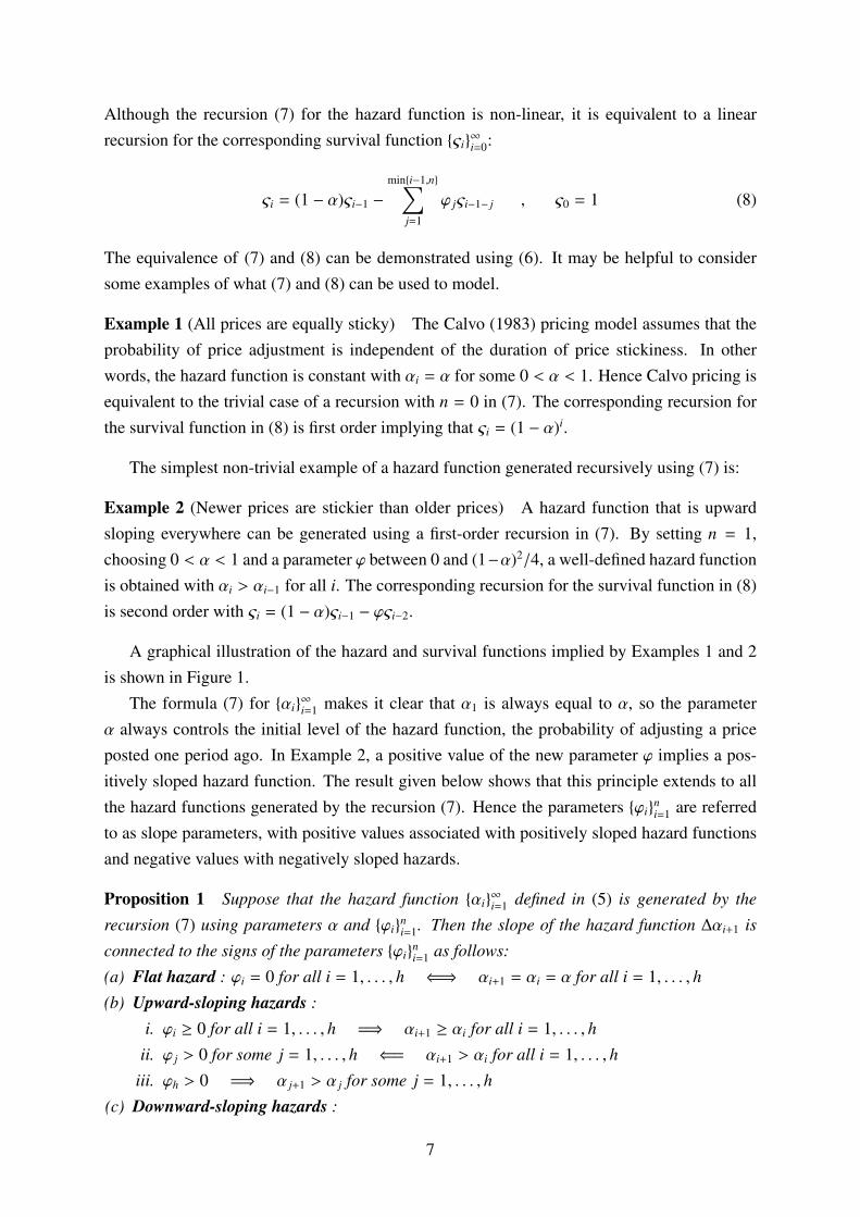
The equivalence of (7) and (8) can be demonstrated using (6). It may be helpful to considersome examples of what (7) and (8) can be used to model.

Example 1 (All prices are equally sticky) The Calvo (1983) pricing model assumes that theprobability of price adjustment is independent of the duration of price stickiness. In otherwords, the hazard function is constant with αi = α for some 0 < α < 1. Hence Calvo pricing isequivalent to the trivial case of a recursion with n = 0 in (7). The corresponding recursion forthe survival function in (8) is first order implying that ςi = (1 − α)i.

The simplest non-trivial example of a hazard function generated recursively using (7) is:

Example 2 (Newer prices are stickier than older prices) A hazard function that is upwardsloping everywhere can be generated using a first-order recursion in (7). By setting n = 1,choosing 0 < α < 1 and a parameter ϕ between 0 and (1−α)2/4, a well-defined hazard functionis obtained with αi > αi−1 for all i. The corresponding recursion for the survival function in (8)is second order with ςi = (1 − α)ςi−1 − ϕςi−2.

A graphical illustration of the hazard and survival functions implied by Examples 1 and 2is shown in Figure 1.

The formula (7) for αi∞i=1 makes it clear that α1 is always equal to α, so the parameter

α always controls the initial level of the hazard function, the probability of adjusting a priceposted one period ago. In Example 2, a positive value of the new parameter ϕ implies a pos-itively sloped hazard function. The result given below shows that this principle extends to allthe hazard functions generated by the recursion (7). Hence the parameters ϕi

ni=1 are referred

to as slope parameters, with positive values associated with positively sloped hazard functionsand negative values with negatively sloped hazards.

Proposition 1 Suppose that the hazard function αi∞i=1 defined in (5) is generated by the

recursion (7) using parameters α and ϕini=1. Then the slope of the hazard function ∆αi+1 is

connected to the signs of the parameters ϕini=1 as follows:

(a) Flat hazard : ϕi = 0 for all i = 1, . . . , h ⇐⇒ αi+1 = αi = α for all i = 1, . . . , h(b) Upward-sloping hazards :

i. ϕi ≥ 0 for all i = 1, . . . , h =⇒ αi+1 ≥ αi for all i = 1, . . . , hii. ϕ j > 0 for some j = 1, . . . , h ⇐= αi+1 > αi for all i = 1, . . . , h

iii. ϕh > 0 =⇒ α j+1 > α j for some j = 1, . . . , h(c) Downward-sloping hazards :

7

i. ϕi ≤ 0 for all i = 1, . . . , h ⇐= αi+1 ≤ αi for all i = 1, . . . , hii. ϕi < 0 for all i = 1, . . . , h =⇒ α j+1 < α j for some j = 1, . . . , h

iii. ϕ j < 0 for some j = 1, . . . , h ⇐= αh+1 < αh

Proof. See appendix A.2.

The use of the recursion (7) to generate the hazard function raises two technical questions.First, whether every hazard function satisfying the weak restrictions in Assumption 1 can berepresented by a recursion of the form (7). Secondly and conversely, whether every recursion(7) generates a hazard function satisfying Assumption 1. In brief, the respective answers areyes, approximately; and no, but restrictions on α and ϕi

ni=1 can be found to check whether

Assumption 1 is satisfied or not. These answers are justified formally by Propositions 2 and 3below.

Proposition 2 If a given hazard function αi∞i=1 satisfies all the requirements of Assumption

1 then:

(i) There exists a parameter α and a sequence ϕini=1 of some length n (possibly infinite)

such that these parameters exactly generate the original hazard function αi∞i=1 using the

recursion (7).(ii) If n = ∞ then the sequence of parameters ϕi

∞i=1 is such that limi→∞ ϕi = 0.

(iii) If α[h]i ∞i=1 is the hazard function generated by (7) but using only the first h terms of the

sequence ϕini=1, then the first h + 1 terms of α[h]

i ∞i=1 agree exactly with those of αi

∞i=1.

Proof. See appendix A.3.

Informally, Proposition 2 states that although high-order recursions are needed to repres-ent every possible hazard function, the magnitude of the extra parameters required eventuallybecomes very small, so relatively low-order recursions can approximate a wide range of differ-ently shaped hazard functions.

The second result concerns the restrictions on the parameters necessary and sufficient for thehazard function to satisfy Assumption 1. An illustrative result applying to first-order recursions(n = 1) is given below.4

Proposition 3 Suppose the hazard function αi∞i=1 is generated from parameters α and ϕ us-

ing (7) when n = 1. Then the resulting hazard function is well defined and satisfies Assumption

1 if and only if:

0 < α < 1 , −14< −α(1 − α) ≤ ϕ ≤

14

(1 − α)2 <14

(9)

Proof. See appendix A.4.

4A general result can be derived that applies to all orders of recursion, though it is more complicated to use.

8

2.3 Profit-maximizing, forward-looking price setting

When firms anticipate that the prices they set are likely to be in use for several periods, it isnecessary to balance maximizing profits today with profits in the future when selecting the bestprice. Suppose that at time t a firm posts a new money price, referred to as a reset price anddenoted by Rt. If this price is still in use at time τ ≥ t then the firm’s relative price will be Rt/Pτ

and it will earn profits z(Rt/Pτ; Yτ,Y∗τ

)in real terms at that time, where the profit function is

specified in equation (4). Future profits are discounted by financial markets using risk-freenominal interest rates.5 Future profits also have to be discounted using the survival functionςi

∞i=0 because a new price might be posted before some of these profits are actually realized.

The objective function of a firm choosing a reset price at time t is

Ft ≡ maxRt

∞∑τ=t

ςτ−tt

τ∏s=t+1

Πs

Is

z ( Rt

Pτ

; Yτ,Y∗τ

) (10)

whereΠt ≡ Pt/Pt−1 is the gross inflation rate between periods t−1 and t, It is the gross nominalinterest rate also between t − 1 and t, and t[·] is the mathematical expectation operator condi-tional on all information available at time t. The first-order condition for the profit-maximizingreset price is obtained by differentiating (10) with respect to Rt,

∞∑τ=t

ςτ−tt

τ∏s=t+1

1Is

z% ( Rt

Pτ

; Yτ,Y∗τ

) = 0 (11)

where z%(%t(ı); Yt,Y∗t

)is the derivative of the profit function (4) with respect to the firm’s own

relative price:

z%(%t(ı); Yt,Y∗t

)= (1 − ε)

1 −

ε

ε − 1%t(ı)−(1+εηcy)Y

ηcyt

%t(ı)−εYt (12)

Now let xt ≡ CY(Yt,Y∗t

)denote the level of real marginal cost in a firm producing out-

put equal to the economy-wide average Yt. An expression for firm-specific real marginal costCY

(Yt(ı); Y∗t

)is obtained from (1), which shows that xt is an increasing function of the current

output gap Yt ≡ Yt/Y∗t :

CY(Yt(ı); Y∗t

)=

(Yt(ı)Y∗t

)ηcy

, xt = Yηcyt (13)

The profit-maximizing reset price Rt is obtained by combining equations (11)–(13),

Rt = Pt

εε−1

∑∞τ=t ςτ−tt

[(∏τs=t+1

(GsΠ

εs

Is

)Π

(1+εηcy)s

)xτ

]∑∞τ=t ςτ−tt

[∏τs=t+1

GsΠεs

Is

] 1

1+εηcy

(14)

5Discounting profits using a more general stochastic discount factor would not change the results presentedhere.

9

where Gt ≡ Yt/Yt−1 denotes the gross growth rate of aggregate real output. The optimal resetprice is a weighted average of current and future real marginal costs and inflation rates. Notethat all firms choosing a reset price at the same time have an incentive to pick the same valueof Rt appearing in (14).

2.4 Aggregation

Denote the distribution of the duration of price stickiness at time t using the sequence θit∞i=0,

where θit ≡ (Dt = i) is the proportion of firms using a price set i periods ago. The definitionof the hazard function implies this distribution evolves over time according to:

θ0t =

∞∑i=1

αiθi−1,t−1 , θit = (1 − αi)θi−1,t−1 i = 1, 2, . . . (15)

If the hazard function satisfies Assumption 1 then the scope for time-variation in the distribu-tion θit

∞i=0 is transitory: there is a unique stationary distribution to which the economy must

converge.

Proposition 4 Suppose that the hazard function αi∞i=1 satisfies all the requirements of As-

sumption 1 and that the evolution over time of the distribution of the duration of price stickiness

is given by (15).(i) There exists a unique stationary distribution θi

∞i=0 to which the economy converges from

any starting point.

(ii) Now suppose the hazard function is generated by the recursion in (7) and assume that the

economy has converged to the unique stationary distribution. Then the distribution of the

duration of price stickiness is proportional to the survival function, and the unconditional

probability of price adjustment αe ≡∑∞

i=1 αiθi−1 and the unconditional expected duration

of price stickinessDe ≡∑∞

i=1 iθi−1 are given by:

θi =

α +

n∑j=1

ϕ j

ςi , αe = α +

n∑i=1

ϕi , De =1 −

∑ni=1 iϕi

α +∑n

i=1 ϕi(16)

Proof. See appendix A.5.

In what follows, the economy is assumed to have converged to the unique stationary distri-bution θi

∞i=0, so (Dt = i) = θi for all t. The price level Pt defined in (3) can then be written

in terms of a time-invariant weighted average of past reset prices:

Pt =

∞∑i=0

θiR1−εt−i

1

1−ε

(17)

10

3. Inflation dynamics

For given stochastic processes for real marginal cost xt, the growth rate of real output Gt andthe nominal interest rate It, equations (14) and (17) determine the inflation rate Πt. But as itis not generally possible to solve this system of non-linear equations analytically, the followingsection shows instead how a log-linear approximation to the solution can be found.

3.1 Steady state and log linearization

First note that equations (14) and (17) are homogeneous of degree zero in all prices expressedin money terms. These equations can then be recast in terms of the gross inflation rate Πt ≡

Pt/Pt−1 and the relative reset price rt ≡ Rt/Pt as follows:

rt =

εε−1

∑∞τ=t ςτ−tt

[(∏τs=t+1

GsΠε+(1+εηcy)sIs

)xτ

]∑∞τ=t ςτ−tt

[∏τs=t+1

GsΠεs

Is

]

11+εηcy

, 1 =

∞∑i=0

θir1−εt−i

i−1∏j=0

Πε−1t− j

(18)

It is straightforward to check that given a trend inflation rate (Πt = Π), a trend rate of outputgrowth (Gt = G) and a steady-state nominal interest rate It = I, (18) implies a well-definedsteady state for the relative reset price (rt = r) and real marginal cost (xt = x). For simplicity,the model is log-linearized around a steady state with zero inflation (Π = 1) and zero real outputgrowth (G = 1), which leads to a steady state with r = 1 and 0 < x < 1.6 The steady-state realinterest rate is assumed positive and is represented by I/Π = β−1, where β is a discount factorsatisfying 0 < β < 1.

In what follows, log deviations of variables from their steady-state values are denoted bysans serif letters. For variables that are indeterminate in the steady state, the sans serif lettersimply denotes the logarithm. The equations in (18) can be log-linearized around the steadystate defined above,

Rt =

∞∑i=0

(βiςi∑∞

j=0 βjς j

)t

[Pt+i + ηcxxt+i

], Pt =

∞∑i=0

θiRt−i (19)

where the parameter ηcx ≡ 1/(1+εηcy) represents the sensitivity of an individual firm’s marginalcost to average real marginal cost xt when it keeps its price constant.

3.2 The Phillips curve

The conventional approach to deriving the Phillips curve implied by a model of time-dependentpricing is to combine the two equations in (19), eliminate the reset price Rt, and recast theequation in terms of inflation πt ≡ Pt − Pt−1 and real marginal cost xt. This has a number

6This steady state is chosen for simplicity in many New Keynesian models. It is not difficult to extend theresults in this paper to cases where Π , 1 or G , 1.

11

of drawbacks. First, the resulting equation has a complicated autoregressive distributed lagstructure in inflation, real marginal cost, and conditional expectations of both variables subjectas many different information sets as the maximum duration of price stickiness. This makesintrinsic inflation persistence very difficult to characterize, as any inflation persistence impliedby this Phillips curve could derive from either the lags of inflation, the lags of real marginalcost, the lagged expectations of both, as well as from persistence in real marginal cost itself.Furthermore, because of the presence of expectations of the same variable conditional on manydifferent information sets, and the need for as many lags and leads of each variable as the max-imum duration of price stickiness, the Phillips curve equation is extremely difficult to estimateusing the limited-information techniques such as GMM that have proved so popular for theNew Keynesian Phillips curve.

This paper considers an simpler alternative expression for the Phillips curve which circum-vents these problems of interpretation and estimation. The key to obtaining a simple Phillipscurve is to exploit the recursive parameterization of the hazard function αi

∞i=1 in (7), which

Proposition 2 shows can be used quite generally. With this parameterization, equation (8) char-acterizes the survival function ςi

∞i=0, which implies that the equation for the profit-maximizing

reset price in (19) can be replaced by the following recursive equivalent:

Rt = β(1 − α)tRt+1 −

n∑i=1

βi+1ϕitRt+1+i +

1 − β(1 − α) +

n∑i=1

βi+1ϕi

(Pt + ηcxxt) (20)

To apply the same approach to the price level equation, note that the result in equation (16)of Proposition 4 shows that the recursive parameterization of the hazard function implies arecursion for the stationary distribution of the duration of price stickiness θi

∞i=0:

θi = (1 − α)θi−1 −

mini−1,n∑j=1

ϕ jθi− j−1 , θ0 = α +

n∑j=1

ϕ j (21)

Hence the price level equation in (19) can be replaced by the following recursive equivalent:7

Pt = (1 − α)Pt−1 −

n∑i=1

ϕiPt−1−i +

α +

n∑i=1

ϕi

Rt (22)

Solving equations (20) and (22) instead of those in (19) yields a much simpler expression forthe Phillips curve.

Theorem 1 Suppose that the hazard function αi∞i=1 satisfies Assumption 1 and is generated

by the n-th order recursion (7) with parameters α and ϕini=1. If the profit-maximizing reset

price Rt is given by equation (20) and the price level Pt by (22), and 0 < β < 1 and ηcx > 0,

then the Phillips curve relationship between inflation πt = Pt − Pt−1 and real marginal cost xt

7The translation of the equations in (19) into recursive versions (20) and (22) is essentially equivalent to findingautoregressive representations of invertible moving-average processes.

12

is:

πt =

n∑i=1

ψiπt−i +

n+1∑i=1

δitπt+i + κxxt (23)

Inflation πt depends on current real marginal cost xt, n lags of inflation and n + 1 values

of expected future inflation, where n is the order of the recursion that generates the hazard

function in (7). Note that real marginal cost can be replaced by the output gap using xt = ηcyyt,

a log-linearized version of (13). The coefficients of lagged inflation ψini=1 and future inflation

δin+1i=1 depend on the parameters α, ϕi

ni=1 and β. The coefficient κx on real marginal cost

depends on ηcx in addition to these.

The signs of the coefficients on lagged inflation are determined by the hazard function slope

parameters ϕini=1:

(a) Flat hazard : ϕi = 0 for all i = 1, . . . , n ⇐⇒ ψi = 0 for all i = 1, . . . , n(b) Upward-sloping hazards :

i. ϕi > 0 for all i = 1, . . . , n =⇒ ψi > 0 for all i = 1, . . . , nii. ϕi > 0 for some i and ϕ j = 0 for all j , i =⇒ ψ j > 0 for all j = 1, . . . , i

iii. ϕ j > 0 for some j = 1, . . . , n ⇐= ψi > 0 for some i = 1, . . . , n(c) Downward-sloping hazards :

i. ϕi < 0 for all i = 1, . . . , n =⇒ ψi < 0 for all i = 1, . . . , nii. ϕi < 0 for some i and ϕ j = 0 for all j , i =⇒ ψ j < 0 for all j = 1, . . . , i

iii. ϕ j < 0 for some j = 1, . . . , n ⇐= ψi < 0 for some i = 1, . . . , nThere are also n + 1 restrictions linking the coefficients of past inflation ψi

ni=1 and the discount

factor β to the coefficients of future inflation δin+1i=1 . These hold for all hazard functions:

δ1 = β + (1 − β)n∑

j=1

β jψ j , δi = −

βiψi−1 − (1 − β)n∑

j=i

β jψ j

i = 2, . . . , n + 1 (24)

Proof. See appendix A.6.

The key insight here is that the presence of lags of inflation in (23) is perfectly consistentwith purely forward-looking firms whenever the hazard function is not flat, that is, whenever anon-trivial recursion (7) is used with n ≥ 1. And more importantly, these lags of inflation havepositive coefficients when the hazard function is upward sloping.

The intuition for these findings can be understood by considering the effects of a shockthat initially increases inflation. Because price-adjustment times are staggered, only a subset offirm increases their prices to begin with. Since all firms that subsequently change price at thesame time choose a common reset price, those firms that did not change price at the first onsetof the shock have further to catch up than those that have already responded to the shock. Soif a larger proportion of subsequent price changes come from those firms that made no pricechange initially then the rate of inflation will be higher in the periods after the arrival of theshock. This is precisely what happens when the hazard function is upward sloping: newly set

13

prices are less likely to be changed than those that have been left fixed for a long time. Theextra inflation persistence created in this case relative to a flat hazard function is captured bythe presence of lagged inflation rates with positive coefficients.

One simple illustration of the results of Theorem 1 is given by a comparison of the Phillipscurves implied by Examples 1 and 2. In Example 1, the hazard function is completely flat,which is the key assumption of the Calvo (1983) model of sticky prices. Such a hazard functioncan be generated by the trivial case of a recursion with n = 0 in (7). In this special case,Theorem 1 simply reproduces the well-known result that the Calvo pricing model implies theNew Keynesian Phillips curve,

πt = βtπt+1 +

(α(1 − β(1 − α))ηcx

1 − α

)xt (25)

where α is the constant probability of price adjustment.8 The NKPC states that inflation de-pends only on the current level of real marginal cost and expected inflation one period in thefuture, and it has attracted criticism because it lacks any role for past inflation. A popular al-ternative empirical specification, which nests the NKPC, is the so-called hybrid New KeynesianPhillips curve (HNKPC):

πt = bpπt−1 + b ftπt+1 + bxxt (26)

This alternative Phillips curve postulates that past inflation is an explicit determinant of currentinflation, but it has proved more difficult to find a readily acceptable theoretical foundation forbp > 0 in (26).

Now consider the upward-sloping hazard function of Example 2 again. It is generated by afirst-order hazard function recursion using two parameters α and ϕ, with the former controllingthe level of the hazard function and the latter its slope. According to Theorem 1, the Phillipscurve in this case takes the form:

πt = ψπt−1 + β(1 + (1 − β)ψ)tπt+1 − β2ψtπt+2 + κxxt (27)

Current inflation now depends directly on past inflation, along with real marginal cost andexpected inflation one and two periods in the future. Apart from the second future inflationterm, (27) has the same form as the hybrid New Keynesian Phillips curve (26), but unlike thelatter, it has a clear theoretical foundation.

The coefficient ψ determines the weight attached to past inflation relative to expected futureinflation in influencing current inflation. When β is close to one, the weights on past andfuture inflation are approximately ψ and 1 − ψ respectively. A positive value of ψ means thatcurrent inflation depends positively on lagged inflation and that the weight on future inflation isreduced, though remaining positive if ψ < 1. While expected inflation two periods in the future

8See Woodford (2003) for a detailed derivation of the NKPC and further discussion.

14

then has a negative coefficient, it should not be interpreted as implying that higher expectedinflation two periods ahead lowers inflation today. This is because the Phillips curve (27) attime t + 1 implies that a rise in inflation in period t + 2 creates a similar amount of inflationarypressure in period t + 1. The sum of the coefficients on both future inflation terms is positiveif ψ < 1, so in this case the expected inflation in period t + 2 would still raise inflation today,albeit by less than when ψ = 0. Therefore the negative coefficient on expected inflation twoperiods in the future should be interpreted only as a reduction in the overall weight attached tofuture inflation.

The coefficient ψ of lagged inflation and the coefficient κx of real marginal cost are obtainedfrom the following functions of the parameters α, ϕ, β and ηcx:

ψ =ϕ

(1 − α) − ϕ(1 − β(1 − α)), κx =

(α + ϕ)(1 − β(1 − α) + β2ϕ)ηcx

(1 − α) − ϕ(1 − β(1 − α))(28)

For the underlying hazard function to be well defined, the inequalities in (9) involving theparameters α and ϕ must be satisfied. These guarantee that κx is always positive, and that thesign of ψ depends only on the sign of ϕ. As Proposition 1 shows that ϕ > 0 implies a hazardfunction that is positively sloped everywhere, it is seen that this type of hazard function leadsto a Phillips curve in which lagged inflation has a positive coefficient ψ > 0. The magnitude ofthis coefficient is increasing in the hazard-function slope parameter ϕ.

The principle that a positively sloped hazard function is associated with positive coefficientsof lagged inflation generalizes to richer models with more parameters. This is because the sameset of parameters ϕi

ni=1 controls both the slope of the hazard function according to Proposition

1, and the signs of the coefficients of lagged inflation in the Phillips curve (23) according toTheorem 1. This is the key theoretical result contained in this paper, which is stated belowformally:

Corollary 1 Suppose firms maximize profits (10) when they set prices and that the hazard

function for price adjustment αi∞i=1 satisfies Assumption 1.

(i) There exists a class of hazard functions that are everywhere upward sloping and which

imply that all the coefficients of past inflation in the Phillips curve (23) are positive.

(ii) If one or more of the coefficients of lagged inflation in the Phillips curve (23) is positive

then the hazard function must have one or more upward-sloping sections.

Proof. These claims follow immediately from Propositions 1 and 2 together with Theorem1.

Thus by constructing a hazard function using (7) with all the ϕi parameters positive, it is pos-sible to explain any number of positive coefficients of lagged inflation. In fact, as Proposition 1and Theorem 1 show, an appropriate choice of signs for the parameters ϕi

ni=1 can generate es-

sentially any pattern of signs for the sequence of coefficients of past inflation. Therefore, on itsown, the hypothesis of time-dependent pricing with forward-looking, profit-maximizing firms

15

has no implications for the signs of the coefficients of past inflation. But when combined witha hypothesis about the shape of the hazard function, there are clear implications for the signs ofthese coefficients. Corollary 1 shows that there are hazard functions which are upward slopingeverywhere that imply Phillips curves in which every coefficient of lagged inflation is positive.This sufficiency result is complemented by a corresponding necessity result. If at least one ofthe coefficients of lagged inflation is positive and firms are forward-looking profit maximizersthen the hazard function must be positively sloped somewhere. It follows immediately thatif the hazard function were everywhere downward sloping then all the coefficients on laggedinflation would be unambiguously negative.

4. Estimating the hazard function

The analysis in section 3 demonstrates that the shape of the hazard function is systematicallyrelated to inflation dynamics. By exploiting this insight it is possible to devise a method forestimating the hazard function that requires only macroeconomic data and simple econometrictechniques. No individual price observations are needed. This method is used to answer thequestion of whether a hazard function model can be found that is quantitatively as well asqualitatively consistent with the behaviour of inflation. The results are also compared withthose derived from the more conventional microeconometric approach.

4.1 Estimation method and specification issues

An observable proxy for real marginal cost

It is first necessary to find some observable proxy for the driving variable xt in the Phillipscurve (23), that is, for the level of real marginal cost in the average firm. One solution is toreplace it with the output gap yt, which then in practice could be equated with the deviation ofaggregate output from some trend. This approach is eschewed here for a number of reasons.First, the link between average real marginal cost and the output gap derived in section 3.1 maychange in the presence of features such as sticky wages or risk-sharing employment contractsfrom which this paper has abstracted. Second, there are many different detrending proceduresfor aggregate output and thus a range of “output gap” measures to choose from. It is difficultto know which statistical detrending procedure, if any, delivers a measure consistent with thetheoretical concept of the output gap required by the model.

An alternative approach that has become popular in work on the New Keynesian Phillipscurve is to use (real) unit labour costs in place of real marginal cost (Galı and Gertler, 1999;Sbordone, 2002). Unit labour costs have the advantage of being readily measurable withoutthe need for detrending. Justifying the substitution of unit labour costs for real marginal costrequires a few more assumptions beyond those introduced in section 2.1. Assume each firmı ∈ Ω in the economy faces a Cobb-Douglas production function Yt(ı) = AtHt(ı)ηyh . Firm ı

16

produces output Yt(ı) by using Ht(ı) hours of a homogeneous labour input. The term At capturesexogenous technological progress, and the parameter ηyh measures the elasticity of output withrespect to hours and is assumed to satisfy 0 < ηyh ≤ 1. Firms can hire as many hours of labouras they want at real wage wt.

It is not difficult to show that the Cobb-Douglas production function and the assumptionthat firms are wage takers implies that the total real cost function C

(Yt(ı); Y∗t

)takes the form

given in equation (1), with parameter ηcy = (1 − ηyh)/ηyh measuring the elasticity of firms’ realmarginal cost with respect to their own output. If Ht is the total number of hours supplied by allworkers then the combination of the labour market equilibrium condition, the individual Cobb-Douglas production functions for each firm and the demand curves in (3) implies an aggregateproduction function Yt = At(Ht/∆t)ηyh , where ∆t is an index of relative-price dispersion.

Average real marginal cost is defined by xt ≡ CY(Yt,Y∗t

), and given the aggregate production

function and (13) it follows that xt = (wtHt)/(ηyhYt∆t). Hence if t ≡ wtHt/Yt is the labour shareof income then xt = t/(ηyh∆t). Since the first-order terms of a Taylor expansion of ∆t aroundthe steady state defined in section 3.1 are all zero, the log deviation xt of real marginal cost fromits steady-state value is equal to the log deviation st of the labour share, ignoring second- andhigher-order terms. In the data, unit labour costs are defined as labour compensation dividedby output, so when expressed in real terms this measure is equivalent to the labour share ofincome, and hence to real marginal cost, under the assumptions made in this section.

Identification

The approach to identifying the hazard function αi∞i=1 using macroeconomic data relies on the

connection between the coefficients ψini=1, δi

n+1i=1 and κx appearing in the Phillips curve (23)

and the hazard function parameters α and ϕini=1.

Suppose first that the Phillips curve coefficients are identified. There are 2(n + 1) of thesecoefficients, and n + 3 underlying parameters to be identified, namely α, ϕi

ni=1, β and ηcx. A

result of Theorem 1 is that each inflation coefficient ψi or δi is a function of α, ϕini=1 and the

discount factor β. But the mapping between the coefficients and the parameters is non-linear,and it turns out that if any subset of size n of ψi

ni=1 and δi

n+1i=1 is known then the remaining

n + 1 coefficients can be inferred given the value of β. So in total, the Phillips curve coefficientsprovide only n + 2 independent pieces of information about the parameters and thus an extrarestriction is needed.

This extra information is provided by a calibration of the elasticities ε and ηcy, which pinsdown ηcx = 1/(1 + εηcy). The equations in (18) imply ε/(ε − 1)x = 1, where x is steady-statereal marginal cost. It follows that the model generates an average markup on marginal cost of1/(ε − 1). By combining this result with the analysis from the previous sub-section, the modelis seen to imply an average labour share of income of (ε− 1)/(ε(1 + ηcy)). The average markupis set to 20%, which implies a price elasticity of demand ε = 6. With the average labour

17

share equal to 67%, an elasticity of real marginal cost with respect to output of ηcy = 0.25 isrequired. It follows that ηcx = 0.4. As a robustness check, the special case of ηcx = 1 is alsoconsidered. This was originally the only case considered in Galı and Gertler’s (1999) work onthe New Keynesian Phillips curve. The subsequent study by Galı, Gertler and Lopez-Salido(2001) considers both ηcx = 1 and 0 < ηcx < 1. From the results derived earlier, it is apparentthat ηcx = 1 requires ηcy = 0, which is equivalent to no diminishing returns to labour in theshort run. This seems implausible, so ηcx = 0.4 is the preferred choice here.

Even if the hazard function parameters α and ϕini=1 are identified, there is no guarantee

that their estimated values will automatically imply a well-defined hazard function. Theorem1 reveals that a hazard function satisfying Assumption 1 generated by (7) using α and ϕi

ni=1

necessarily implies a Phillips curve of the form (23) for some coefficients ψini=1, δi

n+1i=1 and κx.

But the converse is not true for the hazard function parameters recovered from any arbitrary setof Phillips curve coefficients. However, once the parameters are estimated, it is possible to testwhether the implied hazard function is well defined or not.

The foregoing discussion assumes that the coefficients in the Phillips curve (23) are them-selves identified. Suppose the Phillips curve equation (23) holds with an error term νt ∼

IID(0, σ2ν), and that real marginal cost xt is replaced by the observable labour share of in-

come st (real unit labour cost) as explained earlier. If the expected future inflation rates arereplaced by their realized values then the Phillips curve equation becomes πt =

∑ni=1 ψiπt−i +∑n+1

i=1 δiπt+i + κxst + υt, where υt ≡ νt −∑n+1

i=1 δieit+i is a composite error term that depends on the

i-step ahead prediction errors eit ≡ πt − t−iπt.

At time t, the variables st , πt , . . . , πt+n+1 are endogenous and non-predetermined,so instruments are required to achieve identification of all the coefficients. Let zt−1 be a q × 1vector of observable variables that are known by firms at time t − 1. If firms do not makepredictable errors when forecasting inflation then υt should be uncorrelated with zt−1, implyingthe following moment conditions involving the coefficients ψi

ni=1, δi

n+1i=1 and κx:

πt −

n∑i=1

ψiπt−i −

n+1∑i=1

δiπt+i − κxst

zt−1

= 0 (29)

Identification of the hazard function parameters α and ϕini=1 and the discount factor β therefore

requires there to be at least n + 2 variables in zt−1 that have predictive power for the current andfuture endogenous variables appearing in (23). However, since the underlying theory itselfimplies that inflation is given by (23), n lags of inflation can always be included in zt−1. Thisleaves only two other variables to be found with the necessary predictive power.

Econometric technique

A limited-information approach is employed here to estimating the hazard function using asingle Phillips curve equation. In particular, a generalized method of moments (GMM) estim-

18

ator is applied using the moment conditions in (29).9 The methodology mirrors that used byGalı and Gertler (1999) to estimate the New Keynesian Phillips curve.10

The hazard function parameters α and ϕini=1 are estimated using the moment conditions

in (29) and the link with the Phillips curve coefficients ψini=1, δi

n+1i=1 and κx provided by The-

orem 1. This means that the coefficients appearing in the moment conditions (29) are actuallynon-linear functions of the estimated parameters, and so the issue of the normalization of themoment conditions must be addressed. In small samples, the choice of normalization can affectthe results. Rather than taking the moment conditions as they are in (29), these conditions aremultiplied by a function of the parameters that ensures the resulting Phillips curve coefficientsare bounded whenever the set of parameters α and ϕi

ni=1 is bounded.11 The alternative normal-

ization that leaves (29) unchanged, which imposes a coefficient of one on current inflation, isused as a robustness check. An equivalent pair of normalizations is also considered by Galı andGertler (1999), who claim that the bounded normalization is shown by simulation studies tohave better small-sample properties than the normalization with a coefficient of one on currentinflation. So the bounded normalization is the preferred specification here and is denoted byN(1). The alternative normalization on current inflation is denoted by N(2).

The GMM estimator applied in this paper uses a four-lag Newey-West estimator of theoptimal weighting matrix for the moment conditions. For each weighting matrix, the numer-ical minimization algorithm for the criterion function is iterated until convergence because thecoefficients in the moment conditions are non-linear functions of the parameters. The resultingestimates are then used to update the weighting matrix, and the process is repeated until theweighting matrix converges itself. Robust standard errors of the parameter estimates are alsoobtained using a four-lag Newey-West estimator of the variance-covariance matrix.12

Data

Quarterly U.S. data from 1960:Q1 to 2003:Q4 are used.13 Inflation is measured by the annu-alized percentage change in the GDP deflator between consecutive quarters. Real unit labourcosts are given by unit labour costs in the business sector divided by the GDP deflator, andexpressed as a percentage deviation from their average value. The GMM estimation procedurerequires that instruments be found for the current and future endogenous variables appearing inthe Phillips curve. The lags of the following variables were selected for this role in addition tolags of inflation and unit labour costs themselves: the spread between ten-year Treasury Bond

9The estimation is performed using Cliff’s (2003) GMM package for MATLAB.10The alternative of full-information maximum likelihood estimation is not pursued here since it would require

a complete model of the data-generating process, and would be less robust than GMM if this were misspecified.For maximum likelihood estimation of the NKPC, see Linde (2005) and Kurmann (2004).

11The requisite factor is the expression in the denominators of the coefficients ψini=1, δi

n+1i=1 and κx, as given in

the block of equations (A.4) from the proof of Theorem 1.12For more details on different GMM estimation methods, see Matyas (1999).13The source of the data is the Federal Reserve Economic Data (FRED) database, which is available online at

research.stlouisfed.org/fred2.

19

and three-month Treasury Bill yields, quadratically detrended log real GDP, the rate of wageinflation (annualized percentage change in compensation per hour in the business sector), andthe rate of commodity-price inflation as measured by the percentage change between consec-utive quarters of a futures-price index. These are very similar to the instruments used in theoriginal Galı and Gertler (1999) study of the NKPC. Based on their statistical significance ina predictive regression for future inflation, six lags of inflation and commodity-price inflationare selected as instruments, together with two lags of each of the other variables.

4.2 Estimation results

To establish a benchmark with which later results can be compared, the hazard function isfirst estimated when it is constrained to be flat, as in Example 1. This is the Calvo pricingmodel underlying the standard New Keynesian Phillips curve. It is obtained by imposing n = 0in the hazard function recursion (7). There are just two parameters to estimate: the constantprobability of price adjustment α and the discount factor β. The parameter ηcx is calibrated asdiscussed in section 4.1. Estimates are presented in Table 1 for all pairings of the calibratedvalues of ηcx and the normalizations of the moment conditions detailed in section 4.1. Thepreferred specification is ηcx = 0.4 and N(1).

The constant probability of price adjustment is found to be 0.405 per quarter under thepreferred specification ηcx = 0.4 andN(1). This is quite high, though by no means inconsistentwith the micro-level evidence on price adjustment. As (25) shows, the coefficient of futureinflation is determined entirely by the discount factor β. The estimates of β are not significantlydifferent from one in any specification. The coefficient of unit labour costs st (the labour share)is positive and significant at the 5% level when the preferred normalizationN(1) is used. Noticethat the standard errors tend to be larger when normalization N(2) is used. As the hazardfunction is constrained to be flat, the estimates of the expected probability of price adjustmentαe are identical to the parameter α itself. The expected duration of price stickiness De iscalculated using (16) and is found to be 2.469 quarters under the preferred specification. Underthe alternative specifications, the expected duration is estimated to be noticeably longer. Finally,none of the J-statistics reports a rejection of the over-identifying moment conditions.14

The estimated hazard and survival functions for the Calvo model are plotted in Figure 2.These are derived from the estimated parameters under the preferred specification in Table 1.The hazard function is of course necessarily flat and the survival function decays at a con-stant geometric rate, as was first seen for Example 1 in Figure 1. The thick and thin bars inFigure 2 represent one-standard-deviation and two-standard-deviations bands around the pointestimates.

The aim is now to use macroeconomic data to estimate the shape of the hazard function,imposing as few a priori restrictions as possible on what shapes are admissible. A first step

14The J-statistic is the Hansen test of over-identifying restrictions derived from surplus moment conditions. SeeMatyas (1999) for further details.

20

towards this goal is taken by estimating a hazard function with both a level parameter α andone slope parameter ϕ1. This is done by considering hazard functions in the class generatedby first-order recursions, as illustrated by Example 2. This allows monotonically increasinghazard functions to be accommodated, and these have been seen to generate Phillips curves inwhich lagged inflation has a positive coefficient.

The estimation results for the parameters α, ϕ1 and β of the first-order recursive model aredisplayed in Table 2. What is immediately apparent is that the estimates of ϕ1 are positive andstatistically significant at the 5% level for all specifications. This represents a strong rejection ofthe Calvo model, which is equivalent to the null hypothesis ϕ1 = 0 within this class of models.By invoking the results of Proposition 1, the point estimates of ϕ1 imply a hazard function thatis increasing everywhere. The parameter α now needs to be interpreted differently from theCalvo model results in Table 1. Here it is merely the probability of a firm changing a price thatwas posted at some time during the previous quarter. The estimates of α in Table 2 are muchlower than those in Table 1, and are not significantly different from zero in any case. In theother columns of Table 2, the estimates of β are quite low but insignificantly different from one.The J-statistics fail to reject the over-identifying restrictions in any specification.

As discussed in section 4.1, the restrictions on the parameters α and ϕ1 needed to ensurethat the implied hazard function is well defined are not imposed at the estimation stage. Therationale for doing this is to allow these theoretical restrictions to be tested and thus assesswhether inflation dynamics are consistent with a well-defined hazard function model. Propos-ition 3 shows that for the first-order model, the restrictions are given by the inequalities in (9).The first of these is 0 < α < 1. The estimate from the preferred specification passes this test,and while the point estimates under the alternative specifications fail to do so, none of the viol-ations is statistically significant. The next condition from (9) to check is given as (1−α)2/4−ϕ1

in a column of Table 2. According to (9), this should be positive if the hazard function is to bewell defined everywhere. There are small and statistically insignificant violations of this con-dition in three out of the four specifications considered in Table 2. The third condition requiredby (9) is automatically satisfied because all the point estimates of ϕ1 are positive.

Plots of the implied hazard and survival functions for the estimated first-order recursivemodel are shown in Figure 3. As usual, these are plotted for the parameters estimated under thepreferred specification, that is, the first row of Table 2. The hazard function is upward slopingbecause the point estimate of ϕ1 is positive. The one- and two-standard-deviation bands inFigure 3 imply that the estimated hazard function starts at a point insignificantly different fromzero (given by the parameter α) for prices that have been changed very recently, and rises toa point insignificantly different from one for prices that have been left fixed for six or sevenquarters. Because the estimated parameters fail to satisfy all the inequalities in (9), the pointestimate of the hazard function is not well defined beyond seven quarters. The bands alsobecome very wide as the duration of price stickiness increases.15 In spite of the wide bands,

15This should not be surprising. Once the proportion of firms using a price of a particular age shrinks to zero

21

hypotheses about the slope of the hazard function can be tested directly using the sign of theparameter ϕ1 as discussed above.

The coefficients of the implied Phillips curve for the first-order model are given in Table3. The key point to note is that the significantly positive ϕ1 parameter from Table 2 trans-lates into a significantly positive coefficient on inflation lagged one quarter. Thus the estimatedhazard function shown in Figure 3 implies a non-negligible amount of intrinsic inflation per-sistence, comparable in magnitude to that found by Galı and Gertler (1999) for a model withbackward-looking firms. The parameter estimates also imply a significantly negative coeffi-cient on expected inflation two quarters in the future, but the coefficient on inflation one quarterahead remains significantly positive. As has been discussed, this negative coefficient shouldbe interpreted merely as a reduction of the weight attached to future inflation in determiningcurrent inflation. In the preferred specification, the coefficient on unit labour costs is positiveand statistically significant at the 5% level.

It is interesting to note that the estimated first-order model is able to generate intrinsicinflation persistence without requiring noticeably more price stickiness than is found in theestimated Calvo model. While the expected probability of price adjustment αe is estimatedto be larger in the Calvo model, Tables 1 and 2 show that the average duration De of pricestickiness is 2.198 quarters for the first-order model and 2.469 quarters for the Calvo model.Inspection of the hazard functions in Figures 2 and 3 shows that the hazard function for thefirst-order model is above that of the Calvo model for all prices except those posted in theprevious quarter.

On the basis of the results for the first-order recursive model, a flat hazard function is clearlyrejected by the data in favour of an alternative with a monotonically increasing hazard function.This new model offers a more promising account of inflation dynamics. However, restrictingattention to hazard functions generated by a first-order recursion in (7) still imposes essentiallyarbitrary limitations on the range of allowed hazard function shapes. For this reason, it isdesirable to consider higher-order models. Proposition 2 shows that if the true hazard functionsatisfies Assumption 1 and if n is made sufficiently large then a recursion of the form (7) is ableto approximate the model as accurately as is required. But econometric practicalities put somelimits on the maximum order of model that can be estimated because the number of terms inthe Phillips curve (23) rises in step with the order of the recursion.

Starting from n = 2, progressively higher orders of recursion (7) were estimated. The extraparameter ϕ2 introduced by the second-order model turns out to be statistically insignificant.More success is had with the cases n = 3 and n = 4 where both ϕ3 and ϕ4 are highly significant.Beyond that, no additional statistically significant slope parameters are found, with models upto n = 8 being estimated. The full set of results is not reported here owing to limited space, butthe fourth-order model is presented as typical of these findings. The estimates of the parameters

the probability of such a price being changed ceases to be identified. The Calvo model avoids this problem byasserting the probability is the same for prices of all ages.

22

α, ϕi4i=1 and β are displayed in Table 4.

The initial probability of price adjustment α is estimated to be low and insignificantly dif-ferent from zero in all specifications. The slope parameters ϕ1 and ϕ4 are found to be signi-ficantly positive; ϕ2 is insignificantly different from zero, and ϕ3 is significant and negative.The mixture of positives and negatives suggests that the implied hazard function is no longermonotonic. This is confirmed by the plots of the hazard and survival functions in Figure 4. Thepoint estimate of the hazard function begins at a point insignificantly different from zero forprices that have just been set, and begins to rise during the first and second quarters of a spellof price stickiness. It falls back in the third quarter and then rises again in the fourth quarter. Atthe beginning of the second year of price stickiness the hazard function rises sharply, but againfalls back somewhat after the middle of the second year. Finally, it rises very sharply againafter around two years of price stickiness, reaching a level not significantly different from one.These results suggest that firms are more likely to make a price adjustment around the first andsecond anniversaries of their previous price change: a feature that also finds some support in themicro evidence. After a duration of two years, the hazard function is estimated too impreciselyto draw any firm conclusions.

As is the case with the estimated first-order model, the point estimate of the fourth-orderhazard function in Figure 4 is well defined for most, but not all, durations of price stickiness.The most prominent failure is in the fourth quarter where the point estimate dips below zero,but this deviation is not statistically significant. The estimates of the hazard function after theeighth quarter are much too loose to be able to detect any statistically significant deviation hereeither. Therefore, the estimated fourth-order model is very close to implying a well-definedhazard function, and no statistically significant failure to meet this requirement can be found.

The implied Phillips curve for the estimated fourth-order model is exhibited in Table 5. Thefirst and the fourth lags of inflation now have significantly positive coefficients, the second lag’scoefficient is a small and insignificant positive number, and the third lag has a negative coef-ficient that is statistically significant. Overall, the positive coefficients on the lags of inflationclearly dominate. Thus the hazard function in Figure 4 provides a rationale for why inflationrates one quarter ago and one year ago contribute positively to intrinsic inflation persistence.Among the coefficients on future inflation there is a mixture of positives and negatives. In thepreferred specification, the coefficient of unit labour costs remains positive and significant atthe 10% level.

The conclusions drawn from these results are: that a flat hazard function is resoundinglyrejected; that hazard functions with upward sloping sections are found; that these can justifythe quantitative importance of the positive coefficients of lagged inflation found for estimatedPhillips curves; that although the estimated hazard functions are not well defined for all dura-tions of price stickiness, no statistically significant rejection of a well-defined hazard functionis found.

23

4.3 Comparison with the microeconometric evidence

There are now many studies that estimate the hazard function for price adjustment using mi-croeconomic data on individual prices (Baumgartner et al., 2005; Campbell and Eden, 2005;Cecchetti, 1986; Dias et al., 2005; Fougere et al., 2005; Gotte et al., 2005; Nakamura andSteinsson, 2007). There are a range of findings in this literature. Papers such as Gotte et al.(2005) and Cecchetti (1986) find strong evidence in favour of an upward-sloping hazard func-tion. Both papers use a small number of goods, but have data spanning several decades. Otherssuch as Campbell and Eden (2005) and Dias et al. (2005) find strong evidence that the hazardfunction is downward sloping. Some studies such as Baumgartner et al. (2005) agree that thehazard function is generally downward sloping, but find that the negative slope is interruptedby sharp spikes at regular intervals. This group of studies uses data on a very large number ofgoods, but these data are drawn from a relatively small number of years in the last decade.

It is argued that some of the findings of downward-sloping hazards can be explained asthe result of a heterogeneity bias (Alvarez et al., 2005). Many studies include a wide rangeof products that have different degrees of price stickiness. Heterogeneity biases estimates ofthe hazard function slope downward because goods with more flexible prices are less likelyto be found to have long spells of price stickiness.16 As a result of this criticism, studiessuch as Nakamura and Steinsson (2007) and Fougere et al. (2005) take careful steps to controlfor heterogeneity. Nakamura and Steinsson (2007) allow the level of each product’s hazardfunction to be different. They find that the estimated hazard function is then largely flat, with alarge spike after one year. Fougere et al. (2005) allow both the level and the slope of the hazardfunction to differ across products. The results are now mixed, with a range of increasing anddecreasing hazards found for different goods and different types of retail outlet. But increasinghazard functions are in the majority.

If the results based on macro data from section 4 are compared only with those microecono-metric studies that span several decades including times of high as well as low inflation, thenthere is no contradiction between the micro and macro evidence. However, the micro studiesin this group draw on a rather narrow range of goods, though on the other hand this narrowrange may also be a virtue if the heterogeneity bias is thought to be a serious problem. Evid-ence from the more comprehensive micro studies working with data from the 1990s and 2000sdoes present a prima facie contradiction to the macro-data estimates of hazard functions for theperiod 1960–2003 derived in this paper. There are two points to bear in mind here. First, itremains to be seen how robust the finding of a downward-sloping hazard function is once het-erogeneity is properly controlled for. Second, the theoretical case for an upward-sloping hazardfunction is strongest in periods of higher inflation, hence the hazard function slope may not bea structural feature of the economy. Thus the failure to find a positive slope using data only

16See Heckman and Singer (1984) and Kiefer (1988) for more discussion of the problem of heterogeneity induration analysis.

24

from a period of low and stable inflation may not be surprising.17 Finally, it should be notedthat hazard function “spikes” found in the microeconometric literature are of course evidencefor a sharply upward-sloping section of the hazard function, and thus contribute to explainingintrinsic inflation persistence. The fact that the spikes also imply a sharply downward-slopingsection does not offset this effect because the existence of a spike at some duration implies thatmuch fewer price spells survive beyond that duration to where the hazard function is actuallydownward sloping.

5. Conclusions

This paper has studied the link between intrinsic inflation persistence and the price-setting be-haviour of firms. Intrinsic inflation persistence refers to inflation that occurs purely as a resultof past pricing decisions and cannot be explained by current and expected future fundamentalssuch as unit labour costs, output gaps, monetary policy, or cost-push shocks. When intrinsicinflation persistence is present in an economy, it is not possible for the central bank to bring in-flation immediately back to target without some loss of output, even if the shocks that gave riseto the inflation have dissipated. Most empirical studies conclude that inflation determination isnot a purely forward-looking process and that inflation contains a significant backward-lookingcomponent, though the reasons for the existence of this intrinsic inflation persistence are con-sidered to be a puzzle. But the results of this paper show that there is no contradiction betweensuch persistence and profit-maximizing, forward-looking price setting by firms.

What turns out to be important for intrinsic inflation persistence is not how much pricestickiness there is on average, but whether there are systematic differences between the sticki-ness of prices of different ages. In particular, newer prices need to be stickier than older pricesin order to explain this persistence. If older prices are more likely to be adjusted then the“catch-up” effect of firms whose prices have remained fixed for a long time has a larger impacton current inflation than the “roll-back” effect of firms who have recently adjusted their pricesafter a shock, leading to sustained rises in the price level even following temporary shocks.

In terms of the hazard function for price changes, the most important feature influencingintrinsic inflation persistence is the slope, not the level. The level could be very high or verylow, representing the extremes of price flexibility or stickiness, but as long as the hazard func-tion remains flat there can be no intrinsic persistence. To provide a rationale for the type ofintrinsic inflation persistence described above, where high inflation in the past makes it harderto achieve low inflation today without sacrificing output, it is necessary that the hazard func-tion is predominantly upward sloping. If the hazard function were predominantly downwardsloping then a perverse result is obtained whereby the higher inflation has been in the past, the

17A preliminary subsample analysis (not reported here) suggests that macro-based estimates of the hazard func-tion using only data from the mid 1980s to 2000s find a hazard function that is initially downward sloping andfollowed by less steeply upward-sloping sections.

25

easier it is to achieve low inflation today without cost.In order to study the link between the hazard function for price changes and intrinsic in-

flation persistence, a methodological innovation is introduced that shows how essentially allhazard functions have a recursive representation. This allows much simpler expressions to beobtained for the Phillips curves implied by non-constant hazard models of price setting. Theresulting class of simple Phillips curves closely resembles the “hybrid” New Keynesian Phil-lips curves widely used in empirical work and policy analysis, but which are thought to haveweak theoretical foundations because they introduce lags of inflation arbitrarily that are notpresent in the standard New Keynesian model. But there is nothing arbitrary about these lags:they are simply the implication of profit-maximizing behaviour by firms when the likelihoodof adjusting prices depends on the amount of time elapsed since the previous price change. Byusing this new class of Phillips curves, intrinsic inflation persistence can be precisely defined interms of the coefficients of lagged inflation. It is shown analytically how positively sloped haz-ard functions imply positive values of these coefficients and negatively sloped hazards implythat these coefficients have negative values.

By building on these insights, this paper then sets out a method for estimating the haz-ard function for price changes without needing microeconomic data on individual prices. Thehazard function can be identified and estimated using only macroeconomic time-series on in-flation and unit labour costs and simple econometric techniques. The results of this exercisestrongly reject the flat hazard function underlying the standard New Keynesian Phillips curve.The point estimates suggest that the hazard function is predominantly upward sloping, start-ing from a probability of price adjustment not significantly different from zero for prices thathave been changed very recently, rising to a probability not significantly different from onefor prices that have remained sticky for eight or more quarters. In between, the hazard func-tion initially rises and then falls back during the first year of price stickiness. There is then asudden increase in the probability of price adjustment towards the end of the first year and thebeginning of the second year. A similar sudden rise is also found towards the end of the secondyear. No statistically significant rejection of a well-defined hazard function is found. Therefore,in summary, an upward-sloping hazard function model offers a significantly better account ofempirical inflation dynamics without introducing any arbitrary backward-looking behaviour.

26

Table 1Estimates of the Calvo pricing model (n = 0)

Specification§ α β αe] De] J-stat‡ Etπt+1\ xt

\

ηcx = 0.4 0.405** 0.966** 0.405** 2.469** 17.223 0.966** 0.116**

N(1) (0.053) (0.028) (0.053) (0.322) [0.575] (0.028) (0.040)

ηcx = 0.4 0.217** 0.985** 0.217** 4.601** 14.804 0.985** 0.025N(2) (0.106) (0.024) (0.106) (2.246) [0.735] (0.024) (0.028)

ηcx = 1.0 0.226** 0.975** 0.226** 4.432** 15.873 0.975** 0.071**

N(1) (0.046) (0.026) (0.046) (0.895) [0.666] (0.026) (0.033)

ηcx = 1.0 0.142* 0.985** 0.142* 7.064* 14.804 0.985** 0.025N(2) (0.073) (0.024) (0.073) (3.637) [0.735] (0.024) (0.028)

Notes: Estimation of the parameters α and β is by GMM using U.S. quarterly data 1960:Q1–2003:Q4. The moment conditions are given in (29) and the data are described in section 4.1.The estimators of the parameters and the GMM weighting matrix are sequentially iterated untilconvergence. A four-lag Newey-West estimator of the optimal weighting matrix and the standarderrors is used. Standard errors are given in parentheses, and are calculated using the delta methodfor non-linear functions of the estimated parameters.

* Statistically significant at the 10% level.** Statistically significant at the 5% level.§ Each specification is a calibrated value of the parameter ηcx and a choice of either normalizationN(1) or N(2). See section 4.1 for further details.

] The expected probability of price adjustment αe and the expected duration of price stickiness De

are inferred from the estimated parameters using equation (16).‡ This is the Hansen test of over-identifying moment conditions. The p-value is in brackets.\ These are the implied coefficients of the New Keynesian Phillips curve in (25).

27

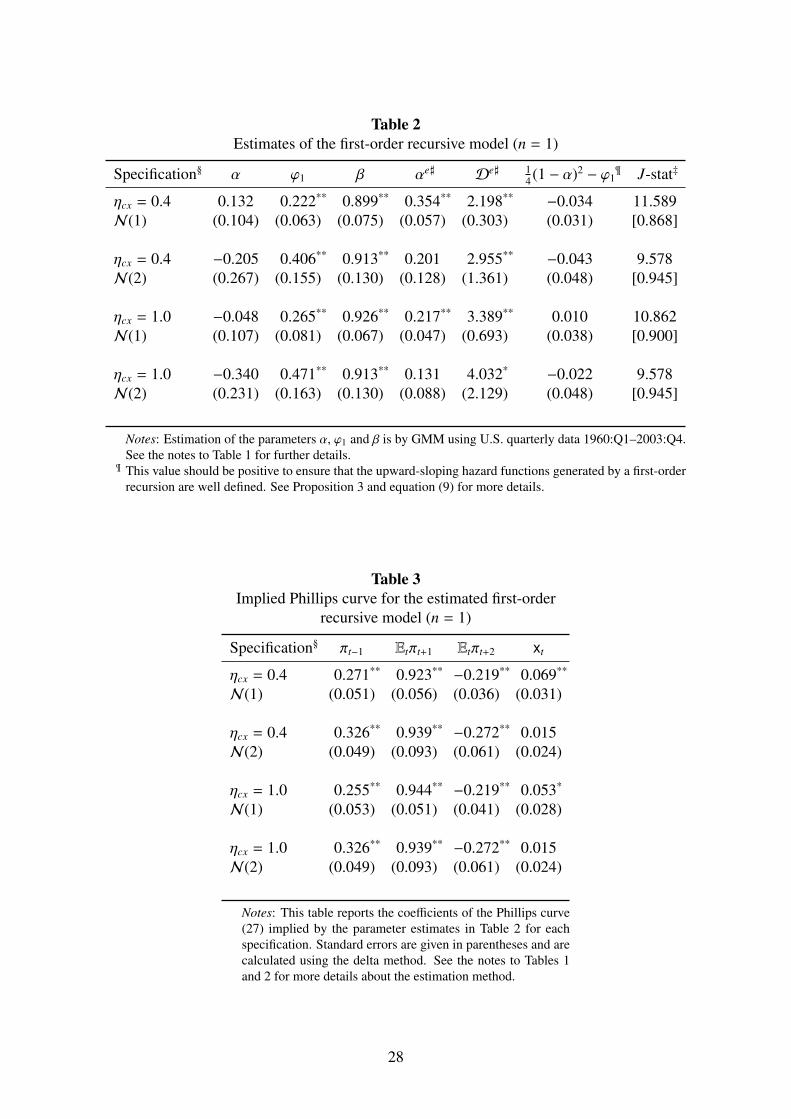
Table 2Estimates of the first-order recursive model (n = 1)

Specification§ α ϕ1 β αe] De] 14 (1 − α)2 − ϕ1

¶ J-stat‡

ηcx = 0.4 0.132 0.222** 0.899** 0.354** 2.198** −0.034 11.589N(1) (0.104) (0.063) (0.075) (0.057) (0.303) (0.031) [0.868]

ηcx = 0.4 −0.205 0.406** 0.913** 0.201 2.955** −0.043 9.578N(2) (0.267) (0.155) (0.130) (0.128) (1.361) (0.048) [0.945]

ηcx = 1.0 −0.048 0.265** 0.926** 0.217** 3.389** 0.010 10.862N(1) (0.107) (0.081) (0.067) (0.047) (0.693) (0.038) [0.900]

ηcx = 1.0 −0.340 0.471** 0.913** 0.131 4.032* −0.022 9.578N(2) (0.231) (0.163) (0.130) (0.088) (2.129) (0.048) [0.945]

Notes: Estimation of the parameters α, ϕ1 and β is by GMM using U.S. quarterly data 1960:Q1–2003:Q4.See the notes to Table 1 for further details.

¶ This value should be positive to ensure that the upward-sloping hazard functions generated by a first-orderrecursion are well defined. See Proposition 3 and equation (9) for more details.

Table 3Implied Phillips curve for the estimated first-order

recursive model (n = 1)

Specification§ πt−1 Etπt+1 Etπt+2 xt

ηcx = 0.4 0.271** 0.923** −0.219** 0.069**

N(1) (0.051) (0.056) (0.036) (0.031)

ηcx = 0.4 0.326** 0.939** −0.272** 0.015N(2) (0.049) (0.093) (0.061) (0.024)

ηcx = 1.0 0.255** 0.944** −0.219** 0.053*

N(1) (0.053) (0.051) (0.041) (0.028)

ηcx = 1.0 0.326** 0.939** −0.272** 0.015N(2) (0.049) (0.093) (0.061) (0.024)

Notes: This table reports the coefficients of the Phillips curve(27) implied by the parameter estimates in Table 2 for eachspecification. Standard errors are given in parentheses and arecalculated using the delta method. See the notes to Tables 1and 2 for more details about the estimation method.

28

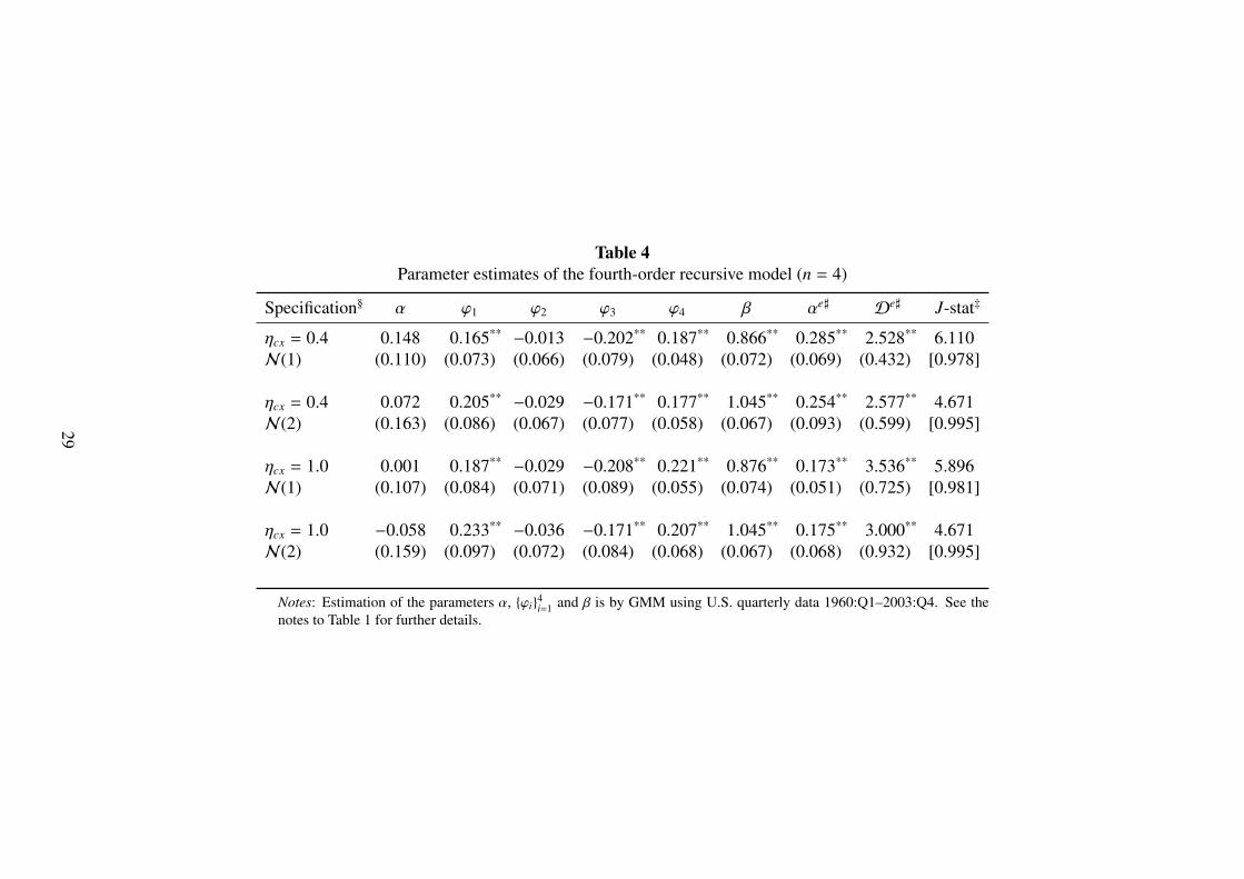
Table 4Parameter estimates of the fourth-order recursive model (n = 4)

Specification§ α ϕ1 ϕ2 ϕ3 ϕ4 β αe] De] J-stat‡

ηcx = 0.4 0.148 0.165** −0.013 −0.202** 0.187** 0.866** 0.285** 2.528** 6.110N(1) (0.110) (0.073) (0.066) (0.079) (0.048) (0.072) (0.069) (0.432) [0.978]

ηcx = 0.4 0.072 0.205** −0.029 −0.171** 0.177** 1.045** 0.254** 2.577** 4.671N(2) (0.163) (0.086) (0.067) (0.077) (0.058) (0.067) (0.093) (0.599) [0.995]

ηcx = 1.0 0.001 0.187** −0.029 −0.208** 0.221** 0.876** 0.173** 3.536** 5.896N(1) (0.107) (0.084) (0.071) (0.089) (0.055) (0.074) (0.051) (0.725) [0.981]

ηcx = 1.0 −0.058 0.233** −0.036 −0.171** 0.207** 1.045** 0.175** 3.000** 4.671N(2) (0.159) (0.097) (0.072) (0.084) (0.068) (0.067) (0.068) (0.932) [0.995]

Notes: Estimation of the parameters α, ϕi4i=1 and β is by GMM using U.S. quarterly data 1960:Q1–2003:Q4. See the

notes to Table 1 for further details.

29

Table 5Implied Phillips curve for the estimated fourth-order recursive model (n = 4)

Specification§ πt−1 πt−2 πt−3 πt−4 Etπt+1 Etπt+2 Etπt+3 Etπt+4 Etπt+5 xt

ηcx = 0.4 0.183** 0.008 −0.182** 0.222** 0.889** −0.136** −0.004 0.119** −0.108** 0.048*

N(1) (0.067) (0.065) (0.080) (0.058) (0.061) (0.058) (0.046) (0.058) (0.047) (0.028)

ηcx = 0.4 0.207** 0.012 −0.172** 0.184** 1.034** −0.228** −0.014 0.195** −0.229** 0.025N(2) (0.064) (0.070) (0.074) (0.057) (0.050) (0.071) (0.077) (0.091) (0.086) (0.023)

ηcx = 1.0 0.181** 0.005 −0.179** 0.220** 0.898** −0.138** −0.002 0.122** −0.114** 0.041N(1) (0.067) (0.065) (0.080) (0.058) (0.063) (0.059) (0.048) (0.060) (0.050) (0.027)

ηcx = 1.0 0.207** 0.012 −0.172** 0.184** 1.034** −0.228** −0.014 0.195** −0.229** 0.025N(2) (0.064) (0.070) (0.074) (0.057) (0.050) (0.071) (0.077) (0.091) (0.086) (0.023)

Notes: This table reports the coefficients of the Phillips curve (23) implied by the parameter estimates in Table 4 for each specification.Standard errors are given in parentheses and are calculated using the delta method. See the notes to Tables 1 and 4 for more detailsabout the estimation.

30

Figure 1Comparison of the hazard and survival functions implied by Examples 1 and 2

Hazard functions

Duration of price stickiness (i)

αi

Example 2

Survival functions

Duration of price stickiness (i)

ςi

Example 2

Example 1

Example 1

0 1 2 3 4 5 6 7 8 9 10 11 12

0 1 2 3 4 5 6 7 8 9 10 11 12

0

0.2

0.4

0.6

0.8

1

0

0.2

0.4

0.6

0.8

1

Notes: The hazard function sequences αi∞i=0 are generated by equation (7). Example 1 sets n = 0 and

α = 0.25; Example 2 uses n = 1, α = 0 and ϕ = 0.25. The corresponding survival function sequencesςi

∞i=0 are obtained from (8).

31

Figure 2Estimated hazard function and survival function for the Calvo pricing model (n = 0)

Hazard function

Quarters (i)

αi

Survival function

Quarters (i)

ςi

0 1 2 3 4 5 6 7 8 9 10

0 1 2 3 4 5 6 7 8 9 10

0

0.2

0.4

0.6

0.8

1

0

0.2

0.4

0.6

0.8

1

Notes: The hazard and survival functions are calculated from (7) and (8) using the estimated parametersfrom Table 1 under the preferred specification ηcx = 0.4 andN(1). In the graphs, the point estimate is shownas a cross in the middle of a darkly shaded thick bar that represents a one-standard-deviation band aroundthe point estimate, which is itself surrounded by a lightly shaded thin bar giving the two-standard-devationsband. The standard deviation is calculated using the delta method.

32

Figure 3Estimated hazard function and survival function for the first-order recursive model (n = 1)

Hazard function

Quarters (i)

αi

Survival function

Quarters (i)

ςi

0 1 2 3 4 5 6 7 8 9 10

0 1 2 3 4 5 6 7 8 9 10

0

0.2

0.4

0.6

0.8

1

0

0.2

0.4

0.6

0.8

1

Notes: The hazard and survival functions are calculated from (7) and (8) using the estimated parametersfrom Table 1 under the preferred specification ηcx = 0.4 andN(1). In the graphs, the point estimate is shownas a cross in the middle of a darkly shaded thick bar that represents a one-standard-deviation band aroundthe point estimate, which is itself surrounded by a lightly shaded thin bar giving the two-standard-devationsband. The standard deviation is calculated using the delta method.

33

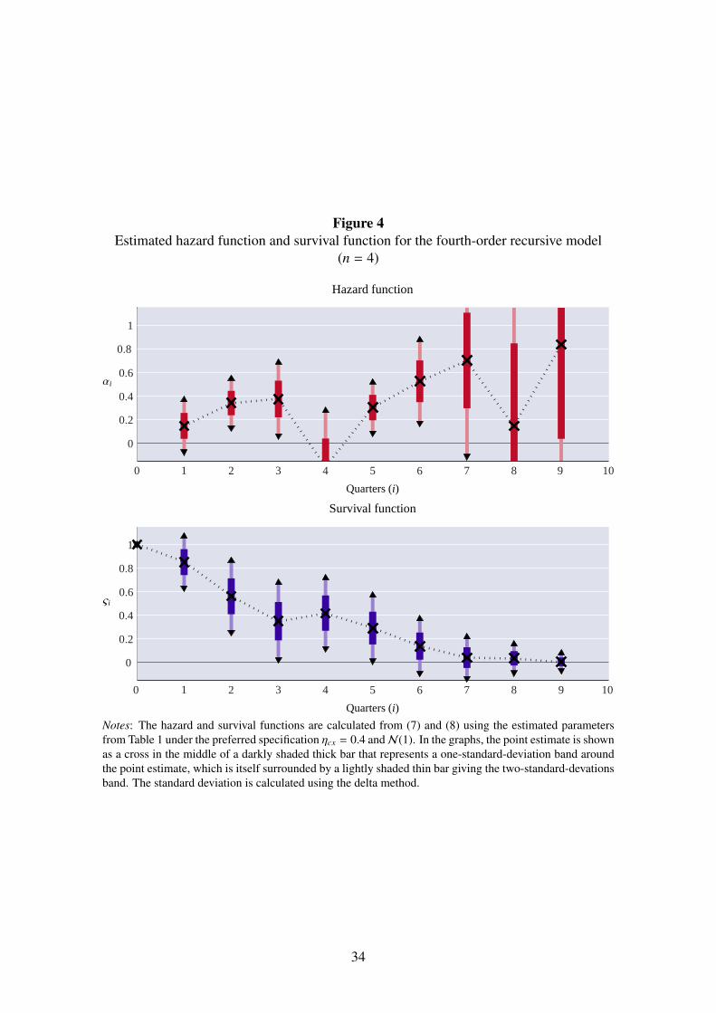
Figure 4Estimated hazard function and survival function for the fourth-order recursive model

(n = 4)

Hazard function

Quarters (i)

αi

Survival function

Quarters (i)

ςi

0 1 2 3 4 5 6 7 8 9 10

0 1 2 3 4 5 6 7 8 9 10

0

0.2

0.4

0.6

0.8

1

0

0.2

0.4

0.6

0.8

1

Notes: The hazard and survival functions are calculated from (7) and (8) using the estimated parametersfrom Table 1 under the preferred specification ηcx = 0.4 andN(1). In the graphs, the point estimate is shownas a cross in the middle of a darkly shaded thick bar that represents a one-standard-deviation band aroundthe point estimate, which is itself surrounded by a lightly shaded thin bar giving the two-standard-devationsband. The standard deviation is calculated using the delta method.

34

A. Technical appendix

A.1 Proof of Lemma 1

Let g be a number lying strictly between (1 − d) and 1, which must satisfy 0 < g < 1. Thedefinition of g then implies that ςi+1 ≤ gςi and hence ςi ≤ g

iς0 for all i ≥ 0. Now let x be anynumber strictly between 1 and g−1.

(i) The constant x is defined so that 1 < x < g−1 which implies 0 < gx < 1 and hence that∑∞i=0 g

i|z|i converges for all z in the disc Dx. By applying the triangle inequality to the functionς(z) it follows that |ς(z)| ≤ ς0/(1 − gx) if z ∈ Dx, and therefore that ς(z) is analytic on Dx.

(ii) Construct a new function G(z) ≡ (1 − gz)ς(z), which inherits the property that it isanalytic onDx from ς(z). Using the definition of ς(z), G(z) can be written as the sum of G0(z) ≡ς0 and G1(z) ≡ −

∑∞i=1(gςi−1 − ςi)zi. Now take any z ∈ Dx. Since |z|i ≤ xi and ςi ≤ gςi−1 the

triangle inequality and some algebraic manipulations show that |G1(z)| ≤ gxς0−∑∞

i=1(1−gx)xiςi.Because 0 < gx < 1 and |G0(z)| = ς0, it is established that |G1(z)| < |G0(z)| for all z ∈ Dx.

As a constant function, G0(z) must be analytic, and G1(z) inherits the property from G(z).Since G(z) = G0(z) + G1(z), Rouche’s Theorem implies that G(z) and G0(z) have the samenumber of zeros onDx.18 Since G0(z) clearly has no zeros on this set, neither has G(z). Becauseits definition ensures that G(z) inherits any roots of ς(z) = 0, this precludes ς(z) having a zeroin Dx as well.

A.2 Proof of Proposition 1

When deriving the following results, it is convenient to assume n = ∞ in (7) and set anysuperfluous ϕi parameters to zero.

(a) This follows immediately from equation (7) by induction.(b) i. Suppose that the first h recursive parameters are non-negative. Equation (7) then

clearly implies α2 ≥ α1. Now suppose that α1 ≤ α2 ≤ · · · ≤ αi−1 ≤ αi has already beenestablished for some i ≤ h. The slope of the hazard function can be obtained from (7):

αi+1 − αi =

i−1∑j=1

ϕ j(αi − αi− j)

i∏k=i− j

(1 − αk)

−1

+ ϕi

i∏k=1

(1 − αk)

−1

(A.1)

Given the initial supposition, the second term is unambiguously positive, and assuming thetruth of the induction step, the first term must be non-negative. Hence αi+1 ≥ αi, and so theclaim is proved by induction.

ii. Now suppose that αi+1 > αi, but ϕi ≤ 0 for all i = 1, . . . , h. By making use of (A.1)this leads to a contradiction, thus proving the claim.

iii. This follows from the result in part (c)i. below.

18I am indebted to Graham Brightwell for suggesting this use of Rouche’s Theorem. See any text on complexanalysis, such as Gamelin (2001), for further details about the theorem.

35

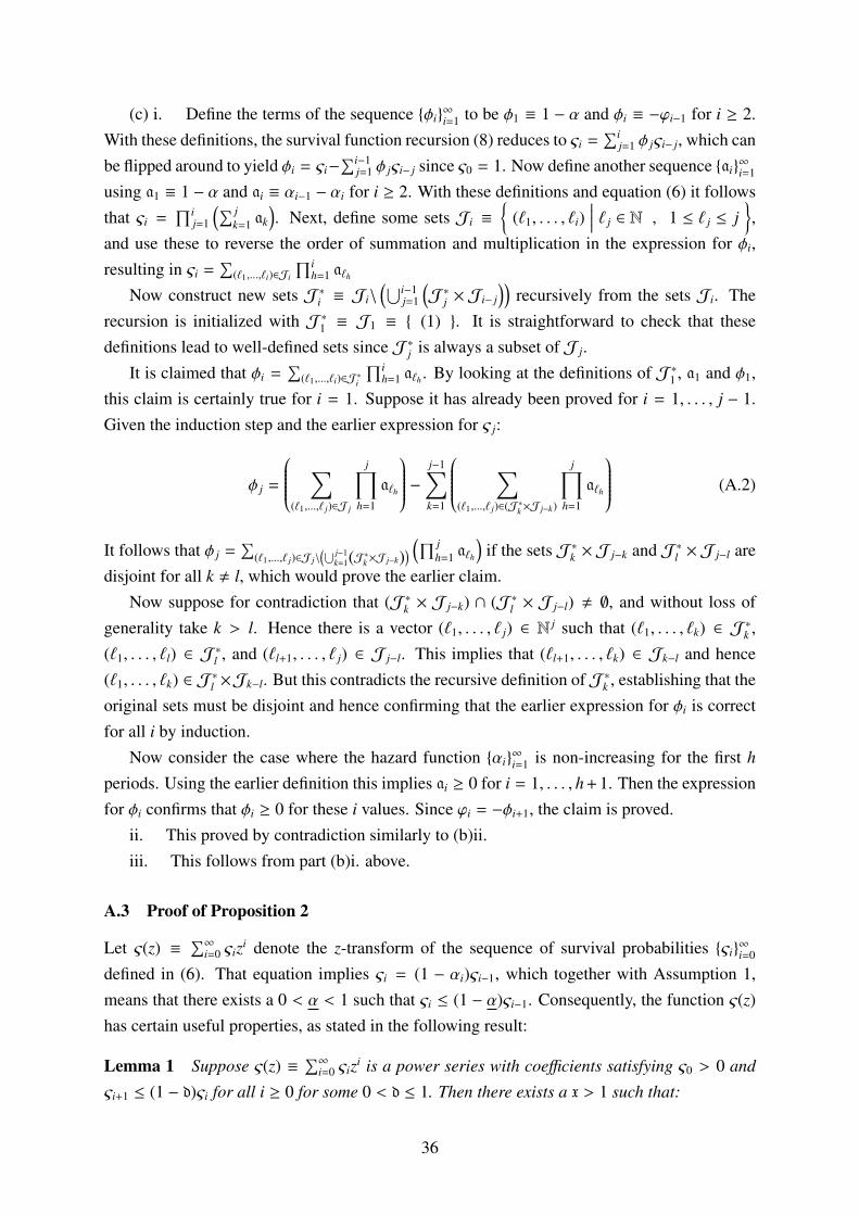
(c) i. Define the terms of the sequence φi∞i=1 to be φ1 ≡ 1 − α and φi ≡ −ϕi−1 for i ≥ 2.

With these definitions, the survival function recursion (8) reduces to ςi =∑i

j=1 φ jςi− j, which canbe flipped around to yield φi = ςi−

∑i−1j=1 φ jςi− j since ς0 = 1. Now define another sequence ai∞i=1

using a1 ≡ 1 − α and ai ≡ αi−1 − αi for i ≥ 2. With these definitions and equation (6) it followsthat ςi =

∏ij=1

(∑ jk=1 ak

). Next, define some sets Ji ≡

(`1, . . . , `i)

∣∣∣∣ ` j ∈ N , 1 ≤ ` j ≤ j,

and use these to reverse the order of summation and multiplication in the expression for φi,resulting in ςi =

∑(`1,...,`i)∈Ji

∏ih=1 a`h

Now construct new sets J∗i ≡ Ji\(⋃i−1

j=1

(J∗j × Ji− j

))recursively from the sets Ji. The

recursion is initialized with J∗1 ≡ J1 ≡ (1) . It is straightforward to check that thesedefinitions lead to well-defined sets since J∗j is always a subset of J j.

It is claimed that φi =∑

(`1,...,`i)∈J∗i

∏ih=1 a`h . By looking at the definitions of J∗1 , a1 and φ1,

this claim is certainly true for i = 1. Suppose it has already been proved for i = 1, . . . , j − 1.Given the induction step and the earlier expression for ς j:

φ j =

∑(`1,...,` j)∈J j

j∏h=1

a`h

− j−1∑k=1

∑(`1,...,` j)∈(J∗k×J j−k)

j∏h=1

a`h

(A.2)

It follows that φ j =∑

(`1,...,` j)∈J j\(⋃ j−1

k=1(J∗k×J j−k)) (∏ j

h=1 a`h

)if the sets J∗k × J j−k and J∗l × J j−l are

disjoint for all k , l, which would prove the earlier claim.Now suppose for contradiction that (J∗k × J j−k) ∩ (J∗l × J j−l) , ∅, and without loss of

generality take k > l. Hence there is a vector (`1, . . . , ` j) ∈ N j such that (`1, . . . , `k) ∈ J∗k ,(`1, . . . , `l) ∈ J∗l , and (`l+1, . . . , ` j) ∈ J j−l. This implies that (`l+1, . . . , `k) ∈ Jk−l and hence(`1, . . . , `k) ∈ J∗l ×Jk−l. But this contradicts the recursive definition ofJ∗k , establishing that theoriginal sets must be disjoint and hence confirming that the earlier expression for φi is correctfor all i by induction.

Now consider the case where the hazard function αi∞i=1 is non-increasing for the first h

periods. Using the earlier definition this implies ai ≥ 0 for i = 1, . . . , h + 1. Then the expressionfor φi confirms that φi ≥ 0 for these i values. Since ϕi = −φi+1, the claim is proved.

ii. This proved by contradiction similarly to (b)ii.iii. This follows from part (b)i. above.

A.3 Proof of Proposition 2

Let ς(z) ≡∑∞

i=0 ςizi denote the z-transform of the sequence of survival probabilities ςi∞i=0

defined in (6). That equation implies ςi = (1 − αi)ςi−1, which together with Assumption 1,means that there exists a 0 < α < 1 such that ςi ≤ (1 − α)ςi−1. Consequently, the function ς(z)has certain useful properties, as stated in the following result:

Lemma 1 Suppose ς(z) ≡∑∞

i=0 ςizi is a power series with coefficients satisfying ς0 > 0 and

ςi+1 ≤ (1 − d)ςi for all i ≥ 0 for some 0 < d ≤ 1. Then there exists a x > 1 such that:

36

(i) The power series ς(z) is convergent and analytic on the closed disc Dx ≡z ∈ C

∣∣∣ |z| ≤ xcentred at the origin with radius x.

(ii) The equation ς(z) = 0 has no roots in the set Dx.

Proof. See appendix A.1

Hence by setting d ≡ α, there must exist a x > 1 such that ς(z) is convergent, analytic andhas no zeros on Dx.

(i) Define the function φ(z) = 1/ς(z), which is well-defined and analytic because of theprevious result, and thus φ(z) can be written as a convergent power series for all z ∈ Dx. Itis always the case that ς0 = 1, so φ(0) = 1, and hence the power series can be expressed asφ(z) = 1−

∑∞i=1 φizi in terms of a sequence of coefficients φi

∞i=1. Since φ(z)ς(z) = 1, by equating

coefficients of powers of z it follows that φi = ςi −∑i−1

j=1 ς jφi− j, and by making the definitionsα ≡ 1−φ1 and ϕi ≡ −φi+1, the survival function recursion recursion (8) is obtained with n = ∞.This is equivalent to the hazard function recursion (7) when n = ∞.

(ii) Since φ(z) is analytic on Dx and x > 1 it must be the case that α +∑∞

i=1 ϕi < ∞, andhence ϕi → 0 as i→ ∞.

(iii) This is straightforward to prove by induction using (7).

A.4 Proof of Proposition 3

Assume ϕ , 0, since the case ϕ = 0 trivially requires just 0 < α < 1 for Assumption 1 tohold. Let φ(z) ≡ 1 − (1 − α)z + ϕz2 = (1 − ζ1z)(1 − ζ2z) be the characteristic polynomial forthe survival function recursion, where ζ1 and ζ2 denote the reciprocals of the roots of φ(z) = 0.These satisfy 1 − α = ζ1 + ζ2 and ϕ = ζ1ζ2.

Consider first the case where ϕ > 0. If αi satisfies 0 < αi ≤ α for some 0 < α < 1 then(7) implies 0 < αi+1 ≤ α + ϕ/(1 − α). It follows that a sufficient condition for Assumption 1 tobe satisfied is α ≥ α + ϕ/(1 − α) for some 0 < α < 1. This is equivalent to φ

((1 − α)−1

)≤ 0,

which requires that the quadratic equation φ(z) = 0 has real roots. The condition for this isϕ ≤ 1

4 (1 − α)2, which is one of the restrictions in (9).If ζ1 and ζ2 are real then when 0 < α < 1 and ϕ > 0 it follows that ζ1 > 0 and ζ2 > 0.

Without loss of generality, let ζ1 be the largest reciprocal root. Then it must be the case that0 < ζ1 < 1, and hence there is a α such that 0 < α < 1 and φ

((1 − α)−1

)≤ 0, guaranteeing that

Assumption 1 holds.Now consider the case ϕ < 0, where both roots are automatically real numbers. Here the

two roots must have opposite signs, and without loss of generality, suppose ζ1 > 0 and ζ2 < 0.Since 0 < α < 1, it must be the case that ζ1 > −ζ2. Suppose that (9) holds. Then it follows thatφ(z) > 0 for all 0 ≤ z ≤ 1, and because φ

(ζ−1

1

)= 0, it must be the case that ζ1 < 1.

Since ζ1 and ζ2 are distinct numbers, the survival function sequence ςi∞i=0 can be expressed

37

as ςi = c1ζi1 + c2ζ

i2, where c1 and c2 are real numbers, and in the following alternative forms:

ςi = c1ζi1

1 +c2

c1

(ζ2

ζ1

)i , ςi − ςi+1 = c1(1 − ζ1)ζ i

1

1 +c2(1 − ζ2)c1(1 − ζ1)

(ζ2

ζ1

)i (A.3)

From (7) it is seen that the first two terms of the hazard function are always α1 = α andα2 = α + ϕ/(1 − α). Since 0 < α < 1 and ϕ < 0, the second term is well defined if and only ifϕ > −α(1 − α) holds. Hence given (9), the survival function satisfies 0 ≤ ς2 < ς1 < ς0 = 1. Byusing (A.3), ς0 − ς1 = c1(1− ζ1) + c2(1− ζ2) > 0 and ς1 − ς2 = c1(1− ζ1)ζ1 + c2(1− ζ2)ζ2 > 0. Itfollows from these two inequalities that c1 > 0 and c1(1 − ζ1) > 0.

Because ζ1 > −ζ2, the terms (c2/c1)(ζ2/ζ1)i and (c2(1 − ζ2)/c1(1 − ζ1))(ζ2/ζ1)i must alternatein sign and decline in absolute value as i increases. Because c1, ζ1 and (1 − ζ1) are positive, theinequalities 0 ≤ ς2 < ς1 < ς0 imply 0 ≤ ςi < ςi−1 for all i ≥ 1, guaranteeing that Assumption 1holds.

To see the converse, suppose Assumption 1 is true. As the first two terms of the hazardfunction are well defined, the part of (9) for ϕ < 0 must hold. And since the survival functionsequence cannot feature oscillations, this requires that the roots of φ(z) = 0 are real numbers,implying the second part of (9) for ϕ > 0.

A.5 Proof of Proposition 4

Let T (·) be the mapping from a distribution at time t to the distribution at time t + 1 implied by(15), that is, θi,t+1

∞i=0 = T

(θit

∞i=0

). Define m ≡ min

i∣∣∣ αi+1 = 1

to be the maximum duration

of price stickiness implied by the hazard function, noting that the case of m = ∞ is possible.Attention can be restricted to the set Sm ≡

θi

mi=0

∣∣∣∣ 0 ≤ θi ≤ 1 ,∑m

i=0 θi = 1

of probabilitydistributions for the duration of price stickiness up to a maximum of m periods. Let Tm(·) bethe corresponding mapping from Sm to Sm defined by equation (15).

(i) Under Assumption 1, Lemma 1 can be applied to the z-transform ς(z) ≡∑∞

i=0 ςizi ofthe survival probabilities ςi

∞i=0. It follows that

∑∞i=0 ςi is finite. Define a distribution θi

∞i=0

using θi ≡ ςi/∑∞

j=0 ς j. This is a well-defined probability distribution, and equations (6) and(15) imply that it is a fixed point of Tm(·).

Define Vm ≡

vi

mi=0

∣∣∣∣ vimi=0 = ϑi

mi=0 − θi

mi=0 , ϑi

mi=0 ∈ Sm

to be the set of possible

deviations from the first m + 1 terms of the stationary distribution θi∞i=0. It is straightforward

to see that Vm is a subset of the linear space Wm ≡

vi

mi=0

∣∣∣∣ ∑mi=0 vi = 0

. The definition of

Tm(·) in (15) shows that it can also be seen as a linear transformation fromWm toWm.An eigenvalue of Tm : Wm → Wm is a scalar ζ ∈ C such there is a non-zero sequence

vimi=0 ∈ Wm and Tm

(vi

mi=0

)= ζvi

mi=0. This sequence is referred to as an eigenvector. Equa-

tion (15) shows that any eigenvalue and eigenvector pair must satisfy∑m+1

i=1 αivi−1 = ζv0 and(1 − αi)vi−1 = ζvi for all i = 1, . . . ,m. As the definition of the maximum duration of pricestickiness m guarantees that αi < 1 for all i ≤ m, it must be the case that ζ , 0, other-

38

wise the sequence vimi=0 could not be an eigenvector. It follows that vi = ςiv0/ζ

i and hence∑mi=0 ςi/ζ

i = 0, or equivalently ς(ζ−1

)= 0. Because ς(z) has no zeros in Dx and x > 1, all

the eigenvalues of Tm lie strictly inside the unit circle. Therefore, the stationary distribution isunique and the economy must converge to it starting from any initial conditions.

(ii) Define φ(z) ≡ 1 − (1 − α)z +∑n

i=1 ϕizi+1 to be the characteristic polynomial for thesurvival function recursion in (8). The functions φ(z) is then related to ς(z) by φ(z)ς(z) = 1.The definition of the stationary distribution implies θi = ςi/ς(1), but then ς(1) = 1/φ(1) andφ(1) = α +

∑nj=1 ϕ j, thus confirming the first part of (16).

The unconditional expectation of the probability of price adjustment is αe ≡∑∞

i=1 αiθi−1.The previous result combined with (6) implies αi = 1−(θi/θi−1), and so αe =

∑∞i=0(θi−θi+1) = θ0,

and since θ0 =(α +

∑ni=1 ϕi

)ς0, the second part of (16) is shown to be correct.

The unconditional expectation of the duration of price stickiness is De ≡∑∞

i=1 iθi−1. Letθ(z) ≡

∑∞i=0 θizi be the z-transform of the sequence θi

∞i=0, which is analytic on Dx because of

the properties of ς(z). Therefore the power series can be differentiated term-by-term to yieldθ′(z) =

∑∞i=0 iθizi−1. It is then seen thatDe = θ′(1) + θ(1). Since θ(z) = φ(1)/φ(z), it follows that

θ′(z) = −φ(1)φ′(z)/(φ(z))2 and hence De = (φ(1) − φ′(1))/φ(1). The definition of φ(z) yieldsφ′(z) = −(1 − α) +

∑ni=1(i + 1)ϕizi, proving the third part of (16).

A.6 Proof of Theorem 1

Define the sequence φin+1i=1 with φ1 ≡ 1−α and φi = −ϕi−1 for i ≥ 2, and set φ(z) ≡ 1−

∑n+1i=1 φizi.

Then let ς(z) ≡∑∞

i=0 ςizi and θ(z) ≡∑∞

i=0 θizi be the z-transforms of the survival function and theduration distribution respectively. As Assumption 1 holds, Lemma 1 and equation (8) implythat φ(z)ς(z) = 1 for all z in the unit disc D. It then follows from equation (16) of Proposition4 that φ(z)θ(z) = φ(1) for all z ∈ D. In terms of the lag operator and the forward operator ,the equations in (19) can be expressed as Rt = t[(ς(β)/ς(β))(Pt + ηcxxt)] and Pt = θ()Rt.The equivalent recursive versions in (20) and (22) are t[φ(β)Rt] = φ(β)(Pt + ηcxxt) andφ()Pt = φ(1)Rt.

By substituting the recursive equation for the reset price into the recursive equation for theprice level, the stochastic difference equation t[Υ()Pt] = fηcxxt is obtained with definitionsΥ(z) ≡ φ(z)φ(βz−1) − φ(1)φ(β) and f ≡ φ(1)φ(β). The function Υ(z) has the symmetry propertyΥ(z) = Υ(βz−1) for all z , 0. Together with the definition of φ(z) this implies that Υ(z) can bewritten as Υ(z) ≡ Υ0 +

∑n+1i=1 Υi

(zi + βiz−i

)with Υi = −

(φi −

∑n+1−ij=1 β jφ jφi+ j

)for i ≥ 1.

The definition of Υ(z) ensures that Υ(1) = 0. It follows that there exists a function ψ(z) ≡1 −

∑ni=1 ψizi −

∑n+1i=1 δiz−i and a constant κ such that Υ(z) = (f/κ)(1 − z)ψ(z). This allows

the stochastic difference equation involving prices and real marginal cost to be replaced by anequation t[ψ()πt] = κηcxxt in terms of inflation and real marginal cost. If this equation iswritten out in full and κx ≡ κηcx is defined then the Phillips curve given in (23) is obtained.

Expressions for the coefficients of the Phillips curve in terms of the hazard function para-

39

meters are obtained by using the relationship between the Υ(z) and ψ(z) functions and theexpression derived for Υi. The coefficients on lagged inflation are given by the expression ψi =

−(κ/f)∑n+1

j=i+1 φ j

(1 −

∑ j−(i+1)k=1 βkφk

). Similarly, the coefficients on inflation expectations and real

marginal cost are δi+1 = (κ/f)∑n+1

j=i+1 βjφ j

(1 −

∑ j−(i+1)k=1 φk

)and κ = f/

(∑n+1j=1 φ j

(1 −

∑ j−1k=1 β

kφk

))respectively. By using the definitions made at the beginning of this proof, all the coefficientscan be stated in terms of α, ϕi

ni=1, β and ηcx:

ψi =ϕi +

∑nj=i+1 ϕ j

(1 − β(1 − α) +

∑ j−1k=1 β

k+1ϕk

)(1 − α) −

∑nj=1 ϕ j

(1 − β(1 − α) +

∑ j−1k=1 β

k+1ϕk

) i = 1, . . . , n (A.4a)

δi+1 = −βi+1ϕi +

∑nj=i+1 β

j−iϕ j

(α +

∑ j−1k=1 ϕk

)(1 − α) −

∑nj=1 ϕ j

(1 − β(1 − α) +

∑ j−1k=1 β

k+1ϕk

) i = 1, . . . , n (A.4b)

δ1 = β(1 − α) −

∑nj=1 β

jϕ j

(α +

∑ j−1k=1 ϕk

)(1 − α) −

∑nj=1 ϕ j

(1 − β(1 − α) +

∑ j−1k=1 β

k+1ϕk

) (A.4c)

κx =ηcx

(α +

∑nj=1 ϕ j

) (1 − β(1 − α) +

∑nj=1 β

j+1ϕ j

)(1 − α) −

∑nj=1 ϕ j

(1 − β(1 − α) +

∑ j−1k=1 β

k+1ϕk

) (A.4d)

To establish the link between the signs of the sequences ϕini=1 and ψi

ni=1, note φ(z)ς(z) = 1,

0 < β < 1 and Assumption 1 imply 0 < α +∑n

i=1 ϕi < 1 and 0 < 1 − β(1 − α) +∑n

i=1 βi+1ϕi < 1.

(a) This follows immediately from (A.4a) by induction.(b) i. Consider the case where ϕi ≥ 0 for all i = 1, . . . , n. Since Assumption 1 requires

that 0 < α < 1, the inequalities stated above can be extended to yield 0 < α +∑ j−1

k=1 ϕk < 1 and0 < 1 − β(1 − α) +

∑ j−1k=1 β

k+1ϕk < 1 for all j = 1, . . . , n + 1. Therefore, by using the expressionfor ψi in (A.4a), ϕi ≥ 0 for all i = 1, . . . , n implies ψi ≥ 0 for i = 1, . . . , n. Similarly, ϕi > 0 forall i yields ψi > 0 for all i.

ii. The inequalities derived in part (b)i. also hold. The result follows immediately from(A.4a).

iii. This is the contrapositive of the claim proved in (c)i. below.(c) i. Now suppose ϕi ≤ 0 for all i = 1, . . . , n. Using similar reasoning to part (b)i. above,

the inequalities derived there must hold for all j = 1, . . . , n + 1. Hence from (A.4a), ϕi ≤ 0 forall i = 1, . . . , n implies ψi ≤ 0 for i = 1, . . . , n. In addition, ϕi < 0 for all i leads to ψi < 0 for alli.

ii. The inequalities derived in part (b)i. also hold, and the result follows from (A.4a).iii. This is the contrapositive of part (b)i. above, which has already been proved.

40

References

Altissimo, F., Bilke, L., Levin, A., Matha, T. and Mojon, B. (2006), ‘Sectoral and aggregateinflation dynamics in the euro area’, Journal of the European Economic Association, 4(2–3),pp. 585–593.

Alvarez, L. J., Burriel, P. and Hernando, I. (2005), ‘Do decreasing hazard functions for pricechanges make any sense?’, Working paper 461, European Central Bank.

Baumgartner, J., Glatzer, E., Rumler, F. and Stiglbauer, A. (2005), ‘How frequently do con-sumer prices change in Austria? Evidence from micro CPI data’, Working paper 523,European Central Bank.

Calvo, G. A. (1983), ‘Staggered prices in a utility-maximizing framework’, Journal ofMonetary Economics, 12, pp. 383–398.

Campbell, J. R. and Eden, B. (2005), ‘Rigid prices: Evidence from U.S. scanner data’, Workingpaper, Vanderbilt University.

Cecchetti, S. G. (1986), ‘The frequency of price adjustment: A study of the newsstand pricesof magazines’, Journal of Econometrics, 31, pp. 255–274.

Christiano, L. J., Eichenbaum, M. J. and Evans, C. L. (2005), ‘Nominal rigidities and thedynamic effects of a shock to monetary policy’, Journal of Political Economy, 113, pp. 1–45.

Cliff, M. T. (2003), ‘GMM and MINZ program libraries for MATLAB’, Working paper, Vir-ginia Tech, available for download from mcliff.cob.vt.edu/progs.html.

Cogley, T. and Sbordone, A. M. (2005), ‘A search for a structural Phillips curve’, Staff report203, Federal Reserve Bank of New York.

Dias, D. A., Marques, C. R. and Santos Silva, J. M. C. (2005), ‘Time or state dependent pricesetting rules? Evidence from Portuguese micro data’, Working paper 511, European CentralBank.

Dittmar, R. D., Gavin, W. T. and Kydland, F. E. (2005), ‘Inflation persistence and flexibleprices’, International Economic Review, 46(1), pp. 245–261.

Dotsey, M. (2002), ‘Pitfalls in interpreting tests of backward-looking pricing in New Keynesianmodels’, Federal Reserve Bank of Richmond Economic Quarterly, 88, pp. 37–50.

Dotsey, M., King, R. G. and Wolman, A. L. (1999), ‘State dependent pricing and the generalequilibrium dynamics of money and output’, Quarterly Journal of Economics, 114(2), pp.655–690.

41

Fougere, D., Le Bihan, H. and Sevestre, P. (2005), ‘Heterogeneity in consumer price stickiness:A microeconometric investigation’, Working paper 536, European Central Bank.

Fuhrer, J. C. (1997), ‘The (un)importance of forward-looking behavior in price specifications’,Journal of Money, Credit and Banking, 29, pp. 338–350.

Fuhrer, J. C. and Moore, G. R. (1995), ‘Inflation persistence’, Quarterly Journal of Economics,109, pp. 197–230.

Gadzinski, G. and Orlandi, F. (2004), ‘Inflation persistence in the European Union, the EuroArea, and the United States’, Working paper 414, European Central Bank.

Galı, J. and Gertler, M. (1999), ‘Inflation dynamics: A structural econometric analysis’, Journalof Monetary Economics, 44, pp. 195–222.

Galı, J., Gertler, M. and Lopez-Salido, J. D. (2001), ‘European inflation dynamics’, EuropeanEconomic Review, 45, pp. 1237–1270.

Gamelin, T. W. (2001), Complex Analysis, Springer-Verlag, New York.

Goodfriend, M. and King, R. G. (1997), ‘The New Neoclassical synthesis and the role of mon-etary policy’, NBER Macroeconomics Annual, 12, pp. 231–283.

Gotte, L., Minsch, R. and Tyran, J.-R. (2005), ‘Micro evidence on the adjustment of sticky-price goods: It’s how often, not how much’, Discussion paper 5364, Centre for EconomicPolicy Research.

Guerrieri, L. (2001), ‘Inflation dynamics’, International finance discussion paper 715, FederalReserve Board.

Guerrieri, L. (2002), ‘The inflation persistence of staggered contracts’, International financediscussion paper 734, Federal Reserve Board.

Heckman, J. and Singer, B. (1984), ‘Econometric duration analysis’, Journal of Econometrics,24, pp. 63–132.

Jadresic, E. (1999), ‘Sticky prices: An empirical assessment of alternative models’, Workingpaper 99/72, International Monetary Fund.

Kiefer, N. (1988), ‘Economic duration data and hazard functions’, Journal of EconomicLiterature, 26, pp. 646–679.

Kurmann, A. (2004), ‘Maximum likelihood estimation of dynamic stochastic theories withan application to New Keynesian pricing’, Working paper 04–21, Universite du Quebec aMontreal.

42

Linde, J. (2005), ‘Estimating New-Keynesian Phillips curves: A full information maximumlikelihood approach’, Journal of Monetary Economics, 52(6), pp. 1135–1149.

Mankiw, N. G. (2001), ‘The inexorable and mysterious trade-off between inflation and unem-ployment’, Economic Journal, 111, pp. C45–61.

Mash, R. (2004), ‘Optimizing microfoundations for inflation persistence’, Discussion paper183, Oxford University.

Matyas, L. (1999), Generalized Method of Moments Estimation, Cambridge University Press,Cambridge.

Milani, F. (2005), ‘Adaptive learning and inflation persistence’, Working paper, Princeton Uni-versity.

Nakamura, E. and Steinsson, J. (2007), ‘Five facts about prices: A reevaluation of menu costmodels’, Working paper, Harvard University.

Paloviita, M. (2004), ‘Inflation dynamics in the euro area and the role of expectations: Furtherresults’, Discussion paper 21, Bank of Finland.

Roberts, J. M. (1997), ‘Is inflation sticky?’, Journal of Monetary Economics, 39, pp. 173–196.

Roberts, J. M. (2005), ‘How well does the New Keynesian sticky-price model fit the data?’,Contributions to Macroeconomics, 5(1), p. Article 10.

Rudd, J. and Whelan, K. (2005), ‘New tests of the New-Keynesian Phillips curve’, Journal ofMonetary Economics, 52(6), pp. 1167–1181.

Sbordone, A. (2002), ‘Prices and unit labor costs: A new test of price stickiness’, Journal ofMonetary Economics, 49, pp. 235–256.

Sheedy, K. D. (2007), ‘Robustly optimal monetary policy’, Working paper, London School ofEconomics.

Smets, F. and Wouters, R. (2003), ‘An estimated dynamic stochastic general equilibrium modelof the euro area’, Journal of the European Economic Association, 1(5), pp. 1123–1175.

Taylor, J. B. (1980), ‘Aggregate dynamics and staggered contracts’, Journal of PoliticalEconomy, 88, pp. 1–24.

Whelan, K. (2007), ‘Staggered price contracts and inflation persistence: Some general results’,International Economic Review, 48(1), pp. 111–145.

Wolman, A. L. (1999), ‘Sticky prices, marginal cost, and the behavior of inflation’, FederalReserve Bank of Richmond Economic Quarterly, 85(4), pp. 29–48.

43

Woodford, M. (2003), Interest and Prices: Foundations of a Theory of Monetary Policy, Prin-ceton University Press, New Jersey.

Woodford, M. (2007), ‘Interpreting inflation persistence: Comments on the conference on‘Quantitative Evidence on Price Determination’’, Journal of Money, Credit and Banking,39(1), pp. 203–210.

44

CENTRE FOR ECONOMIC PERFORMANCE Recent Discussion Papers

836 Andrew E. Clark Ed Diener Yannis Georgellis Richard E. Lucas

Lags and Leads in Life Satisfaction: A Test of the Baseline Hypothesis

835 Jean-Baptiste Michau Creative Destruction with On-the-Job Search

834 Nikolaus Wolf Scylla and Charybodis: the European Economy and Poland's Adherence to Gold, 1928-1936

833 Sharon Belenzon Tomer Berkovitz

Innovation in Business Groups

832 Espen R. Moen Åsa Rosén

Incentives in Competitive Search Equilibrium

831 Eran Yashiv U.S. Labor Market Dynamics Revisited

830 Laura Alfaro Andrew Charlton

Growth and the Quality of Foreign Direct Investment: Is All FDI Equal?

829 Richard Layard David Clark Martin Knapp Guy Mayraz

Cost-Benefit Analysis of Psychological Therapy

828 Emma Tominey Maternal Smoking During Pregnancy and Early Child Outcomes

827 Christos Genakos Tommaso Valletti

Testing the “Waterbed” Effect in Mobile Telephony

826 Luis Garicano Paul Heaton

Information Technology, Organization, and Productivity in the Public Sector: Evidence from Police Departments

825 Laura Alfaro Andrew Charlton

Intra-Industry Foreign Direct Investment

824 Miklós Koren Silvana Tenreyro

Technological Diversification

823 Régis Barnichon The Shimer Puzzle and the Correct Identification of Productivity Shocks

822 Carlos Thomas Search Frictions, Real Rigidities and Inflation Dynamics

821 Giulia Faggio Kjell G. Salvanes John Van Reenen

The Evolution of Inequality in Productivity and Wages: Panel Data Evidence

820 Luis Araujo Emanuel Ornelas

Trust-Based Trade

819 Régis Barnichon Productivity, Aggregate Demand and Unemployment Fluctuations

818 Rachel Griffith Sokbae Lee John Van Reenen

Is Distance Dying at Last? Falling Home Bias in Fixed Effects Models of Patent Citations

817 Tsutomu Miyagawa YoungGak Kim

Measuring Organization Capital in Japan: An Empirical Assessment Using Firm-Level Data

816 Andreas Georgiadis Alan Manning

Spend It Like Beckham? Inequality and Redistribution in the UK, 1983-2004

815 Guy Michaels Xiaojia Zhi

Freedom Fries

814 Ralph Ossa Trade Liberalization, Outsourcing, and Firm Productivity

813 Karsten Kohn Alexander C. Lembcke

Wage Distributions by Bargaining Regime: Linked Employer-Employee Data Evidence from Germany

812 Yannis M. Ioannides Henry G. Overman Esteban Rossi-Hansberg Kurt Schmidheiny

The Effect of Information and Communication Technologies on Urban Structure

811 Guy Michaels The Division of Labor, Coordination, and the Demand for Information Processing

810 Maia Güell Jose V. Rodriguez Mora Chris Telmer

Intergenerational Mobility and the Informative Content of Surnames

809 Stephen J. Redding Daniel M. Sturm Nikolaus Wolf

History and Industry Location: Evidence from German Airports

808 Anna Lipinska The Maastricht Convergence Criteria and Optimal Monetary Policy for the EMU Accession Countries

807 Eran Yashiv The Beveridge Curve

The Centre for Economic Performance Publications Unit Tel 020 7955 7673 Fax 020 7955 7595 Email info@cep.lse.ac.uk

Web site http://cep.lse.ac.uk