Macroeconomic Changes with

Declining Trend Inflation:

Complementarity with

the Superstar Firm Hypothesis

Takushi Kurozumi* takushi.kurozumi@boj.or.jp

Willem Van Zandweghe**

willem.vanzandweghe@clev.frb.org

No.21-E-13

November 2021

Bank of Japan

2-1-1 Nihonbashi-Hongokucho, Chuo-ku, Tokyo 103-0021, Japan

* Monetary Affairs Department, Bank of Japan ** Research Department, Federal Reserve Bank of Cleveland

Papers in the Bank of Japan Working Paper Series are circulated in order to stimulate discussion

and comments. Views expressed are those of authors and do not necessarily reflect those of

the Bank of Japan, the Federal Reserve Bank of Cleveland, or the Federal Reserve System.

If you have any comment or question on the working paper series, please contact each author.

When making a copy or reproduction of the content for commercial purposes, please contact the

Public Relations Department (post.prd8@boj.or.jp) at the Bank of Japan in advance to request

permission. When making a copy or reproduction, the source, Bank of Japan Working Paper

Series, should explicitly be credited.

Bank of Japan Working Paper Series

Macroeconomic Changes with Declining Trend Inflation:

Complementarity with the Superstar Firm Hypothesis∗

Takushi Kurozumi† Willem Van Zandweghe‡

Abstract

Recent studies indicate that, since 1980, the US economy has undergone increases

in the average markup and the profit share of income and decreases in the labor share

and the investment share of spending. We examine the role of monetary policy in these

changes as inflation has concurrently trended down. In a simple staggered price model

with a non-CES aggregator of individual differentiated goods, a decline of trend inflation

as measured since 1980 can account for a substantial portion of the changes. Moreover,

adding a rise of highly productive “superstar firms” to the model can better explain

not only the macroeconomic changes but also the micro evidence on the distribution of

firms’ markups, including the flat median markup.

JEL Classification: E52, L16

Keywords: Average markup; Profit share; Labor share; Trend inflation; Non-CES ag-

gregator; Superstar firm hypothesis

∗The authors are grateful to David Berger, Florin Bilbiie, Munechika Katayama, Koji Nakamura, BrentNeiman, Makoto Nirei, Vincenzo Quadrini, Richard Rogerson, Nao Sudo, and seminar participants at theFederal Reserve Bank of Cleveland and Waseda University for comments and discussions. The authors alsothank Todd Clark and Raphael Schoenle for sharing the data on the trend inflation rate and the frequencyof price adjustment, respectively, with us. Kristen Tauber provided excellent research assistance. The viewsexpressed in the paper are those of the authors and do not necessarily reflect the official views of the Bankof Japan, the Federal Reserve Bank of Cleveland, or the Federal Reserve System.†Monetary Affairs Department, Bank of Japan, 2-1-1 Nihonbashi-Hongokucho, Chuo-ku, Tokyo 103-8660,

Japan (e-mail: takushi.kurozumi@boj.or.jp)‡Research Department, Federal Reserve Bank of Cleveland, 1455 E 6th St, Cleveland, OH 44114, USA

(e-mail: willem.vanzandweghe@clev.frb.org)

1

1 Introduction

Recent studies have documented profound changes to the US economy since 1980. The

average price–cost markup has increased, as illustrated by the solid line in panel (a) of

Figure 1.1 Concurrently, the profit share of income has increased, while the labor share (of

income) and the investment share of spending have decreased, as shown by the solid lines

in panels (b), (c), and (d) of the figure, respectively.2 In each of the four panels a trend is

plotted by the dashed regression line, whose slope is significantly different from zero.

A growing literature has studied possible linkages between the US macroeconomic changes.

Barkai (2020) analyzes the link between the increase in the average markup and the decrease

in the labor share using aggregate data, and shows that the decrease has been more than

offset by a rise in pure profits, thus suggesting that the decreasing labor share is due to

a decline in competition.3 Autor et al. (2020) use micro panel data to address the link,

and find evidence consistent with a rise since the early 1980s of highly productive “superstar

firms,” which have increased concentration and markups and reduced the labor share in their

industries.4 In this context, De Loecker et al. (2020) investigate firm-level data and indicate

that the increase in the average markup is driven mainly by the upper tail of the distribu-

tion of firms’ markups. The link between higher markups and the lower investment share is

investigated by Covarrubias et al. (2020), who document a decrease in business investment

during the last two decades and attribute it to a rise in concentration and a decline in compe-

1Our measure of the average markup is the sales-weighted harmonic average markup, which coincides withthe cost-weighted arithmetic average markup. De Loecker et al. (2020) employ the sales-weighted arithmeticaverage markup as displayed in their Figure I, and point out that such an average markup measure exhibitsa larger increase, to 1.6 in 2016, because firms with higher markups tend to have higher sales weights relativeto their cost weights. Edmond et al. (2021) indicate that the cost-weighted arithmetic average markup is therelevant statistic that summarizes the distortions to employment and investment decisions, and they showan average markup series similar to ours.

2Akcigit and Ates (2021) highlight 10 facts on declining business dynamism in the US since 1980, includingthe increases in the average markup and the profit share and the decrease in the labor share.

3Barkai (2020) calculates that the profit share of income rose by 13.5 percentage points during the period1984–2014, a larger rise than that seen in panel (b) of Figure 1 (i.e., 7.5 percentage points during the sameperiod). Karabarbounis and Neiman (2019) cast doubt on the rising profit share.

4See also Elsby et al. (2013), Karabarbounis and Neiman (2014), and Kehrig and Vincent (2021) foranalyses of the decreasing labor share. Aum and Shin (2020) note that the decline in the labor shareaccelerated after 2000, and point to increased capital–labor substitution in the services sector as a possiblefactor behind the acceleration.

2

Figure 1: Evolution of key US macroeconomic variables.

1980 1990 2000 2010 20201.12

1.18

1.24

1.3

1.36(a) Average markup

1980 1990 2000 2010 20200

4

8

12

16

% o

f out

put

(b) Profit income

1980 1990 2000 2010 2020

Year

55

58

61

64

67

% o

f out

put

(c) Labor income

1980 1990 2000 2010 2020

Year

15

17

19

21

23

% o

f out

put

(d) Investment spending

Notes: In the figure the solid lines illustrate key US macroeconomic time series from 1980 to 2019 or themost recent available year and the dashed lines display their respective regression trends. Panel (a) shows thesales-weighted harmonic average markup, which coincides with the cost-weighted arithmetic average markup.Panel (b) exhibits corporate profits adjusted for inventory valuation and capital consumption as a share ofvalue added of the nonfinancial corporate sector. Panel (c) plots the labor share in the nonfarm businesssector. Panel (d) presents the share of business fixed investment in spending, where spending is measuredas the sum of business fixed investment, personal consumption expenditures (PCE) for nondurable goods,and PCE for services.Sources: De Loecker et al. (2020), US Bureau of Labor Statistics, US Bureau of Economic Analysis, HaverAnalytics.

3

tition.5 As for the forces driving some of the US macroeconomic changes, the literature has

pointed to globalization and technological changes (Autor et al., 2020), weakened antitrust

enforcement (Gutiérrez and Philippon, 2017), and patent concentration (Akcigit and Ates,

2021).

This paper examines the role of monetary policy as a driving factor behind the US

macroeconomic changes. In tandem with the changes, Figure 2 shows that inflation has

steadily trended down since 1980, a trend that is well-known but has hitherto not been linked

to the changes illustrated in Figure 1. The dashed line in Figure 2 displays the estimated

trend inflation series of Chan et al. (2018).6 The series of the (trend) inflation rate and

the average markup exhibit a negative association, suggesting the possibility of a structural

relationship between the two macroeconomic variables.7 Under lower trend inflation, firms’

price–cost markups are less severely eroded in between infrequent price adjustments, which

may raise the average markup. To see some empirical support for this, we conduct an

industry-level regression analysis of the change in the average markup from 1980 to 2016 on

the frequency of price adjustment, and find evidence that the change in the average markup

under the concurrent decline in trend inflation was larger for industries that adjust prices

less frequently.

To investigate the implications of declining trend inflation for the increasing average

markup and the three other macroeconomic changes, we use a simple staggered price model.8

A key feature of the model is that, each period, a fraction of individual goods’ prices re-

mains unchanged in line with micro evidence, while the other prices are set given demand

curves arising from a not necessarily constant elasticity of substitution (CES) aggregator

of individual differentiated goods of the sort proposed by Kimball (1995) and developed by

5Basu (2019) and Syverson (2019) provide excellent reviews of related studies.6See, e.g., Ireland (2007), Cogley and Sbordone (2008), and Ascari and Sbordone (2014) for alternative

estimates of trend inflation. The estimated series of Chan et al. (2018) exhibits a decline similar to those ofthe previous studies.

7The negative association between inflation and markups is consistent with the findings of empiricalstudies, such as Bénabou (1992) and Banerjee and Russell (2001, 2005).

8One may wonder how our paper treats the natural rate hypothesis. Despite the widely held view goingback to Friedman (1968), the empirical evidence on whether monetary policy has long-run real effects is notas clear-cut. Various recent empirical research has supported the notion that monetary policy can have long-lasting real effects. For example, Moran and Queralto (2018) demonstrate increases in R&D and medium-runTFP following an expansionary monetary policy shock. Jordà et al. (2020) show that the effects of monetarypolicy on TFP, capital accumulation, and the production capacity of the economy are long lived.

4

Figure 2: Evolution of US inflation.

1980 1990 2000 2010 2020

Year

-3

0

3

6

9

12

%

Notes: In the figure the solid and the dashed lines display the inflation rate of the personal consumptionexpenditures price index and its estimated trend of Chan et al. (2018) from 1980 to 2019, respectively.Sources: Chan et al. (2018), US Bureau of Economic Analysis, Haver Analytics.

Dotsey and King (2005) and Levin et al. (2008), which includes the CES aggregator as a

special case. The non-CES aggregator provides a parsimonious way of introducing variable

price elasticity of demand and hence endogenous desired markups of firms. Specifically, for a

lower (higher) relative price of a good, the price elasticity of demand for the good decreases

(increases), which raises (reduces) the firm’s desired markup and thus inhibits the firm from

setting such a relative price.9

The calibrated model shows that a decline of trend inflation as measured since 1980 can

account for a substantial portion of the US macroeconomic changes. The model attributes

around 30% of the increases in the average markup and the profit share and the decrease

in the labor share and about 20% of the decrease in the investment share to the decline in

trend inflation. The endogenous desired markups arising from the non-CES aggregator make

price-adjusting firms’ markups less responsive to trend inflation, because a lower relative price

induced by a decline in trend inflation raises the firms’ desired markups. At the same time,

the decline in trend inflation leads non-adjusting firms to experience a less severe erosion

9Because of this feature, the non-CES aggregator has been widely used as a source of real rigidity in themacroeconomic literature. See, e.g., Eichenbaum and Fisher (2007), Smets and Wouters (2007), Gopinathand Itskhoki (2011), and Kurozumi and Van Zandweghe (2016).

5

of their markups. This increases the average markup, which in turn raises the profit share

and reduces the labor share and the investment share in the model. This result contrasts

with that in the case of the CES aggregator in which the average markup is almost flat

for the decline in trend inflation and thus keeps the other macroeconomic variables almost

unchanged.

To reconcile our analysis with the recent literature that has advocated the superstar firm

hypothesis as a leading explanation of the increasing average markup, the model is extended

by introducing such firms, which are distinguished from ordinary firms by their higher pro-

ductivity. The non-CES aggregator plays a dual role in the extended model. One role is

acting as a source of endogenous variation in desired markups as in the baseline model. The

other is serving as a source of markup heterogeneity between firms with different productivity

levels, since the aggregator implies that more productive firms face less price-elastic demand

and thus choose higher markups when they can adjust prices.10 In the calibrated model,

adding a rise of superstar firms increases the average markup further, by raising the upper

tail of the distribution of firms’ markups in line with the micro evidence (e.g., De Loecker

et al., 2020), and therefore it can better explain the US macroeconomic changes. Moreover,

the rise of superstar firms and the decline in trend inflation have offsetting effects on the

median markup, thus keeping it almost unchanged. The flat median markup is consistent

with the micro evidence reported by Autor et al. (2020) and De Loecker et al. (2020) for the

period since the early 1980s. In this way, the decline in trend inflation complements the rise

of superstar firms in accounting for the empirical changes in the macroeconomic variables

and the distribution of firms’ markups.

The remainder of the paper proceeds as follows. Section 2 reviews existing and new

evidence on the relationship between inflation and markups. Section 3 presents a simple

staggered price model with trend inflation and a Kimball-type aggregator. Section 4 inves-

tigates the implications of declining trend inflation for the average markup, the profit share

of income, the labor share, and the investment share of spending in the model. Section 5

extends the analysis by adding a rise of superstar firms to the model. Section 6 concludes.

10See, e.g., Autor et al. (2020) and Edmond et al. (2021) for the use of non-CES aggregators as a sourceof markup heterogeneity between firms.

6

2 Empirical Evidence

This section summarizes existing macroeconomic evidence of a negative association between

inflation and markups, and presents new industry evidence supporting the view that lower

inflation has contributed to the increase in the average markup.

Macroeconomic time series evidence indicates that higher inflation is associated with

lower markups. Since 1980, the first differences of the average markup series displayed in

panel (a) of Figure 1 and the trend inflation series plotted in Figure 2 have a statistically

significant negative correlation of −0.33, which survives for the longer period from 1962

(−0.39). The negative correlation is consistent with the findings of empirical studies. Bén-

abou (1992) shows that anticipated and unanticipated inflation have small but significantly

negative effects on markups in the US retail sector during the period from 1947 to 1985.

Banerjee and Russell (2001, 2005) present evidence of a negative long-run (cointegrating)

relationship between inflation and the average markup in the US and other industrialized

economies during more recent periods.

As for how trend inflation affects markups, the subsequent analysis emphasizes firms’

staggered price-setting as a key mechanism, based on the micro evidence documenting infre-

quent adjustment of consumer prices (e.g., Klenow and Malin, 2010).11 In staggered price

models, higher inflation erodes firms’ markups faster in between price adjustments. Let p∗

denote the relative price that a firm chooses for its product when it can adjust the price,

mc its real marginal cost, and π the trend inflation rate. Then the markup of a firm that

has not adjusted its price for j periods is given by p∗/(mcπj), which becomes smaller under

higher trend inflation. Therefore, stickier prices—a higher age j of the nominal price—imply

a larger effect of trend inflation on markups; if prices are flexible (i.e., j = 0), trend inflation

has no effect on markups. The erosion of non-adjusting firms’ markups by higher trend

inflation in turn tends to reduce the average markup.

To see some empirical support for the transmission mechanism from trend inflation to

the average markup, we examine whether changes in the average markup since 1980 are

negatively associated with the frequency of price adjustment (FPA) across detailed US

11Alternatively, Bénabou (1988, 1992) propose that higher trend inflation may increase households’ productmarket search, which intensifies competition and lowers markups.

7

industries. The changes in the average markup are constructed from those of De Loecker

et al. (2020) between 1980 and 2016 at the four-digit NAICS industry level.12 The FPA

is based on the one calculated by Pasten et al. (2020) from the micro data underlying the

producer price index for the period from 2005 to 2011 at the industry-level of the detailed

input–output tables; we use industry output shares to aggregate to the four-digit industry

level. With the resulting sample of industry data, we regress the change in the average

markup on the FPA and a constant.13

Table 1 presents the regression results. The ordinary least squares (OLS) estimator for the

FPA is negative and statistically significant at the 5% level, consistent with the prediction

of staggered price models that less frequent price adjustment leads to a larger change in

the average markup from 1980 to 2016 under the concurrent decline in trend inflation.14

In column (2) of the table, the regression includes a change in the growth rate of industry

real value added. This variable can control for other possible drivers of the change in the

average markup, such as changes in regulation or openness to global competition that could

affect industry growth.15 The value added data is aggregated into broader industries than

the markup data, so an observation for value added may correspond to multiple markup

observations. After including this additional control, the estimator for the FPA remains

negative and statistically significant. Columns (3) and (4) show that the regression results

are robust to excluding the 1% smallest and largest observations for the change in the average

markup. The evidence in the table encourages a quantitative analysis on the effects of trend

inflation on the average markup and related macroeconomic variables.

12We adapted the replication code of De Loecker et al. (2020) to calculate the sales-weighted harmonicaverage markup, which coincides with the cost-weighted arithmetic average markup.

13The change in the industry inflation rate is omitted from the regression, because the producer priceindex is available for a large number of detailed industries only from 2004.

14Prior evidence on the role of nominal price rigidity pertains to the level, rather than the change, inmarkups or other measures of market power. Carlton (1986) analyzes firm-level data and finds that industryconcentration has a strong positive correlation with nominal price rigidity in the industry. Meier and Reinelt(2021) examine firm-level data and find that firms with stickier prices tend to charge higher markups.

15We include the change in the average annual growth rate of real value added from the period 1980–1982to the period 1995–1997. The cut-off in 1997 is determined by a change in industry definitions in the Bureauof Economic Analysis’ industry GDP accounts.

8

Table 1: Regression of change in the average markup on the frequency of price adjustment.

(1) (2) (3) (4)FPA −0.543 −0.566 −0.545 −0.576

(0.234) (0.248) (0.227) (0.243)∆GDP −0.401 −0.517

(0.469) (0.445)Observations 107 107 105 105R2 0.034 0.039 0.044 0.054

Notes: Each column displays regression results for the change in the average markup from 1980 to 2016 infour-digit NAICS industries. In column (1), the regressors are the frequency of price adjustment (FPA) anda constant. In column (2), the regressors also include the change in the average annual growth rate of realvalue added from the period 1980–1982 to the period 1995–1997 (∆GDP ). Columns (3) and (4) show theresults of excluding the 1% smallest and largest observations on the change in the average markup. White(heteroskedasticity-consistent) standard errors are shown in parentheses.

3 Model

For the quantitative analysis, we use a staggered price model with trend inflation. In par-

ticular, the model introduces a Kimball-type aggregator of individual differentiated goods,

which includes the CES aggregator as a special case. In the model economy there are house-

holds, composite-good producers, firms, and a monetary authority. This section describes

each economic agent’s behavior in turn.

3.1 Households

There is a representative household that consumes a composite good Ct, makes a capital

investment It, and supplies labor lt so as to maximize the utility function

E0

∞∑t=0

βt

(log (Ct)−

l1+1/χt

1 + 1/χ

)

subject to the budget constraint

PtCt + Pt It = PtWt lt + Pt rk,tKt−1 + Pt Jt

and the capital accumulation equation

Kt = (1− δ)Kt−1 + It, (1)

9

where Et denotes the expectation operator conditional on information available in period t,

β ∈ (0, 1) is the subjective discount factor, χ > 0 is the elasticity of labor supply, δ ∈ (0, 1)

is the depreciation rate of capital, Pt is the price of the composite good, Wt is the real wage

rate, rk,t is the real rental rate of capital Kt−1, and Jt is the real value of firm profits received.

Combining the first-order conditions for utility maximization with respect to consump-

tion, labor supply, and capital investment yields

Wt = l1/χt Ct, (2)

1 = Et

[β CtCt+1

(rk,t+1 + 1− δ)]. (3)

3.2 Composite-good producers

There is a representative composite-good producer that combines the outputs of a continuum

of firms f ∈ [0, 1], each of which produces an individual differentiated good Yt(f) and is

subject to staggered price-setting as detailed later. As in Kimball (1995), the composite

good Yt is produced by aggregating individual differentiated goods {Yt(f)} with∫ 1

0

F

(Yt(f)

Yt

)df = 1. (4)

Following Dotsey and King (2005) and Levin et al. (2008), the function F (·) is assumed to

be of the form

F

(Yt(f)

Yt

)=

γ

(1 + ε)(γ − 1)

((1 + ε)

Yt(f)

Yt− ε)γ−1

γ

+ 1− γ

(1 + ε)(γ − 1),

where γ ≡ θ(1 + ε). The parameter ε governs the curvature (−εθ) of the demand curve

for each individual good. In the special case of ε = 0, the aggregator (4) is reduced to the

CES one Yt = [∫ 1

0(Yt(f))(θ−1)/θdf ]θ/(θ−1), where θ > 1 represents the elasticity of substitution

between individual goods. The case of ε < 0 is of particular interest in this paper because it

gives rise to endogenous variation in firms’ desired markups as explained later.

The composite-good producer maximizes profit Pt Yt −∫ 1

0Pt(f)Yt(f) df subject to the

aggregator (4), given individual goods’ prices {Pt(f)}. Combining the first-order conditions

10

for profit maximization and the aggregator (4) leads to

Yt(f)

Yt=

1

1 + ε

[(Pt(f)

Pt dt

)−γ+ ε

], (5)

dt =

[∫ 1

0

(Pt(f)

Pt

)1−γdf

] 11−γ

, (6)

1 =1

1 + εdt +

ε

1 + εet , (7)

where dt is the Lagrange multiplier on the aggregator (4) and

et ≡∫ 1

0

Pt(f)

Ptdf (8)

is the average relative price.

Eq. (5) is the demand curve for each individual good Yt(f) and features a variable price

elasticity of demand for the good given by ηt(f) = θ[1 + ε− ε (Yt(f)/Yt)

−1]. When ε < 0,

the elasticity ηt(f) varies inversely with relative demand Yt(f)/Yt. That is, relative de-

mand for each individual good becomes more (less) price-elastic for an increase (a decrease)

in the relative price of the good. Consequently, the firm’s desired markup for the good,

ηt(f)/ (ηt(f)− 1), decreases (increases) for a higher (lower) relative price, which gives rise

to real rigidity in relative prices.16 In the special case of ε = 0, where the aggregator (4) be-

comes the CES one as noted above, the demand curve is reduced to Yt(f)/Yt = (Pt(f)/Pt)−θ,

so that the elasticity of demand and the desired markup become the constants ηt(f) = θ and

θ/ (θ − 1), respectively.

The Lagrange multiplier dt represents the real marginal cost of producing the composite

good, and coincides with the aggregate of all individual goods’ relative prices that corre-

sponds to the quantity aggregator (4), as shown in eq. (6). In the special case of ε = 0,

eqs. (6) and (7) can be reduced to Pt =[∫ 1

0(Pt(f))1−θ df

]1/(1−θ)and dt = 1, respectively.

The last equation shows that the real marginal cost dt is constant in the case of the CES

16Models incorporating real rigidity are sometimes criticized for inducing unrealistically small absoluteprice changes. See Klenow and Willis (2016) for the criticism applied to Kimball-type aggregators and Naka-mura and Steinsson (2010) for an in-depth discussion. In our model, although the Kimball-type aggregatordampens firms’ price changes, positive trend inflation amplifies them by inducing greater variation over timein firms’ relative prices.

11

aggregator.17

The output of the composite good is equal to the household’s consumption and invest-

ment:

Yt = Ct + It. (9)

3.3 Firms

Each firm f produces an individual differentiated good Yt(f) using the Cobb-Douglas pro-

duction technology

Yt(f) = AtKt(f)αlt(f) 1−α, (10)

where α ∈ (0, 1) is the capital elasticity of output, At represents the level of economy-wide

technology and grows at a constant rate At/At−1 = g1−α, and Kt(f) and lt(f) are firm f ’s

inputs of capital and labor.

Firm f minimizes cost TCt(f) = PtWt lt(f) + Pt rk,tKt(f) subject to the production

technology (10), given the wage rate and the capital rental rate. In the presence of economy-

wide, perfectly competitive factor markets, combining the first-order conditions for cost

minimization shows that all firms choose an identical capital–labor ratio18

Kt(f)

lt(f)=

α

1− αWt

rk,t=Kt−1

lt(11)

and incur the same real marginal cost of producing their individual goods

mct(f) =1

At

(Wt

1− α

)1−α (rk,tα

)α= mct. (12)

Taking into account the demand curve (5) and the marginal cost (12), firms set their

product prices on a staggered basis as in Calvo (1983). In each period, a fraction ξ ∈ (0, 1)

of firms keeps prices unchanged, while the remaining fraction 1− ξ sets the price Pt(f) so as

17Moreover, if all firms share the same production technology (as assumed later) and all individual goods’prices are flexible, the prices are all identical and thus eqs. (6) and (7) imply that dt = 1 even in the case ofthe non-CES aggregator.

18The last equality in eq. (11) can be obtained by using the capital and labor market clearing conditionsKt−1 =

∫ 1

0Kt(f)df and lt =

∫ 1

0lt(f)df .

12

to maximize relevant profit

Et

∞∑j=0

ξj Qt,t+j (Pt(f)− Pt+jmct+j)Yt+j1 + ε

[(Pt(f)

Pt+j dt+j

)−γ+ ε

],

where Qt,t+j is the (nominal) stochastic discount factor between period t and period t + j.

Using the equilibrium condition Qt,t+j = βj(Ct/Ct+j)/(Pt/Pt+j), the first-order condition for

profit maximization can be written as

Et

∞∑j=0

(βξ)jYt+jCt+j

[(p∗tdt+j

)−γ j∏τ=1

πγt+τ

(p∗t

j∏τ=1

π−1t+τ −γ

γ − 1mct+j

)− ε

γ − 1p∗t

j∏τ=1

π−1t+τ

]= 0,

(13)

where p∗t ≡ P ∗t /Pt, P ∗t is the price set by firms that can change prices in period t, and

πt ≡ Pt/Pt−1 is the gross inflation rate of the composite good’s price. Moreover, under

staggered price-setting, eqs. (6) and (8) can be reduced to, respectively,

d1−γt = ξ πγ−1t d1−γt−1 + (1− ξ)(p∗t )1−γ , (14)

et = ξ π−1t et−1 + (1− ξ) p∗t . (15)

3.4 Monetary authority and equilibrium conditions

The monetary authority is assumed to choose the trend inflation rate π, which represents its

inflation target in the model. The trend inflation rate influences real outcomes in steady state

through its effects on two distortions: the average markup and the relative price distortion.

We discuss each of the distortions in turn.19

In the model, the relative price distortion can be calculated as

∆t ≡st + ε

1 + ε, (16)

19While most studies attribute measured declines in trend inflation after the Great Inflation to improvedmonetary policy, some have pointed to other factors (e.g., globalization) as possible drivers of the declines(e.g., Chen et al., 2004; Borio and Filardo, 2007). In this context, Rogoff (2004) argues that globalizationand deregulation have contributed to the declines in trend inflation, by reducing the wedge between thesocially optimal level and the market level of output, thus weakening the incentive for central banks toproduce unanticipated inflation. Such factors are captured succinctly in our simple model by the parameterθ that governs the elasticity of substitution between goods. If a discretionary monetary policymaker setsthe trend inflation rate optimally, given the values of model parameters, then a larger value of θ would leadthe policymaker to choose a lower trend inflation rate. However, the effect on the average markup would beambiguous, as the larger value of θ reduces the average markup but the lower trend inflation rate raises it.

13

where

st ≡∫ 1

0

(Pt(f)

Pt dt

)−γdf, (17)

since we have

Yt ∆t = AtKαt−1l

1−αt (18)

by combining the demand curve (5), the production function (10), and the capital and labor

market clearing conditions Kt−1 =∫ 1

0Kt(f)df and lt =

∫ 1

0lt(f)df under firms’ identical

capital–labor ratio (11). The relative price distortion ∆t then measures the inefficiency

of aggregate production arising from demand dispersion under staggered price-setting as

combining eqs. (5), (16), and (17) leads to

∆t =

∫ 1

0

Yt(f)

Ytdf.

If all prices are flexible, all firms charge the same price because they share the same produc-

tion technology (10). Consequently, eqs. (16) and (17) demonstrate no relative price distor-

tion, i.e., ∆t = st = 1, and the aggregate production equation (18) implies no inefficiency

in producing aggregate output using aggregate capital and labor. Staggered price-setting

gives rise to demand dispersion and thus introduces an inefficiency in aggregate production,

which is exacerbated under higher trend inflation. Eq. (17) can be reduced, under staggered

price-setting, to

d−γt st = ξπγt d−γt−1st−1 + (1− ξ)(p∗t )

−γ . (19)

We follow Edmond et al. (2021) to consider the cost-weighted average price–cost markup

µt =

∫ 1

0

TCt(f)∫ 1

0TCt(f) df

Pt(f)

Ptmctdf =

1

mct ∆t

, (20)

where each firm’s cost weight is given by

TCt(f)∫ 1

0TCt(f) df

=Ptmct Yt(f)∫ 1

0Ptmct Yt(f) df

=Yt(f)

Yt ∆t

.

Therefore, the average markup coincides with the reciprocal of the real marginal cost mct

and the relative price distortion ∆t. If all prices are flexible, firms can attain their de-

sired markups. Under staggered price-setting, however, firms choose a price that meets

the profit-maximizing condition (13) when they can adjust prices. Thus, a firm’s markup

14

varies depending on how long its price has remained unchanged, and higher trend inflation

exacerbates the erosion of firms’ relative prices and hence their markups in between price

changes.

The equilibrium conditions of the model consist of eqs. (1)–(3), (7), (9), (11)–(16), (18),

and (19). These conditions are rewritten in terms of detrended variables: yt ≡ Yt/Υt,

ct ≡ Ct/Υt, it ≡ It/Υt, kt ≡ Kt/Υt, wt ≡ Wt/Υt, and jt ≡ Jt/Υt, where Υt = A1/(1−α)t .

This implies that the growth rate of Υt (i.e., Υt/Υt−1 = g) represents the rate of balanced

growth.

3.5 Steady state

For the steady state to be well defined, the following condition is assumed to be satisfied:

ξmax(πγ, πγ−1, π−1) < 1. (21)

This condition is rewritten as ξmax(πθ, πθ−1) < 1 in the special case of the CES aggregator,

i.e., ε = 0.20

Using the equilibrium conditions, we can obtain the equations for the real marginal cost

mc and the relative price distortion ∆ in the steady state with trend inflation π

mc =γ − 1− ε

γ

1− βξπγ

1− βξπγ−1

[1

1 + ε

(1− ξ

1− ξπγ−1

) 11−γ

+ε

1 + ε

1− ξ1− ξπ−1

]−1, (22)

∆ =1

1 + ε

1− ξ1− ξπγ

(1− ξ

1− ξπγ−1

) γ1−γ

+ε

1 + ε, (23)

where ε ≡ ε[(1−ξπγ−1)/(1−ξ)]γ/(1−γ)(1−βξπγ−1)/(1−βξπ−1). The average markup equation

(20) gives its steady-state value

µ =1

mc∆. (24)

In the steady state, the profit share of income and the labor share are given by

j

y= 1− 1

µ, (25)

wl

y= (1− α)

1

µ, (26)

20The condition is always met in the special case of zero trend inflation, i.e., π = 1.

15

and the investment share of spending i/y is the product of the investment–capital ratio

i/k = 1− (1− δ)/g and the capital–output ratio k/y = αg/(rk µ), where rk = g/β− (1− δ),

so thati

y= αβ

g − (1− δ)g − β(1− δ)

1

µ. (27)

Note that the cost-weighted average markup is the only and the common driver of the profit

share (25), the labor share (26), and the investment share (27).21 That is, trend inflation π

influences the three shares through its effect on the steady-state average markup µ.

4 Effects of declining trend inflation

Using the steady-state equations (22)–(27), this section evaluates the quantitative effects of

a decline in trend inflation as measured since 1980 on the steady-state values of the average

markup, the profit share of income, the labor share, and the investment share of spending.

4.1 Calibration of model parameters

As seen in the preceding section, the steady-state equations (22)–(27) are highly nonlinear

functions of trend inflation π. We therefore use a calibration of model parameters to illustrate

how the steady-state values vary with π.

Table 2 summarizes the calibration of parameters in the quarterly model.22 We set the

subjective discount factor at β = 0.99, the depreciation rate of capital at δ = 0.025, and the

capital elasticity of output at α = 0.3, which all are common values in the macroeconomic

literature. The rate of balanced growth is chosen at g = 1.005, that is, 2% annually. The

probability of no price change—the so-called Calvo parameter—is set at ξ = 0.75, which

implies that prices change every four quarters on average in line with the micro evidence

(e.g., Klenow and Malin, 2010). The parameter governing the elasticity of substitution

between individual goods is chosen at θ = 4.1 to target an average markup of 1.31 at the

annualized trend inflation rate of 1.6%, their values for 2016 displayed in Figures 1 and 2.

21As indicated by Basu (2019) and Syverson (2019), the average markup can be written as µ =[1/(1− j/y)] (ac/mc), where the term in brackets involves the profit share of income and the term ac/mc isthe inverse of the elasticity of costs with respect to quantity, with ac denoting the average cost. Comparingthis equation with eq. (25) shows that the cost elasticity is equal to one in the model.

22The value for the elasticity of labor supply χ is unspecified because it has no effect on the steady-statevalues of the average markup and the three other macroeconomic variables.

16

Nakamura and Steinsson (2010) observe that such a value of θ matches estimates from the

literature on industrial organization and international trade. As for the parameter governing

the curvature of demand curves, we select a value of ε = −8, which implies, given our

calibration of θ, a curvature of −εθ = 32.8.23 This degree of curvature is close to the high

value of 33 considered by Eichenbaum and Fisher (2007), intermediate between the values of

16.7 and 65.9 implied by the two estimates of Guerrieri et al. (2010), and below the estimate

by Hirose et al. (2021) of 49.1 for the post-1982 period.24 To meet the assumption (21) under

the model parameter values presented above, the trend inflation rate needs to be greater than

−3.9% annually.

Table 2: Calibration of parameters in the quarterly model.

Parameter Description Valueβ Subjective discount factor 0.99δ Depreciation rate of capital 0.025α Capital elasticity of output 0.3g Rate of balanced growth 1.005ξ Probability of no price change 0.75θ Parameter governing the elasticity of substitution between goods 4.1ε Parameter governing the curvature of demand curves −8

4.2 Quantitative effects

Trend inflation has declined steadily since the Volcker disinflation in the early 1980s, as

displayed in Figure 2. Figure 3 illustrates the steady-state effects of lower trend inflation in

the model. As shown by the solid lines, the non-CES aggregator leads lower trend inflation

to increase the average markup (panel a) and the profit share (panel b) and to decrease the

labor share (panel c) and the investment share (panel d). The increasing average markup

is consistent with the evidence of De Loecker et al. (2020), Edmond et al. (2021), and Hall

(2018) that the average markup has risen since the early 1980s, and the increasing profit

23We also considered selecting values of θ and ε so as to minimize the distance between the empiricalcost-weighted average markup and its model counterpart at different trend inflation rates. Such values arecomputed as θ = 4.6 and ε = −25.6. Because these values imply a high curvature of −θε = 116, we adoptedthe more conservative values of θ = 4.1 and ε = −8.

24Micro evidence of Dossche et al. (2010) and Beck and Lein (2020) also points to curvature in demandcurves, although its magnitude is substantially smaller and pertains to household spending on relativelynarrow categories of retail goods in European countries.

17

share is in line with the evidence of Barkai (2020), who documents a rise in the profit

share from 1984. Likewise, the declining labor share is pointed out by Elsby et al. (2013),

Karabarbounis and Neiman (2014), Autor et al. (2020), and Kehrig and Vincent (2021),

while the decreasing investment share is indicated by Covarrubias et al. (2020). In contrast,

the dashed lines represent the case of the CES aggregator in which lower trend inflation has

minor effects on all the macroeconomic variables.

Figure 3: Steady-state values of the macroeconomic variables as functions of trend inflation.

0 2 4 6 81.20

1.25

1.30

1.35(a) Average markup

0 2 4 6 818

20

22

24

26

% o

f out

put

(b) Profit income

0 2 4 6 8

Trend inflation (%)

52

54

56

58

% o

f out

put

(c) Labor income

0 2 4 6 8

Trend inflation (%)

16

17

18

19

% o

f out

put

(d) Investment spending

Notes: The figure illustrates the effects of the annualized trend inflation rate π (≡ 400 log π) on the averagemarkup, the profit share, the labor share, and the investment share in the steady states of the models withthe non-CES aggregator (solid lines) and with the CES aggregator (dashed lines). The values of modelparameters used here are reported in Table 2.

18

To understand why the non-CES aggregator leads lower trend inflation to raise the av-

erage markup, we can look at how the aggregator affects the distribution of markups across

firms. In steady state, the average markup consists of the markups of 1 − ξ firms that set

prices in the current period, those of (1 − ξ) ξ firms that set prices in the previous period,

and so forth. The age of a firm’s price also determines its cost weight, as can be seen from

each individual good’s demand curve (5). Thus, the distribution of markups is represented

by the density function

f(j) = (1− ξ) ξj 1

∆

[1

1 + ε

(1− ξ

1− ξπγ−1

) γ1−γ

πγj +ε

1 + ε

],

where j is the age of a firm’s price. The average markup is then given by µ =∑∞

j=0 f(j) [ p∗/(mcπj)],

where p∗/mc = [ γ/(γ − 1 − ε)][(1 − βξπγ−1)/(1 − βξπγ)] is the markup chosen by price-

adjusting firms.

Figure 4 displays the steady-state markup distribution obtained with the non-CES ag-

gregator (panel a) and with the CES aggregator (panel b) for two values of annualized trend

inflation, 5.6% in 1980 (white bars) and 1.6% in 2019 (gray bars), which are plotted in Fig-

ure 2. The lower trend inflation reduces the lower tail of the markup distribution, regardless

of the CES or non-CES aggregator, because firms that keep their nominal prices unchanged

experience a less severe erosion of their relative prices and hence their markups. Then, in the

case of the CES aggregator, the lower trend inflation also induces price-adjusting firms to

choose a smaller price increase because firms are forward-looking, as pointed out by King and

Wolman (1996). The resulting lower markups of price-adjusting firms offset most of the con-

tribution of the less severely eroding markups of non-adjusting firms, and as a consequence,

the average markup is almost flat for the lower trend inflation, as shown by the dashed line

in panel (a) of Figure 3. In contrast, the non-CES aggregator gives rise to variable elasticity

of demand, which leads price-adjusting firms’ desired markup to increase for a lower relative

price of the firms induced by the lower trend inflation. Consequently, price-adjusting firms’

markups are less responsive to the lower trend inflation. Therefore, the lower trend inflation

raises the average markup through the thinner lower tail of non-adjusting firms’ markups.

In short, the non-CES aggregator leads the lower trend inflation to reduce the skewness to

the left of the steady-state markup distribution, thereby increasing the average markup.

19

Figure 4: Steady-state distribution of firms’ markups with cost weights.

(a) Non-CES ( =-8)

1 1.1 1.2 1.3 1.4

Markup

0

5

10

15

20

25

%

(b) CES ( =0)

1 1.1 1.2 1.3 1.4

Markup

0

5

10

15

20

25

%

Notes: The figure illustrates the distribution of firms’ markups with cost weights in the steady states with theannualized trend inflation rate π (≡ 400 log π) of 5.6% (white bars) and 1.6% (gray bars) in the models withthe non-CES aggregator (left panel) and with the CES aggregator (right panel). The plotted distributionsdisplay the 20 most recent price vintages, which account for more than 99% of the probability mass. Thevalues of model parameters used here are reported in Table 2.

In the case of the non-CES aggregator, price-adjusting firms’ less responsive markup to

the lower trend inflation implies that the price set by the firms changes roughly proportionally

with their marginal cost. Figure 5 plots the steady-state effects of lower trend inflation on

price-adjusting firms’ optimal relative price p∗ (panel a) and real marginal cost mc (panel

b). Lower trend inflation reduces both variables in the case of the non-CES aggregator,

whereas it decreases only the price p∗ in the case of the CES aggregator. In the latter case,

price-adjusting firms choose a lower relative price for lower trend inflation, not because they

face a lower real marginal cost today, but because they anticipate a slower future erosion of

their markups, as noted above. In contrast, the endogenous desired markups arising from

the non-CES aggregator weaken the responsiveness of price-adjusting firms’ optimal relative

price to trend inflation, but this firm-level effect is partly offset by a macroeconomic effect:

in steady state, lower trend inflation raises the average markup, which reduces output and

hence the real marginal cost, thus pulling down the optimal relative price. On balance, the

optimal relative price is only modestly less sensitive to trend inflation than in the case of

20

Figure 5: Steady-state values of price-adjusting firms’ optimal relative price and real marginalcost as functions of trend inflation.

0 2 4 6 8

Trend inflation (%)

1

1.02

1.04

1.06

1.08(a) Optimal relative price

0 2 4 6 8

Trend inflation (%)

0.74

0.77

0.80

0.83(b) Real marginal cost

Notes: The figure illustrates the effects of the annualized trend inflation rate π (≡ 400 log π) on price-adjusting firms’ optimal relative price and real marginal cost in the steady states of the models with thenon-CES aggregator (solid lines) and with the CES aggregator (dashed lines). The values of model parametersused here are reported in Table 2.

the CES aggregator. This is why evidence parsing the relevance of our model’s mechanism

must consider markups as in Section 2, rather than reset prices.

To quantify how much of the US macroeconomic changes can be attributed to the decline

of trend inflation measured since 1980, panel (a) of Table 3 presents the percentage point

changes in the annualized trend inflation rate, the average markup, the profit share, the

labor share, and the investment share from 1980 to 2019 or the most recent available year

as displayed in Figures 1 and 2, while panel (b) of the table reports the model-predicted

changes in the steady-state values of the macroeconomic variables induced by a decline in

trend inflation of equal size. The annualized trend inflation rate declined by 4 percentage

points from 5.6% in 1980 to 1.6% in 2019. The average markup concurrently increased by 14.9

percentage points, whereas the model predicts that the decline in trend inflation increases

the average markup by 4.5 percentage points. The profit share rose by 8.6 percentage

points, while the model predicts a rise of 2.7 percentage points. The labor share and the

investment share decreased by 6.7 percentage points and 2.9 percentage points, respectively,

21

and their counterparts in the model prediction are decreases of 1.9 percentage points and 0.6

percentage point, respectively. In short, the model attributes around 30% of the increases

in the average markup and the profit share and the decrease in the labor share and about

20% of the decrease in the investment share to the decline in trend inflation.25

Table 3: Macroeconomic changes from 1980 to 2019.

Trend Average Profit Labor InvestmentInflation markup share share share(% pa) (%) (%) (%)

(a) US economy1980 5.6 1.16 5.00 63.48 21.072019 1.6 1.31a 13.60 56.80 18.20Change (percentage points) −4.0 14.86 8.60 −6.68 −2.87(b) ModelSteady-state value 5.6 1.27 21.03 55.28 17.70Steady-state value 1.6 1.31 23.72 53.40 17.10Change (percentage points) −4.0 4.46 2.69 −1.88 −0.60(c) Model with superstar firmsSteady-state value with z = 1.0 5.6 1.27 21.03 55.28 17.70Steady-state value with z = 1.6 1.6 1.35 25.82 51.92 16.63Change (percentage points) −4.0 8.18 4.79 −3.36 −1.07

Notes: The data for the US economy shown in panel (a) of the table are described in the notes to Figures 1and 2. The value marked by ‘a’ pertains to 2016, the most recent available observation. The values of modelparameters used for panel (b) of the table are reported in Table 2. They are also used for panel (c) of thetable, along with the values of ordinary firms’ share of n = 0.86 and superstar firms’ relative productivity zindicated in the first column of the table.

Before proceeding to a robustness analysis, it is worth noting that the decline in trend

inflation substantially reduces the lost profit stemming from staggered price-setting in the

model (with the non-CES aggregator). Using the values of model parameters reported in

Table 2, steady-state average profit forgone as a result of staggered price-setting—i.e., the

percentage change in steady-state average profit from the case of flexible prices to that of

staggered price-setting—in 1980 is 10%. This level is comparable to the lost profit due

to sticky prices calculated for the US economy by Zbaracki et al. (2004) (about 20%) and

that by Gorodnichenko and Weber (2016) (about 25%). The steady-state average lost profit

25We obtained similar numbers under the calibration of θ = 4.6 and ε = −25.6 presented in footnote 23:33%, 37%, 34%, and 25% for the increases in the average markup and the profit share and the decreases inthe labor share and the investment share, respectively. Therefore, the results are robust for a wide range ofvalues for the curvature of demand curves.

22

decreases to 1.9% in 2019, as the decline in trend inflation from 5.6% to 1.6% raises steady-

state average profit closer to its level under flexible prices. Furthermore, the decline in trend

inflation raises total factor productivity by mitigating the relative price distortion, but the

gain in productivity is small (0.1%).26

4.3 Robustness analysis

The aforementioned quantitative effects of the decline in trend inflation on the macroeco-

nomic variables may depend on some modeling assumptions. In this subsection we thus

inspect the robustness of the effects by altering key assumptions. The alternative assump-

tions include (i) increasing nominal price rigidity with the decline in trend inflation, (ii)

assuming alternative specifications of nominal price rigidity, (iii) incorporating some key

features of medium-scale models that are absent from our model, and (iv) introducing time

variation in trend inflation. Details of the last three sets of robustness exercises are provided

in Appendix A.

4.3.1 Increase in nominal price rigidity

One may wonder if the Calvo parameter ξ changes with trend inflation. Previous studies

exhibit mixed empirical results. While Galí and Gertler (1999) estimate the New Keynesian

Phillips curve (NKPC) during two periods before and after 1980 and report an increase in

the Calvo parameter, Eichenbaum and Fisher (2007) introduce a Kimball-type non-CES ag-

gregator in the NKPC and show no significant change in the estimate of the Calvo parameter

between the pre-1979 and the post-1982 periods. Hirose et al. (2020) also demonstrate no

change of the Calvo parameter in a dynamic stochastic general equilibrium (DSGE) model

that is estimated during the pre-1979 and the post-1982 periods while allowing for indetermi-

nacy of equilibrium. In contrast, Smets and Wouters (2007) estimate a DSGE model for the

two periods within only the determinacy region of its parameter space and report an increase

in the Calvo parameter. Similarly, Hirose et al. (2021) find a rise of the Calvo parameter

from the pre-1979 to the post-1982 period in a DSGE model augmented with Kimball-type

26In the case of the CES aggregator, the steady-state average lost profit due to staggered price-setting ismuch smaller, that is, 1.4% in 1980 and 0.2% in 2019, while the gain in total factor productivity is somewhatlarger but remains small (0.6%).

23

non-CES aggregators that is estimated in both determinacy and indeterminacy regions. As

for estimates based on micro data, Nakamura et al. (2018) point to a decrease in the fre-

quency of price change after the Great Inflation, whereas Alvarez et al. (2019) stress that the

frequency of price adjustment does not vary with inflation at low inflation rates (less than

10%), although at high inflation rates the elasticity of the price adjustment frequency with

respect to inflation is close to two-thirds.

In our calibrated model, if the decline in trend inflation is accompanied by a rise in the

Calvo parameter from ξ = 0.67—which implies that prices change every three quarters on

average—to ξ = 0.75, then panel (a) of Table 4 shows that the contribution of the decline in

trend inflation to the changes in the steady-state values of all the macroeconomic variables

becomes smaller but remains more than half as large as that in the baseline model presented

in panel (b) of Table 3.27

4.3.2 Specification of nominal price rigidity

We have emphasized staggered price-setting as a key mechanism for the effects of the de-

cline in trend inflation on the macroeconomic variables. To evaluate to what extent the

specification of nominal price rigidity matters for the effects, we consider two alternatives, a

fixed duration staggered contract of Taylor (1980) and a quadratic price adjustment cost of

Rotemberg (1982), although the latter is at odds with the micro evidence on price adjustment

because it implies that firms continually change their product prices.

Panel (b) of Table 4 indicates that replacing the Calvo-style random duration staggered

contracts with Taylor-style fixed duration ones leads to a somewhat smaller contribution of

the decline in trend inflation to the changes in the steady-state values of all the macroeco-

nomic variables, using a calibration that delivers the same average age of contracts between

those with fixed and random duration, as suggested by Dixon and Kara (2006). In contrast,

employing a quadratic price adjustment cost reduces the effects of the decline in trend infla-

tion on the macroeconomic variables substantially as seen in panel (c) of the table, since it

induces no price dispersion so that the distribution of markups is degenerate.

27The assumed rise in the Calvo parameter is roughly consistent with the empirical relationship betweentrend inflation and the frequency of price adjustment estimated by L’Huillier and Schoenle (2021), which,averaged across the four specifications reported in their Table 1, implies the Calvo parameter of ξ = 0.63and ξ = 0.77 at the annualized trend inflation rate of 5.6% and 1.6%, respectively.

24

Table 4: Macroeconomic changes from 1980 to 2019 in robustness exercises.

Trend Average Profit Labor InvestmentInflation markup share share share(% pa) (%) (%) (%)

(a) Increasing nominal price rigiditySteady-state value with ξ = 0.67 5.6 1.29 22.34 54.36 17.41Steady-state value with ξ = 0.75 1.6 1.31 23.72 53.40 17.10Change (percentage points) −4.0 2.33 1.38 −0.96 −0.31(b) Fixed duration contract: J = 7Steady-state value 5.6 1.28 21.96 54.63 17.49Steady-state value 1.6 1.32 24.07 53.15 17.01Change (percentage points) −4.0 3.56 2.11 −1.48 −0.47(c) Price adjustment cost: ζ = 25Steady-state value 5.6 1.32 24.06 52.99 16.97Steady-state value 1.6 1.32 24.35 52.94 16.95Change (percentage points) −4.0 0.11 0.29 −0.04 −0.01(d) Roundabout production: φ = 0.5Steady-state value 5.6 1.27 34.75 45.67 14.63Steady-state value 1.6 1.31 38.34 43.16 13.82Change (percentage points) −4.0 4.46 3.59 −2.51 −0.80(e) Fixed production cost: ω/y = 0.133Steady-state value 5.6 1.27 10.54 62.62 20.05Steady-state value 1.6 1.31 13.57 60.50 19.37Change (percentage points) −4.0 4.41 3.03 −2.12 −0.68(f) Time-varying trend inflationMean value for 1980 5.6 1.27 21.08 55.32 17.29Mean value for 2019 1.6 1.32 24.04 53.19 17.27Change (percentage points) −4.0 5.05 2.96 −2.12 −0.02

Note: The values of model parameters used for the table are reported in its first column as well as in Table 2.

4.3.3 Medium-scale model features

Ascari et al. (2018) point out that the business cycle and welfare implications of positive

trend inflation are amplified by the presence of staggered wage-setting and a roundabout

production structure in a medium-scale DSGE model otherwise similar to our model. Thus,

we assess whether these features alter the effects of the decline in trend inflation on the

macroeconomic variables.

First, we augment our model with staggered wage-setting following Erceg et al. (2000)

along with a possibly non-CES labor aggregator that takes the same functional form as the

25

goods aggregator F (·) in eq. (4). We find that these features do not alter the results obtained

with the baseline model, since the steady-state values of real marginal cost and relative price

distortion—which are given by eqs. (22) and (23) and determine the four macroeconomic

variables in eqs. (24)–(27)—do not depend on the specification of the labor disutility function

(for example, the labor supply elasticity χ).

Next, we embed a roundabout production structure as in Basu (1995) in the model. As

shown in panel (d) of Table 4, such a structure does not alter the steady-state average markup

either, as the steady-state values of real marginal cost and relative price distortion do not

depend on the specification of the production function (for example, the capital elasticity of

output α). Yet the roundabout production structure increases the profit share and decreases

the labor share and the investment share, moving the values of these three variables away

from their respective data counterparts, although the model can better explain the changes

in the data on the three variables from 1980 to 2019.28

4.3.4 Time variation in trend inflation

The effects of the decline in trend inflation reported in panel (b) of Table 3 are obtained

under the assumption that agents anticipate no change in trend inflation when forming

expectations.29 In this exercise we let agents account for time variation in trend inflation

by assuming that they form rational expectations while the monetary authority’s inflation

target π∗t evolves according to an autoregressive process

log π∗t = (1− ρπ) log π + ρπ log π∗t−1 + εt, (28)

where ρπ is a persistence parameter and εt is a shock to the target. For this exercise, we

will refer to π∗t as the time-varying trend inflation rate (or inflation target) and to π as

the steady-state inflation rate. We also assume that the representative household purchases

28We also incorporated a fixed cost of production in the model and calibrated it by targeting the profitshare observed for the US economy. The fixed cost aligns the labor share and the investment share in themodel more closely to their data counterparts and increases changes in the three shares induced by thedecline in trend inflation, as seen in panel (e) of Table 4.

29This setting can alternatively be interpreted as a driftless random walk process of trend inflation underthe assumption of an anticipated utility model of Kreps (1998), as in Cogley and Sbordone (2008). Candiaet al. (2021) study survey expectations of US firms and find that, while firms are not always well-informedabout the Federal Reserve’s inflation target, their long-run inflation expectations reflect their perceivedinflation target of the central bank.

26

one-period bonds Bt that earn the gross interest rate rt, which leads to the consumption

Euler equation

1 = Et

(β CtCt+1

rtπt+1

). (29)

Moreover, the monetary authority sets the interest rate rt following a Taylor (1993)-type

rule

log rt = log r + φπ (log πt − log π∗t ) . (30)

To evaluate the macroeconomic effects of the time-varying trend inflation, we use a log-

linear approximation to the model augmented with the consumption Euler equation (29)

and the monetary policy rule (30). The calibration of Table 2 is extended by adopting

common values for the policy response of φπ = 1.5 and the labor supply elasticity of χ = 1.

To calibrate the persistence parameter of the inflation target shock and the steady-state

inflation rate, the autoregressive process (28) is estimated on the trend inflation series of

Chan et al. (2018) from 1960Q2 to 2019Q4. The OLS estimators yield the values of the

persistence parameter of ρπ = 0.996 and the (annualized) steady-state inflation rate of π (≡

400 log π) = 2.89%. We then conduct a counterfactual exercise wherein the OLS residuals

are taken to be realizations of the inflation target shock innovation εt in the calibrated model,

so that the model replicates the trend inflation series and simulates the associated changes

in the macroeconomic variables. As presented in panel (f) of Table 4, the exercise indicates

that the decline of trend inflation measured from 1980 to 2019 explains a somewhat larger

portion of the changes in the average markup, the profit share, and the labor share than

that in the baseline model reported in panel (b) of Table 3, though it does not explain the

decline in the investment share.

5 Complementarity with superstar firm hypothesis

The analysis in the preceding section indicates that the decline of trend inflation as measured

since 1980 may have contributed substantially to the concurrent rise in the average markup

but is not the only driving factor. In the recent literature, the superstar firm hypothesis first

proposed by Autor et al. (2020)—that a rise in the average markup since the early 1980s stems

from the increased importance of highly productive superstar firms with large markups—is

27

a leading explanation for the rising average markup.30 While the decline in trend inflation

leads to a thinner lower tail of the steady-state distribution of firms’ markups, the rise of

superstar firms gives rise to a thicker upper tail. This section thus examines the joint effect

of the decline in trend inflation and the rise of superstar firms on the average markup and

the three other macroeconomic variables. To this end, our model is extended by introducing

highly productive superstar firms.31 Specifically, the extended model assumes that a fraction

1− n ∈ [0, 1) of firms (i.e., superstar firms) is more productive than the other n firms (i.e.,

ordinary firms). The production function (10) and the real marginal cost (12) are then

replaced with

Yt(f) = z(f)AtKt(f)αlt(f) 1−α, (31)

mct(f) =1

Atz(f)

(Wt

1− α

)1−α (rk,tα

)α, (32)

where z(f) = 1 if f ∈ [0, n] and z(f) = z > 1 otherwise. Consequently, the steady-state

cost-weighted average markup can be calculated as

µ =1

mc1 ∆1 +mcz ∆z

, (33)

where mc1 = mc(f), f ∈ [0, n]; mcz = mc(f), f ∈ (n, 1]; and ∆i, i ∈ {1, z} denote the

steady-state relative price distortions that affect the production of ordinary and superstar

firms, respectively. Given a value of the steady-state average markup µ, the steady-state

values of the profit share, the labor share, and the investment share continue to be determined

by eqs. (25)–(27), respectively.

To investigate the joint effect of the decline in trend inflation and the rise of superstar

firms, the calibration presented in Table 2 is supplemented with values for the two new

parameters, n and z. The value of superstar firms’ relative productivity z is set to target the

empirical ratio of the 90th percentile to the median markup. In their Table 3, Edmond et al.

(2018) report that the former exceeded the latter by 50% in 2012, and thus we choose z = 1.6

30Autor et al. (2020) raise the hypothesis to explain the rising average markup and the declining laborshare. Meanwhile, Kehrig and Vincent (2021) present evidence that supports a demand-driven explanationof the declining labor share.

31Appendix B presents the details of the model with superstar firms and proves the proposition that, forthe two types of firms with product prices of the same age, a superstar firm has a higher markup in steadystate than an ordinary firm if and only if the aggregator is the non-CES one, i.e., ε < 0.

28

to target a ratio of the 90th percentile to the median markup of 1.5 at the trend inflation

rate of 1.6% annually. The share of ordinary firms n is then set at its largest possible value

that enables the ratio of the 90th percentile to the median markup, which is n = 0.86.

Panel (c) of Table 3 reports the joint effect of the decline in trend inflation and the rise of

superstar firms on the average markup, the profit share, the labor share, and the investment

share. The extended model predicts that these two factors increase the average markup by

8.2 percentage points and the profit share by 4.8 percentage points, while they decrease the

labor share by 3.4 percentage points and the investment share by 1.1 percentage points. In

short, the extended model attributes more than half of the increases in the average markup

and the profit share and the decrease in the labor share, and more than one third of the

decrease in the investment share to the two factors. Therefore, these factors together can

account for the macroeconomic changes better than only the decline of trend inflation does.

To understand the joint effect of the two factors in more detail, Table 5 shows to what

extent each of them affects the average, the median, and the 90th percentile markups. The

decline in trend inflation (going from the second to the third row of the table) raises all three

markups: the average and the median markups from 1.27 to 1.31 and the 90th percentile

markup from 1.31 to 1.32. Then, adding the rise of superstar firms (going from the third

to the fourth row) increases the average markup to 1.35 and the 90th percentile markup to

1.92 while decreasing the median markup to 1.28. Therefore, it raises the average markup

further by increasing the 90th percentile; that is, the upper tail of the markup distribution

rises in line with the micro evidence provided by, for example, De Loecker et al. (2020) (their

Figure III).

Table 5: Effects of a decline in trend inflation and a rise of superstar firms.

Parameter values Average Median p90π = 5.6% and z = 1.0 1.27 1.27 1.31π = 1.6% and z = 1.0 1.31 1.31 1.32π = 1.6% and z = 1.6 1.35 1.28 1.92

Notes: This table reports the effects of a decline in trend inflation and a rise of superstar firms on the average,the median, and the 90th percentile markups. The share of ordinary firms is set at n = 0.86, π (≡ 400 log π)

and z denote the annualized trend inflation rate and superstar firms’ relative productivity, and the values ofother model parameters used here are reported in Table 2.

Moreover, the decline in trend inflation and the rise of superstar firms have offsetting

29

effects on the median markup, thus keeping it roughly unchanged. The flat median markup

is consistent with the micro evidence reported by Autor et al. (2020) (their Figure 10), who

show that the median markup in manufacturing has been essentially flat over time, and

De Loecker et al. (2020) (their Figure III), who indicate that the median markup among

publicly traded firms is likewise invariant. Therefore, the two factors together can explain

the empirical observation of the rising average markup and the flat median markup better

than either does in isolation. In this way, the decline in trend inflation complements the

rise of superstar firms in accounting for the empirical changes in the distribution of firms’

markups (and the other macroeconomic variables).

Why does the rise in superstar firms’ relative productivity z reduce the median markup?

Facing the different marginal costs (32), ordinary and superstar firms that can adjust prices

in period t set different prices P ∗1,t and P ∗z,t, respectively. The steady-state distribution of

firms’ markups is represented by the density function

nf1(j) + (1− n)fz(j), (34)

where

fi(j) = (1− ξ) ξj mcimc1 ∆1 +mcz ∆z

[1

1 + ε

(d

p∗i

)γπγj +

ε

1 + ε

],

for i ∈ {1, z}, is the cost-weighted proportion of ordinary firms (i = 1) or superstar firms

(i = z) whose price was last updated j periods ago. The average markup can then be

written as µ =∑∞

j=0 {n f1(j)[ p∗1/(mc1πj)] + (1− n) fz(j)[ p∗z/(mczπ

j)]}, where p∗1 and p∗z

are respectively the steady-state relative prices of ordinary and superstar firms that can

change prices. The distribution shows that there are two markups associated with each price

vintage j, {p∗1/(mc1πj), p∗z/(mczπj)}. Figure 6 plots the steady-state markup distribution

at the annualized trend inflation rate of π = 1.6% for the cases of z = 1 (gray bars) and

z = 1.6 (white bars). Comparing the two cases demonstrates that the rise of superstar firms

(i.e., z = 1.6) leads the markup distribution to become more diffuse, by not only giving

the distribution an upper tail but also increasing the fraction of firms with low markups.

On balance these two effects then lead to a lower median markup. Under the calibration

presented in Table 2, it can be verified that the presence of superstar firms raises ordinary

firms’ steady-state marginal cost, that is, mc1 > mc. Because eq. (12) for mct and eq. (32)

30

for mct(f), f ∈ [0, n] are identical, and because the steady-state capital rental rate rk is

the same for any value of z, it follows that the larger value of z = 1.6 induces a larger

steady-state real wage rate w. Therefore, the rise of superstar firms drives up the marginal

cost, thereby lowering ordinary firms’ markups and hence the median markup.

Figure 6: Steady-state distribution of markups across two types of firms.

1.1 1.3 1.5 1.7 1.9 2.1

Markup

0

5

10

15

20

25

%

Note: The figure illustrates the distribution of ordinary and superstar firms’ markups with cost weights in thesteady states with the annualized trend inflation rate of π ≡ 400 log π = 1.6% and superstar firms’ relativeproductivity of z = 1.6 (white bars) and z = 1.0 (gray bars) in the model (with the non-CES aggregator).The plotted distributions display the 20 most recent price vintages, which account for more than 99% of theprobability mass. The share of ordinary firms is set at n = 0.86 and the values of other model parametersused here are reported in Table 2.

6 Concluding remarks

Since 1980, the US economy has undergone increases in the average markup and the profit

share of income and decreases in the labor share and the investment share of spending. In

tandem with these macroeconomic changes, inflation has trended down steadily. Thus, this

31

paper has examined the role of monetary policy in the macroeconomic changes using a simple

staggered price model with a non-CES aggregator of individual differentiated goods, which

introduces endogenous variation in firms’ desired markups and leads the average markup to

rise for lower trend inflation. The calibrated model has shown that a decline of trend inflation

as measured since 1980 can account for a substantial portion of the changes.32 Moreover,

adding a rise of highly productive superstar firms to the model can better account for not

only the macroeconomic changes but also the micro evidence on the distribution of firms’

markups.

32This result implies that zero trend inflation—which the previous literature reviewed by, for example,Schmitt-Grohé and Uribe (2010) considers to be the optimal inflation rate when nominal price rigidity isthe main source of monetary non-neutrality—leads to a high average markup, that is, a large distortion inthe model. In this context, Kurozumi and Van Zandweghe (2020) propose variable elasticity of demand asa new rationale for the positive inflation targets of central banks.

32

Appendix

A Details of robustness analysis

This appendix describes three sets of robustness exercises. The first set addresses the specifi-

cation of nominal price rigidity. The second raises some key features of medium-scale models

that are absent from our model. The third pertains to time variation in trend inflation.

A.1 Specification of nominal price rigidity

Two alternative specifications of nominal price rigidity are a fixed duration staggered contract

of Taylor (1980) and a price adjustment cost of Rotemberg (1982).

As in Taylor (1980), every firm sets its product price for J periods, and each period a

fraction 1/J of firms adjust their prices. Hence the firms choose the price Pt(f) so as to

maximize the relevant profit

Et

J−1∑j=0

Qt,t+j (Pt(f)− Pt+jmct+j)Yt+j1 + ε

[(Pt(f)

Pt+j dt+j

)−γ+ ε

].

The first-order condition for profit maximization (13) is then replaced by

Et

J−1∑j=0

βjYt+jCt+j

[(p∗tdt+j

)−γ j∏k=1

πγt+k

(p∗t

j∏k=1

π−1t+k −γ

γ − 1mct+j

)− ε

γ − 1p∗t

j∏k=1

π−1t+k

]= 0.

In addition, the equations for the real marginal cost of producing the composite good dt in

eq. (14), the average relative price et in eq. (15), and the dynamic component of the relative

price distortion st in eq. (19) are replaced with

d1−γt =1

J

J−1∑j=0

(p∗t−j

j−1∏τ=0

π−1t−τ

)1−γ, et =

1

J

J−1∑j=0

p∗t−j

j−1∏τ=0

π−1t−τ , d−γt st =1

J

J−1∑j=0

(p∗t−j

j−1∏τ=0

π−1t−τ

)−γ.

Consequently, the equations for the steady-state values of real marginal cost and relative

price distortion in eqs. (22) and (23) become

mc =γ − 1− ε

γ

1− βπγ

1− βπγ−11− (βπγ−1)J

1− (βπγ)J

[1

1 + ε

(1

J

1− π(γ−1)J

1− πγ−1

) 11−γ

+ε

1 + ε

1

J

1− π−J

1− π−1

]−1,

33

∆ =1

1 + ε

1

J

1− πγJ

1− πγ

(1

J

1− π(γ−1)J

1− πγ−1

) γ1−γ

+ε

1 + ε,

where ε ≡ ε [J(1 − πγ−1)/(1 − π(γ−1)J)]γ/(1−γ)[(1 − βπγ−1)/(1 − βπ−1)]{[1 − (βπ−1)J ]/[1 −

(βπγ−1)J ]}.

We turn next to a quadratic price adjustment cost. As in Rotemberg (1982), such a cost

implies that all firms set the price Pt(f) in every period so as to maximize the profit

E0

∞∑t=0

Q0,t

{(Pt(f)− Ptmct)

Yt1 + ε

[(Pt(f)

Pt dt

)−γ+ ε

]− ζ

2PtYt

(Pt(f)

Pt−1(f)− 1

)2},

where the parameter ζ > 0 governs the size of the price adjustment cost. The first-order

condition for profit maximization (13) is replaced by

0 =

(p∗tdt

)γ(p∗t −

γ

γ − 1mct

)− ε

γ − 1p∗t

+ζ(1 + ε)

γ − 1

{p∗tp∗t−1

πt

(p∗tp∗t−1

πt − 1

)− βEt

[CtCt+1

Yt+1

Yt

p∗t+1

p∗tπt+1

(p∗t+1

p∗tπt+1 − 1

)]},

and the symmetry across firms implies that eqs. (14), (15), and (19) are replaced with

dt = et = st = p∗t = 1. Consequently, the equations for the steady-state values of real

marginal cost and relative price distortion become

mc =γ − 1− ε+ ζ(1 + ε)(1− β)π(π − 1)

γ, ∆ = 1.

The equations for the steady-state values of the average markup, the labor share, and

the investment share remain unchanged—eqs. (24), (26), and (27)—for both specifications of

nominal price rigidity. The equation for the steady-state profit share is also unchanged from

eq. (25) for the fixed duration staggered contract, whereas the price adjustment cost implies

that such a cost is subtracted from the profit share, so that j/y = 1− 1/µ− (ζ/2)(π − 1)2.

As for the calibration of parameters pertaining to nominal price rigidity, Dixon and Kara

(2006) suggest comparing models with Taylor-style fixed duration staggered contracts and

with Calvo-style random duration ones that have the same average age of contracts, that

is, J = (1 + ξ)/(1 − ξ), so that J = 7 periods correspond to the probability of ξ = 0.75.

Calibrating the price adjustment cost parameter ζ is less straightforward. We choose it such

that in the steady state with the annualized trend inflation rate of 1.6%, the price adjustment

34

cost is equal to the relative price distortion in the baseline model, which is ∆ = 1.0002. This

yields a value of ζ = 25.

A.2 Medium-scale model features

In this subsection we augment the baseline model with either staggered wage-setting, a

roundabout production structure, or a fixed cost of production.

To incorporate staggered wage-setting as in Erceg et al. (2000), we assume that the

representative household has a continuum of members h ∈ [0, 1], each of whom supplies a

differentiated labor service lt(h), and derives disutility from the labor services. Consequently,

the household’s preferences are represented as

E0

∞∑t=0

βt[log (Ct)−

∫ 1

0

lt(h)1+1/χ

1 + 1/χdh

].

In each period, a fraction ξw ∈ (0, 1) of nominal wages remains unchanged, while the other

wages are set so as to maximize the relevant utility function

Et

∞∑j=0

(βξw)j[−lt+j|t(h)1+1/χ

1 + 1/χ+ Λt+j

PtWt(h)

Pt+jlt+j|t(h)

]subject to the labor demand curve

lt+j|t(h) =lt+j

1 + εw

[(PtWt(h)

Pt+jWt+j dw,t+j

)−γw+ εw

],

which arises from a Kimball-type aggregator that takes the same functional form as the

goods aggregator F (·) but with parameters θw and εw. Here Λt denotes the marginal utility

of consumption, γw ≡ θw(1 + εw), and

dw,t =

[∫ 1

0

(PtWt(h)

PtWt

)1−γwdh

] 11−γw

is the real marginal cost of aggregating differentiated labor services and meets

1 =1

1 + εwdw,t +

εw1 + εw

ew,t ,

where

ew,t ≡∫ 1

0

PtWt(h)

PtWt

dh.

35

The first-order condition for utility maximization with respect to the wage is given by

0 =Et

∞∑j=0

(βξw)jΛt+j

Λt

lt+j

[(W ∗t /Wt

dw,t+j

)−γw j∏τ=1

πγww,t+τ

(W ∗t

Wt

j∏τ=1

π−1t+τ

− γwγw − 1

{lt+j

1 + εw

[(W ∗t /Wt

dw,t+j

)−γw j∏τ=1

πγww,t+τ + εw

]}1/χ1

Λt+jWt+j

j∏τ=1

Wt+τ

Wt+τ−1

− εwγw − 1

W ∗t

Wt

j∏τ=1

π−1t+τ

,where πw,t = πtWt/Wt−1 is the wage inflation rate. The last five equations, including the

definition of wage inflation, jointly replace our model’s labor supply condition (2), while the

other equilibrium conditions remain unchanged. Then, the equations for the steady-state

values of the four macroeconomic variables are the same as eqs. (24)–(27), because they do

not depend on the specification of the labor disutility function.

We turn next to a roundabout production structure. To embed it as in Basu (1995), we

extend the production function (10) to

Xt(f) = At[Kt(f)αlt(f) 1−α]1−φOt(f)φ,

where Xt(f) is the output of firm f , Ot(f) is its intermediate input, φ ∈ (0, 1) is the

intermediate-input elasticity of output, and the technology level grows at a constant rate

At/At−1 = g(1−α)(1−φ). Then, the equations for the steady-state values of real marginal

cost, relative price distortion, and hence the average markup are the same as eqs. (22)–(24)

because they do not depend on the specification of the production function, whereas those

of the profit share, the labor share, and the investment share are now given by

j

y= 1− 1− φ

µ− φ,

wl

y= (1− α)

1− φµ− φ

,i

y= αβ

g − (1− δ)g − β(1− δ)

1− φµ− φ

,

which replace eqs. (25)–(27). As for the calibration of the intermediate-input elasticity φ,

its value is set at φ = 0.5, following Basu (1995).

Last, the presence of a fixed cost in production extends the production function (10) to

Yt(f) = AtKt(f)αlt(f) 1−α − ωΥt, (35)

if AtKt(f)αlt(f) 1−α > ωΥt; otherwise, Yt(f) = 0, where ωΥt > 0 denotes the fixed cost.

While this cost does not alter the equations for the steady-state values of real marginal

cost and relative price distortion (22) and (23), it replaces those of the four macroeconomic

36

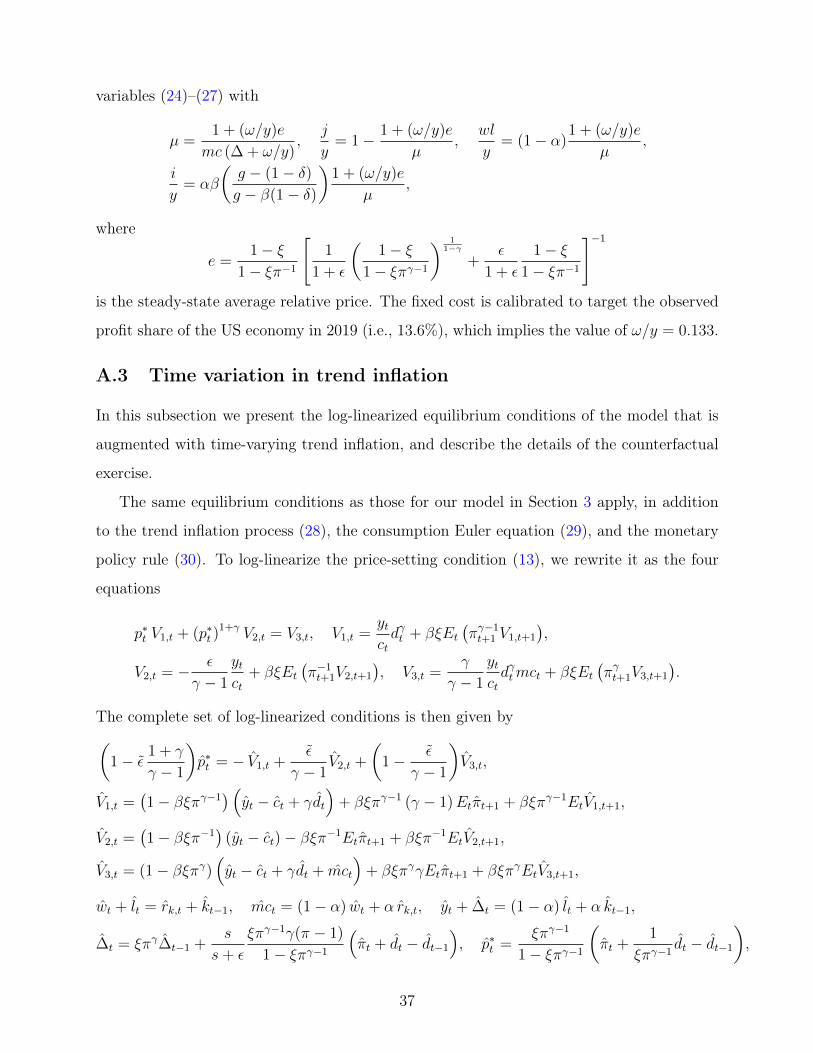
variables (24)–(27) with

µ =1 + (ω/y)e

mc (∆ + ω/y),

j

y= 1− 1 + (ω/y)e

µ,

wl

y= (1− α)

1 + (ω/y)e

µ,

i

y= αβ

(g − (1− δ)g − β(1− δ)

)1 + (ω/y)e

µ,

where

e =1− ξ

1− ξπ−1

[1

1 + ε

(1− ξ

1− ξπγ−1

) 11−γ

+ε

1 + ε

1− ξ1− ξπ−1

]−1is the steady-state average relative price. The fixed cost is calibrated to target the observed

profit share of the US economy in 2019 (i.e., 13.6%), which implies the value of ω/y = 0.133.

A.3 Time variation in trend inflation

In this subsection we present the log-linearized equilibrium conditions of the model that is

augmented with time-varying trend inflation, and describe the details of the counterfactual

exercise.

The same equilibrium conditions as those for our model in Section 3 apply, in addition

to the trend inflation process (28), the consumption Euler equation (29), and the monetary

policy rule (30). To log-linearize the price-setting condition (13), we rewrite it as the four

equations

p∗t V1,t + (p∗t )1+γ V2,t = V3,t, V1,t =

ytctdγt + βξEt

(πγ−1t+1 V1,t+1

),

V2,t = − ε

γ − 1

ytct

+ βξEt(π−1t+1V2,t+1

), V3,t =

γ

γ − 1

ytctdγtmct + βξEt

(πγt+1V3,t+1

).

The complete set of log-linearized conditions is then given by(1− ε 1 + γ

γ − 1

)p∗t = − V1,t +

ε

γ − 1V2,t +

(1− ε

γ − 1

)V3,t,

V1,t =(1− βξπγ−1

) (yt − ct + γdt

)+ βξπγ−1 (γ − 1)Etπt+1 + βξπγ−1EtV1,t+1,

V2,t =(1− βξπ−1

)(yt − ct)− βξπ−1Etπt+1 + βξπ−1EtV2,t+1,

V3,t = (1− βξπγ)(yt − ct + γdt + mct

)+ βξπγγEtπt+1 + βξπγEtV3,t+1,

wt + lt = rk,t + kt−1, mct = (1− α) wt + α rk,t, yt + ∆t = (1− α) lt + α kt−1,

∆t = ξπγ∆t−1 +s

s+ ε

ξπγ−1γ(π − 1)

1− ξπγ−1(πt + dt − dt−1

), p∗t =

ξπγ−1

1− ξπγ−1

(πt +

1

ξπγ−1dt − dt−1

),

37

dt =ξπ−1(1 + ε1π

γ)

1 + ε1dt−1 −

ε1ξπ−1(πγ − 1)

(1 + ε1)(1− ξπ−1)πt, wt =

1

χlt + ct,

kt =1− δg

kt−1 +

(1− 1− δ

g

)it, Etct+1 − ct =

[1− β(1− δ)

g

]Etrk,t+1,

Etct+1 − ct = rt − Etπt+1, yt =c

yct +

i

yit, rt = φπ (πt − π∗t ) , π∗t = ρππ

∗t−1 + εt,

µt = − mct − ∆t, jst =1

µ− 1µt, lst = − µt, ist = it − yt,

where hatted variables denote log-deviations from their steady-state values (e.g., yt = log yt−

log y) and the following definitions are employed: jst ≡ jt/yt, lst ≡ lt/yt, ist ≡ it/yt, and

ε1 ≡ ε[(1− ξ)/(1− ξπγ−1)]γ/(γ−1).

To calibrate the model, the autoregressive process xt = β0 + β1xt−1 + et is estimated by

OLS for the trend inflation series of Chan et al. (2018) during the period from 1960Q2 to

2019Q4. The OLS estimators of β0 and β1 are computed as b0 = 0.000 and b1 = 0.996, and the

Newey-West robust standard errors are s0 = 0.000 and s1 = 0.011, respectively. To conduct

the counterfactual exercise, initial values of the four state variables (π∗t−1,∆t−1, dt−1, kt−1)

must be pinned down. The initial value of the lagged inflation target is set equal to the

trend inflation rate in 1960Q2 in the series of Chan et al. (2018), while those of the other

three (endogenous) state variables are set at their steady-state values.33 Given the initial

values, the trend inflation series is replicated, and the associated counterfactual series for the

average markup, the profit share, the labor share, and the investment share are generated,

by feeding the OLS residuals {xt − b0 − b1xt−1}2019Q4t=1960Q3 into the calibrated model.

B Model with superstar firms

This appendix describes the model with superstar firms, which extends the baseline model

presented in Section 3 by considering two types of firms: ordinary firms f ∈ [0, n], whose

type is indexed by subscript i = 1, and highly productive superstar firms f ∈ (n, 1], whose

type is indexed by subscript i = z. The decision problems of the representative household

and the representative composite-good producer remain unchanged in the extended model.

Firms’ production function (10) is extended to the form (31), so that if z = 1 then the

33Varying the initial values of the three endogenous state variables by ±5% does not alter the qualitativecomparison to the results obtained with the baseline model (as reported in panel (b) of Table 3).

38

extended model is reduced to the baseline model. All firms continue to choose an identical

capital–labor ratio, so that

α

1− αWt

rk,t=K1,t−1

l1,t=Kz,t−1

lz,t,

where K1,t−1 =∫ n0Kt(f) df , l1,t =

∫ n0lt(f) df , Kz,t−1 =

∫ 1

nKt(f) df , and lz,t =

∫ 1

nlt(f) df . In

addition, the real marginal cost is given by the extended form (32); we denotemc1,t = mct(f)

for f ∈ [0, n] and mcz,t = mct(f) for f ∈ (n, 1].

The first-order condition of the price-setting problem for each firm type i ∈ {1, z} can be

written as

Et

∞∑j=0

(βξ)jYt+jCt+j

[(p∗i,tdt+j

)−γ j∏k=1

πγt+k

(p∗i,t

j∏k=1

π−1t+k −γ

γ − 1mci,t+j

)− ε

γ − 1p∗i,t

j∏k=1

π−1t+k

]= 0,

where p∗i,t ≡ P ∗i,t/Pt and P ∗i,t is the price set by firms that can change prices in period t.

Moreover, the law of motion (14) for dt is extended to

d1−γt = d1−γ1,t + d1−γz,t ,

d1−γ1,t = ξ πγ−1t d1−γ1,t−1 + (1− ξ)n(p∗1,t)1−γ

,

d1−γz,t = ξ πγ−1t d1−γz,t−1 + (1− ξ)(1− n)(p∗z,t)1−γ

,

where d1,t ≡[∫ n

0(Pt(f)/Pt)

1−γ df]1/(1−γ)

and dz,t ≡[∫ 1

n(Pt(f)/Pt)

1−γ df]1/(1−γ)

. Similarly,

the law of motion (15) for et is extended to

et = e1,t + ez,t,

e1,t = ξ π−1t e1,t−1 + (1− ξ)n p∗1,t,

ez,t = ξ π−1t ez,t−1 + (1− ξ)(1− n) p∗z,t,

where e1,t ≡∫ n0

(Pt(f)/Pt) df and ez,t ≡∫ 1

n(Pt(f)/Pt) df .

Aggregating the production function (31) for ordinary firms f ∈ [0, n] and for superstar

firms f ∈ (n, 1] leads to, respectively,

Yt ∆1,t = At l1−α1,t K

α1,t−1, (36)

Yt ∆z,t = At l1−αz,t K

αz,t−1, (37)

39

where

∆1,t =s1,t + nε

1 + ε, (38)

∆z,t =sz,t + (1− n)ε

1 + ε(39)

denote the relative price distortions that respectively affect the production of ordinary and

superstar firms, s1,t ≡∫ n0

[Pt(f)/(Pt dt)]−γ df , and sz,t ≡

∫ 1

n[Pt(f)/(Pt dt)]

−γ df . Therefore,

the aggregate production function (18) is replaced with ordinary and superstar firms’ aggre-

gate production functions (36) and (37), and the relative price distortion (16) is replaced

with the two relative price distortions (38) and (39). The laws of motion for s1,t and sz,t are

given by

d−γt s1,t = ξπγt d−γt−1s1,t−1 + (1− ξ)n

(p∗1,t)−γ

,

d−γt sz,t = ξπγt d−γt−1sz,t−1 + (1− ξ)(1− n)

(p∗z,t)−γ

,

which replace the law of motion (19) for st.

The cost-weighted average markup can then be calculated as

µt =

∫ 1

0

TCt(f)∫ 1

0TCt(f) df

Pt(f)

Ptmct(f)df =

1

mc1,t ∆1,t +mcz,t ∆z,t

.

The equilibrium conditions in terms of detrended variables lead to the relevant steady-

state equations

mci =γ − 1

γ

1− βξπγ

1− βξπγ−1

[1− ε

γ − 1

(p∗id

)γ1− βξπγ−1

1− βξπ−1

]p∗i , i ∈ {1, z};

∆1 = n

[1

1 + ε

1− ξ1− ξπγ

(d

p∗1

)γ+

ε

1 + ε

]; ∆z = (1− n)

[1

1 + ε

1− ξ1− ξπγ

(d

p∗z

)γ+

ε

1 + ε

];

d1−γ = d1−γ1 + d1−γz ; d1 =

[(1− ξ)n

1− ξπγ−1

] 11−γ

p∗1; dz =

[(1− ξ)(1− n)

1− ξπγ−1

] 11−γ

p∗z;

e = e1 + ez; e1 =(1− ξ)n1− ξπ−1

p∗1; ez =(1− ξ)(1− n)

1− ξπ−1p∗z; 1 =

1

1 + εd+

ε

1 + εe .

Combining the steady-state equations yields the following three nonlinear equations for the

three steady-state variables {d, p∗1, p∗z}:

1 =1

1 + εd+

ε

1 + ε

1− ξ1− ξπ−1

[np∗1 + (1− n)p∗z] ,

40

d1−γ =(1− ξ)n

1− ξπγ−1(p∗1)

1−γ +(1− ξ)(1− n)

1− ξπγ−1(p∗z)

1−γ ,[γ − 1− ε1− βξπ

γ−1

1− βξπ−1

(p∗1d

)γ ]p∗1 =

[γ − 1− ε1− βξπ

γ−1

1− βξπ−1

(p∗zd

)γ ](z p∗z) , (40)

which can be solved numerically using the values of model parameters presented in Table 2,

z = 1.6, and n = 0.86. The solution allows us to calculate the steady-state real marginal costs

mc1, mcz; the steady-state relative price distortions ∆1, ∆z; the steady-state average markup

(33); the steady-state profit share (25); the steady-state labor share (26); the steady-state

investment share (27); and the density function for the steady-state markup distribution

(34).

In the model with superstar firms the non-CES aggregator plays a dual role: it serves

as not only a source of endogenous variation of firms’ desired markups but also a source

of markup heterogeneity between firms with different productivity levels. The following

proposition shows that, for the two types of firms with product prices of the same age, a

superstar firm has a higher markup in steady state than an ordinary firm if and only if the

aggregator is the non-CES one, i.e., ε < 0.

Proposition 1 Assume that the assumption (21) holds and that z > 1. Consider ordinaryfirms and superstar firms whose product prices have remained unchanged for j periods. Then,the steady-state markup of the superstar firms exceeds that of the ordinary firms if and onlyif ε < 0.

Proof. Let the steady-state markup of a firm of type i ∈ {1, z} with a price of age j bedenoted by µi,j = p∗i / (mci π

j). The proposition then claims that µ1,j < µz,j iff ε < 0.First, assume ε < 0 and suppose the contrary µ1,j ≥ µz,j. Then, mc1 = z mcz implies that

p∗1 ≥ z p∗z > p∗z. Without loss of generality, we have γ−1−ε1−βξπγ−1

1−βξπ−1

(p∗1d

)γ= γ 1−βξπγ−1

1−βξπγmc1p∗16= 0

under the assumption (21). Then, from eq. (40), it follows that

γ − 1− ε1−βξπγ−1

1−βξπ−1

(p∗zd

)γγ − 1− ε1−βξπγ−1

1−βξπ−1

(p∗1d

)γ (z p∗z) = p∗1 ≥ z p∗z ⇔γ − 1− ε1−βξπγ−1

1−βξπ−1

(p∗zd

)γγ − 1− ε1−βξπγ−1

1−βξπ−1

(p∗1d

)γ ≥ 1.

If γ − 1 − ε1−βξπγ−1

1−βξπ−1

(p∗1d

)γ= γ 1−βξπγ−1

1−βξπγmc1p∗1

> 0, we have that γ > 0 and (p∗z)γ ≥ (p∗1)

γ underthe assumption (21). Then, it follows that (p∗z)

γ ≥ (p∗1)γ > (p∗z)

γ, which is a contradiction. Ifγ − 1− ε1−βξπγ−1

1−βξπ−1

(p∗1d

)γ= γ 1−βξπγ−1

1−βξπγmc1p∗1

< 0, we have that γ < 0 and (p∗z)γ ≤ (p∗1)

γ under theassumption (21). Then, it follows that (p∗z)

−γ ≥ (p∗1)−γ > (p∗z)

−γ, which is a contradiction.Next, assume that µ1,j < µz,j and suppose the contrary ε = 0. Then, eq. (40) can

be reduced, without loss of generality, to p∗1 = z p∗z. From mc1 = z mcz, it follows thatµ1,j = µz,j > µ1,j, which is a contradiction.

41

References

Akcigit, Ufuk and Sina T. Ates (2021). “Ten facts on declining business dynamism and

lessons from endogenous growth theory.” American Economic Journal: Macroeconomics,

13(2), pp. 257–298.

Alvarez, Fernando, Martin Beraja, Martín Gonzalez-Rozada, and Pablo Andrés Neumeyer

(2019). “From hyperinflation to stable prices: Argentina’s evidence on menu cost models.”

Quarterly Journal of Economics, 134(1), pp. 451–505.

Ascari, Guido, Louis Phaneuf, and Eric R. Sims (2018). “On the welfare and cyclical impli-

cations of moderate trend inflation.” Journal of Monetary Economics, 99, pp. 56–71.

Ascari, Guido and Argia M. Sbordone (2014). “The macroeconomics of trend inflation.”

Journal of Economic Literature, 52(3), pp. 679–739.

Aum, Sangmin and Yongseok Shin (2020). “Why is the labor share declining?” Federal

Reserve Bank of St Louis Review, 102(4), pp. 413–428.

Autor, David, David Dorn, Lawrence F. Katz, Christina Patterson, and John Van Reenen

(2020). “The fall of the labor share and the rise of superstar firms.” Quarterly Journal of

Economics, 135(2), pp. 645–709.

Banerjee, Anindya and Bill Russell (2001). “The relationship between the markup and

inflation in the G7 economies and Australia.” Review of Economics and Statistics, 83(2),

pp. 377–384.

Banerjee, Anindya and Bill Russell (2005). “Inflation and measures of the markup.” Journal

of Macroeconomics, 27, pp. 289–306.

Barkai, Simcha (2020). “Declining labor and capital shares.” Journal of Finance, 75(5), pp.

2421–2463.

Basu, Susanto (1995). “Intermediate goods and business cycles: Implications for productivity

and welfare.” American Economic Review, 85(3), pp. 512–531.

Basu, Susanto (2019). “Are price-cost markups rising in the United States? A discussion of

the evidence.” Journal of Economic Perspectives, 33(3), pp. 3–22.

Beck, Günther and Sarah M. Lein (2020). “Price elasticities and demand-side real rigidities

in micro data and in macro models.” Journal of Monetary Economics, 115, pp. 200–212.

42

Bénabou, Roland (1988). “Search, price setting and inflation.” Review of Economic Studies,

55(3), pp. 353–376.

Bénabou, Roland (1992). “Inflation and markups: Theories and evidence from the retail

trade sector.” European Economic Review, 36(2–3), pp. 566–574.

Borio, Claudio and Andrew Filardo (2007). “Globalization and inflation: New cross-country

evidence on the global determinants of domestic inflation.” BIS Working Papers 227, Bank

for International Settlements.

Calvo, Guillermo A. (1983). “Staggered prices in a utility-maximizing framework.” Journal

of Monetary Economics, 12(3), pp. 383–398.

Candia, Bernardo, Olivier Coibion, and Yuriy Gorodnichenko (2021). “The inflation expecta-

tions of U.S. firms: Evidence from a new survey.” Working Paper 28836, National Bureau

of Economic Research.

Carlton, Dennis W. (1986). “The rigidity of prices.” American Economic Review, 76(4), pp.

637–658.

Chan, Joshua C.C., Todd E. Clark, and Gary Koop (2018). “A new model of inflation, trend

inflation, and long-run inflation expectations.” Journal of Money, Credit and Banking,

50(1), pp. 5–53.

Chen, Natalie, Jean Imbs, and Andrew Scott (2004). “Competition, globalization, and the

decline of inflation.” CEPR Discussion Papers 4695, Centre for Economic Policy Research.

Cogley, Timothy and Argia M. Sbordone (2008). “Trend inflation, indexation, and inflation

persistence in the New Keynesian Phillips curve.” American Economic Review, 98(5), pp.

2101–2126.

Covarrubias, Matias, Germán Gutiérrez, and Thomas Philippon (2020). “From good to bad

concentration? U.S. industries over the past 30 years.” In Martin S. Eichenbaum, Erik

Hurst, and Jonathan A. Parker, editors, NBER Macroeconomics Annual 2019, volume 34,

chapter 1, pp. 1–46. University of Chicago Press.

De Loecker, Jan, Jan Eeckhout, and Gabriel Unger (2020). “The rise of market power and

the macroeconomic implications.” Quarterly Journal of Economics, 135(2), pp. 561–644.

Dixon, Huw and Engin Kara (2006). “How to compare Taylor and Calvo contracts: A

comment on Michael Kiley.” Journal of Money, Credit and Banking, 38(4).

Dossche, Maarten, Freddy Heylen, and Dirk Van den Poel (2010). “The kinked demand curve

43

and price rigidity: Evidence from scanner data.” Scandinavian Journal of Economics,

112(4), pp. 723–752.

Dotsey, Michael and Robert G. King (2005). “Implications of state-dependent pricing for

dynamic macroeconomic models.” Journal of Monetary Economics, 52(1), pp. 213–242.

Edmond, Chris, Virgiliu Midrigan, and Daniel Yi Xu (2018). “How costly are markups?”

NBER Working Paper 24800, National Bureau of Economic Research.

Edmond, Chris, Virgiliu Midrigan, and Daniel Yi Xu (2021). “How costly are markups?”

Working paper.

Eichenbaum, Martin and Jonas D. M. Fisher (2007). “Estimating the frequency of price

re-optimization in Calvo-style models.” Journal of Monetary Economics, 54(7), pp. 2032–

2047.

Elsby, Michael W. L., Bart Hobijn, and Aysegul Sahin (2013). “The decline of the U.S. labor

share.” Brookings Papers on Economic Activity, (Fall), pp. 1–52.

Erceg, Christopher J., Dale W. Henderson, and Andrew T. Levin (2000). “Optimal monetary

policy with staggered wage and price contracts.” Journal of Monetary Economics, 46(2),

pp. 281–313.

Friedman, Milton (1968). “The role of monetary policy.” American Economic Review, 58(1),

pp. 1–17.

Galí, Jordi and Mark Gertler (1999). “Inflation dynamics: A structural econometric analysis.”

Journal of Monetary Economics, 44(2), pp. 195–222.

Gopinath, Gita and Oleg Itskhoki (2011). “In search of real rigidities.” In Daron Acemoglu

and Michael Woodford, editors, NBER Macroeconomics Annual 2010, volume 25, chap-

ter 5, pp. 261–309. University of Chicago Press.

Gorodnichenko, Yuriy and Michael Weber (2016). “Are sticky prices costly? Evidence from

the stock market.” American Economic Review, 106(1), pp. 165–199.

Guerrieri, Luca, Christopher Gust, and J. David López-Salido (2010). “International compe-

tition and inflation: A New Keynesian perspective.” American Economic Journal: Macroe-

conomics, 2(4), pp. 247–280.

Gutiérrez, Germán and Thomas Philippon (2017). “Investment-less growth: An empirical

investigation.” Brookings Papers on Economic Activity, (Fall), pp. 89–169.

44

Hall, Robert E. (2018). “Using empirical marginal cost to measure market power in the US

economy.” Working Paper 25251, National Bureau of Economic Research.

Hirose, Yasuo, Takushi Kurozumi, and Willem Van Zandweghe (2020). “Monetary policy

and macroeconomic stability revisited.” Review of Economic Dynamics, 37, pp. 255–274.

Hirose, Yasuo, Takushi Kurozumi, and Willem Van Zandweghe (2021). “Inflation gap persis-

tence, indeterminacy, and monetary policy.” Working Paper 21-05, Federal Reserve Bank

of Cleveland.

Ireland, Peter N. (2007). “Changes in the Federal Reserve’s inflation target: Causes and

consequences.” Journal of Money, Credit and Banking, 39(8), pp. 1851–1882.

Jordà, Òscar, Sanjay R. Singh, and Alan M. Taylor (2020). “The long-run effects of monetary

policy.” Working Paper 26666, National Bureau of Economic Research.

Karabarbounis, Loukas and Brent Neiman (2014). “The global decline of the labor share.”

Quarterly Journal of Economics, 129(1), pp. 61–103.

Karabarbounis, Loukas and Brent Neiman (2019). “Accounting for factorless income.” In

Martin Eichenbaum and Jonathan A. Parker, editors, NBER Macroeconomics Annual

2018, volume 33, chapter 3, pp. 167–228. University of Chicago Press.

Kehrig, Matthias and Nicolas Vincent (2021). “The micro-level anatomy of the labor share

decline.” Quarterly Journal of Economics, 136(2), pp. 1031–1087.

Kimball, Miles S. (1995). “The quantitative analytics of the basic neomonetarist model.”

Journal of Money, Credit and Banking, 27(4), pp. 1241–1277.

King, Robert G. and Alexander L. Wolman (1996). “Inflation targeting in a St. Louis model

of the 21st century.” Federal Reserve Bank of St Louis Review, 78 (May/June), pp. 83–107.

Klenow, Peter J. and Benjamin A. Malin (2010). “Microeconomic evidence on price-setting.”

In Benjamin M. Friedman and Michael Woodford, editors, Handbook of Monetary Eco-

nomics, volume 3A, chapter 6, pp. 231–284. Elsevier.

Klenow, Peter J. and Jonathan L. Willis (2016). “Real rigidities and nominal price changes.”

Economica, 83, pp. 443–472.

Kreps, David M. (1998). “Anticipated utility and dynamic choice.” In Donald P. Jacobs,

Ehud Kalai, and Morton I. Kamien, editors, Frontiers of Research in Economic Theory:

The Nancy L. Schwartz Memorial Lectures, 1983–1997, volume 3A, chapter 9, pp. 242–

274. Cambridge University Press.

45

Kurozumi, Takushi and Willem Van Zandweghe (2016). “Kinked demand curves, the natural

rate hypothesis, and macroeconomic stability.” Review of Economic Dynamics, 20, pp.

240–257.

Kurozumi, Takushi and Willem Van Zandweghe (2020). “Output-inflation trade-offs and the

optimal inflation rate.” Working Paper 20-20, Federal Reserve Bank of Cleveland.

Levin, Andrew T., J. David López-Salido, Edward Nelson, and Tack Yun (2008). “Macroeco-

nomic equivalence, microeconomic dissonance, and the design of monetary policy.” Journal

of Monetary Economics, 55(Supplement), pp. S48–S62.

L’Huillier, Jean-Paul and Raphael Schoenle (2021). “Raising the inflation target: What are

the effective gains in policy room?” Working paper, Brandeis University.

Meier, Matthias and Timo Reinelt (2021). “Monetary policy, markup dispersion, and aggre-

gate TFP.” Working paper, University of Mannheim.

Moran, Patrick and Albert Queralto (2018). “Innovation, productivity, and monetary policy.”

Journal of Monetary Economics, 93, pp. 24–41.

Nakamura, Emi and Jón Steinsson (2010). “Monetary non-neutrality in a multisector menu

cost model.” Quarterly Journal of Economics, 125(3), pp. 961–1013.

Nakamura, Emi, Jón Steinsson, Patrick Sun, and Daniel Villar (2018). “The elusive costs

of inflation: Price dispersion during the U.S. Great Inflation.” Quarterly Journal of Eco-

nomics, 133(4), pp. 1933–1980.

Pasten, Ernesto, Raphael Schoenle, and Michael Weber (2020). “The propagation of mon-

etary policy shocks in a heterogeneous production economy.” Journal of Monetary Eco-

nomics, 116, pp. 1–22.

Rogoff, Kenneth S. (2004). “Globalization and global disinflation.” In Monetary Policy

and Uncertainty: Adapting to a Changing Economy, pp. 77–112. Federal Reserve Bank of

Kansas City.

Rotemberg, Julio J. (1982). “Sticky prices in the United States.” Journal of Political Econ-

omy, 90(6), pp. 1187–1211.

Schmitt-Grohé, Stephanie and Martín Uribe (2010). “The optimal rate of inflation.” In

Benjamin M. Friedman and Michael Woodford, editors, Handbook of Monetary Economics,

volume 3B, chapter 13, pp. 653–722. Elsevier.

46

Smets, Frank and Rafael Wouters (2007). “Shocks and frictions in US business cycles: A

Bayesian DSGE approach.” American Economic Review, 97(3), pp. 586–606.

Syverson, Chad (2019). “Macroeconomics and market power: context, implications, and

open questions.” Journal of Economic Perspectives, 33(3), pp. 23–43.

Taylor, John B. (1980). “Aggregate dynamics and staggered contracts.” Journal of Political

Economy, 88(1), pp. 1–23.

Taylor, John B. (1993). “Discretion versus policy rules in practice.” Carnegie-Rochester

Conference Series on Public Policy, 39, pp. 195–214.

Zbaracki, Mark J., Mark Ritson, Daniel Levy, Shantanu Dutta, and Mark Bergen (2004).

“Managerial and customer costs of price adjustment: Direct evidence from industrial mar-

kets.” Review of Economics and Statistics, 86(2), pp. 514–533.

47