capital structure, macroeconomic environment, firm's - UoN ...
181
CAPITAL STRUCTURE, MACROECONOMIC ENVIRONMENT, FIRM’S EFFICIENCY AND VALUE OF COMPANIES LISTED AT THE NAIROBI SECURITIES EXCHANGE JOHN NJERU NJAGI A RESEARCH THESIS SUBMITTED IN PARTIAL FULFILMENT FOR THE REQUIREMENTS OF THE AWARD OF THE DEGREE OF DOCTOR OF PHILOSOPHY IN BUSINESS ADMINISTRATION UNIVERSITY OF NAIROBI 2017
-
Upload
khangminh22 -
Category
Documents
-
view
1 -
download
0
Transcript of capital structure, macroeconomic environment, firm's - UoN ...
CAPITAL STRUCTURE, MACROECONOMIC ENVIRONMENT, FIRM’S
EFFICIENCY AND VALUE OF COMPANIES LISTED AT THE NAIROBI
SECURITIES EXCHANGE
JOHN NJERU NJAGI
A RESEARCH THESIS SUBMITTED IN PARTIAL FULFILMENT FOR THE
REQUIREMENTS OF THE AWARD OF THE DEGREE OF DOCTOR OF
PHILOSOPHY IN BUSINESS ADMINISTRATION UNIVERSITY OF NAIROBI
2017

ii
DECLARATION

iii
COPYRIGHT
All rights reserved. No part of this thesis may be reproduced either in part or whole without
prior written permission from the author or the University of Nairobi, except in the case of
brief quotations embodied in review articles and research papers. Making copies of any
part of this thesis for any purpose other than personal use is a violation of the Kenyan and
international Copyright laws. For information, contact John Njagi at the following address:
P.O. Box 1542-00100
Nairobi
Telephone: 0729-057-918
E-mail: [email protected]

iv
DEDICATION
I dedicate this Doctoral thesis first to my dear parents. Ann Njagi and the late Dionisio
Njagi for giving me the foundation and motivation to seek great heights academically.
Secondly my supportive and understanding immediate family Daisy Njagi and Joysheilla
Gatwiri.

v
ACKNOWLEDGEMENT
My utmost gratitude to the good Lord for he has kept me safe this far. It’s through mighty
hand of God that this work was made possible.
I would also like to express my sincere appreciation to every individual who has
contributed towards the success of this study including my supervisors, mentors colleagues
and various organizations who played a role in the completion of this research thesis.
I am highly indebted to Prof Josiah Aduda, Dr Erastus Sifunjo and Dr Cyrus Iraya for the
invaluable support and guidance they accorded me during this rigorous academic journey.
I am grateful and sincerely thank you for your patience, encouragement and helpful
comments you provided during the entire study period, without yourself and insightful
comments I would not have stretched this far.
I wish to record my appreciation to the team at CMA led by Mr. Geoffrey Ruto and KNBS
team lead by Mr. Robert Mwaniki for availing the relevant data. I extend my utmost
gratitude to the listed companies that formed part of this study. I am deeply indebted to all
the parties whom contributed to the successful completion of this thesis. May the Almighty
Lord bless you abundantly.

vi
TABLE OF CONTENTS
DECLARATION............................................................................................................... ii
COPYRIGHT .................................................................................................................... ii
DEDICATION.................................................................................................................. iv
ACKNOWLEDGEMENT ................................................................................................ v
LIST OF TABLES ........................................................................................................... xi
LIST OF FIGURES ....................................................................................................... xiii
ABBREVIATIONS AND ACRONYMS ...................................................................... xiv
ABSTRACT ..................................................................................................................... xv
CHAPTER ONE: INTRODUCTION ............................................................................. 1
1.1 Background of the Study ........................................................................................... 1
1.1.1 Capital Structure .............................................................................................. 3
1.1.2 Macroeconomic Environment ......................................................................... 4
1.1.3 Firm efficiency ................................................................................................ 6
1.1.4 Firm Value ..................................................................................................... 12
1.1.5 Nairobi Securities Exchange ......................................................................... 13
1.2 Statement of the Problem ........................................................................................ 14
1.3 Objectives of the Study ........................................................................................... 18
1.3.1 General Objective ................................................................................................. 18
1.3.2 Specific Objectives ........................................................................................ 18
1.4 Value of the Study ................................................................................................... 19
1.5 Organization of the Study ....................................................................................... 21
CHAPTER TWO: LITERATURE REVIEW .............................................................. 23
2.1 Introduction ............................................................................................................. 23
2.2 Theoretical Review ................................................................................................. 23
2.2.1 Modigliani and Miller Theory of Capital Structure ...................................... 23
2.2.2 The Pecking Order Theory ............................................................................ 27
2.2.3 The Trade-Off Model .................................................................................... 29
2.2.4 Agency Theory .............................................................................................. 30

vii
2.2.5 Transaction Cost Theory ............................................................................... 32
2.2.6 Resource Based Theory ................................................................................. 33
2.3 Firm Value Measurement ........................................................................................ 35
2.3.1 Parametric Approaches to Performance Measurement of Firms ................... 36
2.3.2 Non Parametric Approaches to Performance Measurement of Firms ........... 37
2.3.3 Parametric Versus Non-Parametric Approaches ........................................... 38
2.4 Review of Empirical Literature ............................................................................... 41
2.4.1 Capital Structure and Firm Value .................................................................. 41
2.4.2 Capital Structure, Macroeconomic Environment and Firm Value ................ 43
2.4.3 Capital Structure, Firm efficiency and Firm Value ....................................... 44
2.4.4 Capital Structure, Economic Environment, Firm efficiency and Value ........ 50
2.5 Summary of Literature and the Knowledge Gaps ................................................... 50
2.6 Conceptual Framework ........................................................................................... 58
CHAPTER THREE: RESEARCH METHODOLOGY ............................................. 60
3.1 Introduction ............................................................................................................. 60
3.2 Research Philosophy ............................................................................................... 60
3.3 Research Design ...................................................................................................... 61
3.4 Population of the Study ........................................................................................... 62
3.5 Sample of the Study ................................................................................................ 62
3.6 Data and Data Collection Instruments .................................................................... 62
3.7 Diagnostic Testing................................................................................................... 63
3.7.1 Tests for Multicollinearity ............................................................................. 64
3.7.2 Panel Level Stationarity ................................................................................ 64
3.7.3 Serial Correlation .......................................................................................... 64
3.7.4 Likelihood Ratio Test for Heteroscedasticity ................................................ 65
3.7.5 Model Fitting ................................................................................................. 65
3.8 Operationalization of the Research Variables and Measurements .......................... 66
3.9 Data Analysis .......................................................................................................... 68
3.9.1 Data Analysis Techniques ............................................................................. 68
viii
3.9.2 Empirical Model for Testing Hypothesis One: Effect of Capital Structure
on Firm Value ................................................................................................ 68
3.9.3 Empirical Models for Testing Hypothesis Two: Moderating Effect of
Macroeconomic Environment ....................................................................... 69
3.9.4 Empirical Models for testing Hypothesis Three: Intervening Effect of
Firm’s efficiency ........................................................................................... 72
3.9.5 Empirical Model for Testing Hypothesis Four: Joint Effect of Capital
Structure, Macroeconomic Environment, and Firm’s efficiency on Firm
Value. ............................................................................................................ 73
CHAPTER FOUR: DESCRIPTIVE DATA ANALYSIS AND PRESENTATION . 77
4.1 Introduction ............................................................................................................. 77
4.2 Study Sample........................................................................................................... 77
4.3 Research Design ...................................................................................................... 77
4.4 Descriptive Statistics ............................................................................................... 78
4.5 Correlation Analysis ................................................................................................ 80
4.6 Chapter Summary .................................................................................................... 86
CHAPTER FIVE: HYPOTHESES TESTING AND DISCUSSION OF
FINDINGS ....................................................................................................................... 90
5.1 Introduction ............................................................................................................. 90
5.1.1 Diagnostic Testing ......................................................................................... 90
5.1.2 Model Fitting ................................................................................................. 92
5.2 Relationship between Capital Structure and the Value of the Firm ........................ 93
5.2.1 Model Fitting ................................................................................................. 95
5.3 Moderating Effect of Macroeconomic Environment on the Relationship between
Capital Structure and the Value of the Firm ........................................................... 97
5.3.1 Step One of Testing the Moderating Effect: Estimate Joint Effect of
Independent Variable and Moderating Variable on Dependent Variable ..... 98

ix
5.3.2 Step Two of Testing the Moderating Effect: Estimate Joint Effect of
Independent Variable, Moderating Variable and Interaction Terms on
Dependent Variable ..................................................................................... 102
5.4 Intervening Effect of Firm efficiency on the Relationship between Capital
Structure and the Value of the Firm ..................................................................... 108
5.4.1 Step One of Testing the Intervening Effect: Estimate Effect of Independent
Variable on Dependent Variable ................................................................. 109
5.4.2 Step Two of Testing the Intervening Effect: Estimate Effect of Independent
Variable on Intervening Variable ................................................................ 110
5.5 Joint Effect of Capital Structure, Macroeconomic Environment and Firm
Efficiency on the Value of the Firm ..................................................................... 119
5.6 Discussion of the Research Findings .................................................................... 123
5.6.1 Relationship between Capital Structure and Firm Value ............................ 123
5.6.2 Moderating Influence of Macroeconomic Environment in the Relationship
between Capital Structure and Firm Value ................................................. 124
5.6.3 Intervening Effects of Firm’s efficiency in the Relationship between
Capital Structure and Firm Value ................................................................ 126
5.6.4 Joint Effects of Capital Structure, Macroeconomic Environment, Firm’s
efficiency and Firm Value ........................................................................... 127
5.7 Chapter Summary .................................................................................................. 128
CHAPTER SIX: SUMMARY, CONCLUSIONS AND RECOMMENDATIONS . 130
6.1 Introduction ........................................................................................................... 130
6.2 Summary of the Study ........................................................................................... 130
6.3 Conclusions of the Study....................................................................................... 134
6.4 Contributions of the Study Findings ..................................................................... 136
6.4.1 Contributions to Knowledge ....................................................................... 136
6.4.2 Contributions to Managerial Policy and Practices ...................................... 138
6.5 Limitations of the Study ........................................................................................ 140
6.6 Recommendations for Further Research ............................................................... 141
x
REFERENCES .............................................................................................................. 142
APPENDICES ............................................................................................................... 159
Appendix I: Introduction Letter .................................................................................. 159
Appendix II: Data Collection Form ............................................................................ 160
Appendix III: Listed Companies at NSE..................................................................... 163
Apendix IV: Authorization Letter from NACOSTI .................................................... 165
Appendix V: Research Clearance Permit from NACOSTI ......................................... 166
xi
LIST OF TABLES
Table 2.1: Summary of Literature and Knowledge Gaps ................................................. 54
Figure 2.1: Conceptual Model .......................................................................................... 59
Table 3.1: Operationalization of Study Variables ............................................................. 67
Table 3.2: Interaction Terms of the Independent and Moderating Variables ................... 70
Table 3.3: Summary of Statistical Tests of Hypothesis .................................................... 75
Table 4.1: Summary Statistics for Non-Financial Firms Data for the Period 2009 to
2014 ............................................................................................................... 78
Table 4.2: Correlation between Firm Value and Capital Structure .................................. 81
Table 4.3: Correlation between Firm Value and Macroeconomic Environment .............. 82
Table 4.4: Correlation between Firm Value and Firm’s efficiency .................................. 83
Table 4.5: Correlation between Capital Structure and Macroeconomic Environment ..... 83
Table 4.6: Correlation between Capital Structure and Firm’s efficiency ......................... 85
Table 4.7: Correlation between Macroeconomic Environment and Firm’s efficiency .... 86
Table 5.1: Test for Multicollinearity ................................................................................. 93
Table 5.2: Test for Multicollinearity after Dropping the “Debt Ratio” Independent
Variable ......................................................................................................... 94
Table 5.3: Levin Lin Chu Tests for Panel Level Stationarity ........................................... 94
Table 5.4: Wooldridge Test for Autocorrelation in Panel Data ........................................ 95
Table 5.5: Likelihood-Ratio Test for Heteroscedasticity .................................................. 95
Table 5.6: Prais Winsten Panel Regression with Corrected Standard Errors ................... 96
Table 5.7: Test for Multicollinearity ................................................................................. 98
Table 5.8: Test for Multicollinearity after Dropping the “Debt Ratio” Independent
Variable ......................................................................................................... 99
Table 5.9: Levin Lin Chu Tests for Panel Level Stationarity ........................................... 99
Table 5.10: Wooldridge Test for Autocorrelation in Panel Data .................................... 100
Table 5.11: Likelihood-Ratio Test for Heteroscedasticity .............................................. 100
Table 5.12: Prais Winsten Panel Regression with Corrected Standard Errors ............... 101
Table 5.13: Interaction Terms ......................................................................................... 103
Table 5.14: Test for Multicollinearity ............................................................................. 104
Table 5.15: Levin Lin Chu Tests for Panel Level Stationarity ....................................... 105
Table 5.16: Wooldridge Test for Autocorrelation in Panel Data .................................... 105
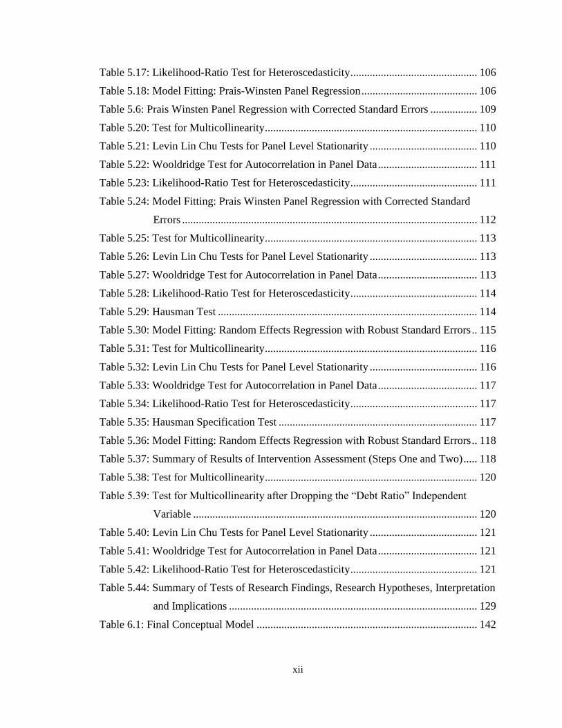
xii
Table 5.17: Likelihood-Ratio Test for Heteroscedasticity .............................................. 106
Table 5.18: Model Fitting: Prais-Winsten Panel Regression .......................................... 106
Table 5.6: Prais Winsten Panel Regression with Corrected Standard Errors ................. 109
Table 5.20: Test for Multicollinearity ............................................................................. 110
Table 5.21: Levin Lin Chu Tests for Panel Level Stationarity ....................................... 110
Table 5.22: Wooldridge Test for Autocorrelation in Panel Data .................................... 111
Table 5.23: Likelihood-Ratio Test for Heteroscedasticity .............................................. 111
Table 5.24: Model Fitting: Prais Winsten Panel Regression with Corrected Standard
Errors ........................................................................................................... 112
Table 5.25: Test for Multicollinearity ............................................................................. 113
Table 5.26: Levin Lin Chu Tests for Panel Level Stationarity ....................................... 113
Table 5.27: Wooldridge Test for Autocorrelation in Panel Data .................................... 113
Table 5.28: Likelihood-Ratio Test for Heteroscedasticity .............................................. 114
Table 5.29: Hausman Test .............................................................................................. 114
Table 5.30: Model Fitting: Random Effects Regression with Robust Standard Errors .. 115
Table 5.31: Test for Multicollinearity ............................................................................. 116
Table 5.32: Levin Lin Chu Tests for Panel Level Stationarity ....................................... 116
Table 5.33: Wooldridge Test for Autocorrelation in Panel Data .................................... 117
Table 5.34: Likelihood-Ratio Test for Heteroscedasticity .............................................. 117
Table 5.35: Hausman Specification Test ........................................................................ 117
Table 5.36: Model Fitting: Random Effects Regression with Robust Standard Errors .. 118
Table 5.37: Summary of Results of Intervention Assessment (Steps One and Two) ..... 118
Table 5.38: Test for Multicollinearity ............................................................................. 120
Table 5.39: Test for Multicollinearity after Dropping the “Debt Ratio” Independent
Variable ....................................................................................................... 120
Table 5.40: Levin Lin Chu Tests for Panel Level Stationarity ....................................... 121
Table 5.41: Wooldridge Test for Autocorrelation in Panel Data .................................... 121
Table 5.42: Likelihood-Ratio Test for Heteroscedasticity .............................................. 121
Table 5.44: Summary of Tests of Research Findings, Research Hypotheses, Interpretation
and Implications .......................................................................................... 129
Table 6.1: Final Conceptual Model ................................................................................ 142

xiii
LIST OF FIGURES
Figure 2.1: Conceptual Model ......................................................................................... 59

xiv
ABBREVIATIONS AND ACRONYMS
CAPM Capital Asset pricing Authorities
CBK Central Bank of Kenya
CMA Capital Market Authority
DISTC Distribution Costs
DEBTR Debt Ratio
EPS Earnings Per Share
EQUITR Equity Ratio
ERM Efficient Resource Management
FINC Financing Costs
GDP Gross Domestic Product
INTR Interest Costs
ITR Inventory Turnover Ratio
JSE Japanese Stock Exchange
M&M Modigliani and Miller
MPS Market Share Price
NPV Net Present Value
NSE Nairobi Securities Exchange
P/E Price Earnings Ratio
RBT Resource Based Theory
RETR Retained Earnings Ratio
ROA Return on Assets
ROE Return on Equity
SCA Sustainable Competitive Advantage
SFA Stochastic Frontier Approach
MSP Market Share Price
TAX Taxation
TCE Transactions Costs Economic
TCT Transaction Cost Theory
TSE Taiwan Securities Exchange
WACC Weighted Average Cost of Capital

xv
ABSTRACT
In financing an organization, its value is dependent on various components such as the
amount of debt, the amount of equity and the amount of retained earnings. The link between
these components can be influenced by predictor and controlling variables. This study
intended to establish how macroeconomic environment and firm efficiency influence the
relation between firm capital structure and value of companies trading on the NSE. The
specific objectives were to establish the influence of capital structure on the value of the
firms trading on NSE and to determine the moderating influence of macroeconomic
environment and the intervening effect of firm efficiency on the link between capital
structure and firm value. The study was anchored on the MM theory of capital structure
and positivistic philosophy.The longitudinal research design was employed and the
population of the study was firms listed at the NSE. For data collection purposes, the
research targeted non-financial firms which actively traded from 2009 to 2014. The study
hypothesized that capital structure impacts on firms value through the moderating influence
of macroeconomic environment and intervening effects of firm efficiency. Data was
analyzed using inferential and descriptive statistics. First, descriptive statistics of the
variables were outlined. Next, secondary panel data from 30 non-financial firms for the
period of six years from 2009 to 2014 was analyzed using STATA 12 statistical software.
In situations where the panel data do not meet all the assumption of regression analysis of
no autocorrelation, data was analyzed by fitting a Prais Winsten Panel Regression model
which gives robust results in the presence of autocorrelation. Morever, panel regression
analysis was conducted using robust corrected standard errors in instances where
heteroscedasticity was present. These interventions were undertaken after diagnostic
testing to ensure credibility of the results even when the classic linear regression (CLRM)
assumptions were not completely met. The findings suggest that capital structure affects
firm value through joint influence of macroeconomic environment and firm efficiency. The
conclusions of this research expand understanding and knowledge within the field of
capital structure, macroeconomic environment and firm value. First, the use of debt to
finance firm operations should be increased to maximize the tax shield available to the
firms, further debt should be used as a displinary role to force firm’s managers to manage
their firms efficiently and equity holders should also exert some control and influence in
management decisions through their representation in the board of directors. Secondly, the
government should provide stability of the macroeconomic environment through its fiscal
and monetary policies to ensure low inflation rate, tax rate, and high economic growth
rate.Thidly firm’s managers should make practical application of agency cost theory
through use of debt in their capital structure as displinary role of debt forcing firm’s
managers to manage firm’s resources efficiently and the government through Capital
Markets Authority (CMA) should develop appropriate policies in an attempt to organize
the debt capital markets to enable Kenyan firms get access to low cost long term debt to
finance their investment.Consequently, the cost of firm operations declines while firm’s
profits increase causing the values of the firm to increase .This study is important since it
has provided direction on how to integrate optimal financing strategy, efficient
management of firm’s resources, utilizing opportunities provided by favourable
macroeconomic environment inorder to realise increased value for Kenyan firms
1
CHAPTER ONE
INTRODUCTION
1.1 Background of the Study
Immense discussions have been done on the association between capital structure and value
of organizations for a long time by both academics and practitioners (Draniceanu, 2013).
Evidence from research has established that capital structure decisions influence firm value
(McConnell and Servaes, 1995; Rathinasamy, Krishnaswamy and Mantripragada, 2002;
and Chowdhury and Chowdhury, 2010) but cannot exhaustively explain variability in firm
value. However, these studies have not exhaustively explained the variability in the value
of the firm (Kadongo, Makoteli & Maina, 2014). This means other variables such
macroeconomic environment and firm’s efficiencies do have implications on the link
between a firm constitution of capital and value.The re-examination of this relationship is
important because the influence of capital structure on the macroeconomic environment
and firm efficiency can increase the firm market value (Tan & Litsschert, 1994).
The prevailing macroeconomic environment determines level of firm profitability and
market value (Porter &Linde, 1995). In the process of formulating policy options that
influence firm value, the organization must take account of macroeconomic forces. When
the macroeconomic environment becomes hostile, as it sometimes does, the resources get
even scarcer, a situation that forces firms to operate in a state of uncertainty which often
results in poor performance (Murgor, 2014). Prevailing macroeconomic environment of a
firm determine its opportunities and threats of the present and future which influence the
beviour of the firm impacting on its market value (Porter, 1985). Similarly firm’s
efficiency in terms of efficient use of resources within a firm can create a competitive
2
advantage and determine firm ability to use its potentials to neutralise its threats and tap its
opportunities (Murgor, 2014). The influence of macroeconomic environment and firm’s
efficiency on the relationship between capital structure and firm value emanates from their
ability to give firms capabilities which are not easily matched by the competitors
(Wernerfelt, 1984).
The above conceptualization is anchored on the modigilian and Miller theory (1958 &
1963) Transaction Cost Theory (TCT) by Williamson (1985), Resource Based Theory
(RBT) by Penrose (1959), Pecking Order Theory by Myers and Majluf (1984), Trade-off
model by Myers (1984) and Agency Theory by Jensen and Meckling, (1976). MM theory
of capital structure dwells on the perfections and imperfections of the market. Under
perfect market conditions the value of the firm is affected by firm operating profitability
rather than its capital structure while presence of corporate tax laws makes the market value
of the firm an increasing function of leverage (Modigliani & Miller, 1963). Transaction
Cost Theory (TCT) aspires to explain how firms internalize its operations and other
structural arrangements required to improve its market value. Similarly the influence of
capital structure on firm efficiency and firm value is underpinned by Resource Based
Theory (RBT). The RBT explains how possession of unique resources and efficient
application of those resources contributes to competitive advantage within a firm and
undoubtedly productivity differences (Ongeti, 2014; Pasanen, 2013).
The Nairobi Securities Exchange (NSE) was formed in 1954 with deliberate intentions by
brokers of shares traded in listed organizations within the confines of Societies Act. In July
2011 upon promulgation of the new constitution in Kenya 2010, Nairobi Stock Exchange
Limited rebranded to Nairobi Securities Exchanges (NSE) to reflect the evolution of NSE
3
into a full service organization that aids in commercial exchange, clearance and transfer of
equities, among other financial assets and trading instruments.
Performance in terms of market value of firms listed at the NSE has been dismal to the
extent that some have lately called for financial bailout while others are being delisted from
the NSE (NSE Hand Book, 2014). However, some firms have performed exceedingly well
despite financing their investment using risky short term financing instruments in place of
less risky financing instruments . This deviates from the existing theoretical thinking which
would have expected different results. Therefore this means that, other factors apart from
financing methods/ instruments emerge to influence and affect the firm performance and
their market value (Kadondo, Makoteli & Maina, 2014).
1.1.1 Capital Structure
Capital structure entails methods through which an organization funds its investments and
operations using retained earnings, debts and equity (Linh, 2014; Desi & Robertson, 2003).
Brealey and Myers (2008) affirm that capital structure is a mix of diverse financial assets
to fund organizational investments. This encompasses funding sources that are considered
long term in nature (Inanga & Ajayi, 1999). Capital structure constitutes the different
proportions of equity and long-term debt (Pandey, 1999)
Maintenance of appropriate capital structure is important for the maximization of returns
on investment and effectiveness in managing competitiveness (Linh, 2014). The prevailing
argument is that suitable structure of funding sources is achieved when there is an
equilibrium between tax savings arising from use of debt and possibility of insolvency.
This equilibrium would provide superior financial benefits to the owners than purely using
4
equity. The eventual effect of the balanced capital structure would be low average cost of
capital coupled with high returns to shareholder; in terms of maximized share price (De
Angelo & Masulis, 1980).
1.1.2 Macroeconomic Environment
According to Galbraith (2006) macroeconomic environment refers to peripheral aspects in
organizations, marketplace and the entire economic spectrum that have an impact on
organizational operations. Macro- economic factors influences the entire economy as well
as business firms either directly or indirectly. Korajczyk and Levy (2003) argues that the
variations in the macroeconomic environment where the firm operates should influence the
future value of a firm. Moreover, they state that macroeconomic conditions are determined
by several factors, key of which are the interest rates, foreign exchange rates, inflation rates
and GDP growth rates that are prevailing in a country.
The real Gross Domestic Product (GDP) portrays economic performance in a country. As
such, the GDP component has been adopted in studies as a moderating factor for economic
performance. The plausible explanation for this assertion is that during periods of economic
boom, business demand more external financing to widen their investment portfolios.
Economic growth underpins firms' alteration of their capital structures. The growth in the
real GDP affects the cost of finances and hence the future value of firms. It is hypothesized
that there is a proportional association between GDP and the real cost of capital (Drobetz
&Wanzenried, 2006).

5
Pressures of inflation heavily impact on the cost of capital. DeAngelo and Masulis (1980)
stated that inflation has a negative impact on cost of debt which could increase debt to
equity ratios. On the contrary, Schall (1984) notes that in case of high inflation, the earnings
on equity are greater than those on debt financing sources. In this case, companies would
consider sale of equity better than issuing debt. Given these variations, it can be
hypothesized that inflation has an influence on which capital structure business embrace
that would eventually affect wealth of the firm and the cost of capital.
The prevailing macroeconomic environment determines the level of firm profitability due
to cost of capital benefits arising from favourable interest rates prevailing in the country
and the growth in GDP which provides more business opportunities for the firm. Moreover,
favourable levels of inflation increase the purchasing power of the citizens thereby
enhancing the output and profitability of corporations. On the other hand, when the
macroeconomic environment becomes hostile, factors of production become scarce
causing a decrease in business prospects. This situation forces firms to operate in a state of
uncertainty which often results in poor performance (Murgor, 2014). Thus prevailing
macroeconomic environment of a firm determine its opportunities and threats of the present
and future (Porter, 1985). In line with these authors, this study opines that the
macroeconomic environment prevailing in a country influences access to opportunities or
exposure to threats with respect to GDP, interest rates and inflation rate thereby
moderating the relationship between capital structure and firm value either positively or
negatively depending on whether the macroeconomic environment factors are favourable
or unfavourable.
6
1.1.3 Firm efficiency
The basis for considering firm’s efficiency as a link amid capital structure and firm value
has been demonstrated by Elsas and Florysiak (2011) who hold that a firm’s management
utilizes the capital invested to acquire firm assets and leverage technology in the firm core
processes resulting to firm efficiencies in terms of operations, costs and profitability
translating into positive firm returns and market value.
Leveraging technological innovation in the firm core processes results into potential
sources of future economic gain in human resources capability and organizational
competencies alongside relational capital in the areas of customers/supplier networks,
organizations design and processes (OECD, 2006). This study views investments in
technological innovations as a key driver of firm operational, costs, and profit efficiencies
leading to superior firm’s value.
Strategic application of an optimal capital structure, technological innovations under a
favourable macroeconomic environment play a key role in driving the firm market value.
This means that the efficiency resulting from the technological innovations being applied
by a firm strives to offer high quality commodities cost-effectively providing a positive
link between capital structure and firm value. Firm’s efficiency in this study has been
disaggregated into cost efficiency, operational efficiency and profit efficiency
Cost Efficiency
According to Rudi (2000), in measuring the cost efficiency of firms, one should compare
observed cost and output-factor combinations with optimal combinations determined by
the available technology (efficient frontier). The method to implement this analysis could
7
be either stochastic or deterministic. The former allows random noise due to measurement
errors. The latter, on the contrary, attributes the distance between an inefficient observed
firm and the efficient frontier entirely to inefficiency.
A further distinction is made between parametric or non-parametric approaches. A
parametric approach uses econometric techniques and imposes a priori the functional form
for the frontier and the distribution of efficiency. A non-parametric approach, on the
contrary, relies on linear programming to obtain a benchmark of optimal cost and
production-factor combinations. According to Rudi (2000), it is asserted that there may be
differences between specialized and non-specialized firms with respect to the degree of
operational efficiency. To test this conjecture, Rudi (2000) estimated a cost function for
the different types of firms.
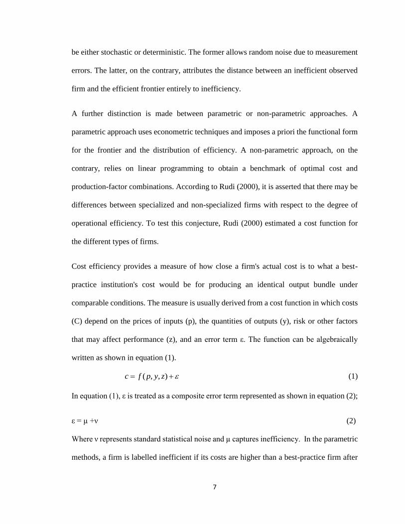
Cost efficiency provides a measure of how close a firm's actual cost is to what a best-
practice institution's cost would be for producing an identical output bundle under
comparable conditions. The measure is usually derived from a cost function in which costs
(C) depend on the prices of inputs (p), the quantities of outputs (y), risk or other factors
that may affect performance (z), and an error term ε. The function can be algebraically
written as shown in equation (1).
),,( zypfc (1)
In equation (1), ε is treated as a composite error term represented as shown in equation (2);
ε = µ +ν (2)
Where ν represents standard statistical noise and µ captures inefficiency. In the parametric
methods, a firm is labelled inefficient if its costs are higher than a best-practice firm after
8
removing random error. The methods differ in the way µ is disentangled from the
composite error term ε.
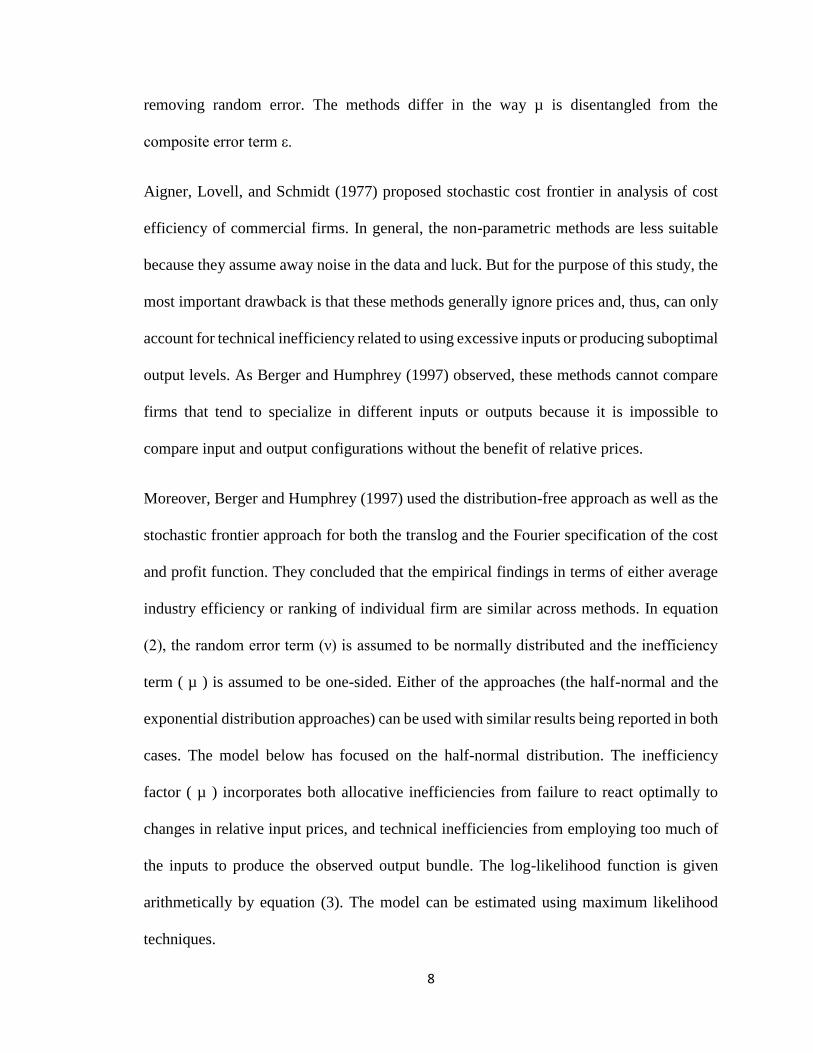
Aigner, Lovell, and Schmidt (1977) proposed stochastic cost frontier in analysis of cost
efficiency of commercial firms. In general, the non-parametric methods are less suitable
because they assume away noise in the data and luck. But for the purpose of this study, the
most important drawback is that these methods generally ignore prices and, thus, can only
account for technical inefficiency related to using excessive inputs or producing suboptimal
output levels. As Berger and Humphrey (1997) observed, these methods cannot compare
firms that tend to specialize in different inputs or outputs because it is impossible to
compare input and output configurations without the benefit of relative prices.
Moreover, Berger and Humphrey (1997) used the distribution-free approach as well as the
stochastic frontier approach for both the translog and the Fourier specification of the cost
and profit function. They concluded that the empirical findings in terms of either average
industry efficiency or ranking of individual firm are similar across methods. In equation
(2), the random error term (ν) is assumed to be normally distributed and the inefficiency
term ( µ ) is assumed to be one-sided. Either of the approaches (the half-normal and the
exponential distribution approaches) can be used with similar results being reported in both
cases. The model below has focused on the half-normal distribution. The inefficiency
factor ( µ ) incorporates both allocative inefficiencies from failure to react optimally to
changes in relative input prices, and technical inefficiencies from employing too much of
the inputs to produce the observed output bundle. The log-likelihood function is given
arithmetically by equation (3). The model can be estimated using maximum likelihood
techniques.
9
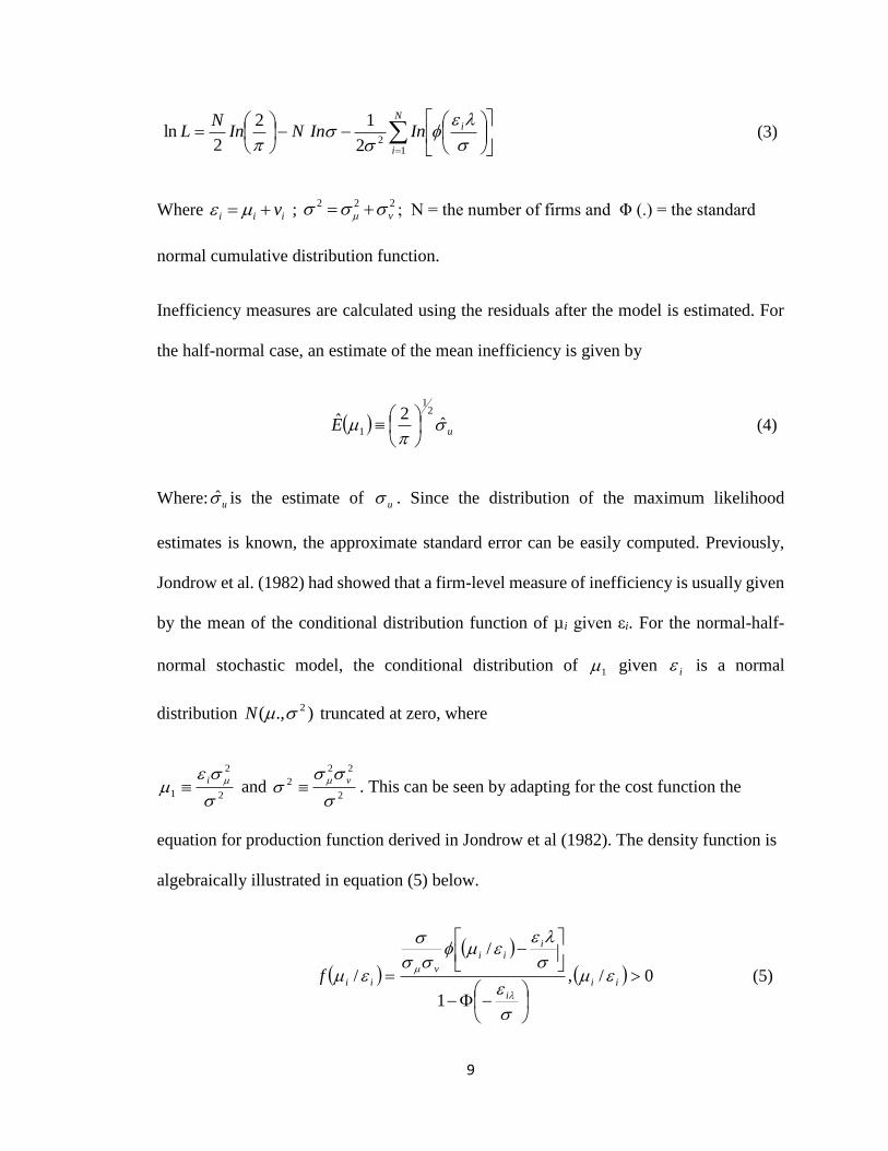
N
i
iInInNInN
L1
22
12
2ln
(3)
Where iii v ; 222
v ; N = the number of firms and Φ (.) = the standard
normal cumulative distribution function.
Inefficiency measures are calculated using the residuals after the model is estimated. For
the half-normal case, an estimate of the mean inefficiency is given by
uE
ˆ2ˆ
21
1
(4)
Where: u is the estimate of u . Since the distribution of the maximum likelihood
estimates is known, the approximate standard error can be easily computed. Previously,
Jondrow et al. (1982) had showed that a firm-level measure of inefficiency is usually given
by the mean of the conditional distribution function of µi given εi. For the normal-half-
normal stochastic model, the conditional distribution of 1 given i is a normal
distribution ).,( 2N truncated at zero, where
2
2
1
i and
2
22
2
v . This can be seen by adapting for the cost function the
equation for production function derived in Jondrow et al (1982). The density function is
algebraically illustrated in equation (5) below.
0/,
1
/
/
ii
i
i
ii
v
iif
(5)
10
The conditional mean iiE / is an unbiased but inconsistent estimator of µi since
regardless of the number of observations, the variance of the estimator remains non-zero.
Operational Efficiency
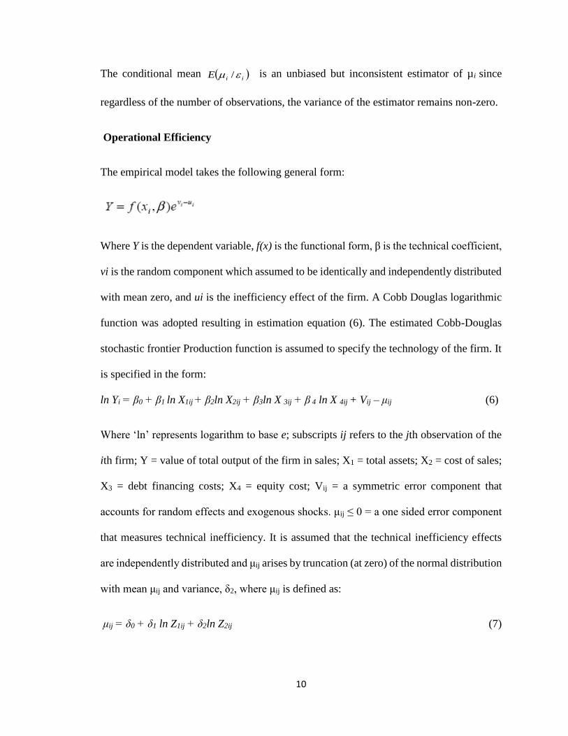
The empirical model takes the following general form:
Where Y is the dependent variable, f(x) is the functional form, β is the technical coefficient,
vi is the random component which assumed to be identically and independently distributed
with mean zero, and ui is the inefficiency effect of the firm. A Cobb Douglas logarithmic
function was adopted resulting in estimation equation (6). The estimated Cobb-Douglas
stochastic frontier Production function is assumed to specify the technology of the firm. It
is specified in the form:
ln Yi = β0 + β1 ln X1ij + β2ln X2ij + β3ln X 3ij + β 4 ln X 4ij + Vij – μij (6)
Where ‘ln’ represents logarithm to base e; subscripts ij refers to the jth observation of the
ith firm; Y = value of total output of the firm in sales; X1 = total assets; X2 = cost of sales;
X3 = debt financing costs; X4 = equity cost; Vij = a symmetric error component that
accounts for random effects and exogenous shocks. μij ≤ 0 = a one sided error component
that measures technical inefficiency. It is assumed that the technical inefficiency effects
are independently distributed and μij arises by truncation (at zero) of the normal distribution
with mean μij and variance, δ2, where μij is defined as:
μij = δ0 + δ1 ln Z1ij + δ2ln Z2ij (7)
11
Where μij represents the technical efficiency of the ith firm; Z1 = years of operation; and
Z2 = firm size; (Vi-Ui) = A composed error term where. Vij is the random error term
(statistical noise) and Ui: represents the technical inefficiency. The maximum–likelihood
estimates of the β and δ coefficients in equations (6) and (7), respectively was estimated
simultaneously using the computer program FRONTIER 4.1. The above model was used
for determining the efficiencies of firms in this study.
Profit Efficiency.
According to Rudi (2000), profit efficiency measures how close a firm comes to generating
the maximum obtainable profit given input prices and outputs. Berger and Mester (1997)
used the concept of alternative profit efficiency to relate profit to input prices and output
quantities instead of output prices. Alternative profit efficiency compares the ability of
firms to generate profits for the same level of outputs and thus reduces the scale bias that
might be present when output levels are allowed to vary freely. If customers are willing to
pay for high-quality services, the offering firms should be able to earn higher revenues that
compensate any excess expenditure and remain competitively viable.
In evaluating profit efficiency, the profit function uses essentially the same specification
as the cost function. The dependent variable is now ln(π + |πmin| + 1), where |πmin| is the
absolute value of the minimum value of π in the appropriate sample. In practice, the
constant term |πmin|+1 is added to every firm's profit so that the natural log is taken of a
positive number. This adjustment is necessary since a number of firms may exhibit
negative profits in the sample period. The dependent variable is ln (1)=0 for the firm with
the lowest value of π. π is calculated as all earnings minus interest and operating costs. The
explanatory variables remain unaltered. In this case, π is based on the output-mix
12
combining traditional and non-traditional firm activities. This produces a measure of profit
efficiency denoted by PE. A PE of 0.8 would mean that a firm is actually earning 80% of
best practice profits or that the firm is losing 20% of possible profits due to excessive costs,
deficient revenues, or both (Rudi, 2000).
1.1.4 Firm Value
The main goal of managing organizational funds is accomplishing the objective of wealth
maximization. Ehrhard and Bringham (2003) stated that the wealth of the business is
determined by the future cash flows' present value discounted using the company's WACC
(Linh, 2014). This means that WACC directly influences firm value (Johannes & Dhanraj,
2007). Market value can be used to measure the performance of publicly listed firms since
it requires information on the current stock prices.Additionally firm value considers all
future benefits to the firm, both short-term and long-term. This eliminates the problem of
estimating the time lag between implementation and increased profitability or productivity.
Other accounting ratios like the price to earnings ratio (P/E) ratio and market-to-book value
ratio suffer from a number of flaws in that accounting rules change, shifted reported
earnings without any real change in the underlying business. Further the large number of
accounting loopholes makes it easy for executives to mislead investors .Various evidence
based studies have used this market stock price to represent the firm value (Cheng &
Highes,2012, Boyd, 2010, Kakat, 2005, McConnel & Servaes, 1990)
Funds and a balance of sources of funding organization activities pre-determine attainment
of efficiency in using firm resources. This means that selecting appropriate risk and
economic environment for the company effectively reduces the cost of financing firm
investments and operations (Kohher, 2007). The value of a firm can be determined through
13
different methods but for the purpose of this study the value of the firm was obtained
through firm market share price.
1.1.5 Nairobi Securities Exchange
The Nairobi Securities Exchange (NSE) was constituted in 1954 as a cooperation of share
brokers registered under societies act with the mandate to develop and regulate trading
activities (Ngugi, 2003a). However, the Kenyan government has come up with many
reforms initiated towards the development of the stock market.
The key role played by the NSE is to promote a culture of savings whereby savers can
safely invest their money and consequently earn a return. NSE plays an important role of
facilitating the mobilization of capital for development through provision of an alternative
saving tool to the Kenyan savers. The money that was previous saved or spent was
redirected to investment projects in different economic sectors (NSE Hand Book, 2014).
This is an incentive to consume less and save more (NSE Hand Book, 2014). In July 2011
upon promulgation of constitution of Kenya 2010, the Nairobi Stocks Exchange Limited
rebranded to Nairobi Securities Exchange (NSE). As at December 2014 there were 62 firms
trading their shares at the NSE (NSE Hand Book, 2014). The NSE has a mandate to control
and manages stock and debt trading activities.
Effective management of the financing strategies is imperative to the firm financial success
and well-being hence the need for managers to manage their firm capital structure
carefully. A false decision on capital structure may lead to financial distress and, eventually
to bankruptcy (Donaldson’s, 1961). A continuing debate in corporate finance exists over
the question of how firms finance their investments and the effect of the financing

14
strategies on the firm value (Graham & Harvey, 2001).Performance of firms listed at the
NSE has been dismal to the extent that some have lately called for financial bailout. This
has been attributed to factors related to capital structure decision as well as other factors
within and outside the firm which could have adversely affected firm performance and
their market value (Lucy, Makau & Kosimbei, 2014; Kadongo et al., 2014). Some firms in
NSE have faced distressing situations following their dismal performance and have been
under constant pressure to not only deliver efficient quality services at minimal cost but
also improve their market value. For the last two decades there has been numerous reports
on mismanagement, maladministration and or financial irregularities reported in firms
listed at the NSE (Kinuu, 2014). A joint study by World Bank and KIPPRA, (2003) on
funding new investment projects of firms trading shares at the NSE noted that new
investments are mainly funded by use of short term financing and to some extent through
the bank loans including short term bank overdrafts. The study established that equity
financing contributed minimally suggesting that equity financing is not a popular
alternative amongst firms listed at the NSE.
1.2 Statement of the Problem
The link between capital structures of firms and their value have been considerably debated
(Draniceanu, 2013). The Modigliani and Miller theory of 1958 assumed a perfect market
with the key assumptions of information symmetry implying that in an ideal marketplace
context, the value of a firm is not dependent on how the firm is financed. This may not be
the case in practice since market imperfections emerge in form of taxes, information
asymmetry and other market inefficiencies causing variations in the value of the firm
(Draniceanu, 2013).

15
The debate on the influence of capital structure on the value of firm is inconclusive given
that empirical studies have yielded inconsistent results ranging from positive, negative to
no relationships at all. Holz (2002) noted that debt to equity ratio has a positive correlation
with business success or performance and value in terms of return to the owners of the firm
(ROE) and return on the assets owned by the firm (ROA). The results indicate that financial
managers effectively use borrowed funds to augment shareholders' earnings. The studies
by Abor (2005), Biekpe (2007) confirms the empirical results by Kadongo et al. (2014)
that capital structure cannot exhaustively explain the variations in firm value. This means
other variables such as macroeconomic environment and firm efficiency surface to
accelerate, decelerate or moderate the relationship between capital structures and firms
market value.
The review of the literature by Majumdar and Chibber (1997), Holz (2002), Dessi and
Robertson, (2003); Abor (2005), Abor and Biekpe (2007) and Kadongo et al., (2014) on
the relationship between capital structure firm value has provided mixed results that reveals
knowledge gaps and raises a fundamental question about the link between capital structure
and the value of firms listed at the Nairobi Securities Exchange.Additionally capital
structure concept has largely been studied in developing countries and understudied in
Kenya a developing country and at a level addressed by this study
The government of Kenya and the private sector have invested heavily in NSE to create an
enabling environment for doing business. While some firms listed at the NSE have
performed exceedingly well others have been experiencing declining performance despite
having the right capital structure combinations to an extent that some of the firms have
even been delisted from the NSE (NSE Hand Book, 2014). In the last decade (2005- 2014)
16
six firms (East Africa Packaging, African Tours and Hotels ltd, Eliots Bakery ltd, CMC
Holdings, Access Kenya, Tim Sales) were delisted due to poor performance. This was
mainly attributed to factors both within and outside the firm other than their capital
structure which could have negatively affected their performance and the resulting market
value. Their dismal performance did not only adversely affect their market value but also
shareholders wealth. Additionally global economic changes such as global economic
recession, fluctuation in oil prices, climate change and lately terrorism have adversely
affected economic environment for businesses in Kenya (NSE Hand Book, 2014).Further
the situation has been compounded by firm efficiency with regard to inefficiencies
emanating from mismanagement, maladministration and or financial irregularities which
militate against firm productivity and growth in firm market value (Letangule & Letting,
2012; Kinuu, 2014).
A number of methodological differences /gaps emerged between prio studies and the
current study. For example Holz (2002) used debt rations as a proxy for capital structure
and return on equity (ROE) and return on the assets (ROA) to measure firm performance
and value. Rayan (2008) used debt to equity ratio as proxy for capital structure and the firm
value was measured by use of Earnings per share, price Earnings ratio, Return on Equity,
Return on Assets, Earnings Value Added, and Operating profit Margin. Similarly
Kodongo, Mokoteli and Mwangi (2014) reviewed leverage against value of firms using
profitability and Tobin Q while Mwangi, Makau and Kosimbei (2014) used return on assets
(ROA) and return on equity (ROE) to measure firm performance. The above measures of
firm value can be manipulated by management and therefore fail to sufficiently measure
firm performance and value unlike market share price used in the current study which is
17
information driven (market perception value ) by factors related to firm’s financing
strategies, efficiencies and macroeconomic environment existed in the past and anticipated
into the future.
Further methodological difference between the above empirical studies and the current
study is that panel data scrutiny aided in assessing the extent to which the dependent
variable is a function of different independent variables in the current study. This is in
contrast with some of the previous studies which employed a simple pooled ordinary least
squares regression analysis methodology, thereby ignoring the time dimension of the data.
In situations where the panel data did not meet the assumption of regression analysis of no
autocorrelation, analysis was conducted by fitting a Prais Winsten Panel Regression model
which is robust for serial correlation. Likewise, corrected standard errors were utilized in
instances where the assumption of no heteroscedasticity was violated. Diagnostic testing,
which was largely ignored in previous studies, and the consequential remedial measures
helped the researcher to enhance the credibility of the results.
This study took cognizance of the fact firm value may be a function of factors key among
them capital structure. This means that other factors apart from financing influences the
firm performance and market value (Kandongo,Makoteli and Maina, 2014) The above
empirical studies on capital structure and firm value relationship did not identify nor
examine the influence of the macroeconomic environment and the linkage of firm
efficiency on the relationship between capital structure and firm value nor consider fitting
appropriate robust Panel Regression models in situations where normal panel regression
models did not fit the data sets of the firms floating their shares at the NSE.
18
This study sought to address these gaps by answering the research question: How does
macroeconomic environment and firm efficiency influence the link between capital
structure and value of firms whose shares are traded at NSE by use of panel data regression
analyses and in situations where the panel data sets did not meet the all the assumptions
of regression analysis, the panel data sets were analysed by fitting an appropriate robust
Panel Regression models.
1.3 Objectives of the Study
1.3.1 General Objective
The general objective of this research was to estabish the moderating and intervening
influence of macroeconomic environment and firm’s effeciency on the relationship
between capital structure and value of the firms listed at the NSE.
1.3.2 Specific Objectives
The specific objectives were to:
i) Establish the relationship between capital structure and the value of firms listed at
the NSE.
ii) Determine the moderating influence of macroeconomic environment on the
relationship between capital structure and value of firms listed at the NSE.
iii) Ascertain the intervening effect of firm efficiency on the relationship between
capital structure and value of firms listed at the NSE.
iv) To determine the joint effect of capital structure, macroeconomic environment and
firm efficiency on the value of firms listed at the NSE.
19
1.4 Value of the Study
This study is expected to add value into the existing knowledge in the areas of capital
structure, macroeconomic environment, firm efficiency and firm value in five main ways:
The first major contribution is the determination of the relevant factors that are important
in defining capital structure in firms listed in Nairobi Securities Exchange. Although
capital structure indicators (debt to equity ratio, retained earnings ratio, debt capital ratio
and equity capital ratio) are used to operationalize capital structure, experiences from
corporate sector indicate that Kenyan firms are relying more on equity capital than retained
earnings and debt. Thus the pecking order being equity, retained earnings and debt. This
study is meant to educate firm owners the importance of using retained earnings and
in the absence of retained earnings debt capital in order to benefit from tax shields
advantages to protect firm profit from heavy taxation in terms tax shields benefits.
Secondly, the study is envisaged to enhance building of existing theories by examining
theoretical propositions such as capital structure theories, transaction cost theory and
resources based theories whose key paradigm is the structural arrangement in aligning the
firm operations within the turbulent macroeconomic environment and internalize the ever
evolving firm efficiency in terms of efficiencies with both internal and external
environment in order to realize superior performance of their firms. Based on the forgoing,
firm managers should be able to reap the benefits from agency cost theory due to displinary
role of debts in their capital structure compositions which forces them to manage their firms
efficiencly from the point of view of operational efficiency, cost efficiency and profit
efficiency inorder to realise sufficient funds to pay off interest and outstanding debts
(principle). The strength of each of each measures of efficiencies should drive the firm
and significantly impact the overall value of the firm in the market .
20
Thirdly, the findings of this study are useful to various stakeholders including investors,
corporate managers, regulators and the government. The effects of capital structure on
firm value should help investors and corporate managers when financing their firm
investment and operations especially in the use of debt due to tax advantages embodied
in this form of financing when their firms are not able to retain funds from their profits,The
government through Capital Markets Authority (CMA) and other stakeholders in the
Kenyan corporate sector should develop appropriate policies in an attempt to organize
the debt capital market to enable Kenyan corporate bodies get access to low cost long
term debt capital to finance their investments and operations. It is imperative to develop
suitable trading regulations and mechanisms to augment the effectiveness of debt market
as optimal liquidity in secondary market reduces the cost of capital which positively
impacts in the value of Kenyan firms. Previous studies had revealed that Kenyan
firms relied more on costly equity finances instead of debt financing locking
themselves out of the tax shields benefits meant to enhance the value of the firms.
Fourthly, the outcome of this study enables the managerial practitioners to appreciate the
integration of the various financing methods in the face of turbulent macroeconomic
environment and ever evolving firm efficiency and correctly interpret the signals being
conveyed by these variables in order to generate the most rewarding values of their firms.
This involves leveraging their firm core processes with the latest technology which will
enable them benefits from efficiencies brought about by technological innovations. This
strategy will enable firm save on their costs which is very critical in generating enhanced
value of their firms.
21
Lastly, this study contributes in reducing the controversy on the relationship between
capital structure and firm value by showing that the relationship is not direct but is rather
moderated by macroeconomic environment and intervened by firm efficiency. This can
explain why many researchers who have tested the relationship between capital structure
and firm value have found contradictory results with some concluding the relationship
between the variables to be positive (Holz, 2002; Dessi& Robertson, 2003; and Kadongo
et al., 2014), negative (Majumdar& Chibber, 1997; Abor, 2005) or not significant (Abor&
Biekpe, 2007). This study provide fine grained directions that the linkage of capital
structure to the firm value can best be understood by considering how macroeconomic
environment and firm efficiency influence the relationship between capital structure and
firm value.
1.5 Organization of the Study
The first chapter offers background information, explains the research problem, the study
objectives, and the significance of the research. The second chapter highlights the
theoretical foundation that guide the relationship between the variables. Five theories that
is MM theory of capital structure, trade off theory, pecking order theory, agency theory
transaction cost theory and resource based theory are used to predict the expected
relationship amongst the research variables. Selected empirical models that guide the study
are included. The chapter ends with four main research hypotheses.
The third chapter highlights the framework that aided in reaching the research goals
including the data collection, their sources and how the variables were operationalized,
measured, and analysed. Chapter four presents the results of the data analysis, discusses
the descriptive statistics on capital structure, macroeconomic environment, firm efficiency
and value. Further diagnostic tests on the above variables which includes, tests for

22
multicollinearity, serial correlation, heteroscedasticity and panel level stationarity are also
discussed.
Chapter five presents the results of the tests of the four null hypotheses. The chapter
concludes with a discussion of the results of the hypothesis tested. Chapter six gives a
review of what was found out, conclusions of the study, contributions of the research
findings to knowledge, managerial policy and practice. The chapter further indicates the
limitations of the study and concludes with the suggestions for further studies.
23
CHAPTER TWO
LITERATURE REVIEW
2.1 Introduction
This chapter reviewed and critiqued the existing theoretical and empirical literature of the
study. Section 2.2 discusses the theoretical review of the study. Section 2.3 presents the
review of the empirical literature; Section 2.4 is the summary of the literature and
knowledge gaps Section 2.5 gives a conceptual framework of the study while section 2.6
presents a conceptual hypothesis.
2.2 Theoretical Review
Theoretical support for the study was drawn from the theories dealing with capital
structure, transaction costs and resources based theories. There are several theories that
explain the relationship between how firms are financed, managed and the resultant value.
They include Modigliani and Miller theory of capital structure (1958 & 1963) Transaction
Cost Theory (TCT) by Williamson (1985, 1998) Resource Based Theory (RBT) by Penrose
(1959), Pecking Order Theory by Myers and Majluf (1984), Trade-off model by Myers
(1984) and Agency Theory by Jensen and Meckling. MM theory of capital structure is the
anchoring theory in this study.
2.2.1 Modigliani and Miller Theory of Capital Structure
This theory as propounded by Modigliani and Miller states that if the capital markets are
perfect, an organization’s profitability has a larger impact on its value than capital structure
does, that is value irrelevant (Modigliani & Miller, 1958). The Modigliani and Miller
hypothesis is identical with the net operating income approach. At its heart, the theorem is
an irrelevance proposition, but the Modigliani-Miller Theorem provides conditions under
24
which a firm's financial decisions do not affect its value. They argue that in the absence of
taxes, a firm's market value and the cost of capital remain invariant to the capital structure
changes. In their 1958 articles, they provide analytically and logically consistent
behavioural justification in favour of their hypothesis and reject any other capital structure
theory as incorrect. The Modigliani-Miller theorem states that, in the absence of taxes,
bankruptcy costs, and asymmetric information, and in an efficient market, a company's
value is unaffected by how it is financed, regardless of whether the company's capital
consists of equities or debt, or a combination of these, or what the dividend policy is.
The Modigliani-Miller theorem can be best explained in terms of their proposition 1 and
proposition 2. However their propositions are based on certain assumption and particularly
relate to the behaviour of investors, capital market, the actions of the firm and the tax
environment. According to I.M Pandey (1999) the assumptions of the Modigliani - Miller
irrelevance proposition is based on
Perfect capital markets in which securities (shares and debt instrument) are traded in the
perfect capital market situation and complete information is available to all investors with
no cost to be paid. This also means that an investor is free to buy or sell securities, he can
borrow without restriction at the same terms as the firm do and behave rationally. It also
implies that the transaction cost (cost of buying and selling securities) do not exist.
Homogeneous risk classes in which firms can be grouped into homogeneous risk classes.
Firms would be considered to belong to a homogeneous risk class if their expected earnings
have identical risk efficiency. It is generally implied under the M-M hypothesis that firms
within same industry constitute a homogeneous risk class.The risk of the investors is
25
defined in terms of the variability of the net operating income (NOI). The risk of investors
depends on both the random fluctuations of the expected NOI and the possibility that the
actual value of the variable may turn out to be different than their best estimate.Further M-
M theorem assume that no corporate income taxes and personal tax exist. That is, they are
both perfect substitute and that firms distribute all net earnings to the shareholders, which
means a 100% payout.
In subsequent corrections, Modigliani and Miller (1963) established that when it is
possible to deduct interest expenses from the tax liability, the value of a firm increases as
the level of its leverage increases.With corporate income tax rate 𝑟𝑐,and 𝑝 on an after tax
basis, the equilibrium market value of levered firm is given by:
𝑉𝐿 = ��(𝐼 − 𝑟𝑐)/𝑝 + 𝑟𝑐𝐷𝐿
Where, X equals expected earnings before interest and taxes, ��(𝐼 − 𝑟𝑐)/𝑝 = 𝑉𝑢, value of
the firm if all-equity-financed, and 𝑟𝑐𝐷𝐿 is the present value of the interest tax-shield, the
tax advantage of debt. Given 𝑋, 𝑉𝐿 increases with the leverage, because interest is a tax-
exempt expense.This theory suffers from some limitations in that as the theory
successfully introduces the potential effects of corporate taxes into the theory, it only
leads to an extreme corner effect as the firm value is maximized when 100 per cent debt
finance is used (Mollik, 2008). Miller (1977) also showed that tax savings on interest
expenses are not certain, and the presence of personal taxes makes it difficult to derive
maximum benefit from using debt. De Angelo and Masulis (1980) also argued that tax
shields that accrue from non-debt sources introduce constrains on the benefits of using debt
to attain a tax advantage.
26
With respect to arbitrage process the principle that Proposition 1 is based on the assumption
that two firms are identical except for their capital structure which cannot command
different market value and have different cost of capital. Modigliani and Miller do not
accept the net income approach on the fact that two identical firms except for the degree of
leverage, have different market values. Arbitrage process will take place to enable investors
to engage in personal leverage to offset the corporate leverage and thus restoring
equilibrium in the market.
On the basis of the arbitrage process, M-M conclude that the market value of firms are not
affected by leverage but due to the existence of imperfections in the capital market,
arbitrage may fail to work and may give rise to differences between the market values of
levered and unlevered firms. Proposition 2 which incorporates arbitrage process may fail
to bring equilibrium in the capital market due to weaknesses in this proposition which
includes diferences in lending and borrowing which assumes that firms and individuals
can borrow and lend at the same rate of interest which does not hold in practice due to the
fact that firms which hold a substantial amount of fixed assets will have a higher credit
standing, hence they will be able to borrow at a lower rate of interest than individuals.The
proposition also assumes that personal leverage and corporate leverage are perfect
substitute which cannot hold in practice due to the fact that firms have limited liability
while individual have unlimited liability.For examples, if a levered firm goes bankrupt, all
investors will lose the amount of the purchase price of the shares. But if an investor creates
personal leverage, in the event of a unlevered firm's insolvency, he would lose not only his
principal in the shares but also be liable to return the amount of his personal loan.
27
On the other hand transaction cost interfere with the working of the arbitrage. Due to the
cost involved in the buying and selling of securities, it is necessary to invest a larger amount
in order to earn the same return. As a result, the levered firm will have a higher market
value. Further personal leverage are not feasible as a number of investors would not be able
to substitute personal leverage for corporate leverage and thus affecting the work of
arbitrage process.The proposition also ignores the corporate taxation and personal
taxation.and personal aspect of financing through retained earnings. In real world,
corporate will not pay out the entire earnings in the form of dividends and investors will
not show much interest in purchasing low rated shares by highly geared firm.
This study is anchored on the Modigliani and Miller (MM) theory of capital structure as
one of the theoretical underpinnings in explaining the link amid capital status of an
organization and firm value, the influence of macroeconomic environment and firm
efficiency are potential candidates to introduce market imperfections alongside other
associated costs influencing the relationship between capital structure and firm value.The
theory is important in the study as it sought to explain management of agency costs
through displinary role of debt capital in the firm’s capital structure and the influence
equity holders in the management of the company affairs through their representation in
the board of directors impacting in the generation of increased firm’s value.
2.2.2 The Pecking Order Theory
The theory was suggested by Myers and Majluf in 1984 and stated that businesses rank
their sources of funding operations and investments (from retained earnings to debt to
equity) such that equity gets the least preference. Hence, internal funds are used first, and
after their depletion, the issuance of debt follows. Firms only consider equity issuance

28
when it does not make sense to increase the level of debt. Key concepts of this theory
include the role of asymmetric information and transaction costs in shaping market
outcomes. Costs related to information asymmetry arise when a firm ignores external
funding and fails to invest in projects with positive NPV. The low preference for equity
results from perceptions of overvaluation among investors whenever managers consider
raising capital using equity. Myers and Majluf (1984) posit that the mispricing of equity
results from the wide deviation between the information possessed by investors regarding
the firm, and the true state of affairs. Some investors know that companies usually issue
new equity when the value of outstanding shares does not reflect the intrinsic level; this
knowledge causes the rational adjustment in the price that investors intend to pay for new
shares. Transaction costs comprise another premise of the pecking order theory. According
to Baskin (1989), firms prefer financing sources whose transaction costs are low;
consequently, debt gains preference as it attracts lower transaction costs than equity does.
By avoiding these external transaction costs the value of the firm is improved and sustained
over time. This alternative of short-term financing is disadvantageous in that the supplier
of this form of financing will charge higher interest rate as there is no security or collateral,
however the owners are assured of control of their firm, which is not diluted, by new
shareholders or owners.
Myers (1984) considers the lack of favourable combination of equity and debt as a logical
consequence of the pecking order theory. Changes in a firm debt ratio are proportional to
the level of its cash flows; as the cash flows increase, the debt ratio declines. The
application of the pecking order results into sets of costs, on one hand the increase
in the level of debts in the capital structure increases the likelihood of incurring
29
financial distress costs and in an effort to avoid this type of costs implies that the firm
will not be able to take up emerging projects that have positive NPV , this is a form of
opportunity costs . To mitigate this kind of costs firms with growth prospects will try to
avoid the depletion of the reserve capacity for borrowing in the short run.
2.2.3 The Trade-Off Model
Modigliani and Miller (1958) initially argued that firms maintain an optimal capital
structure, which strikes a delicate balance between the risk that a firm will go bankrupt and
the benefits resulting from tax-deductible interest expenses. The tax benefit of using debt
imply that for a firm to maximize its value, it must only use debt in funding investment
projects.However the existence of bankruptcy costs discourages firms from trading off
equity for debt (Brigham & Gapenski, 1996). Firms attain an optimal mix of debt and
equity when their marginal bankruptcy cost is at least as large as the marginal benefits that
result from the higher tax savings associated with using more debt. An efficient managerial
team should keep track of the evolution of the capital structure in order to establish whether
the firm has attained the optimal capital structure; after this, they should strive to ensure
the firm does not deviate from this optimum level. Simerly and Mingfang (2000)
established that the lack of a target for the optimal capital structure in firms stems from the
lack of adequate managerial incentives. Myers (1984) sees firms adopting the trade-off
model as those with a deliberate objective of containing the adverse impact of debt on firm
value. The undervaluation of equity in the market creates a disincentive for issuance of
equity, which creates undesirable perceptions among investors in the capital markets. The
difficulties in raising equity compound the attractiveness of debt as indicated by Miller
(1997); tax savings are seemingly large and predictable, whereas bankruptcy costs are not
30
substantial. Firms with a high level of profitability should have a markedly different
preference for debt compared to those with lower profits; highly profitable firms have
larger profits that they must shield from taxes. The static trade-off perspective equally
considers capital structure decisions as a balance of interest-tax-shield considerations
against the expenses resulting from financial distress. The variations in the efficiency of
firms in terms of efficiency lead to differences in the leverage ratio that firms aim to attain.
There are also differences in the nature of institutions, the financial systems, the rates of
taxation, and laws regulating bankruptcy processes; these differences have a profound
impact on the capital structure decisions. Where the value of intangible assets is high, the
firm faces a risk of losing them during the liquidation process. (De Angelo & Masulis,
1980). There must be a high level of reliance on the debt-servicing capacity to ensure that
there are adequate shields on a firm income against taxation translating to higher
profitability and market value for the firm.
2.2.4 Agency Theory
Jensen and Meckling (1976) developed the agency theory framework to highlight the
costs associated with the separation of the ownership and control of the firm. The conflict
between shareholders and managers can be resolved through the principals monitoring
the agents or offering them incentives in order for them to work in the best interest of the
principals. A key issue with the theory is that monitoring can be difficult to practically
execute and costs associated with the exercise can be non-trivial. Academicians, such as
Macho-Staedler and Perez-Castrillo (1997) have suggested that it might be less costly to
seek goal congruence between owners and managers. Attaining goal congruence between
owners and managers is also difficult especially due to the fact that self-interest may make
31
managers not fully disclose to the owners their true goals.
In proprietary ownership firms, the owners, managers and customers are three distinct
parties with checks and balances to reduce the likelihood of managers pursuing their
interests at the expense of the shareholders
The agency costs mentioned above do play a part in the determination of the ultimate value
of the firm depending on how the firm capital structure has been structured. Some agency
costs result from issuing equity; there are expenses of monitoring the activities of the agent
as well as paying the costs of the agent’s bonding expenses. The principal faces the
possibility of a reduction in welfare when the agent makes sub-optimal decisions. On the
other hand, issuing debt provides an incentive for investing in risky projects with high
returns, although there is a drastic increase in the risk of failure (Hansaker, 1999). Using
equity and debt attracts agency costs, making the optimal capital structure a balance of the
two sets of agency costs. The first set relates to committing a huge amount of a company's
earnings to the payment of interest and dividends which in a way helps in the management
of agency costs resulting from free cash flows. When we control for the degree to which a
business is profitable, a high level of leverage and low levels of dividend payout is
associated with high levels of investment. This is the same prediction offered in discussions
of incentives for controlling shareholders and bondholders when debt has a high risk,
investments fall below the conventional threshold and there are conflicts in substituting
assets (Fama & Miller, 1972; Jensen & Meckling, 1976; Myers, 1977). The anticipation of
inappropriate behaviour by the agent may prompt the debt holders to demand a premium
as a justification for the increase in the level of risk.

32
When wastages in free cash flow are controlled and the funds are directed towards
profitable firm investment, the firm will be appealing to the investors to bid for the
ownership of firm. To support this study motivation of value addition, the presence of debt
in the firm capital framework perform this role of directing firm free cash flow towards
profitable firm investment and this will create demand for the firm shares improving the
share price of the firm as evidenced by Fama and Miller (1972).
2.2.5 Transaction Cost Theory
This theory has become an increasingly useful framework for assessing how a variety of
issues are important to organizations (Williamson, 1985, 1998; Ghoshal & Moran, 1996;
Jones, 2004; Madhok, 2002). The TCT has included global business and strategic
management as areas of focus in deriving insights on the ways firms can enhance their
value.
Transaction cost theory is clear about the fact that firms can obtain economic outcomes
that are not efficient. An important premise of TCT is the qualitative aspect of the
differences between the incentives underlying hierarchies and those underlying the market.
These incentives can encourage actors to work together in cases where their absence would
create inefficient outcomes. Williamson (1985) argues that TCT’s main concern is the
dynamics of the organization of modern economic transactions.TCT considers the reasons
behind the internalization of some economic transactions inside a firm boundaries, whereas
others are placed under the responsibility of external parties. The general derivation is that
the internalization of activities within a firm boundaries results from market failures,
especially that of intermediate outputs. Transaction Costs Theory (TCT) argues that
transacting through the market creates costs that a firm can lower using different
33
mechanisms (Coase, 1937; Williamson, 1985). Williamson (1985) further notes that a firm
incurs a cost to draft, negotiate, and safeguard an economic transaction. According to the
TCT, the costs of an economic transaction are no less important than are those of producing
the actual output, and the assessment of operating costs is easier compared to the cost of
an economic transaction. In this study, transaction costs comprise an integral element of
all the costs incurred by a firm, which, has a bearing on the firm’s overall costs in terms of
production of goods and services. The efficiency with which this critical costs is managed
plays a fundamental role in the link between an organization’s capital structure and its
value in the market.
2.2.6 Resource Based Theory
This theory aids in comprehending the attainment of competitive advantage within a firm
and how it can upheld for a long period (Barney, 2001; Pearce, Robinson, & Mital, 2012).
This theory states that the different organizational resources greatly impacts on firm
productivity. Changes in organizational assets or resources will undoubtedly lead to
performance differences. Therefore, possession of resources which are unique is a source
of superior performance and increased value for the firm (Pasanen, 2013).
The RBT propositions arose from studies by Penrose (1959) and Chandler (1962). They
held a view that organizational success was dependent on company resources. RBT further
states that a successful business must have resources to use (Dollinger, 2003). This theory
is used to explain how the availability and efficient utilization of resources can create a
sustainable competitive advantage (SCA) and hence contribute to a firm value. Penrose
(1959) posited that the manner in which a firm deploys its resources can give it competitive
advantage over its competitors. This view was supported by Barney (1991) who contends
34
that firms that own resources which are rare, valuable, inimitable and non – substitutable
would attain a sustained competitive advantage. This theory posits that the
conceptualization of firms can take the form of a collection of resources, with the
distribution of resources across a firm occurring in a hetergenous manner; the differences
inherent in resources also tend to remain persistent (Amit&Schoemaker, 1993: Penrose,
1959; Wernerfelt, 1984). These assumptions have encouraged investigators to argue that
sustainable competitiveness results from the possession of resources that; have a high
value, are rare, and are difficult for competitors to imitate (Barney, 1995; Peteraf, 1993).
The extent to which resources are flexible influences the degree to which a firm can initiate
a successful response to changes in the external environment. Wiklund and Karlsson (1994)
have identified diverse forms of flexibility, including that of inputs, outputs, the internal
environment, and production networks. The nature of resources in a firm possession
constitutes its internal flexibility, e.g. flexibility of factors of production or the structure of
the firm.
Dyer and Singh (1998) argue that to the extent that a firm relates well with its external
environment, such as stakeholders, it has the capacity to respond well to external factors,
which constitutes competitive advantage. However, negative outcomes can result from the
dependency that network relations tend to create (Pfeiffer & Salancik, 1978). Barney
(1999) further argues that the decision on the kind of operating activities to undertake
within a firm, and those to outsource, is critical in the maintenance of competitiveness and
a strategic focus. The RBT’s growing influence has provoked research with some stating
that organizational assets greatly facilitate firm expansion (Talaja, 2012; Grant & Jordan,
2012). RBT continues to face challenges from scholars who hold that it has deficient
35
explanations and thus considered vague (Priem & Butter, 2001). These limitations
necessitate the need for evidence-based research on the variable and how this relates with
the concepts being studied (Ongeti, 2014).
2.3 Firm Value Measurement
Companies are owned by shareholders, the shareholders hire management to manage their
investments. One of key objectives of management is to maximize the shareholders returns
on their investment hence the essence of financial management is the creation of
shareholders wealth through enhanced value of the company's share prices. According to
Ehrhard and Bringham (2003), discounting at the weighted average cost of capital all the
cash flows that a business’ assets will generate in future gives its present value; the
assumption is that the business is operating as a going concern (Linh, 2014; Johannes &
Dhanraj, 2007).
Maximizing shareholder value requires financial, technical, human resources while
obtaining optimal maximum efficiency from these resources while selecting appropriate
risk for the company effectively reducing the cost of financing firm investments and
operations (Kohher, 2007). This implies that enhanced firm value can be realised through
application of value additive financing combinations within a framework of a favourable
macroeconomic environment and efficient appllicatin of firm resources in the generation
of superior firm market value.
The measures of firm value are basically returns to the firm assets and the owners of
the firm in the form of enhanced market price of firm shares. In order to achieve this
objective of enhanced firm market share price, the firm core processes and resources have
36
to be efficiently managed in a manner that optimal inputs are used to generate the desired
output. This can only happen if the macroeconomic environment is favourable (Isiki &
Hassan, 2002). The value measurement that are in line with the firm objectives are firm
optimal efficiency or inefficiency assessment, essentially measuring how well the firms
manages its resources in the process of maximizing shareholders wealth in terms of firm
earnings resulting to enhanced market price of the firm shares. Inefficiencies refer to how
a firm fails to attain the maximum output for a given set of inputs, or the failure to minimize
inputs for a particular set of outputs. Frontier analysis provides the means for measuring
firm efficiency linking to the enhancement of the firm value; it can be either parametric or
non-parametric. Through frontier analysis, it becomes possible to benchmark firm
effiencies to best practice firms as linkage to the value generation /performance of units
that make decisions. Berger and Mester (1997) argue that for frontier analysis to be
applicable, it is necessary to specify the inputs as well as outputs of a production process.
2.3.1 Parametric Approaches to Performance Measurement of Firms
Various parametric methodologies including stochastic frontier approach (SFA), the
deterministic frontier analysis (DFA) and the thick frontier approach (TFA) are adopted in
assessing organizational performance. In SFA, a function is specified; this function could
describe the costs, profits or production as they relate to input units, output units and
variables in the environment. The prediction of the output expectations is based on real
data about the inputs. Random error which increasingly follows a normal distribution-
constitutes the deviation of the output that the model predicts from what is actually
observed; the other component of this deviation is the inefficiency of the production
process, which take positive values and therefore have a half-normal distribution. Berger
37
and Humphrey (1997) argue that this approach is difficult to use because of the need for
the specification of production functions, besides the cumbersome task of separating
random errors and inefficiencies apart.
The deterministic frontier analysis equally approximates the input units and output units of
the production process; its procedures are similar to those of the SFA. DFA does not; unlike
SFA assume that errors in the model and inefficiencies in the production process can be
separated. Indeed it assumes the overtime, the model does not have error, and hence the
deviation between predictions and actual observations result from inefficient production
processes. There are no restrictions on the distribution of inefficiency as long as the
representative values are positive (Worthington, 2009). While TFA has the same
challenges as SFA and DFA do, it is not associated with the provision of estimates on how
a production process is efficient; instead, it offers a general view (Berger & Humphrey,
1997). When SFA and DFA are the only approaches available for analysing efficiency of
DMU SFA is preferable due to the fact that the approach takes advantage of little
industry knowledge required in order to determine good performers from others, or vise-
varsa (Beger & Humphrey, 1997: Worthington, 2009).
2.3.2 Non Parametric Approaches to Performance Measurement of Firms
The two major non-parametric frameworks include the data envelopment analysis (DEA)
and the free disposal hull (FDH). DEA entails the calculation of how efficient certain units
are, when compared to how similar units perform. It derives a ratio comprising the output
to which a weight has been attached, which is assessed in relation to the inputs that have
been weighted. Units with a high level of efficiency then make up the relative frontier,
which becomes the basis of evaluating whether other units are operating efficiently. The
38
designation of inputs and outputs is not constrained by specific rules. However, applying
the DEA requires one to identify input units and output units that are meaningful when
considered in the context of the DMUs under comparison. The DEA method determines
how a decision making unit is efficient through the maximization of how output units
compare to the input units, with the condition that a decision making unit should not have
a ratio larger than one, ultimately each DMU’s efficiency scores fall within the range of
zero and one. In the output –oriented method, the determination of efficiency scores
requires one to hold inputs units constant, and at the same time, examine the potential for
improvement in the outputs. The input–oriented DEA is not different from the approach
with an output orientation, save for the fact that the aim is to minimize how the input units
relate to the output units, subject to the constraint of ensuring that the ratios for every DMU
does not fall below one (Berger & Mester 1997; Berger & Humphrey, 1997). FDH is the
same as the DEA approach and constitutes a more general alternative of the DEA. Although
the DEA has an assumption of economic connectivity, the FDH fails to do so. It however
needs additional data for the significance and insightfulness of the outcome. In comparison
to DEA, FDH yields bigger estimations of efficiency; the two methods are frontier
approaches for establishing the highest level of technical efficiency (Berger & Humphrey
1997; Worthington, 2009).
2.3.3 Parametric Versus Non-Parametric Approaches
Non-parametric approaches generally show higher inefficiency levels than parametric ones
(Gual & Clemente, 1999). This is due to the fact that for each output /input combinations,
a DMU is compared with the best in the sample. The non –parametric approaches seek to
assess efficiency of a DMU relative to other firms in the same industry. It is therefore not
39
a requirement to define a production function. All deviations from efficient frontier are
assumed to be the result of inefficiency. However, the non-parametric approaches ignore
that some of the deviations from the efficient frontier could be the result of model
misspecification, or measurement error or environmental factors. This may result in
misstatement of inefficiency. A key advantage of the parametric approach like SFA is that
little industry knowledge is required in order to determine good performers from others, or
vise-varsa (Beger & Humphrey, 1997: Worthington, 2009).
The parametric approaches specify a production function and relates expected output to
various inputs. The difference between the actual output and the model predicted outputs
are attributed to model error or inefficiency. The greatest challenge to using the parametric
approach is the need to define a production function for the units being analysed. It is
difficult to determine the optimal combination of inputs that are required to produce given
outputs in an industry (Worthington, 2009).
This study applied the stochastic frontier technique/approach (SFT/A) to measure firm
efficiencies inorder to take care of deviations from the efficient frontier which could have
resulted from the model misspecification, or measurement error or environmental factors
leading to misstatement of inefficiency. Further the approach took advantage of little
industry knowledge required in order to determine good performers from others, or vise-
varsa (Beger & Humphrey, 1997: Worthington, 2009).Additionally the justification in the
use of SFA was also demonstrated by Aigner, Lovell, and Schmidt (1977), Berger and
Mester (1997b) and Fiorentino, Karmann, Koetter (2006).
40
Aigner, Lovell, and Schmidt (1977) proposed stochastic cost frontier in analysis of cost
efficiency of commercial banks. In general, the non-parametric methods are less suitable
because they assume away noise in the data and luck. But for the purpose of this study, the
most important drawback is that these methods generally ignored prices and, thus, can only
account for technical inefficiency related to using excessive inputs or producing suboptimal
output levels.
As Berger and Mester (1997b) observed, these methods cannot compare firms that tend to
specialize in different inputs or outputs because it is impossible to compare input and
output configurations without the benefit of relative prices. Moreover, Berger and Mester
(1997b) used the distribution-free approach as well as the stochastic frontier approach for
both the translog and the Fourier specification of the cost and profit function. They
concluded that the empirical findings in terms of either average industry efficiency or
ranking of individual bank are similar across methods.
Fiorentino, Karmann, Koetter (2006) investigated the consistency of efficiency scores
derived with two competing frontier methods in the financial economics literature namely:
Stochastic Frontier and Data Envelopment Analysis. They sampled 34,192 observations
for all German universal banks and analyzed whether efficiency measures yield consistent
results according to five criteria between 1993 and 2004: levels, rankings, identification of
extreme performers, stability over time and correlation to standard accounting-based
measures of performance. They found that non-parametric methods are particularly
sensitive to measurement error and outliers. Furthermore, their results showed that
accounting for systematic differences among commercial, cooperative and savings banks
is important to avoid misinterpretation about the status of efficiency of the total banking

41
sector.On the basis of the above justifications this study adopted Stachostic Frontier
Approach (SFA) to measure firm efficiency which prio studies by Nickell et al., 1997;
Nickell & Daphne, 1999 and Isiki & Hassan, 2002 had indicated to have a linkage to the
value of the firm .
2.4 Review of Empirical Literature
This part looks at the literature reviewed on the relationship between capital structure and
firm value, the moderating role of macroeconomic environment, the mediating influence
of firm efficiency and the joint effects of capital structure, macroeconomic environment
and firm efficiency on the value of the firm.
2.4.1 Capital Structure and Firm Value
The empirical literature review on the influence of capital structure on firm value has found
mixed findings ranging from positive by Holz (2002) who found that capital structure (debt
ratio) has a positive relation with financial outcomes in terms of return to the owners of
the firm (ROE) and return on the assets owned by the firm (ROA). The results suggest
the willingness of the managerial team to fund investment projects through borrowing, with
the proceeds of debt being applied in the maximization of firm performance and value.
Dessi and Robertson (2003) on the other hand found a positive impact of debt on the
performance and value of business enterprises.Dalbor et al. (2007) on the other hand
established that, keeping organizational size and risk constant, the return on assets of
lodging firms had a negative relation to their value, with capital expenditures lacking a
significant relation to the value of the firms.
42
Rayan (2008) found an inverse relation between the use of debt and value of the firms listed
at the Johannesburg Stock Exchange, with differences existing across various industries;
these findings were consistent with Hutchinson’s (1995) argument on the mediating role
of interest expenses in the link between capital structure and firm performance.
On the contrary, other studies found a negative relation in firm performance and value, that
capital structure related negatively with firm performance and value. Majumdar and
Chibber (1997) concluded that debt ratios in the firm capital structure inversely influence
firms’ performance and value; shareholders were restricted from paying dividends by the
creditors. Abor (2005) and Abor and Biekpe (2007) noted a negative and statistically
substantial effect of capital structure on value and performance of a business.
An investigation into the relationship between leverage, profitability and firm value of
listed firms in Kenya by Kodongo, Mokoteli and Mwangi (2014) using various panel
procedures found reasonably strong evidence that leverage significantly, and negatively
affected profitability of listed firms in Kenya. However, leverage has no effect on Tobin
Q, the proxy for firm value. Similar findings were reported by Mwangi, Makau and
Kosimbei (2014) in their investigation of the relationship between capital structures and
the performance of non-financial companies listed at the Nairobi Securities Exchange
(NSE). Their study employed an explanatory non-experimental research design using panel
data for the period 2007-2012. The study revealed that financial leverage had a statistically
significant negative relationship with performance as measured by return on assets (ROA)
and return on equity (ROE).Contrally Weill (2007) documented a positive impact of
financial leverage on Spanish and Italian firms, whereas German, French, and Belgian
companies experienced a negative impact from using debt.
43
The above empirical review considered either the influence of debt or equity on the value
of the firm and did not consinder the combined effects of debts and equity capital capital
on the value of the firms.
2.4.2 Capital Structure, Macroeconomic Environment and Firm Value
Previous empirical researches focused on capital structure and the value of the firm found
that firm value are not only influenced by capital structure choices but by firm other factors
both within and outside (Booth, Aivazia, Kunt & Makaimovi, 2001).
Fanelli and Keifman (2002) found that an unstable Argentinian macroeconomic
environment and external factors had a profound impact on the financial decisions of
business enterprises. They also argue that companies should only issue bonds when the
economic situation is ideal because during the given periods the firms are able to issue
bonds at favourable terms, which affects their earnings and market value of the firm shares.
Similarly, McConnell and Servaes (1995) in their study of the effect of macroeconomic
environment on the connection amid capital structure and company value concluded that
the influence of debt on firm value depended on the growth opportunities that are related
to the GDP growth rate of the country. The results of their study found that there was an
inverse relationship between the scope of growth opportunities and how debt is linked to
the value of a firm. Songshin and Adrian (2009) recommended that due consideration
should be given to external factors when making decisions on the optimal mix of debt and
equity; their research showed a negative relation between macroeconomic indicators and
the capital structure of European firms.
44
Cheng and Tzeng’s (2011) study revealed that Taiwanese firms with debt had a higher
value than those without debt; the financial quality of a firm played a considerable role in
mediating this relation. A similar study by Rao, Hamed, Al–yee and Syed (2007)
established an inverse relation between capital structure and the financial outcomes of the
operations of firms in Oman. Tax savings had little impact considering the costs of
borrowing funds in the Oman market, and the insufficient level of activities in the financial
markets.
The current study differs from empirical literature reviewed above by MaConnel and
Servaes,(1995) Fanelli and Keifman, (2002), Songshin and Adrian, (2008) and Cheng and
Tzeng’s ,(2011) in that these researches considered only two variables ,either the influence
of macroeconomic variables on the firm value or the influence of macroeconomic variables
on the firm value or the reverse , the researcher in this study considered the joint influence
of capital structure and macroeconomic variables on the value of the firms.
The above empirical literature considered pairwise relationship between either capital
structure and macroeconomic environment factors or between capital structure and the
value of firms.None of the studies reviewed considered the the moderating influence of the
macroeconomic environment on the relationship between capital structure and firm value
2.4.3 Capital Structure, Firm efficiency and Firm Value
Many studies on macroeconomic growth have demonstrated that gross country differences
in growth of GDP per capita are due to growth in total factor productivity (TFP) (Hall and
Jones, 1999; Easterly and Levine, 2001). Therefore, it is interesting to inquire whether
finance influences firm growth and market value through its impact on the efficiency of
45
the firm. This could be the case if the financial markets are able to supply capital to firms
and monitor them to achieve efficiency (Ayyagari, et al., 2007).
Several studies have examined the performance implications of efficiency measures and/
or efficiency changes using frontier analysis. Greene and Segal (2004) argue that “cost
inefficiency affects profits and growth through the negative effect of wasted resources on
earnings and cash flows.” This implies that more operationally efficient firms should be
more profitable. Greene and Segal, (2004) used SFA and documented a contemporary
association between profitability (ROE and ROA) and efficiency in the US life insurance
industry. Cummins and Xie (2008) on the other hand used DEA and indicated a positive
relation between firm efficiency and stock market reactions to acquisitions and divestitures
in the US property – liability insurance Industry.
Fenn, Drakos, Andrews and Knox (2008) conducted a more broadly research on efficiency
for a large sample of European manufacturing companies including food and chemicals
manufacturers. Their results show that efficiency scores and volatility of operational cost
and profit are meaningfully influenced by the size and market share of individual
companies. Noting that, most efficiency investigations in manufacturing industry are
focused on technical, allocative and cost efficiency.
Beccauli, Casu and Girardone, (2002) examined the relationship between estimated banks’
efficiencies and their share prices. They investigated the influence of X efficiency on the
share price of banks in five European markets in year 2000. Data Envelopment Analysis
(DEA) and Stochastic Frontier Analysis (SFA) have been applied to measure the cost
efficiency of banks by taking a sample of European Banks listed in the year 2000. Stock
46
performance of each bank has been regressed on early change of frontier change measures.
The results suggested that change in banks’ share price reflect percentage changes in cost
efficiency and the stocks of cost efficient banks tend to output their inefficient counterparts.
William and Segal (2004) examined the linkage of cost inefficiency and cross – sectional
variation in firm profitability in the US life insurance industry. Investigation has been made
on the relationship between organizational form, inefficiency in the life insurance industry
is substantial relative to profitability and that inefficiency is negatively associated with
profitability measures such as the return on equity. The analysis of inefficiency and
organizational form suggested that stock (shareholder – owned) companies. Additionally
Iommidis, Molyneux and Pasioura (2007) examined the relationship between bank
efficiency change and stock price returns. The impact of cost and profit efficiency on stock
return has been tested on a sample of 260 banks operating in 19 Asian and Latin American
countries between 2000 and 2006. The results represented appositive and robust
relationship between profit efficiency changes and stock returns has been applied. The
result revealed that profit efficiency netter explains bank stock returns compared to
traditional accounting profits measures (ROE) and profit efficiency measures include
useful information for shareholders wishing to explain bank stock returns.
Olena (2004) investigated the efficiency of Polish banks during the period of 1998-2000.
A Data Envelopment Analysis (DEA) methodology was applied which allowed for
distinguishing between five different types of efficiency namely: cost, allocative, technical,
pure technical, and scale. Additionally, Olena performed a number of parametric and non-
parametric tests to test whether foreign and domestic banks come from the same
population. Finally, univariate and multivariate regression analysis was employed in order
47
to detect the determinants of banking efficiency in Poland. The tests performed rejected
the null hypothesis that all banks come from the same population and thus all the results
were reported under the assumption of separate efficiency frontiers for foreign and
domestic banks. Over the study’s sample period, it was established that average efficiency
was 44.62% and 69.70% for domestic and foreign banks, respectively. Foreign banks
exhibited higher productivity of their inputs (technical efficiency) and were superior in
choosing the right mix of inputs in light of given prices (allocative efficiency). The study
concluded that foreign banks managed to utilize their comparative advantage and showed
a higher level of efficiency. This superiority should not be attributed to foreign ownership
per se. Instead, it is explained by better output quality, higher skilled personnel, and more
advanced technology. Thus, Olena (2004) added to the evidence that opening banking
markets to foreign capital fosters competition and adds to the efficiency of the banking
industry and market value of those banks.
Berger and Mester (1997a) studied the sources of differences in bank efficiency by
applying different efficiency concepts, different measurement methods, and different
potential correlates of efficiency to the same data set. They compared bank efficiency and
productivity change between the last six years of the 1980s and the first six years of the
1990s. Their data set included annual information from 1984 through 1995 on virtually all
U.S. commercial banks- totaling to over 145,000 annual bank observations in all. Their
findings suggested that each of three efficiency concepts -cost, standard profit, and
alternative profit efficiency - adds some independent informational value. The efficiency
results were remarkably robust to the different measurement techniques, different
functional forms, and various treatments of output quality used. Treatment of equity capital
was found to be an important consideration
48
Schumpeter (1934) studies on innovating firm production processes in United Kingdom
found businesses that are continually involved in creative and innovative practices are
predisposed to lasting success while those who do not, expose themselves to risk. Further
Artz, Norman, Hatfield and Cardinal, (2010) argued that increased competition and shorter
life cycles of products made innovation an integral issue for the performance of firms.
Similarly, in today’s intense competitive environment it is not surprising to find
technological innovations being a requisite objective for all firms and that there are
vulnerabilities from changes in the preferences of customers, augmented global rivalry and
shorter product lifecycles. Conventionally, all businesses ought to be innovative to boost
efficiencies despite their financing, industries and sizes inorder to enable the businesses
battle-out with other businesses and sustain their operations (Lipit , 2006 ). The empirical
results were also supported by Nickell et al (1997) and Nickell and Daphne (1999) who
observed a positive relationship between indebtedness and total factor productivity (TFP)
in the United Kingdom
However, other studies have reported a negative relationship between capital structure and
firm productivity. Pushner (1995) found negative effect of leverage on firm performance
measured as total factor productivity (TFP) in Japan. Booth et al (2001) in their study of
10 developing countries found a negative relation between leverage and firm performance
and firm value. Onaolapo and Kajola (2010) found a significant negative impact of
leverage on financial measures of firm performance in Nigeria.
There is a divergence of the studies reviewed above with the current study for example
Demerjian et al (2009) used a large sample of firms across industries and demonstrates that
managerial ability scores derived from DEA are positively and significantly associated
49
with current and past stock returns, executive compensation and investment opportunities.
Although the current study estimation method and the choice of output and input variables
are similar to those of Demerjian et al (2009), there are important differences between the
current study in that the current study performed a comprehensive examination of the
linkage of firm efficiency in terms of operations, cost and profit efficiencies on the
relationship between capital structure, and firm value that includes examining the
predictive power of changes in frontier analysis measures for changes in current and future
earnings per share and market share price, as well as examining whether investors and
analyst impound the predictive information to final market share price of the firm shares .
In contrast, Demerjian et al (2009) test whether efficiency is related to current and past
returns. Another important difference is that the current study used SFA in measuring firm
efficiency while Demerjian et al (2009) focused on DEA.
Further Demerjian et al (2009) used a levels design, while the current study used a changes
design. Using a changes design is important because it mitigates the potential issues of
endogeneity and correlated omitted variables and is consistent with prior research which
indicates that changes in efficiency are related to performances (Soliman,
2008).Additionally current study also differ in that, the researcher used a firm – level
measure of efficiency, while Demerjian et al (2009) used a manager – level measure of
efficiency. This is important because the current study is interested in how a firm
efficiency is related to performance and value, while Demerjian et al. (2009) were
interested in how CEO’s ability related to firm performance.

50
The above empirical literature considered pairwise relationship between either capital
structure and firm’s efficiency or between capital structure and the value of firms.None of
the studies reviewed considered the the intervening influence of the firm’s efficiency on
the relationship between capital structure and firm value
2.4.4 Capital Structure, Economic Environment, Firm efficiency and Value
The current studies hypothesis that capital structure, macroeconomic environment and firm
efficiency have a strategic impact and significantly contributes to firm value. Empirical
studies on capital structure and firm value have shown that there is a relationship between
the two. However, the direction of the relationships depended on the variables used by the
model hence the need to recognise the role being played by macroeconomic environment
and firm efficiency in the relationships.
However none of the studies have attempted to assess the joint effects of capital structure,
macro-economic environment, firm’s efficiency and firm value together but instead there
has been pairwise influence either between capital structure and firm value,
macroeconomic environment and firm value, firm efficiency and firm value or between
capital structure and firm efficiency or the reverse. This forms the gaps of this study
whereby the influence of capital structure, macroeconomic environment, firm efficiency
and value are assessed together.
2.5 Summary of Literature and the Knowledge Gaps
The empirical analysis of relationship between capital structure, macroeconomic
environment, firm efficiency, and firm value has yet to provide a convincing causal link
among these variables. A reasonable conclusion, based on the previous research, is that
capital structure matters in relation to firm value. It can also be concluded that capital
51
structure affects firm value through the debt component of capital structure due to tax
shield advantage which is meant to protect firm profit from taxation enhancing the firm
market value (Modigliani & Miller, 1958).
A number of conceptual, contextual and methodological research gaps arose from the
analysis of the issues examined in this chapter. The contextual gap arises from the fact that
capital structure concept has largely been studied in developing countries and understudied
in Kenya a developing country and at a level addressed by this study. The conceptual gaps
include lack of consensus and inconsistences on the influence of capital structure on the
value of the firms with some studies indicating positive and negative influences and others
no influence at all, making the study on the relationship between capital structure and firm
value inconclusive.
Another conceptual gap is that most studies on the firm value have not controlled for any
intervening or moderating variable. If variables such as the differences in firm efficiency
and macroeconomic environment are introduced in the model, then the link amid capital
status and organizational wealth may be different. This research introduces firm efficiency
with respect to operational, cost and profit efficiencies as an intervening variable and
macroeconomic environment with respect GDP growth, inlation and interest rate as a
moderating variable in an effort to explain further the association amid capital constitution
and firm value. A major limitation with most of the researches undertaken so far is that
they considered only two of the variables under study (capital structure, and firm value,
macroeconomic environment and firm value or firm efficiency, and firm value or the
reverse) at a time. No single research has considered the effects of the four variables taken
together. This study has tested whether capital structure, macroeconomic environment,
52
firm efficiency jointly have a significant influence on the wealth of businesses trading
shares at the NSE.
The methodological gap addressed by this study arises from the fact that traditional
financial analysis methods mainly used in the previous studies measured firm financial
performance and value using earnings per share, price earnings ratio, Return on
Equity(ROE), Return on Assets (ROA), Earnings Value Added (EVA), and Operating
profit Margin. The above measures of firm value can be manipulated by management and
therefore fail to sufficiently measure firm performance and value unlike market share
price used in the current study which is information driven (market perception value ) by
factors related to firm’s financing strategies, efficiencies and macroeconomic
environment existed in the past and anticipated into the future. Additional methodological
difference between the above empirical studies and the current study was that panel data
scrutiny aided in assessing the extent to which the dependent variable is a function of
different independent variables in the current study. This is in contrast with some of the
previous studies which employed a simple pooled ordinary least squares regression
analysis methodology, thereby ignoring the time dimension of the data. In situations where
the panel data did not meet the assumption of regression analysis of no autocorrelation,
analysis was conducted by fitting a Prais Winsten Panel Regression model which is robust
for serial correlation. Likewise, corrected standard errors were utilized in instances where
the assumption of no heteroscedasticity was violated. Diagnostic testing, which was largely
ignored in previous studies, and the consequential remedial measures helped the researcher
to enhance the credibility of the results.

53
Table 2.1 below is summary of the review of prior researches on the study variables of
capital structure, macroeconomic environment, firm efficiency and value of firms. For each
of the study the results, research gaps and how the current study addresses these gaps have
been shown.

54
Table 2.1: Summary of Literature and Knowledge Gaps
Empirical studies Design and
Focus
Methodology Findings Gaps Focus of current study
McConnell
&Servaes (1995)
Investigation of
influence of debt
on the firm value.
-Cross sectional survey
was used.
-Simple pooled ordinary
least regression analysis
was used
The influence of debt on
firm value depended on the
presence of growth
opportunities.
The study only used cross
sectional survey and ignored
time dimension of the data
.Additionally the study
considered only the internal
aspects of the relationship
between debt and firm
value.
The study used Panel data
regression analysis which
considered time dimension of the
data and considered the effects of
both internal and external factors of
the firm in the relationship between
capital structure and the firm value.
Majumdar &
Chibber (1997)
Investigated the
relationship
between capital
structure and
firm value.
-Cross sectional analysis
and two stage least square
(2SLS was used.
There was a negative
relationship between
capital structure and firm
value.
The study failed to consider
other interventions in the
relationship between capital
structure and the value of
the firm and used cross
section analysis method of
data analysis
The study considered the effect of
macroeconomic environment and
firm efficiency in the relationship
between firm leverage and value
and used Panell data regression
analysis which considered time
dimensions of the data
Kiogora (2000) Investigation of
the relationship
between returns of
firms quoted on
the NSE and their
level of leverage
-Cross sectional survey
was used simple pooled
ordinary least.
-Regression analysis was
used
There was a negative
relationship between the
returns and level of firm
leverage.
The study used cross section
survey method of data
analysis and failed to
consider other factors in the
relationship between firm
returns and leverage.
The current study used Panel data
regression analysis consindering
time dimension of the data
alongside the influence of
macroeconomic forces and effects
of firms’ efficiency in the
relationship between firm capital
structure and value.
Beccauli,Casu and
Girardone (2000)
Examination of
the relationship
between estimated
bank efficiency
and their share
prices in five
European markets
for year 2000
Cross sectional research
design was used to assess
the efficiency of
profitability on the value
of European banks in five
key markets by use of
Data Envelope Analysis
(DEA)
Change in banks share
price reflects percentage
change in cost efficiency,
and the stocks of cost
efficiency tend to output
their efficient counterparts.
The study considers data for
only one year hence it was
not possible to conduct
trend analysis of efficiency
measurement. Additionally
the study only considered
relative efficiency without
considering absolute
efficiency.
The current study considered a
period of six years for the purpose
of developing a trend analysis and
consinder time dimension of the
data in order to consider the effects
of profitability on firms share price.
Further the study used Stochastic
Frontier Analysis to measure the
efficiency of firm profitability on
value of the firm.
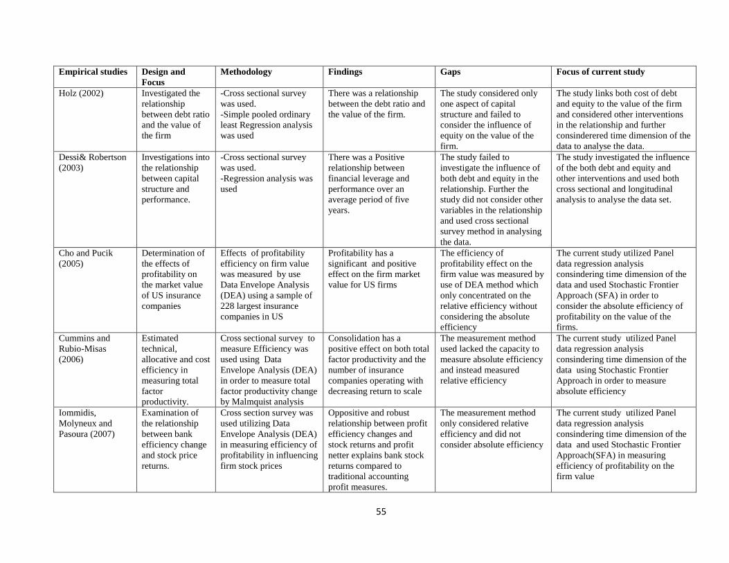
55
Empirical studies Design and
Focus
Methodology Findings Gaps Focus of current study
Holz (2002) Investigated the
relationship
between debt ratio
and the value of
the firm
-Cross sectional survey
was used.
-Simple pooled ordinary
least Regression analysis
was used
There was a relationship
between the debt ratio and
the value of the firm.
The study considered only
one aspect of capital
structure and failed to
consider the influence of
equity on the value of the
firm.
The study links both cost of debt
and equity to the value of the firm
and considered other interventions
in the relationship and further
consinderered time dimension of the
data to analyse the data.
Dessi& Robertson
(2003)
Investigations into
the relationship
between capital
structure and
performance.
-Cross sectional survey
was used.
-Regression analysis was
used
There was a Positive
relationship between
financial leverage and
performance over an
average period of five
years.
The study failed to
investigate the influence of
both debt and equity in the
relationship. Further the
study did not consider other
variables in the relationship
and used cross sectional
survey method in analysing
the data.
The study investigated the influence
of the both debt and equity and
other interventions and used both
cross sectional and longitudinal
analysis to analyse the data set.
Cho and Pucik
(2005)
Determination of
the effects of
profitability on
the market value
of US insurance
companies
Effects of profitability
efficiency on firm value
was measured by use
Data Envelope Analysis
(DEA) using a sample of
228 largest insurance
companies in US
Profitability has a
significant and positive
effect on the firm market
value for US firms
The efficiency of
profitability effect on the
firm value was measured by
use of DEA method which
only concentrated on the
relative efficiency without
considering the absolute
efficiency
The current study utilized Panel
data regression analysis
consindering time dimension of the
data and used Stochastic Frontier
Approach (SFA) in order to
consider the absolute efficiency of
profitability on the value of the
firms.
Cummins and
Rubio-Misas
(2006)
Estimated
technical,
allocative and cost
efficiency in
measuring total
factor
productivity.
Cross sectional survey to
measure Efficiency was
used using Data
Envelope Analysis (DEA)
in order to measure total
factor productivity change
by Malmquist analysis
Consolidation has a
positive effect on both total
factor productivity and the
number of insurance
companies operating with
decreasing return to scale
The measurement method
used lacked the capacity to
measure absolute efficiency
and instead measured
relative efficiency
The current study utilized Panel
data regression analysis
consindering time dimension of the
data using Stochastic Frontier
Approach in order to measure
absolute efficiency
Iommidis,
Molyneux and
Pasoura (2007)
Examination of
the relationship
between bank
efficiency change
and stock price
returns.
Cross section survey was
used utilizing Data
Envelope Analysis (DEA)
in measuring efficiency of
profitability in influencing
firm stock prices
Oppositive and robust
relationship between profit
efficiency changes and
stock returns and profit
netter explains bank stock
returns compared to
traditional accounting
profit measures.
The measurement method
only considered relative
efficiency and did not
consider absolute efficiency
The current study utilized Panel
data regression analysis
consindering time dimension of the
data and used Stochastic Frontier
Approach(SFA) in measuring
efficiency of profitability on the
firm value
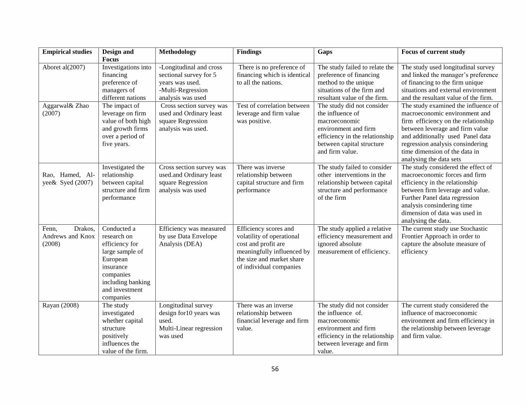
56
Empirical studies Design and
Focus
Methodology Findings Gaps Focus of current study
Aboret al(2007) Investigations into
financing
preference of
managers of
different nations
-Longitudinal and cross
sectional survey for 5
years was used.
-Multi-Regression
analysis was used
There is no preference of
financing which is identical
to all the nations.
The study failed to relate the
preference of financing
method to the unique
situations of the firm and
resultant value of the firm.
The study used longitudinal survey
and linked the manager’s preference
of financing to the firm unique
situations and external environment
and the resultant value of the firm.
Aggarwal& Zhao
(2007)
The impact of
leverage on firm
value of both high
and growth firms
over a period of
five years.
Cross section survey was
used and Ordinary least
square Regression
analysis was used.
Test of correlation between
leverage and firm value
was positive.
The study did not consider
the influence of
macroeconomic
environment and firm
efficiency in the relationship
between capital structure
and firm value.
The study examined the influence of
macroeconomic environment and
firm efficiency on the relationship
between leverage and firm value
and additionally used Panel data
regression analysis consindering
time dimension of the data in
analysing the data sets
Rao, Hamed, Al-
yee& Syed (2007)
Investigated the
relationship
between capital
structure and firm
performance
Cross section survey was
used.and Ordinary least
square Regression
analysis was used
There was inverse
relationship between
capital structure and firm
performance
The study failed to consider
other interventions in the
relationship between capital
structure and performance
of the firm
The study considered the effect of
macroeconomic forces and firm
efficiency in the relationship
between firm leverage and value.
Further Panel data regression
analysis consindering time
dimension of data was used in
analysing the data.
Fenn, Drakos,
Andrews and Knox
(2008)
Conducted a
research on
efficiency for
large sample of
European
insurance
companies
including banking
and investment
companies
Efficiency was measured
by use Data Envelope
Analysis (DEA)
Efficiency scores and
volatility of operational
cost and profit are
meaningfully influenced by
the size and market share
of individual companies
The study applied a relative
efficiency measurement and
ignored absolute
measurement of efficiency.
The current study use Stochastic
Frontier Approach in order to
capture the absolute measure of
efficiency
Rayan (2008) The study
investigated
whether capital
structure
positively
influences the
value of the firm.
Longitudinal survey
design for10 years was
used.
Multi-Linear regression
was used
There was an inverse
relationship between
financial leverage and firm
value.
The study did not consider
the influence of.
macroeconomic
environment and firm
efficiency in the relationship
between leverage and firm
value.
The current study considered the
influence of macroeconomic
environment and firm efficiency in
the relationship between leverage
and firm value.
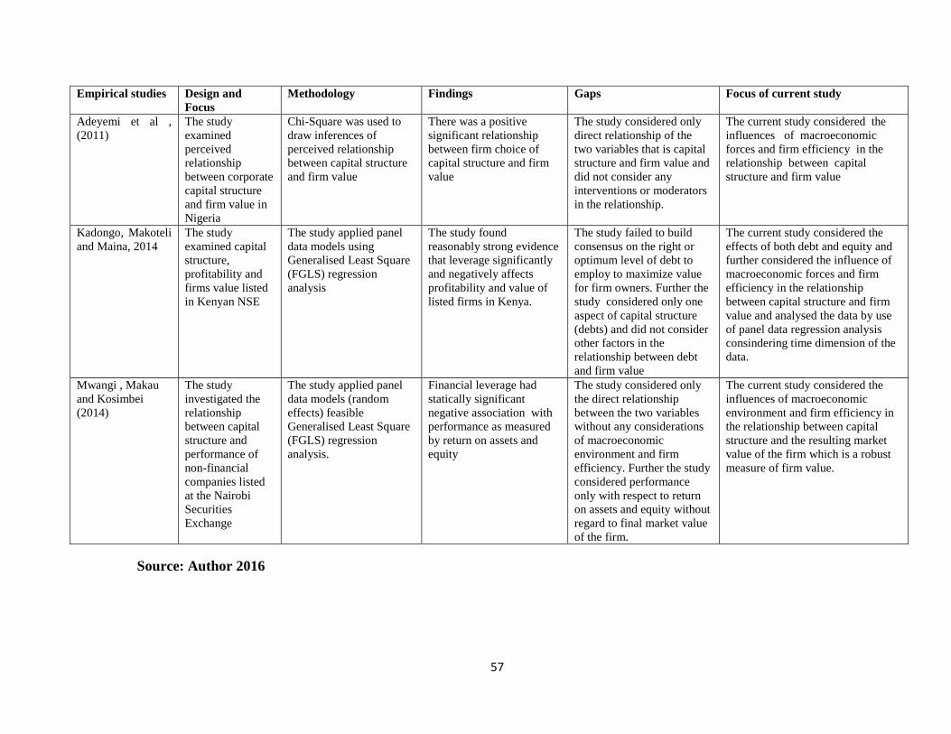
57
Empirical studies Design and
Focus
Methodology Findings Gaps Focus of current study
Adeyemi et al ,
(2011)
The study
examined
perceived
relationship
between corporate
capital structure
and firm value in
Nigeria
Chi-Square was used to
draw inferences of
perceived relationship
between capital structure
and firm value
There was a positive
significant relationship
between firm choice of
capital structure and firm
value
The study considered only
direct relationship of the
two variables that is capital
structure and firm value and
did not consider any
interventions or moderators
in the relationship.
The current study considered the
influences of macroeconomic
forces and firm efficiency in the
relationship between capital
structure and firm value
Kadongo, Makoteli
and Maina, 2014
The study
examined capital
structure,
profitability and
firms value listed
in Kenyan NSE
The study applied panel
data models using
Generalised Least Square
(FGLS) regression
analysis
The study found
reasonably strong evidence
that leverage significantly
and negatively affects
profitability and value of
listed firms in Kenya.
The study failed to build
consensus on the right or
optimum level of debt to
employ to maximize value
for firm owners. Further the
study considered only one
aspect of capital structure
(debts) and did not consider
other factors in the
relationship between debt
and firm value
The current study considered the
effects of both debt and equity and
further considered the influence of
macroeconomic forces and firm
efficiency in the relationship
between capital structure and firm
value and analysed the data by use
of panel data regression analysis
consindering time dimension of the
data.
Mwangi , Makau
and Kosimbei
(2014)
The study
investigated the
relationship
between capital
structure and
performance of
non-financial
companies listed
at the Nairobi
Securities
Exchange
The study applied panel
data models (random
effects) feasible
Generalised Least Square
(FGLS) regression
analysis.
Financial leverage had
statically significant
negative association with
performance as measured
by return on assets and
equity
The study considered only
the direct relationship
between the two variables
without any considerations
of macroeconomic
environment and firm
efficiency. Further the study
considered performance
only with respect to return
on assets and equity without
regard to final market value
of the firm.
The current study considered the
influences of macroeconomic
environment and firm efficiency in
the relationship between capital
structure and the resulting market
value of the firm which is a robust
measure of firm value.
Source: Author 2016
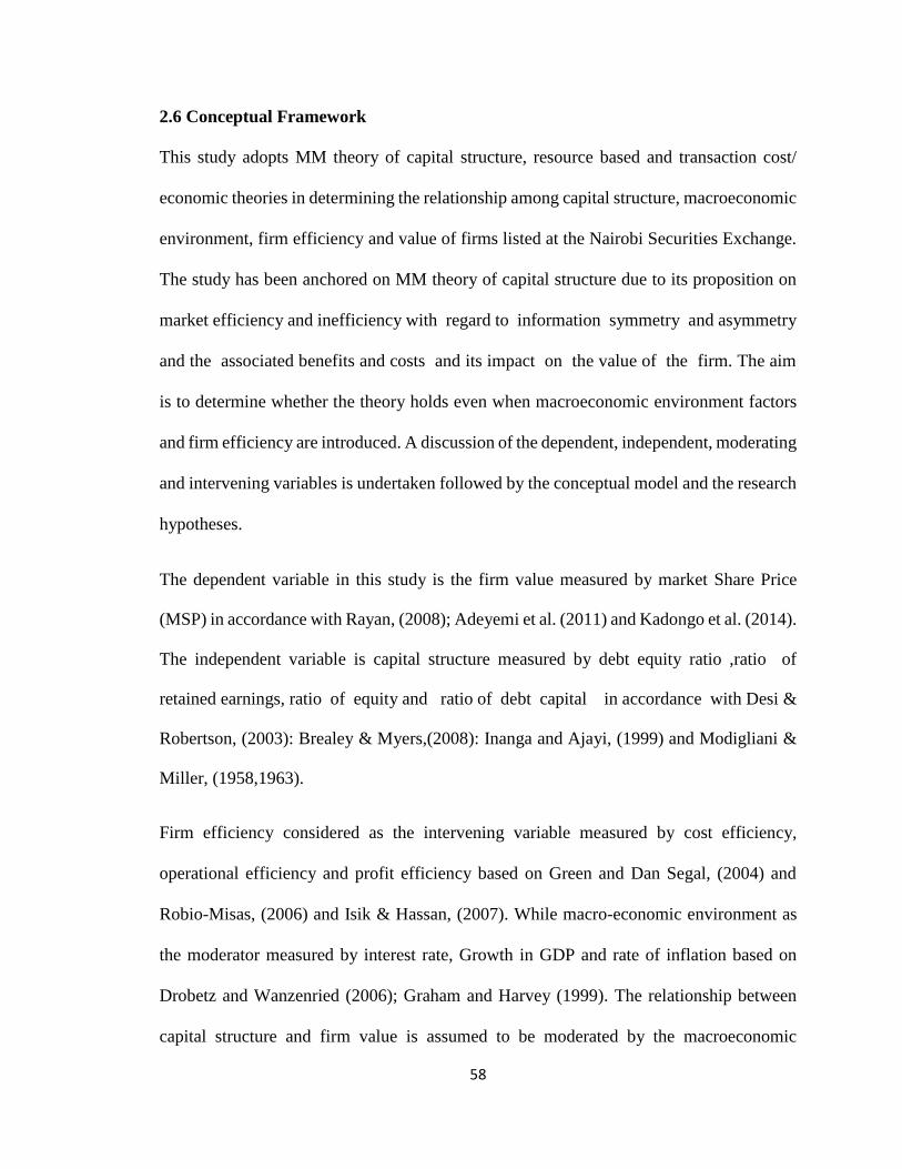
58
2.6 Conceptual Framework
This study adopts MM theory of capital structure, resource based and transaction cost/
economic theories in determining the relationship among capital structure, macroeconomic
environment, firm efficiency and value of firms listed at the Nairobi Securities Exchange.
The study has been anchored on MM theory of capital structure due to its proposition on
market efficiency and inefficiency with regard to information symmetry and asymmetry
and the associated benefits and costs and its impact on the value of the firm. The aim
is to determine whether the theory holds even when macroeconomic environment factors
and firm efficiency are introduced. A discussion of the dependent, independent, moderating
and intervening variables is undertaken followed by the conceptual model and the research
hypotheses.
The dependent variable in this study is the firm value measured by market Share Price
(MSP) in accordance with Rayan, (2008); Adeyemi et al. (2011) and Kadongo et al. (2014).
The independent variable is capital structure measured by debt equity ratio ,ratio of
retained earnings, ratio of equity and ratio of debt capital in accordance with Desi &
Robertson, (2003): Brealey & Myers,(2008): Inanga and Ajayi, (1999) and Modigliani &
Miller, (1958,1963).
Firm efficiency considered as the intervening variable measured by cost efficiency,
operational efficiency and profit efficiency based on Green and Dan Segal, (2004) and
Robio-Misas, (2006) and Isik & Hassan, (2007). While macro-economic environment as
the moderator measured by interest rate, Growth in GDP and rate of inflation based on
Drobetz and Wanzenried (2006); Graham and Harvey (1999). The relationship between
capital structure and firm value is assumed to be moderated by the macroeconomic
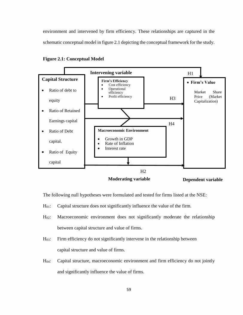
59
environment and intervened by firm efficiency. These relationships are captured in the
schematic conceptual model in figure 2.1 depicting the conceptual framework for the study.
Figure 2.1: Conceptual Model
The following null hypotheses were formulated and tested for firms listed at the NSE:
H01: Capital structure does not significantly influence the value of the firm.
H02: Macroeconomic environment does not significantly moderate the relationship
between capital structure and value of firms.
H03: Firm efficiency do not significantly intervene in the relationship between
capital structure and value of firms.
H04: Capital structure, macroeconomic environment and firm efficiency do not jointly
and significantly influence the value of firms.
DEPENDENT VARIABLES
Dependent variable Moderating variable
Intervening variable
H3
H4
H2
H1
Firm’s Value
Market Share
Price (Market
Capitalization)
Capital Structure
Ratio of debt to
equity
Ratio of Retained
Earnings capital
Ratio of Debt
capital.
Ratio of Equity
capital
Firm’s Efficiency Cost efficiency Operational
efficiency Profit efficiency
Macroeconomic Environment
Growth in GDP Rate of Inflation Interest rate
60
CHAPTER THREE
RESEARCH METHODOLOGY
3.1 Introduction
This section describes the activities that were adopted in executing the research. Section
3.2 presents the research philosophy while section 3.3 discusses the research model.
Section 3.4 presents the research's population; section 3.5 discusses the study sample while
section 3.6 discusses the data collection instruments. Section 3.7 discusses the diagnostic
tests which includes tests for multicollinearity, serial correlation, heteroscedasticity and
panel level stationarity. Section 3.8 discusses operationalization of research variables and
measurements while section 3.9 discusses data analysis concluding with data analysis
techniques.
3.2 Research Philosophy
Philosophy of science which is at the centre of knowledge development is pegged on
researcher's views or perceptions of what the world entails (Saunders, Lewis&
Thornbill,2007).There are two main research philosophies used in social science research,
namely Positivism and phenomenology. Positivism is based on use of statistical and
quantifiable computations of sampled variables to enhance formation of generalizations
about some variable (Johnson & Christensen, 2010). Positivism is premised on the
conjecture that the researcher is objective and thus independent of the variables being
investigated rather than being inferred subjectively (Mugenda & Mugenda, 2003). In
phenomenology the researcher does not only interact with what is being measured, reaches
conclusions through personalized assessment and interpretation of what he or she sees and
draws from them (Saunders et al., 2007).
61
Positivism is based on real facts, neutrality of the researcher, objective measurements of
the variables and validity of results. Saunders et al. (2007) pointed out that positivism
adopts a natural science stance where phenomena are objectively observed/measured
leading to production of credible data. This study is anchored on positivistic philosophy
because it sought to examine various theories. It equally sought to objectively establish
facts empirically and establish relationships among variables through statistical methods.
Hypothesis formulated in this study, were thus tested and confirmed or rejected through
statistical methods leading to recommendations as per the findings.
3.3 Research Design
Research design is the strategy or plan, used to acquire respondents. It also entails the
method of collecting data from them to draw conclusions about the study at hand (Zikmund
et al., 2010). There are three basic types of research design: exploratory, causal and
descriptive. Descriptive designs involve three main methods namely survey studies, the
correlation studies, and developmental studies (Cooper & Schindler, 2003). Descriptive
designs can also be categorized either as cross-sectional which involves drawing a sample
of elements from the population of interest and measuring efficiency of the elements only
once or longitudinal where sample members are measured repeatedly over time (Sekaran,
1992).
The study used descriptive and correlation longitudinal research design. A longitudinal
research is conducted over long time (could be decades). Descriptive longitudinal research
design is preferred where timescales are more generous. In this form of research, an aspect
is observed iteratively. The research entailed collecting published annual reports from
organization listed at the Nairobi Securities Exchange and were actively operational from
62
2009 to 2014. This period was chosen subject to data availability constraints. It also utilized
secondary data from the Nairobi Securities Exchange, Central Bank of Kenya (CBK),
Kenya National Bureau of Statistics (KNBS) NSE listed company’s reports and
handbooks. Reliability of data collected was enhanced by using audited financial annual
reports from selected organizations.
3.4 Population of the Study
The population for this research involved 62 companies listed on NSE between 2009 and
2014. The period was chosen as suitable as it offers current information as previous
researches by Mwangi, Makau and Kosimbei (2014) used data from year 2007 to 2012 and
the capital funding behaviour may have varied over the years.
3.5 Sample of the Study
The number of firm targeted for data analysis was 42 firms out of 62 companies quoted on
the NSE. Following the preceding research by Ozkan (2001), Flanery and Rangan (2006)
all the 20 companies in the financial segment were not included in the research as their
capital structures are highly regulated by various statutes and their financing structure is
different from non-financial institutions. The 20 firms entail insurance firms, banks, and
investment companies. There was no continuous data for Uchumi Supermarkets and
Hutchings Biemer Ltd since they were on suspension then. The two firms and another 10
firms where it was not possible to obtain data for six years were therefore excluded.
3.6 Data and Data Collection Instruments
The study collected secondary data from annual performance reports of the firms listed at
the Nairobi Securities Exchange. Additionally information on macroeconomic
environment in relation to interest, inflation and economic growth rates were extracted
63
from Nairobi Securities Exchange (NSE) Central Bank of Kenya (CBK) and Kenya
National Bureau of Statistics (KNBS) reports and hand books. The data extracted from
firms listed at the NSE included turnover, administrative costs, distribution costs, finance
costs, taxation costs, and profit after tax, number of equity shares, earnings per share,
market price of a share of firms listed at the Nairobi Securities Exchange for the period of
six years (2009-2014).
The study used data collection form (Appendix I) to collect the data. By taking a
longitudinal approach, the study measured how the identified problems are improved,
worsened or otherwise changed while determining the influence of macroeconomic
environment and firm efficiency on the relationship between capital structure and value of
the firms listed at the NSE. This is thus an indication of the accuracy of our prediction.
3.7 Diagnostic Testing
Diagnostic tests are pre estimation procedures that evaluate whether the assumptions of
Ordinary Least Squares (OLS) panel regression analysis are up held. In particular, a strong
linear relationship should not exist between any variables that are fitted jointly as regressors
in a model (no multicollinearity), there should be panel level stationarity, error terms
should be linearly independent (no autocorrelation), the variance of the error terms should
be constant (no heteroscedasticity), and the error terms should be normally distributed
(with a mean of zero and a constant variance). These assumptions and the particular tests
that were used to test for each of them are discussed in detail below.
64
3.7.1 Tests for Multicollinearity
The researcher used Variance inflation factors predictor variables to test multicollinearity.
Variance inflation factors (VIF) assesses the extent of variance of the estimated regression
coefficients relative to when these variables do not have a linear relationship.
3.7.2 Panel Level Stationarity
In order to analyze data using panel regression models, it should be stationary. Non
stationary data is likely to result in spurious regressions since mean and standard deviation
estimates derived from such data will be non-constant. To test the data for stationarity, the
Levin Lin Chu (LLC) Test unit root test was applied for all regression analyses of this
study. The null hypothesis being that panels contain unit roots, whereas the alternative
hypothesis implies stationarity in the panel data. Pertaining rejection criteria, the null
hypothesis of a unit root is rejected if the p value of the LLC test is less than 5%.
3.7.3 Serial Correlation
Serial correlation (also called autocorrelation) is a phenomenon which occurs when the
error terms of regression variables for successive periods are correlated. When present in
a dataset, it can distort the efficiency of regression estimators. Using the Wooldridge test
for serial correlation; we tested this study’s data for the presence of autocorrelation. The
null hypothesis for this test is that there is no first order autocorrelation in the panels and
is rejected if the p value of the test is less than 5%.
65
3.7.4 Likelihood Ratio Test for Heteroscedasticity
Heteroscedasticity is a serious problem since it tends to inflate the standard errors, thereby
increasing the probability of committing a type two errors, i.e. failing to reject a false
hypothesis about a coefficient. The Likelihood Ratio test was used to test the panel data for
heteroscedasticity. The null hypothesis of the Likelihood Ratio test is that the data is
homoscedastic across entities, i.e. the error terms have a constant variance. If the null is
rejected, the conclusion is that the data is heteroscedastic, i.e. the variance of error terms
across entities is not constant. The rejection criteria is that the null of homoscedasticity is
rejected if the p value of the Likelihood Ratio test is less than 5%.
3.7.5 Model Fitting
Classic panel data analysis suggests that the Hausman specification test should be used to
help the researcher in making a decision on whether to fit the random effects model or the
fixed effects model. These two models assume that the data meets all the assumptions of
regression analysis, i.e. no collinearity of regressors, no autocorrelation, and that the error
terms are normally distributed with a mean of 0 and a constant variance, i.e. no
heteroscedasticity. In instances where there are multicollinearity, the variable with the
highest Variance Inflation Factor (VIF) should be excluded from further analysis. In cases
of autocorrelation and heteroscedasticity, a Prais Winsten Panel Regression model should
be fitted. This is because this model is robust enough to generate plausible results in the
presence of these two violations of CLRM assumptions.
66
3.8 Operationalization of the Research Variables and Measurements
The independent variable of study (capital structure) was operationalized as the debt to
equity, ratio of retained earnings, debt capital and equity capital ratios as postulated by
(Desi & Robertson, 2003). Macroeconomic environment was operationalized as interest
rate, growth rate of GDP and inflation rate which is consistent with the study by (Cheng et
al., 2010).The intervening variable, firm efficiency, was operationalized as Cost efficiency,
operational efficiency and profit efficiency of the firm. This is consistent with the
operationalization of studies by (Diacon et al., 2002; Greene & Dan Segal, 2004; Cummins
& Rubio-Misas, 2006; Fenn et al., 2008). The dependent variable of this study, which is
firm value, was measured by market share price (MSP) (Rayan,2008);Adeyemi et al.,
2011;Kadongo et al.,2014). The study variables are operationalized as shown in Table 3.1
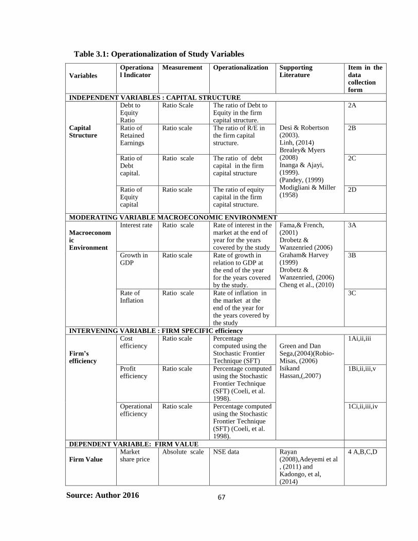
67
Table 3.1: Operationalization of Study Variables
Variables
Operational Indicator
Measurement Operationalization Supporting Literature
Item in the data collection form
INDEPENDENT VARIABLES : CAPITAL STRUCTURE
Capital Structure
Debt to Equity Ratio
Ratio Scale The ratio of Debt to Equity in the firm capital structure.
Desi & Robertson (2003). Linh, (2014) Brealey& Myers (2008) Inanga & Ajayi, (1999). (Pandey, (1999) Modigliani & Miller (1958)
2A
Ratio of Retained Earnings
Ratio scale The ratio of R/E in the firm capital structure.
2B
Ratio of Debt capital.
Ratio scale The ratio of debt capital in the firm capital structure
2C
Ratio of Equity capital
Ratio scale The ratio of equity capital in the firm capital structure.
2D
MODERATING VARIABLE MACROECONOMIC ENVIRONMENT
Macroeconomic Environment
Interest rate Ratio scale Rate of interest in the market at the end of year for the years covered by the study
Fama,& French, (2001) Drobetz & Wanzenried (2006) Graham& Harvey (1999) Drobetz & Wanzenried, (2006) Cheng et al., (2010)
3A
Growth in GDP
Ratio scale Rate of growth in relation to GDP at the end of the year for the years covered by the study.
3B
Rate of Inflation
Ratio scale Rate of inflation in the market at the end of the year for the years covered by the study
3C
INTERVENING VARIABLE : FIRM SPECIFIC efficiency
Firm’s efficiency
Cost efficiency
Ratio scale Percentage computed using the Stochastic Frontier Technique (SFT)
Green and Dan Sega,(2004)(Robio-Misas, (2006) Isikand Hassan,(,2007)
1Ai,ii,iii
Profit efficiency
Ratio scale Percentage computed using the Stochastic Frontier Technique (SFT) (Coeli, et al. 1998).
1Bi,ii,iii,v
Operational efficiency
Ratio scale Percentage computed using the Stochastic Frontier Technique (SFT) (Coeli, et al. 1998).
1Ci,ii,iii,iv
DEPENDENT VARIABLE: FIRM VALUE
Firm Value
Market share price
Absolute scale NSE data Rayan (2008),Adeyemi et al , (2011) and Kadongo, et al, (2014)
4 A,B,C,D
Source: Author 2016

68
3.9 Data Analysis
Data collected was analysed through combination of both descriptive and inferential
statistics. Panel data analyses were used to examine the extent to which the dependent
variable is a function of one or more of independent variables. This was considered to be
appropriate since it determines the influence of a single independent variable and several
independent variables on the dependent variable (Robson, 2002). The models used in the
study took the form below:
yit= α+ βxit+ λt + vit (1)
3.9.1 Data Analysis Techniques
Panel regression was adopted to ascertain the potency of the association amid dependent
and predictor variables; and the controlling effect of other factors. Different statistics were
derived from the analyses and interpreted in line with the studies' goals.
3.9.2 Empirical Model for Testing Hypothesis One: Effect of Capital Structure on
Firm Value
The first objective was to determine the relationship between capital structure and value
of firms listed at the Nairobi Securities Exchange. Dependent - independent variables
relationship model is:
FVit=β0+β1itDERit+β2itRERit+β3itERit+β4itDRit+it…………………………………(3.1)
Where:
FVit = Firm Value for ith firm in tth year.
β0= Intercept
β1it=Coefficient of Debt to Equity Ratio for ith firm in tth year.
DERit=Debt to Equity Ratio for ith firm in tth year.

69
β2it= Coefficient of Retained Earnings Ratio for ith firm in tth year.
RERit= Retained Earnings Ratio for ith firm in tth year.
β3it=Coefficient of Equity Ratio for ith firm in tth year.
ERit=Equity Ratio for ith firm in tth year.
Β4it=Coefficient of Debt Ratio for ith firm in tth year.
DRit=Debt Ratio for ith firm in tth year
it = Error Term
3.9.3 Empirical Models for Testing Hypothesis Two: Moderating Effect of
Macroeconomic Environment
Research objective number two was to establish the moderating effect of the
macroeconomic environment and the firm value. This was carried out using the two steps
methodology as in Stone-Romero & Liakhovitski (2002).The moderating effect was tested
in two steps whose model specifications are outlined below:
3.9.3.1 Step one of testing the Moderating Effect of Macroeconomic Environment
In step one, capital structure and macroeconomic environment were used in a panel
regression model as predictors of firm value. The empirical model that was tested in this
step is:
FVit = β0 + β1itDERit+ β2itRERit+β3itERit+β4itDRit + β5itGGRt+β6itINFRt+β7itINTRt+it.......(3.2)
Where:
FVit = Firm Value for ith firm in tth year.
β0= Intercept
β1it=Coefficient of Debt to Equity Ratio for ith firm in tth year.
DERit=Debt to Equity Ratio for ith firm in tth year.
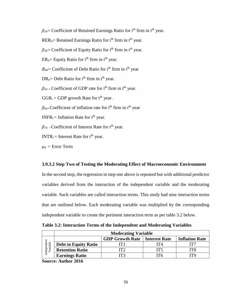
70
β2it= Coefficient of Retained Earnings Ratio for ith firm in tth year.
RERit= Retained Earnings Ratio for ith firm in tth year.
β3it= Coefficient of Equity Ratio for ith firm in tth year.
ERit= Equity Ratio for ith firm in tth year.
Β4it= Coefficient of Debt Ratio for ith firm in tth year
DRit= Debt Ratio for ith firm in tth year.
β5it = Coefficient of GDP rate for ith firm in tth year.
GGRt = GDP growth Rate for tth year.
β6it=Coefficient of inflation rate for ith firm in tth year
INFRt = Inflation Rate for tth year.
β7it =Coefficient of Interest Rate for tth year.
INTRt = Interest Rate for tth year.
it = Error Term
3.9.3.2 Step Two of Testing the Moderating Effect of Macroeconomic Environment
In the second step, the regression in step one above is repeated but with additional predictor
variables derived from the interaction of the independent variable and the moderating
variable. Such variables are called interaction terms. This study had nine interaction terms
that are outlined below. Each moderating variable was multiplied by the corresponding
independent variable to create the pertinent interaction term as per table 3.2 below.
Table 3.2: Interaction Terms of the Independent and Moderating Variables
Moderating Variable
Indep
end
ent
Var
iab
le GDP Growth Rate Interest Rate Inflation Rate
Debt to Equity Ratio IT1 IT4 IT7
Retention Ratio IT2 IT5 IT8
Earnings Ratio IT3 IT6 IT9
Source: Author 2016

71
In step two, the following model was fitted:
FVit = β0 + β1itDERit+ β2itRERit+β3itERit+ β4itGGRt+β5itINFRt+β6itINTRt+ λ1itIT1it+
λ2itIT2it+…. +λ12itIT12it +it ----------------------------------------------- (3.3)
Where:
FVit = Firm Value for ith firm in tth year.
β0= Intercept
β1it=Coefficient of Debt to Equity Ratio for ith firm in tth year.
DERit=Debt to Equity Ratio for ith firm in tth year.
β2it= Coefficient of Retained Earnings Ratio for ith firm in tth year.
RERit= Retained Earnings Ratio for ith firm in tth year.
β3it=Coefficient of Earnings Ratio for ith firm in tth year.
ERit= Equity Ratio for ith firm in tth year.
Β4it= Coefficient for GDP growth rate ith firm in tth year.
GGRt = GDP growth Rate for tth year.
Β5it= Coefficient for Inflation rate ith firm in tth year.
INFRt = Inflation Rate for tth year.
Β6it= Coefficient for Interest rate ith firm in tth year.
INTRt = Interest Rate for tth year.
λ1it…. Λ9it = Respective coefficients of the 9th interaction terms for ith firm in tth year.
IT1it…………IT9it = The 9th interaction terms for ith firm in tth year.
it = Error Term.
72
3.9.4 Empirical Models for testing Hypothesis Three: Intervening Effect of Firm’s
efficiency
The third research objective was to determine the intervening influence of firm efficiency
on the relationship between firm capital structure and the value of the firm. There were
four steps in testing the intervening effect of firm efficiency on the relationship between
capital structure and firm value. The pertinent models for the three steps are outlined below:
3.9.4.1 Step One of Testing the Intervening Effect of Firm’s efficiency
In step one, the model to be fitted was similar to model 3.1. As such, results of fitting
model 3.1 were considered. After fitting model 3.1, all regressors were significant and
hence they were considered further.
3.9.4.2 Step Two of Testing the Intervening Effect of Firm’s efficiency
Step two of testing the intervening effect of firm characteristic entailed estimating the
relationship between the capital structure and firm efficiency. Regression analysis was
done with the independent variables as the regressors of intervening variables. To prevent
the problem of multicollinearity, the variable “debt ratio” was excluded from further
analysis since it had a high degree of collinearity with the highest number of variables
(three)(r=0.878).Each intervening variable was estimated using the corresponding
independent variable, and the three panel regression models below were fitted:
CEFFit = β0 + β1itDERit +it…………………………………………………………(3.4)
OEFFit = β0 + β1itRERit +it…………………………………………………………(3.5)
PEFFit = β0 + β1itERit +it………………………………..…………………………(3.6)

73
Where:
CEFFit= Cost Efficiency for ith firm in tth year.
OEFFit= Operational Efficiency for ith firm in tth year.
PEFFit= Profit Efficiency for ith firm in tth year.
DERit=Debt to Equity Ratio for ith firm in tth year.
RERit= Retained Earnings Ratio for ith firm in tth year.
ERit= Equity Ratio for ith firm in tth year.
β0 = Intercept
β1it=Coefficient of the respective indicator of capital structure for ith firm in tth year.
it = Error Term
Only the variables whose coefficients are significant would be considered further. The
coefficients of all three independent variables of these equations were not significant. As
such, the researcher concluded that there is no intervening effect of firm efficiency at this
step. It was not possible to progress to step three and four.
3.9.5 Empirical Model for Testing Hypothesis Four: Joint Effect of Capital Structure,
Macroeconomic Environment, and Firm’s efficiency on Firm Value.
The fourth research objective was to establish the joint effect of firm capital structure,
macroeconomic environment and firm’s efficiency on the value of firms listed at the
Nairobi Securities Exchange.
The panel model that was used to test this hypothesis was:
FVit = β0 + β1itDERit+ β2itRERit+β3itERit+β4itDRit+β4itGGRt+β5itINFRt+β6itINTRt+
β7itCEFFit+ β8itOEFFit +β9itPEFFit+it ------------------------------------------------------ (3.3)

74
Where:
FVit = Firm Value for ith firm in tth year.
β0= Intercept
β1it=Coefficient of Debt to Equity Ratio for ith firm in tth year.
DERit=Debt to Equity Ratio for ith firm in tth year.
β2it= Coefficient of Retained Earnings Ratio for ith firm in tth year.
RERit= Retained Earnings Ratio for ith firm in tth year.
β3it=Coefficient of Equity Ratio for ith firm in tth year.
ERit=Equity Ratio for ith firm in tth year.
Β4 t = Coefficient of GDP growth Rate for tth year.
GGRt = GDP growth Rate for tth year.
Β5t = Coefficient of Inflation Rate for tth year.
INFRt = Inflation Rate for tth year.
Β6it = Coefficient of Interest Rate for tth year.
INTRt = Interest Rate for tth year.
Β7it = Coefficient of Cost Efficiency for ith firm in tth year.
CEFFit= Cost Efficiency for ith firm in tth year.
Β8it = Coefficient of Operational Efficiency for ith firm in tth year.
OEFFit= Operational Efficiency for ith firm in tth year.
Β9it = Coefficient of Profit Efficiency for ith firm in tth year.
PEFFit= Profit Efficiency for ith firm in tth year.
it = Error Term
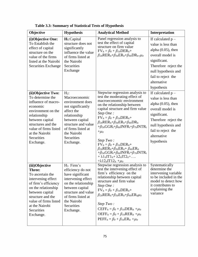
75
Table 3.3: Summary of Statistical Tests of Hypothesis
Objective Hypothesis Analytical Method Interpretation
(i)Objective One:
To Establish the
effect of capital
structure on the
value of the firms
listed at the Nairobi
Securities Exchange
H1:Capital
structure does not
significantly
influence the value
of firms listed at
the Nairobi
Securities
Exchange
Panel regression analysis to test the effect of capital structure on firm value FVit = β0 + β1itDERit+ β2itRERit+β3itERit+β4itDRit+it
If calculated p –
value is less than
alpha (0.05), then
overall model is
significant.
Therefore reject the
null hypothesis and
fail to reject the
alternative
hypothesis
(ii)Objective Two:
To determine the
influence of macro-
economic
environment on the
relationship
between capital
structures and the
value of firms listed
at the Nairobi
Securities
Exchange.
H2:
Macroeconomic
environment does
not significantly
affect the
relationship
between capital
structure and value
of firms listed at
the Nairobi
Securities
Exchange.
Stepwise regression analysis to test the moderating effect of macroeconomic environment on the relationship between capital structure and firm value Step One :
FVit = β0 + β1itDERit+
β2itRERit+β3itERit+β4itDRit
+β5itGGRt+β6itINFRt+β7itINTRt
+it
Step Two : FVit = β0 + β1itDERit+ β2itRERit+β3itERit+ β4itERit +β5itGGRt+β6itINFRt+β7itINTRt
+ λ1itIT1it+ λ2itIT2it+…. +λ12itIT12it +it
If calculated p –
value is less than
alpha (0.05), then
overall model is
significant.
Therefore reject the
null hypothesis and
fail to reject the
alternative
hypothesis
(iii)Objective
Three:
To ascertain the
intervening effect
of firm’s efficiency
on the relationship
between capital
structure and the
value of firms listed
at the Nairobi
Securities
Exchange.
H3 Firm’s
efficiency do not
have significant
intervening effect
on the relationship
between capital
structure and value
of firms listed at
the Nairobi
Securities
Exchange.
Stepwise regression analysis to test the intervening effect of firm’s efficiency on the relationship between capital structure and firm value Step One :
FVit = β0 + β1itDERit+
β2itRERit+β3itERit+β4itERitit
Step Two :
CEFFit = β0 + β1itDERit +it
OEFFit = β0 + β1itRERit +it
PEFFit = β0 + β1itERit +it
Systematically determine the intervening variable to be included in the model to detect how it contributes to explaining the variance
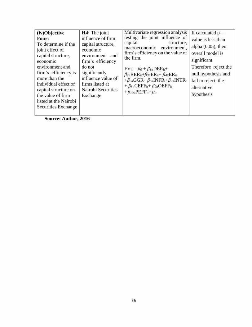
76
(iv)Objective
Four:
To determine if the
joint effect of
capital structure,
economic
environment and
firm’s efficiency is
more than the
individual effect of
capital structure on
the value of firm
listed at the Nairobi
Securities Exchange
H4: The joint
influence of firm
capital structure,
economic
environment and
firm’s efficiency
do not
significantly
influence value of
firms listed at
Nairobi Securities
Exchange
Multivariate regression analysis testing the joint influence of capital structure, macroeconomic environment, firm’s efficiency on the value of the firm. FVit = β0 + β1itDERit+
β2itRERit+β3itERit+ β4itERit
+β5itGGRt+β6itINFRt+β7itINTRt
+ β8itCEFFit+ β9itOEFFit
+β10itPEFFit+it
If calculated p –
value is less than
alpha (0.05), then
overall model is
significant.
Therefore reject the
null hypothesis and
fail to reject the
alternative
hypothesis
Source: Author, 2016
77
CHAPTER FOUR
DESCRIPTIVE DATA ANALYSIS AND PRESENTATION
4.1 Introduction
This section presents the results of the descriptive data analysis of the variables of the
study. It entails a discussion of the summary statistics of the study’s dependent variable
(market share price), independent variables (debt equity ratio, debt ratio, equity ratio, and
retained earnings), intervening variables (cost efficiency, operational efficiency, and profit
efficiency), and moderating variables (inflation rate, GDP growth rate and interest rate).
Unit root tests and correlation analysis are also presented for all variables.
4.2 Study Sample
Out of 42 non- financial institutions listed at the Nairobi Security Exchange that the study
initially targeted complete data was available for 30 companies. As such, the sample
consisted of 30 non-financial institutions that traded consistently over the 2009 to 2014
period and whose data was available. This represents a success rate of 71% that was
perceived as satisfactory. Munjuri (2013) conducted as study on insurance firms and
commercial banks and attained a success rate of 61% (54 out of 88). Machuki (2011)
achieved 43.3 % (23 out of 53) in a research of organizations floating their shares on the
NSE.
4.3 Research Design
The main objective of this study was to establish the nature of the association and the
influence of capital structure status on organizational wealth. The study further analysed
the impact of macroeconomic aspects and firm efficiency on the relationship between the
two main variables. This study employed a descriptive longitudinal research design. The
study used panel data analysis based on the generalized least squares model.
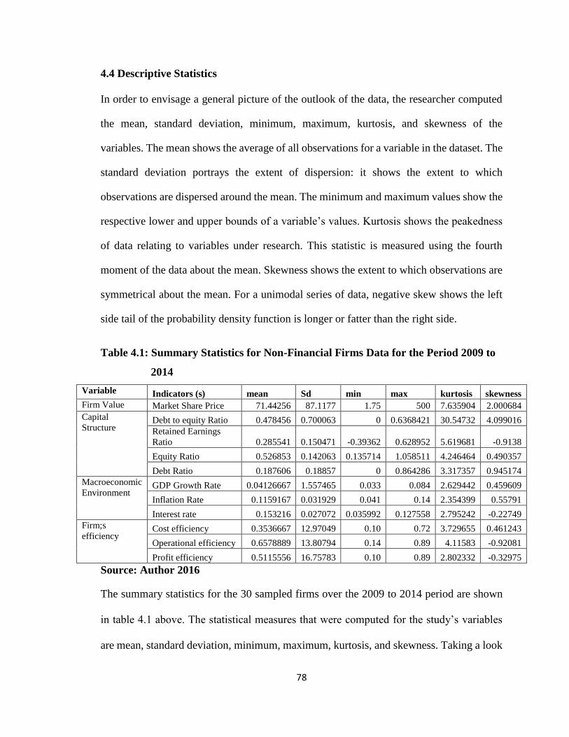
78
4.4 Descriptive Statistics
In order to envisage a general picture of the outlook of the data, the researcher computed
the mean, standard deviation, minimum, maximum, kurtosis, and skewness of the
variables. The mean shows the average of all observations for a variable in the dataset. The
standard deviation portrays the extent of dispersion: it shows the extent to which
observations are dispersed around the mean. The minimum and maximum values show the
respective lower and upper bounds of a variable’s values. Kurtosis shows the peakedness
of data relating to variables under research. This statistic is measured using the fourth
moment of the data about the mean. Skewness shows the extent to which observations are
symmetrical about the mean. For a unimodal series of data, negative skew shows the left
side tail of the probability density function is longer or fatter than the right side.
Table 4.1: Summary Statistics for Non-Financial Firms Data for the Period 2009 to
2014
Variable Indicators (s) mean Sd min max kurtosis skewness
Firm Value Market Share Price 71.44256 87.1177 1.75 500 7.635904 2.000684
Capital
Structure Debt to equity Ratio 0.478456 0.700063 0 0.6368421 30.54732 4.099016
Retained Earnings
Ratio 0.285541 0.150471 -0.39362 0.628952 5.619681 -0.9138
Equity Ratio 0.526853 0.142063 0.135714 1.058511 4.246464 0.490357
Debt Ratio 0.187606 0.18857 0 0.864286 3.317357 0.945174
Macroeconomic
Environment GDP Growth Rate 0.04126667 1.557465 0.033 0.084 2.629442 0.459609
Inflation Rate 0.1159167 0.031929 0.041 0.14 2.354399 0.55791
Interest rate 0.153216 0.027072 0.035992 0.127558 2.795242 -0.22749
Firm;s
efficiency Cost efficiency 0.3536667 12.97049 0.10 0.72 3.729655 0.461243
Operational efficiency 0.6578889 13.80794 0.14 0.89 4.11583 -0.92081
Profit efficiency 0.5115556 16.75783 0.10 0.89 2.802332 -0.32975
Source: Author 2016
The summary statistics for the 30 sampled firms over the 2009 to 2014 period are shown
in table 4.1 above. The statistical measures that were computed for the study’s variables
are mean, standard deviation, minimum, maximum, kurtosis, and skewness. Taking a look

79
at the statistics for the dependent variable, market share prices of the sampled firms,
analysis indicate that the share prices were quite volatile across the panels, with a low of
Kshs 1.75 and a high of Kshs 500. The mean of market share price was Kshs 71.44256.
Additionally, this variable had a kurtosis of 7. 635904 and a skewness of 2.000684 this
implies that the market share prices had fat tails, a leptokurtic distribution, and right
skewness.
The debt to equity ratio variable had a mean of 0.478456, which essentially means that on
average, the firms had 48 cents in debt for every shilling of equity in their balance sheet.
With a standard deviation of 0.7, it is evident that debt to equity ratios of the sampled firms
were quite dispersed. This is affirmed further by the fact that the minimum value for debt
to equity was 0 (i.e. 100% equity financing) while the maximum value was 6.368421 (i.e
these firm were extremely leveraged during the pertinent period. It held Kshs 6.36 in debt
for each 1Kshs it had in equity). The debt to equity exhibited a very high level of kurtosis
(30.54732) and positive skewness (4.099016).
Observations for the retained earnings ratio showed that on average, 28.55% of the assets
of the sampled firms were financed using retained earnings. The least value for this statistic
was -0.39362 (implying a loss making situation) while the highest value was 0.628952.
Just like other variables, the retained earnings ratio had a leptokurtic distribution
(kurtosis=5.619681) but in contrast with other variables, retained earnings ratio had a
slightly negative skewness (-0.9138)
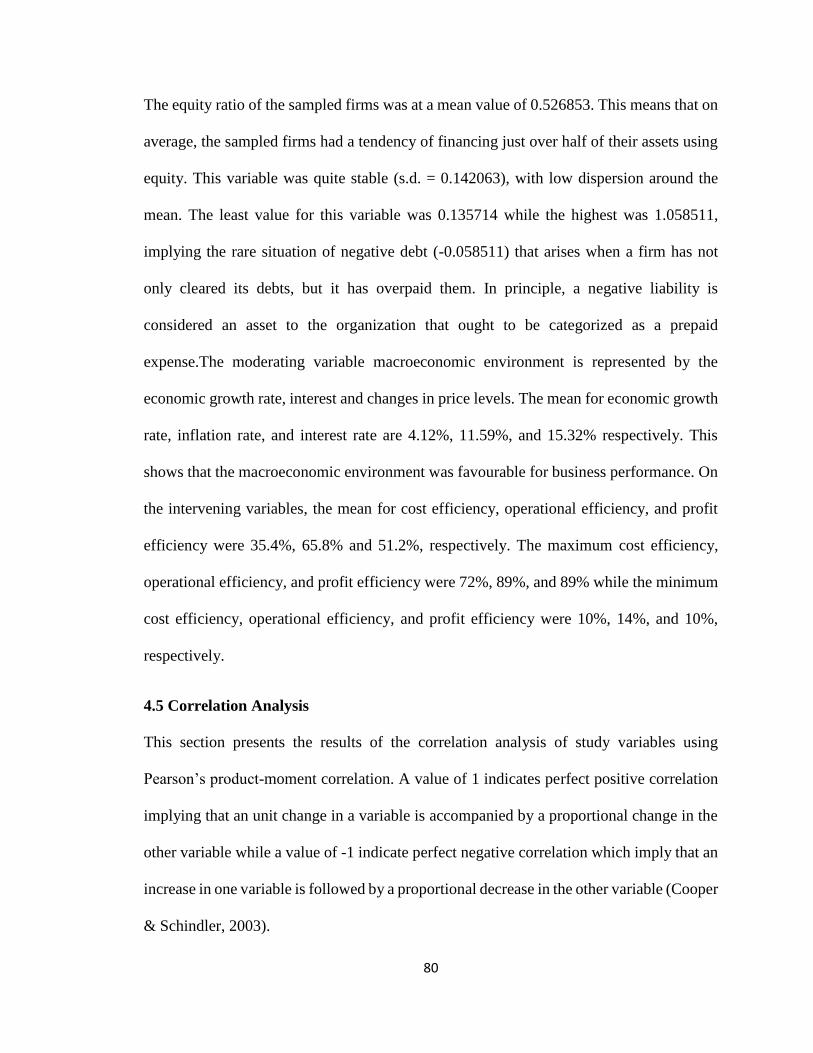
80
The equity ratio of the sampled firms was at a mean value of 0.526853. This means that on
average, the sampled firms had a tendency of financing just over half of their assets using
equity. This variable was quite stable (s.d. = 0.142063), with low dispersion around the
mean. The least value for this variable was 0.135714 while the highest was 1.058511,
implying the rare situation of negative debt (-0.058511) that arises when a firm has not
only cleared its debts, but it has overpaid them. In principle, a negative liability is
considered an asset to the organization that ought to be categorized as a prepaid
expense.The moderating variable macroeconomic environment is represented by the
economic growth rate, interest and changes in price levels. The mean for economic growth
rate, inflation rate, and interest rate are 4.12%, 11.59%, and 15.32% respectively. This
shows that the macroeconomic environment was favourable for business performance. On
the intervening variables, the mean for cost efficiency, operational efficiency, and profit
efficiency were 35.4%, 65.8% and 51.2%, respectively. The maximum cost efficiency,
operational efficiency, and profit efficiency were 72%, 89%, and 89% while the minimum
cost efficiency, operational efficiency, and profit efficiency were 10%, 14%, and 10%,
respectively.
4.5 Correlation Analysis
This section presents the results of the correlation analysis of study variables using
Pearson’s product-moment correlation. A value of 1 indicates perfect positive correlation
implying that an unit change in a variable is accompanied by a proportional change in the
other variable while a value of -1 indicate perfect negative correlation which imply that an
increase in one variable is followed by a proportional decrease in the other variable (Cooper
& Schindler, 2003).
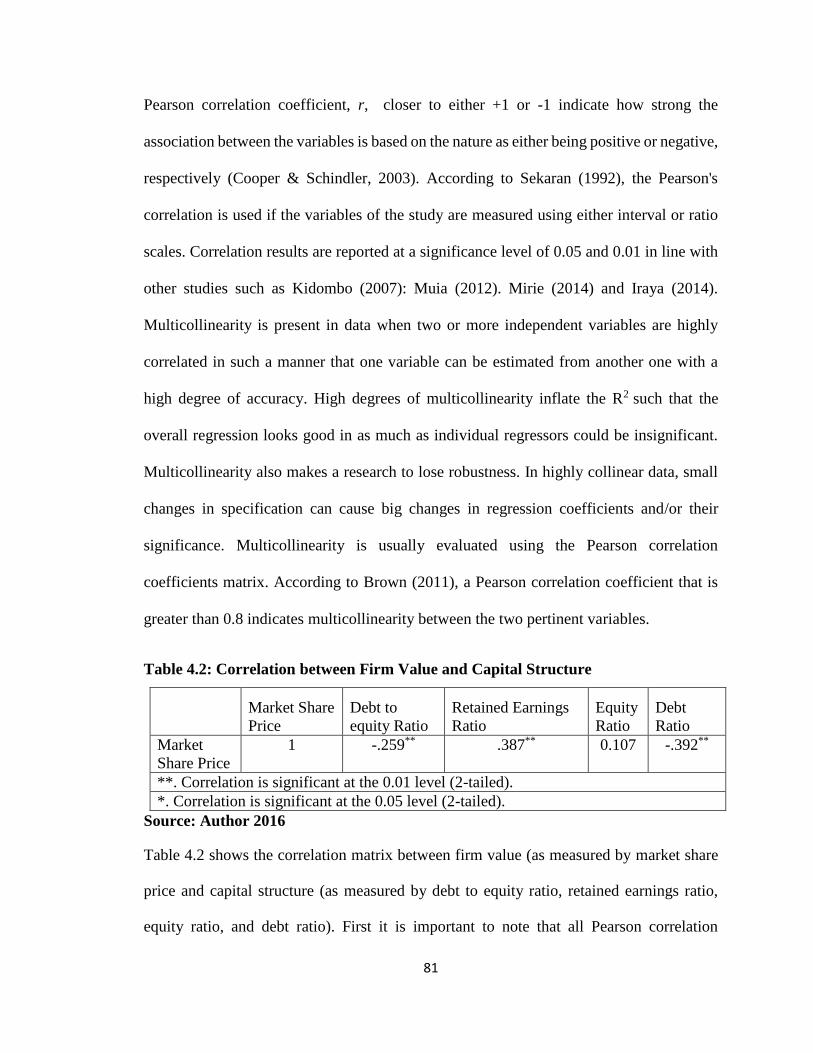
81
Pearson correlation coefficient, r, closer to either +1 or -1 indicate how strong the
association between the variables is based on the nature as either being positive or negative,
respectively (Cooper & Schindler, 2003). According to Sekaran (1992), the Pearson's
correlation is used if the variables of the study are measured using either interval or ratio
scales. Correlation results are reported at a significance level of 0.05 and 0.01 in line with
other studies such as Kidombo (2007): Muia (2012). Mirie (2014) and Iraya (2014).
Multicollinearity is present in data when two or more independent variables are highly
correlated in such a manner that one variable can be estimated from another one with a
high degree of accuracy. High degrees of multicollinearity inflate the R2 such that the
overall regression looks good in as much as individual regressors could be insignificant.
Multicollinearity also makes a research to lose robustness. In highly collinear data, small
changes in specification can cause big changes in regression coefficients and/or their
significance. Multicollinearity is usually evaluated using the Pearson correlation
coefficients matrix. According to Brown (2011), a Pearson correlation coefficient that is
greater than 0.8 indicates multicollinearity between the two pertinent variables.
Table 4.2: Correlation between Firm Value and Capital Structure
Market Share
Price
Debt to
equity Ratio
Retained Earnings
Ratio
Equity
Ratio
Debt
Ratio
Market
Share Price
1 -.259** .387** 0.107 -.392**
**. Correlation is significant at the 0.01 level (2-tailed).
*. Correlation is significant at the 0.05 level (2-tailed).
Source: Author 2016
Table 4.2 shows the correlation matrix between firm value (as measured by market share
price and capital structure (as measured by debt to equity ratio, retained earnings ratio,
equity ratio, and debt ratio). First it is important to note that all Pearson correlation
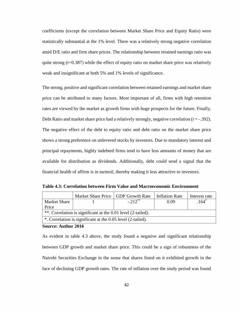
82
coefficients (except the correlation between Market Share Price and Equity Ratio) were
statistically substantial at the 1% level. There was a relatively strong negative correlation
amid D/E ratio and firm share prices. The relationship between retained earnings ratio was
quite strong (r=0.387) while the effect of equity ratio on market share price was relatively
weak and insignificant at both 5% and 1% levels of significance.
The strong, positive and significant correlation between retained earnings and market share
price can be attributed to many factors. Most important of all, firms with high retention
rates are viewed by the market as growth firms with huge prospects for the future. Finally,
Debt Ratio and market share price had a relatively strongly, negative correlation (r = -.392).
The negative effect of the debt to equity ratio and debt ratio on the market share price
shows a strong preference on unlevered stocks by investors. Due to mandatory interest and
principal repayments, highly indebted firms tend to have less amounts of money that are
available for distribution as dividends. Additionally, debt could send a signal that the
financial health of affirm is in turmoil, thereby making it less attractive to investors.
Table 4.3: Correlation between Firm Value and Macroeconomic Environment
Market Share Price GDP Growth Rate Inflation Rate Interest rate
Market Share
Price
1 -.212** 0.09 .164*
**. Correlation is significant at the 0.01 level (2-tailed).
*. Correlation is significant at the 0.05 level (2-tailed).
Source: Author 2016
As evident in table 4.3 above, the study found a negative and significant relationship
between GDP growth and market share price. This could be a sign of robustness of the
Nairobi Securities Exchange in the sense that shares listed on it exhibited growth in the
face of declining GDP growth rates. The rate of inflation over the study period was found
83
to have a weakly positive but insignificant correlation (r=0.09) with the market share price.
Additionally, the prevailing nominal interest rates had a relatively strong correlation
coefficient with market share price (r=0.164) that was significant at 5%.
Table 4.4: Correlation between Firm Value and Firm’s efficiency
Market Share Price Cost efficiency
Operational
efficiency
Profit
efficiency
Market Share
Price
1 .321** -.216** .233**
**. Correlation is significant at the 0.01 level (2-tailed).
*. Correlation is significant at the 0.05 level (2-tailed).
Source: Author 2016
According to table 4.4 above, the study yielded evidence of a relatively strong, positive
and significant correlation between cost efficiency and market share price (r=0.321).
Operational efficiency had a negative, significant relationship with market share price (r=-
0.216) while profit efficiency had a positive and significant correlation with market share
price (r=0.233).
Table 4.5: Correlation between Capital Structure and Macroeconomic Environment
Debt to
equity Ratio
Retained
Earnings
Ratio
Equity
Ratio
Debt
Ratio
GDP
Growth
Rate
Inflati
on
Rate
Interes
t rate
Debt to equity
Ratio 1
Retained
Earnings Ratio -.487** 1
Equity Ratio -.650** -.170* 1
Debt Ratio .878** -.671** -.617** 1 GDP Growth
Rate 0.102 -0.111 -0.09 .154* 1
Inflation Rate -0.063 -0.012 0.087 -0.058 -.688** 1
Interest rate
-0.106 0.036 .235** -.203** -0.082 -
.151*
1
**. Correlation is significant at the 0.01 level (2-tailed).
*. Correlation is significant at the 0.05 level (2-tailed).
Source: Author 2016
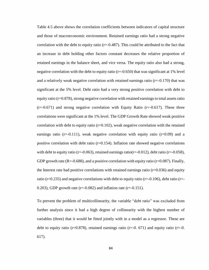
84
Table 4.5 above shows the correlation coefficients between indicators of capital structure
and those of macroeconomic environment. Retained earnings ratio had a strong negative
correlation with the debt to equity ratio (r=-0.487). This could be attributed to the fact that
an increase in debt holding other factors constant decreases the relative proportion of
retained earnings in the balance sheet, and vice versa. The equity ratio also had a strong,
negative correlation with the debt to equity ratio (r=-0.650) that was significant at 1% level
and a relatively weak negative correlation with retained earnings ratio (r=-0.170) that was
significant at the 5% level. Debt ratio had a very strong positive correlation with debt to
equity ratio (r=0.878), strong negative correlation with retained earnings to total assets ratio
(r=-0.671) and strong negative correlation with Equity Ratio (r=-0.617). These three
correlations were significant at the 1% level. The GDP Growth Rate showed weak positive
correlation with debt to equity ratio (r=0.102), weak negative correlation with the retained
earnings ratio (r=-0.111), weak negative correlation with equity ratio (r=0.09) and a
positive correlation with debt ratio (r=0.154). Inflation rate showed negative correlations
with debt to equity ratio (r=-0.063), retained earnings ratio(r=-0.012), debt ratio (r=-0.058),
GDP growth rate (R=-0.688), and a positive correlation with equity ratio (r=0.087). Finally,
the Interest rate had positive correlations with retained earnings ratio (r=0.036) and equity
ratio (r=0.235) and negative correlations with debt to equity ratio (r=-0.106), debt ratio (r=-
0.203), GDP growth rate (r=-0.082) and inflation rate (r=-0.151).
To prevent the problem of multicollinearity, the variable “debt ratio” was excluded from
further analysis since it had a high degree of collinearity with the highest number of
variables (three) that it would be fitted jointly with in a model as a regressor. These are
debt to equity ratio (r=0.878), retained earnings ratio (r=-0. 671) and equity ratio (r=-0.
617).
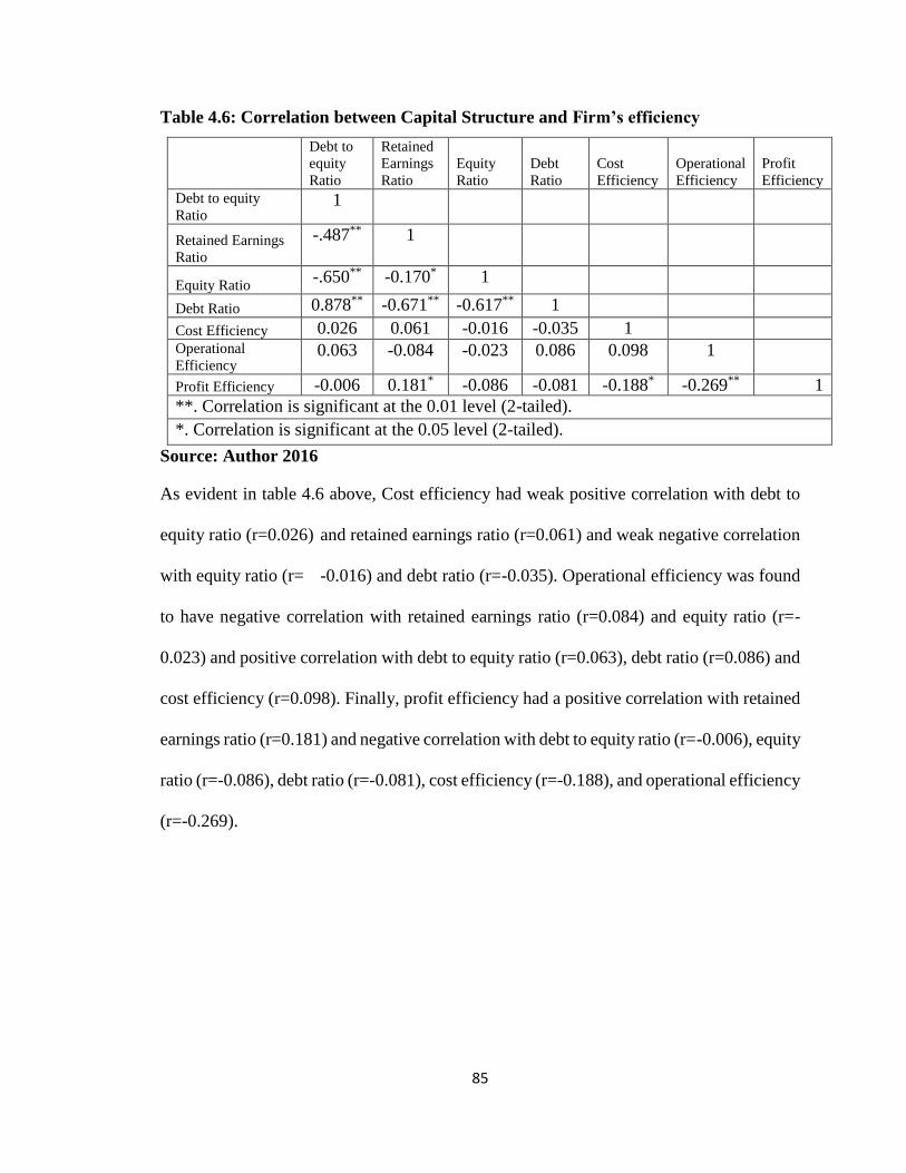
85
Table 4.6: Correlation between Capital Structure and Firm’s efficiency
Debt to
equity
Ratio
Retained
Earnings
Ratio
Equity
Ratio
Debt
Ratio
Cost
Efficiency
Operational
Efficiency
Profit
Efficiency
Debt to equity
Ratio 1
Retained Earnings
Ratio
-.487** 1
Equity Ratio -.650** -0.170* 1
Debt Ratio 0.878** -0.671** -0.617** 1
Cost Efficiency 0.026 0.061 -0.016 -0.035 1 Operational
Efficiency 0.063 -0.084 -0.023 0.086 0.098 1
Profit Efficiency -0.006 0.181* -0.086 -0.081 -0.188* -0.269** 1
**. Correlation is significant at the 0.01 level (2-tailed).
*. Correlation is significant at the 0.05 level (2-tailed).
Source: Author 2016
As evident in table 4.6 above, Cost efficiency had weak positive correlation with debt to
equity ratio (r=0.026) and retained earnings ratio (r=0.061) and weak negative correlation
with equity ratio (r= -0.016) and debt ratio (r=-0.035). Operational efficiency was found
to have negative correlation with retained earnings ratio (r=0.084) and equity ratio (r=-
0.023) and positive correlation with debt to equity ratio (r=0.063), debt ratio (r=0.086) and
cost efficiency (r=0.098). Finally, profit efficiency had a positive correlation with retained
earnings ratio (r=0.181) and negative correlation with debt to equity ratio (r=-0.006), equity
ratio (r=-0.086), debt ratio (r=-0.081), cost efficiency (r=-0.188), and operational efficiency
(r=-0.269).
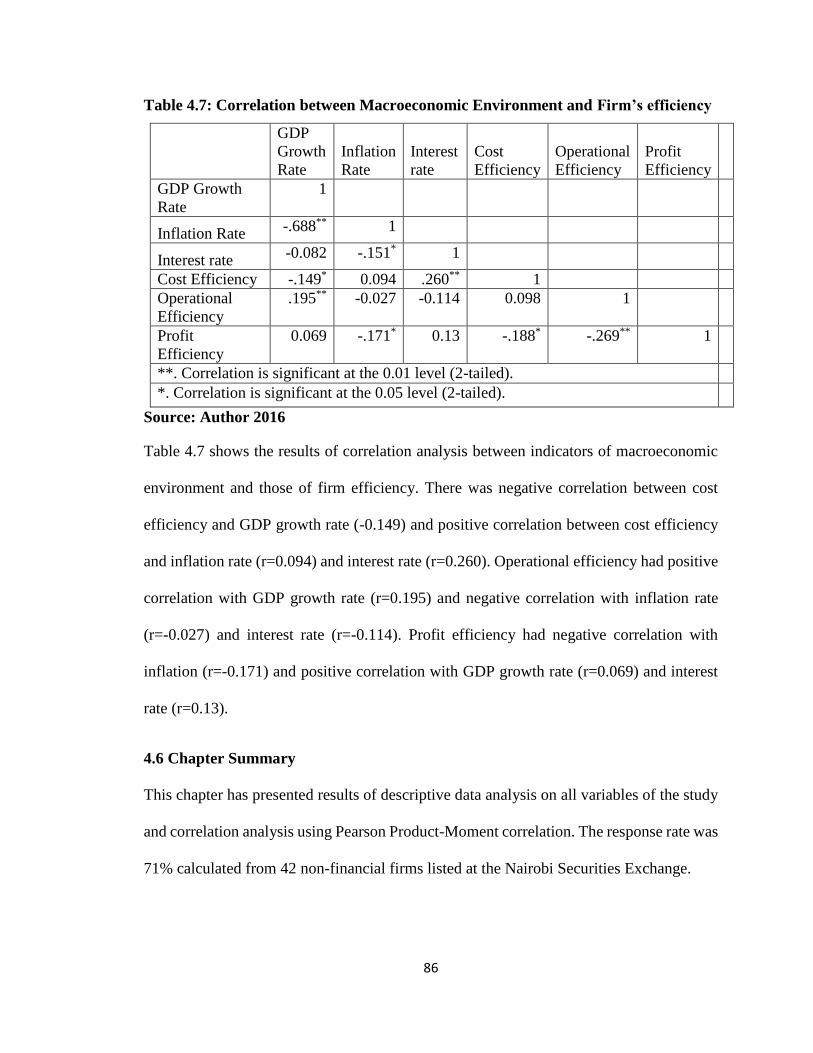
86
Table 4.7: Correlation between Macroeconomic Environment and Firm’s efficiency
GDP
Growth
Rate
Inflation
Rate
Interest
rate
Cost
Efficiency
Operational
Efficiency
Profit
Efficiency
GDP Growth
Rate
1
Inflation Rate -.688** 1
Interest rate -0.082 -.151* 1
Cost Efficiency -.149* 0.094 .260** 1
Operational
Efficiency
.195** -0.027 -0.114 0.098 1
Profit
Efficiency
0.069 -.171* 0.13 -.188* -.269** 1
**. Correlation is significant at the 0.01 level (2-tailed).
*. Correlation is significant at the 0.05 level (2-tailed).
Source: Author 2016
Table 4.7 shows the results of correlation analysis between indicators of macroeconomic
environment and those of firm efficiency. There was negative correlation between cost
efficiency and GDP growth rate (-0.149) and positive correlation between cost efficiency
and inflation rate (r=0.094) and interest rate (r=0.260). Operational efficiency had positive
correlation with GDP growth rate (r=0.195) and negative correlation with inflation rate
(r=-0.027) and interest rate (r=-0.114). Profit efficiency had negative correlation with
inflation (r=-0.171) and positive correlation with GDP growth rate (r=0.069) and interest
rate (r=0.13).
4.6 Chapter Summary
This chapter has presented results of descriptive data analysis on all variables of the study
and correlation analysis using Pearson Product-Moment correlation. The response rate was
71% calculated from 42 non-financial firms listed at the Nairobi Securities Exchange.
87
Descriptive statistics on capital structure (the independent variable) showed that the debt
to equity ratio variable had a mean of 0.478456, which essentially means that on average,
the firms had 48 cents in debt for every shilling of equity in their balance sheet. With a
standard deviation of 0.7, it is evident that debt to equity ratios of the sampled firms were
quite dispersed. This is affirmed further by the fact that the minimum value for debt to
equity was 0 (i.e. 100% equity financing) while the maximum value was 6.368421 (i.e
these firms were extremely leveraged during the pertinent period. They held Kshs 6.36 in
debt for each 1Kshs they had in equity). The debt to equity exhibited a very high level of
kurtosis (30.54732) and positive skewness (4.099016).
Retained earnings ratio showed that on average, 28.55% of the assets of the sampled firms
were financed using retained earnings. The least value for this statistic was -0.39362
(implying a loss making situation) while the highest value was 0.628952. Just like other
variables, the retained earnings ratio had a leptokurtic distribution (kurtosis=5.619681) but
in contrast with other variables, retained earnings ratio had a slightly negative skewness (-
0.9138) while equity ratio of the sampled firms was at a mean value of 0.526853. This
means that on average, the sampled firms had a tendency of financing just over half of their
assets using equity. This variable was quite stable (s.d. = 0.142063), with low dispersion
around the mean. The least value for this variable was 0.135714 while the highest was
1.058511, implying the rare situation of negative debt (-0.058511) that arises when a firm
has not only cleared its debts, but it has overpaid them. Technically, a negative liability is
a company asset, and so should be classified as a prepaid expense
The moderating variable macroeconomic environment is represented by the economic
growth rate, inflation rate, and interest rate. The mean for economic growth rate, inflation
88
rate, and interest rate are 4.12%, 11.59%, and 15.32% respectively. The results indicate
that the macroeconomic environment was favourable for business performance. While the
intervening variables comprising of cost, operational and profit efficiencies showed a mean
35.4%, 65.8% and 51.2%, respectively. The maximum cost efficiency, operational
efficiency, and profit efficiency were 72%, 89%, and 89% while the minimum cost
efficiency, operational efficiency, and profit efficiency were 10%, 14%, and 10%,
respectively.The mean for operational, cost and profit efficiency were 65%, 35% and 51%
respectively The results of the analysis demonstrate that the firms are using more inputs
for a unit of output compared to the best firm. Therefore, firms must sell their products at
higher prices to break even. This means that the outputs of the firms are not competitive in
the market leading to decline in revenues and profits. Consequently the dividends expected
to be paid to the owners will drop and this information will negatively affect the market
share price of the firm.
The market share prices (dependent variable) of the sampled firms showed that the share
prices were quite volatile across the panels, with a low of Kshs 1.75 and a high of Kshs
500. The mean of market share price was Kshs 71.44256. Additionally, the market share
price had a kurtosis of 7. 635904 and a skewness of 2.000684 implying that the market
share prices had fat tails, a leptokurtic distribution, and right skewness.
The results of correlation analysis shows that there was a relatively strong negative
correlation between debt to equity ratio and market share price. The correlation between
retained earnings ratio and market share price was strong (r=0.387) while the effect of
equity ratio on market share price was relatively weak and insignificant at both 5% and 1%
levels of significance. The strong, positive and significant correlation between retained
89
earnings and market share price can be attributed to many factors. Most important of all,
firms with high retention rates are viewed by the market as growth firms with huge
prospects for the future. Finally, Debt Ratio and market share price had a relatively strong
negative correlation (r = -.392). The negative effect of the debt to equity ratio and debt ratio
on the market share price shows a strong preference on unlevered stocks by investors. Due
to mandatory interest and principal repayments, highly indebted firms tend to have less
amounts of money that are available for distribution as dividends. Additionally, debt could
send a signal that the financial health of a firm is in turmoil, thereby making it less attractive
to investors.
To prevent the problem of multicollinearity, the variable “debt ratio” was excluded from
further analysis since it had a high degree of collinearity with the highest number of
variables (three) that it would not be fitted jointly in a model as a regressor. These are debt
to equity ratio (r=0.878), retained earnings ratio (r=-0. 671) and equity ratio (r=-0. 617).
90
CHAPTER FIVE
HYPOTHESES TESTING AND DISCUSSION OF FINDINGS
5.1 Introduction
In this chapter, the hypotheses of the study were tested and results of hypothesis testing
were discussed. For each of the four hypotheses, analysis started with the conducting of
diagnostic testing to appraise the conformance of the data with assumptions of Ordinary
Least Squares (OLS) panel regression analysis. This was to enable the researcher to use
robust models that are an exact fit for the data’s attributes thereby preventing the
probability of making either a type 1 error (rejecting a correct null hypothesis) or a type 2
error (failing to reject an incorrect null hypothesis).
5.1.1 Diagnostic Testing
Diagnostic tests are pre estimation procedures that evaluate whether the assumptions of
Ordinary Least Squares (OLS) panel regression analysis are upheld. In particular, a strong
linear relationship should not exist between any variables that are fitted jointly as regressors
in a model (no multicollinearity), there should be panel level stationarity, error terms
should be linearly independent (no autocorrelation), the variance of the error terms should
be constant (no heteroscedasticity), and the error terms should be normally distributed
(with a mean of zero and a constant variance). These assumptions and the particular tests
that were used to test for each of them are discussed in detail below.
5.1.1.1 Testing for Multicollinearity
The researcher used Variance inflation factors of the independent variables to test
multicollinearity. Variance inflation factors (VIF) measure how much the variance of the
estimated regression coefficients are inflated as compared to when the predictor variables
91
are not linearly related. As a rule of thumb, a variable whose VIF values are greater than
10 may merit further investigation. Tolerance, defined as 1/VIF, is used by many
researchers to check on the degree of collinearity. A tolerance value lower than 0.1 is
comparable to a VIF of 10. It means that the variable could be considered as a linear
combination of other independent variables.
5.1.1.2 Panel Level Stationarity
In order to analyze data using panel regression models, it should be stationary. Non
stationary data is likely to result in spurious regressions since mean and standard deviation
estimates derived from such data will be non-constant. To test the data for stationarity, the
Levin Lin Chu (LLC) Test unit root test was applied for all regression analysis of this study.
The null hypothesis of this test is that panels contain unit roots, whereas the alternative
hypothesis implies stationarity in the panel data. Pertaining rejection criteria, the null
hypothesis of a unit root is rejected if the p value of the LLC test is less than 5%.
5.1.1.3 Serial Correlation
Serial correlation (also called autocorrelation) is a phenomenon which occurs when the
error terms of regression variables for successive periods are correlated. When present in
a dataset, it can distort the efficiency of regression estimators. Using the Wooldridge test
for serial correlation; we tested this study’s data for the presence of autocorrelation. The
null hypothesis for this test is that there is no first order autocorrelation in the panels and
is rejected if the p value of the test is less than 5%.
92
5.1.1.4 Likelihood Ratio Test for Heteroscedasticity
Heteroscedasticity is a serious problem since it tends to inflate the standard errors, thereby
increasing the probability of committing a type two errors, i.e. failing to reject a false
hypothesis about a coefficient. The Likelihood Ratio test was used to test the data for
heteroscedasticity. The null hypothesis of the Likelihood Ratio test is that the data is
homoscedastic cross entities, i.e. the error terms have a constant variance. If the null is
rejected, the conclusion is that the data is heteroscedastic, i.e. the variance of error terms
across entities is not constant. The rejection criteria is that the null of homoscedasticity is
rejected if the p value of the Likelihood Ratio test is less than 5%.
5.1.2 Model Fitting
Classic panel data analysis suggests that the Hausman specification test should be used to
help the researcher in making a decision on whether to fit the random effects model or the
fixed effects model. These two models assume that the data meets all the assumptions of
regression analysis, i.e. no collinearity of regressors, no autocorrelation, and that the error
terms are normally distributed with a mean of 0 and a constant variance, i.e. no
heteroscedasticity.
Each violation of CLRM assumptions has a remedy. In instances where there is
multicollinearity, the variable with the highest Variance Inflation Factor (VIF) should be
excluded from further analysis. In cases of autocorrelation, a Prais Winsten Panel
Regression model should be fitted while in cases where there is heteroscedasticity, a
normal panel model (but with corrected/robust standard errors) should be fitted.
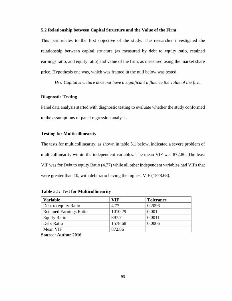
93
5.2 Relationship between Capital Structure and the Value of the Firm
This part relates to the first objective of the study. The researcher investigated the
relationship between capital structure (as measured by debt to equity ratio, retained
earnings ratio, and equity ratio) and value of the firm, as measured using the market share
price. Hypothesis one was, which was framed in the null below was tested.
H01: Capital structure does not have a significant influence the value of the firm.
Diagnostic Testing
Panel data analysis started with diagnostic testing to evaluate whether the study conformed
to the assumptions of panel regression analysis.
Testing for Multicollinearity
The tests for multicollinearity, as shown in table 5.1 below, indicated a severe problem of
multicollinearity within the independent variables. The mean VIF was 872.86. The least
VIF was for Debt to equity Ratio (4.77) while all other independent variables had VIFs that
were greater than 10, with debt ratio having the highest VIF (1578.68).
Table 5.1: Test for Multicollinearity
Variable VIF Tolerance
Debt to equity Ratio 4.77 0.2096
Retained Earnings Ratio 1010.29 0.001
Equity Ratio 897.7 0.0011
Debt Ratio 1578.68 0.0006
Mean VIF 872.86
Source: Author 2016
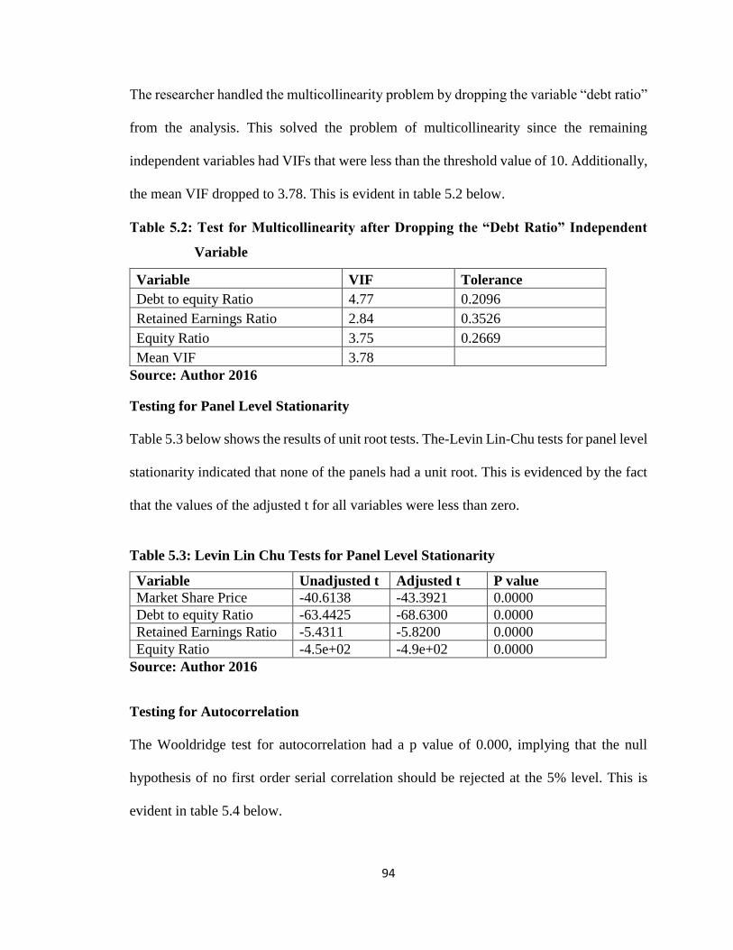
94
The researcher handled the multicollinearity problem by dropping the variable “debt ratio”
from the analysis. This solved the problem of multicollinearity since the remaining
independent variables had VIFs that were less than the threshold value of 10. Additionally,
the mean VIF dropped to 3.78. This is evident in table 5.2 below.
Table 5.2: Test for Multicollinearity after Dropping the “Debt Ratio” Independent
Variable
Variable VIF Tolerance
Debt to equity Ratio 4.77 0.2096
Retained Earnings Ratio 2.84 0.3526
Equity Ratio 3.75 0.2669
Mean VIF 3.78
Source: Author 2016
Testing for Panel Level Stationarity
Table 5.3 below shows the results of unit root tests. The-Levin Lin-Chu tests for panel level
stationarity indicated that none of the panels had a unit root. This is evidenced by the fact
that the values of the adjusted t for all variables were less than zero.
Table 5.3: Levin Lin Chu Tests for Panel Level Stationarity
Variable Unadjusted t Adjusted t P value
Market Share Price -40.6138 -43.3921 0.0000
Debt to equity Ratio -63.4425 -68.6300 0.0000
Retained Earnings Ratio -5.4311 -5.8200 0.0000
Equity Ratio -4.5e+02 -4.9e+02 0.0000
Source: Author 2016
Testing for Autocorrelation
The Wooldridge test for autocorrelation had a p value of 0.000, implying that the null
hypothesis of no first order serial correlation should be rejected at the 5% level. This is
evident in table 5.4 below.
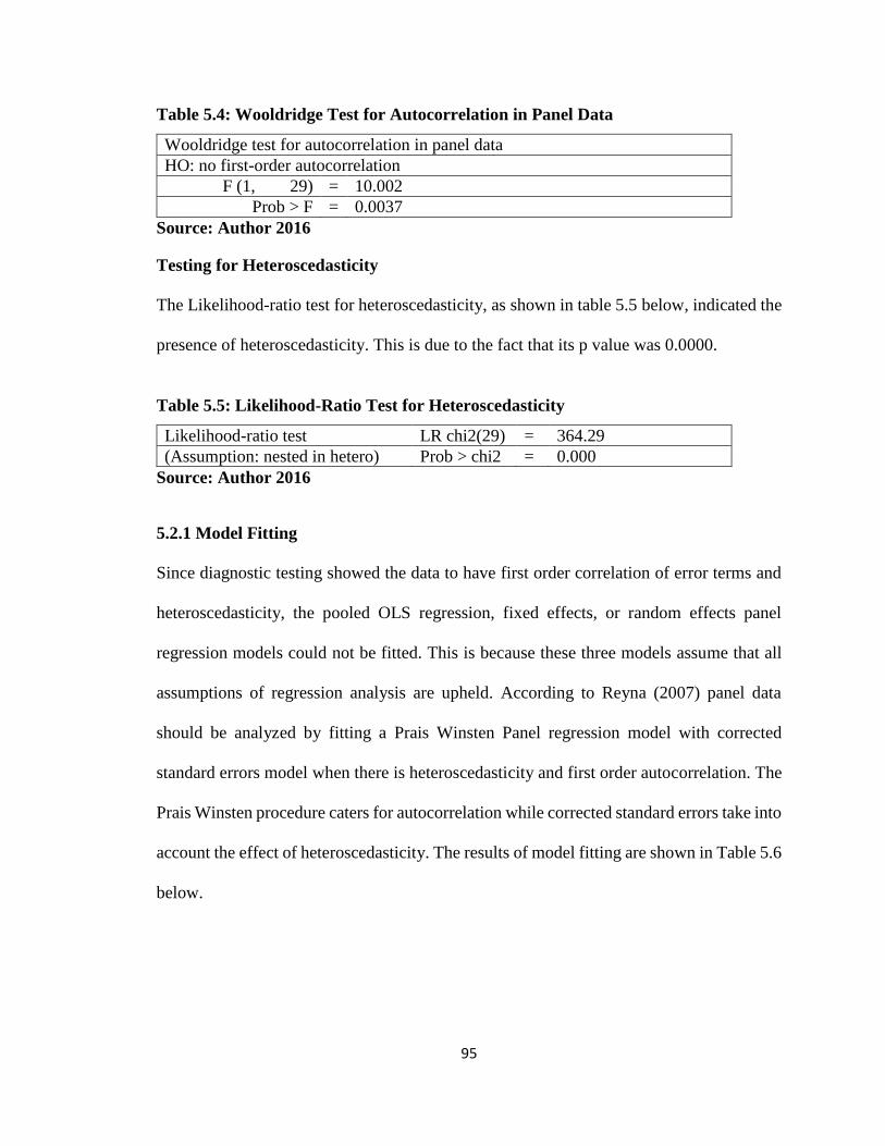
95
Table 5.4: Wooldridge Test for Autocorrelation in Panel Data
Wooldridge test for autocorrelation in panel data
HO: no first-order autocorrelation
F (1, 29) = 10.002
Prob > F = 0.0037
Source: Author 2016
Testing for Heteroscedasticity
The Likelihood-ratio test for heteroscedasticity, as shown in table 5.5 below, indicated the
presence of heteroscedasticity. This is due to the fact that its p value was 0.0000.
Table 5.5: Likelihood-Ratio Test for Heteroscedasticity
Likelihood-ratio test LR chi2(29) = 364.29
(Assumption: nested in hetero) Prob > chi2 = 0.000
Source: Author 2016
5.2.1 Model Fitting
Since diagnostic testing showed the data to have first order correlation of error terms and
heteroscedasticity, the pooled OLS regression, fixed effects, or random effects panel
regression models could not be fitted. This is because these three models assume that all
assumptions of regression analysis are upheld. According to Reyna (2007) panel data
should be analyzed by fitting a Prais Winsten Panel regression model with corrected
standard errors model when there is heteroscedasticity and first order autocorrelation. The
Prais Winsten procedure caters for autocorrelation while corrected standard errors take into
account the effect of heteroscedasticity. The results of model fitting are shown in Table 5.6
below.
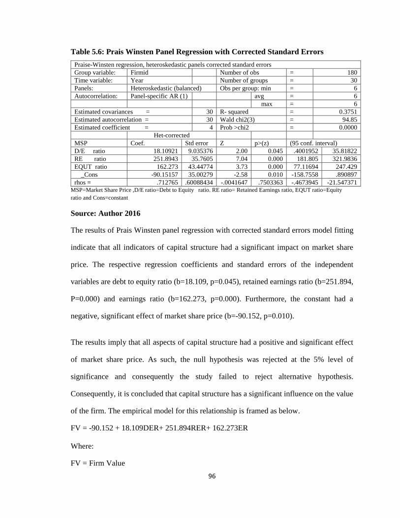
96
Table 5.6: Prais Winsten Panel Regression with Corrected Standard Errors
Praise-Winsten regression, heteroskedastic panels corrected standard errors
Group variable: Firmid Number of obs = 180
Time variable: Year Number of groups = 30
Panels: Heteroskedastic (balanced) Obs per group: min = 6
Autocorrelation: Panel-specific AR (1) avg = 6
max = 6
Estimated covariances = 30 R- squared = 0.3751
Estimated autocorrelation = 30 Wald chi2(3) = 94.85
Estimated coefficient = 4 Prob >chi2 = 0.0000
Het-corrected
MSP Coef. Std error Z p>(z) (95 conf. interval)
D/E ratio 18.10921 9.035376 2.00 0.045 .4001952 35.81822
RE ratio 251.8943 35.7605 7.04 0.000 181.805 321.9836
EQUT ratio 162.273 43.44774 3.73 0.000 77.11694 247.429
_Cons -90.15157 35.00279 -2.58 0.010 -158.7558 .890897
rhos = .712765 .60088434 -.0041647 .7503363 -.4673945 -21.547371 MSP=Market Share Price ,D/E ratio=Debt to Equity ratio. RE ratio= Retained Earnings ratio, EQUT ratio=Equity
ratio and Cons=constant
Source: Author 2016
The results of Prais Winsten panel regression with corrected standard errors model fitting
indicate that all indicators of capital structure had a significant impact on market share
price. The respective regression coefficients and standard errors of the independent
variables are debt to equity ratio (b=18.109, p=0.045), retained earnings ratio (b=251.894,
P=0.000) and earnings ratio (b=162.273, p=0.000). Furthermore, the constant had a
negative, significant effect of market share price (b=-90.152, p=0.010).
The results imply that all aspects of capital structure had a positive and significant effect
of market share price. As such, the null hypothesis was rejected at the 5% level of
significance and consequently the study failed to reject alternative hypothesis.
Consequently, it is concluded that capital structure has a significant influence on the value
of the firm. The empirical model for this relationship is framed as below.
FV = -90.152 + 18.109DER+ 251.894RER+ 162.273ER
Where:
FV = Firm Value
97
DER =Debt to Equity Ratio
RER= Retained Earnings Ratio
ER=Earnings Ratio
5.3 Moderating Effect of Macroeconomic Environment on the Relationship between
Capital Structure and the Value of the Firm
The second objective of the study was to investigate the moderating effect of the
Macroeconomic environment on the Relationship between Capital structure and the value
of the firm. The hypothesis that was tested in order to fulfil this objective was framed in
the null form as below:
H02: Macroeconomic environment does not significantly influence the relationship
between capital structure and firm value.
In testing the moderating effect of the macroeconomic environment on the relationship
between capital structure and the value of the firm was assessed using the method proposed
by Stone-Romero and Liakhovitski (2002). This involved testing the effects on the
dependent variable (firm value) of capital structure, moderator variable (macroeconomic
environment) and the respective interaction between capital structure and macroeconomic
environment. In the first step of this procedure, the independent variable (capital structure)
and moderating variable (macroeconomic environment) are jointly fitted in a panel
regression model as regressors of the dependent variable (firm value). In the second step
the independent variable, moderating variable, and a composite variable formed by
multiplying the dependent variable by the moderating variable (interaction variable) are
jointly regressed against the dependent variable. The moderating effect is deemed present
if the extent to which variability in the dependent variable can be attributed to variability
in the independent variables increases after inclusion of the interaction terms.
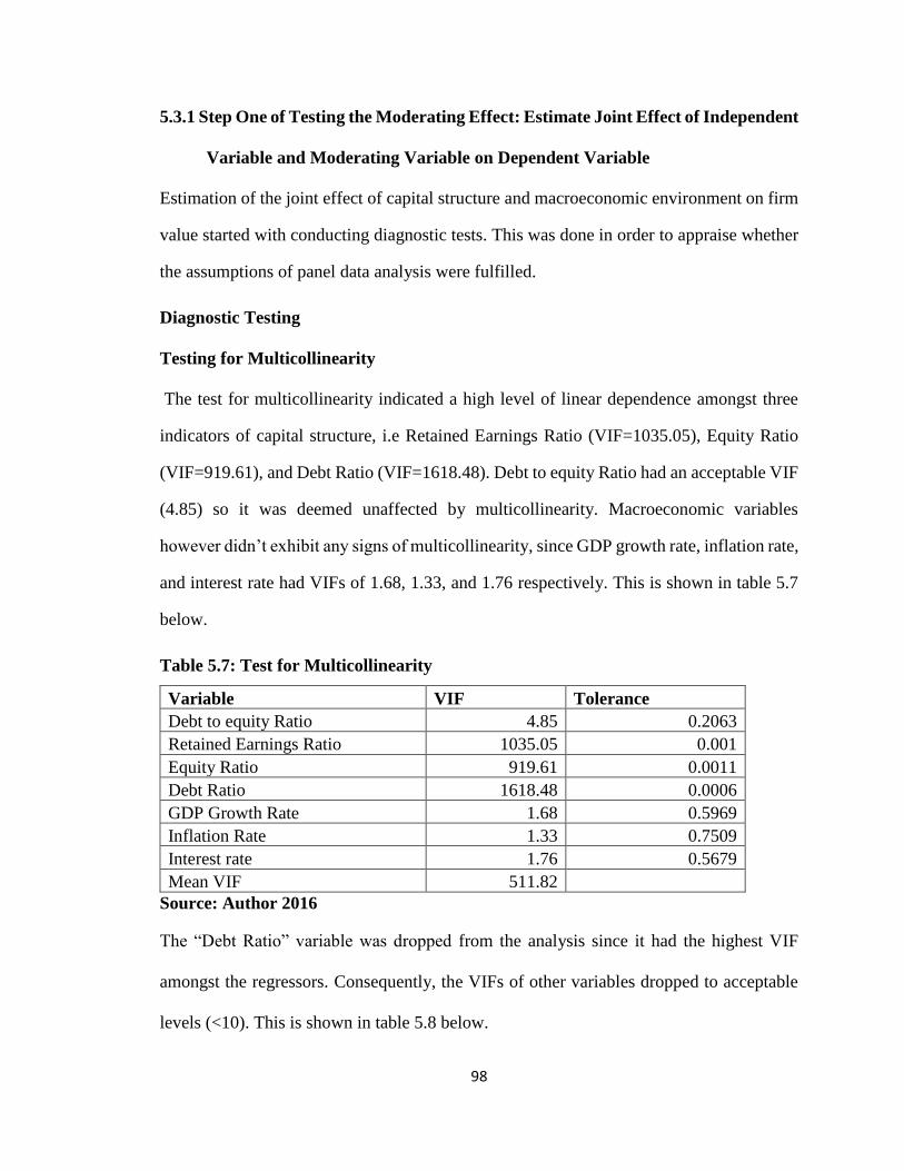
98
5.3.1 Step One of Testing the Moderating Effect: Estimate Joint Effect of Independent
Variable and Moderating Variable on Dependent Variable
Estimation of the joint effect of capital structure and macroeconomic environment on firm
value started with conducting diagnostic tests. This was done in order to appraise whether
the assumptions of panel data analysis were fulfilled.
Diagnostic Testing
Testing for Multicollinearity
The test for multicollinearity indicated a high level of linear dependence amongst three
indicators of capital structure, i.e Retained Earnings Ratio (VIF=1035.05), Equity Ratio
(VIF=919.61), and Debt Ratio (VIF=1618.48). Debt to equity Ratio had an acceptable VIF
(4.85) so it was deemed unaffected by multicollinearity. Macroeconomic variables
however didn’t exhibit any signs of multicollinearity, since GDP growth rate, inflation rate,
and interest rate had VIFs of 1.68, 1.33, and 1.76 respectively. This is shown in table 5.7
below.
Table 5.7: Test for Multicollinearity
Variable VIF Tolerance
Debt to equity Ratio 4.85 0.2063
Retained Earnings Ratio 1035.05 0.001
Equity Ratio 919.61 0.0011
Debt Ratio 1618.48 0.0006
GDP Growth Rate 1.68 0.5969
Inflation Rate 1.33 0.7509
Interest rate 1.76 0.5679
Mean VIF 511.82
Source: Author 2016
The “Debt Ratio” variable was dropped from the analysis since it had the highest VIF
amongst the regressors. Consequently, the VIFs of other variables dropped to acceptable
levels (<10). This is shown in table 5.8 below.
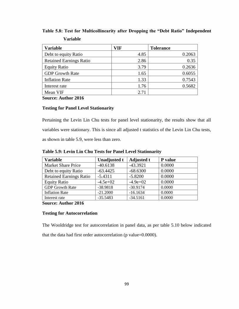
99
Table 5.8: Test for Multicollinearity after Dropping the “Debt Ratio” Independent
Variable
Variable VIF Tolerance
Debt to equity Ratio 4.85 0.2063
Retained Earnings Ratio 2.86 0.35
Equity Ratio 3.79 0.2636
GDP Growth Rate 1.65 0.6055
Inflation Rate 1.33 0.7543
Interest rate 1.76 0.5682
Mean VIF 2.71
Source: Author 2016
Testing for Panel Level Stationarity
Pertaining the Levin Lin Chu tests for panel level stationarity, the results show that all
variables were stationary. This is since all adjusted t statistics of the Levin Lin Chu tests,
as shown in table 5.9, were less than zero.
Table 5.9: Levin Lin Chu Tests for Panel Level Stationarity
Variable Unadjusted t Adjusted t P value
Market Share Price -40.6138 -43.3921 0.0000
Debt to equity Ratio -63.4425 -68.6300 0.0000
Retained Earnings Ratio -5.4311 -5.8200 0.0000
Equity Ratio -4.5e+02 -4.9e+02 0.0000 GDP Growth Rate -38.9818 -30.9174 0.0000
Inflation Rate -21.2000 -16.1634 0.0000
Interest rate -35.5483 -34.5161 0.0000
Source: Author 2016
Testing for Autocorrelation
The Wooldridge test for autocorrelation in panel data, as per table 5.10 below indicated
that the data had first order autocorrelation (p value=0.0000).
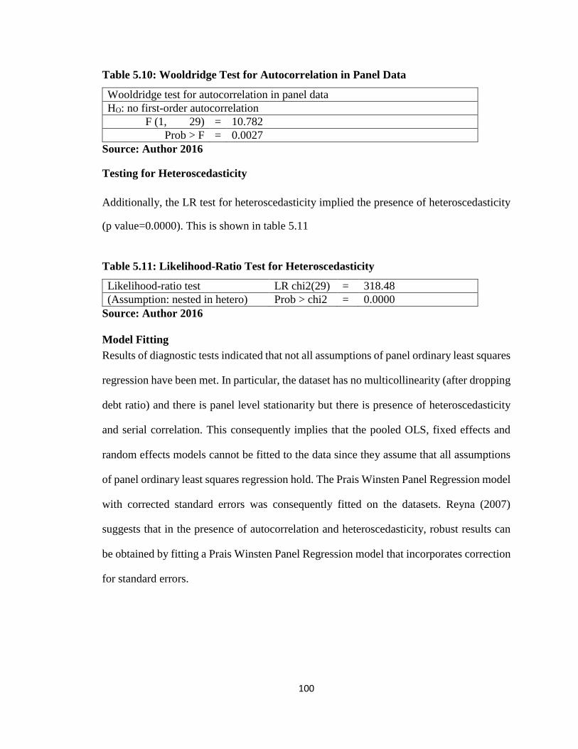
100
Table 5.10: Wooldridge Test for Autocorrelation in Panel Data
Wooldridge test for autocorrelation in panel data
HO: no first-order autocorrelation
F (1, 29) = 10.782
Prob > F = 0.0027
Source: Author 2016
Testing for Heteroscedasticity
Additionally, the LR test for heteroscedasticity implied the presence of heteroscedasticity
(p value=0.0000). This is shown in table 5.11
Table 5.11: Likelihood-Ratio Test for Heteroscedasticity
Likelihood-ratio test LR chi2(29) = 318.48
(Assumption: nested in hetero) Prob > chi2 = 0.0000
Source: Author 2016
Model Fitting
Results of diagnostic tests indicated that not all assumptions of panel ordinary least squares
regression have been met. In particular, the dataset has no multicollinearity (after dropping
debt ratio) and there is panel level stationarity but there is presence of heteroscedasticity
and serial correlation. This consequently implies that the pooled OLS, fixed effects and
random effects models cannot be fitted to the data since they assume that all assumptions
of panel ordinary least squares regression hold. The Prais Winsten Panel Regression model
with corrected standard errors was consequently fitted on the datasets. Reyna (2007)
suggests that in the presence of autocorrelation and heteroscedasticity, robust results can
be obtained by fitting a Prais Winsten Panel Regression model that incorporates correction
for standard errors.
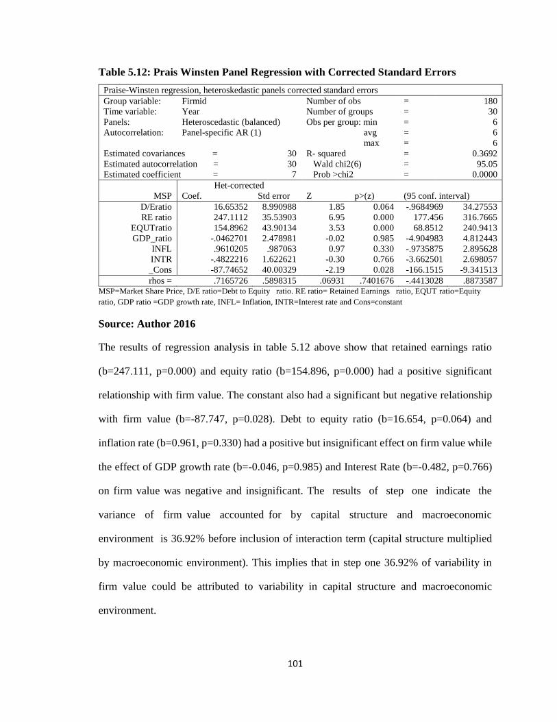
101
Table 5.12: Prais Winsten Panel Regression with Corrected Standard Errors
Praise-Winsten regression, heteroskedastic panels corrected standard errors
Group variable: Firmid Number of obs = 180
Time variable: Year Number of groups = 30
Panels: Heteroscedastic (balanced) Obs per group: min = 6
Autocorrelation: Panel-specific AR (1) avg = 6
max = 6
Estimated covariances = 30 R- squared = 0.3692
Estimated autocorrelation = 30 Wald chi2(6) = 95.05
Estimated coefficient = 7 Prob >chi2 = 0.0000
Het-corrected
MSP Coef. Std error Z p>(z) (95 conf. interval)
D/Eratio 16.65352 8.990988 1.85 0.064 -.9684969 34.27553
RE ratio 247.1112 35.53903 6.95 0.000 177.456 316.7665
EQUTratio 154.8962 43.90134 3.53 0.000 68.8512 240.9413
GDP_ratio -.0462701 2.478981 -0.02 0.985 -4.904983 4.812443
INFL .9610205 .987063 0.97 0.330 -.9735875 2.895628
INTR -.4822216 1.622621 -0.30 0.766 -3.662501 2.698057
_Cons -87.74652 40.00329 -2.19 0.028 -166.1515 -9.341513
rhos = .7165726 .5898315 .06931 .7401676 -.4413028 .8873587 MSP=Market Share Price, D/E ratio=Debt to Equity ratio. RE ratio= Retained Earnings ratio, EQUT ratio=Equity
ratio, GDP ratio =GDP growth rate, INFL= Inflation, INTR=Interest rate and Cons=constant
Source: Author 2016
The results of regression analysis in table 5.12 above show that retained earnings ratio
(b=247.111, p=0.000) and equity ratio (b=154.896, p=0.000) had a positive significant
relationship with firm value. The constant also had a significant but negative relationship
with firm value (b=-87.747, p=0.028). Debt to equity ratio (b=16.654, p=0.064) and
inflation rate (b=0.961, p=0.330) had a positive but insignificant effect on firm value while
the effect of GDP growth rate (b=-0.046, p=0.985) and Interest Rate (b=-0.482, p=0.766)
on firm value was negative and insignificant. The results of step one indicate the
variance of firm value accounted for by capital structure and macroeconomic
environment is 36.92% before inclusion of interaction term (capital structure multiplied
by macroeconomic environment). This implies that in step one 36.92% of variability in
firm value could be attributed to variability in capital structure and macroeconomic
environment.
102
The empirical model for this relationship can therefore be framed as:
FV = -87.747 +16.654DER+ 247.111RER+ 154.896ER - 0.046GGR + INFR0.961 -
INTR0.482
Where:
FV = Firm Value
DER =Debt to Equity Ratio
RER= Retained Earnings Ratio
ER=Earnings Ratio
GGR = GDP Growth Rate
INFR= Inflation Rate
INTR= Interest Rate
The model above can be further simplified by dropping the insignificant variables from it.
In essence, if the p value is greater than 5%, the effect of the pertinent regressor on the
dependent variable is not different from that of zero. Four variables, i.e. debt to equity ratio,
GDP growth rate, inflation rate, and interest rate were not significant. The model can
therefore be rewritten as below:
FV = -87.747 + 247.111RER+ 154.896ER
5.3.2 Step Two of Testing the Moderating Effect: Estimate Joint Effect of
Independent Variable, Moderating Variable and Interaction Terms on
Dependent Variable
The second step of testing hypothesis two entailed estimating the joint effect of the
independent variable (capital structure), moderating variable (macroeconomic
environment), and interaction terms (capital structure*macroeconomic environment) on
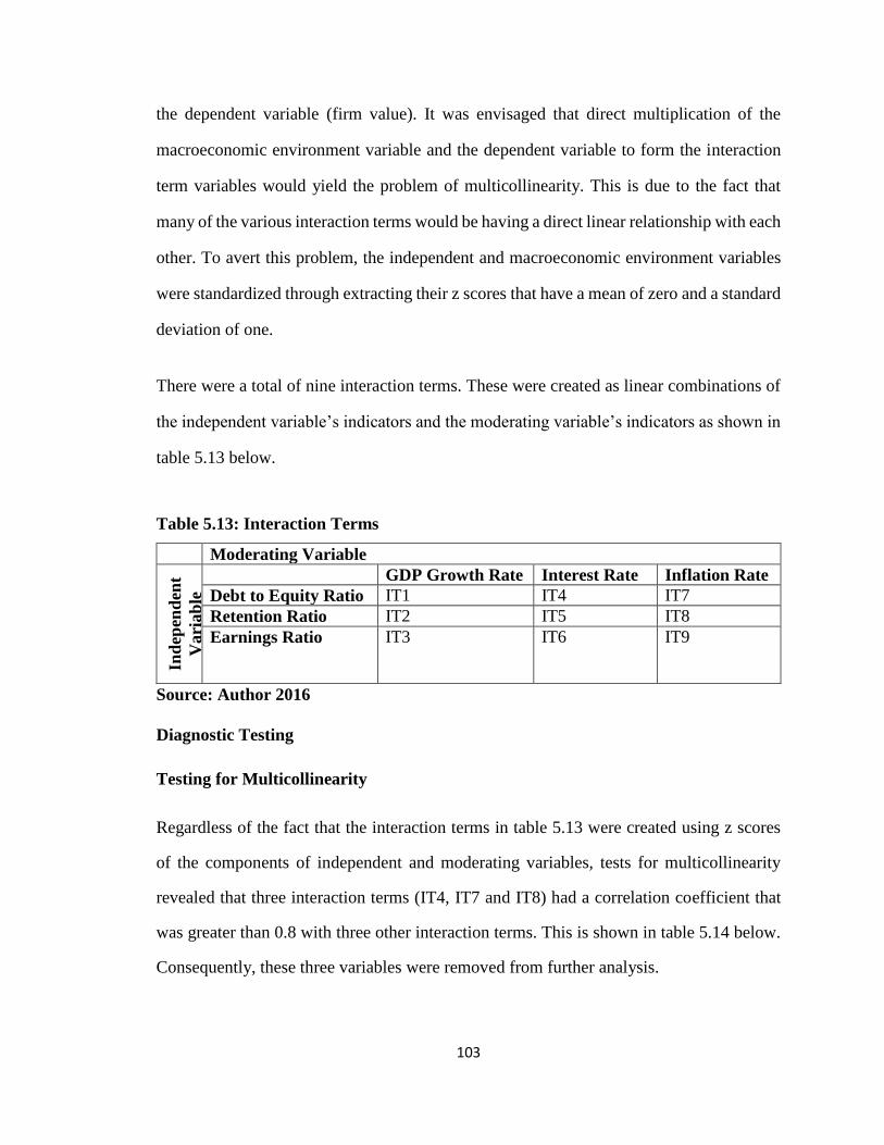
103
the dependent variable (firm value). It was envisaged that direct multiplication of the
macroeconomic environment variable and the dependent variable to form the interaction
term variables would yield the problem of multicollinearity. This is due to the fact that
many of the various interaction terms would be having a direct linear relationship with each
other. To avert this problem, the independent and macroeconomic environment variables
were standardized through extracting their z scores that have a mean of zero and a standard
deviation of one.
There were a total of nine interaction terms. These were created as linear combinations of
the independent variable’s indicators and the moderating variable’s indicators as shown in
table 5.13 below.
Table 5.13: Interaction Terms
Moderating Variable
Ind
epen
den
t
Vari
ab
le
GDP Growth Rate Interest Rate Inflation Rate
Debt to Equity Ratio IT1 IT4 IT7
Retention Ratio IT2 IT5 IT8
Earnings Ratio IT3 IT6 IT9
Source: Author 2016
Diagnostic Testing
Testing for Multicollinearity
Regardless of the fact that the interaction terms in table 5.13 were created using z scores
of the components of independent and moderating variables, tests for multicollinearity
revealed that three interaction terms (IT4, IT7 and IT8) had a correlation coefficient that
was greater than 0.8 with three other interaction terms. This is shown in table 5.14 below.
Consequently, these three variables were removed from further analysis.
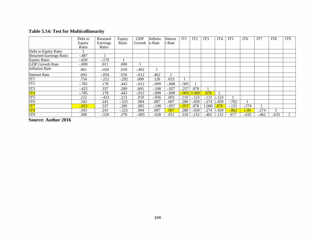
104
Table 5.14: Test for Multicollinearity
Debt to Equity Ratio
Retained Earnings
Ratio
Equity Ratio
GDP Growth
Inflation Rate
Interest Rate
IT1 IT2 IT3 IT4 IT5 IT6 IT7 IT8 IT9
Debt to Equity Ratio 1 Retained Earnings Ratio -.487 1 Equity Ratio -.650 -.170 1 GDP Growth Rate -.009 .011 .000 1 Inflation Rate .061 -.026 .010 -.402 1
Interest Rate .043 -.054 .016 -.612 .462 1 IT1 .754 -.212 -.292 .008 .126 .023 1 IT2 -.785 .178 .443 -.012 -.099 -.008 -.305 1
IT3 -.425 .337 .289 .005 -.108 -.057 -.257 .878 1 IT4 -.785 .178 .443 -.012 -.099 -.008 -.905 1.000 .878 1 IT5 .122 -.423 .213 .010 -.056 .003 .119 -.123 -.131 -.123 1 IT6 .343 .241 -.525 .004 .087 .007 .288 -.459 -.274 -.459 -.762 1 IT7 -.825 .337 .289 .005 -.108 -.057 -.957 .878 1.000 .878 -.131 -.274 1 IT8 .343 .241 -.525 .004 .087 .907 .288 -.459 -.274 -.459 -.862 1.00 -.274 1 IT9 .308 -.550 .278 -.005 -.028 .051 .318 -.152 -.462 -.152 .677 -.635 -.462 -.635 1
Source: Author 2016
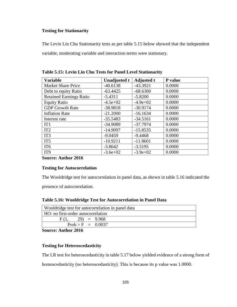
105
Testing for Stationarity
The Levin Lin Chu Stationarity tests as per table 5.15 below showed that the independent
variable, moderating variable and interaction terms were stationary.
Table 5.15: Levin Lin Chu Tests for Panel Level Stationarity
Variable Unadjusted t Adjusted t P value
Market Share Price -40.6138 -43.3921 0.0000
Debt to equity Ratio -63.4425 -68.6300 0.0000
Retained Earnings Ratio -5.4311 -5.8200 0.0000
Equity Ratio -4.5e+02 -4.9e+02 0.0000
GDP Growth Rate -38.9818 -30.9174 0.0000
Inflation Rate -21.2000 -16.1634 0.0000
Interest rate -35.5483 -34.5161 0.0000
IT1 -34.9089 -37.7974 0.0000
IT2 -14.9097 -15.8535 0.0000
IT3 -9.0459 -9.4468 0.0000
IT5 -10.9211 -11.8601 0.0000
IT6 -3.8642 -3.5195 0.0000
IT9 -3.6e+02 -3.9e+02 0.0000
Source: Author 2016
Testing for Autocorrelation
The Wooldridge test for autocorrelation in panel data, as shown in table 5.16 indicated the
presence of autocorrelation.
Table 5.16: Wooldridge Test for Autocorrelation in Panel Data
Wooldridge test for autocorrelation in panel data
HO: no first-order autocorrelation
F (1, 29) = 9.968
Prob > F = 0.0037
Source: Author 2016
Testing for Heteroscedasticity
The LR test for heteroscedasticity in table 5.17 below yielded evidence of a strong form of
homoscedasticity (no heteroscedasticity). This is because its p value was 1.0000.
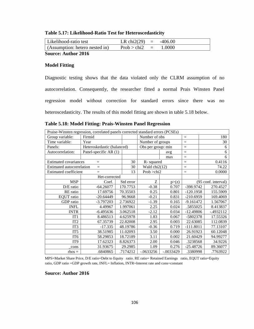
106
Table 5.17: Likelihood-Ratio Test for Heteroscedasticity
Likelihood-ratio test LR chi2(29) = -406.00
(Assumption: hetero nested in) Prob > chi2 = 1.0000
Source: Author 2016
Model Fitting
Diagnostic testing shows that the data violated only the CLRM assumption of no
autocorrelation. Consequently, the researcher fitted a normal Prais Winsten Panel
regression model without correction for standard errors since there was no
heteroscedasticity. The results of this model fitting are shown in table 5.18 below.
Table 5.18: Model Fitting: Prais-Winsten Panel Regression
Praise-Winsten regression, correlated panels corrected standard errors (PCSEs)
Group variable: Firmid Number of obs = 180
Time variable: Year Number of groups = 30
Panels: Heteroskedastic (balanced) Obs per group: min = 6
Autocorrelation: Panel-specific AR (1) avg = 6
max = 6
Estimated covariances = 30 R- squared = 0.4116
Estimated autocorrelation = 30 Wald chi2(12) = 74.22
Estimated coefficient = 13 Prob >chi2 = 0.0000
Het-corrected
MSP Coef. Std error Z p>(z) (95 conf. interval)
D/E ratio -64.26077 170.7753 -0.38 0.707 -398.9742 270.4527
RE ratio 17.69756 70.35503 0.25 0.801 -120.1958 155.5909
EQUT ratio -20.64449 96.9668 -0.21 0.831 -210.6959 169.4069
GDP ratio -3.797203 2.736922 -1.39 0.165 -9.161472 1.567067
INFL 4.49967 1.997061 2.25 0.024 .5855025 8.413837
INTR -6.495636 3.062518 -2.12 0.034 -12.49806 -.4932112
IT1 8.486513 4.625978 1.83 0.067 -5802378 17.55326
IT2 67.35739 22.82008 2.95 0.003 22.63085 112.0839
IT3 -17.335 48.19786 -0.36 0.719 -111.8011 77.13107
IT5 38.51985 11.02093 3.50 0.000 26.91923 60.12048
IT6 58.29853 18.72189 3.11 0.002 21.60429 94.99277
IT9 17.62323 8.826373 2.00 0.046 .3238568 34.9226
_cons 31.93675 29.2985 1.09 0.276 -25.48726 89.36077
rhos = .6840865 .7174212 -.0633256 -.0033429 .3380998 .7763922
MPS=Market Share Price, D/E ratio=Debt to Equity ratio. RE ratio= Retained Earnings ratio, EQUT ratio=Equity
ratio, GDP ratio =GDP growth rate, INFL= Inflation, INTR=Interest rate and cons=constant
Source: Author 2016
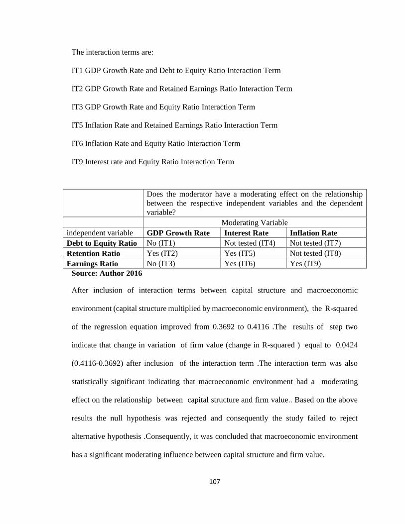
107
The interaction terms are:
IT1 GDP Growth Rate and Debt to Equity Ratio Interaction Term
IT2 GDP Growth Rate and Retained Earnings Ratio Interaction Term
IT3 GDP Growth Rate and Equity Ratio Interaction Term
IT5 Inflation Rate and Retained Earnings Ratio Interaction Term
IT6 Inflation Rate and Equity Ratio Interaction Term
IT9 Interest rate and Equity Ratio Interaction Term
Does the moderator have a moderating effect on the relationship
between the respective independent variables and the dependent
variable?
Moderating Variable
independent variable GDP Growth Rate Interest Rate Inflation Rate
Debt to Equity Ratio No (IT1) Not tested (IT4) Not tested (IT7)
Retention Ratio Yes (IT2) Yes (IT5) Not tested (IT8)
Earnings Ratio No (IT3) Yes (IT6) Yes (IT9)
Source: Author 2016
After inclusion of interaction terms between capital structure and macroeconomic
environment (capital structure multiplied by macroeconomic environment), the R-squared
of the regression equation improved from 0.3692 to 0.4116 .The results of step two
indicate that change in variation of firm value (change in R-squared ) equal to 0.0424
(0.4116-0.3692) after inclusion of the interaction term .The interaction term was also
statistically significant indicating that macroeconomic environment had a moderating
effect on the relationship between capital structure and firm value.. Based on the above
results the null hypothesis was rejected and consequently the study failed to reject
alternative hypothesis .Consequently, it was concluded that macroeconomic environment
has a significant moderating influence between capital structure and firm value.
108
5.4 Intervening Effect of Firm efficiency on the Relationship between Capital
Structure and the Value of the Firm
This part relates to the third objective of the study. The researcher tested the intervening
effect of firm efficiency (as measured by cost efficiency, operational efficiency, and profit
efficiency). Hypothesis three was framed in the null below:
H03: Firm’s efficiency do not have a significant influence on the value of the firm.
Four steps were followed to test the Intervening effect in line with the process advocated
by Baron and Kenny (1986). In step one of testing this effect, regression analysis was
performed to assess the relationship between (dependent variable) and (independent
variable) while ignoring the mediator. In step two, panel regression was carried out
between the independent variables (capital structure) and the intervening variables (firm
efficiency) while ignoring the dependent variable (firm value). In the third step of the
mediation analysis, regression analysis was performed to assess the relationship between
firm efficiency (intervening variable) and firm value (dependent variable) while ignoring
the independent variable (capital structure). The fourth step of the mediation analysis was
performed to assess the joint effect of firm’s efficiency (intervening variable) and capital
structure (independent variable) on firm value (dependent variable). Intervention is deemed
to occur if capital structure predicts firm value; capital structure predicts firm efficiency
and firm efficiency predict firm value. An additional requirement to validate the presence
of the intervening effect is that capital structure should predict firm value in a model in
which firm efficiency are included jointly with capital structure as regressors.
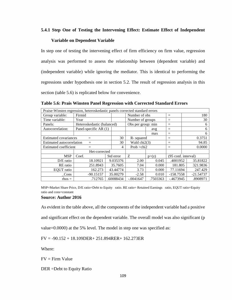
109
5.4.1 Step One of Testing the Intervening Effect: Estimate Effect of Independent
Variable on Dependent Variable
In step one of testing the intervening effect of firm efficiency on firm value, regression
analysis was performed to assess the relationship between (dependent variable) and
(independent variable) while ignoring the mediator. This is identical to performing the
regressions under hypothesis one in section 5.2. The result of regression analysis in this
section (table 5.6) is replicated below for convenience.
Table 5.6: Prais Winsten Panel Regression with Corrected Standard Errors
Praise-Winsten regression, heteroskedastic panels corrected standard errors
Group variable: Firmid Number of obs = 180
Time variable: Year Number of groups = 30
Panels: Heteroskedastic (balanced) Obs per group: min = 6
Autocorrelation: Panel-specific AR (1) avg = 6
max = 6
Estimated covariances = 30 R- squared = 0.3751
Estimated autocorrelation = 30 Wald chi2(3) = 94.85
Estimated coefficient = 4 Prob >chi2 = 0.0000
Het-corrected
MSP Coef. Std error Z p>(z) (95 conf. interval)
D/E ratio 18.10921 9.035376 2.00 0.045 .4001952 35.81822
RE ratio 251.8943 35.7605 7.04 0.000 181.805 321.9836
EQUT ratio 162.273 43.44774 3.73 0.000 77.11694 247.429
_Cons -90.15157 35.00279 -2.58 0.010 -158.7558 -21.54737
rhos = .712765 .60088434 -.0041647 .7503363 -.4673945 .8908971
MSP=Market Share Price, D/E ratio=Debt to Equity ratio. RE ratio= Retained Earnings ratio, EQUT ratio=Equity
ratio and cons=constant
Source: Author 2016
As evident in the table above, all the components of the independent variable had a positive
and significant effect on the dependent variable. The overall model was also significant (p
value=0.0000) at the 5% level. The model in step one was specified as:
FV = -90.152 + 18.109DER+ 251.894RER+ 162.273ER
Where:
FV = Firm Value
DER =Debt to Equity Ratio
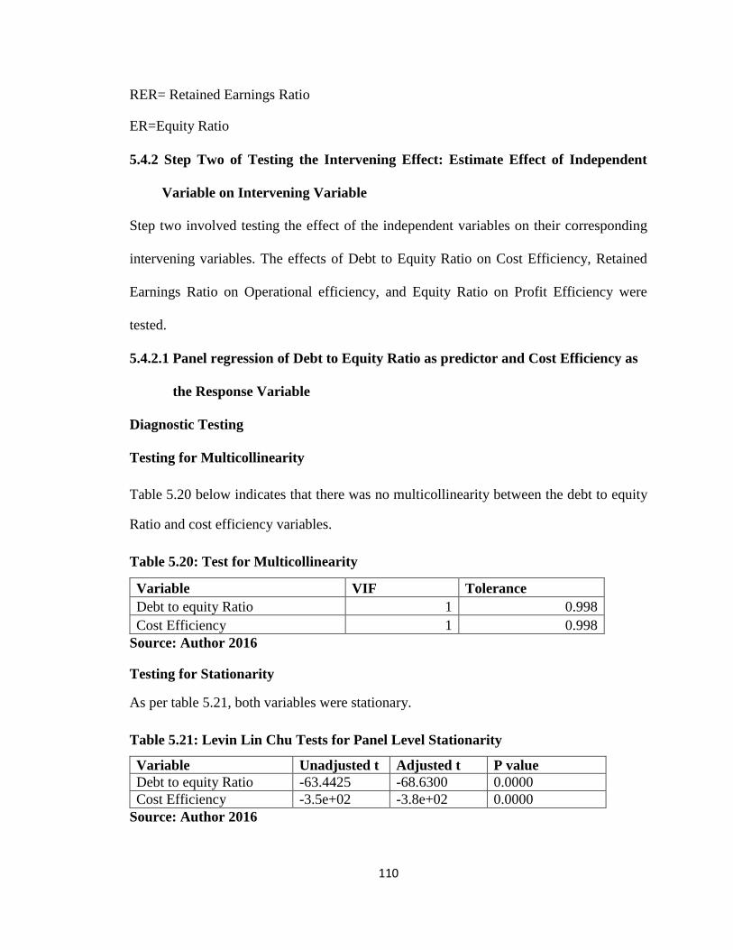
110
RER= Retained Earnings Ratio
ER=Equity Ratio
5.4.2 Step Two of Testing the Intervening Effect: Estimate Effect of Independent
Variable on Intervening Variable
Step two involved testing the effect of the independent variables on their corresponding
intervening variables. The effects of Debt to Equity Ratio on Cost Efficiency, Retained
Earnings Ratio on Operational efficiency, and Equity Ratio on Profit Efficiency were
tested.
5.4.2.1 Panel regression of Debt to Equity Ratio as predictor and Cost Efficiency as
the Response Variable
Diagnostic Testing
Testing for Multicollinearity
Table 5.20 below indicates that there was no multicollinearity between the debt to equity
Ratio and cost efficiency variables.
Table 5.20: Test for Multicollinearity
Variable VIF Tolerance
Debt to equity Ratio 1 0.998
Cost Efficiency 1 0.998
Source: Author 2016
Testing for Stationarity
As per table 5.21, both variables were stationary.
Table 5.21: Levin Lin Chu Tests for Panel Level Stationarity
Variable Unadjusted t Adjusted t P value
Debt to equity Ratio -63.4425 -68.6300 0.0000
Cost Efficiency -3.5e+02 -3.8e+02 0.0000
Source: Author 2016
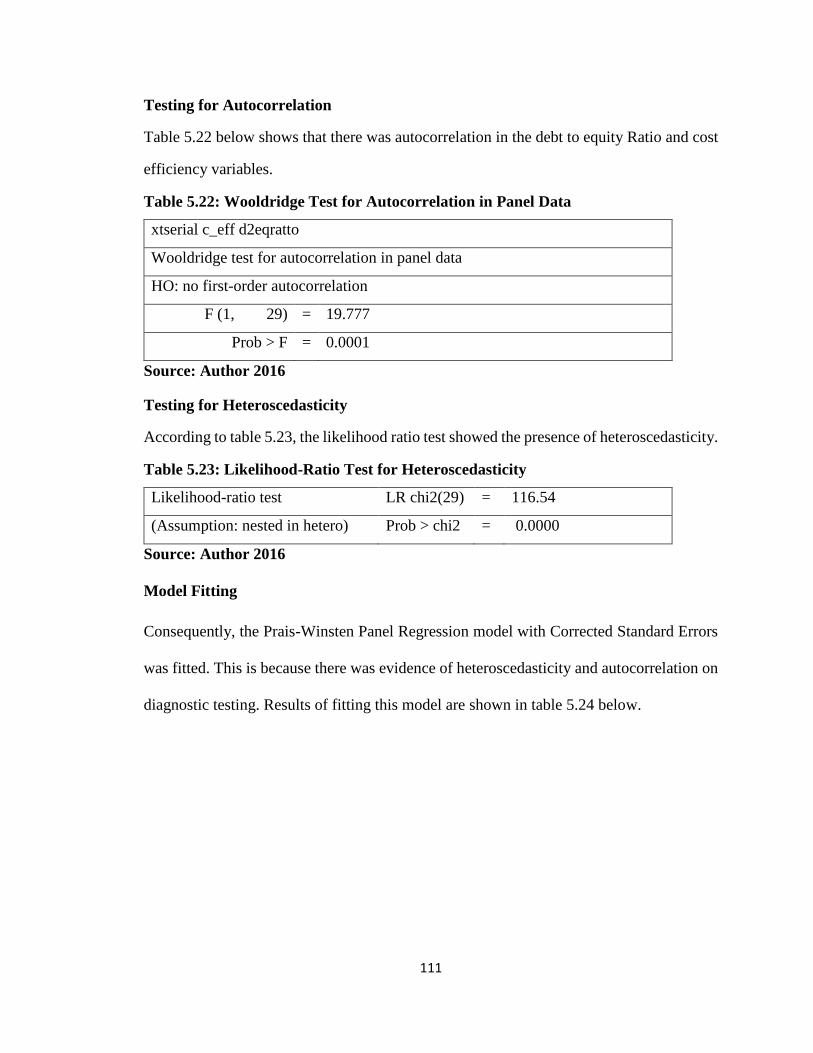
111
Testing for Autocorrelation
Table 5.22 below shows that there was autocorrelation in the debt to equity Ratio and cost
efficiency variables.
Table 5.22: Wooldridge Test for Autocorrelation in Panel Data
xtserial c_eff d2eqratto
Wooldridge test for autocorrelation in panel data
HO: no first-order autocorrelation
F (1, 29) = 19.777
Prob > F = 0.0001
Source: Author 2016
Testing for Heteroscedasticity
According to table 5.23, the likelihood ratio test showed the presence of heteroscedasticity.
Table 5.23: Likelihood-Ratio Test for Heteroscedasticity
Likelihood-ratio test LR chi2(29) = 116.54
(Assumption: nested in hetero) Prob > chi2 = 0.0000
Source: Author 2016
Model Fitting
Consequently, the Prais-Winsten Panel Regression model with Corrected Standard Errors
was fitted. This is because there was evidence of heteroscedasticity and autocorrelation on
diagnostic testing. Results of fitting this model are shown in table 5.24 below.
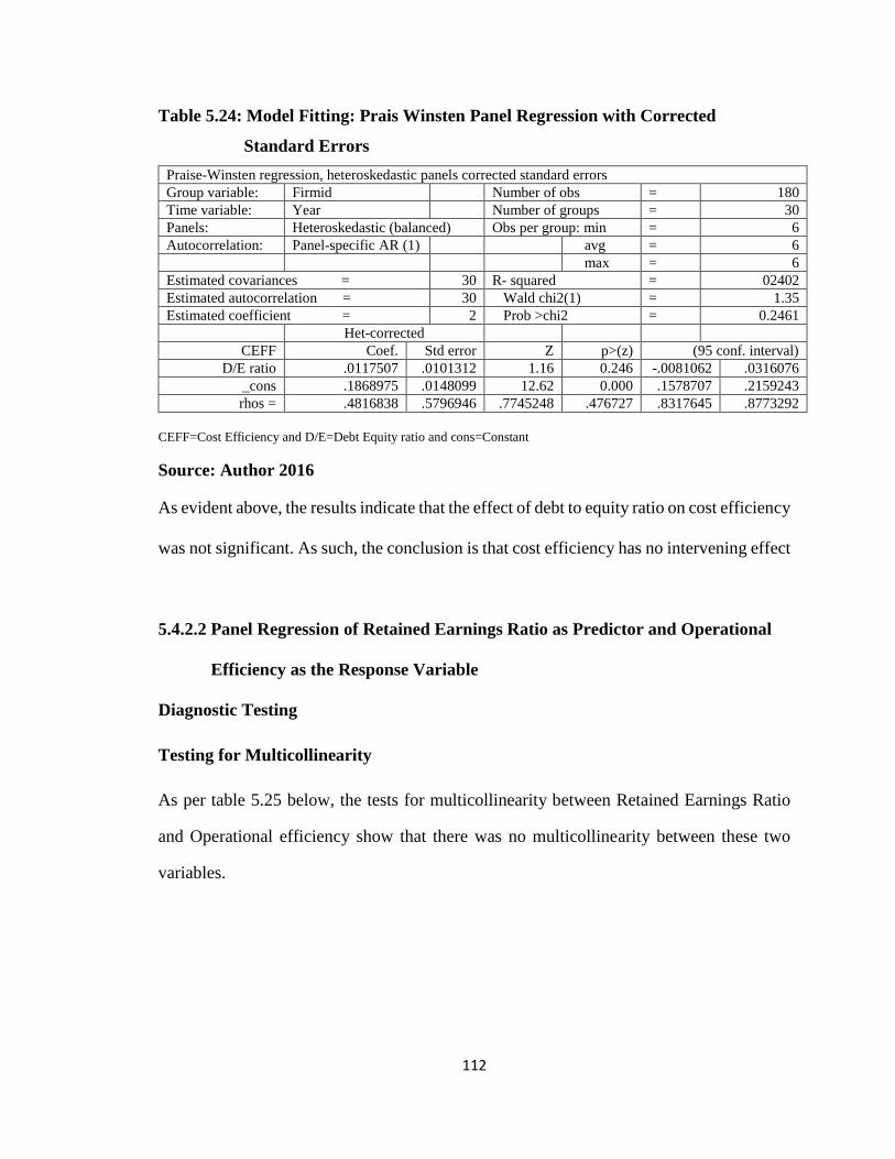
112
Table 5.24: Model Fitting: Prais Winsten Panel Regression with Corrected
Standard Errors
Praise-Winsten regression, heteroskedastic panels corrected standard errors
Group variable: Firmid Number of obs = 180
Time variable: Year Number of groups = 30
Panels: Heteroskedastic (balanced) Obs per group: min = 6
Autocorrelation: Panel-specific AR (1) avg = 6
max = 6
Estimated covariances = 30 R- squared = 02402
Estimated autocorrelation = 30 Wald chi2(1) = 1.35
Estimated coefficient = 2 Prob >chi2 = 0.2461
Het-corrected
CEFF Coef. Std error Z p>(z) (95 conf. interval)
D/E ratio .0117507 .0101312 1.16 0.246 -.0081062 .0316076
_cons .1868975 .0148099 12.62 0.000 .1578707 .2159243
rhos = .4816838 .5796946 .7745248 .476727 .8317645 .8773292
CEFF=Cost Efficiency and D/E=Debt Equity ratio and cons=Constant
Source: Author 2016
As evident above, the results indicate that the effect of debt to equity ratio on cost efficiency
was not significant. As such, the conclusion is that cost efficiency has no intervening effect
5.4.2.2 Panel Regression of Retained Earnings Ratio as Predictor and Operational
Efficiency as the Response Variable
Diagnostic Testing
Testing for Multicollinearity
As per table 5.25 below, the tests for multicollinearity between Retained Earnings Ratio
and Operational efficiency show that there was no multicollinearity between these two
variables.
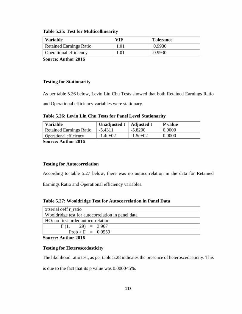
113
Table 5.25: Test for Multicollinearity
Variable VIF Tolerance
Retained Earnings Ratio 1.01 0.9930
Operational efficiency 1.01 0.9930
Source: Author 2016
Testing for Stationarity
As per table 5.26 below, Levin Lin Chu Tests showed that both Retained Earnings Ratio
and Operational efficiency variables were stationary.
Table 5.26: Levin Lin Chu Tests for Panel Level Stationarity
Variable Unadjusted t Adjusted t P value
Retained Earnings Ratio -5.4311 -5.8200 0.0000
Operational efficiency -1.4e+02 -1.5e+02 0.0000
Source: Author 2016
Testing for Autocorrelation
According to table 5.27 below, there was no autocorrelation in the data for Retained
Earnings Ratio and Operational efficiency variables.
Table 5.27: Wooldridge Test for Autocorrelation in Panel Data
xtserial oeff r_ratio
Wooldridge test for autocorrelation in panel data
HO: no first-order autocorrelation
F (1, 29) = 3.967
Prob > F = 0.0559
Source: Author 2016
Testing for Heteroscedasticity
The likelihood ratio test, as per table 5.28 indicates the presence of heteroscedasticity. This
is due to the fact that its p value was 0.0000<5%.
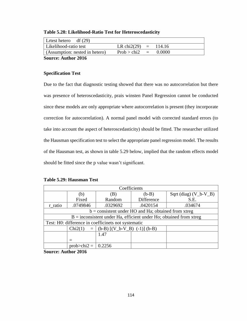
114
Table 5.28: Likelihood-Ratio Test for Heteroscedasticity
Lrtest hetero df (29)
Likelihood-ratio test LR chi2(29) = 114.16
(Assumption: nested in hetero) Prob > chi2 = 0.0000
Source: Author 2016
Specification Test
Due to the fact that diagnostic testing showed that there was no autocorrelation but there
was presence of heteroscedasticity, prais winsten Panel Regression cannot be conducted
since these models are only appropriate where autocorrelation is present (they incorporate
correction for autocorrelation). A normal panel model with corrected standard errors (to
take into account the aspect of heteroscedasticity) should be fitted. The researcher utilized
the Hausman specification test to select the appropriate panel regression model. The results
of the Hausman test, as shown in table 5.29 below, implied that the random effects model
should be fitted since the p value wasn’t significant.
Table 5.29: Hausman Test
Coefficients
(b)
Fixed
(B)
Random
(b-B)
Difference
Sqrt (diag) (V_b-V_B)
S.E.
r_ratio .0749846 .0329692 .0420154 .034674
b = consistent under HO and Ha; obtained from xtreg
B = inconsistent under Ha, efficient under Ho; obtained from xtreg
Test: H0: difference in coefficinets not systematic
Chi2(1) = (b-B) [(V_b-V_B) (-1)] (b-B)
=
1.47
prob>chi2 = 0.2256
Source: Author 2016
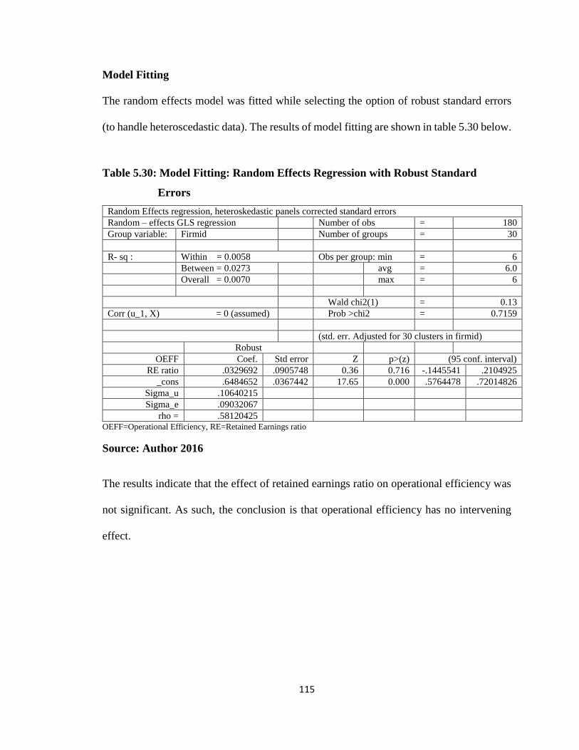
115
Model Fitting
The random effects model was fitted while selecting the option of robust standard errors
(to handle heteroscedastic data). The results of model fitting are shown in table 5.30 below.
Table 5.30: Model Fitting: Random Effects Regression with Robust Standard
Errors
Random Effects regression, heteroskedastic panels corrected standard errors
Random – effects GLS regression Number of obs = 180
Group variable: Firmid Number of groups = 30
R- sq : Within = 0.0058 Obs per group: min = 6
Between = 0.0273 avg = 6.0
Overall = 0.0070 max = 6
Wald chi2(1) = 0.13
Corr (u_1, X) = 0 (assumed) Prob >chi2 = 0.7159
(std. err. Adjusted for 30 clusters in firmid)
Robust
OEFF Coef. Std error Z p>(z) (95 conf. interval)
RE ratio .0329692 .0905748 0.36 0.716 -.1445541 .2104925
_cons .6484652 .0367442 17.65 0.000 .5764478 .72014826
Sigma_u .10640215
Sigma_e .09032067
rho = .58120425 OEFF=Operational Efficiency, RE=Retained Earnings ratio
Source: Author 2016
The results indicate that the effect of retained earnings ratio on operational efficiency was
not significant. As such, the conclusion is that operational efficiency has no intervening
effect.
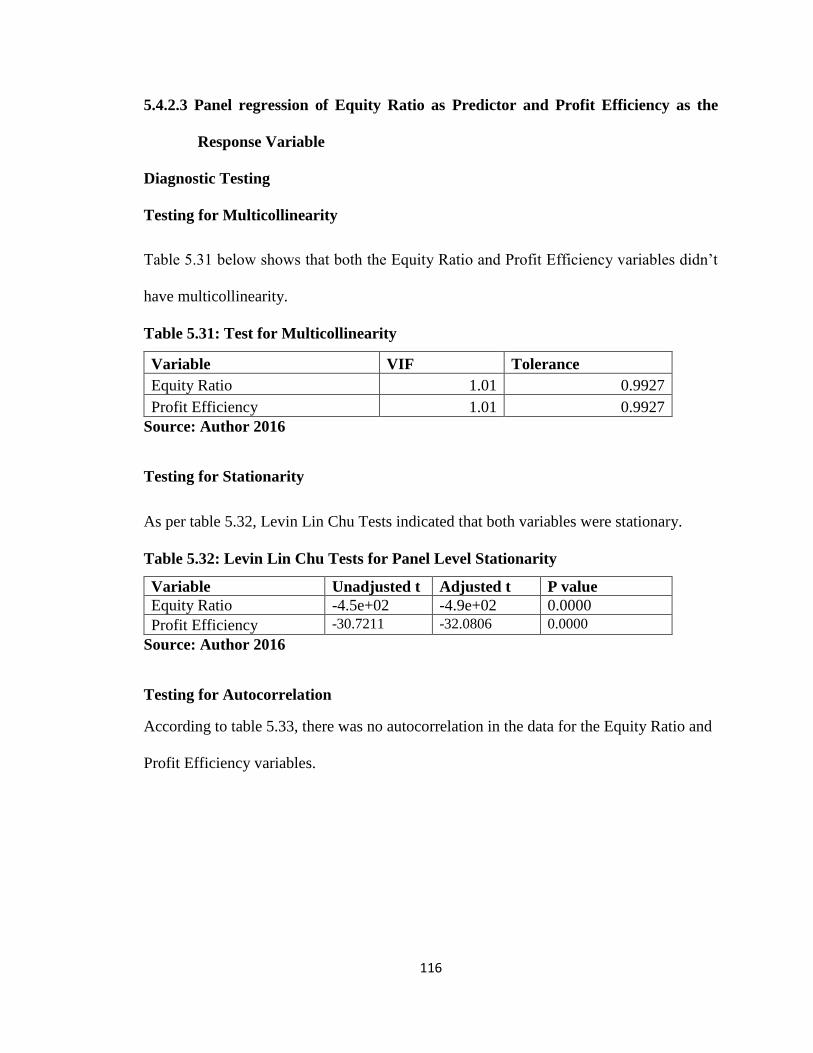
116
5.4.2.3 Panel regression of Equity Ratio as Predictor and Profit Efficiency as the
Response Variable
Diagnostic Testing
Testing for Multicollinearity
Table 5.31 below shows that both the Equity Ratio and Profit Efficiency variables didn’t
have multicollinearity.
Table 5.31: Test for Multicollinearity
Variable VIF Tolerance
Equity Ratio 1.01 0.9927
Profit Efficiency 1.01 0.9927
Source: Author 2016
Testing for Stationarity
As per table 5.32, Levin Lin Chu Tests indicated that both variables were stationary.
Table 5.32: Levin Lin Chu Tests for Panel Level Stationarity
Variable Unadjusted t Adjusted t P value
Equity Ratio -4.5e+02 -4.9e+02 0.0000
Profit Efficiency -30.7211 -32.0806 0.0000
Source: Author 2016
Testing for Autocorrelation
According to table 5.33, there was no autocorrelation in the data for the Equity Ratio and
Profit Efficiency variables.
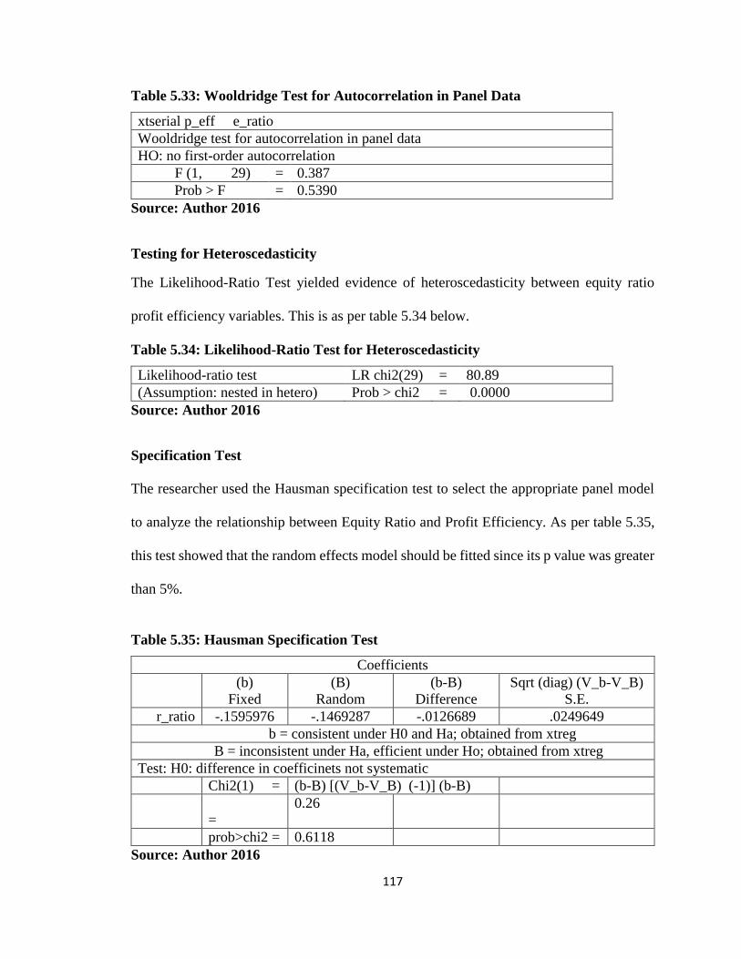
117
Table 5.33: Wooldridge Test for Autocorrelation in Panel Data
xtserial p_eff e_ratio
Wooldridge test for autocorrelation in panel data
HO: no first-order autocorrelation
F (1, 29) = 0.387
Prob > F = 0.5390
Source: Author 2016
Testing for Heteroscedasticity
The Likelihood-Ratio Test yielded evidence of heteroscedasticity between equity ratio
profit efficiency variables. This is as per table 5.34 below.
Table 5.34: Likelihood-Ratio Test for Heteroscedasticity
Likelihood-ratio test LR chi2(29) = 80.89
(Assumption: nested in hetero) Prob > chi2 = 0.0000
Source: Author 2016
Specification Test
The researcher used the Hausman specification test to select the appropriate panel model
to analyze the relationship between Equity Ratio and Profit Efficiency. As per table 5.35,
this test showed that the random effects model should be fitted since its p value was greater
than 5%.
Table 5.35: Hausman Specification Test
Coefficients
(b)
Fixed
(B)
Random
(b-B)
Difference
Sqrt (diag) (V_b-V_B)
S.E.
r_ratio -.1595976 -.1469287 -.0126689 .0249649
b = consistent under H0 and Ha; obtained from xtreg
B = inconsistent under Ha, efficient under Ho; obtained from xtreg
Test: H0: difference in coefficinets not systematic
Chi2(1) = (b-B) [(V_b-V_B) (-1)] (b-B)
=
0.26
prob>chi2 = 0.6118
Source: Author 2016
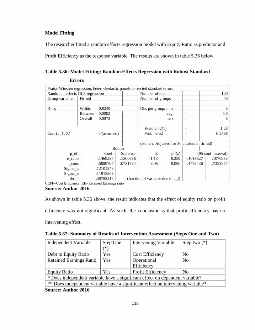
118
Model Fitting
The researcher fitted a random effects regression model with Equity Ratio as predictor and
Profit Efficiency as the response variable. The results are shown in table 5.36 below.
Table 5.36: Model Fitting: Random Effects Regression with Robust Standard
Errors
Praise-Winsten regression, heteroskedastic panels corrected standard errors
Random – effects GLS regression Number of obs = 180
Group variable: Firmid Number of groups = 30
R- sq : Within = 0.0249 Obs per group: min = 6
Between = 0.0002 avg = 6.0
Overall = 0.0073 max = 6
Wald chi2(1) = 1.28
Corr (u_1, X) = 0 (assumed) Prob >chi2 = 0.2586
(std. err. Adjusted for 30 clusters in firmid)
Robust
p_eff Coef. Std error Z p>(z) (95 conf. interval)
e_ratio -.1469287 .1300656 -1.13 0.259 -.4018527 .1079953
_cons .5889707 .0731784 8.05 0.000 .4455436 .7323977
Sigma_u .12101249
Sigma_e .11913368
rho = .50782315 (fraction of variance due to u_i) CEFF=Cost Efficiency, RE=Retained Earnings ratio
Source: Author 2016
As shown in table 5.36 above, the result indicates that the effect of equity ratio on profit
efficiency was not significant. As such, the conclusion is that profit efficiency has no
intervening effect.
Table 5.37: Summary of Results of Intervention Assessment (Steps One and Two)
Independent Variable Step One
(*)
Intervening Variable Step two (*)
Debt to Equity Ratio Yes Cost Efficiency No
Retained Earnings Ratio Yes Operational
Efficiency
No
Equity Ratio Yes Profit Efficiency No
* Does independent variable have a significant effect on dependent variable?
** Does independent variable have a significant effect on intervening variable?
Source: Author 2016
119
Table 5.37 above summarizes the results of intervention assessment. Since there is no
apparent effect of the independent variables on the intervening variables, the conclusion is
that there is no intervening effect and hence steps three and four are not necessary. In
hypothesis testing, we fail to reject null hypothesis three (H03). It is therefore concluded
that firm efficiency have no intervening effect on the relationship between capital structure
and firm value.
5.5 Joint Effect of Capital Structure, Macroeconomic Environment and Firm
Efficiency on the Value of the Firm
This part relates to the fourth objective of the study. The researcher tested the joint effect
of capital structure, macroeconomic environment and firm efficiency on the value of the
firm. Hypothesis four was framed in the null below:
H04: capital structure, macroeconomic environment and firm’s efficiency do not have a
significant joint influence on the value of the firm.
Diagnostic Tests
Testing for Multicollinearity
As per table 5.38 below, there was high multicollinearity of three independent variable
indicators initially but the indicators of the moderating variable and intervening variable
had acceptable VIFs. Retained Earnings Ratio, Equity Ratio, and Debt Ratio had very big
VIFs of 1051.27, 934.28, and 1646.73 respectively. Only Debt to equity Ratio had a VIF
which is less than 10. Consequently, Debt Ratio was removed from further analysis since
it had the highest VIF, meaning it had most collinearity with other variables.
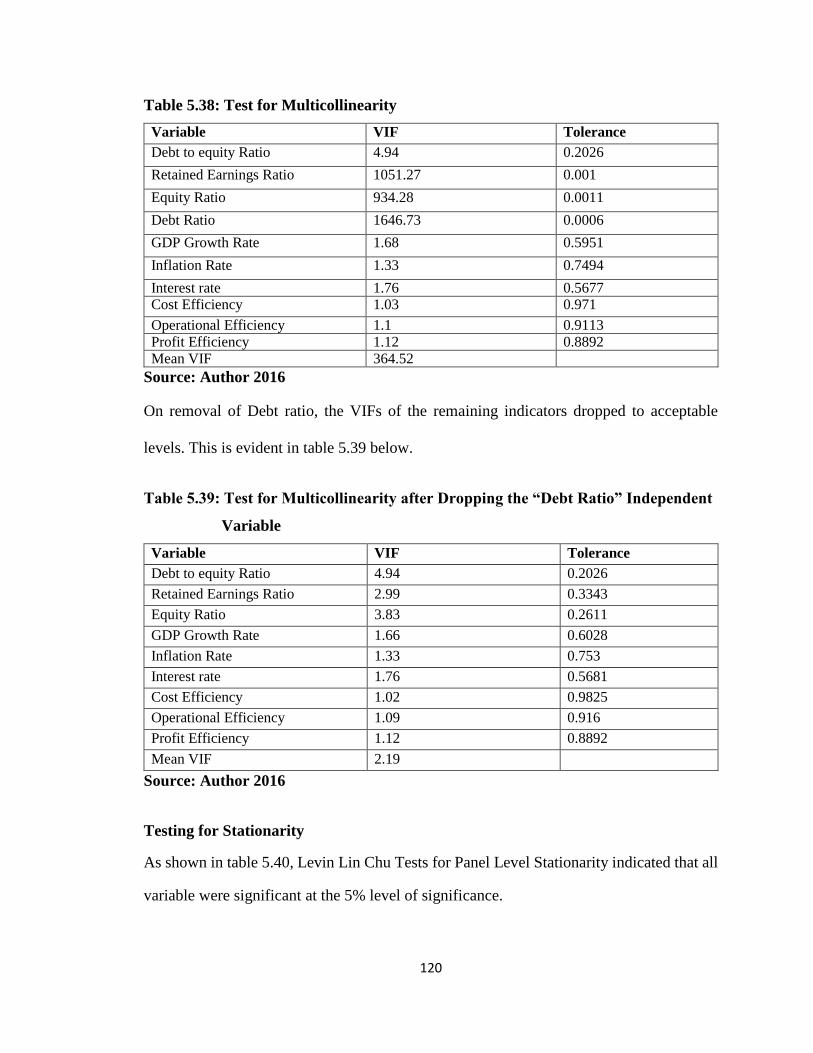
120
Table 5.38: Test for Multicollinearity
Variable VIF Tolerance
Debt to equity Ratio 4.94 0.2026
Retained Earnings Ratio 1051.27 0.001
Equity Ratio 934.28 0.0011
Debt Ratio 1646.73 0.0006
GDP Growth Rate 1.68 0.5951
Inflation Rate 1.33 0.7494
Interest rate 1.76 0.5677 Cost Efficiency 1.03 0.971
Operational Efficiency 1.1 0.9113
Profit Efficiency 1.12 0.8892
Mean VIF 364.52
Source: Author 2016
On removal of Debt ratio, the VIFs of the remaining indicators dropped to acceptable
levels. This is evident in table 5.39 below.
Table 5.39: Test for Multicollinearity after Dropping the “Debt Ratio” Independent
Variable
Variable VIF Tolerance
Debt to equity Ratio 4.94 0.2026
Retained Earnings Ratio 2.99 0.3343
Equity Ratio 3.83 0.2611
GDP Growth Rate 1.66 0.6028
Inflation Rate 1.33 0.753
Interest rate 1.76 0.5681
Cost Efficiency 1.02 0.9825
Operational Efficiency 1.09 0.916
Profit Efficiency 1.12 0.8892
Mean VIF 2.19
Source: Author 2016
Testing for Stationarity
As shown in table 5.40, Levin Lin Chu Tests for Panel Level Stationarity indicated that all
variable were significant at the 5% level of significance.
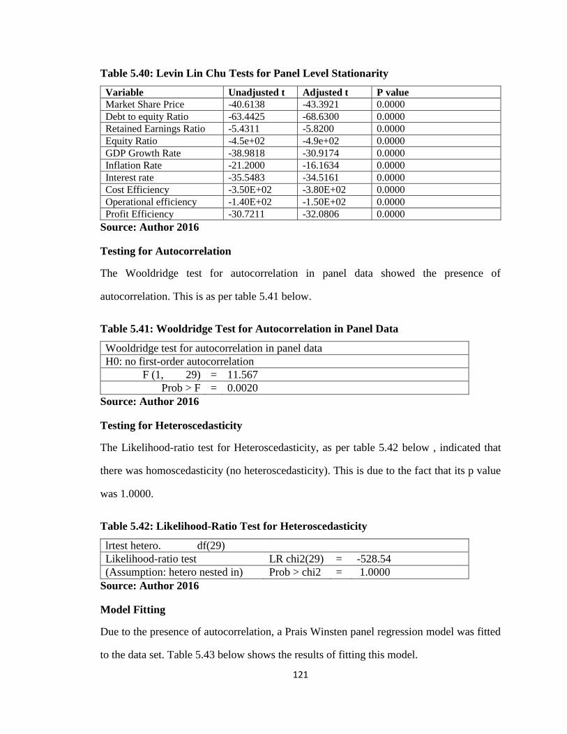
121
Table 5.40: Levin Lin Chu Tests for Panel Level Stationarity
Variable Unadjusted t Adjusted t P value
Market Share Price -40.6138 -43.3921 0.0000
Debt to equity Ratio -63.4425 -68.6300 0.0000
Retained Earnings Ratio -5.4311 -5.8200 0.0000
Equity Ratio -4.5e+02 -4.9e+02 0.0000
GDP Growth Rate -38.9818 -30.9174 0.0000
Inflation Rate -21.2000 -16.1634 0.0000
Interest rate -35.5483 -34.5161 0.0000
Cost Efficiency -3.50E+02 -3.80E+02 0.0000
Operational efficiency -1.40E+02 -1.50E+02 0.0000
Profit Efficiency -30.7211 -32.0806 0.0000
Source: Author 2016
Testing for Autocorrelation
The Wooldridge test for autocorrelation in panel data showed the presence of
autocorrelation. This is as per table 5.41 below.
Table 5.41: Wooldridge Test for Autocorrelation in Panel Data
Wooldridge test for autocorrelation in panel data
H0: no first-order autocorrelation
F (1, 29) = 11.567
Prob > F = 0.0020
Source: Author 2016
Testing for Heteroscedasticity
The Likelihood-ratio test for Heteroscedasticity, as per table 5.42 below , indicated that
there was homoscedasticity (no heteroscedasticity). This is due to the fact that its p value
was 1.0000.
Table 5.42: Likelihood-Ratio Test for Heteroscedasticity
lrtest hetero. df(29)
Likelihood-ratio test LR chi2(29) = -528.54
(Assumption: hetero nested in) Prob > chi2 = 1.0000
Source: Author 2016
Model Fitting
Due to the presence of autocorrelation, a Prais Winsten panel regression model was fitted
to the data set. Table 5.43 below shows the results of fitting this model.
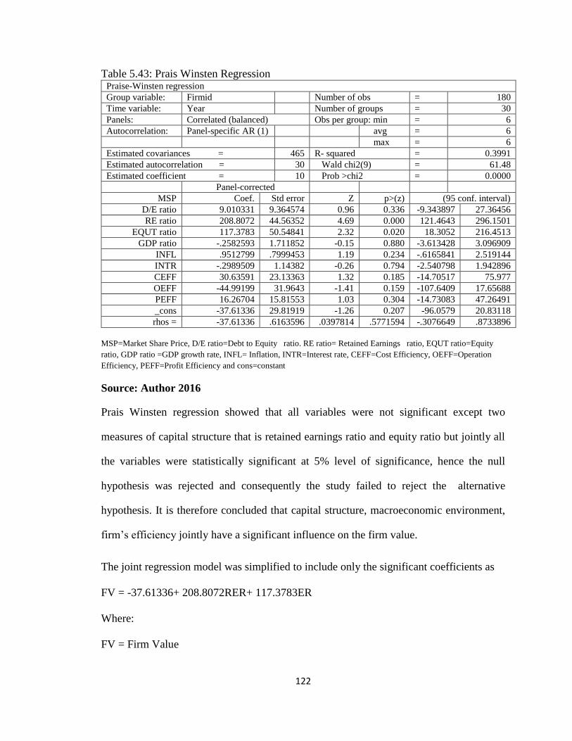
122
Table 5.43: Prais Winsten Regression Praise-Winsten regression
Group variable: Firmid Number of obs = 180
Time variable: Year Number of groups = 30
Panels: Correlated (balanced) Obs per group: min = 6
Autocorrelation: Panel-specific AR (1) avg = 6
max = 6
Estimated covariances = 465 R- squared = 0.3991
Estimated autocorrelation = 30 Wald chi2(9) = 61.48
Estimated coefficient = 10 Prob >chi2 = 0.0000
Panel-corrected
MSP Coef. Std error Z p>(z) (95 conf. interval)
D/E ratio 9.010331 9.364574 0.96 0.336 -9.343897 27.36456
RE ratio 208.8072 44.56352 4.69 0.000 121.4643 296.1501
EQUT ratio 117.3783 50.54841 2.32 0.020 18.3052 216.4513
GDP ratio -.2582593 1.711852 -0.15 0.880 -3.613428 3.096909
INFL .9512799 .7999453 1.19 0.234 -.6165841 2.519144
INTR -.2989509 1.14382 -0.26 0.794 -2.540798 1.942896
CEFF 30.63591 23.13363 1.32 0.185 -14.70517 75.977
OEFF -44.99199 31.9643 -1.41 0.159 -107.6409 17.65688
PEFF 16.26704 15.81553 1.03 0.304 -14.73083 47.26491
_cons -37.61336 29.81919 -1.26 0.207 -96.0579 20.83118
rhos = -37.61336 .6163596 .0397814 .5771594 -.3076649 .8733896
MSP=Market Share Price, D/E ratio=Debt to Equity ratio. RE ratio= Retained Earnings ratio, EQUT ratio=Equity
ratio, GDP ratio =GDP growth rate, INFL= Inflation, INTR=Interest rate, CEFF=Cost Efficiency, OEFF=Operation
Efficiency, PEFF=Profit Efficiency and cons=constant
Source: Author 2016
Prais Winsten regression showed that all variables were not significant except two
measures of capital structure that is retained earnings ratio and equity ratio but jointly all
the variables were statistically significant at 5% level of significance, hence the null
hypothesis was rejected and consequently the study failed to reject the alternative
hypothesis. It is therefore concluded that capital structure, macroeconomic environment,
firm’s efficiency jointly have a significant influence on the firm value.
The joint regression model was simplified to include only the significant coefficients as
FV = -37.61336+ 208.8072RER+ 117.3783ER
Where:
FV = Firm Value
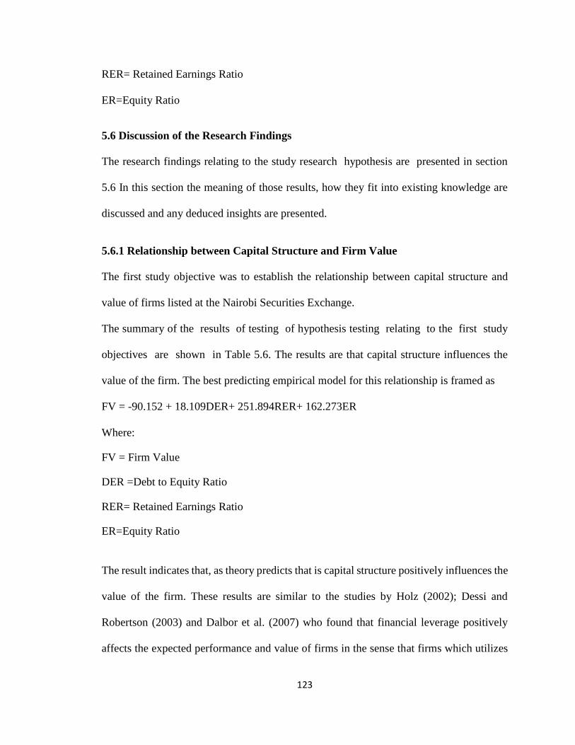
123
RER= Retained Earnings Ratio
ER=Equity Ratio
5.6 Discussion of the Research Findings
The research findings relating to the study research hypothesis are presented in section
5.6 In this section the meaning of those results, how they fit into existing knowledge are
discussed and any deduced insights are presented.
5.6.1 Relationship between Capital Structure and Firm Value
The first study objective was to establish the relationship between capital structure and
value of firms listed at the Nairobi Securities Exchange.
The summary of the results of testing of hypothesis testing relating to the first study
objectives are shown in Table 5.6. The results are that capital structure influences the
value of the firm. The best predicting empirical model for this relationship is framed as
FV = -90.152 + 18.109DER+ 251.894RER+ 162.273ER
Where:
FV = Firm Value
DER =Debt to Equity Ratio
RER= Retained Earnings Ratio
ER=Equity Ratio
The result indicates that, as theory predicts that is capital structure positively influences the
value of the firm. These results are similar to the studies by Holz (2002); Dessi and
Robertson (2003) and Dalbor et al. (2007) who found that financial leverage positively
affects the expected performance and value of firms in the sense that firms which utilizes
124
debts to finance assets and operations benefits from tax shields advantage by protecting
firm profit from taxation and invests the protected earnings in the growth of the firm
impacting in the future market value of the firm shares. However the results contradicts
studies by Majumdar and Chibber (1997); Abor (2005); Kadongo, Mokoteli and Mwangi
(2014) and Mwangi, Makau and Kosimbei (2014) who had found negative relationship
between debt equity ratio and the value of the firm
5.6.2 Moderating Influence of Macroeconomic Environment in the Relationship
between Capital Structure and Firm Value
The second study objective was to determine the moderating effect of the macroeconomic
environment on the relationship between capital structure and firm value. The summary of
the results of testing of hypothesis relating to the second study objective are shown in Table
5.12. In the first step of estimating the joint effect of independent variable and moderating
variable on dependent variable, the results of regression analysis show that retained
earnings ratio (b=247.111, p=0.000) and equity ratio (b=154.896, p=0.000) had a positive
significant relationship with firm value. The constant also had a significant but negative
relationship with firm value (b=-87.747, p=0.028). Debt to equity ratio (b=16.654,
p=0.064) and inflation rate (b=0.961, p=0.0330) had a positive but insignificant effect on
firm value while the effect of GDP growth rate (b=-0.046, p=0.985) and Interest Rate (b=-
0.482, p=0.766) on firm value was negative and insignificant. The R-squared was 0.3692.
This implies that 36.92% of variability in firm value could be attributed to variability in
capital structure and macroeconomic environment. On testing the effect of the interaction
terms, GDP Growth Rate had a significant interaction effect on Retained Earnings Ratio;
Interest Rate had a significant interaction effect on Retained Earnings Ratio and Earnings
125
Ratio; while Inflation Rate had a significant interaction effect on Earnings Ratio.The R-
squared was 0.4116. This implies that 41.16 % of variability in firm value could be
attributed to interaction effect of capital structure and macroeconomic environment.
The results of analysis indicate that , there is interaction between capital structure and
macroeconomic environment which contributed to the change of variation of firm value
by 0.0424(0.4116-0.3692)..The best predicting empirical model for this relationship is
framed as
FV=31.93675+4.49967INL-6.495636INTR+67.35739
IT2+38.51985IT5+58.29853IT6+17.62323IT9
Where:
FV = Firm Value
INFL =Inflation
INTR= Interest
IT2= GDP Growth rate and Retained Earnings ratio interaction term
IT5 =Inflation rate and Retained Earnings ratio interaction term
IT6= Inflation rate and Equity ratio interaction term
IT9=Interest rate and Equity ratio interaction term
The study finding is consistent with the results by Fanelli and Keifman (2002) who
argued that the country’s financial markets , unstable economic environment and
external events have effects on investment decisions of companies. This implies issuance
of stocks by companies for financing is suitable only when the country is in good economic
situations due to the fact that during the given periods the firms are able to issue shares at
favourable terms which affects their overall firm value .The findings are also consistent
126
with the studies by Cheng and Tzeng (2011) who indicated that the higher firm quality
may improve firm credit rationing by debt holders and equity holders depending on the
economic environment prevailing in the country and better credit rating resulted in a
reduced cost of capital and the reduced cost of obtaining finances in the market impacting
on the firm operational costs, profits and dividends to be paid to the owners ultimately
influencing the firm market share price. It is worth to note that none of the above studies
had considered macroeconomic environment as a moderating variable but rather had
considered the pairwise relationship between macroeconomic environment and firm value
or between capital structure and macroeconomic environment
5.6.3 Intervening Effects of Firm’s efficiency in the Relationship between Capital
Structure and Firm Value
The third study objective was to ascertain the intervening effects of firm’s efficiency
(operational, cost and profit efficiency) on the relationship between capital structure and
firm value.
As presented in Tables 5.15 and 5.16 there is a no statistically significant relationship
between capital structure, firm efficiency and value, which leads to the conclusion that
there is no significant joint effect of capital structure, firm efficiency and value of firms
listed at the Nairobi Securities Exchange. This finding thus leads to the failure to reject
hypothesis three (H03) and rejected alternative hypothesis. This finding is inconsistent with
empirical arguments by Schumpeter (1934): Greene and Segal (2004); Callen et al. (2005):
Cummins and Xie (2008) and Norman, Hatfield & Cardinal (2010) which had found firm
efficiency to have an influence on the firm value. However, the findings of the current
studies are inconsistent with other studies which reported a negative relationship
127
between capital structure, firm productivity in terms of efficiency and firm value which
includes studies by Pushner (1995) who found negative effect of leverage on firm
performance measured as total factor productivity (TFP) in Japan. Booth et al (2001) in
their study of 10 developing countries who found a negative relation between leverage and
firm performance and firm value and Onaolapo and Kajola (2010) who found a significant
negative impact of leverage, total factor productivity (TFP) on financial measures of
Nigeria firms.
The concept of capital structure, firm efficiency and value have not been previously
considered together as has been done in this study. The previous studies had looked at
two variables that is firm efficiency and value at a time and thereby ignoring the joint
effects of all three variables considered together.
5.6.4 Joint Effects of Capital Structure, Macroeconomic Environment, Firm’s
efficiency and Firm Value
The fourth study objective was to determine the joint effects of capital structure,
macroeconomic environment, firm efficiency and firm value. The summary of the results
of testing of the fourth research hypothesis relating to this study objective in Table 5.43
showed that all variables were not significant except two measures of capital structure that
is retained earnings ratio and equity ratio but jointly all the variables were statistically
significant at 5% level of significance, hence the null hypothesis was rejected and
consequently the study failed to reject alternative hypothesis. It is therefore concluded that
capital structure, macroeconomic environment, firm’s efficiency jointly have a significant
influence on the firm value. The best predicting empirical model for this relationship is
framed as

128
FV = -37.61336 + 18.109DER+ 208.8072RER+ 117.3783ER
Where:
FV = Firm Value
RER= Retained Earnings Ratio
ER=Earnings Ratio
The concepts of capital structure, macroeconomic environment, firm efficiency and value
have not been previously considered together as has been done in this study. However the
result is consistent with the results from pairwise previous studies by Holz (2002); Dessi
and Robertson (2003) and Dopuch and Gupta (1997) whereby a positive and significant
relationship between the firm choice of capital and its return on assets return on equity and
market share price was evidenced. Additionally Cheng and Tzeng (2011) supported the
study findings by indicating that the higher the firm quality emerging from operational
efficiency may improve firm credit rationing by debt holders and equity holders depending
on the macroeconomic environment prevailing in the country. Their study concluded that
better credit rationing resulted in a reduced cost of capital and increased firm value.
5.7 Chapter Summary
The chapter started with testing of the study hypotheses followed by discussion of the
results of hypothesis testing . For each of the four hypotheses, analysis started with the
conducting of diagnostic testing to appraise the conformance of the data with assumptions
of Ordinary Least Squares (OLS) panel regression analysis. This was to enable the
researcher to use robust models that are an exact fit for the data’s attributes thereby
preventing the probability of making either a type 1 error (rejecting a correct null
hypothesis) or a type 2 error (failing to reject an incorrect null hypothesis).The summary
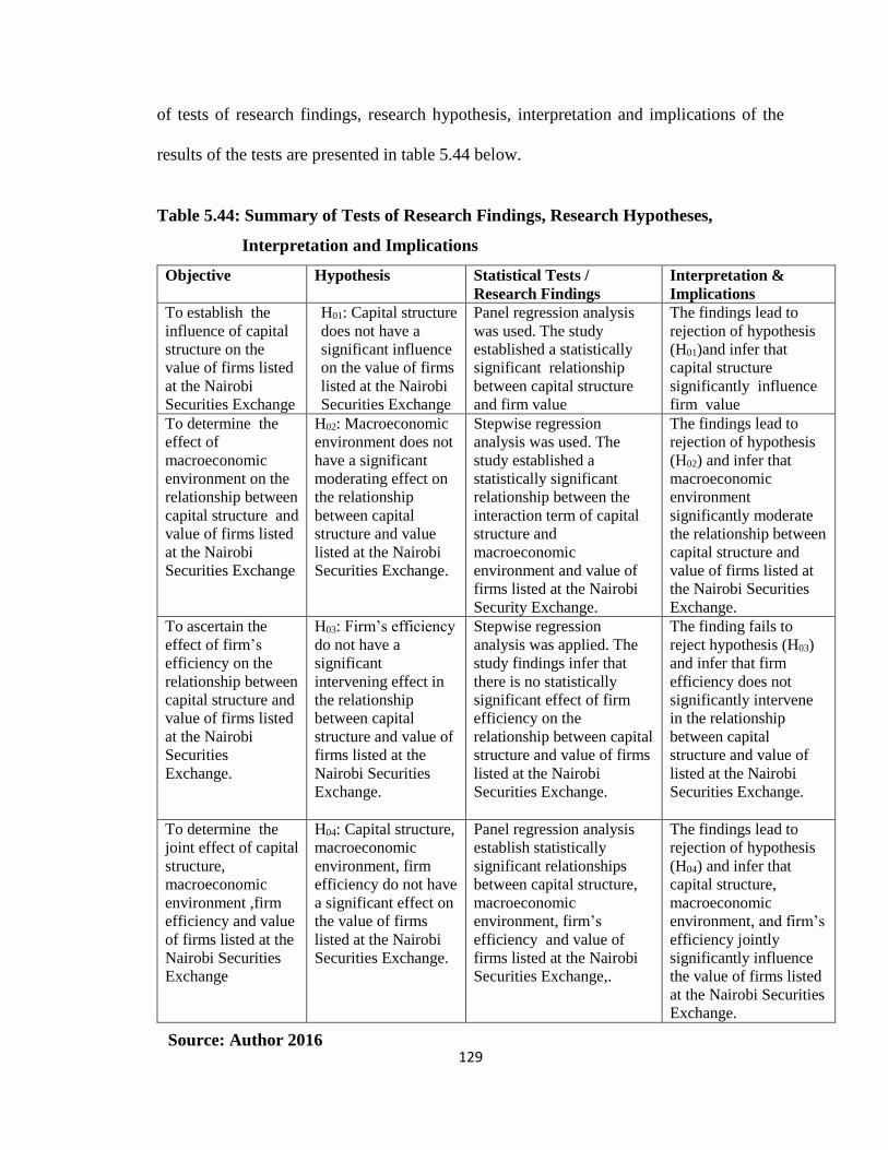
129
of tests of research findings, research hypothesis, interpretation and implications of the
results of the tests are presented in table 5.44 below.
Table 5.44: Summary of Tests of Research Findings, Research Hypotheses,
Interpretation and Implications
Objective Hypothesis Statistical Tests /
Research Findings
Interpretation &
Implications
To establish the
influence of capital
structure on the
value of firms listed
at the Nairobi
Securities Exchange
H01: Capital structure
does not have a
significant influence
on the value of firms
listed at the Nairobi
Securities Exchange
Panel regression analysis
was used. The study
established a statistically
significant relationship
between capital structure
and firm value
The findings lead to
rejection of hypothesis
(H01)and infer that
capital structure
significantly influence
firm value
To determine the
effect of
macroeconomic
environment on the
relationship between
capital structure and
value of firms listed
at the Nairobi
Securities Exchange
H02: Macroeconomic
environment does not
have a significant
moderating effect on
the relationship
between capital
structure and value
listed at the Nairobi
Securities Exchange.
Stepwise regression
analysis was used. The
study established a
statistically significant
relationship between the
interaction term of capital
structure and
macroeconomic
environment and value of
firms listed at the Nairobi
Security Exchange.
The findings lead to
rejection of hypothesis
(H02) and infer that
macroeconomic
environment
significantly moderate
the relationship between
capital structure and
value of firms listed at
the Nairobi Securities
Exchange.
To ascertain the
effect of firm’s
efficiency on the
relationship between
capital structure and
value of firms listed
at the Nairobi
Securities
Exchange.
H03: Firm’s efficiency
do not have a
significant
intervening effect in
the relationship
between capital
structure and value of
firms listed at the
Nairobi Securities
Exchange.
Stepwise regression
analysis was applied. The
study findings infer that
there is no statistically
significant effect of firm
efficiency on the
relationship between capital
structure and value of firms
listed at the Nairobi
Securities Exchange.
The finding fails to
reject hypothesis (H03)
and infer that firm
efficiency does not
significantly intervene
in the relationship
between capital
structure and value of
listed at the Nairobi
Securities Exchange.
To determine the
joint effect of capital
structure,
macroeconomic
environment ,firm
efficiency and value
of firms listed at the
Nairobi Securities
Exchange
H04: Capital structure,
macroeconomic
environment, firm
efficiency do not have
a significant effect on
the value of firms
listed at the Nairobi
Securities Exchange.
Panel regression analysis
establish statistically
significant relationships
between capital structure,
macroeconomic
environment, firm’s
efficiency and value of
firms listed at the Nairobi
Securities Exchange,.
The findings lead to
rejection of hypothesis
(H04) and infer that
capital structure,
macroeconomic
environment, and firm’s
efficiency jointly
significantly influence
the value of firms listed
at the Nairobi Securities
Exchange.
Source: Author 2016
130
CHAPTER SIX
SUMMARY, CONCLUSIONS AND RECOMMENDATIONS
6.1 Introduction
This chapter contains a summary of the findings, conclusions and recommendations. The
study set out to establish the relationship among capital structure, macroeconomic
environment, firm efficiency and value of firms listed at the Nairobi Securities Exchange
by testing four hypotheses that explored the four variables. The chapter presents the
summary of findings from descriptive statistics for each variable, conclusions from these
findings, study contributions and policy recommendations.The chapter also identifies the
limitation of the study and future research directions.
6.2 Summary of the Study
The main objective of this study was to establish the effect of capital structure on the value
of the firm. The study further analysed the influence of macroeconomic environment and
firm efficiency on the relationship between capital structure and firm value. The study was
anchored on MM theory of capital structure and used positivistic philosophy in testing four
research hypothesis. The study utilized secondary data from non- financial firms listed at
the Nairobi Securities Exchange. Further the study employed a descriptive longitudinal
research design and used panel data analysis based on the Ordinary least squares model.
The population of the study was 62 companies listed at the Nairobi Securities
Exchange .Out of 42 non-financial institutions listed at the Nairobi Securities Exchange
that the study initially targeted complete data was available for 30 companies. As such, the
sample consisted of 30 non-financial institutions that traded consistently over the 2009 to
2014 period and whose data was available.

131
There was a relatively strongly negative correlation between debt to equity ratio and market
share price. The correlation between retained earnings ratio was quite strong (r=0.387)
while the effect of equity ratio on market share price was relatively weak and insignificant
at both 5% and 1% levels of significance. The strong, positive and significant correlation
between retained earnings and market share price can be attributed to many factors. Most
important of all, firms with high retention rates are viewed by the market as growth firms
with huge prospects for the future. Finally, Debt Ratio and market share price had a
relatively strongly, negative correlation (r = -.392). The negative effect of the debt to equity
ratio and debt ratio on the market share price showed a strong preference on unlevered
stocks by investors. Due to mandatory interest and principal repayments, highly indebted
firms tend to have less amounts of money that are available for distribution as dividends.
Additionally, debt could send a signal that the financial health of a firm is in turmoil,
thereby making it less attractive to investors.
For each of the four hypotheses, empirical analysis started with the conducting of
diagnostic testing to appraise the conformance of the data with assumptions of Ordinary
Least Squares (OLS) panel regression analysis and in situations where diagnostics tests
revealed non-conformance with the assumptions of Ordinary Least Squares (OLS) panel
regression analysis, Prais Winsten Panel Regression with corrected standard errors model
was used. This was to enable the researcher to use robust models that are an exact fit for
the data’s attributes thereby preventing the probability of making either a type 1 error
(rejecting a correct null hypothesis) or a type 2 error (failing to reject an incorrect null
hypothesis).
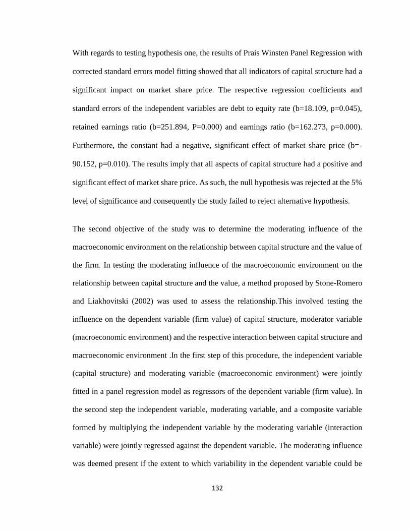
132
With regards to testing hypothesis one, the results of Prais Winsten Panel Regression with
corrected standard errors model fitting showed that all indicators of capital structure had a
significant impact on market share price. The respective regression coefficients and
standard errors of the independent variables are debt to equity rate (b=18.109, p=0.045),
retained earnings ratio (b=251.894, P=0.000) and earnings ratio (b=162.273, p=0.000).
Furthermore, the constant had a negative, significant effect of market share price (b=-
90.152, p=0.010). The results imply that all aspects of capital structure had a positive and
significant effect of market share price. As such, the null hypothesis was rejected at the 5%
level of significance and consequently the study failed to reject alternative hypothesis.
The second objective of the study was to determine the moderating influence of the
macroeconomic environment on the relationship between capital structure and the value of
the firm. In testing the moderating influence of the macroeconomic environment on the
relationship between capital structure and the value, a method proposed by Stone-Romero
and Liakhovitski (2002) was used to assess the relationship.This involved testing the
influence on the dependent variable (firm value) of capital structure, moderator variable
(macroeconomic environment) and the respective interaction between capital structure and
macroeconomic environment .In the first step of this procedure, the independent variable
(capital structure) and moderating variable (macroeconomic environment) were jointly
fitted in a panel regression model as regressors of the dependent variable (firm value). In
the second step the independent variable, moderating variable, and a composite variable
formed by multiplying the independent variable by the moderating variable (interaction
variable) were jointly regressed against the dependent variable. The moderating influence
was deemed present if the extent to which variability in the dependent variable could be
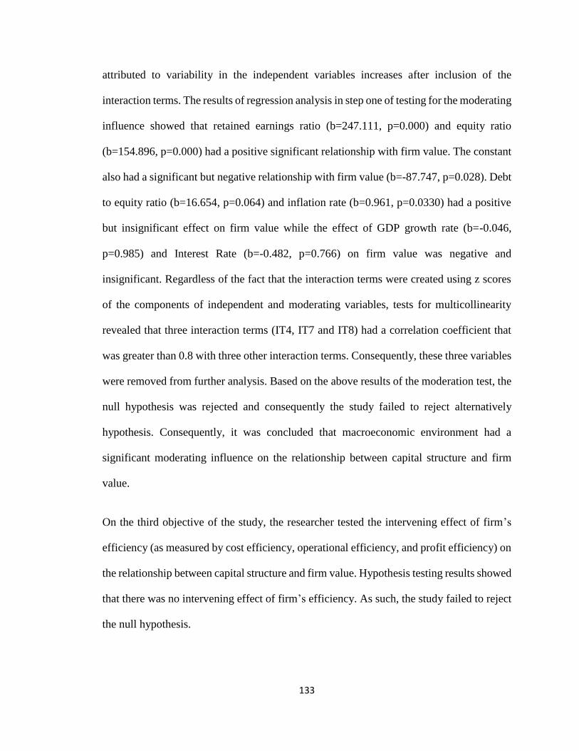
133
attributed to variability in the independent variables increases after inclusion of the
interaction terms. The results of regression analysis in step one of testing for the moderating
influence showed that retained earnings ratio (b=247.111, p=0.000) and equity ratio
(b=154.896, p=0.000) had a positive significant relationship with firm value. The constant
also had a significant but negative relationship with firm value (b=-87.747, p=0.028). Debt
to equity ratio (b=16.654, p=0.064) and inflation rate (b=0.961, p=0.0330) had a positive
but insignificant effect on firm value while the effect of GDP growth rate (b=-0.046,
p=0.985) and Interest Rate (b=-0.482, p=0.766) on firm value was negative and
insignificant. Regardless of the fact that the interaction terms were created using z scores
of the components of independent and moderating variables, tests for multicollinearity
revealed that three interaction terms (IT4, IT7 and IT8) had a correlation coefficient that
was greater than 0.8 with three other interaction terms. Consequently, these three variables
were removed from further analysis. Based on the above results of the moderation test, the
null hypothesis was rejected and consequently the study failed to reject alternatively
hypothesis. Consequently, it was concluded that macroeconomic environment had a
significant moderating influence on the relationship between capital structure and firm
value.
On the third objective of the study, the researcher tested the intervening effect of firm’s
efficiency (as measured by cost efficiency, operational efficiency, and profit efficiency) on
the relationship between capital structure and firm value. Hypothesis testing results showed
that there was no intervening effect of firm’s efficiency. As such, the study failed to reject
the null hypothesis.
134
The fourth study objective was to determine the joint effects of capital structure,
macroeconomic environment, firm efficiency and firm value. The summary of the results
of testing of the fourth research hypothesis relating to this study objective showed that all
variables were not significant except two measures of capital structure that is retained
earnings ratio and equity ratio but jointly all the variables were statistically significant at
5% level of significance, hence the null hypothesis was rejected and the study failed to
reject the alternative hypothesis. It was therefore concluded that capital structure,
macroeconomic environment, firm’s efficiency jointly have a significant influence on the
firm value.
6.3 Conclusions of the Study
The results obtained from the tests of hypothesis for the first study objective showed that
all aspects of capital structure had a positive and significant effect of market share price.
Consequently, it was concluded that capital structure had a significant influence of the
value of the firm and that 37.5 % of variability in firm value was attributed to variability
in capital structure. The results in the second study objective showed that conditions for
the existence of moderation were fulfilled in that macroeconomic environment moderated
the relationship between capital structure and firm value. The interaction effect of capital
structure and macroeconomic environment showed that the R-squared had improved
from 0.369 in the first step of moderation to 0.4116 in step two a change of 0.0424(0.4116-
0.3692).The results showed that variability in firm value could be attributed to the
interaction effect between capital structure and macroeconomic environment.
135
Results of the study objective number three indicated that firm’s efficiency did not
intervene in the relationship between capital structure and firm value. The study had
hypothesized that firm efficiency would significantly and positively influence the resultant
firm market share price. This means that the availability of finances either from retained
earnings, debt or equity to finance firm investments and operations determines whether the
firm has resources to undertake improvements in the firm core processes resulting to
efficiencies in firm’s operations. Typically to obtain firm efficiencies in its core processes
requires financial investments leading to heavy overall operations costs. As the operation
costs increases there is likelihood of decrease in firm profits when the firm revenues are
compared against the firm costs. Such a situation is likely to lead to reduced earnings,
dividends to the owners of the firm and a decline in the firm market share price in the short
run since the firm share price is information driven. The situation could reverse in the long
run when the firm attains optimum efficiency gained from the initial investments in the
improvements of its core processes and bounce back to profitability culminating with
enhanced firm market share price. The efficiency with which firm resources are managed
determines the competitiveness of the firm and hence the Kenyan firm manager should
focus on complete description of the economic goals of the firms aimed at reducing the
cost of inputs and maximize on the prices charged on the output (cost efficiency). This can
only be achieved through efficient utilization of firm resources in a cost effective manner
in order to maximize the firm revenues that impacts on the firm profit and eventually the
firm market share price.
The results of the fourth study objective showed that capital structure, macroeconomic
environment and firm efficiencies jointly had a statistically significant impact on the firm
value in the sense that optimal capital structure combined with optimal efficiencies in the

136
firm core processes under a favourable macroeconomic environment positively impacts on
the resultant firm market share price .However, the effect of the macroeconomic
environment and firm efficiencies when taken individually was not significant.
6.4 Contributions of the Study Findings
The findings from this study contribute to the body of knowledge in the area of capital
structure, macroeconomic environment, firm efficiency and value. This section highlights
the study findings contribution to knowledge and benefits to Kenyan companies practice
and policy.
6.4.1 Contributions to Knowledge
The results of this study add to existing knowledge in the area of capital structure,
macroeconomic environment, firm’s efficiency and firm value in three main ways:
First, the results of data analysis indicate that firms are relying more on equity capital than
retained earnings and debt with the pecking order being equity, retained earnings and debt.
This means Kenyans firms are not taking advantage of tax shields benefits which arise from
debt components in their capital structure. Kenyan firms should take advantage of tax
shield benefits by using more debt in their capital structure and benefits from displinary
role of debts which forces firm managers to manage the firm efficiently resulting to high
values for their firms. At the same time firm managers should be cautious of level of
indebtness in their firms since higher levels of debts can significantly decrease the firm’s
net profit causing a drop in the stock price. An optimum level of both debt and equity is
preferable inoder to benefits from tax shields and influence and control in the management
decisions through equity holder’s representations in the board of directors driving up the
firm’s value.
137
The second contribution of this study is the test of the moderating influence of
macroeconomic environment on the relationship between capital structure and firm value.
The findings of this study indicate that capital structure, macroeconomic environment have
a significant interaction effect on the firm value. Therefore the government has an
obligation to regulate the financial sector through various fiscal and monetary policy
interventions for the economy to support cost effective financing, this will positively
impacts on the revenues , profitability and the resulting market values of Kenyan firms.
Third contribution is that Kenyan firms should make practical application of agency costs
theory which postulates that financial leverage mitigates against the agency problems by
using debts in their capital structure as a displinary mechanisms forcing corporate
managers to operate their firms efficiently to enhance revenue generations to be used for
paying mandatory principle and interest on the borrowed funds. Additionally equity holders
should also play their role of exerting influence in managerial decisions towards improving
efficiency in the operations and prevent wastages of free cash-flow of their firms through
equity holders’ representation in the board of directors. Further firm managers should
continuously review past strategic decisions and incase those decisions were harmful to the
firm, make a deliberate move to correct the situations. The combined approach is expected
to enhance the value of Kenyan firms.
Finally this study extends capital structure firm value literature by demonstrating that the
relationship is not direct but is rather moderated by macroeconomic environment and in
some instances intervened by firm efficiency as long as well arraigned strategic choices
were made in the formulations of the capital structure decisions. This can explain why
many researchers who have tested the relationship between capital structure and firm value
138
have found contradictory results with some concluding the relationship between the
variables to be positive, negative or not significant at all. This study is important since it
has provided direction on how to integrate optimal financing strategy, efficient
management of firm’s resources utilizing the opportunities provided by a favourable macro
economic environment in order to realise enhanced values of Kenyan firms.Further, the
adverse effects as a result of unfavourable macroeconomic environment can be mitigated
through practical application of agency cost theory by improving efficiencies in
management of firm’s resources resulting to sustained firm’s value.
6.4.2 Contributions to Managerial Policy and Practices
The findings of this study are useful to various stakeholders including investors, corporate
managers, regulators and the government.
The effects of capital structure on firm value as documented in this study help investors
and corporate managers when financing their firm investment and operations. The
corporate managers should increase use of debt capital when financing their firm
investment and operations in order to maximize the tax shield benefits available to their
firms. The use of debt capital also provides displinary mechanisms to firm’s managers to
manage the firm’s resources efficiently. Equity holders on their part should play their
rightful role of exerting influence and monitoring managerial decisions through their
representation in the board of directors leading to higher value of their firms. Equity holders
can also sacrifice current dividends (capitalization-RE) providing funds for firm’s
investment to generate better returns in future in order to improve value of their firms.
139
Based on the results of this study the government through Capital Markets Authority
(CMA) and other stakeholders in the Kenyan corporate sector should develop appropriate
policies in an attempt to organize the debt capital market to enable Kenyan corporate
bodies get access to low cost long term debt capital to finance their investments and
operations. It is important to establish appropriate trading rules and mechanisms to
improve the efficiency of debt market as higher liquidity in secondary market generally
reduces the cost of capital which will positively impacts in the value of Kenyan firms.
The current study has revealed that Kenyan firms are relying more on costly equity finances
instead of debt financing locking themselves out of the tax shields benefits meant to
enhance the value of the firms listed at the Nairobi Securities Exchange.
The finding of this study is expected to guide managerial practitioners in the corporate
sector to appreciate the linkage of the various financing methods and efficient management
of firm’s resource and also actualize practical application of agency cost theory in the
management of their firm’s affairs including but not limited to efficient management of
firm resources. The government on the other hand has an obligation to provide stability of
the macroeconomic environment through its fiscal and monetary interventions. This
ensures low inflation rate, low tax rate, and high economic growth rate. Consequently, the
cost of operational expenses will decline and firm profits increase. This causes the value
of the firm to increase through a higher share price arising from higher dividends to
shareholders. The findings of this study is expected to inform corporate managers on how
to take advantage of the stable macroeconomic environment prevailing in the country and
in some instances how to mitigate the adverse effects of unstable macroeconomic
environment through increasing their cost efficiency and operational efficiency. The results

140
of the current study demonstrate that the firms are using more inputs for a unit of output
compared to the best firm. Therefore, firm managers should sell their products at higher
prices to break even especially when the firm outputs are not competitive in the market.
The consequences of failing to do that is that, the revenues and profits of the firm will
decline, dividends paid will go down and the market share price will drop. These adverse
effects can be mitigated through improving firm’s efficiencies through optimal investments
in the firms’ core processes translating into lower production costs and enhanced frm’s
profitability and eventually improvement in the firm’s market value.
6.5 Limitations of the Study
Although this study had some limitations, every effort was made to ensure that these
limitations did not significantly affect the findings of the study. First, this study zeroed
down on the firm efficiency in terms of operational, cost and profit efficies as an intervener,
there are other firm efficiency measures such as age, size, asset and organizational structure
which could also come into play as an aspect of competitive advantage likely to influence
the relationship between capital structure and firm value.
Second, the study presumed existence of a linear relationship between capital structure,
macroeconomic environment, firm efficiency and firm value. There is a possibility of the
study variables having a different form of relationship like a curvilinear relationship that
the current study did not explore.
Third, there was no focus on the different market segments to which the firms belong due
to the fact the target firms were non-financial firms listed at the Nairobi Securities
Exchange without differentiating between different market segments. Therefore, this study
141
could not bring out the differential impact of capital structure on firm value across market
segments and lastly, there was no attempt to enquire into the stability of capital structures
across time and across market segments and how this impacts on firm values.
6.6 Recommendations for Further Research
There are several issues that arise from this study that have implications for future research.
First, it is evident from the analysis that the best measure of firm value is the market share
price due to the fact that, market share price is information driven since it’s a reflection of
the strength of the firm balance sheet in terms of net worth and also the marketability of
the firm products and the customer perception of the product in the market. The increased
revenues results into enhanced earnings and dividends available to the owners of the firm
which positively impacts on the market share price of the firm. Therefore, studies dealing
with firm value should consider this variable first before any other measure of firm value
since the measure is information driven.
Second, this study considered only the firm efficiency in terms of operational, cost and
profit efficiencies and there is need to extend this study to cover other aspect firms’
efficiency measures such as age, size, assets and organizational structure likely to give a
firm a competitive advantage which is critical in generating enhanced future value for the
firm.
Third, a focus on the different market segments is also recommended to bring out the
differential impact of capital structure on firm value and fourthly, it is also necessary and
important to enquire into the stability of capital structures across time and across market
segments and how this impacts firm value. In particular, an assessment on whether firms
with stable capital structure have higher or lower values.
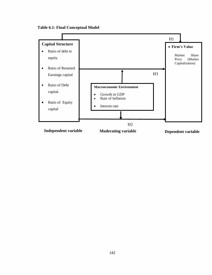
142
Table 6.1: Final Conceptual Model
Dependent variable Moderating variable
H3
H2
H1
Firm’s Value
Market Share
Price (Market
Capitalization)
Capital Structure
Ratio of debt to
equity
Ratio of Retained
Earnings capital
Ratio of Debt
capital.
Ratio of Equity
capital
Macroeconomic Environment
Growth in GDP Rate of Inflation
Interest rate
Independent variable
143
REFERENCES
Abarbanell, J. S. & Bushee, B. L. (1997). Fundamental analysis, future earnings, and stock
prices. Journal of Accounting Research, 35 (1), 1-24.
Abor, J. & Biekpe, N. (2007). How do we explain the capital structure of SMEs in sub-
Saharan Africa? Evidence from Ghana. Journal of Economic Studies, 36 (1), 83-
97.
Adeyemi, B. S. & Oboh, S. C. (2011). Perceived relationship between corporate capital
structure and firm value in Nigeria. International Journal of Business and Social
Science, 19, 131-143
Adongo, J. Strok, C. & Hasheela, E. (2005). Measuring the alternative profit X-efficiency
of Namibia’s Banking Sector. Nepru Research Report, 36(1), 1-58.
Agarawal, R & Zhao, X. (2007). The leverage value relationship puzzle: An industry
effects resolution. Journal of Economics and Business, 59, 286-297.
Aigner, D. K. Lovell & Schmidt, P. (1977). Formulation and estimation of stochastic
frontier production function models. International Economic Review, 17, 377-396
Amit, R. & Shoemaker, P. (1993). Strategic assets and organizational rent. Strategic
Management Journal, 14, 33-46.
Berger, A. N. & Mester, L. J. (1997). Inside the black box: What explains differences in
the efficiencies of financial institutions? The Wharton School, Working Paper
Barney, J. B. (1995). Looking inside for competitive advantage. The Academy of
Management Executive, 9(4), 49-61.
144
Barney, J. B. (2001). Resource-based theory of competitive advantage: a ten-year
retrospective on the resource-based view. Journal of Management, 27(6), 643-650.
Barney, J. B. (1991). Firm resources and sustained competitive advantage. Journal of
Management 17, 771-792.
Baron, R. M. & Kenny, D. A. (1986). The moderator mediator variable distinction in social
psychological research: conceptual, strategic and statistical considerations. Journal
of Personality and Social Psychology, 51(6), 1173-1184.
Battese, G. E. & Coelli, T. J. (1992). Frontier production functions, technical efficiency
and panel data: with application to paddy farmers in India. Journal of Productivity
Analysis, 3: 153-169.
Berger, A. N. & Humphrey, D. B. (1997). Efficiency of financial institutions: international
survey and direction for future research. European Journal of Operational
Research, 98, 175-212.
Berger, A. N. &Mester, L. J. (1997). Inside the black box: what explains differences in the
efficiencies of financial institutions: The Wahrton School, Working Paper.
Booth, L., Aivazia, V., Kunt, A. D. & Makaimovi, V. (2001). Capital structure in
developing countries. Journal of Finance, 87-130.
Brealey, R. & Myers, S. (2008). Pay out policy and cash flow uncertainty. Journal of
Financial Economics, 93(1), 88-107.
Bokpin, G. A. (2009). Macroeconomic Development and Capital Structure Decisions of
Firms. Studies in Economics and Finance, 26(2), 129-142.

145
Brooks, C. (2008). Introductory Econometrics for Finance. New York: Cambridge
University Press.
Callen, J. L. M. & Falk, H. (1993). Agency and efficiency in non-profit organization: the
case of “specific health focus” charities. The Accounting Review, 68(1), 48-65.
Callen, J. L., Morel, M. & Fader, C. (2005). Productivity measurement and the relationship
between plant performance and JIT intensity. Contemporary Research, 159, 239-
249.
Chandler, A. D. (1962). Strategy and structure. Cambridge, MA: MIT Press.
Cheng, Y., Liu, Y. & Tzeng, C. (2011). Capital structure and firm value in china panel
threshold regression analysis. African Journal of Business Management, 4(12),
2500-2507.
Chowdhury, A. & Chowdhury, S. P. (2010). Impact of capital structure on firm value:
Evidence from Bangladesh. Business and Economic Horizons, 3(3), 111–122.
Chung, K. H. & Pruitt, S.W. (1994). A simple Approximation of Tobin’s Q. Financial
Management, 70-74.
Coase, R.W. (1937).The nature of the firm. Economica, 4, 386-405
Cooper R.D. & Schindler P. (2003). Business research methods (8th Ed.). New Delhi: Tata
McGraw-Hill.
146
Cummins, J. D. & Rubio-Misas, M. (2006). Deregulation, Consolidation, and Efficiency:
Evidence from the Spanish Insurance Industry. Journal of Money, Credit, and
Banking, 38(2), 323–355.
Cummins, J. D. & Xie, X. (2008). Market value relevance of frontier efficiency: evidence
from U.S property-liability insurer acquisitions and divestitures, Working paper.
Cummin, W. X. & Zi, (2010). Economies of scope in financial services: A DEA efficiency
Analysis of the US insurance industry. A Journal of Banking and Finance, 38(2),
323-355.
Cummin, W. & Zi, (1999). Organizational Form and Efficiency: The coexistence of stock
and property liability insurers. Management Science, 45(9), 1254-1269.
DeAngelo, H. &Masulis, R. (1980).Optimal capital structure under corporate and personal
taxation. Journal of Finance Economics, 8(1), 3-29.
Demerjian, P., Levy, B. & McVay, S. (2009). Quantifying managerial ability: A new
measure and validity tests. Working Paper, University of Michigan and University
of Utah.
Dess, G. & Beard, D. (1984).Dimensions of organizational task environments.
Administrative Science Quarterly, 29, 52-73.
Dessi, R. & Robertson, D. (2003). Debt, incentive and performance: evidence from UK
panel data. The Economic Journal, 113(490), 903-919.
147
Diacon, S. R., Starkey, K. & O’Brien, C. (2002). Size and efficiency in European long-
term insurance companies: an international comparison. Geneva Papers on Risk
and Insurance 27(3), 444–466.
Dollinger, M. J. (2003).Entrepreneurship. Strategies and Resources, 3rded. Englewood
Cliffs, NJ: Prentice – Hall.
Dopuch, N. & Gupta, M. (1997). Estimation of benchmark performance standards: An
application to public schools expenditures. Journal of Accounting and Economics,
23(2), 141-161.
Dopuch, N., Gupta, M., Simunic, D. A. & Stein, M. T. (2003). Production efficiency and
the pricing of audit services. Contemporary Accounting Research, 20(1), 47-77.
Draniceanu, S. M. (2013). Capital structure and firm value. Empirical evidence from
Romanian listed companies. Journal of Financial Economics, 3(2), 42-53.
Drobetz, W. &Wanzenried, G. (2006). What determines the speed of adjustment to the
target capital structure? Applied Financial Economics, 16(13), 941-958.
Dyer, J. & Singh, H. (1998). The relational view: cooperative strategy and sources of inter-
organizational competitive advantage. Academy of Management Review, 23, 660-
679.
Ebaid, I. E. S. (2012).The impact of capital structure choice on firm performance; empirical
evidence from Egypt. Journal of Risk Finance, 10, 477-487.
Ehrhardt, M. C. & Brigham, E. J. (2003).Corporate finance: A focused approach. 1st ed.
Mason: Thomson.
148
Elsas, R. & Florysiak, D. (2011). Hetegeneity in the speed of adjustment towards the target
leverage. International Review of Finance, 11(2), 181-211
English, M., Grosskopf, S., Hayes, K. & Yaisawarng, S. (1993). Output allocative and
technical efficiency of banks. Journal of Banking and Finance, 17 (2/3), 349-366
Eriotis, N., Vasiliou, D. &Ventoura‐Neokosmidi, Z. (2007). How firm efficiency affect
capital structure: an empirical study. Managerial Finance, 33(5), 321-331.
Fanelli. J. M. & Keifman, S. (2002). Finance and changing patterns in developing
countries, in Fanelli, J. M. and Medhora, R. (Eds), Finance and Competitiveness in
Developing countries.’ London: Routledge.
Fenn, J., Drakos, N. Andrews, W. & Knox, R. E. (2008). Hype cycle for emerging
technologies, Research (Ed, Gartner) Gartner.
Flannery, M. J. &Rangan, K. P. (2006). Partial adjustments towards target capital
structures. Journal of Financial Economics, 79(3), 469-506.
Gachoki, K. M. (2005). Capital structure choice: an empirical testing of pecking order
theory among firms quoted on the Nairobi Security Exchange. Unpublished MBA
project. Nairobi: University of Nairobi.
Galbraith, J. R. (2002). Designing organizations: An executive guide to strategy, structure,
and process. San Francisco; Jossey-Bass.
Ghosh, S. (2007). Leverage, managerial monitoring and firm valuation: a simultaneous
equation approach. Research in Economics, 61, 84-98.
149
Ghoshal, S. & Moran, P. (1996). Bad for practice: A critique of the transaction cost theory.
Academy of Management Review, 21(1), 13–47.
Graham, J. R. & Harvey, C. R. (2001). The theory and practice of corporate finance:
evidence from the field. Journal of Financial Economics, 61(3), 383-416.
Grant, R. M. & Jordan, J. (2012).Foundations of strategy. London: John Wiley & Sons
Ltd.
Grant, R. M. (1991). The resource-based theory of competitive advantage: implications for
strategy formulation. California Management Review, 33(3), 114-135.
Greene, W. L H. & Segal, D. (2004).Profitability and efficiency in the US life insurance
industry. Journal of Productivity Analysis, 21(3), 229-247.
Harvey, C. R., Linsc, K. V. & Roperd, A. H. (2004). The effects of capital structure when
expected agency costs are extreme. Journal of Finance Economics, 74 (1), 3-30.
Holz, C. A. (2002). The impact of the liability-asset ratio and profitability in China’s
industrial state-owned enterprises. China Economic Review, 13, 1-26.
Hurdle, G. (1973). Leverage, risk, market structure and profitability. The Review of
Economics and Statistics, 23, 478-485.
Hutchinson, R. W. (1995). The capital structure and investment decisions of the small
owner-managed firm; some exploratory issues. Small Business Economics, 7, 231-
239.
Inanga, E. L. &Ajayi, C. A. (1999). Accountancy. Lagos: The CIBN Press Limited.
150
Isiki, I. & Hassan, M. K. (2002). Cost and profit efficiency of the Turkish banking industry:
An empirical investigation. The Financial Review, 37(2), 257-280
Jensen, M. & Meckling. W. H. (1976). Theory of the firm: managerial behaviour, agency
costs and ownership structure. Journal of Financial Economics, 3 (2), 305-360.
Johannes, V. W. & Dhanraj, K. (2007). Unlocking shareholder value by moving closer to
the optimal capital structure. Accounting& Tax Periodicals, 28, 171-190.
Johnson, B. & Christensen, L. (2010). Educational research: quantitative, qualitative, and
mixed approaches (2nd edition). Boston, MA: Pearson Education Inc.
Jones, G. R. (2004). Organizational theory, design and change. New Jersey: Addison-
Wesley.
Kadongo, O., Mokoaleli-Mokoteli, T. & Main, L. N. (2014). Capital structure, profitability
and firm value: panel evidence of listed firms in Kenya. Johannesburg: University
of the Witwatersrand.
Kidombo, H. J. (2012). Human resources strategies orientation, organizational
commitment and firm performance in large private manufacturing firms in Kenya.
Unpublished PhD thesis. Nairobi: University of Nairobi.
Kinuu, D. (2014). Top management team psychological efficiency, institutional
environment, team processes and performance of companies listed in Nairobi
securities exchange. Unpublished PhD thesis. Nairobi: University of Nairobi.
Kiogora, (2000). Investigation of the existence of optimal capital structure decisions
among industry firms. Unpublished MBA project. Nairobi: University of Nairobi.

151
Kohher, R. (2007). Strategic assets, capital structure, and firm performance. Journal of
Financial and Strategic Decisions, (3), 23-26.
Korajczyk, R. A. & Levy, A. (2003). Capital structure choice: Macro-economic conditions
and financial constraints. Journal of Financial Economics, 68, 75-109.
Kothari, C. R. (2004). Research methodology, methods and techniques, 2nded. New Delhi:
New Age International (P) Ltd.
Kumbhakar, S. S. Ghosh & McGuckin, J. (1991). A generalized production frontier
approach for estimating determinants of inefficiency in US dairy farm. Journal of
Business and Economic Statistics, 9, 279-286.
Krishnaswamy, C.R., Mangla, I. &Rathinasamy, R.S. (1992). An empirical analysis of the
relationship between financial structure and market structure. Journal of Financial
and Strategic Decisions, 5(3), 75-88.
Letangule, S. L. & Letting, N. K. (2012). Technological Innovation and Corporate
Performance. IJMBS, 2(3), 66-72.
Linh, N. H. (2014). How firm efficiency affect capital structure. An analysis of Finnish
technology industry. Unpublished Ph.D. Thesis Lahti University of Applied
Sciences.
Madhok, A. (2002). Reassessing the fundamentals and beyond: Ronald Coase, the
transaction cost and resource-based theories of the firm and the institutional
structure of production. Strategic Management Journal, 23(6), 535–550.
152
Magutu, O. P. (2013). Supply chain strategies, technology, and performance of large- scale
manufacturing firms in Kenya. Unpublished PhD thesis. Nairobi: University of
Nairobi.
Majumdar, S. K. & Chhibber, P. (1999). Capital structure and performance: evidence from
a transition economy on an aspect of corporate governance. Public Choice, 98, 287-
305.
Malhatra, P. & Singh, B. (2009). The impact of internet banking on bank performance and
risk: the Indian experience. Eurasian Journal of Business and Economics, 2(4), 43-
62.
Maudos, J. & Pastor, J. M. (2003). Cost and profit efficiency in the Spanish banking sector
(1985-1996): a non-parametric approach. Applied Financial Economics, 13, 1-12.
McConnel, J. J. & Servaes, H. (1995). Equity ownership and the two faces of debt. Journal
of Financial Economics, 39, 131-157.
Mensah, Y. M. & Li, S. H. (1993). Measuring production efficiency in a not –for-profit
setting: an extension. The Accounting Review, 68 (1), 66-88.
Miguel, A. & Peinado, C. (2004). Optimal capital structure, endogenous bankruptcy, and
the term structure of credits spreads. Journal of Finance, 51(3), 987-1019.
Modigliani, F. & Miller, M. H. (1958). The cost of capital, corporate finance and the theory
of investment. American Economic Review, 48, 261-297.
Modigliani, F. & Miller, M. H. (1963). Corporate income taxes and the cost of capital: a
correction. American Economic Review, 53(3), 433-443.

153
Mugenda, O. M. & Mugenda, A. G. (2003). Research methods: Quantitative and
qualitative approaches. Nairobi: Acts Press.
Muia, J. M. (1997). The nature and determinants of the wealth portfolios of salaried middle
and upper income employees in Kenya. Unpublished PhD thesis. Nairobi:
University of Nairobi.
Murgor, P. K. (2014). External environment, firm capabilities, strategic responses and
performance of large scale manufacturing firms in Kenya. Unpublished PhD thesis.
Nairobi: University of Nairobi.
Mwangi, L. W., Makau, M. S. & Kosimbei, G. (2014). Relationship between capital
structure and performance of non-financial companies listed in the Nairobi
securities exchange. Global Journal of Contemporary Research in Accounting,
Auditing and Business Ethics, 1(2), 72-90.
Myers. S. C. &Majluf, N. (1984). Capital financing and investment decisions when firms
have information investors do not have. Journal of Financial Economics, 13,187-
221.
Nairobi securities exchange handbook (2014).
Ngugi, R. & Njiru, R. (2005). Growth of Nairobi Stock Exchange primary market. KIPPRA
discussion paper No .47. Nairobi: KIPPRA.
Ongeti, W. J. (2014). Organization resources, corporate governance structures and
performance of Kenyan state corporations. Unpublished Ph.D thesis. Nairobi:
University of Nairobi.
154
Ozkan, A. (2001). Determinants of capital structure and adjustment to long run target:
evidence from UK company panel data. Journal of Business Finance & Accounting,
28(1-2), 175–198.
Pandey, I. M. (1999). Financial management (8th ed.). New Delhi: Vikas Publishing
House PVT Ltd.
Parrino, R. & Weisbach, M. S. (1999). Measuring investment distortions arising from
stockholder-bondholder conflicts. Journal of Financial Economics, 3-42.
Pasanen, M. (2003). In search of factors affecting SME performance: the case of Eastern
Finland. Unpublished Ph.D Thesis. Kuopio: University of Kuopio.
Pearce, J. A., Robinson, R. B. & Mital, A. (2012). Strategic management: formulation,
implementation and control, 12th edition. New Delhi: Tata McGraw Hill Education
Private Ltd.
Penrose, E. (1959). The theory of growth of the firm. New York: Wiley & Sons.
Peteraf, M. A. (1993). The cornerstones of competitive advantage: A resource-based view.
Strategic Management Theory, 14(3), 179-191.
Pfeffer, J. & Salancik, G. R. (1978). The external control of organizations: a resource
dependence perspective. New York: Harper & Row.
Porter, M. E. (1985). Competitive advantage: Creating and sustaining superior
performance. New York: Free Press.

155
Porter, M. E. & Linde van der, C. (1995).Green and competitive: Ending the stalemate.
Harvard Business Review, 21, 119-134.
Priem, R. L. & Butler, J. E. (2001). Is this resource based ‘view’ a useful perspective for
strategic management research? Academy of Management Review. 26(1), 22-40.
Priem, R. L., & Butler, J. E. (2001). Is the resource-based theory a useful perspective for
strategic management research? Academy of Management Review, 26, (1), 22–40.
Rao, N. V., Al-Yahyee, K. & Syed, L. (2007). Capital structure and financial performance:
evidence from Oman. Indian Journal of Economics and Business, 1-23.
Rathinasamy, R. S., Krishnaswamy, C. R. & Mantripragada, K. G. (2002). Capital structure
and product market interaction: An international perspective. Global Business and
Finance Review, 5(2), 51-63.
Rayan, K. (2008). Financial leverage and firm value. Gordon Institute of Business Science,
University of Pretoria.
Robson, C. (2011). Real world research: a resource for users of social research methods
in applied settings. 3rd ed. Chichester: Wiley.
Rouse, P., Putteril, M. & Ryan, D. (2002). Integrated performance measurement design:
Insight from an application in aircraft maintenance. Management Accounting
Research, 13(2), 229-248.
Saunders, M., Lewis, P. & Thornbill, H. A. (2007). Research methods for business
students.4th Ed. Harlow: Prentice Hall, Pearson Education Limited.
156
Sekaran, U. (1992). Research methods for business: A skill building approach, 2nded. John
Wiley & Sons, Inc
Schall, L. D. (1984). Taxes, inflation and corporate financial policy. The Journal of
Finance, 39 (1), 105-126.
Scholtens, B. & Wensveen, D. (2002). The theory of financial intermediation: an easy on
what it does (not) explain. SUERF, Vienna.
Scott, D. F. Jr. &Martin, J. D. (1976). Industry influence on financial structure. Financial
Management, 6, 35-42.
Simerly, R. & Li, M. (2000).Environmental dynamism, financial leverage and
performance; a theoretical integration and an empirical test. Strategic Management
Journal, 21, 31-49.
Soliman, M. T. (2008). The use of DuPont analysis by market participants. The Accounting
Review, 83(3), 823-853.
Song Shin, H., & Adrian, T. (2009). Federal Reserve Bank of New York
staffReports.http:papers.ssrn.com/.
Stone-Romero, E. F. & Liakhovitski, D. (2002). Strategies for detecting moderator
variables: A review of conceptual and empirical issues. Research in Personnel
and Human Resources Management, 21, 333-372.
Tajala, A. (2012). Testing VRIN framework: resources value and rareness as sources of
competitive advantage and above average performance. Management, 17 (2), 51-
64.
157
Tan, J. J. &Litsschert, R. J. (1994). Environment-strategy relationship and its performance
implications: An empirical study of the Chinese electronics industry. Strategic
Management Journal, 15(1), 23-34.
Weill, L. (2008). Leverage and corporate performance: Does institutional environment
matter? Small Business Economics, 30, 251–265.
Weiss, D. (2010). Cost behaviour and analysts earnings forecast. The Accounting Review,
85(4), 1441-1471.
Wernerfelt, B. (1984). A resource based view of the firm. Strategic Management Journal,
5,171-180.
Wiklund, J. & Shepherd, D. (2003). Knowledge-based resources, entrepreneurial
orientation, and the performance of small and medium-sized businesses. Strategic
Management Journal, 24, 1307–14.
Williamson, O. E. (1998). The mechanisms of governance. New York: Free Press.
Williamson, O. E. (1985). The economics institutions of capitalism: firms, markets,
relational contracting. New York: The Free Press.
Woodward, J. (1958). Contingency school of management. Retrieved on 14/09/2012 from
http/victorstudy.com/management schools/contingency school.
World Bank /KIPPRA, RPED Kenya, 2003.
158
Worthington, A. C. (2009). Frontier efficiency measurement in deposit-taking financial
mutual: a review of techniques, application and future research directions. Griffith
Business School, Discussion Papers Finance, (11).
Worthington, A. C. (2004). Determinants of merger and acquisition activity in Australia
co-operation deposit-taking institutions. Journal of Business Research, 57(1), 47-
57.
Zikmund, W. G., Babin, B. J., Carr, J. C. & Griffin, M. (2010). Business Research Methods,
8th Edition. South-Western, Cangage Learning.
Zhao, B. & Wijewardana, W. P. (2012). Financial leverage, Firm growth and financial
strength; Evidence in Sri Lanka. Journal of Asian Pacific Business Innovation and
Technology Management, 2, 14-22.

159
APPENDICES
Appendix I: Introduction Letter

160
Appendix II: Data Collection Form
Company-------------------------------------------------------------------------------
Date of incorporation-----------------------------------------------------------------
QUESTIONS VARIABLE Source: Financial
Statements
(Records
Maintained at NSE)
and CBK Data
2009 2010 2011 2012 2013 2014
1 FIRM SPECIFIC efficiency
i Turnover Income statement
OPERATIONAL AND COST EFFICIENCY
1 Administrative costs Income statement
2 Distribution costs Income statement
3 Financing cost Income statement
4 Taxation cost Income statement
5 Total Operational
Costs
Income statement
B PROFIT EFFICIENCY
1 Profit before tax
(EBIT)to be
computed using
SFA)
Income statement
2 Interest Costs(To be
computed using
SFA)
Income statement
3 Taxation Costs(To
be computed using
SFA)
Income statement

161
4 Profit after tax (To
be computed by
SFA)
Income statement
5 Amount of Retained
Earnings(To be
computed using
SFA)
Income statement
2 CAPITAL STRUCTURE
A Amount in KSHS of
Retained Earnings
Balance Sheet
B Amount in KSHS of
debt capital
C Amount in KSHS of
Equity capital
Balance Sheet
3 MACRO ECONOMIC ENVIRONMENT
A Interest rate KNBS and Central
Bank of Kenya (Hand
book/website)
B Growth in GDP KNBS and Central
Bank of Kenya (Hand
book/website)
C Inflation KNBS and Central
Bank of Kenya (Hand
book/website)
4 FIRM VALUE
A No of Equity shares Balance sheet
162
B Earnings per share Income
Statement/Balance
sheet
C Share market price Market information
section, balance
sheet/statement of
financial position,
financial ratios
D Market
capitalization(Market
price per share
multiplied by
outstanding equity
shares)
Market information
section, balance
sheet/statement of
financial position,
financial ratios

163
Appendix III: Listed Companies at NSE
1. A Baumann &Co.
2. ARM Cement
3. Bamburi Cement
4. BOC Kenya Ltd
5. British American Tobacco Kenya Ltd.
6. Car and General
7. Carbacid Investments Ltd
8. CMC Holdings
9. Crown Paints Kenya
10. E.A Cables
11. E.A Portland
12. E.A. Breweries Ltd.
13. Eaagadds
14. Elliots
15. Eveready East Africa Ltd.
16. Express Ltd.
17. Hutchings Biemer Ltd.
18. Kakuzi Ltd.
19. Kapchorua Tea.
20. Kengen
21. Kenolkobil
22. Kensalt
23. Kenya Airways Ltd.
24. Kenya Orchards Ltd.
25. KP&LC
164
26. Limuru Tea.
27. Longhorn Kenya
28. Marshalls (E.A)
29. Mumias Sugar Company Ltd.
30. Nation Media Group Ltd.
31. Rea Vipingo Ltd.
32. Safaricom ltd
33. Sameer Africa
34. Sasini Tea Ltd.
35. Scan Group Ltd.
36. Standard Group Ltd.
37. Total Kenya
38. TPS (Serena) Ltd.
39. Uchumi Supermarkets Ltd.
40. Umeme Ltd.
41. Unga Group Ltd.
42. Williamson Tea.
Source: Nairobi Securities Exchange: Hand book 2014

165
Apendix IV: Authorization Letter from NACOSTI

166
Appendix V: Research Clearance Permit from NACOSTI