Financial Vulnerabilities, Macroeconomic Dynamics,and Monetary Policy∗

David Aikman† Andreas Lehnert‡ Nellie Liang§ Michele Modugno¶

April 12, 2016

Abstract

We define a measure to be a financial vulnerability if, in a VAR framework that al-lows for nonlinearities, an impulse to the measure leads to an economic contraction. Weevaluate alternative macrofinancial imbalances as vulnerabilities: nonfinancial sectorcredit, risk appetite of financial market participants, and the leverage and short-termfunding of financial firms. We find that nonfinancial credit is a vulnerability; a highcredit-to-GDP gap leaves the economy less resilient to adverse events. Monetary pol-icy is generally ineffective at slowing the economy once the credit-to-GDP gap is high,suggesting potential benefits from avoiding excessive credit growth. Impulses to riskappetite lead to an economic expansion, though also to a higher credit gap over thelonger-term. We also find that financial sector “runnable” liabilities are a vulnerabil-ity, consistent with the fragility of short-term funding and importance for transactions,though financial sector leverage relative to its trend appears to reflect investor riskappetite.

Keywords : Financial stability and risk, monetary policy, credit

JEL classification: E58, E65, G28

∗We would like to thank Maria Perozek, Shane Sherlund, and Cindy for help and advice in constructingsome of the measures we use. We benefitted from helpful comments from Tobias Adrian, William Bassett,Rochelle Edge, Oscar Jord and Michael Kiley. Luc Laeven and Richard Berner provided helpful commentsas discussants at the Federal Reserve Bank of Boston’s conference “Macroprudential Monetary Policy”, heldon Oct. 2-3, 2015. Collin Harkrader provided excellent research assistance. Any remaining errors are ownresponsibility. The views expressed here are ours and not those of our employers.†Bank of England, David.Aikman@bankofengland.co.uk‡Board of Governors of the Federal Reserve System, andreas.lehnert@frb.gov§Board of Governors of the Federal Reserve System, jnellie.liang@frb.gov¶Board of Governors of the Federal Reserve System, michele.modugno@frb.gov

1

1 Introduction

The recent global financial crisis highlighted in dramatic fashion the damage to economicperformance from falling asset prices amid high levels of credit and fragile financial insti-tutions. Policymakers have since been encouraged to monitor the financial system for thebuildup of so-called macrofinancial “imbalances” that could make the system vulnerable toshocks such as a large decline in asset prices. Indeed, cross-sectional studies of advancedeconomies have found that private nonfinancial sector credit and asset valuations are earlywarning indicators of economic recessions and financial crises (see Borio and Lowe (2002),Drehmann and Juselius (2015), Schularick and Taylor (2012)). In addition, studies havefound that high credit growth and asset bubbles combined lead to significantly weaker eco-nomic recoveries (see Jorda et al. (2013)). Financial stability monitoring frameworks, basedon this growing body of theoretical and empirical research, focus on the levels and growthrates of these macrofinancial imbalances as potential vulnerabilities of the financial system(see Adrian et al. (2013)).

In this paper, we systemically evaluate several commonly-cited macrofinancial imbalancesfor whether they lead to higher risks to future macroeconomic performance. We shed em-pirical light on this question using a threshold VAR model using data for the U.S. economyfrom 1975 to 2014. Using alternative measures of macrofinancial imbalances, we test whethershocks to the measures lead to subpar economic performance, specifically lower GDP anda higher unemployment rate. We test for nonlinear dynamics by dividing the sample intoperiods depending on whether the measure is above or below its average. Measures of finan-cial imbalances that are found to lead to weaker expected economic performance are definedto be “vulnerabilities.” (Henceforth, we use the term vulnerability to refer generically tovariables that measure candidate macrofinancial imbalances that might lead to economiccontractions.)

We examine four vulnerabilities often cited in studies of financial crises: private-sectordebt, investor sentiment or asset valuations, financial-sector leverage and maturity transfor-mation among financial institutions.1 We briefly describe each candidate vulnerability inturn, how we measure it, and the rationale for including it in our framework.

Note that the first two of our candidate vulnerabilities, debt and asset valuations, areconceptually different from financial-sector leverage and maturity transformation. The firstset are economy-wide measures and do not depend on particular institutional features. Thesecond are defined relative to specific financial institutions such as money market mutualfunds or banks.

The first measure is private-sector debt, using primarily the credit-to-GDP gap, defined asthe difference between the ratio of private nonfinancial sector credit outstanding to GDP andits long-term trend (e.g.Borio and Lowe (2002, 2004); Borio and Drehmann (2009)).2 We alsoevaluate alternative disaggregations of this measure–household vs. business borrowers, bank

1We do not consider the current-account balance as a potential vulnerability in our framework. Whilethis has been emphasized in cross-country studies of small open economies, we leave this as a future exercisein our framework.

2Borio and Lowe (2002) evaluate the roles of rapid credit growth and rising asset prices as amplifiers, andfind in cross-section analysis that the private nonfinancial credit-to-GDP gap is a high-quality early-warningindicator of recessions, and also is useful when combined with property prices.

2

vs. nonbank credit, debt collateralized by property vs. other debt-to test more hypothesesabout specific vulnerabilities, such as the role of real estate, which is often identified as akey risk to financial stability.

A second measure is the extent of “froth” in financial markets – that is, relatively richasset valuations or relatively high investor risk appetite. We construct a direct measure ofinvestor risk appetite, dubbed ALLM, based on asset valuations and lending standards infour markets: business credit, commercial real estate, household credit (including consumercredit and residential mortgages), and equities. We also consider the excess bond premiumof Gilchrist and Zakrajek (2012) as a measure of risk appetite, which has been found to bea useful predictor of macro performance. Higher asset values relative to historical averagesmay reflect greater risk-taking behavior which could lead to a buildup in financial vulnera-bilities and make the economy less resilient to to adverse shocks. Boom-bust cycles in realestate prices are viewed by many economists as key sources of financial fragility (see, forinstance, Cecchetti (2008), Iacoviello (2005), and Jorda et al. (2015)). Others have empha-sized the information in bond risk premiums (Stein (2013b) and Lopez-Salido et al. (2015)).According to this view, when risk premiums are unusually low there is a greater probabilityof a subsequent rapid reversal, which may be associated with significant adverse economic ef-fects. Brunnermeier and Sannikov (2014), among others have argued that low volatility mayspur risk taking, with the potential for a destabilizing unraveling when volatility eventuallyspikes.

Our third measure is the leverage of the financial sector. This is an obvious potential vul-nerability because more-leveraged financial institutions are less able to absorb losses. Facedwith solvency concerns, these intermediaries may need to shrink, with negative consequencesfor the broader economy from fire sales or reduced credit supply. Of course, the leverageof financial intermediaries cannot rise in the absence of investor willingness to finance theirborrowing, suggesting that risk appetite may play some role in leverage, a dynamic high-lighted by Geanakoplos (2010). Further, Adrian and Shin (2010, 2014) document that theleverage employed by a crucial class of financial institution–broker dealers–is highly procycli-cal, in line with the tendency of asset price volatility to be low in booms and high in busts.We construct an aggregate measure of total assets to equity for financial intermediaries thatare leveraged, including depository institutions, insurance companies, broker dealers, financecompanies, REITs, and holding companies from the Financial Accounts of the U.S.

Our last measure is related to maturity transformation of financial institutions. Thisfunction and its role as an amplification mechanism have been studied by Adrian and Bo-yarchenko (2015) and Gertler and Kiyotaki (2015), among others. We approximate maturitytransformation by financial intermediaries with non-deposit claims that are pay-on-demandbut that carry credit risk, based on Bao et al. (2015). Our measure comprises five com-ponents which have data back to 1975: repurchase agreements (repo), securities lending,retail and institutional money market mutual funds (MMMFs), and commercial paper. Thegreater the prevalence of these “runnables”, the greater the exposure of the economy toa self-fulfilling withdrawal by investors which in turn precipitates a series of fire sales anddeleveraging by financial intermediaries. In principle, the importance of this channel hasbeen recognized since Diamond and Dybvig (1983). More recently, wholesale liabilities ofthe banking sector have been found to be an indicator of banking crises in cross-sectionalstudies (Anundsen et al. (2014)), and short-term liabilities in the repo market and asset-

3

backed commercial paper market were subject to runs in the U.S. financial crisis (Gortonand Metrick (2012) and Covitz et al. (2013)). Krishnamurthy and Vissing-Jorgensen (2015)argue that issuance of Treasury debt affects the supply of short-term liquid claims issued byfinancial institutions, which are associated with financial crises.

Our tests indicate that private-sector debt is indeed a vulnerability in the sense of pre-saging economic contractions, while shocks to risk appetite are expansionary. Specifically,a primary finding is that impulses to the credit-to-GDP gap lead to decreased output andhigher unemployment when the credit gap is above zero, indicating that the credit gap is avulnerability. These results suggest that when the economy has a high credit gap, it is morevulnerable to adverse events which lead to recessions. By contrast, in the early phase of thefinancial cycle when the credit gap is low, credit shocks do not have adverse effects; indeed,they stimulate economic growth, consistent with the equilibrium relationship between debtand economic growth more common to macroeconomic models. Another primary findingis that the responses to monetary policy impulses also suggest nonlinearities that dependon the level of the credit gap. When the credit gap is low, impulses to monetary policylead to an increase in unemployment, a contraction in GDP, and a decline in credit, all asexpected. However, when the credit gap is high, output, unemployment, and credit appearunresponsive to similar impulses to monetary policy.

Our finding that monetary policy shocks have less effect on activity and inflation whendebt-to-GDP is above trend is consistent with at least two theories. First, as asset priceincreases and associated credit growth gain steam, monetary policy may be less effectiveat restraining activity (see Dokko et al. (2009)), perhaps because an overriding speculativemotive made increases in the cost of funds a relatively less important consideration. (Footeet al. (2012); Cheng et al. (2014)). Second, monetary policy may be less effective at stimu-lating activity after a credit-fueled boom, perhaps because the overhang of debt accumulatedduring the boom reduces consumers’ or firms’ capacity to borrow (Guerrieri and Lorenzoni(2015); Dobridge (2016)) or because the boom stimulated a misallocation of resources (Mianet al. (2015)). We shed some light on this by redefining our threshold in terms of the growthof the debt-to-GDP ratio, so that the sample is divided in periods when the ratio is rising orfailing rather than high or low. We find that monetary policy is ineffective when the ratiois rising but effective when it is falling, suggesting perhaps more support for the first storyrather than the second.

Turning to investor risk appetite, we find that impulses to our measure, ALLM, arefollowed by economic expansions in the near term. Thus, it does not meet our definitionof a vulnerability. This result is not surprising: when financial conditions become moreaccommodative, economic performance improves. However, this positive effect is smallerwhen ALLM is already high.

An obvious channel by which risk appetite could affect economic performance is via creditgrowth. Indeed, we find that a shock to ALLM does stimulate an increase in the credit-to-GDP gap. Moreover, the effects of a shock to ALLM on the credit gap tend to be largerin periods when the credit-to-GDP gap is already high. There is some suggestion that, leftlong enough, this dynamic could push the credit-to-GDP gap sufficiently high to produce aneconomic contraction.

Taken together, the results for impulses to credit and ALLM suggest the following story:exogenous increases in credit lead to a misallocation of resources or leave agents more exposed

4

to inevitable negative shocks. Moreover, during episodes of high credit-to-GDP, agents’willingness to borrow and lend is less sensitive to the cost of funds. What might spark sucha rise in credit relative to income? An increase in ALLM is one clear possibility suggestedby our results.

Turning to the other candidate vulnerabilities, we find that financial sector leverage hassimilar dynamics in the near term to the ALLM measure in that shocks are expansionary.Thus, it does not satisfy our definition of a vulnerability. We also find that shocks to therunnable liabilities-to-GDP gap result in economic contractions when the gap is high butnot when it is low; thus, the runnables gap, like the credit gap, does meet our definition ofa vulnerability.

There are a few explanations for this pattern. The work of Adrian and Shin (2010)suggests a strong linkage between financial leverage and asset prices and volatility, and thus,potentially, risk appetite, but not necessarily to real economic activity. A decline in runnablesappears associated with a decline in economic activity, which makes obvious intuitive sensebecause of the strong tie of short-term funds to transactions. A decline in leverage, however,could be driven either by mounting losses, as following a peak in the credit cycle, or byincreased risk aversion, as in periods of low risk appetite and tight financial conditions. Itmay also be the case that, because of the growth of the derivatives market, leverage hasbecome more difficult to measure.

We conduct a number of robustness tests, particularly in cases where the variable weuse may only imperfectly measure the underlying vulnerability. For example, as discussedearlier, we use a number of different proxies for the level of asset valuations or investorrisk appetite. In addition, we consider alternatives to the credit-to-GDP gap, including aspecification with just the (log) level of credit and replacing actual GDP with potential GDP.

Our results bear on several strands of the literature. We show that a number of macrofi-nancial aggregate measures have implications for real activity and employment in the U.S.,adding to the empirical literature on the role of financial variables in business cycles, startingwith Bernanke and Gertler (1989). Our results indicate that a high credit gap makes theeconomy less resilient and increases the likelihood of a recession. These findings suggestsome important financial frictions that affect macroeconomic performance, such as borrow-ing being driven by changes in the supply of credit (see Lopez-Salido et al. (2015) and Mianet al. (2015)), or that individuals do not consider the effects on aggregate credit when theymake their borrowing decisions (as suggested in a model by Korinek and Simsek (2014)). Inaddition, while others have identified a role for shocks to certain credit aggregates and assetprices to contribute to business cycle fluctuations, this paper is the first to systematicallyexamine a commonly-cited set of financial vulnerabilities, including those specific to the fi-nancial sector. In particular, impulses to short-term wholesale liabilities of financial firmsincrease the likelihood of subpar economic activity, perhaps because they leave the systemvulnerable to fire sales and significant disruptions in transactions.

Second, our finding that macroeconomic responses are nonlinear and depend on whetherthe credit gap is above or below normal adds to a growing line of research arguing thattransmission channels may operate differently depending on underlying conditions. Hubrichand Tetlow (2012) use a regime switching model to evaluate the relative effectiveness ofmonetary policy by whether the economy is in a financial crisis state. Meitu, Hilberg, andGrill (2014), find a strong asymmetry in the macroeconomic responses to a risk premium

5

shock depending on whether credit conditions are normal or tight.Finally, our finding that monetary policy is less effective when the credit gap is high,

combined with our finding that a high credit gap is a vulnerability, suggests that creditis costly and may lead to more severe recessions. For example, Jorda et al. (2013) provideevidence that excess credit creation in the period preceding a recession substantially increasesthe depth of the subsequent recession, for both normal recessions and financial recessions(those with substantial losses to the banking sector).3

The relative ineffectiveness of monetary policy also is relevant for evaluating the use ofmonetary policy to reduce vulnerabilities and future crises, relative to the use of macropru-dential policies. Svensson (2015) argues that the costs of directing interest rates at financialstability risks (in terms of reduced output today) would almost always significantly exceedthe benefits (reduced probability of a future crisis by reducing credit growth). Ajello et al.(2015) look at whether monetary policy should respond to the risk of a financial crisis whichdepends on credit conditions (lagged bank loan growth), based on a calibrated model of theU.S. economy. They find that optimal interest rate policy does respond to crisis risk, butonly by a very small amount. Our results provide stronger support for the use of monetarypolicy: credit is a vulnerability and a high credit gap leaves the economy less resilient andmore prone to a recession. If monetary policy is increased and reduces the amount of credit,it not only would reduce the probability of a crisis but also the severity of a subsequent re-cession. Given monetary policy is not effective in a high credit gap state, there may be highreturns to policymakers from avoiding such states. More targeted macroprudential policiesmay be a preferable way to reduce credit, but a high share of market-based finance maylead to situations in which such macroprudential measures’ effectiveness is diminished andmonetary policy should be considered.

The remainder of our paper is organized as follows: in section 2 we describe and charac-terize our proxies for vulnerability; in section 3 we evaluate whether credit and risk appetite,separately and jointly, satisfy our definitions of a macrofinancial vulnerability. In section 4 weevaluate whether the measures tied to the leverage and maturity transformation of financialinstitutions, satisfy our definition. Section 5 concludes.

2 Data and Specification

In this section we describe the candidate measures of vulnerabilities that we test and thespecification that we use to test them. In terms of the series, in certain cases importantstructural changes in the financial environment – including changes to the U.S. bankruptcycode – will motivate the use of certain subperiods of our sample. Our outcomes of interestare subpar economic performance – contractions in GDP and increases in the unemployment

3For example, in the fourth year after the peak, in a normal recession, the economy is well into a recovery,with real GDP per capita estimated to be 3.8 percentage points higher than the cyclical peak. But hadcredit exceeded average levels by one standard deviation, real GDP per capital would be estimated to be1.8 percentage points less, at 2.0 percent. In the case of a financial recession, the effects are larger. In thefourth year after the peak, the economy has still not recovered, the GDP per capita level is -2.8 percentagepoints below the cyclical peak for average excess credit. If credit were one standard deviation higher, realGDP per capita would be as low as 3 percentage points lower, at -5.8 percent. These suggest significanteffects for excess credit on the severity of the subsequent recession.

6

rate – rather than full-blown financial crises. This is because there are relatively few financialcrises in the U.S. data since 1975. Of the four U.S. recessions in that period, only the 2007 to2009 episode has been defined to be a financial crisis (in Reinhart and Rogoff (2009)). Thewave of bank failures that began in 1984 and culminated in 1988-1992 with the failure ofalmost 1,600 depository institutions associations has also been labelled a crisis (see Laevenand Valencia (2008)), suggesting that perhaps the 1990 recession could also be associatedwith a financial crisis. Jorda et al. (2013) find that roughly 30 percent of recessions in theirsample of 14 advanced economies from 1870 to 2008 involve financial crises.

2.1 The credit-to-GDP gap

We follow the literature in defining the credit-to-GDP gap as the difference between the ratioof nonfinancial private sector debt to GDP and an estimate of its trend, which is designedto be slow-moving. In addition to testing this broad measure, we also test the componentsin three separate decompositions of the credit-to-GDP gap:

1. A sectoral decomposition of credit provided to households vs. to businesses;.

2. A collateral decomposition of credit backed by property (commercial or residential)vs. other forms of credit; that is, unsecured credit or credit secured by non-propertycollateral.

3. A bank vs. nonbank decomposition, based on where the credit exposures are beingheld.

As shown in figure 1, the credit-to-GDP ratio since 1975 shows two distinct build-ups:the first starts in the early 1980s and ends in the recession of 1990-91; the second starts inthe late 1990s and accelerates for a sustained period until the Great Recession. Even afterfalling significantly from its peak in 2009, the level remains elevated relative to previousdecades.

The estimated gap, the ratio less a trend estimated with a HP filter with a smoothingparameter of 400,000, shows a similar pattern over history, with peaks ahead of the recessionsof 1990-91 and 2007-9. The gap we report is based on final estimates of credit-to-GDP; real-time estimates provided an earlier warning and showed the sustained increase starting earlier,during the mid-1990s (see Edge and Meisenzahl (2011) for a discussion of real-time vs finalestimates of the credit-to-GDP gap.)

The figure highlights a well-known property of the credit-to-GDP gap: that it tends behigh for a significant period after the financial cycle turns, which may have implications forthe strength of a recovery. The gap also tends to continue to increase during the recessionbefore turning down, which may reflect borrowers drawing upon pre-committed lines of creditthat they have with banks in such situations, which delays the recognition of tight financingconditions in credit measures, or that GDP, the denominator of the ratio, may fall morequickly than credit in the early stages of a downturn because of long-lived debt contracts,such as mortgages. In our empirical analysis we consider some alternative measures includingthe level of credit and the credit gap estimated using potential GDP. This latter measurein particular removes the mechanical increase in the ratio (and hence the gap) caused by adecline in GDP.

7

Another concern with using measures based on credit-to-GDP is the upward trend inthe ratio. As an empirical matter, this is dealt with by focusing on the gap with respectto an estimate of the trend designed to be slow moving. As a theoretical matter, the trendis often ascribed to financial deepening, as credit markets have evolved to make loans moreaccessible to previously unserved households and businesses.

Decomposing the credit-to-GDP ratio into its components shows that the upward trendin the U.S. is largely due to an increase in household credit. As shown in the middle panelof figure 1, household credit has nearly doubled since 1975, while the increase in businesscredit has been more modest. Household credit rose both because of the extensive margin– more households became homeowners – and the intensive margin – existing homeownerstook on more debt. These increases are due to a combination of public policies, including thetax advantage of mortgage debt and the funding advantage enjoyed by the housing-relatedgovernment-sponsored enterprises, Fannie Mae and Freddie Mac.4 On the extensive margin,the homeownership rate also rose: from 64.0 in 1990:Q1 to a peak of 69.2 in 2004:Q4 (sincethen it has fallen steadily, returning to its 1990 level).

Household and business credit-to-GDP gaps (middle panel of figure 1) clearly illustratethe lower frequency of cycles in the household credit gap relative to the business credit gap,as well as the differences in amplitude of changes. Differences in the household and businesscredit gaps may be important for setting macroprudential policies if one of the sectors provesto be a more prominent vulnerability than the other, and we evaluate this proposition inestimations below.

The bottom panels of figure 1 decompose the credit-to-GDP ratio into credit providedby banks and nonbanks. Our measure of nonbank credit gathers many different types ofproviders, including: shadow banks, which offer credit which is funded by short-term debtwithout insurance or a public backstop; the GSEs; pension funds and life insurers, which tendto have long-dated liabilities; and mutual funds, which issue shares that are loss-absorbing(see Bassett et al. (2015) for more detail).

The bank credit-to-GDP ratio appears to be stationary, and has gone through threecycles, roughly in sync with household credit, with peaks in the late 1970s, late 1980s, andthen in 2009.

The nonbank credit-to-GDP ratio shows a secular upward trend, due importantly to thegrowth of shadow banks and the GSEs, though it too fell sharply in 2008, when shadow bank-ing collapsed. Rajan (2005) argues that developments in financial markets – deregulation,technological and financial innovations, and globalization–have lowered financial frictionsand improved efficiency, but may also lead to new and higher risks. For example, credit thatis increasingly funded via financial markets rather than bank deposits makes credit moresensitive to market disturbances.

4The share of mortgage credit funded by Fannie and Freddie grew from 12 percent in 1975 to roughly60 percent in 2014. (Financial Accounts of the United States, table L.218.) The GSEs faced lower capitalcharges for funding residential mortgages than did banks, and benefited as well from an implicit backstopby the U.S. government. For a discussion of the capital advantages enjoyed by the GSEs, see Hancocket al. (2006). A large pre-crisis literature debated the extent to which the GSEs lowered borrowing costsfor homeowners. This debate centered in large part on the role of the GSEs’ retained portfolios; that is, theGSEs’ practice of buying the very securities they issued. See Passmore (2005).

8

2.2 Measures of risk appetite

Our second candidate measure is an index related to investors’ willingness to accept risk thatwe constructed (denoted ALLM). To link the existing literature we compare our measure tothe excess bond premium measure (EBP) of Gilchrist and Zakrajek (2012). Both measures(the top panel of figure 2) are more volatile than the credit-to-GDP ratio and show morecycles.

We construct our measure, ALLM, in the spirit of the methodology described in Aikmanet al. (2015). The measure includes indicators of asset price valuations and lending stan-dards in four areas: equity markets; business credit; commercial real estate; and householdand residential mortgage credit. The overall measure is then a weighted average of the stan-dardized index for each of the four sectors.5 The bottom panel of figure 2 shows the fourcomponents.

The equity and business credit components of ALLM are quite similar to the EBP, al-though ALLM recovers somewhat more slowly after the 1990 and 2008-09 recessions becauseit also includes credit conditions for small businesses, whereas the EBP is based on onlypublicly-traded corporations. However, ALLM also reflects changes in commercial and res-idential mortgage credit availability; these markets have cycles distinct from asset markets.As a result, the overall ALLM index is distinctly below the (negative) EBP in the late 1970s,when equity markets fell, and when commercial real estate conditions in the early 1990s andhousehold credit conditions in the mid 1990s were tight.

2.3 Financial sector leverage

The final two candidate vulnerabilities we consider relate to features of financial institutions,starting with the leverage of financial-sector businesses. We construct an aggregate measureof total assets (A) to equity (E) for financial intermediaries that are leveraged, includingdepository institutions, insurance companies, broker dealers, finance companies, real-estateinvestment trusts (REITs), and financial holding companies.

As shown in figure 3 this measure, “AE”, has a downward secular trend, reflecting primar-ily a substantial increase in regulatory capital requirements in the banking sector. Requiredcapital among banks increased following the first Basel capital accords in 1988 and againstarting in 2009 with the post-crisis capital reforms including the stress testing regime andBasel III. The series, adjusted for a long-term trend, features significant variation over time,including peaks in 1986, 1998 and 2004–2006. Since its most recent peak the series fellsharply and has remained quite low.

This variable is highly correlated (contemporaneous ρ=.65) with our risk appetite vari-able, suggesting that once adjusted for secular trend, it may reflect risk-taking behavior offinancial institutions and the willingness of investors to provide debt financing.

5The index is constructed as the weighted sum of the CDFs of the following time series: stock marketvolatility (actual before 1989 and the VIX after), the S&P 500 price-earnings ratio; the BBB-rated corporatebond spread to Treasury; the share of nonfinancial corporate bond issuance that is speculative-grade; theindex of credit availability from the NFIB survey of small businesses; a commercial real estate price indexdeflated into real terms, commercial real estate debt growth, household residential house price-to-rent ratio,and lending standards for consumer installment loans from SLOOS,

9

2.4 Runnable liabilities

A fourth vulnerability we consider is also related to financial institutions, specifically theirshort-term funding. The measure we employ is based on wholesale short-term funding instru-ments which are “runnable,” that is, pay-on-demand instruments issued by private agentswith an embedded promise but are defaultable; see Bao et al. (2015). Runnables are oftenpart of longer intermediation chains, and the measure captures gross short-term fundingrather than net because investors can run at any point in the chain. For example, it wouldcount a repo loan extended by a money market fund to a dealer bank and the money fundshares, an apparent double counting. However, this is appropriate because there are twoagents who can run in this example: the household could run on the money fund, and themoney fund could run on the dealer.

We include five components which have data back to 1975: repurchase agreements (repo),securities lending, retail and institutional money market mutual funds (MMMFs), and fi-nancial commercial paper. These components all proved vulnerable to investor runs in thefinancial crisis, and were a major amplification mechanism for the losses on subprime mort-gages (Gorton and Metrick (2012); Covitz et al. (2013); McCabe (2010)).6

The ratio of runnables to GDP and the gap relative to trend are shown in the top twopanels of figure 3. This ratio reflects structural as well as cyclical changes in money marketsthat have taken place since the mid-1970s. Runnables-to-GDP rose rapidly in the earlyyears of our sample period and has fallen by nearly one-half since its peak in 2008. Growthof runnables accelerated in the late 1970s when interest rates and volatility began risingsharply in 1978, and the FOMC reformed its policy framework in October 1979, after itbecame evident that their previous policy of gradualism was not working to fight inflationand reverse inflation expectations. Higher short-term rates and volatility, combined withRegulation Q – which set ceilings on rates that commercial banks and thrifts could offer ondeposits – spurred the growth in nondeposit assets such as money market funds and hencethe runnables measure.

The large rise in runnables in the late 1970s was concentrated in repo, and then inMMMFs in the early 1980s. First there was greater use of repo as corporations saw theopportunity cost rise of holding idle cash when market rates were rising. Banks benefitedas well since repo rates were not subject to Regulation Q and they were not required tohold reserves if the repo was collateralized by Treasuries. There also was a notable rise inthe growth of marketable Treasury debt after 1974 that increased the amount of availablecollateral.

In addition, as investors were turning to MMMFs to earn higher rates, these accountsgrew rapidly until the Garn St. Germain Act of 1982 directed the Depository InstitutionsDeregulation Committee (DIDC) to authorize accounts at banks and thrifts that could be

6We exclude uninsured deposits at banks for two reasons: it is possible that depositors still view uninsureddeposits to have some implicit backstop from the government, as suggested by implicit subsidies measuredon debt issued by banks; and reporting forms for banks prior to 1980 did not distinguish between insuredand uninsured, and the limit for insured deposits was raised to $250,000 during the financial crisis (whichsubsequently expired), but the reporting forms were not adjusted quickly enough to capture the change. Wealso exclude commercial paper issued by nonfinancial corporations because we are interested in short-termliabilities of financial firms. If money market mutual funds purchase CP issued by nonfinancial firms it wouldbe included in our measure of runnables.

10

competitive. In particular, DIDC authorized money market deposit accounts (MMDAs),available as of December 14, 1982, and Super NOW accounts, available as of January 5,1983, but MMMF assets had already grown from $4 billion in 1977 to $235 billion at year-end 1982.7 Growth in runnables moderated for a couple of years, until repo rose againin 1984, after Congress enacted the Bankruptcy Amendments Act of 1984, which amendedTitle 11 of the U.S. Code covering bankruptcy. The legislation exempts repo in Treasury andagency securities, and other securities, from the automatic stay provision of the BankruptcyCode. In practice, it enabled lenders to liquidate the underlying securities and resolved amajor question about the status of repo collateral in bankruptcy proceedings.

Since these important structural changes in runnable liabilities occurred, they continuedto grow until peaking at nearly 80 percent of GDP in 2008. The falloff of the runnable gapfrom its peak started about a year earlier than for the credit-to-GDP gap, and is even largerin magnitude.

Given the important structural changes in the demand and supply of runnable liabilitiesthat took place in the mid-1980s, we conduct our analysis using both the full sample (1975–2014) and with the sample under the current legal regime (1985–2014).

2.5 Sample statistics

Table 1 gives sample statistics for our candidate vulnerability measures. In each case, themeasures are divided into periods above their means (labeled “high vulnerability”) and belowtheir means (labeled “low vulnerability”). In certain instances, for comparison, we includethe (negative) excess bond premium. (We use the negative of the EBP so that high valueshave the same economic meaning as our other vulnerabilities.) For each measure, in periodswhen it is high or low, the table gives the level and quarterly change in the unemploymentrate, real GDP growth, inflation, and the level and quarterly change in the average effectivefederal funds rate.

Both the credit-to-GDP and the runnables-to-GDP gaps show a similar pattern: whenthey are low, real GDP growth and the inflation rate are higher than in periods when theyare high. Further, in these low periods, the unemployment rate is falling and the fed fundsrate is increasing, suggesting such low periods occur near business cycle peaks. In contrast,periods of high vulnerability by these measures are associated with lower economic growth,low but rising unemployment and loosening monetary policy, suggesting that they occur nearbusiness cycle troughs.

The similarities between ALLM and AE are striking. Periods of low ALLM and AE areassociated with worse overall economic performance: the unemployment rate is higher andrising; and real GDP growth is significantly lower. Monetary policy appears to be easing inthese periods, with the effective funds rate falling, on average, in such quarters. Put anotherway, periods of high ALLM and AE are associated good economic performance, with higherreal GDP growth, falling unemployment and tightening monetary policy.

These results raise the obvious question of how correlated our measures are. Figure 4shows standardized values of all four vulnerabilities; that is, each vulnerability normalizedto have zero mean and a unit standard deviation. All four vulnerabilities are quite low in

7Regulation Q was phased out entirely by 1986.

11

the early 1990s and have peaks somewhere in the 2004 to 2009 period, with ALLM and theleverage gap peaking earlier and the credit-to-GDP and runnables gaps peaking later. Ingeneral, the credit-to-GDP gap and the runnables gap appear correlated with each other,and they lag ALLM and the AE gap.

Table 2 gives the simultaneous pairwise correlations among these measures. The credit-to-GDP and runnables gap are fairly well correlated (ρ = 0.63). These two measures are howeveressentially uncorrelated with ALLM (ρ = 0.10 and 0.23 respectively) and less correlated withAE (ρ = 0.28 and 0.11 respectively).

As one might expect, our risk appetite index and leverage measure are fairly well cor-related (ρ = 0.70). Note that ALLM is also somewhat correlated with the (negative) EBP(ρ = 0.34).

Given our focus on the interaction of the effectiveness of monetary policy with our vul-nerability measures, we report the number of quarters in which the effective funds rate rose(fell) by 25 basis points or more conditional on whether the vulnerability measure is high orlow. One concern would be if the subsample in a high or low value of a measure containedtoo few easing or tightening episodes. The results are shown in table 3. Overall, in oursample, the effective funds rate fell 25 basis points or more in 41 quarters; changed lessthan 25 basis points in absolute value in 70 quarters; and rose 25 basis points or more in 46quarters. Focusing just on the credit-to-GDP gap – the measure under which we evaluatethe monetary policy transmission mechanism – the minimum sample size (N = 15) is for thecombination of a high gap and policy tightening (46 total observations). Thus, our sampleis not degenerate.

2.6 Specification

Our primary goal is to characterize the effect of shocks to our candidate measures of financialvulnerability on economic performance. Specifically, whether these effects differ dependingon whether the vulnerability is high or low.

We characterize these effects using threshold vector autoregressions estimated on quar-terly U.S. macro data starting in 1975:Q1. We estimate the TVARs using Bayesian tech-niques, following the estimation strategy proposed by Giannone et al. (2015) that is basedon the so-called Minnesota prior, first introduced in Litterman (1979, 1980). This prior iscentered on the assumption that each variable follows a random walk, possibly with a drift(for variables such real GDP that are not stationary); this reduces estimation uncertaintyand leads to more stable inference and more accurate out-of-sample forecasts. As is stan-dard in this literature, we report the 16th and 84th percentiles of the distribution of theimpulse response functions; the shocks are 100 basis points for the vulnerability measures ormonetary policy as appropriate (e.g. the shock to the credit-to-GDP gap used in the IRFsis 100 basis points).

Our baseline specifications contain the following variables:

• 100 × logarithm of real Gross Domestic Product.

• 100 × logarithm of the Gross Domestic Product deflator.

• Unemployment rate.

12

• Measure of financial vulnerability defined so that higher values indicate increased vul-nerability

• Federal funds rate (effective), per annum.

In computing impulse response functions, we identify shocks using a Cholesky decompo-sition. When identifying shocks to vulnerability measures, the shocks are ordered so thatmonetary policy reacts to all shocks in a period: the vulnerability measure reacts to allshocks within a quarter save monetary policy; and the unemployment rate, the GDP defla-tor, and real GDP react to shocks to the vulnerability measure and monetary policy witha one-quarter lag. This ordering is a reasonable strategy to identify shocks to slow-movingaggregates such as credit, runnables and leverage. When identifying monetary policy shocks,monetary policy is assumed to be able to react to risk appetite shocks in the same quar-ter.8 When identifying ALLM shocks, we reverse the order and permit ALLM to react inthe same quarter as monetary policy. This is reasonable because ALLM contains finan-cial market prices, so there may be significant within-quarter reactions to monetary policyshocks.

The VARs are estimated over disjoint subsamples with the thresholds determined by thevulnerability measure. We compute responses when the vulnerability measure is high (aboveits mean) and when the vulnerability measure is low (below its mean). This permits us totest for nonlinear dynamics: whether a shock to vulnerability (for example) has a differenteffect in times of high vs. low vulnerability. Thus, our baseline specification is a thresholdVAR based on the level of the candidate vulnerability measure Xt, which has a sample meanof µX , is:

yt = c(j) + A(L)(j)yt−1 + ε(j)t

{j = high, if Xt > µX

j = low, if Xt ≤ µX

(1)

Where yt is the vector of endogenous variables described above.Our empirical characterization of the relationship of measures of vulnerability explores

three elements. First, whether a positive shock to the measure results in subpar economicperformance. Second, whether the effect of the vulnerability shock is nonlinear: that is,its ability to forecast subpar economic growth varies significantly in periods when it is highvs. low. Third, whether the effect of the monetary policy shock is also nonlinear: that is,whether the reaction to monetary policy shocks differs between high and low vulnerabilitystates. One would be particularly interested whether the effect of the monetary policy shockis less in high vulnerability states. (We restrict this final analysis just to the credit-to-GDPgap for space reasons; we consider analysis of this vulnerability to be the main contributionof this paper.)

8In ongoing work, we are investigating the use of higher-frequency measures–in the spirit of Hanson andStein (2015), of monetary policy surprises as an identification strategy. Our findings reinforce the resultspresented here: when the credit-to-GDP gap is above zero, the reaction of rates along the yield curveto monetary policy shocks is smaller. The attenuation is particularly pronounced at medium and longermaturities.

13

3 Results for Credit and ALLM

3.1 Credit-to-GDP Gap As Vulnerability

We begin by evaluating the gap between the log of the credit-to-GDP ratio and its trend,estimated using a Hodrick-Prescott filter (with λ = 400, 000).

Real GDP appears in our baseline specification both directly and as a component ofthe credit-to-GDP gap. When we compute the impulse responses to shocks to the credit-to-GDP gap we do not mechanically adjust real GDP or the gap to reflect this accountingrelationship. Thus, shocks to the gap can be interpreted as shocks to credit.

Baseline Results

Figures 5 and 6 show impulse response functions (IRFs) with respect to innovations to thecredit-to-GDP gap and to monetary policy. These results are based on the system estimatedover the full sample; that is, without a threshold feature. As shown, following a shock to thecredit-to-GDP gap economic activity expands for a few quarters, prices rise, monetary policyreacts and eventually the unemployment rate rises. The evolution of the system followingan innovation to monetary policy is as expected: activity contracts, prices fall and theunemployment rate rises. Interestingly, the credit-to-GDP gap also shrinks. Based on theseresults it is not clear that the credit-to-GDP gap satisfies our definition of a vulnerability.Innovations to the gap do eventually lead to an increase in the unemployment rate, but thisis likely driven by the monetary policy reaction function. Real GDP rises in the quartersfollowing the credit shock.

Turning now to the system estimated using a threshold: figures 7 and 8 show impulseresponse functions with respect to shocks to the credit-to-GDP gap and to monetary policy,respectively. The blue (red) lines show the impulse response functions from the systemestimated in low (high) credit-to-GDP gap periods.

Viewed in light of these threshold VAR results, the credit-to-GDP gap satisfies our defini-tion of a vulnerability. As shown by the red lines in figure 7, in periods of high credit-to-GDPgap an upward shock to credit presages subpar economic performance in the form of an even-tual rise in the unemployment rate and decline in real GDP. These responses are statisticallysignificant. The deterioration in economic conditions takes several quarters to materialize.As shown by the blue lines, the system estimated only in periods of low credit-to-GDP gapbehaves somewhat like the full-sample system shown in figure 5. As in the full-sample IRFs,an upward shock to the credit gap when the gap is low results in a boost to GDP andinflation; monetary policy reacts and the unemployment rate eventually rises. These quitedifferent dynamics suggest a nonlinear response to credit shocks, with substantially largereffects when the credit-to-GDP ratio is above its long-run trend.

As shown by the blue lines in figure 8, in low credit gap periods, shocks to monetarypolicy have the expected effect on macroeconomic variables: an increase in the policy rateresults in a contraction in real GDP, prices and an increase in the unemployment rate. Thecredit-to-GDP gap does not increase, suggesting that credit has contracted with GDP. Inhigh gap periods (red lines), by contrast, monetary policy shocks have no effects on theevolution of the system. This suggests that the system’s dynamics in high gap periods are

14

quite different than in low gap periods.

Robustness Tests

The use of the credit-to-GDP gap as a candidate indicator of vulnerability raises certainquestions. First, as discussed above, monetary policy appears to react to the credit-to-GDP gap; if so, this may be the channel by which shocks to the gap translate to economiccontractions. Second, although we argue that shocks to this measure can be interpreted ascredit shocks, it is instructive to test whether the level of credit (rather than a ratio to GDP)also results in the same general findings. Third, because actual GDP falls in bad times, onemight be concerned that the causation runs from recessions to higher credit-to-GDP ratios.

Monetary policy responds to credit shocks, either directly or indirectly through theireffects on output and inflation, and is potentially confounding. In figure 9 we show resultswith the coefficients in the equation describing the reaction of the effective fed funds rate toother variables in the system set to zero. The effectively gives the dynamics of the systemwith monetary policy shut down. In these IRFs, there is a clear difference in economicperformance following a shock to the credit-to-GDP gap depending on whether the gap ishigh or low. As shown by the blue lines, the unemployment rate does not rise following ashock to the credit-to-GDP gap when the gap is low and monetary policy is shut off. Ourearlier finding of rising unemployment thus appears to be related to the monetary policyreaction.

Figure 10 shows the results of an alternative specification in which the credit-to-GDPgap is replaced with the log level of credit outstanding. In order to limit the number ofchanges in specification, as before, high/low vulnerability periods are defined relative to thecredit-to-GDP gap. As shown, an upward shock to the level of credit during either high orlow vulnerability periods results in real GDP growth. However, the same shock in a highvulnerability period results in lower economic performance than the in a low vulnerabilityperiod. Moreover, the boom in GDP experienced in a high vulnerability state is shorter-lived than that experienced in a low vulnerability state. From this we conclude that theeconomy responds differently to shocks to credit in high and low credit-to-GDP gap states,with economic performance relatively worse in a high gap state. In neither the high nor thelow state does a shock to the credit level produce a recession. We can speculate that this isbecause the shock in levels is so persistent that it takes a long time to peter out. While thecredit expansion is underway, economic activity continues to grow as well, with the ultimateend of the expansion happening far in the future.

A shock to monetary policy when the system includes the log level of credit rather thanthe credit-to-GDP gap reinforces the previous finding that monetary policy is more effectivein low-vulnerability states than in high. Figure 11 shows that in low vulnerability states,when credit is low relative to GDP, monetary policy shocks induce a contraction in economicactivity with real GDP and prices falling and the unemployment rate increasing.

To remove the mechanical effect of recessions in increasing the credit-to-GDP ratio, fig-ure 12 shows the results in a specification in which the credit-to-GDP gap is estimated usingpotential GDP. Comparing figures 7 and 12 shows very small differences. Of course, poten-tial GDP is a real concept while in our analysis nominal credit is deflated by nominal GDP.To form nominal potential GDP we multiply potential (real) GDP by the actual price level.

15

Any mechanical effect via the price level would still be in place.

Is All Credit Created Equal?

Our credit-to-GDP gap vulnerability measure is based on total private nonfinancial debt.Thus, it lumps together forms of debt that might be expected to have different relationshipsto asset prices and economic activity. For a variety of reasons, one might suspect thatdifferent forms of debt may pose more or less danger to the financial system.

In order to test whether, in fact, all credit is created equal, we revised our baselinespecification in the following way: we divided total credit, Dt into two components, Da

t andDb

t where Dat +Db

t = Dt. We then form separate credit-to-GDP ratios using each component,djt = Dj/Nominal GDPt, j = a, b, and compute trend and cycle components of djt using theHodrick-Prescott filter with λ = 400, 000 as before. We then estimate the baseline systemusing two candidate vulnerability measures, the gaps xat and xbt . In order to keep the numberof specifications limited, we continue to define periods of high/low vulnerability using theaggregate credit-to-GDP gap Xt. We then test whether a shock to a particular form of creditleads to subpar economic performance in periods of high vulnerability.

We consider disaggregations of total credit by the type of borrower and the type of lender:first, into debt owed by households vs. debt owed by (nonfinancial) businesses, second intocredit provided by banks vs. nonbanks and third into debt collateralized by property vs.other forms of debt.

These divisions were suggested in part by the boom-bust cycle that ended in 2009. Theboom was associated with borrowing by households and provided by the nonbank sector.

As an example of our results, figures 13 and 14 show IRFs to shocks to the household andbusiness credit-to-GDP gaps. (Again, high/low vulnerability periods are defined as before,using the aggregate credit-to-GDP gap.) As shown, during periods when total credit is al-ready high relative to GDP, a shock to business credit presages subpar economic performance(figure 14). The lack of a similar result for household credit (13) is something of a surprisegiven the role of household credit in the recent financial crisis. (When we define periods ofhigh credit gaps using just the gap of household debt to its own trend–not shown–there ismore of a macro response.)

Table 4 summarizes the results of our decompositions. In summary, in periods when theaggregate credit-to-GDP gap is high, upward shocks to business and nonproperty debt arefollowed by economic contractions. Both bank and nonbank credit have this property. Theseresults suggest that in high vulnerability periods policymakers should also focus on formsof credit that are not traditionally associated with housing bubbles; of course, measuressuch as mortgage credit growth warrant attention as suggested by the extensive literaturedocumenting the relationship between housing credit booms and subsequent busts.

Alternative Cyclical Definition

The credit-to-GDP gap is high before and after a cyclical peak – during the boom andthe subsequent bust. This is appropriate given the focus of the literature on the stock ofdebt. However, one might conjecture that the monetary policy transmission mechanism alsodepends on the reason for the high level of credit-to-GDP. In the “lean vs. clean” taxonomy

16

of Stein (2013a), whether monetary policy might be more effective when used to lean againstrapidly increasing credit or when used to clean up following a post-boom contraction.

One way to test this is to divide the sample into periods of an increasing credit-to-GDPgap, from the troughs to the peaks of the measure and into periods of a decreasing credit-to-GDP gap, from the peaks to the troughs. Figure 15 shows the impulse responses toa monetary policy shock in a system with the sample divided in this fashion. The bluelines show the IRFs in post-boom periods. It does appear that in such periods, monetarypolicy has an effect on real variables. During periods of rising credit-to-GDP gaps, however,monetary policy shocks appear to have no effect on real variables. In neither case, however,does monetary policy appear to have a clear effect on the credit gap itself, suggesting thatthese results warrant further investigation.

3.2 Risk Appetite As Vulnerability

In this section we describe results using the index of risk appetite (ALLM) we described inSection 2. Here, we divide the sample into periods in which ALLM is above or below itsmean. Impulses to ALLM lead to similar macroeconomic outcomes in both environments(figure 16). In particular, in a low ALLM environment, an impulse to ALLM leads to ashort-run expansion in output and decline in unemployment. In a high ALLM environment,the effects are similar, although the increase in GDP and decline in unemployment are moremodest. In both high and low ALLM, the initial shock peters out over time, and monetarypolicy is unaffected.

Thus, ALLM does not satisfy our definition of a vulnerability. Rather, ALLM functionsmore as a financial conditions index, where an increase eases borrowing constraints andboosts economic activity. As intuition would suggest, the effect is greater when the index islow – when borrowing constraints are relatively tight.

As a further check on this result, figure 17 shows the same results using the negative ofthe excess bond premium in place of ALLM. The results are quite similar: upward shocksto the negative EBP (i.e. a lower excess bond premium) presage economic expansions, withthe effect stronger in low periods than in high periods.

3.3 Credit and risk appetite

Risk appetite and the credit-to-GDP gap may be capturing different concepts. In particular,risk appetite could set the stage for credit growth. Danielsson et al. (2015) find that lowvolatility – a measure of risk appetite – leads to an increase in the credit-to-GDP gap. Todetermine whether a shock to ALLM can stimulate a reaction in the credit-to-GDP gap,we include both in a VAR. As described in section 2.6, we identify shocks to ALLM usinga Cholesky decomposition in which monetary policy is permitted to react within the samequarter as the shock to ALLM.

Results in this augmented system are shown in figure 18. As before, we divide our sampleinto periods when the credit-to-GDP is above or below its mean. The response to a shock torisk appetite when the credit gap is low (blue lines) shows an increase in output, inflation,and a decline in unemployment; moreover, the credit-to-GDP gap increases modestly. Ina high credit gap environment (red lines), the IRFs also show an increase in output and a

17

decline in unemployment. Of particular interest, the credit-to-GDP gap rises significantlymore in response to an ALLM shock in a high credit gap environment than in a low credit gapone. Previous results show that a shock to the credit gap when the credit gap is high wouldlead to contractions in real GDP and increases in unemployment. These results suggest thata positive shock to risk appetite in a high credit gap environment leads to a further increasein the credit gap, perhaps sowing the seeds for weaker economic performance.

4 Vulnerabilities Related to Financial Institutions

4.1 Financial Leverage As Vulnerability

Figure 19 shows the impulse response to a shock to the gap between leverage, AE, and anestimate of its trend. As shown, the shock has a stimulative effect on economic activity,especially when the gap is low. Hence this measure of leverage does not satisfy our definitionof a macroeconomic vulnerability.

Leverage poses a threat to the solvency of individual financial institutions: all else equal,an institution with less equity can withstand a smaller shock before imposing losses on itsdebt holders. However, we find that shocks to the leverage gap do not, in the aggregate,presage subpar economic growth. As we discussed in Section 2, there is strong evidencethat the AE gap is correlated with overall financial conditions and risk appetite. This highcorrelation may reflect that, in our sample, there is a strong secular trend downward infinancial leverage. Deviations from this trend reflect cyclical variation in the risk-takingbehavior of financial institutions. Moreover, additional risk-taking of financial firms may bereflected mostly in higher asset prices and with only an indirect effect on economic activityto the extent it leads to an increase in private sector credit.

4.2 Runnable Liabilities As Vulnerability

As we discussed in Section 2, the prevalence of runnable liabilities in the economy has variedin response to legal and regulatory changes, moves in short-term interest rates, and thefunding choices of businesses. These liabilities represent a structural vulnerability to theextent that they are backed by less liquid assets and issued by institutions without access toa lender of last resort.

Figure 20 shows the response of the system to a shock to the runnables-to-GDP gapestimated using our full data sample. Figure 21 shows the response using only the datafollowing the bankruptcy reform in 1984. Both sets of figures show that, in states wherethis ratio is low, real GDP, inflation, the unemployment rate and monetary policy do notreact significantly. The gap moves slowly and steadily back to zero. In states where thisratio is high, by contrast, an upward shock to the gap results in an economic contraction,declines in prices and an increase in the unemployment rate. Monetary policy does notreact significantly. The gap itself remains high for a few quarters before falling precipitouslyto zero. Thus, the runnables-to-GDP gap satisfies the conditions we laid out for a usefulmeasure of vulnerability. Importantly, this is true whether we estimate the response on thefull sample or on the sample after the important legal changes that took place in 1984. The

18

results estimated in the post-1984 sample have tighter standard error bars, likely reflectingthe effect of the change in the legal environment.

The significance of runnables as a vulnerability may reflect their important role in sup-porting the execution of transactions: private agents rely on these assets to pay for goodsand services. A system more reliant on these runnable assets for its transactions will bemore vulnerable to shocks.

5 Conclusion

In this paper we systematically evaluated in a threshold VAR framework a set of macrofi-nancial variables to determine whether they represented economic vulnerabilities. We con-sidered the nonfinancial sector credit-to-GDP gap, risk appetite, financial sector leverageand runnable liabilities, and allowed for nonlinear responses.

We find that the credit-to-GDP gap is a vulnerability, with impulses to the credit gapleading to a decline in real GDP and a rise in unemployment when the credit gap is high.In contrast, impulses to the credit gap when it is low are expansionary. We decomposethe credit-to-GDP gap into components related to the source of funding and the type ofborrower. We find that impulses to business credit and credit supplied by nonbanks leadto economic declines when the aggregate credit gap is high. These results suggest that it isalso important to monitor types of credit not associated with housing markets. Shocks toour risk appetite measure are not followed by economic contractions. Thus, consistent withfindings in the literature, risk appetite better represents financial conditions rather than afinancial vulnerability, though impulses to risk appetite presage increases in credit.

In addition, we find that impulses to financial sector runnable liabilities also lead toeconomic contractions when its gap to trend is high, suggesting that it, like the credit-to-GDP gap, is a vulnerability. However, shocks to financial leverage did not presage subpareconomic times, but instead behaved more like shocks to risk appetite. Perhaps the cyclical(i.e. detrended) variation in leverage that we use is picking up changes in investor willingnessto accept the liabilities of more leveraged institutions – a willingness that ought to be relatedto risk appetite.

Our results also indicate that impulses to monetary policy, as expected, lead to declinesin activity when the credit gap is low, but that policy effectiveness is reduced when thecredit-to-GDP gap is high. These results suggest that the credit gap affects monetary policytransmission channels, perhaps because of a debt hangover following a credit bust. Moreover,because high credit gap periods tend to precede economic contractions, policymakers maywant to avoid these periods. Macroprudential tools that limit excessive credit growth couldlead to substantial benefits for the economy, by reducing the likelihood of a contraction andits severity. Monetary policy could also be used to limit excessive credit growth, at the costof lower current economic activity, particularly if macroprudential policies are not effectivebecause some lenders and borrowers are out of the reach of regulatory and supervisorypolicies.

19

References

Adrian, T. and N. Boyarchenko (2015). Intermediary leverage cycles and financial stability.Staff Report 567, Federal Reserve Bank of New York.

Adrian, T., D. Covitz, and J. N. Liang (2013). Financial stability monitoring. Finance andEconomics Discussion Series 2013-21, Board of Governors of the Federal Reserve System.

Adrian, T. and H. S. Shin (2010). Liquidity and leverage. Journal of Financial Intermedia-tion 19 (3), 418–37.

Adrian, T. and H. S. Shin (2014). Procyclical leverage and value-at-risk. Review of FinancialStudies 27 (2), 373–403.

Aikman, D., M. Kiley, S. J. Lee, M. G. Palumbo, and M. Warusawitharana (2015). Mappingheat in the U.S. financial system. Finance and Economics Discussion Series 2015-59, Boardof Governors of the Federal Reserve System.

Ajello, A., T. Laubach, D. Lopez-Salido, and T. Nakata (2015). Financial stability andoptimal interest-rate policy. Working Paper, Federal Reserve Board.

Anundsen, A. K., F. Hansen, K. Gerdrup, and K. Kragh-Srensen (2014). Bubbles and crises:The role of house prices and credit. Working Paper 14/2014, Norges Bank.

Bao, J., J. David, and S. Han (2015). The runnables. FEDS Notes, Federal Reserve Board.

Bassett, W., A. Daigle, R. Edge, and G. Kara (2015). Credit-to-gdp trends and gaps bylender- and credit-type. FEDS Notes, Federal Reserve Board.

Bernanke, B. and M. Gertler (1989). Agency costs, net worth, and business fluctuations.American Economic Review 79 (1), 14–31.

Borio, C. and M. Drehmann (2009). Assessing the risk of banking crises - revisited. Workingpaper, BIS.

Borio, C. and P. Lowe (2002). Assessing the risk of banking crises. BIS Quarterly Re-view 2002, 43–54.

Borio, C. and P. Lowe (2004). Securing sustainable price stability: should credit come backfrom the wilderness? Working Paper 157, BIS.

Brunnermeier, M. and Y. Sannikov (2014). A macroeconomic model with a financial sector.American Economic Review 104 (2), 379–421.

Cecchetti, S. G. (2008). Measuring the macroeconomic risks posed by asset price booms. InJ. Y. Campbell (Ed.), Asset Prices and Monetary Policy, pp. 9–43. NBER Books.

Cheng, I.-H., S. Raina, and W. Xiong (2014). Wall street and the housing bubble. AmericanEconomic Review 104 (9), 2797–2829.

20

Covitz, D., N. Liang, and G. A. Suarez (2013). The evolution of a financial crisis: Collapseof the asset-backed commercial paper market. The Journal of Finance 68 (3), 815–848.

Danielsson, J., M. Valenzuela, and I. Zer (2015). Volatility, financial crises and minsky’shypothesis. VoxEU.org.

Diamond, D. W. and P. H. Dybvig (1983). Bank runs, deposit insurance, and liquidity.Journal of Political Economy 91 (3), 401–19.

Dobridge, C. L. (2016). Fiscal stimulus and firms: A tale of two recessions. Finance andEconomics Discussion Series 2016-013, Federal Reserve Board.

Dokko, J., B. Doyle, M. Kiley, J. Kim, S. Sherlund, J. Sim, and S. Van den Heuvel (2009).Monetary policy and the housing bubble. Finance and Economics Discussion Series 2009-49, Board of Governors of the Federal Reserve System.

Drehmann, M. and M. Juselius (2015). Leverage dynamics and the real burden of debt.Working Paper 501, BIS.

Edge, R. M. and R. R. Meisenzahl (2011). The unreliability of credit-to-GDP ratio gaps inreal time: implications for countercyclical capital buffers. International Journal of CentralBanking 7 (4), 261–298.

Foote, C. L., K. S. Gerardi, and P. S. Willen (2012). Why did so many people make so manyex post bad decisions? the causes of the foreclosure crisis. Public Policy Discussion Paper12-2, Federal Reserve Bank of Boston.

Geanakoplos, J. (2010). The leverage cycle. In NBER Macroeconomics Annual 2009, Vol-ume 24, pp. 1–65. NBER.

Gertler, M. and N. Kiyotaki (2015). Banking, liquidity, and bank runs in an infinite horizoneconomy. American Economic Review 105 (7), 2011–2043.

Giannone, D., M. Lenza, and G. E. Primiceri (2015, May). Prior Selection for Vector Au-toregressions. The Review of Economics and Statistics 2 (97), 436–451.

Gilchrist, S. and E. Zakrajek (2012). Credit spreads and business cycle fluctuations. Amer-ican Economic Review 102 (4), 1692–1720.

Gorton, G. and A. Metrick (2012). Getting up to speed on the financial crisis: A one-weekend-reader’s guide. Journal of Economic Literature 50, 128–50.

Guerrieri, V. and G. Lorenzoni (2015). Credit crises, precautionary savings, and the liquiditytrap. Working paper, University of Chicago.

Hancock, D., A. Lehnert, W. Passmore, and S. M. Sherlund (2006). The competitive effects ofrisk-based bank capital regulation: An example from U.S. mortgage markets. Finance andEconomics Discussion Series 2006-46, Board of Governors of the Federal Reserve System.

21

Hanson, S. G. and J. C. Stein (2015). Monetary policy and long-term real rates. Journal ofFinancial Economics 115 (3), 429–448.

Hubrich, K. and R. J. Tetlow (2012). Financial stress and economic dynamics: the trans-mission of crises. Finance and Economics Discussion Series 2012-82, Board of Governorsof the Federal Reserve System.

Iacoviello, M. (2005). House prices, borrowing constraints and monetary policy in the busi-ness cycle. American Economic Review 95 (3), 739–764.

Jorda, O., M. Schularick, and A. M. Taylor (2013). When credit bites back. Journal ofMoney, Credit and Banking 45 (2), 3–28.

Jorda, O., M. Schularick, and A. M. Taylor (2015). Betting the house. Journal of Interna-tional Economics 96 (1), 2–18.

Korinek, A. and A. Simsek (2014, March). Liquidity trap and excessive leverage. NBERWorking Paper 19970, National Bureau of Economic Research.

Krishnamurthy, A. and A. Vissing-Jorgensen (2015). The impact of treasury supply onfinancial sector lending and stability. Journal of Financial Economics 118, 571–600.

Laeven, L. and F. Valencia (2008). Systemic banking crises: A new database. IMF WorkingPaper WP/08/224, International Monetary Fund.

Litterman, R. B. (1979). Techniques of forecasting using vector autoregressions. WorkingPapers 115, Federal Reserve Bank of Minneapolis.

Litterman, R. B. (1980). A Bayesian Procedure for Forecasting with Vector Autoregression.Working papers, Massachusetts Institute of Technology.

Lopez-Salido, D., J. C. Stein, and E. Zakrajsek (2015). Credit-market sentiment and thebusiness cycle. Finance and Economics Discussion Series 2015-028, Board of Governors ofthe Federal Reserve System.

McCabe, P. (2010). The cross section of money market fund risks and financial crises.Finance and Economics Discussion Series 2010-51, Board of Governors of the FederalReserve System.

Mian, A. R., A. Sufi, and E. Verner (2015, September). Household debt and business cyclesworldwide. NBER Working Paper 21581, National Bureau of Economic Research.

Passmore, W. (2005). The GSE implicit subsidy and the value of government ambiguity.Finance and Economics Discussion Series 2005-5, Federal Reserve Board.

Reinhart, C. M. and K. S. Rogoff (2009). The aftermath of financial crises. AmericanEconomic Review 99 (2), 466–72.

Schularick, M. and A. M. Taylor (2012). Credit booms gone bust: Monetary policy, leveragecycles, and financial crises, 1870-2008. American Economic Review 102 (2), 1029–61.

22

Stein, J. C. (2013a, October). Lean, clean, and in-between. At the National Bureau ofEconomic Research Conference: Lessons from the Financial Crisis for Monetary Policy,Boston, Massachusetts, October 18, 2013.

Stein, J. C. (2013b, February). Overheating in credit markets: origins, measurement andpolicy responses. Speech given at the “Restoring household financial stability after thegreat recession: Why household balance sheets matter” research symposium sponsored bythe Federal Reserve Bank of St. Louis, St. Louis, Missouri, February 7.

Svensson, L. E. (2015). A simple cost-benefit analysis of using monetary policy for financial-stability purposes. In O. J. Blanchard, R. Rajan, K. S. Rogoff, and L. H. Summers (Eds.),Rethinking Macro Policy III: Progress or Confusion. International Monetary Fund.

23

Table 1: Sample statistics by vulnerability measureUnemployment rate Fed funds

Num. of obs. Level ∆a Real GDPb Inflationb Level ∆a

Credit-to-GDP gap (CY)Low 89 6.73 −8.40 3.23 3.77 6.38 3.58High 68 6.28 11.04 2.10 2.61 4.42 −18.28

Runnables-to-GDP gap (RUN)Low 68 7.00 −8.09 3.20 3.64 4.56 13.22High 89 6.18 6.21 2.39 2.99 6.28 −20.48

Risk appetite index (ALLM)Low 78 7.12 12.19 1.68 3.10 4.95 −21.67High 79 5.96 −12.00 3.79 3.44 6.10 9.70

Assets-to-Equity (AE)Low 87 6.97 4.67 2.15 3.08 5.72 −8.53High 70 5.99 −5.76 3.48 3.51 5.30 −2.60

aChange in basis points.b400× quarterly change in log level.

Table 2: Correlations of candidate vulnerability measuresCY RUN ALLM −1×EBP AE

CY 1.00RUN 0.63 1.00ALLM 0.10 0.23 1.00−1×EBP −0.34 −0.38 0.34 1.00AE 0.28 0.11 0.70 0.32 1.00

24

Table 3: Effective federal funds rate conditional on candidate vulnerability measures

Quarters in which funds rateEased Unchanged Tightened

N Level ∆ N Level ∆ N Level ∆

Credit-to-GDP gap (CY)Low 17 7.32 -140 41 4.10 0 31 8.89 88High 24 5.05 -82 29 3.42 -2 15 5.36 52

Runnables-to-GDP gap (RUN)Low 11 5.20 -102 36 2.59 -2 21 7.59 99High 30 6.28 -107 34 5.11 0 25 7.86 57

Risk appetite index (ALLM)Low 25 5.60 -126 40 2.77 -4 13 10.44 124High 16 6.60 -75 30 5.22 2 33 6.68 57

Assets-to-Equity (AE)Low 23 6.66 -126 42 3.16 -2 22 9.63 101High 18 5.13 -80 28 4.80 0 24 6.00 53

Note. Columns labeled “Eased” (“Tightened”) refer to quarters in which the effectivefederal funds rate increased (decreased) 25 basis points or more; quarters in which theeffective federal funds rate changed less than 25 basis points in absolute value are label-led“Unchanged”.

25

Table 4: Results disaggregating the credit-to-GDP gap

Real GDP response when vulnerability is:Shock to Low High

Household vs. nonfinancial business debtHousehold debt Expansion ExpansionBusiness debt Expansiona Contraction

Property vs. nonproperty debtProperty debt Expansion ExpansionNonproperty debt Contraction Contraction

Bank vs. nonbank creditBank credit Expansion Contractiona

Nonbank credit Expansion Contractiona

a Indicates response is not statistically different from zero.

26

Figure 1: Measures of the credit-to-GDP ratio

0.8

1.0

1.2

1.4

1.6

1.8Ratio

Credit-to-GDP

2015200920031997199119851979

Private nonfinancial credit-to-GDPQuarterly

Q4

Source: Financial Accounts of the United States, and authors’calculations.

-15

-10

-5

0

5

10

15

Percentage point difference from trend

2015200920031997199119851979

Private nonfinancial credit-to-GDP gap

Quarterly

Q4

Note: Trend calculated using an HP filter with lambda = 400,000. Source: Financial Accounts of the United States, and authors’calculations.

0.0

0.5

1.0

Ratio

NonbankBank

2015200920031997199119851979

Nonbank credit-to-GDP and bank credit-to-GDP

Quarterly

Q1

Source: Financial Accounts of the United States.

-15

-10

-5

0

5

10

15Percentage point difference from trend

NonbankBank

2015200920031997199119851979

Nonbank credit-to-GDP and bank credit-to-GDP gap

Quarterly

Q1

Note: Gaps calculated using an HP filter with lambda = 400,000. Source: Financial Accounts of the United States, and authors’calculations.

0.0

0.5

1.0

Ratio

HouseholdNonfinancial business

2015200920031997199119851979

Household and nonfinancial business credit-to-GDP

Quarterly

Q1

Source: Financial Accounts of the United States.

-15

-10

-5

0

5

10

15Percentage point difference from trend

HouseholdNonfinancial business

2015200920031997199119851979

Household and nonfinancial business credit-to-GDP gap

Quarterly

Q1

Note: Gaps calculated using an HP filter with lambda = 400,000. Source: Financial Accounts of the United States, and authors’calculations.

27

Figure 2: Measures of risk appetite: ALLM, its components and the EBP

0

10

20

30

40

50

60

70

80

90

100

-3.0

-2.5

-2.0

-1.5

-1.0

-0.5

0.0

0.5

1.0

1.5Percentile Percent

Risk appetite index (LHS)Excess bond premium (RHS)

20142012201020082006200420022000199819961994199219901988198619841982198019781976

Risk appetite index and -1*excess bond premium

Quarterly

Q1

Source: Authors’ calculations and Gilchrist & Zakrajsek (2012).

-4

-2

0

2

4Standard deviations

EquityBusinessCommercial real estateHousehold

20152012200920062003200019971994199119881985198219791976

Risk appetite index componentsQuarterly

Q1

Note: The figure presents the component series of the risk appetite index. In computation of the index, these four components are respectively weighted by 2/10,3/10, 2/10, and 3/10. Source: Authors’ calculations.

28

Figure 3: Financial Leverage and Runnables

0.0

0.2

0.4

0.6

0.8

Ratio

2015200920031997199119851979

Runnables-to-GDP

Quarterly

Q1

Note: Trend calculated using an HP filter with lambda = 400,000. Source: Financial Accounts of the United States, Money stock measures,and authors’ calculations.

-0.4

-0.2

0.0

0.2

0.4Percentage point difference from trend

2015200920031997199119851979

Runnables-to-GDP gap

Quarterly

Q1

Source: Financial Accounts of the United States, Money stock measures,and authors’ calculations.

0

2

4

6

8

10

12

14

16

18

20Ratio

20142009200419991994198919841979

Total Assets to Equity

Quarterly

Q4

Note: Total assets are calculated as the sum of total assets of depositoryinstitutions, insurance companies, and holding companies. Equity iscomputed as total assets less liabilities, save for holding companies whereequity is computed as assets less liabilities less mutual fund shares andmoney market fund shares. Source: Financial Accounts of the United States.

-30

-24

-18

-12

-6

0

6

12

18

24

30Percentage point difference from trend

20142009200419991994198919841979

Total Assets to Equity gap

Quarterly

Q4

Note: Trend calculated using an HP filter with lambda = 400,000. Total assets are calculated as the sum of total assets of depositoryinstitutions, insurance companies, and holding companies. Equity iscomputed as total assets less liabilities, save for holding companies whereequity is computed as assets less liabilities less mutual fund shares andmoney market fund shares. Source: Financial Accounts of the United States.

29

Figure 4: Standardized Vulnerability Measures

Q1−1975 Q1−1980 Q1−1985 Q1−1990 Q1−1995 Q1−2000 Q1−2005 Q1−2010 Q1−2015

−2

−1

0

1

2

Date

Sta

ndar

dize

d V

alue

Credit−to−GDP gap (CY)Runnables−to−GDP gap (RUN)Risk appetite index (ALLM)Asset−to−Equity ratio gap (AE)

30

Figure 5: Credit shock when using credit-to-GDP as a measure of vulnerability (full sample)

0 10 20−200

−100

0

100Real GDP

0 10 20−100

0

100

200GDP Deflator

0 10 20−50

0

50

100Unemployment

0 10 200

100

200

300

400Credit/GDP Gap

0 10 20−50

0

50

100

150FFR

31

Figure 6: Monetary policy when using the credit-to-GDP gap as a measure of vulnerability(full sample)

0 10 20−20

0

20

40Real GDP

0 10 20−60

−40

−20

0

20GDP Deflator

0 10 20−10

0

10

20Unemployment

0 10 20−40

−20

0

20Credit/GDP Gap

0 10 20−50

0

50

100FFR

32

Figure 7: Credit shock when using credit-to-GDP as a measure of vulnerability

0 5 10 15 20−300

−200

−100

0

100

200Real GDP

0 5 10 15 20−100

0

100

200

300

400

500GDP Deflator

0 5 10 15 20−20

0

20

40

60

80

100

120Unemployment

0 5 10 15 20−200

−100

0

100

200

300Credit/GDP Gap

0 5 10 15 20−100

−50

0

50

100

150

200FFR

IRF low creditIRF high credit

33

Figure 8: Monetary policy when using the credit-to-GDP gap as a measure of vulnerability

0 5 10 15 20−40

−20

0

20

40Real GDP

0 5 10 15 20−80

−60

−40

−20

0

20GDP Deflator

0 5 10 15 20−20

−15

−10

−5

0

5

10

15Unemployment

0 5 10 15 20−30

−20

−10

0

10

20Credit/GDP Gap

0 5 10 15 20−40

−20

0

20

40

60

80

100FFR

IRF low creditIRF high credit

34

Figure 9: Credit shock using the credit-to-GDP gap as a measure of vulnerability withmonetary policy response shut off

0 5 10 15 20−300

−200

−100

0

100

200

300Real GDP

0 5 10 15 20−100

0

100

200

300

400

500

600GDP Deflator

0 5 10 15 20−50

0

50

100

150Unemployment

0 5 10 15 20−200

−100

0

100

200

300Credit/GDP Gap

0 5 10 15 20−1

−0.5

0

0.5

1FFR

IRF low creditIRF high credit

35

Figure 10: Shock to the level of credit when using the credit-to-GDP gap as a measure ofvulnerability

0 5 10 15 20−20

0

20

40

60

80Real GDP

0 5 10 15 20−20

0

20

40

60

80GDP Deflator

0 5 10 15 20−15

−10

−5

0

5Unemployment

0 5 10 15 200

200

400

600

800

1000Credit Level

0 5 10 15 20−20

−10

0

10

20

30

40FFR

IRF low creditIRF high credit

36

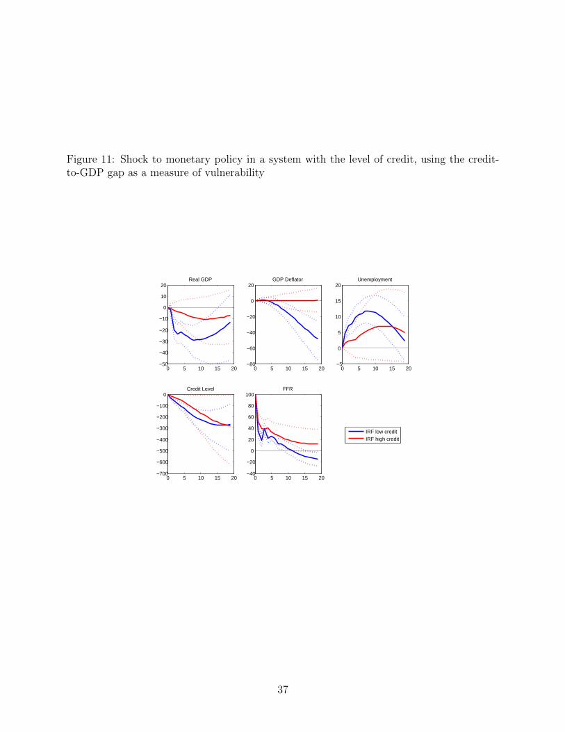
Figure 11: Shock to monetary policy in a system with the level of credit, using the credit-to-GDP gap as a measure of vulnerability

0 5 10 15 20−50

−40

−30

−20

−10

0

10

20Real GDP

0 5 10 15 20−80

−60

−40

−20

0

20GDP Deflator

0 5 10 15 20−5

0

5

10

15

20Unemployment

0 5 10 15 20−700

−600

−500

−400

−300

−200

−100

0Credit Level

0 5 10 15 20−40

−20

0

20

40

60

80

100FFR

IRF low creditIRF high credit

37

Figure 12: Credit shock using potential GDP to estimate the credit-to-GDP gap

0 5 10 15 20−300

−200

−100

0

100

200

300Real GDP

0 5 10 15 20−400

−200

0

200

400

600GDP Deflator

0 5 10 15 20−50

0

50

100

150

200Unemployment

0 5 10 15 20−100

0

100

200

300

400Credit/Potential GDP Gap

0 5 10 15 20−500

−400

−300

−200

−100

0

100

200FFR

IRF low vulnerabilityIRF high vulnerability

38

Figure 13: Response to a shock to household credit in a system with the credit-to-GDP gapdisaggregated between household and business credit.

0 5 10 15 20−100

−50

0

50

100

150

200

250Real GDP

0 5 10 15 20−100

0

100

200

300

400GDP Deflator

0 5 10 15 20−100

−50

0

50

100Unemployment

0 5 10 15 20−300

−200

−100

0

100

200

300Business Debt/GDP Gap

0 5 10 15 200

100

200

300

400

500Household Debt/GDP Gap

0 5 10 15 20−100

0

100

200

300

400FFR

IRF low credit IRF high credit

39

Figure 14: Response to a shock to business credit in a system with the credit-to-GDP gapdisaggregated between household and business credit.

0 5 10 15 20−100

−50

0

50

100

150Real GDP

0 5 10 15 20−100

−50

0

50

100

150GDP Deflator

0 5 10 15 20−40

−20

0

20

40

60Unemployment

0 5 10 15 20−300

−200

−100

0

100

200Household Debt/GDP Gap

0 5 10 15 20−100

0

100

200

300Business Debt/GDP Gap

0 5 10 15 20−100

−50

0

50

100FFR

IRF low credit IRF high credit

40

Figure 15: Impulse response to a monetary policy shock when the sample is divided intoperiods of increasing credit-to-GDP gap (red lines) and decreasing credit-to-GDP gap (bluelines).

0 5 10 15 20−60

−40

−20

0

20

40Real GDP

0 5 10 15 20−80

−60

−40

−20

0

20GDP Deflator

0 5 10 15 20−20

−10

0

10

20

30Unemployment

0 5 10 15 20−20

−10

0

10

20

30Credit/GDP Gap

0 5 10 15 20−20

0

20

40

60

80

100FFR

IRF credit declineIRF credit growth

41

Figure 16: Impulse responses to a shock to our constructed measure of risk appetite (ALLM)

0 5 10 15 20−5

0

5

10

15Real GDP

0 5 10 15 20−2

0

2

4

6

8GDP Deflator

0 5 10 15 20−6

−4

−2

0

2

4Unemployment

0 5 10 15 20−50

0

50

100

150risk appetite

0 5 10 15 20−6

−4

−2

0

2

4

6

8FFR

IRF low vulnerabilityIRF high vulnerability

42

Figure 17: Impulse responses to a shock to the negative excess bond premium (EBP)

0 10 20−1

0

1

2

3Real GDP

0 10 20−4

−2

0

2

4GDP Deflator

0 10 20−2

−1

0

1Unemployment

0 10 20−50

0

50

100OA EBP

0 10 20−2

−1

0

1

2FFR

IRF low vulnerabilityIRF high vulnerability

43

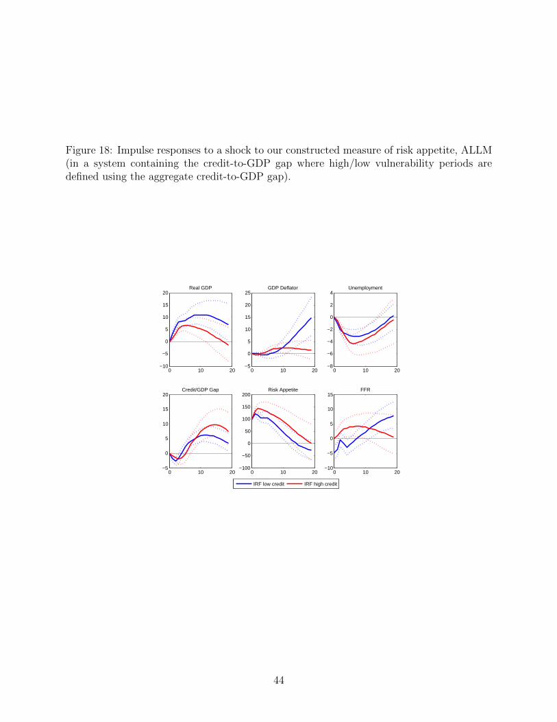
Figure 18: Impulse responses to a shock to our constructed measure of risk appetite, ALLM(in a system containing the credit-to-GDP gap where high/low vulnerability periods aredefined using the aggregate credit-to-GDP gap).

0 10 20−10

−5

0

5

10

15

20Real GDP

0 10 20−5

0

5

10

15

20

25GDP Deflator

0 10 20−8

−6

−4

−2

0

2

4Unemployment

0 10 20−5

0

5

10

15

20Credit/GDP Gap

0 10 20−100

−50

0

50

100

150

200Risk Appetite

0 10 20−10

−5

0

5

10

15FFR

IRF low credit IRF high credit

44

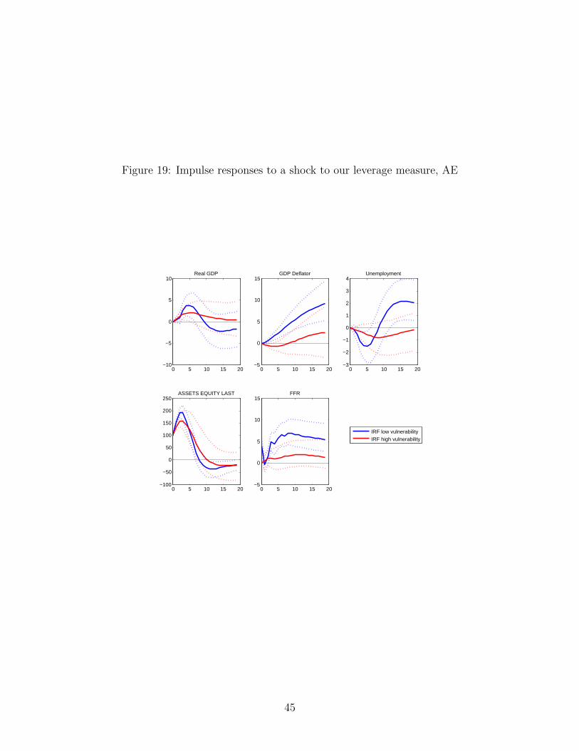
Figure 19: Impulse responses to a shock to our leverage measure, AE

0 5 10 15 20−10

−5

0

5

10Real GDP

0 5 10 15 20−5

0

5

10

15GDP Deflator

0 5 10 15 20−3

−2

−1

0

1

2

3

4Unemployment

0 5 10 15 20−100

−50

0

50

100

150

200

250ASSETS EQUITY LAST

0 5 10 15 20−5

0

5

10

15FFR

IRF low vulnerabilityIRF high vulnerability

45

Figure 20: Impulse responses to a shock to runnable liabilities estimated over the full sample.

0 5 10 15 20−20

−10

0

10

20

30

40Real GDP

0 5 10 15 20−80

−60

−40

−20

0

20

40GDP Deflator

0 5 10 15 20−15

−10

−5

0

5

10

15Unemployment

0 5 10 15 20−150

−100

−50

0

50

100

150Runnables/GDP Gap

0 5 10 15 20−150

−100

−50

0

50FFR

IRF low vulnerabilityIRF high vulnerability

46

Figure 21: Impulse responses to a shock to runnable liabilities estimated over the sampleafter the Bankruptcy Amendments Act of 1984 (1985:Q1–2014:Q4).

0 5 10 15 20−40

−30

−20

−10

0

10

20Real GDP

0 5 10 15 20−30

−20

−10

0

10

20GDP Deflator

0 5 10 15 20−5

0

5

10

15

20Unemployment

0 5 10 15 20−50

0

50

100

150Runnables Debt/GDP Gap

0 5 10 15 20−30

−20

−10

0

10

20FFR

IRF low vulnerabilityIRF high vulnerability

47