"%7"/$& MACROECONOMIC THEORY

Edited ByDr. Dilfraz Singh

MACROECONOMIC THEORY

Printed byLAXMI PUBLICATIONS (P) LTD.

113, Golden House, Daryaganj,New Delhi-110002

forLovely Professional University

Phagwara

SYLLABUS

Advance Macroeconomics Theory

ObjectivesTo give the students an overview of contemporary macroeconomic theory and to make the students understand and analyze relationships among different macroeconomic variables such as national income, employment, consumption, inflation and the quantity of money. Student will be able to understand the role of government expenditure, taxation and monetary policy in an economy.

S.No. Topics

1. Money multiplier and credit creation by commercial banks

Derivation, properties and shift in IS and LM curves.

Simultaneous equilibrium in money and product markets

2. Effects of monetary policies under different cases in IS-LM framework

Effects of fiscal policies under different cases in IS-LM framework

. Inflation: Types and its effects

Philips curve analysis

Trade cycles: Meaning and types

Accelerator - Multiplier Interaction model

. Kaldor’s model of trade cycles

Monetary and fiscal policy – Objective, conflicts

Mudell Model

. Swan Model

Rational Expectations and Economic Theory , New Keynesian Macro economics

Tanima Dutta, Lovely Professional University


3Pavitar Parkash Singh, Lovely Professional University




7Tanima Dutta, Lovely Professional University

8Tanima Dutta, Lovely Professional University


10Hitesh Jhanji, Lovely Professional University



13Ashwani Panesar, Lovely Professional University

14Ashwani Panesar, Lovely Professional University

Unit-1: Money Multiplier and Credit Creation by Commercial Banks

ContentsObjectivesIntroduction1.1 Money Multiplier1.2 Expansion of Credit Money or Credit Creation1.3 Some Basic Concepts1.4 Process of Credit Creation or How do Banks Create Credit?1.5 Limitations of Credit Creation1.6 Competitive Banking and Credit Expansion1.7 Do Banks Really Create Credit?1.8 Money Supply in India1.9 How does Money Get into the Economy?1.10 Does Supply of Money in the Economy Depend on the Discretion of the Central Bank?1.11 Summary1.12 Keywords1.13 Review Questions1.14 Further Readings

Objectives

After studying this unit, students will be able to:

Know the Money Multiplier, �

Know the Algebraic Expression, �

Know the Supply of Money in India, �

Know the Limitations of Credit Creation �

Introduction

Through credit creation, banks increase the supply of money in the economy which has a direct impact on production, consumption and level of investment and along with it process of development and prosperity is influenced.

Money Multiplier1.1

Money multiplier is the ratio of change in supply of money to the change in monetary base. Monetary base is the sum of currency in circulation and cash reserve of the banks. Consider that if as a result of a change of `. 10 crores in monetary base, there is a change of `. 30 crores in the supply of money

Notes

LOVELY PROFESSIONAL UNIVERSITY

Unit-1: Money Multiplier and Credit Creation by Commercial BanksTanima Dutta, Lovely Professional University

1

then money multiplier will be 3. Coefficient of Money multiplier may be known from the below mentioned formula:

Money Multiplier = Money SupplyHigh Powered Money

OR

MmH

= ....(i)

(Here, m = Money Multiplier, M = Supply of Money (currency in circulation and bank’s demand deposits), H = High power money)

Total Supply of money is the sum of currency and demand deposits.

M = C + D …(ii)

(Here C = Currency, D= Demand Deposits)

� Difference between M and H

M = Supply of money in which currency and demand deposits are included.

H = High Powered money which includes currency and reserves of commercial banks.

In cash reserve only includes required minimum reserves of the commercial banks and excess reserves.

Notes Money multiplier is the ratio of change in supply of money and change in monetary base.

Total supply of high powered money is equal to the sum of currency, required reserves of the banks, other deposits of the banks and excess reserve with the central bank.

H = C + RR + ER ...(iii)

(Here H: High powered money, C: Currency, RR: Required reserve of the commercial banks, ER: Excess reserve with the central bank)

If in equation (i) we substitute M and H we will get the below mentioned equation:

M = M C DH C RR ER

+=

+ +

Divide the right side of the equation with D (Demand deposits)

m =

C DM D D

C RR ERHD D D

+=

+ + ...(iv)

If in equation (iv), in place of CD

, we write c, in place of RRD

, we write r and in place of ERD

, we write e, then

Notes


Advance Macroeconomic Theory

2

(a) Money Multiplier

m = M 1 CH c r e

+=

+ + (v)

(b) Supply of Money= Money Multiplier X High Power Money

m = C D

M D DC RR ERHD D D

+=

+ +

....(vi)

(c) High Powered Money

H = Mm

....(vii)

In short, supply of money is influenced by money multiplier.

Self AssessmentFill in the blanks:

Monetary base is the .................... of currency in circulation and cash reserve of the banks.1.

By giving loans, banks want to earn more and more .................2.

Expansion of Credit Money or Credit Creation1.2

According to the above mentioned discussion, money supply in an economy depends on circulation of currency and demand deposits of commercial banks. Due to any increase in these two components, money supply in the economy increases. Quantity of currency is decided by the central bank which depends on the government’s nature of spending whereas deposit constituent of money supply is influenced by commercial banks. Commercial banks influence the money supply in the economy by credit creation or expanding credit money. Credit expansion capacity of commercial banks depends on their cash reserve ratio. In the words of Lipsey and Chrystal, “Banks can create money by issuing more promises to pay (deposits) than they have cash reserve available to pay out”.

In the words of Newlyn, “Credit Creation refers to the power of commercial banks to expand secondary deposits either through the process of making loans or through investment in securities.”

As per G.N. Halm, “The creation of derivative deposits is identical with what is commonly called the creation of credit."

Did You Know? Quantity of currency is decided by the Reserve bank.

Before analysing the process of credit creation knowledge of some basic concepts will be useful for the readers.

Some Basic Concepts1.3

Those deposits of the bank, which the depositor may withdraw anytime by drawing a 1. cheque, are known as demand deposits. It s also known as ‘Chequing deposits’ or ‘Chequable deposits’. Its detailed classification is as follows:



Notes

3

Primary or Cash Deposits: (i) The amount of money which is deposited by the people in form of cash in the banks is known as Primary or Cash Deposit. It is also known as passive deposits because banks have no role in developing these deposits. Amount of these deposits completely depends on the will of the depositor.

Derivatives or Secondary Deposits:(ii) When a person takes a loan from the bank, bank does not give him this loan in form of cash but opens an account in his name and gives him a right to withdraw money from it through cheque. Such deposit is known as Derivative or Secondary deposit. Hence each loan given by bank creates a new deposit. Secondary deposit is the result of primary deposit because banks create secondary deposit by keeping a part of primary deposit itself in reserve. According to Halm, "Creation of secondary deposit is credit creation; larger the amount that a bank advances greater is the creation of secondary deposits or loans created." That is why it is said, “loans create deposits and deposits create loans.”

Demand Deposits = Primary Deposits + or Secondary Derivative Deposits

Cash Reserve Ratio:2. No doubt that banks want to earn more and more profits by giving loan but it does not mean that it may lend its entire cash. The people who deposit their money in bank may withdraw it anytime because it is their money. hence banks alsways keep a part of net deposits in form of cash reserve with them, so that the requirement of the depositors may be fulfilled. That part of net deposit which banks keep with themselves as cash is known as Cash Reserve Ratio.

Excess Reserves: 3. The amount with the bank which is more than the required cash reserve ratio (CRR) is known as Excess Reserve. In reality, it is this excess reserve which becomes the base of credit creation.

Credit Multiplier:4. Ratio of increase in primary deposit and increase in total deposit is known as credit multiplier. If as a result of an increase of Rs. 1000 in primary deposits, there is a credit creation of Rs. 10,000, credit multiplier will be 10. Inverse relation between credit multiplier and Cash Reserve Ratio(CRR) may be expressed in form of following equation:

Credit Multiplier = Cash Reserve Ratio

1

Difference between money multiplier and Credit Multiplier

Money multiplier: It is the ratio of supply of money and high powered money.

m = 1 cc r e

++ +

Credit Multiplier: It is the ratio of increase in total deposits and increase in primary deposits of the banks or is the reciprocal of Cash Reserve Ratio (CRR).

Credit multiplier

D 1P r

Δ=

Δ

Here, r= Reserve ratio, D = Total Deposits, P = Primary deposits.

Self Assessment Multiple Choice Questions:

Creation of secondary deposit itself is —3.

(a) Credit creation (b) Credit

(c) Deposit (d)None of these



Notes

4

Loans do of deposits—4.

(a) Selection (b) Creation (c) Credit (d) None of these

Ratio of increase in primary deposits and increase in total deposits is called—5. (a) Credit multiplier (b) Credit (c) Multiplier (d) None of these

Excess reserve itself becomes of the credit creation—6. (a) Base (b) Budget (c) Multiplier (d) None of these

Process of Credit Creation or How do Banks Create Credit?1.4

Commercial banks’ method of credit expansion is based on the following conditions: Stability in Cash Reserve ratio of banks:(i) Cash reserve ratio of net commercial deposits of banks, remain constant during the period of credit creation process.No flow of cash:(ii) Excessive flow of cash should not happen from the banking system i.e. people should keep a designated amount of currency with them for exchange.

Study of process of credit creation can be done in two parts:(1) Single Banking System (2) Multiple Banking System

(1) Credit Creation in a single banking system

It is just an easy assumption that in an economy only one bank does all the banking business. Assume that MR. X deposits `. 1000 in the bank. In form of primary deposit, this amount is demand deposit of the bank. On this assumption that CRR is 10%, Bank’s balance Sheet will look like this:

Balance Sheet of the Bank (On primary deposit being ` 1000)

Liabilities AssetsDemand Deposits… .` 1000

(Primary Deposit)

Cash = ` 1000Cash Reserve fund = ` 100 (10% of 1000)Excess Reserve = 1000 – 100 = ` 900

Total = ` 1000 Total = ` 1000

Without liquidity or security risk, bank can give a loan of ` 900. If bank does so, its explanation will be as follows:

Balance Sheet of the Bank (When initial excess reserve is converted to

loan)

Liabilities Assets(i) Demand Deposits (Primary Deposit) `. 1000(ii) Demand Deposits = ` 900 (Secondary and derivatives deposits)

(i) Cash received = ` 1,000Cash Reserve fund (10% of 1000) = ` 100Excess Reserve = 1000-100 = `900(ii) Loan = ` 900

Total = ` 1,900 Total = ` 1,900



Notes

5

Where does the loan amount of ` 900 go? If the person taking the loan give the cheque of ` 900 to some other person (who has an account in the same bank), then there is no disturbance in bank’s cash reserve of ` 1000. Bank’s demand deposit becomes 1900 for which it needs cash reserve

fund of ` 190 10 1,900100

⎛ ⎞×⎜ ⎟⎝ ⎠

. In such situation, bank is left with an excess reserve of ` 1000 – 190 =

` 810. For bank it will be possible to give another loan of ` 810. Accordingly, bank’s demand deposit will increase to Rs.1000 + 900 + 810 = 2710. If the person taking the loan gives the cheque of ` 810 to another person (who has an account with the same bank), there will be again no disturbance in bank’s cash reserve of ` 1000. Bank, by keeping ` 271 (10% of 2710) in cash reserve fund, for demand deposit of ` 2710, will be able to give its excess reserve of ` 729 (1,000 – 271) in form loan to some other person. This process of giving loan by the bank will go on until excess reserve becomes zero. At the end bank’s balance sheet will be as follows:

Balance Sheet of the Bank (When excess reserve ends completely)

Liabilities AssetsDemand Deposits

(i) Primary Deposit = ` 1,000

(ii) Secondary and derivatives deposit = ` 900

` 810

` 729

(i) Cash received = ` 1,000

(ii) Loan = ` 900

= ` 810

= ` 729

This cycle will go on until excess fund does not become zero

Total = ` 1,0000 Total = ` 1,0000

In this manner, on the basis of cash received of ` 1,000, bank created demand deposits of ` 1,0000.

1 11,000 1000 Rs.10,000CRR 10%

⎛ ⎞× = × =⎜⎝ ⎠

because in this example, credit multiplier is 10.

Credit multiplier 1 1 10

CRR 10%= = =

There is an increase of ` 10000 in supply of money/ credit in the economy.

Conclusion: On an initial increase of ̀ 1,000 in bank’s demand deposit (in form of primary deposit) and on the basis of assumption of CRR to be 10%, bank’s demand deposit (sum of primary and secondary deposits) will increase to ` 1,0000.

Algebraic Expression

Algebraic expression of credit creation process as following:

ΔD = ΔP + ΔP (1 – r) + ΔP (1 – r)2 + ΔP (1 – r)3 +...........

= ΔP {1 + (1 – r) + (1 – r)2 + (1 + r)3 +.........}

Where, ΔD: Net change in demand deposit because of initial change of primary deposit.

ΔP: change in Primary deposit

r: Cash Reserve Ratio (CRR)



Notes

6

Continuing the above example where ΔP = ` 1,000 and r (CRR)= 10%, process of credit creation will be as such:

ΔD = ΔP +ΔP (1 – r) + ΔP (1 – r)2 + ΔP (1 – r)3 +...........

= 1,000 + 1,000 (1 – 10%) + 1,000 (1 – 10%)2 ............

= 1,000 + 1,000 × 910

⎛ ⎞⎜ ⎟⎝ ⎠

+ 1,000 × 29 ..........

10⎛ ⎞ +⎜ ⎟⎝ ⎠

= 1,000 29 91 .........

10 10

⎧ ⎫⎪ ⎪⎛ ⎞+ + +⎨ ⎬⎜ ⎟⎝ ⎠⎪ ⎪⎩ ⎭

= 1,000 × 1

9110

− = 1,000 ×

110 9

10−

= 1,000 × 10 = ` 1,000In this way an initial primary deposit of ` 1000, creates a credit of ` 10000 in the economy, here cash reserve ratio is 10 percent and there is no excess (unnecessary) flow of cash from the banking system. This process of credit creation is shown through figure 17.1.

In Figure 17.1 axis X deposits and axis Y measure various deposit rounds happening due to primary deposit. Primary deposit is ̀ 1,000 in the first round and net deposit is also ` 1,000. Initial deposit of ` 1,000 creates deposit of ̀ 9,00 in second round and ` 8,10 in third round. In this manner, this round of deposit creation will go on until all primary deposits are not divided in cash reserve ratio.

(2) Credit Expansion in Multiple Banking systemCredit expansion process in multiple banking system, though the medium of providing loan, is like single banking system only, which we have discussed earlier. Will ananlyse credit expansion by using the visualized equilibrium letter (Kalpit santulan Patra) of various commercial banks. Here banking system increases it multiple credit creation when all banks increase their deposit amounts with each other. In comparison to single banking system, credit expansion Process in multiple banking system is more realistic.

Assume that in an economy, A, B, C, D many banks are found. Firstly as person deposits ` 1,000 as primary deposit in bank A. In such situation, balance sheet of bank A will be as follows:

Initial Balance Sheet of Bank 'A'

Liabilities ` Assets `

Deposits 1,000Reserves

1,000

Total 1,000 Total 1,000

Figure 1.1

Deposit (`)



Notes

7

Bank A, keeping the cash reserve fund of 10%, gives ` 900 as loan. In such situation, final balance sheet of bank A will be as follows:

Final Balance Sheet of Bank 'A'


Deposits 1000Reserves

Loans

100

900

Total 1000 Total 1000

Assume that a person takes a loan of ` 900 from bank ‘A’ and gives a cheque of ` 900 for paying off debt, to another person who has an account on bank B. then initial balance sheet of bank B will be made as follows:

Initial Balance Sheet of Bank B

Liabilities ` Assets ` Deposits 900 Reserves 900

Total 900 Total 900

Bank B, after keeping 10 % of primary deposit of ` 900 as cash reserve ratio, gives balance ` 810 as loan. The final balance sheet of the bank will be as follows:

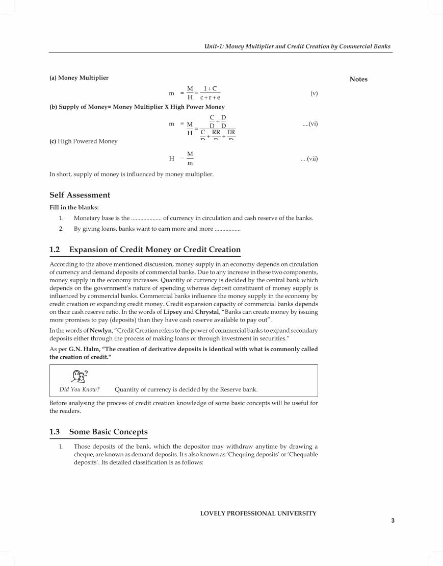
Final Balance Sheet of Bank 'B'



Loans

90

810Total 900 Total 900

A person borrows ` 810 from bank ‘B’ and for repayment of debt, gives a cheque of ` 810 to some other person who has an account with bank C. in such situation, initial balance sheet of bank C will be made as such:

Initial Balance Sheet of Bank 'C'


Deposits 810 Reserves (CRR) 810

Total 810 Total 810

Bank C, after keeping 10 % of primary deposit of ` 810 as cash reserve ratio, gives balance ` 729 as loan. The final balance sheet of bank C will be as follows:



Notes

8

Final Balance Sheet of Bank 'B'



Loans

81

729Total 810 Total 810

This process of credit expansion will go on until primary deposit of ̀ 1000, does not get distributed in the complete banking system in form of reserve fund. All banks will collectively create a new deposit worth ` 9000 and deposit of total banking system will be ` 10000 as is shown by table 1.1

Table 1.1

Bank New Deposits CRR New Loans

A

B

C

Other bank

1,000

900

810

729

-

100

90

81

-

-

900

810

729

-

-Total for the Banking System

1,0000 1,000 9,000

Change in Total Deposit = Primary Deposit X Credit Multiplier

Credit Multiplier 1 1 10

CRR 10%= =

Change in total deposit = 1,000 × 10 = 1,0000

In short, total deposit of complete banking system, because of the primary deposit of ` 1,000, will become ` 1,0000.

Task Express your thoughts in relation to money multiplier.

Limitations of Credit Creation1.5

Banks cannot create credit in unlimited quantity. There are many limitations to the credit creation power of commercial bank, details of which are as follows:

Cash Reserve Ratio:1. Power of credit creation mainly depends on cash reserve ratio (CRR). There is a mutually inverse relation between credit creation and cash reserve ratio. As much cash reserve ratio will be more, creation of credit will be as less. As opposed to this,


Unit-1: Money Multiplier and Credit Creation by Commercial BanksMacroeconomic Theory

Notes

9

as much less will the cash reserve ratio be that much more will the creation of credit be. For example,

Cash Reserve Ratio (r) Primary DepositIncrease in Total Deposit

1D Pr

⎛ ⎞Δ = Δ⎜ ⎟⎝ ⎠

Credit Creation

10%

5%

20%

1,000

1,000

1,000

10,000

20,000

5,000

10,000 – 1,000 = 9,000

20,000 – 1,000 = 19,000

5,000 – 1,000 = 4,000

(Here, ΔP: increase in primary deposit; ΔD: increase in total deposit; r = cash reserve ratio.)

It is clear from the above example that when cash reserve ratio (r) will be 10 percent, then increase in total deposit will be ` 1,0000. When cash reserve ratio will increase to 20 percent, then increase in total deposit will be just ` 5,000. Opposed to this, when cash reserve ratio decreases to 5 percent then increase in total deposit will be ` 20,000.

Amount of Primary Deposits: 2. Expansion of Credit creation depends on the quantity of primary deposit. There is a direct relation between credit creation and primary deposit. If quantity of primary deposit is more, creation of credit will also be more and if quantity of primary deposit is less, creation of credit will also be less, even if cash reserve ratio remains constant. For example, if

ΔP = ` 1,000; r = 10% ⇒ ΔD = ` 10,000

ΔP = ` 5,00; r = 10% ⇒ ΔD = ` 5,000

ΔP = ` 2,000; r = 10% ⇒ ΔD = ` 20,000

If Cash reserve ratio (r) is 10%, then form a primary deposit of ` 1,000, total deposit of ` 10,000 may be obtained. At the other end, primary deposit just left to be ̀ 5,000, total deposit can only increase to ` 5,000. If primary deposit is ` 2,000, total deposit may increase up to ` 20,000. Hence we reach the conclusion that if cash reserve ratio (r) remains constant, then there is a mutual direct relation between primary deposit and total deposit.

Banking Habits of the People:3. Bank’s power of creating credit also depends on banking habit of the people. If people do their business mainly through cheque, they will need to keep very little cash with them. As a result cash with the banks will increase because of which, their power of credit creation will also increase. In developed countries of the world, it happens the same way. But in undert-developed countries, people mainly do their business through cash. As a result, their demand for cash is always more. Because of this, cash balance of banks reduces and along with it their power to create credit also reduces.

Credit Policy of the Central Bank: 4. Power of commercial banks to create credit also depends on credit Policy of the central bank of the country. If the central bank follows cheap credit policy (credit expansion policy), credit creation power of the commercial banks increases; as opposed to this, if the central bank follows expensive credit policy (controlled credit policy), credit creation power of the commercial banks reduces.

Policy of Other Banks:5. Power of credit creation by one bank also depends on credit policy adopted by other banks. If all banks work in the same tune then their power of credit creation will be more. But if one bank expands credit but other banks do not co-operate with it then process of credit creation will be limited.



Notes

10

Confidence of Depositors: 6. Power of commercial banks to create credit is also influenced by the confidence of the depositors. If depositors have full faith on the banking system then they will let their money lie in the bank. It will increase the credit creation power of the banks. As opposed to this, if people do not have faith in the banking system then they will not keep their savings in banks. Less amount of cash balance with the banks reduces their credit creation power.

Availability of Good Borrowers:7. Availability of borrowers worth credit also influences credit creation power of the banks. If such borrowers are available in big numbers then more credit will be created. If good borrowers are not available banks will hesitate in giving loans and credit creation will be limited.

Commercial and Industrial Conditions:8. During the period of recession, businessmen’s and industrialists’ demand for loan is very less. Hence not much credit is created by banks in form of secondary deposits. But during boom period, giving loans is profitable for the banks and they create more credit in form of secondary deposits.

Two principal parameters that Delimit the Credit Creation Capacity of the Commercial Banks

Two principal parameters that delimit the Credit Creation Capacity of the Commercial Banks are as follows:

Primary deposits of commercial banks or cash reserves: (i) As much more will be cash reserves that much more will be the power of the banks to create credit.

Cash reserve ratio determined by the central bank:(ii) It is compulsory for the commercial banks to follow the orders of the central bank, relating to Cash Reserve Ratio (CRR). If CRR is increased as in situation of inflation, credit creation power of banks is contracted. As opposed to this if cash reserve ratio is reduced, as in the condition of recession, then credit creation power of the banks increase a lot.

Self AssessmentState whether the following statements are True or False:

Money Supply in an economy depends on velocity of currency and demand deposits of the 7. bank.

Credit expansion capacity of commercial banks depends on their cash reserve ratio.8.

That deposit of the bank is called the demand deposit which the depositors cannot withdraw 9. anytime by issuing a cheque.

Supply of money and high powered money is retio. 10.

Competitive Banking and Credit Expansion1.6

Like Joint stock companies commercial banks also work for profit. According to the perspective of credit expansion, commercial banks through the medium of credit expansion, want to maximise their profits. But credit expansion is not always possible. If people decide to make an increase in their primary deposits then, commercial banks will be able to increase their secondary deposits. Banks, with the help of the primary deposits of the people, increase secondary deposits and expand credit. But in current competitive age, commercial banks, in order to maximise their profits and for expanding credit try other measures. Banks keep excess reserves with them which fulfil the increasing credit requirement in money market. For expanding credit and increasing profits commercial banks plan their policies demand and supply Parameters of money market.



Notes

11

Figure 1.2

In competitive banking system quantity of credit of banks is determined by demand for loans and supply of loans. Demand for loan depends on the prevailing interest rates and supply of loan depends on quantity of deposit and spread of interest rates What interest rate banks give for accepting deposits from people and what interest rate banks charge for giving loans to the people, the difference between it is known as spread of interest rates. Spread of interest rate is decided by loan supply line and deposit supply line. Demand for loan is inversely related with interest rates. Excessive interest rate reduces demand for loan and less interest rate increases demand for loan. In this manner loan demand curve is a downward falling line. Supply of loan and supply of deposit is directly related to rate of interest. On high interest rates banks do a greater supply of money and people deposit more cash in banks. Slope of both loan supply and deposit supply line is upwards.

In figure 1.2, SL is line for supply of loan; Sd is line for supply of deposit. DL is the demand curve of loan. Balanced Rate of interest is Or where DL = SL. It is that rate of interest which bank receives for giving loan to the people. Or1 is that rate of interest which bank gives to the people on deposit amount. Difference between both interest rates rr1 (spread of interest rate) determines the quantity of loan supply by the banks.

In the figure, interest rate spread is assumed to be constant that is why loan supply curve and deposit supply curve are mutually parallel. Quantity of loan supply by the banks depends on interest rate spread and deposit supply. Undoubtedly, when there is a boom in money market then for adjusting supply of loan and demand of loan, excess reserves of the bank have a very important role.

Do Banks Really Create Credit?1.7

There is a difference of opinion found among the economist that in reality whether credit is created by banks or depositors. Walter Leaf and Cannon’s opinion is that banks do not themselves create credit. Depositors do the job of credit creation who through their deposits, provide monetary resource to the banks. One part of this deposit is given by the banks as loan. This loan is helpful in credit creation. If depositor does not deposit his money in bank, bank will not be able to create credit. Bank may be compared to a cloak room. Assume that, in a party 50 guests come with simmilar overcoats which they deposit in a cloak room. Also assume that party will continue till 12 O’ Clock. Watchman of the cloak room keeps 10 overcoats with himself and gives the rest 40 overcoats to other people on rent for until 11:30 at night. He has kept 10 overcoats with himself because if some people want to go from the party before 12 O’Clock then he may give them these coats. Thus in this manner, by giving 40 overcoats for rent, has the watchman created 40 new overcoats? It is absolutely wrong. In the same way bank also by lending the money of the depositors, does not create credit. Keeping this in mind, Cannon has said, "The talk of credit creation by banks is all moon-shine and that every practical banker knows that he is not a creator of credit or money or anything else but a person who facilitates the lending of resources by the people who have them, to those who can use them."

But according to modern economists, above thought of Walter Leaf and Cannon is not correct, because banks lend money more than primary deposit. That is why, it will have to be accepted that banks create credit. Hartley Withers have rightly said, "Loans make deposits and the initiative of creating them goes to the banks."

Notes



12

Lipsey and Steiner also believe that expansion of credit is not automatic. It depends on decisions of banks. If banks do not use the increase in cash reserve fund, expansion of credit may not happen.

Money Supply in India1.8

Since 1977, RBI in india is using four monetary aggregate measures which are M1, M2, M3, M4. M1 is a narrow measure while M3 is a detailed measure of money supply. Since the first five year plan till today, there is a rapid increase in both M1 and M2. In currency component and bank deposit components of money supply, in both there has been a rapid increase. In the initial years of the plan, increase in currency component was more that deposit component. But at present time, in comparison to currency component, increase in demand deposit component is much faster; its main reason is extensive increase in banking services. Table 1.2 shows increase in M1 and M3 aggregates of money supply.

Table 1.2 Money Supply (M1 and M2)

Year (1) M1 (2) M3 (3)

1970-711980-811990-912000-022004-052005-062006-07

7,32123,11792,892

4,22,8436,46,2638,26,3757,65,195

10,95855,358

2,65,82814,98,35522,33,16427,29,54533,10, 278

(Source : RBI Bulletin 2006, Statistical Outline of India, 2007-08)

From table 1.2 it is clear that from 1970-71 to 2006-07, increase in M1 and M3 happened with a rapid speed. Rapid increase of M3 (approximate 302 times) happened due to increase in time deposits. Extensive increase of M1 happened due to increase in demand deposits.

Knowledge of Supply of money in India during various plan periods, national income and percentage increase in price levels can be obtained through table 1.3:

Percentage Growth Rate in Money Supply, National Income and Price Level

Period Growth Rate in Money Supply (M3)

Growth Rate in National Income

Growth Rate in Price-

LevelFirst PlanSecond PlanThird PlanFourth PlanFifth PlanSixth PlanSeventh PlanEighth PlanNinth PlanTenth Plan(2002-03)

2.25.39.115.517.916.717.513.814.216.4

3.74.12.43.35.05.45.75.85.68.7

-3.6+6.3+5.8+9.0+6.3+9.7+6.7+6.6+3.9+5.2

(Source: Statistical Outline of India, 2007-08)



Notes

13

This general belief has been found that there is an intense relation between supply of money and price level. When there is an increase in supply of money then through increase in demand prices also increase. Undoubtedly, supply of money has a direct influence on prices but it is difficult to agree with this opinion of Irving Fisher, the main supporter of Quantity Theory of Money, that there is a direct and proportionate relation between quantity of money and price level. For example, in the above given table it is shown that during the period of first plan, there was a fall in price level whereas money supply increased. During the period of ninth plan, in price level there was an increase of only 3.9 percent, whereas in supply of money, there was an increase of 14.2 percent. In an under developed country like India, a large pat of the economy is un-monetized. In this field, all transactions are done on the basis of exchange of goods. If one part of supply of money is used for monetization of this field then demand will increase by this but there will be no increase in prices. Hence in under developed countries like India, if increase in supply of money is used for increasing production and for monetization of non-monetized areas, then prices will not increase.

Form the above table, it is known that supply of money does have in influence on prices but there is no special relation between these two. How increase will be there in prices, as a result of increase in supply of money, this depends on many factors, especially on increase in production in the economy. According to Prof. B.N. Pandit, almost a time lag of one year is found in increase in supply of money in India and its influence on prices. During the period of plans, average rate of increase in supply of money was 14 per cent whereas rate of growth (on increase in national income) was 4.1% and increase rate (growth rate) of price level had been 6.6%.

How does Money Get into the Economy?1.9

How does a unit of money get into the economy? It is an important question which a student of economics should understand. In most countries of the world central bank issues notes and coins. For a general person, central bank (RBI in India) prints money and introduces it in the economy. But on which conditions and under what circumstances central bank prints money and introduces it, this question is not as easy as a general person thinks.

Government, for fulfilling budgetary loss, takes loan from the central bank (RBI) by giving its security. Central bank, by printing more money, gives loan to the government and government spends this loan on various developmental and non-developmental works. People may find their income in form of tax (Lagan), labour, profit and interest, from expense done by the government on various projects. In this form currency is introduced in the economy.

As per Lipsey and Chrystal, ‘The central bank gets high powered money into the economy simply by buying securities (usually government debt instruments). It pays for these purchases with newly issued high powered money."

Does Supply of Money in the Economy Depend on the Discretion 1.10 of the Central Bank?

No, Supply of Money in the economy does not depend on the discretion of the central bank. No doubt that the central bank (RBI) of the country is officer for issuing the currency of the country. But net sypply of money does not only depend upon the discretion of the central bank. Nte supply of money in an economy depends on the nature and will of the below given factors of the economy:-

(i) Central bank of the country (ii) Commercial bank of the country (iii) General Public.

Deciding the quantity of high power money which does the job of money multiplier, central �banks does determines its supply.

Notes



14

By determining its Cash reserve ratio (CRR), which is the base of credit multiplier, commercial �banks influence the supply of money.

General public, by determing their preference for liquididty, influence the supply of money. �It determines the cash reserve ratio of commercial banks and their power to create credit.

Velocity of money should not be ignored. It means that how many times, one unit of money (like a note or a coin) is used as a means of exchange. If velocity of money is measured in form of per unit time-period or in form of flowing concept then, it will also be an important determinant of money supply.

Ideal Supply of Money

Supply of money has an influence on net expenses. Consequently, trade activities, production and employment, all are affected by this. The question arises that for purchasing products produced by an economy will full employment, in which not source of production is wasted, how much money is needed? this supply of money itself is known as ideal supply. As a result of this supply, it becomes possible to completely utilize the production capacity of the country. In a situation of full employment, if supply of money exceeds ideal supply, condition of inflation arises and prices will rise sharply. As opposed to this, if supply of money is less than ideal supply then prices will start declining, depression will be there and unemployment will be there all around. Hence supply of money should be such so that in the country, all those goods which are being produced may be purchased so that condition of inflation or deflation may not be created.

It must be kept in mind that influence of supply of money on total expense will only be there when people will spend money and not keep it with themselves in form of cash. In reality, by change in supply of money there is also a change in liquidity of the people. People keep their assets in form of monetary, financial and actual fund with themselves. As a result of change in supply of money, changes also happen in monetary assets of the people. If due to change in monetary assets people will want to spend more money on actual assets like house, car, TV set etc, then total expense, and along with it national income will increase. As opposed to this, if people will want to spend their money on financial assets like shares, securities etc. then their prices will rise and rate of interest will decline. Low rate of interest will encourage investment and national income will rise. But if people will prefer to keep their increased monetary assets in liquid form, then there will be no change in total expenditure and nor will the national income change. Hence only by change in supply of money objective of price stability or full employment cannot be achieved. Calculating people’s demand for money is equally important.

Key Points

Money Supply: � It shows the quantity ofmoney available in the economy for business. It is a stock concept which is measured on a definite time.

Components of Money Supply: � (i) Currency (ii) Demand deposits.

Monetary Aggregates used in India: � According to old measures it is M1, M2, M3 and M4. According to new measures it is NM2, NM3, L1, L2 and L3.

Factors Influencing Money Sup � ply: (i) Size of monetary base (ii) Ratio of cash and demand (iii) Velocity

Students are advised that they read this paragraph carefully so that they may have knowledge about how supply of money affects the financial activities in an economy.

Notes



15

Money Multiplier: � It is the ratio of change in money supply and change monetary base.High Powered Money: � It is that money which is issued by central bank or government and is kept with themselves by the public or commercial banks.Credit Multiplier: � It is the ratio between change in total deposit and change in primary deposit.Demand Deposit: � It is that amount kept by the people with the bank, which may be withdrawn any time through cheque.Primary Deposits: � Amount deposited as cash by the people in the bank is known as primary deposit. Derivatives or Secondary Deposits: � Derivative deposit is the result of primary deposit because commercial banks, keeping a part of primary deposit in form of money, create secondary deposit.Cash Reserve Ratio: � That part of total deposit which commercial banks keep with themselves as cash is known as cash reserve ratio.Excess Reserve: � Cash reserve that remains with the bank in excess of cash reserve ratio is known as excess reserve.Limitations of Credit Creation: � (i) Cash reserve ratio: on cash reserve ratio being more, quantity of credit creation redues. (ii) Amount of primary deposit: more primary deposit shows more credit creation capacity (iii) Banking habit of the people: by more use of banking services by people, more credit will be created. (iv) Credit policy of central bank: cheap credit policy of central bannks provides the facility of more credit creation (v) Credit policy of other banks: is all banks work united, more credit will be created (vi) Confidence of depositors (vii) Availability of good borrowers (viii) Commercial and industrial conditions. Principle Parameters that Delimit the Credit Creation Capacity of Commercial Banks: � (i) cash reserve of commercial banks (ii) cash reserve ratio of central bank.

Summary1.11 Velocity of money should not be ignored. It means that how many times, one unit of money �(like a note or a coin) is used as a means of exchange. If velocity of money is measured in form of per unit time-period or in form of flowing concept then, it will also be an important determinant of money supply.

Keywords1.12 Discretion— Will. �Non- Monetized— where there is no money. �

Review Questions1.13 What do you understand by money multiplier?1. Describe the limitation of credit creation.2. How does money get into the economy?3. Does sup4. ply of money in the economy depend on the dicretion of the central bank?

Notes


Answers: Self Assessment 1. sum 2. profit 3. (a) 4. (b) 5. (a) 6. (a) 7. True 8. True 9. False 10. True

Further Readings1.14

Books Macroeconomics—1. Mohan Srivastava, DND Publications, 2010.

Macroeconomics— 2. S.K. Chakravarty, Himalaya publishing House, 2010.


16

Unit-2: IS - LM Analysis

ContentsObjectivesIntroduction2.1 IS Curve and Its Derivation (Product Market Equilibrium)2.2 LM Curve and Its Derivation (Money Market Equilibrium)2.3 Summary2.4 Keywords2.5 Review Questions2.6 Further Readings

Objectives


Know the derivation of IS Curve, �

Know the derivation of LM Curve. �

Introduction

Now we’ll analyse the simultaneous determination of equilibrium GDP interest rate. Besides from equilibrium interest rate, equilibrium GDP presents a partial approach of complex economy equilibrium. Interest rate affects the investment level so to actual GDP level also. Similarly GDP level affects the interest rate in the economy by the demand of money. When interest rate is increasing then on special rise in investment, an economy can’t make a rise the GDP level till diversified range. Similarly interest rate can’t be reduced till the limit of extent of increase in money supply because increase in money supply (by low interest rate and high investment) and high GDP make an increment in supply of money, which means the increment in interest rate. Therefore, the Traditional/Classical view that interest rate is a real phenomenon and is determined by savings and investment only. And J. M. Keynes view that it is only a monetary phenomenon and it is determined by supply and demand of money, these both views are challenged. J. R. Hicks and Hensen have established a new approach by IS-LM Analysis, which integrates the real and monetary phenomenon both. The simultaneous determination of interest rate and actual GDP and the alternative derivation of AD curve is the cornerstone of IS-LM Analysis. In the determination of Actual GDP and Interest rate, because J. R. Hicks and Hensen synthesise both the real and monetary phenomenon, so their approach is called as Hicks-Hensen Synthesis. The equilibrium of IS-LM Curves means the determination on the equilibrium level of actual GDP and equilibrium interest rate by equality between investment and saving and equality between supply and demand of money. This approach of interest determination is called as the Modern Theory of interest rate determination. Current chapter explains how the IS and LM Curves are derived and how the balanced actual GDP and interest rate are determined. Besides it


Notes



17

we also derive the Aggregate Demand Curve from IS-LM Analysis and will concentrate on the thing that how the shift in IS or LM brings the shift in Aggregate Demand Curve.

Notes Interest rate affects the investment level.

IS Curve and Its Derivation (Product Market Equilibrium)2.1

The IS Curve shows that coincidence of interest rate and actual GDP which establishes the equality between saving and investment. According to, Lipsey and chrystal “The IS Curve is the locus of interest rate and actual GDP that are consistent with equality between desired spending and output, or what is the same thing, injection and leakages. It is drawn for given value of the government expenditure, exports, and automatic consumption as well as forgiven tax rates and a given price level.” Therefore the IS Curve or IS function indicates the commodity market equilibrium.

Two situations come in derivation of IS Curve. In first situation, the relation between investment and interest rate is established by investment demand function and in second situation; we’ll explain how the change in investment spending affects the actual GDP. On combining the interest rate and actual GDP, we’ll establish the equilibrium in commodity market.

I. The Investment Demand Function

Relationship between r and I

It means the inverse relationship between investment and interest rate. The desired rate of investment will be low on the high interest rate, and will be high on the low interest rate. The working relationship between investment and interest rate can be written as following-

I = Ia – br, b > 0

[Here I: Investment; Ia: autonomous investment; r: interest rate; b: the responsiveness of investment spending from interest rate.]

The above investment function shows that the means of low interest rate is high investment or vice-versa.

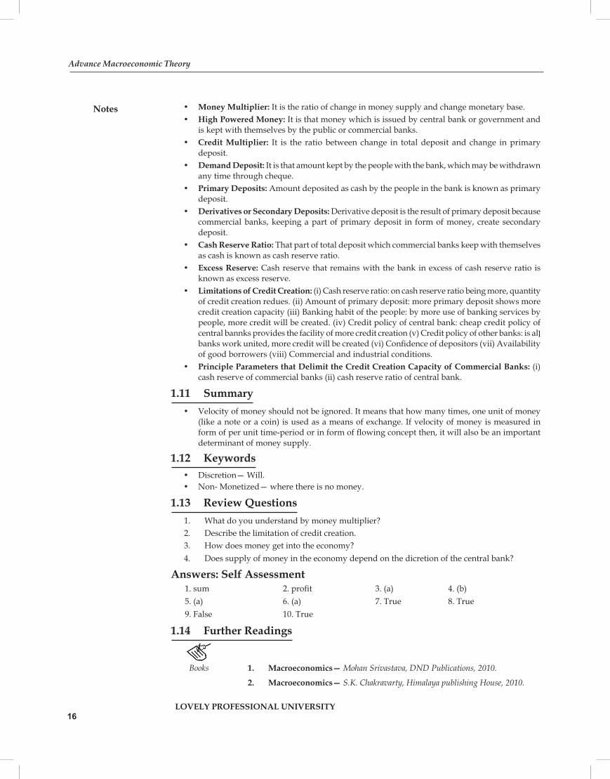
In figure .1, II1 is the investment demand curve, which shows the negative relationship between investment and interest rate. On the low interest rate ‘Or1’ , investment spending is ‘OI0’ and on high interest rate ‘Or’, it is ‘OI’. If there is any change in the autonomous component ‘Ia’ of investment, then there is a shift in investment demand. Rise in ‘Ia’, rise in II1 Rise in ‘Ia’ will shift the II1 Curve towards right and the reduction in it (Ia) will shift the II1 towards left.

Did You Know? The change in investment spending affects the actual GDP by the change in investment spending.

Notes



18

Figure .1 Figure .2

Figure – .1 shows that on the change in autonomous investment there is a shift in investment demand function. The rise in autonomous investment will convert the investment curve II1 into II2 on making a shift in it and the reduction in autonomous investment will convert the investment curve II1 into II3 on making a shift in it.

II. How investment affects Aggregate Expenditure and the level of GDP when ‘r’ happens to change?

Because of change in investment spending, there happens the change till the diversified range in total expenditure. According to Investment Multiplier Theory if the interest rate remains constant then the change in I can become the cause of the change in Total Spending (AE) and GDP. But if interest rate (r) doesn’t remain constant (As in IS-LM Model) then the process of investment multiplier would not be as easier. It is shown in figure .3 how the interest rate ‘r’ impacts on I and so impacts on total spending AE and the level of GDP.

The parts (A) and (B) of figure 3 show the relationship between equilibrium actual GDP and investment spending with the change in interest rate. Initial equilibrium is on point E where the rising in investment expenditure from I I to I1I1, the total expenditure in part A become AE1 on shifting from AE in AE = Y (Part A) and S = I (Part B). According to it, new balanced GDP should be OY1 where AE1 = Y and S = I1I1. But the rise in level of GDP increases the demand of money and so becomes a rise in ‘r’ in the situation of rise in interest rate, investment expenditure becomes low and so investment curve shifts from I1I1 to I2I2 towards backside. According to it, in part A, actual total expenditure on rising becomes AE2 instead of AE1. Actual GDP becomes OY2 instead of OY1. The high interest rate decreases the investment expenditure, which further decreases the total expenditure. If interest rate falls then vice-versa will be there. Therefore, the change in interest rate, by the change in investment expenditure, affects actual GDP.


We also derive the ………………………. demand curve from IS-LM Curve.1.

Because of change in investment spending, there happens the ……………… till the diversified 2. range in total expenditure.


Notes

LOVELY PROFESSIONAL UNIVERSITY19

III. Relationship between different levels of r and GDP on the one hand and the quality between S and I on other: IS Curve

We see that the balanced level of GDP is analogous to every level of ‘r’ that tells the homogeneous equality as similar to saving (S) and investment (I). You should be determinant that the work of high level of ‘r’ is the lower level of GDP and saving (S) and investment (I) is the analogous equality. On the other hand, the mean of the lower level of ‘r’ is the high level of GDP (Which happens by the high level of AE and I) and being the analogous equality between S and I.

In figure .4, the IS curve is shown which is derived from figure 18.4 (A). The IS curve shows that combination of actual GDP and Interest rate where the desired expenditures of economy are equal to total product. On the interest rate ‘Or’ given in Part-B, balanced actual GDP level is OY which is determined on making the line AE in part A and aggregate product line equal. This combination (OY, Or) of actual GDP and interest rate is shown by point A in part B. similarly point B is the combination of OY1 actual GDP level and Or1 interest rate in part B. The actual GDP level on Or2 interest rate is OY2, which is shown by point c in part B. We get the IS curve on joining these all combination points (as A, B, C) of actual GDP and interest rate. There every point on IS Curve shows the equilibrium in commodity market.

The points situated on the right or left of IS curve, show the imbalance in commodity market. If we take point M (In figure18. 4B) it is right from IS curve. It is known from this point that there is imbalance between AE and Y in part A. So total production is greater than total expenditure or the saving is greater than investment (Y > AE, ⇒ S > I). Similarly, any point on left of IS Curve, as point N, indicates that combination of GDP and Interest rate where total expenditure is greater than total production and investment greater than saving (AE > Y, → I > S).

Slope of IS Curve

The IS Curve is derived from the combination of actual GDP level and interest rate. It’s slope is downward from left to right. It means that high interest rate decreases the actual GDP because of less

Figure .3

Notes



20

investment expenditure and low interest rate increases the actual GDP because of high investment expenditure. Being the flatter or steeper of IS Curve depends on this thing how sensitive investment from the change in interest rate and how much is the price of multiplier. If investment is more sensitive from an specified change of interest rate then the IS Curve will be flatter. And if investment is less sensitive from an specified change of interest rate then the IS Curve will be steeper. The price of multiplier also determine to be steeper or flatter of IS Curve. In the situation of high multiplier price, because of an specified change in investment, the senstivity is larger (on a given interets rate). Because of this AE Curve is flatter which is responsible for being the IS Curve flatter. In the situation of being this multiplier price lesser, the AE Curve is steeper because of which the IS Curve is also respectively steeper.

In figure 2.5, the IS Curve is shown as negative sloped. The IS Curve is flatter for the high price of multiplier or interest rate sensitive investment as IS1. The IS Curve is steeper for the low price of multiplier or insensitive investment as IS2.

Two parameters impacting slope of IS Curve

Sensitivity of I to r:(i) The senstivity of I to r is as higher i.e., the responsiveness of investment towards the change in interest rate the IS Curve will be as flatter and vice-versa.

Value of Multiplier: (ii) The value of Multiplier is as higher i.e., because of rise in investment there is as rise in Aggregate Expenditure.

Shift in IS Curve

The shift in IS Curve happens because of the change in any analogous component of total expenditure. In two sided economy, it can happen because of change in analogous consumption expenditure and analogous investment expenditure. The rise in analogous investment expenditure shifts the IS Curve towards left. It’s cause is easy. The rise in analogous investment expenditure shifts the AE Curve parallely upward. The upward shift of AE Curve shifts the IS Curve towards right.

Figure .4


Notes


Part B of figure .6 shows that IS Curve becomes IS1 and IS2 on shifting from IS. The rise in exogenous expenditure (the analogous investment given by the government) shifts line AE (in part A) upward on AE1. Consequently, (On the constant interest rate Or) the IS Curve becomes IS1 on being shifted from IS (in part B). On reducing the analogous expenditure, the AE Curve becomes AE2 on being shifted downward from AE (in part A). Consequently, the IS Curve becomes IS2 on being shifted backward from IS (in part B).

Self AssessmentMultiple Choice Questions:

If there is a change in analogous component Ia of investment, then there will be a/an ........ 3. in investment demand curve.

(a) shift (b) inclination

(c) change (d) none of these

How investment impacts Aggregate Expenditure and the level of GDP when ‘r’ happens 4. to change?

(a) PGP (b) GDP

(c) ADP (d) Nome of these

If interest rate (r) doesn’t remain constant (As in IS-LM Model) then the process of investment 5. multiplier would not be as …………….

(a) easier (b) harder

(c) variable (d) none of these

The IS Curve is ..................from the combination of actual GDP level and interest rate.6.

(a) born (b) derived

(c) established (d) none of these

LM Curve and Its Derivation (Money Market Equilibrium)2.2

The LM Curve shows the different combinations of actual GDP (Y) and interest rate (r) which establishes the equality between supply and demand of money. Hance it shows the relationship between actual GDP and market rate of interest. According to —Lipsey and Chrystal. “The LM Curve plots combinations of GDP and the interest rate, for a given money supply and given price level, that are consistant with the equality of money demand and money supply.”

The derivation of LM Curve makes the study of all three relationships mandatory: (i) We establish the relationship between money demand and interest rate. (ii) We explain this thing how the change in GDP by the change in demand of money impacts the interest rate. (iii) On one hand, We establish the relationship between the different values of ‘r’ and GDP and on the other hand, establish the equality between demand of money and supply of money.

Demand of money and interest rate:(i) The purport from demand of money is the demand of real balance by the people. Real balances mean money balance or normal balance which are

Figure .5

Notes



22

combined with the changes occuring in the prices. So when price level becomes double then people keep the money in double quantity in themselves firstly so that their real balances (or purchasing power) remain constant. The demand of real balances in economy depends on two facts: (i)The GDP level and (ii) Interest rate. The GDP level is the clear determinor of real balances, because people keep the money to themselves for purchasing the goods and services. The high level of GDP means the high demand of real balances and vice-versa. The mean of interest rate is the oppurtunity cost of keeping the money himself. Because when you keep a fixed amount of money in cash form then you have to be deprived from that income gotten in interest form which you could get if you had invested this money in bonds purchase. In other words, the demand of cash balances are inversely related with interest rate (r) on a fixed GDP level.

The impact of ‘r’ and GDP in the reference of real balances is shown in figure .7.

The line L1 shows that demand of money is inversely related with ‘r’. On a fixed GDP level the high ‘r’ means the low damand of money (and vice-versa). Therefore when r = Or1 then the demand of money = OK and when ‘r’ becomes Or2 on reducing then the demand of money becomes OK1 on increasing. When ‘r’ remains constant, and there is a rise in GDP, then L1 – line becomes L2 on being shifted, it means that the rise in demand of money on a fixed level of ‘r’. So though ‘r’ = Or2 then also demand of money becomes OK2 on increasing from OK1 then GDP increases as shown by the shift of line L from L1 to L2.

(I) Impact of GDP changes on interest rates

Now we have known that the changes in actual GDP that the determination of interest rate done by the demand and supply of money. This fact that GDP level impacts on the demand of money and demand of money affects the interest rate, the contained GDP of these all is the found of situation of inter-relation between interest rate and demand of money. In figure .8, the stirring of this inter-relation is shown.

Note: The supply of money (Line M) is shown constant because it’s determination is independently done by monetary officials. It shows the real balances in economy. It is based on this recognition that price level remains constant.

Figure .6

Figure .7

Unit- : IS - LM Analysis

Notes


The balanced interest rate (Or) is determined on a fixed demand of money (L) and supply of money (M) on that point where L = M.

The demand rises with the rise in GDP, consequently the demand of money curve becomes L2 on being shifted from L1. Consequently the interest rate becomes Or1 on incresing from Or. Similarly, if there is reduction in GDP, then there will also reduction in demand of money, because of which the demand of money curve bacomes L3 on being shifted backward from L1. Consequently, the interest rate becomes Or2 on decreasing from Or. So the change in GDP, becomes the cause of change in interest rate by the change in demand of money.

Here the considerable thing is that the impact of change in GDP occurs only on the transaction demand of money not on speculative demand of money. We know that there is no any direct relationship between transaction demand of money and ‘r’; then why is ‘r’ being affected from the change in GDP? The fact for this is so: when transaction demand of money rises (because of rise in GDP) then when does the money come from? Because it is our recognition that supply of money remains constant (as shown in the vertical straight line in the figure). The pressure of transaction demand of money makes a pressure on speculative investment of money. To fulfil the increasing transaction demand people sell their assets/bonds. The rise in sale of bonds falls their prices, the interest rate rises accordingly. So rise in GDP - rise in the demand of money for transaction - the pressure of selling assets/bonds, so that the cash balances could be increased for transaction purpose – fall in price of bonds – rise in interest rate.

(II) Relationship between different levels of r and GDP on the one hand and equality between L and M on the other: LM Curve

Because there become a change in demand of money and interest rate because of change in GDP, for each level of GDP the interest rate should be such which bring the equality in demand of money and supply of money, on considering that price level and wealth level remain constant. On joining the different combinations of interest rate and actual GDP, we get the LM Curve. Figure .9 shows the derivation/getting of LM Curve from money market balance.

Figure .9

Figure .8

Notes



24

Part (A) of figure 2.9 shows the monye market balance of different levels of GDP. The high level of L (demand of money) is analogous to high level of GDP. Part (B) joins the different GDP levels and interest rates which keeps the equality between demand of money and supply of money. Part (A) of figure 2.9 shows the monye market balance of different levels of GDP. The high level

of Md is because of high level of GDP. Part (B) joins the different GDP levels and interest rate and gives LM Curve. On OY level of GDP (in part B), the interest rate is Or where L1 = M (Part A). The combination of OY level of GDP and Or interest rate gives the point B in part B. In part B, as the GDP level rises from OY to OY1, there is rise in demand of money which increases money curve upward from L1 to L2 and the rate of similar interest (in part A) become Or1 on increasing from Or. The combination of actual GDP OY1 and interest rate Or1 gives point C in part B. Similarly, as the actual GDP level falls from OY to OY2, then the shifting downward of money curve i.e., on being L1 to L2 , the interest rate becomes Or2 on reducing from Or. The actual GDP OY2 and interest rate Or2 gives point A in part B. On joining the A, B, C etc. actual GDP and these combinations of interest we (in part B) get the LM Curve. Therefore this curve shows the combinations of GDP and interest rates which makes the demand of money and supply of money equal with each other. It’s contained is the balance in money market.

The money market will be imbalanced when demand of money is not equal to supply of money. Such points are situated either the right or left to LM Curve. For example, in figure .9 (B), point K shows that combination of actual GDP and interest rate where the demand of money is greater than supply of money, (L > M). Similarly, in figure 18.9 (A), point L which is situated on the left of LM Curve, shows that combination of actual GDP and interest rate where the supply of money is greater than demand of money, (M > L). Therefore, any point on right of LM Curve shows the imbalance in that money market where demand of money, is greater than supply of money and any point on left of LM Curve shows the imbalance in that money market where demand of money, is greater than supply of money and any point on left of LM Curve shows the imbalance in that money market where supply of money, is greater than demand of money.

Slope of LM Curve

The slope of LM Curve is upward from left to right which shows the positive relationship between actual GDP and interest rate. The mean of high level of actual GDP is the high interest rate and the mean of low level of actual GDP is the low interest rate. As the GDP level rises demand of money increases. On given supply of money, the high demand GDP money means the high interest rate. With the fall of actual GDP, interest rate falls. Low GDP means low demand of money. If supply of money is given, then the low demand of money means low interest rate.

The steepness and flatness of LM Curve depends on the senstivity of money demand from the change of actual GDP and the senstivity of interest rate because of change in demand of money. If the proportion of demand of money is greater than the change in actual GDP, then LM Curve should be steeper, and If the proportion of demand of money is less than the change in actual GDP, then LM Curve should be flatter. If the interest rate responsiveness is less than change in demand of money, then LM Curve should be steeper and if is greater then LM Curve should be flatter.

Figure 2.10

Unit- : IS - LM Analysis

Notes


In figure 2.10, the related steepness and flatness of LM Curve is shown. LM1 Curve is comparatively steeper in comparison to LM2 Curve and LM2 Curve is comparatively flatter. In the case of LM1 Curve, money demand is very sensitive from change in actual GDP and the interest rate is less sensitive from the change in demand of money. In the case of LM2 Curve, money demand is less sensitive from change in actual GDP and is more sensitive from the change in interest rate.

Task Express your view about IS Curve and it’s derivation.

Shift in LM Curve

It is considered while tracing the LM Curve that Price level and supply remain constant. If any one of these considerartion is removed then there will be a shift in LM Curve. We concentrate on supply of money. We’ll want to see how LM Curve shifts on the rise or fall in supply of money. It is shown in figure 18.11 (A and B).

Two parameters affecting slope of LM Curve

The sensitivity of money demand for the changes in GDP:1. The sensitivity of money demand for the change in GDP will be as higher; LM line will be as steeper and vice-versa. Because the mean of more sensitivity of money demand for the change in GDP is the more shift of L curve towards right. It’s mean is the steepness of LM line and the more rise in r because of a definite change in GDP.

Note: Here the implication of more sensitivity for the changes in GDP is the situation of Marginal Propensity to Consume – MPC, because the demand of money rises for the deals of transaction on the rising in GDP not for speculative purpose.

The sensitivity of money–demand for changes in ‘r’: 2. The sensitivity of money demand for changes in ‘r’ means the slope of L curve. Clearly, the slope of L-curve affects the slope of LM curve. The sensitivity of money demand for changes in ‘r’ is as larger the L-curve will be as flatter. L-curve is as much flatter as low change in ‘r’ is there; for any horizontal shift of L curve. (Because of changes in GDP, no doubt, as low changes in ‘r’ LM Curve will be as flatter.) In brief, as higher will be the sensitivity of money demand for changes in ‘r’ the LM Curve will be as flatter and vice versa.

Note: About the slope of L curve money demand is the demand of money for speculative purpose because only for speculative purpose the demand of money is directly related with r, not for the deals of transaction demands.

In part (A) of figure 2.11, the initial balance of money market is on point E, where the supply of real balances is equal to demand of real balances. Point E* similar to point E in part (A), shows the balance of money market which is from a fixed level of the balanced interest rate r1 and GDP (=y1). When supply of money raises then line M shifts from M1 to M2. On being other things constant it means the fall of the balanced interest rate from r1 to r2. It is such situation where the low balanced interest rate is found and which is similar as that level of GDP. The part B is shown by point E in this situation. Accordingly LM Curve shifts towards right (LM1 to LM2) so that could pass through point E. The rise in money supply creates such situation where, on each level of GDP, lower interest rate is circulated in the market which is shown as the right shift of LM Curve. Similarly, when there is a fall in money supply and line M shifts towards left, then the interest rate should be increased according to each level of GDP, i.e., the left shift of LM Curve.

Notes



26

Figure 2.11

Self AssessmentState whether the following sentences are True or False:

We establish the relationship between money demand and interest rate.7.

The changes in actual GDP impact on the demand of money.8.

The demand of money rises on rise in GDP.9.

There becomes no change in demand of money and interest rate because of change in 10. GDP.

Summary2.3

Current chapter explains how the IS and LM Curves are derived and how the balanced actual �GDP and interest rate are determined. Besides it we also derive the Aggregate Demand Curve from IS-LM Analysis and will concentrate on the thing that how the shift in IS or LM brings the shift in Aggregate Demand Curve.

Keywords.4

Derivation – origin and growth. �

Equilibrium – Communize, Balance. �

Review Questions.5

Describe the IS Curve and it’s Derivation.1.

Define the LM Curve and it’s Derivation.2.


Notes


Answers: Self-Assessment1. aggregate 2. change 3. (a) 4. (b)

5. (a) 6. (b) 7. True 8. True

9. True 10. False.

Further Readings2.6

Books Macroeconomics—1. S.K. Chakravarti, Himalaya Publishing House, 2010.

Macroeconomics— Theory and Policy—2. H. L. Ahuja, S. Chand Publisher, 2010.

Macroeconomics— 3. Mohan Srivastava, DND Publications, 2010.

Notes



28

Unit-3: Equilibrium in Product and Money Market

ContentsObjectivesIntroduction3.1 Simultaneous Equilibrium in Product and Money Market3.2 How would Equilibrium be Achieved?3.3 Summary3.4 Keywords3.5 Review Questions3.6 Further Readings

Objectives


Know the Simultaneous Equilibrium in Product and Money Market, �

Study ‘How would equilibrium be achieved. �

Introduction

An economy can come in equilibrium from non-equilibrium by Automatic Adjustment Process. Adjustment process can bring the change in actual GDP or interest rate or in both. There can be either excess demand for goods or excess demand for money or excess supply for goods or excess supply for money or excess for both on any imbalance point.

Simultaneous Equilibrium in Product and Money Market3.1

On equalling the IS and LM functions, the simultaneous equilibrium in both the product and money market is found. According to the equilibrium in product market, the IS function shows the different coincidences of actual GDP and interest rate (r). According to the equilibrium in money market, the LM function shows the different coincidences of actual GDP and interest rate (r). The Simultaneous Equilibrium in both the product and money market is found on point E in figure 3.1 where IS curve is Intersecting the LM Curve. In other words, the equality between the IS and LM Curves show that one coincidence of actual GDP and interest rate which clear both the product market and money. OY income and Or interest rate is that coincidence which equals the IS and LM functions. The equilibrium between IS and LM curves shows the simultaneous equilibrium in product and money market.

Notes On equalling the IS and LM functions, the simultaneous equilibrium in both the product and money market is found.


Notes


Pavitar Parkash Singh, Lovely Professional University

29

Disequilibrium

Except point E, no any point shows the equilibrium in product market or money market or both. All the points as A, B (except point E where IS = LM) on IS curve in figure 19.2 show the equilibrium in product market but disequilibrium in money market. All the points as A, B show those different coincidences of interest rates and actual GDP which equals the total expenditure and total product or saving and investment. Similarly, the points as M, N (except point E where IS = LM) on LM curve in figure 3.2 show the equilibrium in money market but disequilibrium in product market. All the points on LM curve show those different coincidences of interest rates and actual GDP which equals the demand for money and supply of money. Which are neither situated on LM Curve nor on IS curve, they indicates the disequilibrium in both the product and money market.

Assume, if we take point T, which is situated on the left of IS curve, this point T shows that one coincidence of actual GDP and interest rate in which total expenditure is more than total product, which means that the investment is more than saving (AE > Y, I > S). Therefore any point on left of IS curve shows that AE > Y and I > S. The point on right of IS curve (as V) shows those coincidences of actual GDP and interest rate where total production is more that total expenditure or more than investment (Y > AE, ⇒ S > I). Therefore any point on right of LM curve (as K) shows those coincidences of actual GDP and interest rate where money demand is more than money supply (L > M). Similarly, any point on left of LM curve (as L) shows those coincidences of actual GDP and interest rate where money supply is more than demand (M > L). Therefore, all those points which are not situated on IS or LM curve, show the disequilibrium in either product market or money market or both.

Did You Know? An economy can come in equilibrium from non-equilibrium by Automatic Adjustment Process.


Adjustment process can bring the ..................... in actual GDP or interest rate or in both.1.

Investment expenditure will decrease which means that the many times ................ in level.2.

Figure 3.1

Figure 3.2

Notes



30

How would Equilibrium be Achieved?3.2

An economy can come in equilibrium from non-equilibrium by Automatic Adjustment Process. Adjustment process can bring the change in actual GDP or interest rate or in both. There can be either excess demand for goods or excess demand for money or excess supply for goods or excess supply for money or excess for both on any imbalance point. The excess demand for product increases the GDP level and deficient demand reduces the GDP. Similarly, the excess demand for money increases the interest rate and deficient demand for money reduces the interest rate. The effect of the change in interest rate on actual GDP brings the economy back from disequilibrium in equilibrium.


The .......................... will increase because of investment multiplier.3.

(a) income (b) expenditure

(c) profit (d) loss

The high level of income means high ..........................4.

(a) demand (b) money demand

(c) money (d) profit

The excess demand of product increases the .....................5.

(a) GDP level (b) PDP level

(c) ADP level (d) CD level

The equilibrium between IS and LM curves shows the Simultaneous ................... in Product 6. and Money Market.

(a) equilibrium (b) disequilibrium

(c) profit (d) loss

In figure 3.3, the simultaneous equilibrium is shown on point E1 both the money market and product market meet. Assume that current income is Y1 instead of Y2. It’s mean is such situation in which demand of money has reduced and the balanced interest (r2) rate in money market is on lower level which is similar to point E2 on LM curve. Now when interest rate has reduced the plan to more investment in economy will be made. There will be rise in income because of the process of investment multiplier. Now economy will be shifted to E3 and income will be Y3 on increasing. But the high level of income means the high money demand and accordingly the found of high balanced interest rate in money market. Accordingly, investment expenditure will reduce which means many times fall in this level. This process of arrangement will be go on until the economy doesn’t reach till it’s initial equilibrium point E1, where product market and money market are balanced simultaneously i.e., the equilibrium level of r1 interest rate and that of Y2 income.

Figure .3


Notes


Shift in the IS and LM Curve and change in Equilibrium

The change in equilibrium of real and monetary fields will then happen when there will be a shift in IS curve or LM curve or both. As we have shown previously that the IS curve shifts towards right because of rise in autonomous components of total expenditure. The IS curve shifts towards left because of fall in autonomous components of total expenditure. If LM Curve is given, then high equilibrium comes from the coincidence of actual GDP and interest rate because of right shift of IS curve. The low equilibrium comes from the coincidence of actual GDP and interest rate because of left shift of IS curve. The LM curve shifts towards right because of rise in money supply and towards left because of reduction in money supply. Because of right shift of LM curve on given IS curve, the actual GDP rises and interest rate decreases and because of left shift of LM curve, the actual GDP reduces and interest rate rises. Figure 3.4 (A) shows that the actual GDP and interest rate change because of shift in IS curve. Initial Equilibrium is shown on point E where IS = LM. As the investment expenditure increases, IS curve becomes IS1 on shifting. New equilibrium point is on E1. Similar to the equilibrium point E1d, the actual GDP and interest rates are OY1 and Or1 respectively which are more than initial actual GDP and interest rate. On being the autonomous investment low IS Curve becomes IS2 from IS on shifting. Equilibrium also becomes E2 on being shifted from E. Similar to this, the actual GDP level and interest rates are OY2 and Or2 respectively which are less than initial actual GDP and interest rate.

Task Express your views on ‘simultaneous equilibrium in product and money’.

Figure 3.4

Figure 3.4 (B) shows that how the shift in LM curve affects the actual GDP and interest rate. Initial equilibrium is on point E. on rising in the money supply; LM curve becomes LM1 on shifting. New equilibrium point is E1 which shows the high level of GDP and low level of interest rate equal to OY1 and Or2 respectively. On being money supply lesser; LM curve becomes LM2 on shifting. Equilibrium point comes on E2 on shifting which shows the lower level of GDP and high level of interest rate equal to OY2 and Or1 respectively.

Notes



32


If LM curve is given, then high equilibrium comes from the coincidence of actual GDP and 7. interest rate because of right shift of IS curve.

Because of right shift of LM curve on given IS curve, the actual GDP rise.8.

An economy can come in equilibrium from disequilibrium by Automatic Adjustment 9. Process.

Adjustment process can bring the change in actual GDP or interest rate or in both.10.

Summary3.3

The change in equilibrium of real and monetary fields will then happen when there will be �a shift in IS curve or LM curve or both. As we have shown previously that the IS curve shifts towards right because of rise in autonomous components of total expenditure. The IS curve shifts towards left because of fall in autonomous components of total expenditure.

Keywords3.4

Excess Supply – More Supply. �

Excess Demand – Excess of Demand. �

Review Questions3.5

Please interpret the Simultaneous Equilibrium in Product and Money Market.1.

Write a comment on ‘How would equilibrium be achieved?’2.

Answers: Self Assessment1. change 2. fall 3. (a) 4. (b)

5. (a) 6. (a) 7. True 8. True

9. True 10. True.

Further Readings3.6

Books Macroeconomics—1. S.K. Chakravarti, Himalaya Publishing House, 2010

Macroeconomics: Economic Growth, Fluctuations and Policy2. — Robert E. Hall and David H. paipal, Vaina Books 2010.

Macroeconomics: Theory and Policy—3. H. L. Ahuja, S. Chand Publisher, 2010.

Necessity of Economics—4. H. S. Nath, Cyber Tech Publications, 2012.


Notes


Unit-4: Effect of Monetary Policies Under Different Cases in IS-LM Framework

ContentsObjectivesIntroduction4.1 Derivation of Aggregate Demand Curve from IS-LM Model4.2 What Happens if there is Autonomous Change in Money Supply, Independent of

Change in Price Level?4.3 Summary4.4 Keywords4.5 Review Questions4.6 Further Readings

Objectives


Know the Derivation of Aggregate Demand Curve from IS-LM Model, �

Study the change in Price Level. �

Introduction

On the given equilibrium between IS and LM, if there is rise in price level, LM curve shifts towards left and there is fall in price level, LM curve shifts towards right. It’s reason is that real money supply decreases from the rise in price level. On being money supply low, LM curve shifts towards left. On shifting the LM curve towards left, there comes a barrier in the initial equilibrium of real and monetary fields.

Derivation of Aggregate Demand Curve from IS-LM Model4.1

We had told in chapter 18 that the Aggregate Demand Curve is found from the joining of coincidences of actual GDP and Price level. It’s slope is downward which means that the inverse relationship between price level and actual GDP. The IS-LM Model presents an alternative technique of derivation of AD curve. It becomes possible only then if we allow the effect of change in price level on LM curve. On the given equilibrium between IS and LM, if there is rise in price level, LM curve shifts towards left and there is fall in price level, LM curve shifts towards right. It’s reason is that real money supply decreases from the rise in price level. On being money supply low, LM curve shifts towards left. On shifting the LM curve towards left, there comes a barrier in the initial equilibrium of real and monetary fields. A new equilibrium is found from the lower level of GDP and higher level of interest rate. Similarly, because of right side shifting of LM curve from the fall in price level, with the higher level of GDP and lower interest rate, a new equilibrium is established. If we combine the different price

Notes


Pavitar Parkash Singh, Lovely Professional UniversityAdvance Macroeconomic Theory

34

levels and actual GDP then we get the AD curve. The AD curve derived from IS-LM Equilibrium is shown in figure 4.1

Notes The Aggregate Demand Curve is found from the joining of coincidences of actual GDP and Price level.

In figure 4.1 (A), the initial equilibrium in money and product market is shown on point E where IS curve intersects the LM curve. According to it, the balanced actual GDP level is OY and interest rate is Or. According to OY actual GDP the price level is OP which is shown in part (B) of figure 4.1 by point A. As there is a rise in price level, LM curve becomes LM1 on being shifted. New equilibrium point is E1 where IS curve cuts LM curve. According to new equilibrium lower actual GDP is equal to OY1 and higher interest rate is equal to Or1. Lower GDP (= OY1) and higher price level OP1 are shown by point B in the part (B) in figure. With the reduction in price level, LM curve becomes LM2 on being shifted according to which higher actual GDP is equal to OY2 and lower interest rate is equal to Or2. The coincidence of higher actual GDP (= OY2) and lower price level OP2 is shown by point C in the part (B) in figure. On joining A, B and C points, we get the AD curve, which is downward sloped, and is inverse related with price level.

The slope of AD curve depends on the slopes of IS and LM curves which further depends on the interest rate, the sensitivity of investment from the change in interest rate, coefficient multiplier and the sensitivity of money demand from the change in actual GDP.

Did You Know? A new equilibrium is found from the lower level of GDP and higher level of interest rate.


On being money supply low, LM Curve shifts towards ....................1.

The IS-LM Model presents an .............................................. of derivation of A.D. curve.2.

Figure 4.1


Notes


What Happens if there is Autonomous Change in Money Supply, 4.2 independent of Change in Price Level?

The purpose with autonomous change in independent money supply from the change in price level is from that situation in which supply of money increases or decreases on the circulated price level. in such situation, according to increase or decrease in money supply, LM curve will shift towards right or left respectively. But price level remains constant, AD will shift on shifting of LM curve: AD will shift towards right on right shifting of LM curve (because of rise in money supply, on price level remaining constant): AD will shift towards left on left shifting of LM curve (because of fall in money supply, on price level remaining constant). These situations are shown in figure 20.2.


If different price levels and actual GDP are joined then we get the ........................3.

(a) AD Curve (b) GDP Curve

(c) CD Curve (d) None of these

A ........................... is found from the joining of lower level of actual GDP and the higher 4. level of interest rate.

(a) equilibrium (b) new Equilibrium

(c) eisequilibrium (d) none of these

On shifting the LM curve towards left, there comes a ..................... in the initial equilibrium 5. of real and monetary fields.

(a) barrier (b) interest

(c) price (d) none of these

The ................................... is found from the joining of coincidences of actual GDP and Price 6. level.

(a) curve (b) aggregate demand curve

(c) demand Curve (d) none of these

Notes Express your views about derivation of Aggregate Demand Curve from IS-LM Model.

From the initial equilibrium point E, the shifting of LM curve to LM1 (because of the rise in the money supply on circulated price level) converts the balanced GDP by changing from Y to Y1 (in figure 4.2A). Similar to it (in figure 4.2B) point A becomes point C on being shifted, which shows the rise in actual GDP or AD, while the price level remains constant on point P. Therefore, the AD curve becomes AD1 on being shifted, which means the high level of aggregate demand on circulated price level. Similarly, the shifting of LM curve to LM2 (because of the reduction in the money supply on circulated price level) converts the balanced GDP by reducing from Y to Y2 (in figure 4.2 A) which is intended from the similar shift from point A to point B. The Figure 4.2 B i.e., the reduction in actual GDP or AD, while price level remains constant on P. Therefore, AD Curve becomes AD2 on being shifted.

Notes



36


Because of right side shifting of LM 7. curve from the fall in price level, with the higher level of GDP and lower interest rate, a new equilibrium is established.

The reduction in actual GDP or AD, 8. while price level remains variable on P.

The slope of AD curve depends on the 9. slopes of IS and LM curves.

As there is a rise in price level, LM curve 10. becomes AM1 on being shifted.

Summary4.3

The slope of AD curve depends on �the slopes of IS and LM curves which further depends on the interest rate, the sensitivity of investment from the change in interest rate, coefficient multiplier and the sensitivity of money demand from the change in actual GDP.

Keywords4.4

Aggregate – Total. �

Curve – Sinuous. �

Review Questions4.5

Describe the derivation of Aggregate Demand Curve from IS-LM Model.1.

What happens if there is autonomous change in money supply, independent of change in 2. Price Level?

Answers: Self Assessment1. left side 2. alternate technique 3. (a) 4. (b)

5. (a) 6. (b) 7. True 8. False

9. True 10. False

Figure 4.2


Notes


Further Readings4.6

Books Macroeconomics: Theory and Policy—1. H. L. Ahuja, S. Chand Publisher, 2010

Macroeconomics:2. S.K. Chakravarti, Himalaya Publishing House, 2010.

Necessity of Macroeconomics—3. H. S. Nath, Cyber Tech Publications, 2012.

Notes



38

Unit–5: Effect of Fiscal Policies Under Different Cases in IS-LM Framework

ContentsObjectivesIntroduction5.1 Monetary and Fiscal Policy5.2 Monetary Policy and AD5.3 Monetary Policy and Shift in the AD Curve5.4 Fiscal Policy and Shift in the AD Curve5.5 Summary5.6 Keywords5.7 Review Questions5.8 Further Readings

Objectives


Know the Monetary and Fiscal Policy. �

Know the Monetary Policy and AD. �

Know the Monetary Policy and shift in the AD Curve. �

Introduction

We study such situation in which Monetary Authorities, in the form of equipment of monetary policy determine the rate of interest (instead of money supply). When interest rate is reduced then it is the indication of expansionary monetary policy and when interest rate is increased then it is the indication of contractionary monetary policy. We have known from IS-LM Model that the rise in ‘r’ is related with the reduction in money supply while the reduction in ‘r’ is related with the rise in money supply. Therefore, when ‘r’ is increased then it indicates the contraction in money supply in economy when ‘r’ is reduced then it indicates the expansion in money supply.

Monetary and Fiscal Policy5.1

The IS-LM Model can be used in the study of the effect of Monetary and Fiscal Policy. To get economic stability, we’ll interpret the thing how Monetary and Fiscal Policy affect the level of AD (In the reference of IS-LM Model).


Notes


Pavitar Parkash Singh, LPU

39


Monetary Authorities, in the form of equipment of monetary policy ................... the rate of 1. interest.

From the rise in money supply, LM curve shifts towards .....................2.

Monetary Policy and AD5.2

We study such situation in which Monetary Authorities, in the form of equipment of monetary policy determine the rate of interest (instead of money supply). When interest rate is reduced then it is the indication of expansionary monetary policy and when interest rate is increased then it is the indication of contractionary monetary policy. We have known from IS-LM Model that the rise in ‘r’ is related with the reduction in money supply while the reduction in ‘r’ is related with the rise in money supply. Therefore, when ‘r’ is increased then it indicates the contraction in money supply in economy when ‘r’ is reduced then it indicates the expansion in money supply. From the rise in money supply, LM curve shifts towards right side and it shifts the AD curve towards right side on the definite price level. Similarly, the reduction in money supply shifts LM curve towards left side and it shifts the AD curve towards left side on the definite price level. Undoubtedly, when AD shifts towards right then there is rise in actual GDP and when AD shifts towards left, then there is reduction in actual GDP.

Notes From the rise in money supply, LM curve shifts towards right side and it shifts the AD curve towards right side on the definite price level.


When AD shifts towards left then there is ............... in actual GDP.3.

(a) reduction (b) excess

(c) rise (d) none of these

In Contractionary Fiscal Policy, the IS Curve shifts .......................4.

(a) backward (b) forward

(c) upward (d) downward

The purpose with the investment demand function is from the ................... relationship 5. between investment and interest rate.

(a) favorable (b) inverse

(c) deep (d) none of these

The IS curve .......................... from the change in any of the autonomous components of total 6. expenditure.

(a) faces a barrier (b) shifts

(c) leakage (d) none of these

Notes



40

Monetary Policy and Shift in the AD Curve5.3

The reduction in interest rate from Or to Or2 shifts LM Curve to LM1 (Part A of figure 5.1). From the shift of LM Curve on definite IS Curve, AD Curve is shifted left from AD to AD1 while price level OP remains constant (Part B). Similarly, the rise in interest rate shifts LM Curve to LM2, which further shifts the AD Curve from AD to AD2. Therefore, the AD curve is shifted on the change in interest rate and is helpful to bring the stability.

Did You Know? The shift occurs in AD Curve from the change in Fiscal policy of Government also.

Fiscal Policy and Shift in the AD Curve5.4

The shift occurs in AD Curve from the change in Fiscal Policy of government (Government policy related to tax, expenditure and loan). Expansionary Fiscal policy (To reduce the tax rate and increase the social expenditure) shifts the IS Curve towards right side which further shifts the AD Curve (By the increase in actual GDP) towards right on the circulated price level. Similarly, in Contractionary Fiscal policy (High tax rate and low social expenditure), the IS Curve is shifted backward which further shifts the AD Curve towards left. Figure 5.1 explains these situations. In the part B of figure 5.1, initial equilibrium is shown by the point E where IS = LM. From the Expansionary Fiscal policy of government, the IS Curve becomes IS1 on being shifted. New equilibrium actual GDP level is OY1. While AD becomes AD1 on being shifted on the circulated price level and constant money supply. Undoubtedly, interest rate becomes Or1 on increment, which is against the government adopted Expansionary Fiscal policy. In such situation, Monetary Authority can permit to rise in money supply after which the LM Curve becomes LM1 on being shifted and the interest rate, on returning, stays on it’s initial level Or. The mean of shift of LM Curve is the becoming of AD Curve into AD2 on shift. According to initial interest rate Or, the IS-LM equilibrium is established on E2 and the level of AD is shown by E1 which is similar to circulated price level OP. The actual GDP becomes OY2 after increasing. So if Monetary Authority increases the money supply for keeping the interest rate on it’s initial level (Before the increment in government expenditure what he do in the form of full attempt of his expansionary fiscal policy). Then there will higher AD and actual GDP be found in the economy

Figure 5.1


Notes


with the condition that the interest rate should be left as it is and If the government has to adopt the Contractionary fiscal policy then vice-versa.

Task Express your views about the Monetary and Fiscal Policy.

Key Points

IS Curve: � It shows the coincidence of interest rate and actual GDP which brings the equality between saving and investment or total expenditure and total production.

Steps to derive the IS Curve: � (i) The relationship between investment and interest rate, (ii) The relationship between investment expenditure and actual GDP.

Investment Demand Function: � The purpose with it is from the inverse relationship between investment and interest rate.

Slope of IS Curve: � The slope of IS Curve is downward which shows the negative relationship between interest rate and actual GDP. It is measured on taking the ratio of change in the interest rate to change in GDP.

Shift in the IS Curve: � The IS Curve shifts from the change in any of the autonomous components of total expenditure.

LM Curve: � It shows those different coincidences of actual GDP and interest rate which bring the equality between demand of money and supply of money.

Steps to derive the LM Curve: � (i) The relationship among money supply, interest rate and actual GDP, (ii) The equality between demand and supply of money.

Slope of LM Curve: � This curve bend toward upside which indicates negative impact between GDP and rate of Interest. This is calculated by difference in rate of interest and ratio of difference in real GDP.

Shift in LM Curve: � The shift in LM Curve happens because of the change in demand of money or in supply of money.

Simultaneous Equilibrium in Product and Money Market: � The Simultaneous Equilibrium in Product and Money Market occurs on that point where the IS and LM Curves cut each other. It shows the coincidence of actual GDP and interest rate, which equals the demand and supply of product and the demand, and supply of money.

Derivation of AD: � The IS-LM Model is helpful in derivation of AD Curve. The Real money supply decreases after the rise in price level, which means the backward shift of LM Curve, and accordingly the lower level of balanced actual GDP, which means the lower level of AD. Therefore, the derivation of AD is the result of inverse relationship between price level and actual GDP.

Monetary Policy and AD: � The LM Curve shifts towards right because of Expansionary Monetary Policy. It is intended to forward shift of AD on the circulated price level.

Fiscal Policy and AD: � The IS Curve shifts towards right because of Expansionary Fiscal Policy. It is intended to forward shift of AD on the circulated price level.

Notes



42


The IS-LM Model is helpful in derivation of AD Curve.7.

The Real money supply decreases after the rise in price level.8.

The derivation of AD is the result of inverse relationship between price level and actual 9. GDP.

The LM Curve shifts towards left because of Expansionary Monetary Policy.10.

Summary5.5

Similarly, the reduction in money supply shifts LM Curve towards left side and it shifts the �AD Curve towards left side on the definite price level. Undoubtedly, when AD shifts towards right then there is rise in actual GDP and when AD shifts towards left, then there is reduction in actual GDP.

Keywords5.6

Fiscal Policy – Financial Policy. �

Monetary – Related to money. �

Review Questions5.7

Define the Monetary and Fiscal Policy.1.

Explain the Monetary Policy and AD (Aggregate Demand).2.

What do you mean from the Monetary Policy and shift in the AD Curve?3.

What do you mean from the Fiscal Policy and shift in the AD Curve?4.

Answers: Self-Assessment1. determines 2. right 3. (a) 4. (a)

5. (b) 6. (b) 7. True 8. True

9. True 10. False

Further Readings5.8

Books Macroeconomics—1. Mohan Srivastava, DND Publications, 2010.

Macroeconomics—2. S.K. Chakravarti, Himalaya Publishing House, 2010.

Macroeconomics:3. Economic Growth, Fluctuations and Policy— Robert E. Hall and David H. Chapel, Wina Books, 2010.


Notes


Unit-6: Inflation

ContentsObjectivesIntroduction6.1 Inflation6.2 Types of Inflation6.3 Inflationary Gap6.4 Effects of Inflation6.5 Control of Inflation6.6 Summary6.7 Keywords6.8 Review Questions6.9 Further Readings

Objectives


Know the Inflation, �

Know the Inflationary Gap, �

Know the Effects of Inflation, �

Know the Control of Inflation. �

Introduction

Money’s power to make the goods and services of the people worth buying provides it value. In this way, value of money reflects the right of money on the goods and services. It may be expressed in form of purchasing power of money. Change in value of money is reflected in change in value level. As has been explained in previous chapter of quantity theory, value of money and price level is inversely related. With increase or decrease of value of money, price level decreases or increases respectively. According to it, condition of inflation or deflation is created. Because this change of value influences all those people, who trade with the help of money, hence it is important to understand the event of inflation or deflation.

Inflation6.1

Word inflation has been used in many expressions. It is very difficult to give a generally acceptable, precise and scientific definition of this word. When representative note money (Pratinidhi Patra Mudra), completely supported by gold and silver was in circulation, then inflation was considered to be such condition, in which quantity of money in circulation supporting it is more than quantity of reserves. Slowly this concept of inflation was left and inflation was started to be known as a condition in which

Notes



44

quantity of money in circulation, by increasing faster as compared to increase in production, becomes the cause of increase in prices. Coulbourn also means this when he defines inflation as, ‘Too much money after too less goods.’ Kemmerer also believes that inflation will be there when quantity of money in the country will be more than physical quantity of goods and services. That is why according to quantity theory; quantity of money is responsible for increase in prices through decrease in value of money. This definition based on quantity theory of money was prevalent until when in the decade of 1930 the great depression introduced the limitations of quantity theory. As a result of the revolution of Keynes, this definition was changed accordingly. Keynes’ contemporary economist, Pigou had defined inflation in relation to changes in monetary income. In his opinion, when monetary income is increasing in a greater ratio than accumulation activity, inflation is maintained.

Keynes connected the concept of inflation with the incident of full employment. Like Pigou, Keynes has related inflation with the condition of increase of price level, which comes in existence after the situation of full employment. As per him, relation of inflation is with that increase in price level which happens after achieving the level of full employment. In this situation of price rise, production will not increase.

Keynes has considered inflation to be different from increase in prices due to increase in production. If an economy is working below the level of full employment, then unemployed people and unused resources are present in large numbers. In such condition, increase in demand as a result of expansion of money will not only increase the price level in the system but also increase the quantity of production. This increase in price level is put in the class of reflation or partial inflation. In situation of reflation, prices rise in a slow and steady speed, because influence of increase of prices is negated by rise in production. Generally as much more is unemployment that much more is the possibility of increase in money supply increasing production as compared to prices.

Notes According to Kemmerer inflation will be there when quantity of money in the country will be more than physical quantity of goods and services.

According to Keynes, till the stage of full employment initial increase of prices is needed for the country, because due to it, production and employment also increases. It keeps the economy free of the serious results of depression. It is possible through deliberate anti deflationary measures taken by the government, when prices fall to reach the minimum level. It is possible that, after the level of full employment increase in prices is not good for the economy, because there is no favourable increase in production or employment. It is important to note that the word inflation may be used for an underdeveloped economy like India where along with inflationary rise of prices, unemployment of people and resources is existent. It happens due to the obstacles of limited quantity of capital, land, machinery, infrastructure and lack of technical knowledge. Because of these obstacles, it is possible that, beyond a definite stage increase in price level does not cause increase in production, though may be the country had not attained the stage of full employment.

It is worth paying attention that the word inflation may be used for developing countries like India, where along with inflationary increase of prices, unemployment of people and resources is existent. Industries like textile, textile machine, steel, tyre, tractor, business vehicles, and general engineering etc. had been some examples. It had happened due to obstacles like limited quantity of capital, land, machinery, and infrastructure and due to lack of technical knowledge. Due to these obstacles, as a result of increase in price level after a certain limit, increase in production is not necessary, even when the country has not attained the condition of full employment. Problem of increasing inflation along with increasing stagnancy (or unemployment) is often known by the name of stagnation or slumpflation.

Unit- : Inflation

Notes


The word stagnation was connected to the economic literature in the decade of 1970 due to rise in oil prices, unfavourable conditions of business, increase of labour power and rigidity in wage structure. It is a coincidence of stagnant and inflation, where word stagnant is taken from stagnancy and word inflation is taken from money inflation. Stagflation is also known as inflationary slump because here along with slump, high rate of inflation is also found. Yeh sfiti utpann karti hui vastu baazar me atirek maang ke saath ardhvyaavastha me berojgaari utpann karti hui shram ki kam maan ke kaaraN se hai.

It is clear from the description done in this chapter that meaning of inflation for various economists may be different in relation to the causes responsible for it. As far as final results are related, they almost mean one, that is, increase in general price level.

An economy that tries to develop faster than the required rate of progress will have to face inflation. When at prevalent price level, government decides to take more than resources released by the economy then the result may be inflation. A country may suffer from inflation when various classes of economy, in comparison to increase in productivity, try to improve their income level parts. It may also arise if due to possibilities, demand for goods and services is increasing faster as compared to extension of production by the economy.

Did You Know? Relation of inflation is with that increase in price level which happens after achieving the level of full employment.


Inflation is .............. and heavy increase in general level of monies after full employment.1.

During the initial stage of inflation prices ............ at very slow less rate.2.

Types of Inflation6.2

Inflation is continuous and heavy increase in monies after full employment. Merely an increase of 0.2 or 0.3 percent in the price level of an economy in a year is not worth describing as inflation, because it is not sufficient. In the same way, an year in one quarter of which piece levels rise by 2 percent and in 2nd quarter, drop by 3 percent, increase by 4 percent in the third quarter and drop by 5 percent in the 4th quarter then, it can be hardly described as an inflationary period. And then increase in prices of almost all things must be experienced. Increase in price of some goods, while there is a decline in prices of other goods will be hardly worth calling inflation.

After understanding the minute meaning of inflation, it will be important to know various types of inflation on various bases:

1. On the basis of rate of Inflation:

On the basis of intensity of price rise, inflation may be classified in three types, i.e. (a) Creeping inflation (b) Running Inflation (c) Hyper Inflation.

Creeping inflation: a. During the initial stage of inflation, price rise at a very slow rate. This slow rate of money may be considered as creeping inflation. Though it is difficult to tell

Notes



46

its quantity, some economists have told the inflation of up to 3 percent per year in form of creeping inflation. According to many economists, slow increase in price levels is a necessary condition for economic progress. Prices rising as a slow speed may provide motivation for investment. They prevent the economy from falling in a stagnation trap.

Running Inflation:b. If slow creeping inflation is left uncontrolled for a long time, then increase in price level will become more marked and alarming with time. It adopts to form of running inflation. In such situation, prices rise with a fast rate of 8-10 percent per year. Running inflation is a warning signal. At this stage, required necessary measures to stop inflationary tendencies are important. If these steps are not taken on time then running inflation may, through saving capacity and in this manner through reduction in long term investment plans, may exterminate the economy.

Hyper Inflation:c. When monetary authorities lose control on running inflation, it is result of hyper inflation. It is the last stage of inflation, where there is no limit of price rise. In this stage, prices rise at a very high speed.

In hyper inflation, people expect the prices to rise more and hence become conscious of inflation and they spend money at a very high rate, because of which circulation rate increases. Since people spend on consumption at the cost of saving, hence lending from the savings is unsuccessful in supplying anti inflationary resources for controlling inflation. Government has to take the help of deficit financing, which is again inflationary.

Hyper inflation must be avoided at any cost. It creates a huge disorder in economic process. It may put the very survival of present social and economic process in danger due to which widespread experience of injustice and dissatisfaction arises.

The worst form of hyper inflation was seen during the period of civil war. Price rise was wobbling, unless this war did not become ten lacs times of previous level. All forms of income and property lost value overnight. This inflation destroyed thousands and lacs of people in Germany, even destroyed the middle class of Germany.

2. On the Basis of Degree of Control

On the basis of degree of control, inflation may be classified in open and suppressed inflation.

Open inflation: a. Inflation is called open when prices increase continuously without any obstacle or control. In words of Milton Friedman, "It is an inflationary process in which prices are allowed to increase without stopping through governmental price control and mixed techniques." At the end, it may end in hyper inflation. According to A.C. L. Dey, Open inflation is initiated by some change, which makes it impossible to satisfy the whole of the demand that may be forthcoming at existing prices resulting in initial price rise. Further, rise in the prices is induced by the reactions of the transactors.

Suppressed inflation: b. Under such kind of inflation, though there are conditions of prices rising, but by use of government policies like price control and rationing, price level is not allowed to increase. Leaving a few abnormal conditions, where any inflationary pressure is not building for the future, as soon as control measures are removed, prices may increase. There are two meanings of suppressed inflation, means place of consumer spending and deviation of demand.

When policies are executed for stopping present price rise then, suppressed inflation induces postponement in consumption expense. During the period of war, for postponing the adverse effects of price rise, government takes the support of rationing and other controls. Consequently, consumer and firms collect savings, because they are incapable of buying those things, which they want at the prevalent price or income levels. Pent up demand of the transactors is fulfilled by buying those goods

Unit-6: Inflation

Notes


and services when they are available. Long period of control increases the pent up demand so much that control becomes ineffective and black market is created. Hence under suppressed inflation, prices are stopped from increasing in an unstable manner, though the volcanic powers increasing the prices are present. They may erupt any moment, if they find an opportunity to do so, result of which will be open hyper inflation.

Due to suppressed inflation there may be deviation in demand from one kind of product to another kind of product. Since it is not possible to ration and control each product, hence excess money saved may be spent on uncontrolled and non-rationed objects. In some circumstances, it may deviate expense to those paths also which are considered to be unproductive.

There are many risks of suppressed inflation. First is created by administrative problems, especially when administration is incapable and corrupt, as a result of which black marketing happens. Second, it induces unreasonable deviation of productive resources of the country from industries producing necessary products in a stable manner, to industries producing unnecessary products (whose prices are not controlled). At the end, control increases the attraction towards leisure. When a person, with his present income, cannot freely purchase all those things that he wants to buy, then reduction in its production and inflation will be created.

3. On Basis of Causes

On the basis of causes, inflation is of five types-

Credit inflation:a. Banks create credit on the basis of derivative deposits created from primary deposits of the customers and loans and advances given by the banks. Without increase in production extending supply of credit money, banks create credit inflation.

Currency Inflation:b. Inflation created by excessive flow of currency is called currency inflation. It is found when without favourable and justified demand for purchasing goods and services, government issues more currency.

Deficit induced inflation:c. When government’s expense is more than its inflow, then this difference is filled by deficit financing. Through it increase in money supply will be created, no matter what technique is applied for achieving this objective. Inflation happening as a result of increase in prices is known as budget inflation.

Demand Pull inflation:d. The most general and important cause of inflation is the pressure of ever increasing demand on stable of slowly increasing goods and services. On supply remaining constant, increase in group demand will raise the prices. Demand pull inflation is created when on present prices, in comparison to available supply, excess demand is there. It has been made clear in figure 6.1. Here axis X shows the income or production, whereas axis Y measures the price level. Collective supply curve moves upward from the right, unless it does not become vertical at full employment level at OF production, since due to increase in demand, collective demand curve moves upwards from D1 to D2, D3, D4 and D5. Price level increases from OP1 to OP2, OP3, OP4 and OP5. It is seen that initially price and production, both increase. Once collective supply curve attains the full employment level at point C, further increase in collective demand curve from D4 to D5 will happen only through price level. This is known as demand pull inflation. Various factors are responsible for demand side inflationary pressure.

The main source of inflation is increase in quantity of money. As a result of increase in demand deposits and extension of credit by the banks, quantity of money increases, because of which level of income increases. Such increase increases the price of goods. Money supply may also increase when government takes support of deficit financing for financing its developmental schemes by taking loans from the central and commercial banks. Extension in collective demand may happen as a result of fast

Notes



48

increasing private business expenses or war or increasing government expenses for economic development. Heavy expenses, without favourable increase in supply of actual production, will create huge monetary income and in this manner create demand. It is clearly inflationary in nature. During the Second World War, because of the increase in government expense on an unprecedented scale, almost all the nations of the world had to face demand pull inflation.

Apart from this, for increased income, foreign expense on domestic goods and services is another responsible factor. This factor is important for that country, which maintains an export surplus. But if the created income is spent on imports or is accumulated, it will not have an inflationary effect on the economy.

Cost Push Inflation:e. Cost push inflation is created when because of raw material, intermediate goods and increase in labour costs of productions of the industries increase. Because of it, there will be an increase in consumer goods. When production cost increases, then collective supply curve, showing this that at prevalent prices, less amount will be supplied, has shifted to the left. Downward shifting of the supply curve from S1 to S2, S3 and S4 has been shown in figure 6.2. Assuming the collective demand curve to be stable, decrease in supply increase the price level upwards from OP1 to OP2, OP3 and OP4 respectively. Many factors are responsible for upward movement in costs.

Higher Wage rates:(i) Along with development of powerful trade unions, labours successfully attain high wages for themselves. These wages may be more then the increase in their productivity. When firms realize that their labour cost is increasing then, to save the high cost they increase prices. Increase in price of goods induces high cost of living and reduction in actual wages. For neutralising this reduction, labours demand for further increase in their wages. Under any circumstance, final load of increase in prices has to be borne by the consumer. The cycle of increase in wage rates consequently, increase in costs creates an inflationary pressure in the economy (Wage-Price-Spiral), which is known as Cost Push Inflation. Such inflation is found in imperfectly competitive market. Where labours are unorganised or is suppressed by powerful industrial authorities, there it (this inflation) is not possible.

Higher Profit Margins:(ii) Cost may also be increased by setting higher profit margins by monopolist producers, stockists, and traders. They are in a condition to increase the prices more than sufficient for indemnifying any loss. Other people in the market are at the mercy of the monopolist, they have no choice but to accept them (the costs). Since demand is more than the supply, hence producers have profit. But in freely competitive market, possibility of cost push inflation is banned. It is true for the markets of agricultural products. But, when prices of agricultural products are fixed by the government, then organised farmers lobby may have some control on that price, at which it sells the agricultural produce. Farmers’ lobby in India has been successful to quiet an extent in compelling government in keeping

Cos

t Lev

el

Income

Figure 6.1

Cos

t Lev

el

Income

Figure 6.2

Unit- : Inflation

Notes


the sub-prices determined, which became the main cause of Profit pushed inflation. Profit pushed inflation may also happen as a result of wage driven inflation. It is comparatively easy to bring down profit pushed inflation, but once never ending Wage- Price-spiral surfaces, it is difficult to remove wage rate inflation.

Higher Taxes:(iii) Government, by presenting taxes full of variations and by increasing the rate of present taxes, especially the excise duty or indirect taxes like sales tax, may increase the cost. Producers, by increasing the price of goods, pass the burden of tax on the consumers.

Availability and prices of Basic Inputs: (iv) When there is lack of favourable and basic raw material and other inputs, their prices increase suddenly. Many important inputs are controlled by the government and other authorities. Their prices are managed by supplying agencies. For example, price of crude oil is determined by OPEC. Since for many industries, oils take the form of a basic input, upwards revision of its prices by OPEC affects all these industries. Hence increase in prices of a basic input is sufficient to increase the general level of prices and may be a source of cost push inflation in the economy.

Other factors:(v) Fall in agricultural production due to natural calamities like insufficient, excessive, irregular rain or flood, drought, famine etc may reduce collective supply; and increases the price of agricultural goods. Similarly because of strikes, lockouts, disruption of power supply etc industrial production may fall. Government’s domestic or foreign policy may shift above the supply curve, because of which urdhavgaami (upward) behaviour starts in the prices.

Demand pull and cost push inflation are interrelated and remain together in the economy. Increase in cost of resources creates cost push inflation. Cost push inflation may also be successful when demand stops increasing. But, it may not be maintained until excess demand is not there. At the other side, demand pull inflation happens as a result of increase in demand for final goods, which creates a rise in their prices. These price rises may increase the demand for resources of production, which may again increase the prices of resources. Demand pull inflation and cost push inflation may exist together. Of the two, cost push inflation is worst because it cannot be controlled by monetary and treasury measures too.


According to economists, slow increase in price levels is a ...............for economic progress.3.

(a) necessary condition (b) unnecessary condition

(c) favourable condition (d) adverse Condition

When monetary authorities lose control on running inflation, it is ...........of hyper inflation.4.

(a) bad result (b) result

(c) stage (d) last stage

Worst form of hyper inflation was seen during ..................5.

(a) periods of civil wars (b) during Slump

(c) during progress (d) none of these.

Due to suppressed inflation there may be ............................. from one kind of product to 6. another kind of product.

(a) deviation (b) deviation of demand

(c) control (d) demand control.

Notes



50

Inflationary Gap.3

Demand pull inflation of Keynes may be present as inflationary gap. It is related to excess of demand as compared to available production, at full employment level. If at the level of present prices, sufficient goods are available, then this gap will end.

Inflationary gap has been explained in figure 6.3. In this figure axis X shows gross national product or income of the economy. Axis Y represents total expense included in consumption expense (C), private investment expense (I) and in government expense (G). In the figure, economy is in balance at point E, where total supply of goods and services (OYf income) is equal to their demand reflected by total expense (C + I + G). The C + I + G curve intersects the 45° line at point E. It also pictures full employment income at Present pre-inflation prices. At this level of income, there is no excess demand.

Now assume that due to government expense increasing equivalent to the amount EA for reasons like war or development, demand curve moves up. New collective expense increase up to C + I + G’, as a result of which there is an excess demand of EA, equivalent to amount of increase in government expense. Since economy would be working on full employment, hence this excess demand of EA cannot be erased. This gap between the collective demand and available supply is called inflationary gap which moves the prices up. New collective expense is AYf whereas national income at present prices is OYf. Monetary demand for OYf production is not EYf, but AYf. Here EA is inflationary gap, which is found because in comparison to production of goods or services, expense increases at a faster speed. Hence, at a high price level, for making expense equal to money of production, prices increase. Unless amount of disposable income with the people is more that the amount of goods (kept) with them, inflationary gap will surface.

Inflationary gap emerges because of the extra expense by the government. During the war or during the period of economic development, reduction in government expense is not necessary for reducing inflationary gap. Inflationary gap may be met (like this):

For reducing effective demand, wilful increase in savings by the society.(i)

For reducing C + I by amount equal to increase in government expense, by using tax methods (ii) excess purchasing power with people may be wiped off.

Increasing the production of goods and services for meeting excess demand; though because (iii) of lack of unused resources, there is little scope here.

Effects of Inflation.4

Most economists have the opinion that slow inflation is not only required but also an important condition for economic development. It is especially true for undeveloped countries like India, where human power is unemployed. And provides support in consolidating other resources, which will otherwise not be available. When inflation runs fast and takes the form of hyper inflation, entire economy is disturbed. In such condition, planning process is disturbed and process of economic development may stop. Effects of inflation may be studied under three heads:

Col

lect

ive

Exp

endi

ture

Income

Figure .3

Unit- : Inflation

Notes


1. Effects on Production and Economic Activities

Creeping like inflation may have a powerful effect on production, employment and in this manner, on economic activities. For an economy suffering from lack of demand, wheels of industries are well greased for increasing the production from the increased expense and for generating employment. Because of increased prices, increased amount of profits induce the firms for more investment, because of which unemployed human power and unused resources may get employment. As a result of this more income will be generated, by which increase in demand will be induced. Under any circumstance, at least initially losses of fixed income group will be less than the profits of rest of the community. Employment of labours may make them better also.

Along with time, when inflation goes beyond the limits, it creates a chaos in the economic system. It may result in reduction in production and increase in unemployment, because in future for earning more profit, firms consider accumulation to be more profitable instead of production. There may be obstacle in production due to labour strike of those labourers whose actual income had declined during the inflation period. Sometimes, for earning more profits, producers may reduce the quality of goods and services produced.

2. Effects on Distribution of Income

Inflation does not affect all sections of the society equally. Some people attain profits by inflation, other people incur losses; how badly people suffer losses, it depends on that amount of income or property that inflation takes away from them. If all prices had risen in the same direction and to the same limit, then effects of inflation would not have been noted. If increase in price of goods and services, like 20 percent, had been equated by proportionate increase in wages, rent, profits etc, then people’s purchasing power and because of this lifestyle would have been unaffected. Practically, all prices are not changed at the same rate. Hence inflation causes profit to some (people) and loss to some (people). Effects of inflation on various classes of the society may now be explained:

Producers: a. Here in the class of producers, manufacturers, traders and farmers are included. They all obtain profits during the period of inflation. Prices of goods increase at a faster rate than the cost of production. There is always a time gap between increase in prices of goods and increase in cost of inputs like wages, interest, rent, insurance premium etc. that is why their profit margins may also increase. Producers and traders also may reap huge profits by creating an artificial scarcity of goods, because of which prices increase further. Along with marketable surplus, big farmers also have profits from price rise, especially those farmers who produce inflation sensitive crops. Generally price of these crops rise at a faster rate as compared to manufactured goods. Inflexible demand for agricultural goods motivates farmers to stock goods, so that they may be sold at a higher price in the future. Small farmers who are engages in livelihood earning farming are not much affected by inflation.

Because of uncertainty created by the continuously increasing price level, inflation induces the activities of speculation. For earning higher profits, producers and traders also instead of investing more money in production activities, are engaged in speculation. In this way, producers earn huge profits during inflationary period.

Debtors and Creditors:b. Debtors are those people who borrow money and repay it in future along with the interest. As a result of inflation debtors are at profit because, actual value of money that they pay back falls down because of inflation. Apart from this, they by repayment during inflation make less sacrifice in form of goods and services, because inflation reduces the value of money and in this way its purchasing power. It can be understood with the help of an easy example. Assume that today Nihit takes a loan of ̀ 100 on an interest @ 10% p.a. if after a year at the time if repaying the loan and interest economy is in inflation, then value of

Notes



52

both the principal amount of ̀ 100 and interest amount of ̀ 10 will fall. If loan is interest free then too ` 100 will be less valuable at the time of inflation in comparison to that at the time of taking loan. Things that who could buy in ` 100 at the time of taking the loan, it will cost him more than ` 100 when inflation will take place. In this way, increasing prices provide profit to debtors. As opposed to it, creditors suffer loss due to inflation because the amount that they had lent, they receive comparatively less purchasing power than it.

Investors: c. Because on inflation generally investors of shares receive profit. During inflation, firms receive huge profits. That is why shareholders at one side receive profit shares, at the other side; because of increase in share prices they may also obtain capital gain.

Investors of bonds and debentures paying stable returns incur losses because during inflation, actual income from such investments falls. When inflation is intense, then because of value falling down, hard earned savings are completely finished. Maximum damage is caused to small investors, who keep their savings in fixed deposits or savings bank accounts and insurance schemes. This is the reason why people prefer to spend on consumer goods. They are reluctant of saving. Declining savings have an adverse effect on capital building and loans. Consequently, investment in productive economic activities has to suffer a setback. It has a serious reaction on the economic activity of under developed country like India, where more than three fourth parts of savings is created from the domestic area.

Fixed income earning class: d. People earning wages, salary or other people with fixed income are badly hurt by inflation. Among other people, pensioners and those receiving fixed interest or rent are included. Their monetary income is almost fixed, whereas the prices of those goods and services which they are thinking to buy are increasing rapidly. Since the purchasing power of their income falls, hence they suffer loss. Increase in salaries through annual increment and untimely payment of dearness and other allowances fail to match steps with price rise.

Labourers employed in huge organised sectors may be successful in compelling the management to increase the wages. But labourers employed in small areas are incapable in doing so. They are incapable of determining escalation clause of wage contracts, so that (they) they may compel their employer for compensating the labourers for reduction in their real income due to price rise.

3. Other Effects

Summary of other effects of inflation may be presented like this:

Inflation creates uncertainty in economic activities. Businessmen dislike taking business (i) risks. Consequently they invest in real properties and speculation. That is why production is adversely affected.

Resources are deviated from production of necessary goods to industries of luxury goods, (ii) as a result of which there is lack of necessary consumable for general public. Consequently, prices of these goods shift more high.

High cost economy adversely affects the competitive base of the country in the international (iii) market. Because of increasing demand (consequently demand pull inflation) and/ or because of increasing prices, quantity of export declines. That is why; foreign trade is adversely affected by inflation (demand pull or cost push). People lose faith in domestic currency. And for protection of their well being, they rush towards comparatively more stable foreign currency.

Unit- : Inflation

Notes


Because of inflatio(iv) n (demand pull), personal investment increases many folds. Capital building is induced by real capital investment. Investors for receiving more profits, start stocking goods, because of which black marketing emerges. With globalisation and open door policy, foreign direct investment is motivated.

Tax inflow of the government increases, from which increasing public expenses are (v) managed. Apart from this, actual load of public debt is reduced.


Slow inflation is not only required but also an important condition for economic 1. development.

Inflationary gap is not created due to extra spending by the government.2.

Due to inflation investors of shares generally earn profits.3.

Small farmers engaged in livelihood earning farming are not much influenced by 4. inflation.

Control of Inflation.5

It is important to control inflation from the very beginning itself otherwise it completely destroys the economy, (when) it once takes the form of hyper inflation. For avoiding the catastrophic results of inflation, various anti-inflationary measures have been suggested. Most of these measures try to reduce the collective demand for goods and services. These measures may be explained under three heads in the name of monetary measures, Fiscal measures and other measures.

1. Monetary Measures

Increase of inflation during the time after the Second World War revived the faith in power of monetary policy, though as per Keynes, it proves un-influential in controlling the slump. Monetary policy is the policy of the central bank (RBI) of the country, which is the highest monetary power. Monetary measures try to control the money in the economy. For stopping inflation, increase in quantity of currency should be postponed. If there is excess of black money, high value currency should be invalidated. In place of old currency, new currency can also be issued. Bank deposits, which provide power to credit creation, become a big part of money supply. That is why; main relation of monetary measures should be with controlling bank loans. For this objective, central bank uses various quantitative and qualitative (selective) control measures. Quantitative measures like Bank rate policy, open market operations, and variable reserve requirement ratio affect the cost and availability of loan.

Central bank by increasing the bank rate may easily by raising the interest rates, make investments less attractive. By suppressing excess demand inflationary increase in prices may be stopped. Bank rate policy is influential, if banks to not have an easy access to other sources of funds. Under Open market operations, money supply may be reduced by sale of government securities. This measure is better than bank rate policy, because it directly influences the money supply. It its success in controlling credit and in this manner, controlling inflation, depends on attractiveness of these securities and on existence of organised money market. Variable reserve requirement ratio is most successful measure in controlling inflation, but because of its hard influences, it is often not used. By increasing cash reserve ratio central bank can reduce the amount of (that) loan, which banks may create.

Notes



54

In selective control measures because of the rising of consumerism, control of consumer credit become very general. During inflation, by increasing immediate payments on selective basis and reducing the payment time, consumer credit facilities are cut down. Central bank according to the purpose, may determine high margin requirements for loans. For controlling undue monetary expansion apart from directives, moral suasions, publicity, direct actions etc. these selective measures may be used.

Effectiveness of monetary measures depends on the quantity of control used by the central bank and support extended by commercial banks and other factors of money market. In a developing country like India, there is lack of most of these factors. That is why monetary policy is less important here. Apart from this, when inflation happens due to extension of monetised money (for financing of war or development plans), then fiscal measures are more useful, towards which we will now turn.

2. Fiscal Measures

Since in almost each economy if the world government expenditure has become a big part of group expenditure, hence government may influence money supply and because of it inflation in an important manner. For mopping up excess purchasing power from the economy below mentioned anti inflationary fiscal measures may be used:

Public Expenditure:a. For controlling price rise, government may reduce its expenditure. This measure will reduce public money from the market and because of this will reduce demand for goods and services. Reduction in public expenditure must be used carefully as an anti-inflationary measure. Reduction of security and developmental expenditure of the government is almost suicidal. Apart from this there is no gain in leaving the projects under various plans. Hence government must keep the unnecessary expenditure to be minimal.

Taxation:b. Taxes determine the disposable income in the hands of the people. Introduction of new taxes and increase in rate of taxes at one side, reduces the purchasing power of the people and at the other side, it creates resources for the government to face inflation. In this manner, objective of anti-inflationary tax policy should be to reduce disposable income, which is otherwise spent on consumption. Tax revenue received by the government should be used for maintaining requirement expenditure.

Government must use a good composition of direct and indirect tax. Income tax, property tax, expenditure tax etc direct taxes reduce disposable income and create pressure on demand. Indirect tax, along with extra profit of extensive extension, may also create general influences. But indirect taxes prove very heavy for fixed income earners who had already suffered huge loss due to inflation. By introducing merchandise tax or other similar taxes on luxury goods, this discriminating effect may be corrected. These things are consumed only by the high income class in the economy. But indirect tax is not useful, because it increases cost push inflation by increasing the price of the goods.

Public Borrowing and Debts:c. Like taxes, main objective of public debt is to reduce the excess purchasing power, which if left free, puts an upward pressure on the demand. If this voluntary borrowing does not create desired results, government may take support of compulsory borrowing. Compulsory debt, one form of compulsory saving has been used in Norway, Belgium and Holland.

For stopping the increase of money extension, government must postpone the repayment of any of its previous debts. Part from this, if it is possible, for reducing the present purchasing power of the people, it should defer a part of the salary of its employees. When inflation ends or there is expectation of slump in the economy, deferred purchasing power may be taken out. Similarly, during inflation, instead of cash payment of pay revision arrears, they must be transferred to provident fund accounts. During the period of peace, generally compulsory saving and deferred payments should be postponed.

Unit- : Inflation

Notes


3. Other Measures

For opposing inflation, for completing monetary and fiscal measures other non-monetary measures must be adopted.

Price controlling and Rationing:a. It is a useful popular direct measure of controlling price rise. Meaning of price control is to establish a legal maximum price, beyond which prices of special things are not allowed to rise. On the other side job of rationing is distribution of goods of short supply in a justified manner, for creating conditions supportive in price stability. Price control and rationing generally go side by side. But applying such anti inflationary measures is difficult. Because of unskilled and corrupt management, this control may induce black marketing of things kept under control. Apart from this, due to the practical difficulty of arranging distribution of necessary consumer goods in sufficient number under rationing system, utility of rationing is limited. This measure also limits the freedom and well being of the consumers.

During war, price control is possibly the most impactful measure, when other measures to control inflation go wasted. During the Second World War, many countries adopted price control and continued it after the war! During this war, due to intense inflation, many necessities went beyond the reach of weaker sections of the economy. Because of the hope of further increase in their prices, traders stocked these goods. Only price control can provide relief to the victims of inflation.

Wage Policy:b. High wages induce high cost and at the end high price, as a result (of which) cost push inflation is created. It is suggested that wages, salaries and profit amount should not be controlled through income freezing. wage freezing is supported by the traders. They do not support any such measure that influences their profits.

Summary.6

Keynes connected the concept of inflation with the incident of full employment. Like Pigou, �Keynes has related inflation with the condition of increase of price level, which comes in existence after the situation of full employment. As per him, relation of inflation is with that increase in price level which happens after achieving the level of full employment. In this situation of price rise, production will not increase.

Keywords.7

Precise—Particular. �

Inversely—in reverse. �

Reflation—Partial inflation. �

Review Questions.8

What is meant by inflation? Clarify.1.

How many types of inflation are there? Explain. 2.

What do you understand by inflationary gap?3.

Comment on “control 4. of inflation”.

Notes



56

Answers: Self Assessment1. continuous 2. increase 3. (a) 4. (b)

5. (a) 6. (b) 7. True 8. False

9. True 10. True

Further Readings.9

Books Macroeconomics—1. Theory and Policy: H.L Ahuja, S. Chand Publisher, 2010.

Macroeconomics— 2. S.K. Chakravarty, Himalaya Publishing House, 2010.

Unit- : Inflation

Notes


Unit- : Phillips Curve Analysis

ContentsObjectivesIntroduction7.1 The Phillips Curve: Relation between Unemployment and Inflation7.2 Friedman’s View: The Long-run Phillips Curve7.3 Rational Expectations and the Phillips Curve7.4 Implications of the Phillips Curve Policy7.5 Summary7.6 Keywords7.7 Review Questions7.8 Further Readings

Objectives


Know the relation between unemployment and inflation, �

Know the Long term Phillips Curve, �

Know the Rational Expectation and Phillips Curve. �

Introduction

Many economists have extended the Phillips analysis till the situation of trade-off between rate of unemployment and rate of change in price level or inflation rate. They take this assumption that when wages will increase faster than labour productivity, then prices will change. If rate of increase of monetary wages is more than the rate of increase of labour productivity, then price will rise and vice versa. But if labour productivity rate increases equal to money wage rates then prices will not rise.

The Phillips Curve: Relation between Unemployment and Inflation.1

Phillips curve investigates relation between rate of unemployment and rate of change in money wages. England’s economist A. W. Phillips had first recognised it that is why it is known as Phillips Curve. This curve tells that there is an inverse relation between rate of unemployment and rate of increase of money wages. By basing his analysis on the data of England he presented this experience born inference that when unemployment is too much then rate of increase in money wages is low. It happens because, “when demand for labour is less and unemployment more, then, labours do not agree to render their services at less than the current rates”. As opposed to this, when unemployment is less then rate of increase in money wage rate is high. Its cause is this that, “When demand for labour is more and unemployment is very less, then we must hope that masters will increase the wages very often.”

Notes


Tanima Dutta, Lovely Professional UniversityAdvance Macroeconomic Theory

58

Second reason influencing this inverse relation between money wage rates and unemployment is nature of trade activities. In the period of increasing trade activities when unemployment will be falling along with increasing demand of labour, then masters will increase the wages. As opposed to this, during the period of reducing trade activities when demand for labour will be falling and unemployment increasing then masters do not get ready to increase wages. Instead they reduce wages. But labourers and organisations dot not agree to accept cut in wages in these periods. As a result, masters are compelled to fire the labours from the job. In this manner when labour market goes under recession, then it will bring little cut in wages and more increase in unemployment.

Phillips on the basis of above mentioned reasoning took out the inference that on showing the relation between rate of unemployment and changes in money wages in a figure, it will be non-linear. Such curve is known as Phillips curve.

In figure .1 curve PC is a Phillips curve. It tells the relation of percentage change in money-wage rate (W) on the vertical axis and rate of unemployment (V) on the horizontal axis. This curve is convex to the central point which shows that when rate of employment falls the percentage change in money wages increases. In the figure when money wage rate is 2% then unemployment rate is 3%. But when wage rate increases to 4%, then unemployment rate decreases to 2%. In this manner, trade-off takes place between rate of change in money wages and rate of unemployment. It means that when wage rate is high then unemployment rate reduces and vice versa.

Original Phillips curve was an investigated statistical relation which Lipsey had described theoretically in form of result of behaviour of labour market in imbalance through more demand.

Many economists have extended the Phillips analysis till the situation of trade-off between rate of unemployment and rate of change in price level or inflation rate. They take this assumption that when wages will increase faster than labour productivity, then prices will change. If rate of increase of monetary wages is more than the rate of increase of labour productivity, then price will rise and vice versa. But if labour productivity rate increases equal to money wage rates then prices will not rise.

This trade-off between inflation rate and unemployment rate has been described in figure 7.2. Here inflation rate (p) has been taking with rate of change in wages (w). Assume that labour productivity increases at the rate of 2% and if money wages also increase at the rate of 2%, then prices-level will remain stable. In this manner, on curve PC point B, percentage change in money wages (M) and unemployment rate of 3 percent (N) are equal at zero (0) percent inflation rate (p) at vertical axis. Now assume that economy is working on point B. If now entire demand is increased then it will reduce unemployment rate at OT (2%) and increases wage rate up to OS (4%) per year. If labour productivity keeps increasing at 2% per year then price level will also on OS in the figure at the rate of 2%. Now economy works at point C. In change of economy from point B to point C, unemployment reduces to point T (2%). Like this, when increase in money wage rate will be more than labour productivity, it will bring inflation. For stopping inflation, for keeping wage rise at the level of labour productivity (OM), ON rate of unemployment will have to be tolerated.

Figure .1


Notes


Notes When demand for labour is less and unemployment more, then, labours do not agree to render their services at less than the current rates.

Shape of curve PC further suggests this also that when rate of unemployment is less than 5½ % (i.e. towards the left side of point A) then demand for labour is more than the supply for labour and by this money wage rates will increase. At the other side when unemployment rate is more than 5½ % (towards the right side of point A) then supply of labour is more than the demand which reduces wage rates. Meaning that at the OA rate of unemployment which is 5½% per year, wage rates will be stable.

It must be remembered that PC is conventional or original downward sloping Phillips curve which represents a stable and inverse relation between rate of unemployment and rate of change of wages.


Phillips curve investigates relation between rate of unemployment and rate of change 1. in....................

When unemployment is too much then rate of increase in money wages is .................2.

Friedman’s View: The Longrun Phillips Curve7.2

Economists have criticised Phillips curve and have also amended at many places. They believe that Phillips curve is related to short term and does not remain stable. It shifts along with changes in expectations for inflation. In long term, trade- off does not take place between inflation and employment. These views have been established by Friedman and Phelps and their theory is famous by the name of Accelerationist or Adaptive Expectations Hypothesis.

According to Friedman for describing trade-off between unemployment and inflation there is no need to assume a stable downward right sided Phillips curve. In reality, this relation is a short term event. But many variables are there which of Phillips curve moves in long term. The most important variable of these are the expected rate of inflation. As long as there is difference between the expected rate and actual rate of inflation till then there will be right side downward sloping Phillips curve. But when this difference ends in long term, Phillips curve becomes vertical. For describing it Friedman presents the concept of ‘natural rate of unemployment’. It is that rate of unemployment at which economy often stay at because of its structural errors. It is that unemployment rate below which inflation rate increases and above which inflation rate decreases. At this rate, tendency of inflation rate is of neither increasing nor decreasing. In this manner, Natural rate of unemployment may be defined as such rate of unemployment at which actual rate of inflation and expected rate of inflation are equal. Hence it is a balance rate of inflation towards which economy goes in long term. In long term, at natural rate of unemployment Phillips curve is a vertical line. This natural or balanced rate of unemployment is not decided for always. But it is determined by goods markets inside the economy and many structural attributes of the labour. These may be minimum ages rule, insufficient employment information, and shortcomings in man power training, cost of labour velocity or other market incompletes. But for which reasons, Phillips curve moves in long term, it is the expected rate of inflation. Its relation

Notes



60

is with the fact that labours may correctly forecast inflation to some extent and he may adapt wages according to the forecast.

Assume that economy is moving at a slow rate of inflation of 2% and natural rate of unemployment (N) is 3%. In Figure .3 at point A of Phillips curve SPC1, people expect the same rate of inflation to remain in future. Now assume that government, for reducing the rate of unemployment from 3% to 2%, in order to increase total demand adopts monetary–fiscal programme. When actual inflation rate (4%) is more than the expected inflation rate of 2% then economy moves from point A to point B on SPC1 curve and unemployment rate temporarily falls till 2%. It happens because labourer has been deceived. He had an expectation of inflation rate of 2% on which his wage demand was based. But at the end labourers start understanding that actual inflation rate is 4% which now becomes their expected rate of inflation. When once this happens, short term Phillips curve SPC1 shifts rightward to SPC2. Now labourers, because of the high rate of inflation of 4% demand for increase in money wages. They demand for higher money wages because they understand that present money wages, in real meaning are insufficient. In other words, they want to stay with high prices and want to do away with fall in actual wages. Consequently, actual labour costs increase, firms will remove labourers and along which change of curve SPC1 to curve SPC2 unemployment will rise from point B(2%) to point C (3%). At point C, natural rate of unemployment re-establishes, which is the higher rate (4%) of both, the actual and the expected inflation.

If government’s decision is to maintain unemployment level of 2% then it may do so only at cost of high rate of inflation. At curve SPC1, from Point C through increase in total demand unemployment may once again be reduced up to 2%, until we do not reach point D. At point D, along with 6% inflation and 2% unemployment, expected rate of inflation for labourers is 4%. As soon as they will adjust their expectations to new situation of 6% inflation rate, short term Phillips curve again shifts upwards towards SPC3 and unemployment will again increase at its natural rate of 3% at point E.

If point A, C and E are joined , then at natural rate of unemployment a vertical short-term Phillips curve LPC is drawn. On the curve trade-off between unemployment and inflation does not happen instead at points A, C and E, from many rates of inflation, any one rate matches with natural unemployment rate of 3%. Any other cut in unemployment rate below its natural rate will bring a fast rising and at the end an explosive inflation. But it is possible only temporarily until labourers forecast inflation rate to be less or more. In long term, economy will be forced to establish on natural rate of unemployment.

That is why except for short term, trade-off between unemployment and inflation does not happen. Its reason is this that inflationary expectations are amended according to what has happened in the past. That is why when actual rate of inflation in figure 7.2 will increases till 4%then labourers for some time keep expecting 2% inflation and only in long term they amend their expectation above 2% till 4%. Since they adapt their expectations, this is why it is also known as “Adaptive expectations hypothesis”. According to this hypothesis expected rate of inflation always remains behind actual rate of inflation. But if actual rate remains stable, then expected rate will in the end be equal to it. Form it, this is inferred that there is short term trade-off between inflation and unemployment but between both, long term trade-off does not happen unless a constantly rising inflation is not tolerated.

Figure .2


Notes


Criticism

Accelerationist hypothesis of Friedman has been criticised on the following bases: Vertical long term Phillips curve is rate related to steady rate of inflation. But is not a correct 1. thought without tendency of reaching a stable stage, economy always passes through the categories of imbalance situations. In such situation, expectation may fail from year to year. Friedman does not give any new theory that how are expectations made which are free of 2. theoretical and statistical biases. By this his situation remains unclear.By vertical long term Phillips curve it is meant that all expectations are satisfied and people 3. are correctly guessing the inflation of the future. Critics have to say that people are not able to correctly guess the inflation rate, specially, when it is almost determined for some prices to rise faster than others. Because of the uncertainties of future, imbalance between demand and supply and increase in unemployment rate is definite. Removing unemployment is a far off dream, it may make the situation worse from bad. In one of his articles, Friedman has himself accepted this possibility that long term Philips 4. curve cannot be absolutely vertical, instead with increasing quantities of inflation it may be bent down towards right side which will bring increasing inflation. Some economists say that at high rate of unemployment, wage rate have not increased.5. It is believed that there is money illusion in labourers. They are more worried about increase 6. in their money wage rates as compared to actual wage rates. Some economists understand that natural rate of unemployment is mere illusion because 7. Friedman has made no attempt to give its clear definition. Saul Hyman has estimated that long term Phillips curve is not vertical but is sloped 8. negatively. Hyman’s view is that if we are ready to accept increase in inflation rate then rate of unemployment may be reduced permanently.

Did You Know? There is short term trade-off between inflation and unemployment.


Second reason influencing this inverse relation between money wage rates and unemployment 3. is ................

(a) Nature of trade activities (b) Labour

(c) Money (d) None of these

In the period of increasing trade activities when unemployment will be falling along with 4. increasing demand of labour, then masters will increase the ................

(a) wages (b) labour

(c) time (d) none of these

If labour productivity rate increases equal to money wage rates then ............... will not rise. 5.

(a) rate of labour (b) prices

(c) rate of wages (d) none of these

Notes



62

As long as there is difference between the expected rate and actual rate of inflation till then 6. there will be right side downward .....................

(a) sloping Philips curve (b) curve

(c) labour (d) none of these

Rational Expectations and the Phillip Curve.3

In accelerationist hypothesis of Phillips curve presented by Friedman there is a short term trade off between unemployment and inflation but long term trade-off is not there. Its reason is that inflationary expectations are based on previous tendencies of inflation which may not be forecasted absolutely correctly. Because expected rate of inflation always remains behind its actual rate that is why always an observed error is found.

Economists good at rational expectations have denied the possibility of trade-off between inflation and unemployment during long period also. As per them, this concept hidden in his saying is unrealistic that price expectations are primarily made on the basis of experience of previous inflation. When people put their price expectations on this basis, then they are irrational. If they think so during rising prices, they will find that they were wrong. But rational people will not make such mistake, instead they will in comparison to future inflation, will use the entire available information for more accurate prediction.

In relation to Phillips curve, thought of rational expectation has been presented in figure .3. Assume that rate of unemployment is 3% and rate of inflation is 2%. We will start from point A on curve SPC1. For reducing unemployment government increases the rate of money supply, because of which prices start rising. According to Ratex hypothesis, firms in comparison to general price level, have more information about the prices of their industry. Their mere thinking this is a mistake that increase in prices has happened due to increase in demand of their goods. As a result of it, for increasing production they employ more workers, by which unemployment reduces. Workers also make the mistake of considering the rise in prices to be related to their industry. But when demand for labourers increase, wages increase and workers consider increase of monetary wages to be an increase of actual wages.

In this manner economy, on short term Phillips curve SPC1 moves upwards from point A to point B. But soon firms find that in all industries there has been an increase in prices and wages. Firms also find out that their costs have increased. With an increase of 4% in inflation rate workers feel that their actual wages have reduced and they put pressure for increasing wages. In this manner, because of monetary policy of the government, inflation rate increases in the economy. Consequently, on curve SPC2 it moves from point B to point C where inflation rate is 3% which is equal to that before the adoption of expansive monetary policy by the government.

When government again tries to reduce employment by increasing money inflation then it cannot make a fool of those workers and firms who will now keep an eye on activities of costs and prices in the economy. If firms expect increase in prices along with cost of their goods then they will not try to increase their production as happened in case of curve SPC1. As far as workers are concerned, labour organisations will demand for increasing wages according to increasing prices. When government keeps monetary expansion (or fiscal) policy on, workers and firms get used to it. Their experience only

Figure .3


Notes


becomes their expectations. Hence when government again adopts such policy then firms increase their prices for making the expected inflation ineffective so that it does have an influence on production and employment. In the same way, in expectation for inflation workers demand for more wages and firms do not give much jobs. In other words, firms and workers make their expectation in labour so that in the actual rate of unemployment and natural rate, even in short term also, there is no difference.

Task Express your thoughts on rational expectations.

Self AssessmentState whether the following statement are true or false:

In long term, trade-off between inflation and employment does not happen.7.

In long term, at natural rate of unemployment, Philips curve is a vertical line.8.

Except for short term there is a trade-off between unemployment and inflation.9.

In long term, economy will not be forced to establish at natural unemployment rate.10.

Implications of the Phillips Curve Policy.4

Policy implications of Phillips curve are important. They suggest that without high level of unemployment, for stopping inflation to what extent can the monetary and fiscal policies be used. In other words, it guides the officers’ class in this relation that when level of unemployment is given, then what rate of inflation may be tolerated.

For this meaning, it is necessary to know the correct situation of Phillips curve. As has been shown in figure

.4, if curve is PC 1 where at point E productivity of labour and wage rate are equal, then full employment and price stability will be possible. Then a curve at the left side of the point (not shown in the figure) tells that full employment and price stability are joint policy objectives (sangat Neeti uddeshya). It means that low level of inflation may be traded-off with low level of unemployment. On the other side, if the curve is PC, as has been shown in the figure it tells that officers will have to choose any one from price stability or more unemployment. In this way by looking at the condition of Phillips curve, officers may make this decision that which type of monetary and E l fiscal policies should be adopted. For e.g. if officers see this that inflation rate P2 of figure 7.4 does not match with rate of unemployment U1, then they will adopt such monetary and fiscal policies which will shift Phillips curve PC to the left to the position of PC1 curve. By this best trade-off between the same level of unemployment U1 and comparatively lower inflation rate P1 will be achieved.

Describing the natural rate of unemployment, Friedman had targeted that chance of public policy influencing the level of unemployment, staying consistent with the Phillips curve, is only in short term. Because of vertical Phillips curve, he rejected this possibility that long term rate of unemployment

Figure .4

Notes



64

may be influenced. But economists do not agree with Friedman. Their opinion is that by the medium of labour market policies natural rate of unemployment may be reduced as a result of which labour market becomes more able. Hence by shifting the long term Phillips curve to the left natural rate of unemployment may be reduced. But policy implications of Phillips curves are not as easy as they seem to be. When officers’ start deciding about such inflation rates which match with some specific rate of unemployment, then they have to face obstacles. In this way problem of trade off between inflation and unemployment is problem of selecting under obstacles. It has been shown in figure .5. Obstacle is to express selection between given Phillips curve PC and indifference curves I1, I1, I2, I2, I3, I3, I’, I’. Indifference curve is concave to point of origin because if officers want reduce unemployment then they will have to increase inflation and if they want to increase unemployment then inflation will have to be decreased. That is why this curve expresses negative usage. But in comparison to I1I1 curve, I2I2 curve expresses much higher welfare- level of public welfare. Its reason is this that in comparison to higher curve, any point on the lower curve expresses lower rate of unemployment and inflation. Best point of trade-off is E where indifference curves I2I2 touches Phillips curve PC where there is trade-off between OA rate of inflation and OB rate of unemployment. But if officers adopt such monetary and fiscal policies by which they wish to reduce inflation and increase unemployment, then indifference curve will become I’I’. This I’I’ curve touches Phillips curve at point F and trade-off take place between OC inflation and OD unemployment.

Some economists have suggested that there is a loop around Phillips curve based on observation values of inflation and unemployment. It has been shown in figure .6 . In the first step of expansion in trade cycle, in unemployment-inflation loop decreasing inflation and increasing production is found. Its reason is that as a result of expansive monetary or fiscal policy demand pull inflation occurs. In this step of the cycle general relation between inflation and unemployment suggested by Phillips curve is maintained. It has been shown from below the Phillips curve by movement of arrows, when rate of unemployment falls and rate of inflation increases. If increase of total demand continues and inflationary pressures gain advantage, then dotted loop crosses the Phillips curve at point A. In adopting expensive monetary and fiscal policy, total demand will fall. But expectation of increase in prices will bring increase in wages and previous rate of inflation will only be maintained. This is why unemployment will increase and prices will not decrease. This fact is expressed by the upper part of loop situated to the right of Phillips curve. But when more demand gets controlled and production increases then along with rate of unemployment falling, inflation rate starts

Figure .5

Figure .6


Notes


falling from point B. In this manner we see that because of expansive monetary and fiscal policy in the initial cycle of trade cycle Phillips’ inferences are correct. But in lower stages trade-off between inflation and unemployment foes against Phillips curve.

Johnson does not agree that in making economic policy, Phillips curve may have behaviour. It has two reasons- "At one side Phillips curve presents just statistical description of procedure of adjustment in labour market and rests on the easy model of dynamism behind which there is no general or well tested monetary policy is there on the other side, this curve describes the behaviour of labour market in combination of periods of economic up and down and changing inflation rates, while these are such conditions which have possibly influenced labour market itself. That is why this doubt is correctly only that if through economic policy economy is tried to be nailed at any point of this curve then will this curve retain its shape or not."

Summary7.5

According to � Friedman for describing trade-off between unemployment and inflation there is no need to assume a stable downward right sided Phillips curve. In reality, this relation is a short term event. But many variables are there of which Phillips curve moves in short term. The most important variable of these are the expected rate of inflation. As long as there is difference between the expected rate and actual rate of inflation till then there will be right side downward sloping Phillips curve. But when this difference ends in long term, Phillips curve becomes vertical.

Keywords7.6 Unemployment— Without employment. �Long run— Of long period. �

Review Questions7.7 Tell the relation in unemployment and inflation according to Phillips curve.1. Express Friedman’s thoughts on long term Phillips curve.2. Comment on “Rational expectations and Phillips curve.”3. What are the implications of Phillips curve policy Tell. 4.

Answers: Self Assessment1. money wages 2. low 3. (a) 4. (a)5. (b) 6. (a) 7. True 8. True9. False 10. False

Further Re.8 adings

Books Macroeconomics—1. Mohan Srivastava, DND publications, 2010.

Macroeconomics: Theory and Policy—2. H.L Ahuja, S. Chand Publishers, 2010.

Notes



66

Unit- : Trade Cycles: Meaning and Types

ContentsObjectivesIntroduction8.1 Types of Trade Cycles8.2 Phases of Trade Cycle8.3 Theories of Business Cycles8.4 Hawtrey’s Monetary Theory of Trade Cycle8.5 Samuelson’s Trade Cycle Model8.6 Hicks’s Theory of Trade Cycle8.7 Summary8.8 Keywords8.9 Review Questions8.10 Further Readings

Objectives


Know the types of Trade cycles, �

Know the Phases of Trade cycles, �

Know the Theories of Business cycles, �

Know the Hicks’s Theory of Trade cycle. �

Introduction

Trade cycle is a part of capitalistic economy. It is related to cyclical booms and depressions. In trade cycle there are wave like ups and downs of total employment, income, production and price levels. Various economists have defined trade cycle in various forms. Definition given by Prof. Haverlar is very easy. According to him, “In general meaning, trade cycle may be define like this that it is inter-change of periods of prosperity and depression of good or bad trade.” Definition given by Keynes in his book Treatise of Money is more clear- “Trade cycle is built by those periods of good trades whose attributes are rising prices and low percentage of unemployment and those periods which do inter-changes with periods of bad trade inclusive of falling prices and high percentage of unemployment." According to Prof Estey, “Attribute of cyclical ups and downs is interchange of waves of expansion and contraction. They do not have any fixed rhythm, but they are cyclical in this meaning that phases of expansion or contraction come again and again on a similar form in often and sufficient way. ” Important thing of doing target in situation of trade cycles is that any cycle is not completely regular combined of uniformity, repetitiveness and expansion, i.e., it does not happen that for production to reach from one high level to another always same time is needed and levels of production and employment always move in one proportion at the turn points of top and the bottom. But such


Notes



67

kind of cycles never happened. In this way trade cycles are recurring up and down in total income, production and price–level.

Types of Trade Cycles.1

Trade cycles are generally divided in the below mentioned groups:

The Short Kitchin Cycle: 1. It is also known as mini-cycle(laghu chakra) which is approximately of 40 months. It is famous by the name of British economist Joseph Kitchin who in 1923 had presented the difference between small and big cycle. He, on the basis of his research, reached this conclusion that large cycle is of two- three cycles of 40 months.

The Long Juglar Cycle:2. This cycle is also known as large cycle. It may be defined like this “It is up and down of trade activities between successive crisis. "In 1862, French economist Clement Juglar had told that periods of prosperity, crisis and liquidation always come one each other in the same sequence. Modern economists have reached this conclusion that duration of Juglar cycle is on an average of nine and half years.

The very Long Kondratieff Cycle:3. In 1925, Russian economist Kondratieff reached this conclusion that there are very long waves of cycles whose durations are more than 50 years and which are made of six Juglar cycles. Very long cycle came to be known as Kondratieff cycle.

Building Cycle:4. Such types of cycles are those which are related to construction of buildings and whose duration is very regular. Their duration is double of large cycles and is on an average of 18 years. Such cycles are related to two American economists names Warren and Pearson who had reached this conclusion presented in the book named World Price and Building Industry, 1937.

Kuznets Cycle:5. Famous American economist prof. Simon Kuznets, established a type of cycles named long term secular swing of 16-22 years; which was presented in such a manner that it makes the 7-11 years cycle comparatively unimportant. It started to be known as Kuznets cycle.

Notes Trade cycle is a part of capitalistic economy. It is related to cyclical booms and depressions.

Self AssessmentFill in the Blanks:

Trade cycle is .................. of periods of prosperity and depression of good or bad trade.1.

Trade cycles are recurring ..................... in total income, production and price–level.2.

Phases of Trade Cycle.2

A specific cycle is generally divided in four phases:

Expansion or Prosperity or Upswing1.

Notes



68

Recession or upper turn point2.

Contraction or depression or downswing; and3.

Revival or Recovery or Bottom turn 4. point.

In condition of various cycles, these phases are recurring and uniform but any phase does not have a definite time sequence or time interval. As Pigou has targeted, cycles though may not be twins but they are of the same family. Just like families they have similar attributes which may be described. Starting from trough or lower point, cycle passes from the phase of recovery and prosperity, climbs the peak, falls by the medium of recession and depression and reaches trough. This is shown in figure .1.

We will further describe these attributes of trade cycles.

Recovery

First let us take that situation , when depression had existed for a few days and recovery or lower turn point starts. Originating forces or starters are exogenous or endogenous forces. Assume that semi durable things have worn off and consequently it becomes important that they are substituted in the economy. By this demand increases and for fulfilling the increased demand investments and employments increase. Recovery of industry starts. Recovery of related capital goods industry also starts. Once when it starts, process of reupliftment becomes accumulative. Consequently, levels of employment, income and production in the economy rise slowly. In the initial phases of recovery phase, there is extra and unused capacity in the economy which production increases without proportionately increasing the total cost. “But as time passes, production keeps getting less flexible. Obstacles keep arising with increasing costs, more difficulty arises in distribution and it may happen that ‘plants’ may have to be expanded—in such conditions prices rise.” Increase in profits happen. Improvements take place in trade expectations. Best conditions are there. Investment is motivated, which increases demand for bank loans. By this credit expansion takes place. In this way, accumulative process of investment, employment, production, income and increase in prices feeds itself and becomes self supporter. At the end, recovery steps in prosperity phase.

Prosperity

In prosperity phase, demand, production, employment and income are at high level. They increase prices but do not increase in the ratio of wages, salary, interest rates, rent rate and, price rise. By difference in prices and costs, amount of profits increase. Increase of profits and possibility of their continuance generally increase the stock market prices. “By the influence of improving expectations all securities, which also includes bonds, increase. Specific changes happen in stocks. Expectations of comparatively more profits further increase investments. Liberal bank–credit helps investment. Such investments mainly happen in bank fixed capital, ‘Plant’, accumulation (Sambhar) and machinery. It, by increasing demand for consumer goods and by further increasing the price levels does sufficient expansion in economic activity. By this provision and wholesale dealers and producers are motivated

Figure .1


Notes


that they increase their stocks. In this way expansion process will remain accumulative and self supporter until economy does not reach that high level of production which is known as peak or boom.

Prosperity or peak may take the economy to the level of full employment.; and may bring inflationary increase in prices. It is a sign of end of prosperity phase and start of recession. Seeds of recession are situated inside boom in form of tension in economic structure, which do the job of control on expansive route. These are they:- (a) scarcity of labour and raw material etc because of which costs increase relatively to prices (b) increase in interest rates because of scarcity of capital; and (c) when income increase, because of the stable tendency of prices and consumption, inability of consumption to increase. First factor decreases profit margins. A second factor makes investments expensive and along with the first, decreases trade – expectations. Result of third factor is stocks get accumulated, which expresses that sales and consumption are lagging behind production. These forces become accumulative and self supportive. Industrialists, traders and businessmen become alert and over-optimism is taken by pessimism. It is the start of upper turn.

Recession

When from peak, which is of short duration, movement happens downwards, recession starts. “It targets that duration of the turn in which forces that bring contraction, finally win over the forces of expansion. Its external signs are – liquidation in stock market, tension in banking process, some liquidation of debts, and start of decline in prices." As a result, profit margins further decrease because cost starts increasing ahead of prices. Some firms are closed. Other firms reduce production and try to sell hoarded stock. Investment, employment and demand decline. This process becomes accumulative.

Recession may be slow or fast. Sudden explosive condition may arise by fast recession, which is created by banking process or stock exchange and panic and crisis spreads. “When crisis and more specifically panics is spread, then it feels like accompanied by end of confidence and demands for liquidity. Thus crisis may also arise because of some inquisitive and sudden failure in itself. Any firm or bank or corporation declares that it is incapable of repaying its debt. Such declaration makes other firms and banks weak at such time when because of lack of money in economic structure bad symptoms start emerging; and then by it such wave of panic spreads that efforts to withdraw money from financial institutions reaches the zenith .......... United States of America received such experience in 1873, 1893, 1907. In words of M. W. Lee, “When once recession starts then it starts spreading itself like jungle fire, when once it starts moving then itself prepares its military troop and internally promotes its destructive capacity.”

Depression

When extensive decline takes place in economic activities, recession merges in depression. Sufficient reduction happens in consumption of goods and services, employment, income, demand and prices. As a result of extensive decline in economic activity bank deposit falls, credit expansion stops because traders do not agree to take loan. Bank rates decline a lot. As per Prof. Estey, “This decline of active purchasing power is the basic background of decline in prices, which despite of general (extensive) decline of production, targets depression.” In this manner, factors providing specificity to depression are- collective unemployment, general decline in prices, profits, wages, interest rates, consumption, expenditure, investments, banks deposits and loans; factories are closed; and all types of constructions- capitalised goods and buildings – suddenly stop. These forces are accumulative and self supportive and economy reaches the bottom.

Notes



70

It may be that depression is short-lived or it may also happen that it stays at the bottom for sufficient time. But some time or the other limiting forces do come in momentum, which start ending the contraction phase and strengthen the route for recovery. Like this cycle is completed.

Did You Know? As time passes, production keeps getting less flexible.

Theories of Business Cycles.3

Because of all those many resources and conditions which are hidden in cyclical ups and downs, it is difficult to determine the behaviour of business cycles. As a result of attempts to make them clear, many theories have come forward. Some consider external reasons and some consider internal reasons to be responsible for cycles. Some economists divide trade cycle theories in monetary and non-monetary theories, while others divide them in real, psychiatric, and among those theories which are related to saving, expense and investment.


Trade cycle is a ............. of capitalistic economy3.

(a) part (b) small part

(c) sacrifice (d) subject

Various economists have .............. trade cycle in various forms.4.

(a) inaugurated (b) defined

(c) sambhasit (d) none of these

Modern economists have reached this conclusion that duration of Juglar cycle is on an 5. average of ..................

(a) nine and half years (b) seven and half years

(c) twelve and half years (d) five and half years

Duration of building cycle is very.............. 6.

(a) irregular (b) regular

(c) long (d) short

Hawtrey’s Monetary Theory of Trade Cycle.4

According to prof. R.G Hawtrey, “Trade cycle is a complete monetary Problem.” It is the change in demand flow of money from the side of traders as a result of which prosperity and depression come in the economy. Their opinion is that strike, flood, earthquake, drought, war etc non-monetary reason, if much happen, may bring partial depression , bring rise, by which, changes happen in demand for money from the side of producers and traders. In today’s era, bank credit only is the main source of payment. Banking process only, by increasing or decreasing interest rates or by buying securities or selling them in the hands of traders, increase or decrease credit. By this flow of money in the economy increases or decreases and like this prosperity or depression comes in the economy.


Notes


Expansion phase of trade cycle starts when increases loan facilities. These loan facilities are provided by decreasing the rate of interest of giving loans or by buying securities. By it traders and producers are motivated to take loans. Its reason is that they are very alert towards changes in interest rates that is why when loan is available at cheap rates they take loans from bank for increasing their stock or material. For this they give big orders with the manufacturers who further for fulfilling this increased demand deploy more sources of production. Consequently, monetary income of masters of resources of production increases because of which expenditure on goods increase. Traders see that their stock is ending. They place more orders with manufacturers. By this there is an increase in productivity activeness, income, expenditure, demand and sock of the traders diminishes even more. According to Hawtrey, “Meaning of increasing activeness is increasing demand and meaning of increasing demand is increasing activeness. Expansion of a vicious circle, productive activeness starts.”

As accumulative process of expansion moves, producers start increasing prices. By high prices traders are motivated to take more loans, so that they may keep more stock for earning more profits,. In this manner, optimism motivates to take loans, sales increase by taking loan and by sales, optimism increases.

Hawtrey has to say that prosperity cannot go on continuously. When banks stop expansion of loans then prosperity ends. Banks refuse to give loans because their cash reserve stocks get empty and the currency that is in circulation, it is consumed by the consumers in form of cash holdings. Second reason is that when prices of domestic goods increase very much as a result of which in comparison to export, imports increase, then export of gold has to be done to foreign countries. Compelled by these reasons, banks have to increase the rates of interest and they refuse to give loans. Instead they ask the trader community to repay loans. By this need for trade depression starts.

For repaying loans to the banks, traders start selling their stocks. By it process of price fall starts. Traders also cancel their orders given to the manufacturers. Because of decline in demand, manufacturers reduce their manufacturing activeness. Further, demand for resources of production falls. Unemployment spreads. Income falls. Declining demand, prices and income- all these are indicators of depression. Firms, incapable of repaying bank’s loan become bankrupt and in this way compel banks that they further contract their credit. In this way entire process becomes accumulative and pushes the economy in depression.

According to Hawtrey, process of recovery moves very slow and with interruptions. When depression is going on, traders sell their stock at any price that they get and repay banks loans. As a result, money starts coming in bank’s reserve and their reserves increase. Though bank-rates are very less, still credit deadlock is maintained which stops the traders from taking loans from the banks because of pessimism in economic activeness. Central bank may end this obstacle by adopting liberal monetary policy, which will ultimately bring rejuvenation in the economy.

Criticism

Money theorists like Friedman have supported the theory of Hawtrey. But most economists have criticised him for this that in describing cyclical ups and down he has emphasised much on monetary resources and has ignored non-monetary resources. Those facts for which Hawtrey’s theory has been criticised, some of those are being discussed below:

Expansion or contraction of credit cannot bring boom or depression:1. No one can deny that by expansion of credit trade activities expand. But Hawtrey believe that by credit expansion, boom comes. It is not correct because cause of boom is not credit expansion. As Pigou has targeted, “Changes in bank money supply are a part of trade cycle, not the cause.” In the last stage of depression loans are easily available but still it remains incapable of bringing

Notes



72

recovery. In the same way, credit contraction cannot bring depression. If much happens, it may merely create conditions for depression. In this way expansion or contraction of credit can neither bring boom nor depression in the economy.

Prosperity cannot be continued and depression cannot be delayed indefinitely:2. Haberlar has criticised this argument of Hawtrey that, “For dissolving trade boom always monetary reasons are responsible and if money supply is endless then prosperity will go on forever and depression may be stopped.” But the fact is that even if supply of money in the country is infinite, still neither prosperity may be continued for an uncertain period nor depression may be cancelled.

Traders not dependent only on bank credit:3. What workpart Hawtrey has given to wholesale dealer, Prof. Hamburg has criticised it. In Hawtrey’s theory, main people who take loan for banks are traders or wholesalers and start bringing rise or fall. In reality traders do not only depend on banks but use their hoarded reserves and by taking loans from their personal sources arrange finance for their business.

Task Express your thoughts about theory related to trade cycle.

Samuelso.5 n’s Trade Cycle Model

Prof. Samuelson by assuming various values of one period lag MPC (α) and accelerator (β), has prepared a Multiplier-accelerator model related to five different types of trade cycles. This is Samuelson model-

Yt = Gt + Ct + It ...(i)

Where Yt is national income (Y) at time t which is sum total of government expenditure Gt , consumption expenditure Ct and induced investment It .

Ct = α Yt–1 ...(ii)

It = β (Ct – Ct–1) ...(iii)

On substituting equation 2 in equation 3 we get

It = β (α Yt–1 – α Yt–2)

It = β α Yt–1 – β α Yt–2 ...(iv)

Gt = 1 ...(v)

On substituting equations 2, 4 and 5 in equation 1 we get

Yt = 1 + α Yt–1 + β α Yt–1 – β α Yt–2 ...(vi)

= 1 + α (Yt–1 + β α Yt–1) – β α Yt–2

= 1 + α (1 + β) Yt–1 – β α Yt–2 ...(vii)

According to Samuelson "We national income of two periods is known to us then by taking weighed sum, national income of the next period can easily be calculated. Weight, no doubt will depend on values chosen of relation with marginal consumption tendency. By assuming this that value of marginal


Notes


consumption tendency is more than zero and less than 1 (0 < α < 1) and value of accelerator is more than zero (0 < β), Samuelson describes five types of cyclical ups and downs summary of which is given in table 8.1."

Situation 1 expresses the cycleless path of Samuelson because it is dependent only on multiplier effect and accelerator does not do any job in it. It has been shown in figure 8.2 (A)

Situation 2 expresses damped cyclical path which rises and falls around static multiplier level and slowly settles at that level as has been shown in figure 8.2 (B)

Mutual Activity Model of Samuelson

Situation Value Trade of the cycle1.

2.

3.

4.

5.

α = .5, β = 0

α = .5, β = 1

α = .5, β = 2

α = .5, β = 3

α = .5, β = 4

Cycleless path

Damped ups and downs

Ups and downs of Constant Amplitudes

Explosive cycle

Cycleless explosive path

Situation 3 expresses cycles of constant amplitudes which revolve around their own attributes level again and again. This situation is shown in figure 8.2 (C).

Situation 4 reveals anti damped or explosive cycles. for it, see figure 8.2 (D).

Situation 5 is related to cycleless explosive upward path, which finally reaches the cumulative interest rate of increase, as has been shown in figure 8.2 (E).

The five conditions that have been described above, out of those nature of only three situations no. 2, 3 and 4 is cyclical. But only two may be kept be reducing them because situation no. 3, relating to constant amplitudes has not come in use. As far as situation no. 2 of damped cycles is related, though not regularly, but in the last half century has been taking place slowly. “Generally, in comparison to war-time period, during post war period cycles are comparatively damped." They are result of “Such shocks- which may be called erratic shocks which are generated from such exogenous sources like war, change in crops, inventions etc which may be hoped for attaining sufficient stability." It is not possible to measure their results.

Situation number 4 of explosive cycles cannot be found in the past. Reason for the lack of those cycles is the result of those exogenous sources, which limit ups and downs. But Hicks has built the trade cycle by taking the validity of values, which endorses trade cycle controlled by peaks and bottoms.

Critical Appraisal

A very big attribute of the mutual activity of Multiplier and accelerator is it, in comparison to multiplier or accelerator alone, increases the national income very fast. It is a useful tool not only for the description of trade cycles but also is form of a guide for stabilisation policy. As Prof. Kurihara has targeted, “Multiplier based on the concept of marginal consumption tendency, only by meeting the analysis, works in form of a useful tool of accelerator rule trade cycle analysis and in form of a useful guide of trade cycle policy." Multiplier and accelerators, by joining together create ups and downs. As much more will be the value of accelerator (β), possibility of explosive cycle will be that much more. As much will be the value of Multiplier (α), possibility of cycleless path will be that much more.

Agreeing with Prof. Estey, we may say in form of conclusion that- “Combination of multiplier and accelerator seems to be keeping the capacity to generate cyclical ups and downs. Multiplier along does

Notes



74

not generate any cycle by any given motivation instead till the stable level of income, provides just a slow increase, which is determined by the tendency of consumption but if rule of acceleration is changed then the result is the cycle of ups and downs start which may be known as Multiplier level. Accelerator first takes the income above this level, but as the rate of increase of income reduces, accelerator changes the least turn which takes the total income below the multiplier level, and then up, and like this cycle goes on.

Limitations

Despite of these direct utilities of multiplier- accelerator mutual action, presented analysis has its own limitations:-

Those various cycles that Samuelson has described, he is silent about their duration.1.

Presented analysis assumes this that tendency of marginal consumption(α) and accelerator (β) 2. are constant, but in reality they change with the level of income. Hence it may be applicable only at the level of small ups and downs.

Those cycles which have been described in the presented model, they move around stable 3. level only in a trendless economy. It is not real, because economy is not trendless but stays in the process of growth. It is the result of it only that Hicks had developed his theory of trade cycle in progressive economy.

Self AssessmentState whether the following statements are true or false:

In prosperity phase, demand, production, employment and income are at high level.7.

In this way, accumulative process of investment, employment, production, income and 8. increase in prices feeds itself.

When from peak, which is of short duration, movement happens downwards, recession 9. starts.

When extensive decline takes place in economic activities, recession merges in boom.10.

Hicks’s Theory of Trade Cycle.6 Prof. J.R. Hicks in his book A Contribution to the Theory of the Trade Cycle, developed his theory of trade cycles on the based on the rule of Multiplier- accelerator mutual action rule. For him, “Theory of acceleration and theory of Multiplier are two aspects of the theory of up and down”. Different from the model of Samuelson, which is applicable for short ups and downs, Hicks’s model is related to the problem of growth and moving balance.

Ingredients of the modelThese are the ingredients of Hicks’s model of trade cycles: Warranted rate of growth, consumption function, autonomous investment, induced investment function and multiplier- accelerator relation.

Figure .2


Notes


Warranted rate of growth is that rate , which maintains itself. It is according to saving-investment balance. When actual investment and actual saving are taking place at the same equal rate then it is said that the economy is growing at a warranted rate. According to Hicks, it is Multiplier- accelerator mutual action only that leads the way to up and down around warranted rate.

Consumption function takes the form of Ct = α Yt–1. Consumption in period t is considered to a function income (Y) of previous period (t – 1). Like this, consumption lags behind income and multiplier is understood as lagged relation.

Autonomous investment , is free of changes in level of production, hence it is not associated with the growth of the economy.

At the other end, induced investment is dependent on the changes in levels of production, hence is a function of economy’s growth rate. In Hicks’s model, accelerator is based on induced investment, which along with Multiplier f = brings upturn. Hicks has defined accelerator like this that it is the ratio of induced investment with increase in income.

On Multiplier and accelerator being given in stable values, leverage effect only is responsible for ups and downs.

Assumptions of the ModelHicks’s theory of trade cycle is dependent on the below given assumptions:

Hicks assumes that economy is progressive in which autonomous investment increases at a �constant rate in such a way so that economy stays in moving balance.Savings and investment Co-efficient change in such a way overtime that upwards displacement �from balance path brings lagged movement far from the balance. Hicks assumes that value of Multiplier and accelerators are fixed. �Economy cannot expand beyond the level of full employment. �

Summary.7

First let us take that situation , when depression had existed for a few days and recovery or �lower turn point starts. Originating forces or starters are exogenous or endogenous forces. Assume that semi durable things have worn off and consequently it becomes important that they are substituted in the economy. By this demand increases and for fulfilling the increased demand investments and employments increase. Recovery of industry starts. Recovery of related capital goods industry also starts.

Keywords.8

Recovery- Regain. �

Boom- Fast Speed. �

Review Questions.9

How many types of trade cycles are there?1.

Tell the phases of trade cycles.2.

Write the money theory of Hawtrey’s Trade cycle.3.

What is Hicks’s trade cycle?4.

Notes


Answers: Self Assessment1. exchange 2. ups and down 3. (a) 4. (b)

5. (a) 6. (a) 7. True 8. True

9. True 10. False

Further Readings.10

Books Macroeconomics: Theory and Policy— 1. H.L Ahuja, S. Chand Publishers, 2010.

Macroeconomics— 2. S.K. Chakravorty, Himalaya Publishing House, 2010.

Macroeconomics: Economic growth, fluctuations and policies—3. Robert E. Hall and David H. Paipal, Viena Books, 2010.


Notes


Unit-9: The Super-Multiplier of the Multiplier Accelerator Interaction

ContentsObjectivesIntroduction9.1 The Super-Multiplier or the Multiplier-Accelerator Interaction9.2 Use of Multiplier Accelerator Interaction in Business Cycles9.3 Summary9.4 Keywords9.5 Review Questions9.6 Further Readings

Objectives


Know the Super-Multiplier or the Multiplier-Accelerator Interaction, �

Know the use of Multiplier-Accelerator Interaction in Business Cycles. �

Introduction

Combined effect of multiplier and accelerator is also known as leverage effect which may take the economy to a very high or a very low level of income multiplication.

The Super-Multiplier or the Multiplier-Accelerator Interaction9.1

Hicks, for measuring the net effect of initial investment combined multiplier or accelerator with mathematical method and named it Super-multiplier.

Super multiplier is calculated by adding induced consumption (cY or ΔC/ΔY or MPC) and induced investment (v Y or ΔI/ΔY or MPI). Hicks divides the investment in autonomous or induced investment so that investment I = Ia + vY where, Ia is autonomous investment and vY is induced investment.

Because Y = C + IThat is why, ΔY = cΔY + ΔIa + v ΔY ΔY – cΔY – v ΔY = ΔIa ΔY(1 – c – v) = ΔIa

1 1a 1 c s

Δγ= =

ΔΙ − − ν − ν

Or, 1 1Ks

1 c s= =

− − ν − ν

Notes



78

Notes Super-multiplier tells that if there is any initial growth in autonomous investment, then in the income there will be growth of Ks time of autonomous investment.

Where Ks is super multiplier, c is marginal consumption , v is marginal investment and s is marginal savings tendency (s = 1 – c).

Super-multiplier tells that if there is any initial growth in autonomous investment, then in the income there will be growth of Ks time of autonomous investment. In this manner, in general form super multiplier will be,

1Y a

1 cΔ = ΔΙ

− − ν = Ks Δ Ia

Now we will describe joint working of multiplier and accelerator in form of above equation. Assume that c = 0.5, v = 0.4 an there is an increase of ` 100 crores in autonomous investment, then increase in total income will be,

ΔY= × 100

1

0.1 × 100 = 10 × 100 = 1000

It shows that increase of ` 100 crores in autonomous investment increased the income to 100 crores. General multiplier would have increase the income only up to ̀ 200 crores, assuming this that value of multiplier K is 2 , because MPC = 0.5, but Multiplier by combining with accelerator(Ks = 10) increased the income up to ` 1000 crores which is much more than increase by a general multiplier.


Combined effect of multiplier and accelerator is called ................1. Leverage effect may take the economy to a very high or a very .......... level of income 2. multiplication.

Table I: Multiplier Accelerator Interaction

(crore `)Duration Initial

InvestmentInduced

consumptionInduced

InvestmentIncrease in

incomeIncrease in

total Income

(t)(1) (2)

(c = 0.5)(3)

(v = 0.4)(4)

(∆Y = c + v)(5) (6)

0t + 1t + 2t + 3t + 4t + 5…

t + n

0100100100100100…100

0…5045

40.536.45

…0

0…4036

32.429.16

…0

01009081

72.965.61

…0

0100190271343940951

…1,000

Unit- : The Super-Multiplier of the Multiplier Accelerator Interaction

Notes


In table I it has been described that how through combination of multiplier and accelerator, on value of super multiplier being ks 10, income multiplication process from an initial investment of ` 100 crores, brings an increase up to ` 1000 crores in the income.

In period (duration) t + 1 fixed investment of ` 100 crores amounts is done in the economy. But immediate induced consumption or investment does not happen. In period t + 2, from 100 income of t + 1 period induced investment of 50 happens, because marginal consumption tendency is 0.5, while in income from 100, induced investment of 40 takes place because (v = 0.4). increase in income from period t + 1 to t + 2 is 90 = (50 + 40). Increase in income of various periods may be calculated like this: ΔYt + 2 = cΔYt + 1 + t + v ΔYt + 1 = 0.5 × 100 + 0.4 × 100 = 90. Similarly, increase in income of period t + 3 will be ΔYt +3 = cΔYt + 2 + v ΔYt + 2 = 0.5 × 90 + 0.4 × 90 = 45 + 36 = 81. For knowing total increase in income (column 6) increase in income of the current period (column 5) is added to increase in total income of the (column 6) previous period. For e.g. increase in total income in the period t + 2, which is 190 (column 6), it is obtained by adding increase in income in this period 90 (column 5) to the increase in total income in the previous period t + 1,100 (column 6).

Similarly, increase in total income in the period t + 3, 271= increase in income of this period 81 plus 190 from period t + 2 (column 6). This accumulative process of income multiplication goes on until, induced consumption, induced investment and increase in income does not reduce to zero in period t + n. If increase in consumption, income and investment from period t + 1 to t + n is added, then total income increases to ` 1000 crores, total consumption becomes 500 crores and total investment becomes 400 crores, on initial investment of 100 crores.

In figure 9.1 dynamic (Praavaigik) route of income is shown. Income has been measured on vertical axis and time on horizontal axis. On super multiplier being 10, curve OYt expresses time route of income. With time this curve increases and reaches new balance level of income of OY1 and becomes flat. It shows that income increases at a decreasing income.

Did You Know? Hicks, for measuring the net effect of initial investment combined multiplier accelerator with mathematical method and named it Super-multiplier.


Income has been measured on vertical axis and time on ...................3.

(a) horizontal axis (c) non-horizontal

(c) parallel axis (d) odd axis

Hicks’s investment has been divided in autonomous investment and ............ investments.4.

(a) induced (b) multiplier

(c) super- multiplier (d) none of these

In period (duration) t + 1 ...................... of 5. ` 100 crores amounts is done in the economy.

(a) investment (b) fixed investment

(c) disinvestment (d) none of these

Figure .1

Notes



80

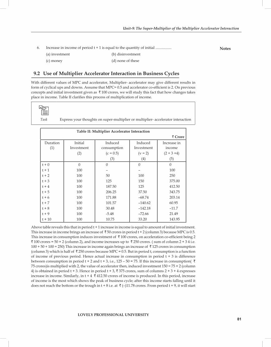
Increase in income of period t + 1 is equal to the quantity of initial ................. 6.

(a) investment (b) disinvestment

(c) money (d) none of these

Use of Multiplier Accelerator Interaction in Business Cycles.2

With different values of MPC and accelerator, Multiplier- accelerator may give different results in form of cyclical ups and downs. Assume that MPC= 0.5 and accelerator co-efficient is 2. On previous concepts and initial investment given as ` 100 crores, we will study this fact that how changes takes place in income. Table II clarifies this process of multiplication of income.

Task Express your thoughts on super-multiplier or multiplier- accelerator interaction

Table II: Multiplier Accelerator Interaction ` Crore

Duration (1)

Initial Investment

(2)

Induced consumption

(c = 0.5)(3)

Induced Investment

(v = 2)(4)

Increase in income

(2 + 3 +4)(5)

t + 0t + 1t + 2t + 3t + 4t + 5t + 6t + 7t + 8t + 9t + 10

0100100100100100100100100100100

0–50125187.50206.25171.88101.5730.48-5.4810.75

0–10015012537.50–68.74–140.62–142.18–72.6633.20

0100250375.00412.50343.75203.1460.95–11.721.49143.95

Above table reveals this that in period t + 1 increase in income is equal to amount of initial investment. This increase in income brings an increase of ̀ 50 crores in period t + 2 (column 3) because MPC is 0.5. This increase in consumption induces investment of ` 100 crores, on acceleration co-efficient being 2 ` 100 crores = 50 × 2 (column 2), and income increases up to ` 250 crores. ( sum of column 2 + 3 4 i.e. 100 + 50 + 100 = 250) This increase in income again brings an increase of ` 125 crores in consumption (column 3) which is half of ̀ 250 crores because MPC = 0.5. But in period t, consumption is a function of income of previous period. Hence actual increase in consumption in period t + 3 is difference between consumption in period t + 2 and t + 3, i.e., 125 – 50 = 75. If this increase in consumption( ` 75 crores)is multiplied with 2, the value of accelerator then, induced investment 150 = 75 × 2 (column 4) is obtained in period t + 3. Hence in period t + 3, ` 375 crores, sum of columns 2 + 3 + 4 expresses increase in income. Similarly, in t + 4 ` 412.50 crores of income is produced. In this period, increase of income is the most which shows the peak of business cycle; after this income starts falling until it does not reach the bottom or the trough in t + 8 i.e. at ` (–)11.78 crores. From period t + 9, it will start

Unit- : The Super-Multiplier of the Multiplier Accelerator Interaction

Notes


rising again which represent the phase of revival of the business cycle. This behaviour of income of first rising , then falling and then increasing at a fixed rate shows the mixed working of accelerator and multiplier. But actual behaviour of business cycle depends on the value of multiplier and accelerator as has been expressed by Samuelson in his Model.

Self AssessmentState whether the following statement are True or False:

Super multiplier has been calculated by adding both -the induced consumption and induced 7. investment.Super multiplier tells that if any initial increase happens in autonomous investment, then an 8. increase of Ks times of autonomous investment in income will take place.In period t + 2, in 100 income of t + 1 induced investment of 50 does not happen.9. Actual behaviour of business cycle depends on the value of multiplier and accelerator as has 10. been expressed by Samuelson in his Model.

Summary.3 In this relation Dr. Kurihara has targeted that marginal consumption tendency less than a �unit provides answer to this question that before complete collapse or in the situation of full employment why does accumulative process stop? According to Hanson, its reason is this that a big part of increase in income in each period is not spent on consumption in each next period. Through it there is a reduction in amount of internally induced investment and when such reduction increases by increase in induced consumption, then fall in income starts. In this manner, Prof Hanson has written, “It is marginal tendency of the saving only that stops the expansion process even then when at the peak of multiplier process through the process of accelerator expansion is increased.”

Keywords.4 Multiplier- Co-efficient. �Interaction- Process of meeting. �

Review Questions.5 Define super multiplier or multiplier- accelerator interaction.1. Mention “uses of multiplier- accelerator interaction In business cycles.”2.

Answers: Self Assessment1. Leverage Effect 2. low 3. (a) 4. (a) 5. (b) 6. (a) 7. True 8. True 9. False 10. True

Further Readings.6

Books Macroeconomics—1. Mohan Srivastava, DND publications, 2010.

Notes



82

Unit-10: Kaldor’s Theory of Trade Cycle Contents

ContentsObjectivesIntroduction10.1 Kaldor’s Theory of Trade Cycle10.2 Stabilisation Policies or Measures to Control Trade Cycles10.3 Summary10.4 KeyWords10.5 Review Questions10.6 Further Readings

Objectives


Know the Kaldor’s Theory of Trade Cycle, �

Know the Stabilisation Policies. �

Introduction

In form of a measure to control business ups and downs monetary policy is run by the central bank of a country. Central bank adopts many measures to control the quantity and quality of credit. For increasing the reserve of commercial banks it reduces rank rates and interest rates of the banks. It purchases securities from the open market. It reduces limit requirements on loans and motivates the banks to provide more loans to consumers, businessmen, traders etc.

Kaldor’s Theory of Trade Cycle10.1

Nicholas Kaldor constructed a model of trade cycle on the basis of Keynesian terminology of savings and investment. According to him it is the effect of cycle pressures that which takes the planned saving and investment of the economy towards equality. Actually, difference in planned saving and investment brings cycle. But cycle is possible only when saving and investments are non-linear.

Consider figure 10.1(A) and (B) where I and S are equal at the income level Y0 of equilibrium. But each situation is a situation of single balance. In the part A of the figure beyond Y0 where I > S is a situation of unstable imbalance because such situation will bring unlimited expansion, full employment and hyper-inflation. At the other side if S > I then such situation brings collapse along because of the downward movement towards the Figure .1


Notes


Hitesh Jhanji, Lovely Professional University

83

left side of Y0 as has been shown in part B of the figure. Kaldor leaves the functions of linear savings and investments because they are incapable of creating cycle. Instead of these he adapts non-linear savings and investments.

Notes Nicholas Kaldor constructed a model of trade cycle on the basis of Keynesian terminology of savings and investment.

A non linear investment function I has been shown in figure 26.2. As economy moves towards expansion phase, which has been shown by a left side movement along with curve I, where curve I is almost flat. It means that there is unused capacity at least level of others and net investment is there. But zero expansion starts then negative impact of accumulated capital is stronger on investment decisions in comparison to that on the high levels of production and profits. Opposed to it at high level of income when economy enters contraction phase the curve I again become flat and net investment reduces because increase in costs, increasing costs and increase in difficulties to take loan will prevent producers from expanding much faster. By this rate of increase in production reduces. It means that present capital stock and capacity is more than current production. This situation further reduces investment. Hence there is a fall in income and economy enters the phase of contraction by accumulative impact.

Did You Know? Kaldor shows the expansion of his trade cycle in three phases.

Similarly non linear savings function is shown in figure 26.3. At very low level of income, saving becomes very less. It may be negative also. In this way during the phase of expansion MPS is more. At general levels of income, increase in savings happen at lesser rate. It has been shown by the medium part of curve S. But at a very high level of income saving will be much and people will save a large part of their income.

Cycle can be seen only when none linear saving and investment curves are brought together as in figure 26.4. Figures A, B and C show multi-balances on situations. Of these A and B are stable conditions and C is an unstable condition. I > S between situations C and B below condition A, it will raise the level of income higher. S > I between conditions A and C and above condition B; it will lower the level of income.

But situations A and B are stable only in short term. In long term these conditions become unstable and path of the cycle is visible. For it Kaldor has used capital stock in form of another variable which has an impact on the relations of savings and investments. He took both, investments and savings in form of function of income and capital stock so that

Figure 26.2

Figure 26.3

Notes



84

S = f (Y, K)

I = f (Y, K)

dS dS0, 0IY dKdI dI0, 0dY dK

> >

> <

And, dI dSdY dY

>

In other words, in contraction phase, MPI > MPS

The above relations show that S and I directly change positively with Y. S changes directly with K and Y changes inversely with K.

Relation MPI > MPS shows the stability of the economy which takes it to either expansion or contraction. According to conditions 26.4, conditions A and B are ‘switch points’. These are those points at which, in long term, economies change their directions towards either expansion or contraction. Point C is unstable towards both the directions. When points B and C come closer the expansion phase of the cycle starts. When they meet then, expansion ends and contraction starts. Opposite to it when points C and A come closer then contraction starts. When they meet then contraction ends, and expansion starts.


Difference in planned saving and investment brings ..............1.

The Cycle is .............. of pressures.2.

Expansion Phase

Kaldor shows the expansion phase of his cycle in three stages. As in figure 10.5 stage 1, on starting from condition Y0 which is similar to figure 10.4. Assume that economy is in equilibrium at point C, but it is a point of unstable balance. C’s upwards movement shows that I > S, which takes the economy towards expansion path. Since investment rate is high, that is why capital stock of the economy increases at a sharp rate. But by increase of capital stock, marginal productivity of capital reduces and investment cycle shifts downwards. At the same time when there is an increase in capital stock of the economy it increases the income of the

Figure .4

Figure .5

Unit- : Kaldor’s Theory of Trade Cycle Contents

Notes


economy by which its savings increase. Hence savings curve shifts upwards. In the same way by the investment curve I shifting downwards and by savings curve S shifting upwards, point C comes closer to point B as has been shown in stage 2 of the figure 10.5. This process of curve I shifting downwards and curve S shifting upwards goes on until both curves do not touch each other and point C and point B do not meet as has been shown in stage 3 of the figure.10.5. But in this condition S > I in both directions, that is why in downwards direction it is an unstable condition. It takes the economy downwards until point A is not reached in stage 3.

Contraction PhaseContraction phase of trade cycle is also shown in three stages as in figure 26.6. Let us start from situation Y1 which matches with the point A in figure 10.4. It is the point of short term fixed balance but of a very low level of income. But at such low level of income, due to unused capacity in long term, capital stock reduces and investment curve I shifts upwards. Along with it savings reduce which shifts the savings curve downwards. Like this by curve I shifting upwards and curve S shifting downwards conditions A and C come close as has been shown in stage 5 of the figure. This process will go on slowly unless curves I and S dot not touch each other and conditions A and C do not meet as has been shown in stage 6 of figure 10.6. But at income level Y1 this condition of A + C is unstable in upwards direction because I I>S, it will take in expansive direction until economy does not reach at the high level of income Y2 at point B. From point B, curve I and S will slowly reach stage 1 shown in figure 10.5 and cyclical process starts again. In this way, Kaldor’s cyclical process is self-generating.

According to Kaldor, those forces which bring turn point towards bottom they are not definite at the high level. Boom will definitely end by itself. But depression may fall in static condition and may stay there until external changes (like discovery of new inventions, opening of new markets etc) do not come in its protection.

Then in Kaldor’s model, cycles are not necessarily of same length and duration and neither is expansion and contraction requisitely uniform. In reality, it depends upon slopes of curves I and S and by what rate do they shift in each stage of the cycle.

Kaldor in describing his theory of trade cycle uses neither acceleration rule nor monetary factors. Also he shows that how is trade cycle obtained without any growth factor.

Self AssessmentMultiple choice Question:

Cycles are possible only when savings and investments are ............... 3.

(a) non linear (b) linear

(c) more (d) less

Kaldor leaves the functions of linear savings and investments because they are ........................ 4. of creating cycle.

(a) incapable (b) capable

(c) ahead (d) behind

Figure .6

Notes



86

Difference in planned saving and investment brings .............. .5.

(a) deficit (b) cycle

(c) instability (d) none of these

Cycle can be seen only when none linear saving and investment curves are brought 6. ...................

(a) together (b) separately

(c) detached (d) none of these

Stabilisation Policies or Measures to Control Trade Cycles.2

For controlling the ups and downs in the economy many measures and suggestions are employed from time to time. Their objective is to stabilize economic activity for saving from ill-effects of boom and recession. For it below mentioned three measures are adopted.

1. Monetary Policy

In form of a measure to control business ups and downs monetary policy is run by the central bank of a country. Central bank adopts many measures to control the quantity and quality of credit. During boom, for controlling the expansion of money supply it increase bank rate, sells securities in open market, increases reserve ratio and adopts many selective credit control measures like increasing limit requirements, and regulating consumer credit etc. hence bank adopts expensive monetary policy. Taking loan by business and trades becomes expensive, difficult and selective. In this manner, efforts are made to control more quantity of money supply in the economy.

For control recession or depression, central bank adopts cheap or easy monetary policy. For increasing the reserve of commercial banks, it reduces bank rates and interest rates of the banks. He buys securities from the open market. It reduces limit requirements on loans and motivates the banks for giving loans to consumers, businessmen, traders etc.

Limitations of Monetary Policy

But monetary policy is not very effective in controlling boom or depression. If boom is due to cost push factors then it will not be effective in controlling inflation, total demand, production income and employment. As far as depression is related, experience of the great depression of 1930 tells that when there is pessimism in traders then success of monetary policy does not happen at all. In such situation they do not have at all the tendency to take loan, even if interest rates are very less. In this way, when there is reduction in income of which consumers and which are unemployed they reduce their consumption expenses. In such situation neither central bank nor commercial banks can motivate the consumers to increase total demand. In this manner success of monetary policy is very limited in controlling economic ups and downs.

2. Fiscal Policy

Monetary policy alone does not have the capacity to control trade cycle. That is why it is added to compensatory Fiscal policy. In born fiscal measures are very effective in controlling excessive government expenditure, personal consumption expenditure and personal and public investment. At the other side during depression they are helpful in increasing government expenditure, personal consumption expenditure and personal and public investment.

Unit- : Kaldor’s Theory of Trade Cycle Contents

Notes


Policy during Boom

Following measures are adopted during boom. For reducing demand for goods and services government cut down unnecessary expenses on non-developmental activities. In it there is a ban on personal expenses also, which depends on government demand for goods and services. But cutting down government expenditure is difficult. Then it is not possible to differentiate between necessary and unnecessary government expenditure. That is by this measure is completed by karaadhan. For reducing personal expense, government increases rates of personal company and goods taxes. When income is more than government expenditure then government adopts the policy of surplus budget. It may be done by either increasing tax rates or by reducing government expenditure or by both. It reduces income and total demand through opposite reaction of multiplier.

Another fiscal policy which is often adopted is taking loan from the public, effect of which is to reduce money with the public. Then repayment of public debt should be done and when economy stabilizes then payment should be postponed till any future date.

Task Express your thoughts about Kolder’s theory of trade cycle.

Policy during Depression

During depression government increases public expenditure and reduces taxes and adopts the policy of deficit financing. These measures increase total demand, production, income, employment and prices. Encrease in public expenditure increases total demand for goods and services and brings an increase in income through multiplier. Public expenditures are done on roads, drains, dams, parks, schools, hospitals and other construction works. They create demand for labour and personal construction industries and are helpful in reviving them. For inducing demand for consumer goods industries government also increases its expenditure on measures like unemployment insurance and social security. For deficit financing, loan taking by the government and idle money lying with financial institutions are used in investment plans.

Conclusion

Effectiveness of each cyclical fiscal policy depends on applying the policy work at right time and nature, quantity and organisation of public construction works.

3. Direct Controls

Objective of direct controls is correct allocation of resources for price stability. They are for influencing the important points of the economy. They influence special consumers and producers. They are in form of rationing, licensing, price and wage controls, export tax, exchange control, quota, monopoly control etc. They are more influential for removing obstacles and shortcomings created by inflationary pressures. But their success depends upon a skilled and loyal government, else black marketing, corruption, long queues and speculation may arise from them. Hence they must be used only during crisis like war, bad crops, hyper inflation etc.

Notes



88

ConclusionOf many measure of stabilisation policy any single method is not sufficient for controlling cyclical ups and downs. That is why all measures should be used together. Applying monetary policy is easy but it is less effective, because in capitalist system using cyclical policy and direct control is difficult but they are more effective. Because in capitalistic system, cyclical ups and downs are existent, hence it is not possible to end them completely. Some ups and downs may be good for economic growth and others not needed. Stabilisation policy should control unnecessary ups and downs.


Contraction phase of trade cycle is shown in three stages.7. According to Kaldor, those forces which bring turn point towards bottom they are not 8. definite at the high level.When there is an increase in capital stock of the economy it decreases the income of the 9. economyMonetary policy is more effective in controlling boom or depression.10.

Summary10.3 For reducing personal expense, government increases rates of personal company and goods �taxes. When income is more than government expenditure then government adopts the policy of surplus budget. It may be done by either increasing tax rates or by reducing government expenditure or by both. It reduces income and total demand through opposite reaction of multiplier.

Keywords10.4 Trade cycles—Business cycles. �Single—Only. �

Review Questions10.5 What is Kaldor’s trade cycle theory? Explain.1. Tell the stabilisation policies or measures to control trade cycles.2.

Answers: Self Assessment1. cycle 2. effect 3. (a) 4. (a)5. (b) 6. (a) 7. True 8. True

9. False 10. False


Books Macroeconomics: Theory and Policy—1. H.L Ahuja, S.Chand and Publishers, 2010

Macroeconomics: 2. S.K Chakravarty- Himalaya Publishing House, 2010.


Notes


Unit-11: Monetary Policy

ContentsObjectivesIntroduction11.1 Meaning of Monetary Policy11.2 Objectives and Goals of Monetary Policy11.3 Instruments of Monetary Policy11.4 Expansionary Monetary Policy11.5 Restrictive Monetary Policy11.6 Role of Monetary Policy in a Developing Economy11.7 Fiscal Policy11.8 Summary11.9 Keywords11.10 Review Questions11.11 Further Readings

Objectives


Know the meaning of monetary policy, �

Know the objectives of monetary policy, �

Know the expansionary monetary policy, �

Know the restrictive monetary policy. �

Introduction

Monetary policy is related to credit control measures adopted by the central bank. Is of two types: (1) Quantitative-general and indirect control; and (2) Qualitative. – selective or direct control. Under first category changes in bank rates, operations of open markets and changeable reserve requirements are included. Their objective is to regulate complete level of credit in the economy through the medium of commercial banks. In it changeable limit requirements and regulation of consumer credit are included.

Meaning of Monetary Policy11.1

By monetary policy is meant credit control measures adopted by the central bank of a country. Johnson defines monetary policy like this, “this policy is in the form of a tool to control the supply of money by the central bank with for achieving the objectives of general economic policies.”G.K Sha has defined it as “Any conscious activity done by monetary officer for changing quantity, availability or cost of money”

Notes


Hitesh Jhanji, Lovely Professional UniversityAdvance Macroeconomic Theory

90

Objectives and Goals of Monetary Policy11.2

Main objectives of monetary policy are as follows:

Full Employment: 1. Full employment has been kept under the main objectives of monetary policy. It is an important objective because by unemployment not only there is a loss of possible production but by it social prestige and self respect is also hurt. Apart from this it creates poverty. That is why attaining full employment is extremely important.

Notes Monetary policy is in the form of a tool to control the supply of money by the central bank with for achieving the objectives of general economic policies.

Price Stability: 2. Bringing stability in price level is one of the main objectives of monetary Policy.

Economic Growth: 3. In the recent years one of the most important objectives of monetary policy had been that there should be a fast economic development of the economy.

Balance of Payments: 4. Since the decade of 1950 another objective of monetary policy had been to maintain a balance of payment.


Full employment has been kept under the main ............ of monetary policy.1.

When prices start rising and there is a need to stop them then central bank sells .............. 2.

Instruments of Monetary Policy11.3

Monetary policy is related to credit control measures adopted by the central bank. Is of two types: (1) Quantitative-general and indirect control; and (2) Qualitative. – selective or direct control. Under first category changes in bank rates, operations of open markets and changeable reserve requirements are included. Their objective is to regulate complete level of credit in the economy through the medium of commercial banks. In it changeable limit requirements and regulation of consumer credit are included.

Bank Rate Policy:1. Bank rate is that minimum rate of loan giving by the central bank at which it re-discounts the first category hundies of exchanges and government securities adopted by the commercial banks. When central bank sees that inflationary pressures have started showing in the economy, it increases bank rates. Taking loan from central bank becomes expensive and commercial banks will comparatively take fewer loans from it. Commercial banks will increase their rate to giving loans to traders. That is why those taking loans will take fewer loans from commercial banks. Contraction of credit takes place and prices stop from rising further. As opposed to it when prices fall, then central bank reduces its bank rate. It is cheaper of commercial banks to take loan from central bank, and then commercial banks also reduce their rate of lending. By it traders are motivated to take more loans. Investment is induced. Production, employment, income and demand start to increase and prise stop falling.


Notes


Open Market Operations: 2. Open market operations are related to sale purchase of securities by the central bank in money market. When prices start rising and there is a need to stop them then central bank sells securities. Reserves of commercial banks reduce and they are not left in the situation to give loans to traders’ class. Further investment is discouraged and increase of prices stops. Opposed to it, when forces of recession start in the economy, then central bank purchases securities. Reserves of commercial banks increase. They give more loans, investment, production, employment and demand increases and falling of prices stops.

Changes in Reserve Ratios:3. Keynes had suggested this tool in his book Treatise of Money and United States of America was the first country which adopted it form of a monetary method. According to law each bank has to keep some percentage of its deposit in its godown in reserve and some percentage with the central bank. When prices start rising then central bank increases the reserve ratio. Banks have to keep more amounts with the central bank. Their reserves reduce and they give fewer loans. Unfavourable effect is there on the quantity of investment, production and employment. In situation opposite to it, when reserve ratio is reduced, then reserves of commercial banks increase. They give more loans and there is a favourable effect on the economic activity.

Selective Credit Controls: 4. Selective credit controls are brought in use to control special type of credit with specific objectives. For controlling speculative activities inside the economy these often take the form of changing margin requirements. When in economy or in specific areas, there is fast speculative activity in some goods and prices start to rise then central banks raise margin requirements on them. Result is this that those taking loan are given less money in form of loan on specific securities. For e.g. meaning of increasing margin requirement to 60 percent is that to the pledger of securities worth ` 10,000, 40 percent of its value (` 4000) will be given as loan. In situation of recession in specific fields, central bank by reducing margin requirements encourages loan acceptances.

Conclusion

For an effective analytic monetary policy it is important that bank rate, open market operations, reserve ratio and selective credit control measures are adopted together. But all monetary theorists have accepted that (i) in depression when trade confidence is at its weakest state, then success of monetary policy is zero; and (ii) it is successful against inflation. Monetarists say that in comparison to fiscal policies, monetary policies have more flexibility. They may be applied soon.

Did You Know? By monetary policy is meant credit control measures adopted by the central bank of a country.

Expansionary Monetary Policy.4

Expansionary (or cheap) monetary policy is used to come out of the deflationary gap or recession. When there is a decline in consumer demand of goods and services and trade demand for investment goods then deflationary gaps emerge. Central banks start expansionary monetary policy which makes the conditions of credit markets easy and brings an upward change in the entire demand.

For this objective central bank purchases government securities from open market, reduces reserve requirements of member banks, reduces discount rates and through selective credit measures

Notes



92

encourages consumer and trade credit. Through these measures it reduces the cost and availability of credit in the money market and improves the economy.

Expansionary monetary policy has been described through figure 11.1 (A) and (B). where initial recession is at R, Y, P, Q. In part (A) of the figure economy in already at extra money supply are interest rate OR. Consider that due to the credit policy of the central bank there is an increase in money supply in the economy. It shifts the curve LM rightwards to LM1. It increases the income from OY to OY1 and entire demand increases and in part (B) curve D shifts upwards to D1. Along with increase in demand for goods and services, production at high price level OP1 rises from OQ to OQ1. If expansionary monetary policy works properly then balance at point E1 may take place at full employment. But because of the below mentioned limitations possibility of reaching to that situation is not there.

Its Scope and Limitations

During the decades of 1930 and 1940 it was believed that in comparison to controlling boom and inflation, success of monetary policy was very limited in inducing recovery in depression. This concept emerged from the experiences of the great depression and publishing of the general theory of the Keynes.

Monetarists’ opinion is that during depression central bank through cheap credit policy may increase the reserves of the commercial banks. It may do so by purchasing securities or by decreasing the interest rates. As a result by increasing the facilities of those taking loans, banks’ capacity will increase. But experience of the great depression tells that during sharp depression when traders are pessimistic, then practically success of such policy is zero. In such situation banks are helpless on bringing revival. Since trade activities are almost in the situation of stagnancy hence traders have no tendency for taking loans to make inventories, though interest rates are very less. Since they want to reduce their already taken loans for inventories by returning. Apart from this question of taking loans for long term requirements does not arise in depression, when trade activity is already at very low level. With consumers also the condition is same who are struggling with reduced income and unemployment. Hence they do not wish to purchase any durable goods through bank loans. In this manner all banks may make credit available but they cannot compel traders and consumers to accept it. In the decade of 1930, very low interest rates and unused reserve amount with banks could have any important impact on world’s economies with depression.

“It is not said that during sharp contract cheap monetary policy will with without any profitable impact, but its most effect will be in preventing a bad situation from reaching to a worst situation. But restrictive monetary policy associated with downturn business will definitely make downturn business worse- its traditional example was the monetary policy of 1931 which gave its contribution in making the great depression serious…. At the other side if credit is easily available at favourable terms then definitely it will have a stabilising effect. It may become slow on fulfilment of liquidity requirements of the trade and perhaps may decrease the limit of downturn.”

But what was the cause of collapse of monetary policy in the decades of 1930 and 1940? Apart from painful and disillusion experiences during the great depression and after it, General Theory of Keynes

Figure .1

Unit- : Monetary Policy

Notes


in form of a tool for more stability became the causes of collapse of monetary policy. Keynes told that more flexibility liquidity preference schedule (liquidity net) presents monetary policy in form of helpless at the time of sharp depression.


Bringing stability in price level is one of the ................ of monetary policy.3.

(a) main objectives (b) main work

(c) plan (d) none of these

Attaining full employment is................. 4.

(a) important (c) extremely important

(c) main work (d) none of these

.................... are brought in use to control special type of credit with specific objectives.5.

(a) selective credit controls (b) objective

(c) specific areas (d) none of these

Central banks start expansionary monetary policy which makes the conditions of credit 6. markets...............

(a) difficult (b) easy

(c) changeable (d) none of these

Restrictive Monetary Policy.5

Monetary policy made for reducing the entire demand is known by the name of restrictive (or expensive) monetary policy. It is used to come out of an inflationary gap. Due to increase of consumer demand for goods and services, inflationary pressures are created in the economy and because of it boom also comes in trade investment. By increasing the cost and availability of bank credit for reducing entire consumption and investment central bank starts restrictive monetary policy. Central bank may do so by selling government securities in the open market, by increasing the reserve requirements of member banks, by increasing the discount rates and by controlling the consumer and trade credit through selective measures. Through these measures central bank increases the cost and availability of credit in the open market and by which it controls the inflationary pressure.

Its Scope and Limitations

But field of inflation in monetary policy is very limited in inflation control. Its limitations are as follows:

Increase in Velocity of Money:1. There is an important limit of effectiveness of monetary policy in stopping inflation- increase in velocity of money kept with the public. Central bank, through expensive monetary policy, may control money supply and cost of money but it has no such power by which it may stop the velocity of money. public may effectively bring in use money supply available with it as a result of which restrictive monetary policy becomes unsuccessful. It may be done in many ways.

Commercial Banks Portfolio Adjustment:a. When restrictive monetary policy is on, then commercial banks fulfil the demands of borrowers for loans by selling government securities to the central

Notes



94

bank. Such type of policy just changes the deposits kept by the banks in form of securities to active deposits. Government securities kept in the portfolio of the banks are substituted in place of loans. But there is no change in total deposit and money supply of the bank. But through it, total expense increases, because banks lend money to borrowers. In this manner restrictive monetary policy of the central bank becomes ineffective.

Then, when banks sell government securities to central bank, their prices fall in the market and rate of interest on them increases by it general interest rate structure in the market increases. But by fall of prices of securities banks will have capital losses and banks will not like to suffer those. It depends on it that whether banks hope that fall in securities prices (or increase in interest rates) is short term or is going to last long. If banks hope that decline in security prices will stay for some time only then instead of selling those (securities) at capital loss, they will like to keep them. At the other side if they hope that decline in securities prices will go on for some time then for giving loans to the customers at high rates they will sell the securities and will fulfil the capital- loss by sale of securities by giving the loans at high interest rates. But once demand for loans will reduce then banks will be able to buy back the government securities at prices lower than that at which they had sold them and will again be in profit in this deal. In this way, commercial banks’ policy of portfolio adjustments increases the velocity of net money despite an expensive monetary policy and as a result expensive monetary policy is left ineffective.

Role of non-Banking financial Intermediaries:b. NBFIs stop the money supply controlling capacity of monetary policy in two ways. First, they sell securities for giving loans and like commercial banks, increase the velocity of money in the same way as has been described above. Secondly, under expensive monetary policy as the rate of interest increases on securities, in order to achieve more reserves from the savers financial intermediaries keep increasing interest rates of deposits with them. It encourages savers that they give their inactive money to these intermediaries by which their loan capacity increases further. In this way these intermediaries are successful in increasing the velocity of money as a result of which expensive credit policy is left incapable.

Methods to make better use of available money supply:c. Many methods have been devised for better use of available money supply which makes restrictive monetary policy ineffective. Some such methods are there like development of better methods of fund collection of sales financial institutions; in comparison to commercial banks more loan taken by NBFI from the public etc. By obtaining funds from various sources of commercial banks, such institutions, even under restrictive monetary policy, are successful in increasing the velocity of available supply of money.

Discriminatory:2. Expensive monetary policy has discriminatory influence on various fields of economy. It is said that those firms which depend on internal sources under financial system, they are not influenced by restrictive monetary policy. At the other side, only those firms are influenced which depend on banking system for funds. Especially it is understood in relation to expensive monetary policy that it works against the traders, because they are extremely sensitive towards changes in credit costs reason for which is that they cannot take credit risk and are ageist residential construction and some types of state and local government expenditure. It can not only slow their expenditure but may even stop it.

Threat to Credit Market: 3. If central bank strictly controls credit market and investors expect interest rates to rise continuously then it may end loan sum reserves of credit market. Consequently securities may not be sold and credit market may stop working.

Threat to solvency of NBFIs:4. Strong restrictive monetary policy, through fast increasing interest rates, may create a threat to solvency of savings banks and savings and loan


Notes


institutions like NBFIs. This happens because different from commercial banks, they are not in a conditions to keep themselves balanced in fast increasing interest rates.

Changes of Expectations of Borrowers and Lenders:5. A very expensive monetary policy may change the expectations of borrowers and lenders. That is why they bring unchangeable changes in credit market situations. Sharp increase in interest rates changes the expectations so much that when this policy is given up and an expansionary monetary policy is started, even then lender are unwilling to give long term loans with an anticipation of further increase in interest rates. At the other side, borrowers, with an anticipation of increase in interest rates in future, may take long term loans though they do not need it.

Time Lags: 6. One more limitation on effectiveness of expensive monetary policy is that there are time lags in need for action and identification, decision and popularization of action. Since due to these time lags monetary officers are not able to follow measures of restrictive monetary policy on time that is why monetary policy works very slowly. Hence it is not very effective in controlling inflation.

Self AssessmentState whether the following statements are true or false:

Monetarists have the opinion that central bank may increase the reserves of commercial 7. banks during depression, through cheap monetary policy.

Full employment is not kept under the main objectives of monetary policy.8.

There is an important limit of effectiveness of monetary policy in stopping inflation—increase 9. in velocity of money kept with the public.

When banks sell governments securities to central banks, their price in the market rise up. 10.

Role of Monetary Policy in a Developing Economy.6

In a developing economy, monetary policy does an important job in increasing economic growth by influencing cost and sufficiency of credit, by controlling the inflation and maintaining the equilibrium of balance of payment. Hence in such countries main objectives of monetary policy is to control credit, stabilise exchange rate for controlling inflation and for stabilising prices, attain equilibrium in balance of Payment and increase economic growth.

To Control Inflationary Pressures: 1. For attaining control on inflationary pressures created during the process of development, both quantitative and qualitative measure credit control of monetary policy are required. In tools of monetary policy, open market operations are not successful in controlling credit in undeveloped countries because bill market is small and undeveloped. Commercial banks keep flexible cash deposit ratio because they are not completely controlled by the central bank. Because of relatively low interest rate from them, they are unwilling to invest in government securities. Apart from this instead of investing in government securities they like to keep their reserves in liquid form like gold, foreign exchange and cash. Commercial banks also to not want to take loans or do re-discounting from central bank.

Bank rate policy is also not that effective in such countries because of the following reasons: - (i) shortage of discount bills; (ii) contracted shape of bill market; (iii) huge non-monetised field where goods exchange happens (iv) existence of local banks which do not do discounting of bills with central bank; (v) tendency of commercial banks of keeping large cash reserve; and (vi) being of large unorganised money market.

Notes



96

Use of Variable Reserve Ratio in form of a tool of monetary policy in LDCs is more effective in comparison to bank rate policy and open market operations. Since market of securities is very small hence open market operations are not successful. But increase or decrease in variable reserve ratio by the central bank increases or decreases cash available with commercial banks without having an unfavourable influence on prices of securities. Again, commercial banks keep huge cash reserves with cannot be reduced by the central bank. But by increasing variable reserve ratio, liquidity of banks is reduced. There are some limitations of use of variable reserve ratio in LDCs- first, since non-banking financial intermediaries do not keep deposits with central banks that is why they are not influence by it. Secondly, those banks which do not keep extra liquidity, in comparison to them, those who keep it are influenced more.

But in influencing the allocation of credit and consequently in influencing the procedure of investment qualitative measures of credit control are more effective in comparison to quantitative measures. In LDCS strong tendency is found to invest in gold, jewellery, inventories, tangible assets etc in comparison to optional productive sources available in agriculture, mining, plantation and industries. For controlling and limiting credit facilities for such unproductive objectives qualitative credit control is more appropriate. They are useful in limiting speculative activities in matter of larders and raw materials. They are more useful in stopping sectional inflation in the economy. They cut the demand for import by making it compulsory for importers to deposit advance amount equivalent of foreign exchange. It also has this influence that reserve rates of banks reduce so much so that in this process their deposits are transferred to the central bank. Selective credit control measures may be in form of change in limit requirement instead of definite type of security, consumer credit regulation and rationing of credit.

To Achieve Price Stability: 2. Monetary policy is an important tool to attain price stability. It brings appropriate adjustment in money demand and supply. Imbalance in both of these will be reflected in price level. Decrease in money supply stops growth, while it excess will bring inflation. When economy is marching towards development then by increase in agricultural and industrial production and by slowly changing of non-monetised areas to monetised areas, demand for money rises slowly. By it demand for money for exchange and speculation objectives will also increase. Hence monetary officer, for stabilising prices and stopping inflation, will have to increase supply of money more than the ratio of demand for money.

To Bridge BOP Deficit:3. In form of interest rate policy, monetary policy does a very important task for bridging the BOP deficit. For achieving the planned target of development developing economies have to face serious Balance of Payment difficulties. For establishing foundational structures like electricity, irrigation, transportation etc and for directly productive activities like iron and steel, fertilizers, chemical etc such countries have to import capital equipments, machinery, raw material, parts and furniture. Because of which there is an increase in their export. But their exports are stagnant and because of inflation prices of export are also very high. As a result difference in import and export is created because of which balance of payment is imbalanced. Monetary policy through high interest rates may be helpful in bridging the deficit of balance of payment. High interest rates are helpful in reducing the difference in balance of payment by motivating inflow of investment.

Interest Rate Policy: 4. For a developing economy high interest rate policy encourages more savings, develops banking habits and provides strength to monetization of the economy, which is necessary for capitalization and economic development. High interest rate policy also removes inflation because it discourages borrowing and investment of speculation and investment. Then this policy encourages allotment of scarce capital resources towards more productive sources. Some economists are supporter of low interest rates in such countries


Notes


because high interest rates are hurdle in development but experienced results tell this that in developing countries investment in trade and industry is interest-inflexible but in net cost of investment, interest has a very little ratio. Despite of these opposing opinions, it is correct for the monetary officer to follow discriminatory interest rate policy. According to this policy for high interest rates should be there for unnecessary and unproductive experiments and for productive experiments low interest rates should be there.

To Create Banki5. ng and Financial Institutions: In LDCs, one objective of monetary policy is to establish and develop banking and financial institutions for collecting, floating and inducing savings. Monetary officer should encourage establishment of branch banking in rural and urban areas. Such policy will be helpful in monetization of non-monetized area and will induce saving and investment for capital building. It will also organise and develop money and capital market. It is necessary of developmental monetary policy, in which debt management is also included.

Debt Management: In a developing country, managing public debt is one of the important tasks of monetary policy. Its objective is to issue government bonds on appropriate time, stabilising their prices and minimising the service costs of public debt. Main objective of debt management is to create such situations in which public debts keep increasing year on year. In such countries public debts are necessary for controlling money supply and providing finance to development programmes. But public debt should necessarily be at cheap rates. Low interest rates increase the price of government bonds and make them more attractive for the people. They also feel the weight of debt to be less.

Conclusion: In this way entire monetary policy, as has been told above, is helpful in controlling inflation, reducing the Balance of Payment gap, inducing capital building and in increasing the economic development.

Limitations of Monetary Policy in LDCs

Experience of developing countries tells that monetary policy has a limited role in such countries. Below mentioned are its reasons:

Large Non-Monetized Sector:1. In such countries there is large non monetized area which is a hurdle in success of monetary policy. Most of the people live in rural areas where there is a trend of goods exchange method. Consequently, monetary policy is unsuccessful in influencing a wide part of the economy.

Undeveloped Money and Capital Market:2. Money and capital markets are undeveloped. There is a lack of bills, stocks and shares which limit the success of monetary policy.

Large number of NBFIs:3. In such countries local bankers such as Non Banking Financial Intermediaries work on a large scale, but they do not come under the control of monetary officer. Because of this reason also effectiveness of monetary policy is limited in such countries.

High Liquidity:4. High liquidity is found with the commercial banks because of which they are in affected by the credit policy of the central bank. It also makes the monetary policy less effective.

Foreign Bank:5. Almost in all developing countries foreign commercial banks are there. They also by selling the foreign assets and by taking out money from their main office, make the monetary policy less effective, while central bank may be following expensive monetary policy.

Notes



98

Less Bank Money:6. In such countries monetary policy is also not successful because bank money is a small ratio of total money. As a result of which, central bank is incapable of controlling credit in an effective manner.

Money not Deposited with bank:7. Prosperous people do not deposit money with banks instead use them for jewellery, gold, real assets, speculative consumption etc. Such activities encourage inflationary pressures because they do not come under the control of monetary officer.

Task Express your thoughts in relation to expansionary monetary policy.

Fiscal Policy.7

1. MeaningBy fiscal policy is meant use of taxation or public expenditure by the government for stabilisation or growth. "By fiscal policy we refer to government actions affecting its receipts and expenditures which we ordinarily take as measured by the government’s net receipts, its surplus or deficit." Government may balance undesirable changes in personal expenses and investment by anti-cyclical changes in public expenditure and taxes. Arthur Smiths has defined fiscal policy like this, “A policy under which the government uses its expenditure and revenue programmes to produce desirable effects and avoid undesirable effects on the national income, production and employment. Though the last objective of fiscal policy is long term stabilisation of the economy, still this objective may be achieved only by taking care of economic ups and downs. In this context Otto Eckstein has defined fiscal policy like this, “Changes in taxes and expenditures which aim at short run goals of full employment and price-level stability."

2. Objectives of Fiscal Policy

Below mentioned are the objectives of Fiscal Policy:

To attain and maintain full employment,1.

To keep the price level stable,2.

To stabilize the growth rate of the economy,3.

To maintain balance in the Balance of Payment,4.

To increase the economic development of under developed countries. 5.

3. Instruments of Fiscal Policy

By the medium of change in government expenditure and taxation fiscal policy strongly influences national income, employment, production and prices. Increase in public expenditure during depression increase total demand for goods and services and does a huge growth in income by the way of multiplier process, while the influence of reduction in taxes is that disposable income increases as a result of which people’s consumption and investments increase. At the other side during inflation decrease in public expenditure decreases total demand, national income, employment, production and prices whereas increase in taxes reduces disposable income and consequently reduces consumption and


Notes


investment. In this way through a strategically combination of expenditure and taxation programmes government may control inflationary and deflationary pressures in the economy. Now we will discuss various sources of Fiscal policy-

Budgetary Policy:1. Contra Cyclical Fiscal Policy

Budget is an important source of fiscal policy. Budgetary policy controls the results and relations of receipts and expenditures of fiscal policies. Further we discuss those general budget policies, which are adopted for stabilising the economy:

Budget Deficit:(i) Fiscal Policy under Depression- Deficit budget is an important measure to control depression. When government expenditure exceeds its receipts then in the thread of national income more than that quantity is put in as much has been taken out from it. Deficit expresses net expenditure of the government which increase the national income multiplier times the net expenditure. If MPC is 2/3, multiplier will be 3 and if in government expenditure there is a net increase of ` 100 crores then it will increase the national income to ` 300 crores. In this way budget deficit puts an expansionary effect on total demand, even if by fiscal process marginal tendencies are unchanged and disposable receipts are redistributed. Expansionary effect of the budget has been shown in figure .1 in non-linear form. C is the consumption function. C + I + G expresses consumption, investment and government expenditure (total expenditure function) before the presentation of budget. Assume that government expenditure G is increased in the economy. Consequently, total expenditure function shifts upwards to reach C + I + G’. Income increases from OY to become OY1 where as equilibrium situation moves from E to E1. In comparison to increase in government expenditure E1B (= Δ G) increase in income YY1 + EA = E1A is more. BA (E1A – E1B) expresses increase in consumption. In this way budget deficit is always expansionary because as compared to amount of actual government expenditure there is more increase in national income. In this method of budget deficit taxes are kept as it is.

Budget deficit may be obtained by doing reduction in taxes and without reducing government expenditure. Reduction in taxes leaves comparatively more disposable income in hands of the people and in this way increased consumptions induce expenditure. As a result it further increases total demand, consumption income and employment. It has been clarified in figure

.2 where C is the original consumption function. Assume that quantity ET is reduced in taxes. By this consumption function will shift upwards and reach C’ and from OY income will increase to become OY1.

But reduction in taxes is not very expansionary from the path of increased consumption expenditure, because it may happen that tax relief is not spent on consumption and is saved. If business expectation are low then it may happen that traders may also not invest much. For saving from such dangers what government need to do is that he along with reduction in taxes also follows the policy of government expenditure. Its multiplier effect will be much more in that situation when we assume that because of tax relief some consumption and investments also increase.

Figure .2

Figure .3

Notes



100

Surplus Budget:(ii) Fiscal Policy Under Boom- There is a surplus in the budget when government expenditure exceeds the revenue. Policy of surplus budget is followed for controlling inflationary pressures inside the economy. It may happen by increase in taxation pr by decrease in government expenditure or by both. By it there will be a reduction in income and total demand, which (reduction) as a result of increased taxes will be equal to multiplier times of reduction in government and/or personal consumption expenditure. It may be made clear with the help of figure .1. where economy is in initial equilibrium condition at E1.

Assume that there is a reduction of amount of ΔG in government expenditure by which total expenditure function shifts downwards to C + I + G. When E is the new balance situation which tells that as a result of reduction of E1B in government expenditure income falls from OY1 to OY. Reduction in income Y1Y = AE > E1B which is the reduction in expenditure because in consumption also there is a reduction of BA.

When there is an increase in taxes then despite of government expenditure there may be surplus budget. Increased taxes reduce disposable income of the people and motivate reduction in consumption. Result is that there is a reduction in total demand, production, employment and income. It has been made clear in figure .3. Before levying tax, C is the consumption function. Assume that tax equivalent to ET is levied then consumption function will shift downwards to C1. New equilibrium condition is E1. Consequently income fall from OY to OY1.

Balanced Budget Multiplier:(iii) Another expansionary fiscal policy is Balanced Budget. In this policy, amount of increase in taxes and increase in government expenditure is the same. Its result is that net national income increases. Its reason is that reduction in consumption due to levying of tax is not equal to government expenditure.

2. Compensatory Fiscal Policy

Objective of compensatory fiscal policy is to compensate economy against unending trends towards inflation and deflation by adjusting public expenditure and taxes. That is why it becomes necessary for it that at any definite time instead of measures forever long term lasting fiscal measures are adopted. When there are deflationary trends in the economy then government must reduce its expenditure through deficit budget and reduction in taxes. Doing so is necessary for compensating reduction in personal investment and for increasing effective demand, employment, production and income inside the economy. At the other side, when inflationary trends are there, the government must reduce its expenditure by making a surplus budget and increasing taxes so that economy may be made stable at full employment level. There are two ways of compensatory fiscal policy: (i) Built-in Stabilisers and (ii) Discretionary Action

Built-in Stabilisers: 1. Meaning of built-in stabilisers is that without any plan from government’s side, adjustment of expenditures and taxes in the process of cyclical ups and downs inside the economy. Under this arrangement changes happen in the budget automatically that is why it is also called automatic technique of stabilization. Following are the various automatic stabilisers—incorporated profit tax, income tax, production tax, survivor and unemployment insurance and unemployment relief payment. In form of sources of automatic stabilisation tax and expenditure are related to national income. On unchanged structure of tax rate

Figure .4


Notes


being given, tax receipts, along with movements in national income, change directly, while government expenditure change inversely with changes in national income. When national income falls in downward phase of trade cycle, which is based on the percentage of national income, reduce them and as a result tax income reduces. Along with it, government expenditure on unemployment relief and social security benefits increase automatically. There will be an automatic loss in the budget which will stop deflationary trends. At the other side in the upwards phase of trade cycle when national income rises fast then on an increase in tax rates, tax receipts will increase automatically. Also government expenditure on unemployment relief and social security benefits will decrease on its own. These two forces will themselves build a surplus budget and in this way inflationary forces will be controlled themselves.

Merits

In form of fiscal measure, built-in stabilisers have many merits. First, when personal purchasing power falls then built-in stabilisers do the job of cushion for it and during deflationary conditions, they reduce the difficulties of the people. Second, they stop the national income and consumption level from falling at low level. Thirdly, in this measure budgetary changes are automatic and there is no delay in taking administrative decision. Fourth, automatic stabilisers minimise the wrong forecasts and mistakes of time of fiscal measures. Lastly, they unite the short term and long term fiscal policies.

Limitations

But in form of an automatic compensatory measure effectiveness of built-in stabiliser depends on the flexibility of tax receipts, level of taxes and on flexibility of public expenditure. As much more will be the flexibility of tax receipts that much more powerful will be automatic stabilisers in controlling inflationary and deflationary trends. But flexibility of tax receipts is not so much that even in developed countries like America they may do the job of automatic stabiliser; secondly when level of taxes is low then during downswing in form of automatic stabiliser high flexibility of tax receipts also do not have much importance. Thirdly, built-in stabilisers after giving tax do not think over the secondary effects of trade-income stabilisers and consumption expenditure on trade expectations. Fourthly, this measure is silent about the stabilisation effects of local bodies, state governments and personal fields of the economy. Fifth, they cannot end trade cycles, they can only reduce their intensity. Sixth, their effects are no favourable from recession to recovery. That is why, economists have suggested that from discretionary fiscal policy of fiscal policy, built in stabilisers are substituted (anupoorit).

3. Discretionary Fiscal Policy

For discretionary Fiscal policy there is need for bringing such thoughtful changes in the budget like changes in tax-rates or government expenditure or both. Generally it takes three forms. (i) change in taxes, when expenditure stays stable (ii) change in expenditure, when tax stays stable, (iii) change in tax and expenditure together.

First, when there is a deduction in taxes while no change is done in government expenditure, then there is an increase in disposable income of this business and domestic area. Personal expenditure increases by it. But increase in income depends on the fact in whose tax and to what extent deduction is done and do the tax payers consider this deduction as permanent or temporary. If those attaining profit from tax deduction are people of high middle income group then there will be an increase in total demand. If it is related to low income group then there will be not much increase in their total income. If traders have not motivation to invest, then tax deduction will not motivate them to invest.

Notes



102

At the end, if tax payers consider the tax reduction to be temporary then this policy will be less effective that is why this policy is more effective in controlling inflation by increasing taxes because by high rates of taxes there will be a reduction in disposable income of people and businessmen, by which there will be a reduction in total demand. Secondly, for controlling deflationary trends, second method is more useful. With taxes remaining unchanged, if government increases its expenditure on goods and services then total demand will increase equal to increase in government expenditure. At the other side if government expenditure is reduced during inflation then it in not much effective, because trader expectations of the economy are of high trade of which there is no possibility to reduce effective demand. Third method is much more effective and better than the other two methods of stop inflationary and deflationary trends. For stopping inflation, taxes must be increased and government expenditure reduced. At the other side for facing depression, taxes may be reduced and government expenditure may be increased.

Limitations

Discretionary fiscal policy depends on right time and correct forecast. First, correct forecast is necessary to know that stage of the cycle through which the economy is passing. Only then it is possible that complete fiscal activity may be done. Wrong forecast may instead of slowing the cyclical ups and downs, may increase it. Actually, for correct forecasting, economics is not a complete science. As a result, fiscal action is always taken when in the trade cycle, turn points have arrived. Secondly, there are two time lags of public fiscal policy. First is “decision lag”, which is related to the time that is taken in study of the problem and in taking the decision. Lag found in this process may be very long. Secondly, once the decision is taken then “application lag” is there. In it that expenditure is found which has been allocated for application of programme. In country like U.S.A, it may take more than two years and in a country like U.K., more than a year. Thirdly, some public plans are so complex that with an objective to increase or decrease expenditure on them, it is not possible to make them slow or fast.

Summary11.8

In comparison to change in tax rates because of higher multiplier effect of government �expenditure, in comparison to expenditure tax changes may be applied much faster. That is why for controlling cyclical ups and downs more emphasis is being laid on taxation in form of best fiscal measure. In this manner, when turn point of trade cycle is already on then discretionary fiscal policy gives power to built-in stabilisers, as is the experience of developed nations like USA.

Keywords11.9

Fiscal Policy—Financial policy. �

Goals— objectives. �

Review Questions11.10

What do you understand by Fiscal policy? Tell the difference between three main types of 1. discretionary fiscal policy.

Analyse compensatory Fiscal Policy.2.

Do a critical analysis of automatic stabilisation.3.


Notes


Answers: Self Assessment1. objectives 2. securities 3. (a) 4. (b)

5. (a) 6. (b) 7. True 8. False

9. True 10. False


Books Macroeconomics: Theory and Policy—1. H.L Ahuja, S. chand Publishers, 2010.

Macroeconomics—2. S.K Chakra Varty, Himalaya Publishing House, 2010.

Macroeconomics:3. Economic Growth, Fluctuations and Policies— Robert E. Hall and David H. Paipal, Vaina Books, 2010.

Notes



104

Unit-12: Mundell Model

ContentsObjectivesIntroduction12.1 Fiscal Monetary Policy for Internal and External Balance: The Mundellian Model12.2 Summary12.3 Keywords12.4 Review Questions12.5 Further Readings

Objectives


Know the objectives of Mundell, �

Know the criticisms of Mundell Model. �

Introduction

In the objective of external balance allotment of monetary policy and in the objective of internal balance, allotment of fiscal policy must be done. But allotment rule works only when monetary and fiscal policy without any long lag (pashchataa) are continuously and well accommodated, before their impacts become visual. This is the “Mundell rule” of successful use of monetary and fiscal policy for internal and external stability, as per which, an instrument must be combined with that target only on which it has the maximum relative influence. He calls it the Principle of Effective Market Classification.

Fiscal Monetary Policy for Internal and External Balance: The 12.1 Mundellian Model

Mundell has discussed about the relation between two instruments and two targets. Two instruments are monetary policy expressed through interest rate and fiscal policy expressed through the government expenditure. The two targets are full employment (internal balance) and balance of payment balance (external balance). Allotment rule is of monetary policy for the objective of external balance and for internal balance is doing of fiscal policy. Allotment of these instruments in the targets is shown in figure .1.

Notes Mundell has discussed about the relation between two instruments and two targets.


Notes


Hitesh Jhanji, Lovely Professional University

105

In the figure, horizontal axis measure the rate of interest (monetary policy) and vertical axis measures the savings budget (Fiscal Policy). FF is the internal balance line and XX is the external balance line. Line FF expresses full employment. Its slope is negative because for maintaining full employment cut in the savings budget has to be definitely balanced by increase in interest rate. Inflation is below this line FF (in Zone III and IV) and above it (Zone I and II) is recession. On the other side, line XX give all the points of balance in balance of payment. Its slope is also negative because by doing cutting savings budget imports increase, for stopping which it is necessary to improve capital account by increasing the interest rate. Below this line (in Zone I and IV) there is loss in balance of payment and above this line (in zone II and III), there is surplus. In comparison to line FF, slope of line XX is much straight because when interest rates increase for balancing the expanding fiscal Policy (increase in Budget deficit or cut in savings budget); it motivates an undercurrent flow of short term capital for external balance. Towards interest rate changes as much relative will be capital momentums that much more will be line FF and XX of straight slope. By this monetary policy become comparatively more effective in maintaining external balance.

Figure 12.1 shows the internal and external balance and tells that in maintaining balance between these two what job does monetary and fiscal policy do? Assume that in zone I, economy is at point A where there is full employment in the economy and deficit in balance of payment. For ending the deficit in balance of payment monetary officer first makes an increase of AB in interest rates so that the supply of money may be reduced. By reducing money supply demand for goods will decrease and by it imports will decrease further and at point B balance will be established at balance of payment. At this point there will be recession and unemployment in the economy. For correcting it and for bringing internal balance, reduction of the amount BC will have to be done, but at point C again there is loss in balance of payment, that is why it Is important that for reducing money supply, further increase of CD is done in interest rate. At point D, internal balance is again disturbed because of which there is further cut in savings budget. After decrease of money supply, by this process of decrease in savings, at the end economy reaches point E where there is internal and external balance simultaneously.


Monetary and fiscal policies ............... under definite practical constraint. 1.

Prescribed policy mix cannot be ............ in correcting the current account deficit.2.

At the other side, if for removing the deficit in balance of payment savings budget is brought in use and for ending unemployment and recession, monetary policy is adopted, then neither there will be internal balance nor external balance. If we move from point A then, by an increase in savings budget economy will move to K where though external balance is available, but there is unemployment

Figure 12.1

Notes



106

and recession in the economy. For removing it, interest rate is reduced by KL for increasing money supply. But at point L, in balance of payment, deficit increase from its previous level. For it still LM more savings budget will be necessary. For it, it will become necessary that further cut is made in the interest rates so that recession and unemployment are removed. Like this economy will keep moving farther from point E and internal and external balance will never happen together. In such situation allotment rule brings an explosive instability because policies have been coordinated badly.

Did You Know? Allotment rule is of monetary policy for the objective of external balance and for internal balance is doing of fiscal policy.

In this way in objective of external balance allotment monetary policy and in objective of internal balance, allotment of fiscal policy must be done. But allotment rule works only when monetary and fiscal policy without any long lag are continuously and well accommodated, before their impacts become visual. This is the “Mundell rule” of successful use of monetary and fiscal policy for internal and external stability, as per which, an instrument must be combined with that target only on which it has the maximum relative influence. He calls it the Principle of Effective Market Classification.

In reality, Mundell contends for a rational mix of monetary and Fiscal policy. In zone II and IV there is no disproportion in joint use of monetary and fiscal policy. In zone II both policies must be restrictive and in zone IV, both policies must be expansive. In rest of the two zones monetary and fiscal policies must be definitely mixed for achieving both the targets together. According to Mundell, when monetary policy is combined with objectives of external balance and Fiscal policy is combined with objective of internal balance, and then both the objectives are met.


In objective of external balance allotment of monetary policy and in objective of internal 3. balance allotment of ............. must be done

(a) Fiscal policy (b) Money

(c) Principles (d) None of these

In reality, Mundel ............... for a rational mix of monetary and Fiscal policy4.

(a) sophistry (b) contends

(c) meaning (d) none of these

Monetary-Fiscal mixture is not a true adjustment .............. 5.

(a) Mechanism (b) Payment

(b) Policy (d) Capital

When interest rate is increased by the medium of monetary policy then it brings ............. in 6. domestic investment.

(a) decline (b) increase

(c) stability (d) none of these


Notes


Criticism of Mundell’s Model

But there are some shortcomings of this analysis:

Unrealistic Assumptions:1. This model assumes that officers know the limit at which economy is far from both the internal and external balance so that appropriate monetary and fiscal policy may be used. This is also assumed beforehand that they know quantitative results which are possible by the use of each policy. But these assumption are far from reality, because it is not possible to correctly judge the category of imbalance. Hence changing the policy may not be appropriate for such imbalance.

Overlook of Unemployment and Inflation:2. This analysis overlooks unemployment and inflation. It is unreal, because this concept which is known by the name of stagflation is often found in all developed countries.

Neglect of other Factors:3. This analysis only thinks over difference in interest rates a reason for capital momentum and ignores other factors such as exchange rate changes. Other than this it is not possible that continuous deficit is financed by capital momentum.

Practical Constraints of Monetary and Fiscal Policies:4. Monetary and Fiscal policies work under a definite practical constrainte of political reasons, some governments are not able to follow restrictive fiscal policy and monetary policy with high interest rates. Though such policies may be started, but they cannot be successful, because capital flow cannot be interest sensitive.

Unsuccessful Prescribed Policy Mix:5. Prescribed policy mix cannot be successful in correcting current account deficit because policy mix influences both- capital flow and imports, which is why it only ensures that negative business balance is compensated by positive capital flow and also vice versa.

Task Expresses your thoughts in relation to the Mundel’s Model

Not True Adjustment Mechanism:6. Monetary-Fiscal mixture is not a true adjustment mechanism. It does not adjust balance of payment but only makes it stable. Capital flow, leaving the prices and income unchanged, only completes the gap between the sovereign demand and supply of foreign exchange.

No Consideration on the Debt Servicing Requirements:7. This analysis does not make consideration on Debt servicing Requirements because, when domestic interest rates are increased then, continuous capital flow will happen on the current account of balance of payment.

Decrease in investments at home:8. When interest rates are increased by the medium of monetary policy, it will bring a decrease in domestic investment. It should definitely be accompanied by either a decline in government expenditure or tax cut or by any composition of the two. Such monetary- fiscal policy mixture misuses the savings of the economy by turning them towards debt financed government expenditure, which stops capital building. According to Johnson, “It creates the problem of ‘ineptitude vs proficiency’ in use of domestic savings possibility”

Conflicts between Prescribed Policy Mixes:9. There is a possibility of inter conflict between the prescribed policy mixes of governments of various countries. Johnson has told, “In all countries together reach the right combination of monetary and fiscal policies, particularly

Notes



108

if adjustment of policies is done by examination and defects relating to order, then it will be a complex process and under some circumstances instead of taking in the direction of balance, it may take far from it."


In the objective of external balance allotment of monetary policy and in the objective of 7. internal balance allotment of fiscal policy must be done.It is possible to finance continuous deficit by capital momentum.8. Prescribed policy mixture cannot be successful in correcting current account deficit.9. There is a possibility of inter conflict between the prescribed policy mixes of governments 10. of various countries.

Summary12.2 In reality, Mundell contends for a rational mix of monetary and Fiscal policy. In zone II and �IV there is no disproportion in joint use of monetary and fiscal policy. In zone II both policies must be restrictive and in zone IV, both policies must be expansive. In rest of the two zones monetary and fiscal policies must be definitely mixed for achieving both the targets together. According to Mundell, when monetary policy is combined with objectives of external balance and Fiscal policy is combined with objective of internal balance, and then both the objectives are met.

Keywords12.3 Surplus—Excess. �Conflict—Internal struggle. �

Review Questions12.4 What do you understand by “Mundell’s Model”?1. Describe Fiscal Monetary policy for internal and external balance.2.

Answers: Self Assessment1. work 2. successful 3. (a) 4. (b)5. (a) 6. (a) 7. True 8.False9. True 10. True

Further Re12.5 adings

Books Macroeconomics: Theory and Policy—1. H.L Ahuja, S. Chand Publisher, 2010

Macroeconomics: Economic Growth, Fluctuations and Policy—2. Robert E. Hall and David H. Paipal, Vaina books, 2010.

Macroeconomics—3. S.K. Chakravarty, Himalaya Publishing House, 2010.


Notes


Unit-13: Swan Model

ContentsObjectivesIntroduction13.1 Policies for Internal and External Balance: Expenditure Switching and Expenditure

Reducing13.2 Summary13.3 Keywords13.4 Review Questions13.5 Further Readings

Objectives


Know the policies for internal and external balance, �

Know the expenditure switching and expenditure reducing. �

Introduction

Monetary fiscal policies have definite objectives which may be obtained by use of policy equipment. These are- full employment, economic progress, price stability, and equilibrium of balance of payment. These objectives are often mutually opposing. Monetary and Fiscal policies study about nature of these oppositions and about the appropriate resources between them or about establishing inter-relation between them. Analysis of these problems has centred mainly around internal and external objectives. Internal balance is related to income and full employment and external balance is related to the equilibrium of balance of payment.

Theory of economic (monetary or fiscal) policy has centred around two separate problems. First, relation between number of policy objectives and number of policy equipments; and second, allotment of policy equipments for achieving the objectives.

John Tinbergen was the first economist who had said that number of policy equipments should be equal to number of objectives. If as compared to policy equipments, numbers of objectives are more then, it means that requisite tools are not there for fulfilment of policy objectives. At the other side, if as compared to number of objectives, numbers of policy equipments are more then it means that there is not one composition by which problem will be solved, not who knows how many combinations are there. In this manner, it is important for the success of economic policy that number of policy equipments is equal to number of objectives. It came to be known as Tinbergen rule or fixed target approach.

The second problem arises that when number of policy equipments and policy objectives is same then, how the equipments should be allotted among the targets for achieving the given objectives. In the absence of coordination,correct value of objectives can be achieved by the rendering of distribution problem.

Notes


Ashwani Panesar, Lovely Professional UniversityAdvance Macroeconomic Theory

110

Notes Monetary fiscal policies have definite objectives which may be obtained by use of policy equipments.

Policies for Internal and External balance: Expenditure Switching and Expenditure Reducing

Johnson only has pointed towards policy equipments for bringing both internal and external balance. He named them expenditure reducing or internal policy and expenditure switching or external policy.

Deficit in balance of payment means excess of expenditure over income. For correcting it, similarity should be brought in income and expenditure. Objective of expenditure reducing policies is to reduce all demand by the medium of more taxes and interest rates, by which expense and production reduces. Further, fall in income and expenditure reduces domestic price level. By this there is a change in expenditure on domestic goods from foreign goods. As a result imports of the country reduce. Objective of expenditure switching policies is to increase the demand for domestic goods and to switch the expenditure from imported goods to domestic goods. Such expenditure switching increases domestic production. Until the extreme tendency of spending is less than the unit, it will improve the equilibrium of payment balance of the country.

For simultaneously achieving objectives of both internal and external, a judicious combination of expenditure reducing and expenditure switching equipments is necessary. For e.g. if economy is at full employment level then because of the policy of devaluation there may be inflation in the economy. That is why for maintaining balance of payment equilibrium and full employment along with the expenditure switching policy of devaluation, there must be more expenditure reducing policies of monetary and fiscal control.

Relat ion between pol icy equipments for simultaneously obtaining both objectives of internal and external balance has been analysed in form of Trevor–Swan model as described in figure 13.1.


Fall in Production and expenditure reduces ______ price level.1.

Deficit in balance of payment means excess of ______ over income.2.

The Swan Model

Swan investigates appropriate combinations of expenditure reducing and expenditure switching policies for achieving internal and external balance.

Figure 13.1

Unit-13: Swan Model

Notes


Did You Know? Deficit in balance of payment means excess of expenditure over income.

Assumptions

This model is based on these assumptions that (a) Trade restrictions do not exist (b) capitalist do not exist and; (c) productivity, terms of trade and other financial transfers are given. In figure 13.1, horizontal axis measures the real domestic expenditure and vertical axis expresses the cost ratio which is the indicator of relative costs and shoes the competitiveness of the economy. Any movement towards left (towards 0) on the horizontal axis means use of expenditure reducing policy and any upward movement on vertical axis means use of expenditure switching policy. FF is the internal balance curve which expresses the situation of full employment. It shows various combinations of cost ratio and real domestic expense. A given level of employment can be obtained by either a level lower than a very favourable relative form of cost ratio and domestic expenditure or by a level upper than a less favourable relative form of cost ratio and domestic expenditure. In this way curve FF bends towards the right. Clearly, part towards the right of curve FF (upper) is related to inflation of situation of more than full employment and part towards the left of curve (lower) expresses recession or unemployment.


Objective of expenditure reducing policies is to ............ all demand by the medium of more 3. taxes and interest rates

(a) reduce (b) add

(c) increase (d) none of these

it is important for the success of economic policy that number of policy equipments is equal 4. to ..............

(a) number of policy objectives (b) objectives

(c) policy (d) equipments

If economy is at full employment level then because of the policy of devaluation there may 5. be ............ in the economy.

(a) deflation (b) inflation

(c) loss (d) decrease

Theory of economic (monetary or fiscal) policy has ........... around two separate problems.6.

(a) collected (a) centred

(c) discreet (d) none of these.

Curve XX shows the external balance where in lack of capitalists, export is equal to import. That is why, external balance happens when net exports become zero. This curve grows from left to right side which means that for economy to stay in external balance should definitely equilibrium devaluation by increase in domestic expenditure. (Devaluation, by encouraging export and discouraging import will improve the trade balance of the country and increase in real domestic expense will increase the import of the country in sufficient quantity). Clearly, part above the curve XX is related to saving and the part below it shows the deficit of balance of payment.

Notes



112

That point where curve FF intersects the curve XX, expresses the Bliss point, where economy is in internal and external balance simultaneously. In figure 13.1 E is such a point, where there exchange rate and real domestic expenditure are in balanced. If economy is not at point E, then it is in imbalance. According to Swan, “Both curves of internal balance and external balance divide the situation in four zones of economic misfortune.” Four zones of imbalance are:-

Zone I: Inflation and payment balance surplus

Zone II: Unemployment and payment balance surplus

Zone III: Unemployment and payment balance deficit

Zone IV: Inflation and payment balance deficit.

Task Express your thoughts about internal and external balance policies.

Policy Measures

For description of types of policy measures, which are important for simultaneously obtaining internal and external balance, we will take it in eight possible condition of imbalance in figure 13.2. For these conditions, various combinations of policy measure are important.

Many countries are in equilibrium at point A of curve XX in payment balance and unemployment (or recession). For such situation there is need for extension of domestic economy through increase in domestic expense. It will reduce net exports. For making this tendency ineffective devaluation should be added to increase in domestic expenditure.

If deficit moves along in unemployment and payment balance, as happens in Zone III at point K, then there should be an increase in domestic expenditure. Policies increasing Internd demand by the medium of expansive measures also increase domestic employment. But this policy increases the deficit in balance of payment. It is described in form of “dilemma zone” because instead of expansive policy, devaluation is preferred policy.

In balance of payment, if economy adds full employment with deficit, as happened at point D of curve FF, the devaluation is its only solution. This huge pre-defined will create surplus and extra foreign demand will bring inflation in domestic economy. For stopping these tendencies, little devaluation will have to be added to cut in domestic expenditure.

Take point H in Zone IV where domestic inflation is added to deficit in balance of payment. Inflation should be stopped by a cut in domestic expenditure which will also reduce deficit in balance of payment and finally will take the economy towards balanced situation E.

If there is equilibrium of balance of payment and inflation as on point B then it should increase its rate of exchange and reduce the domestic expenditure.

Figure 13.2

Unit-13: Swan Model

Notes


Take point G in Zone I where surplus in balance of payment is added to inflation. In such situation, for correcting the surplus of balance of payment, exchange rate should be increased and for stopping inflation expenditure should be reduced. But cut in exchange rate will increase the surplus. It again expresses the “Dilemma Zone.”

If the country in the situation of full employment and excess in balance of payment at point C of curve FF then it should increase its rate of exchange. But increase in rate of exchange will create unemployment. In order to be saved from it, domestic expense must be increased.

At the end, let’s move to point F of Zone II where surplus in balance of payment is added to unemployment. Here increase in domestic expenditure will be appropriate for both, internal and external balance. Such policy will increase employment and for reducing the size of surplus, will also induce increase in import.

Above mentioned analysis presents this that if economy is neither at curve FF (internal balance) nor at XX curve (external balance), then it is in any one of the four zones.

When for achieving one objective (say, internal balance ), economy follows only one policy or both expenditure switching and reducing domestic expenditure policies together, then it moves from the other objective(say, external balance ). This problem arises not only in “Dilemma zones” I and III but also in “uncomplicated areas” II and IV. For example, if we take point F in Zone II where surplus in balance of payment is added to unemployment, then expansive policy will reduce unemployment and will also reduce surplus. But for taking the economy to full equilibrium point E then, price increase or price decrease exchange rate will have to be accepted which will remove the economy from one objective or other objective.


Policies increasing Internal demand by the medium of expansive measures also increase 7. domestic employment.

External balance happens when net exports become zero.8.

Both curves of internal balance and external balance divide the situation in four zones of 9. economic misfortune.

Deficit in balance of payment means deficit of expenditure over income.10.

Summary13.1

Theory of economic (monetary or fiscal) policy has centred around two separate problems. �First, relation between number of policy objectives and number of policy equipments; and second, allotment of policy equipments for achieving the objectives.

Keywords.2

External balance—Outer balance. �

Internal balance—Balance of inside. �

Notes



114

Review Questions.3

What did Johnson do to bring both, internal and external balance?1.

What is Swan Model? Clarify. 2.

Answers: Self Assessment1. domestic 2. expenditure 3. (a) 4. (a)

5. (b) 6. (b) 7. True 8. True

9. True 10. False

Further Readings.4

Books Macroeconomics: Theory and Policy—1. H.L Ahuja, S. Chand Publisher, 2010.

Unit- : Swan Model

Notes


Unit-14: Rational Expectations Hypothesis

ContentsObjectivesIntroduction14.1 Adaptive Expectations14.2 Rational Expectations14.3 Basic Propositions of Rational Expectations Hypothesis14.4 Stabilisation Policy and Ratex Hypothesis14.5 Summary14.6 Keywords14.7 Review Questions14.8 Further Readings

Objectives


Know the Adaptive Expectations, �

Know the Rational Expectations, �

Know the Stabilisation Policy and Ratex Hypothesis. �

Introduction

In the decade of 1930, when Keynes wrote his “General Theory”, then the main problem of the world was unemployment. During the Second World War, inflation emerged in form of the main economic problem. After the world war, unemployment again emerged as a problem till the decade of 1960. Till next one century, unemployment and inflation jointly took a new form, which was called stagflation. This new problem of stagflation became a challenge before the policy makers and economists, because this theory of Keynes was silent on this subject. Hence a new macroeconomic theory was born by this crisis situation which was named “Rational Expectations Hypothesis OR Ratex”.

Adaptive Expectations14.1

Before discussing about the Ratex hypothesis, it is important to understand the meaning of adaptive expectations used in macroeconomics which was developed before the Ratex theory.

Expectations are forecast or predictions made by any financial agent in relation to those uncertain economic factors which are related to his decisions. Forecasts, along with the tendencies of the past, are based on current information and experience. Main part of economic theory, in development of expectations by the financial agents (i.e., consumers, producers etc.) is based on assumption of their rational behaviour. But till now economists, in measurement of human behaviour, have not been able to include the role of expectations. Keynes discussed the importance of expectations but he was silent on the fact that how are they developed?

Notes


Ashwani Panesar, Lovely Professional UniversityAdvance Macroeconomic Theory

116

Notes Thought of rational hypothesis was first presented by John Mooth in 1961, who had taken this thought from engineering literature.

In recent years economists in model development have made an extensive use of adaptive expectation hypothesis. In this relation work done by Cagen in 1956 and by Nerlove in 1957 was very important. According to adaptive expectations hypothesis, it is the expectation of the financial agents that future will also definitely be like the tendencies of the past. They expect future prices of economic variables like price income in form of average of their past prices and the change in them to be in a very slow speed. Financial agents make the expected prices of these variables equal to the weighted average of their past and present prices. They change their expectations according to previous forecast errors. Errors that took place as a result of previous behaviours point towards an important source of information for development of hypothesis. But such expectations are based on these assumptions that financial agents expect very little change to take place on those mistakes. Hence when there are changes in economic policy then often meaningless forecasts happen through it.

For example, according to adaptive expectation hypothesis, financial agents develop the expectations of future inflation rate by the weighted average of the average inflation rates experienced earlier and if actual inflation is about to be different from expected inflation then they revise those expectations from time to time. It expresses the irrational behaviour of financial agents. Freidman’s analysis of long-term Philips curve is based on adaptive expectation hypothesis. Assumption hidden in acceleration hypothesis of Friedman that price expectations are primarily based on experience of previous inflation is unrealistic. When price expectations of the financial agents are based on this assumption then they are irrational. If they think so in situation of rising prices, they will find themselves to be wrong. Its reason is that development of hypothesis is done not only by previous projections but by direct forecasts of future also. Basis of people’s expectations is previous price changes along with present information in relation to many factors. In this manner, rational people for forecasting the inflation of the future with more reality, make use of all available information.

Self AssessmentFill in the Blanks:

When there are changes in economic policy then often meaningless ............ happen through 1. it.

Ratex Hypothesis is applied to ................ policy. 2.

Rational Expectations14.2

Thought of rational expectations was first presented by John Mooth in 1961, who had taken this thought from engineering literature. His model is about modelling price activities of the main market. If we move with the assumption that financial agents, at the time of developing expectations, make the skilled and most desired use of information, then they create such theory of expectations by which reaction of consumers and producers on expected price changes depends on their reaction on actual price changes. Mooth’s saying is that some expectations are rational in these meanings and that incidents are different only because of some random mistake only.

Mooth’s imagination of rational expectations is related to microeconomics. Many economists were not satisfied by it. Hence it remained inactive for ten years. During the beginning of the decade of 1970,


Notes


Robert Lucas, Thomas Sargent and Neil Wallace used this thought for the problems of macroeconomics policies.

Did You Know? Mooth’s imagination of rational expectations is related to microeconomics.

Basic Propositions of Rational Expectations Hypothesis14.3

Ratex hypothesis believes that financial agents by using all economic information available with them, build expectations of future prices of economic variable like prices, income etc. This information specially incorporates in itself relations related to economic variables like monetary and fiscal policies of the government. In this way, those building expectations believe that financial agents have complete and correct information about the events of the future. According to Mooth information should be considered like any other rare resource. Apart from this, rational financial agents while making their expectations should make use of the knowledge related to economic system. Hence Hypothesis of Ratex believes this that personal financial agents use complete available information in building expectations and they prepare this information from their rational. This assumption is important that Ratex does not express the consumer or firm to be far sighted or their expectations to be always correct. It indicates that agents think over the previous errors and if necessary, to stop the reoccurrence of such errors, review their expected behaviour. Objectively such assumptions indicate that agents are successful in removing regular expected errors so that such errors are average unrelated to available information.

Ratex hypothesis may be applied to economic (monetary, fiscal and income) policies. Those applying rational expectations have shown ineffectiveness of stabilising policies. According to them, due to change in economic policies (monetary, fiscal and income), no one has much information about the effects of it on the economy. Specially, it means to put a stop on Macroeconomic policies as tax cutting, increasing government expenditure, increasing money supply or making a deficit budget etc for controlling economic recession. Their reasoning is that public has learnt this from the previous experience that government will follow such policies. That is why government by adapting these influences cannot befool the public and mere indication of such policy may create expectation of countercyclical reaction from the government. In this way according to Ratex hypothesis people make assumptions about fiscal and monetary policies of the government and while taking financial decisions, pay attention towards them. As a result of it, by the time indications about governmental policies are received, public had already worked upon them and their impact ends. In other words, Ratex Hypothesis tells this that policy-moves bring changes in the financial behaviour of the people which are not expected beforehand and they are unexpected moves from the government. Once when people receive information about the policy and there is expectation of its getting started then it may bring changes in the financial behaviour of the people.

Rational Expectations and the Phillips Curve

In the acceleration hypothesis of Phillips curve promoted by Friedman, short term trade-off between unemployment and inflation but long-term trade-off is not there. It reason is that inflationary expectations are based on previous tendency of inflation which cannot be forecasted exactly correct. Because the expected rate of inflation is always behind its actual rate, which is why an observed error is found. For adjusting the expected rate of inflation with its actual rate, by adding some ratio

Notes



118

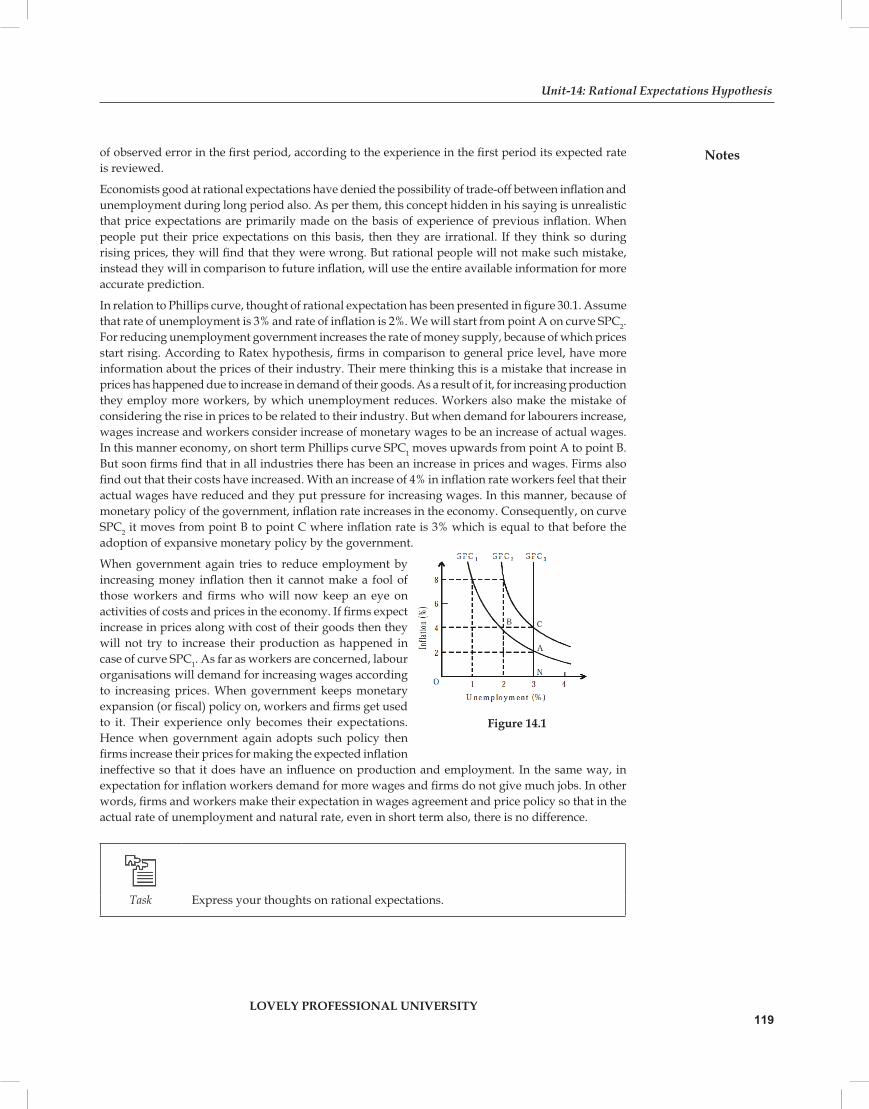
of observed error in the first period, according to the experience in the first period its expected rate is reviewed.

Economists good at rational expectations have denied the possibility of trade-off between inflation and unemployment during long period also. As per them, this concept hidden in his saying is unrealistic that price expectations are primarily made on the basis of experience of previous inflation. When people put their price expectations on this basis, then they are irrational. If they think so during rising prices, they will find that they were wrong. But rational people will not make such mistake, instead they will in comparison to future inflation, will use the entire available information for more accurate prediction.

In relation to Phillips curve, thought of rational expectation has been presented in figure 30.1. Assume that rate of unemployment is 3% and rate of inflation is 2%. We will start from point A on curve SPC2. For reducing unemployment government increases the rate of money supply, because of which prices start rising. According to Ratex hypothesis, firms in comparison to general price level, have more information about the prices of their industry. Their mere thinking this is a mistake that increase in prices has happened due to increase in demand of their goods. As a result of it, for increasing production they employ more workers, by which unemployment reduces. Workers also make the mistake of considering the rise in prices to be related to their industry. But when demand for labourers increase, wages increase and workers consider increase of monetary wages to be an increase of actual wages. In this manner economy, on short term Phillips curve SPC1 moves upwards from point A to point B. But soon firms find that in all industries there has been an increase in prices and wages. Firms also find out that their costs have increased. With an increase of 4% in inflation rate workers feel that their actual wages have reduced and they put pressure for increasing wages. In this manner, because of monetary policy of the government, inflation rate increases in the economy. Consequently, on curve SPC2 it moves from point B to point C where inflation rate is 3% which is equal to that before the adoption of expansive monetary policy by the government.

When government again tries to reduce employment by increasing money inflation then it cannot make a fool of those workers and firms who will now keep an eye on activities of costs and prices in the economy. If firms expect increase in prices along with cost of their goods then they will not try to increase their production as happened in case of curve SPC1. As far as workers are concerned, labour organisations will demand for increasing wages according to increasing prices. When government keeps monetary expansion (or fiscal) policy on, workers and firms get used to it. Their experience only becomes their expectations. Hence when government again adopts such policy then firms increase their prices for making the expected inflation ineffective so that it does have an influence on production and employment. In the same way, in expectation for inflation workers demand for more wages and firms do not give much jobs. In other words, firms and workers make their expectation in wages agreement and price policy so that in the actual rate of unemployment and natural rate, even in short term also, there is no difference.

Task Express your thoughts on rational expectations.

Figure 14.1


Notes



Before discussing about the Ratex hypothesis, it is __________ to understand the meaning 3. of adaptive expectations used in macroeconomics.

(a) important (b) unimportant

(c) sufficient (d) none of these

In the decade of 1930, when Keynes wrote his “General Theory”, then the main problem of 4. the world was _______.

(a) employment (b) unemployment

(c) labour (d) capital

During the Second World War, inflation emerged in __________.5.

(a) form of the main economic problem (b) form of war

(c) form of peace (d) none of these

Forecasts, along with the tendencies of the past, are based on current information and 6. ________.

(a) news (b) experience

(c) theory (d) rules

Stabilisation Policy and Ratex Hypothesis14.4

According to Ratex hypothesis monetary and fiscal (stabilization) policies are ineffective in short term, because correctly guessing the expectation in short term is not possible. It is called policy impotence. Ratex hypothesis is bases on this assumption that industries and firms keep correct information about forthcoming economic activities. That is why their expectations are rational because they are based on all available information, especially government activities. If government follows any favourable monetary or fiscal policy then people know about it and according to it only they adjust their plans. Hence whenever government adopts any possible policy then it is not effective because people by predicting it had already adjusted their policies according to it. It means that government policy is ineffective. Another important assumption is that all markets are completely competitive and wages are completely flexible.

Come; first let’s take fiscal policy only. Those followers of theory of Keynes, advocate for an active fiscal policy for reducing unemployment. But according to Ratex hypothesis cut in tax and/or increase in government expense will reduce unemployment only if its short term effects on the economy are unexpected for the people In other words, a fiscal policy may have a short term effect for reducing unemployment, if people do not have a pre-assumption that prices will increase. But whenever government sticks to such policy, then people have the hope for increase in inflation rate. Hence in inflation workers seeing the possibility of heavy increase will demand for more wages and firms predicting a rise in future costs will increase the prices of their goods. As a result of it fiscal policy will be ineffective in short term. Through it, in long term, unemployment and inflation may increase, when government tries to control inflation.

Similarly if government for reducing unemployment, increases money supply through an expansive monetary policy, then it will also be ineffective in short term. Such policy may reduce unemployment in short term only if its influence on the economy is not predicted. But when government sticks to such expansive monetary policy then people have an expectation of increase in inflation rate. Firms increase prices of their goods by which possible inflation may be made inactive so that it does not

Notes



120

have any influence on production. Similarly, predicting an increase in inflation workers demands for more wages and firms do not give employment to more workers. Hence it has no influence on unemployment.

If seen in this way, Ratex hypothesis suggests this that expansive fiscal and monetary policies will have a temporary impact in unemployment and if continued, may increase inflation and unemployment. Success of such policies is only when people may not forecast them. Once when people forecast them and mould themselves according to it then economy returns to its old natural rate of unemployment. Hence for short term impact of fiscal and monetary policies on unemployment, government will have to fool the public. But it does not happen always. If government continues these policies then they become ineffective because it is difficult to befool people for a long time and they forecast its effects on production and unemployment. In this way, fiscal-monetary policies become ineffective in short term. According to those supporting Ratex hypothesis, inflation cannot be controlled without doing extensive unemployment, if government declares monetary and fiscal policies and instead of surprising people, explain them about it.

CriticismsEconomists have criticised Ratex hypothesis on the following basis:

Unrealistic Assumptions:1. Assumption of rational expectation is unrealistic. Critics reason is that big firms may predict correctly but small firms and general workers will not be able to do so.

Costly Information: 2. Collecting information, its analysis and broadcasting is very expensive. Hence there is no appropriate market for information. That is why most financial agents cannot work on the basis of rational expectation.

Different Information:3. Critics also believe that information available to the government is different from the information received by the firms and workers. Accordingly, expectation of firms and workers regarding the possible rates of inflation may not necessarily be different realistic rates just because of random error. But government on the basis of available information may correctly predict the difference between the possible and expected rate of inflation.

Prices and Wages not Flexible:4. Though reach of government and people to the information is equal, still there is no guarantee that their expectations will be rational. Critics say that prices and wages are not flexible. Economists like Phillips, Taylor and Fisher have shown this that if prices and wages are stable then monetary and fiscal policies may be effective even in short term. Meaning of stability of wage rates is they adjust with the market powers in a comparatively slower form because wage contracts are applicable for two-three years at a time. In the same way, from the beginning of the period possible price level is expected to be maintained till the end of the time period. Hence if expectations are rational also, monetary and fiscal policies may impact production and unemployment in short term.

Expectations Adaptive:5. Gordon has completely rejected the reason of Ratex hypothesis. He has told two reasons- First, any person does not keep sufficient knowledge for predicting the level of market adjusted prices and sticks to adaptive expectations. Second, even if any how he learns about the structure of the economy still rational expectations will be very near to adaptive expectations.

Government not Impotent:6. It is often said that according to Ratex Hypothesis, government is incapable in economic field. But Ratex economists do not believe this, but their faith is that government has a deep impact on economic policies.


Notes



Those followers of theory of Keynes, advocate for an active fiscal policy for reducing 7. unemployment.

Similarly if government for reducing unemployment, increases money supply through an 8. expansive monetary policy, then it will also be ineffective in short term.

It is the faith of Ratex’s economists that government does not have a deep impact on economic 9. policies.

Gordon has completely rejected the reason of Ratex hypothesis.10.

Summary14.5

Mooth’s imagination of rational expectations is related to microeconomics. Many economists �were not satisfied by it. Hence it remained inactive for ten years. During the beginning of the decade of 1970, Robert Lucas, Thomas Sargent and Neil Wallace used this thought for the problems of macroeconomics policies.

Keywords14.6

Stagflation—Speed-less inflation. �

Past—Previous. �

Review Questions14.7

What are adaptive expectations? Describe.1.

Describe rational expectations.2.

Comment of ‘Stabilisation policy' and 'Ratex hypothesis.3.

Answers: Self Assessment1. forecasts 2. economic policies 3. (a) 4. (b)

5. (a) 6. (b) 7. True 8. True

9. False 10. True


Books Macroeconomics— 1. S.K. Chakravarty, Himalaya Publishing House, 2010.

Macroeconomics:2. Economic Growth, Fluctuations and Policies— Robert E. Hall and David H. Paipal, Vaina Books, 2010.

Notes



122

"%7"/$& MACROECONOMIC THEORY

Documents

Transcript of "%7"/$& MACROECONOMIC THEORY