www.elsevier.com/locate/ijforecast

International Journal of Forec

Business and consumer expectations

and macroeconomic forecasts

Oscar Claveria *, Ernest Pons 1, Raul Ramos 2

Grup d’Analisi Quantitativa Regional (AQR), Espai de Recerca en Economia,

Facultat de Ciencies Economiques i Empresarials, Universitat de Barcelona, Avda. Diagonal 690-08034 Barcelona, Espanya

Abstract

Business and consumer surveys have become an essential tool for gathering information about different economic variables.

While the fast availability of the results and the wide range of variables covered have made them very useful for monitoring the

current state of the economy, there is no consensus on their usefulness for forecasting macroeconomic developments.

The objective of this paper is to analyse the possibility of improving forecasts for selected macroeconomic variables for the

euro area using the information provided by these surveys. After analyzing the potential presence of seasonality and the issue of

quantification, we tested whether these indicators provide useful information for improving forecasts of the macroeconomic

variables. With this aim, different sets of models have been considered (AR, ARIMA, SETAR, Markov switching regime

models and VAR) to obtain forecasts for the selected macroeconomic variables. Then, information from surveys has been

considered for forecasting these variables in the context of the following models: autoregressive, VAR, Markov switching

regime and leading indicator models. In all cases, the root mean square error (RMSE) has been computed for different forecast

horizons.

The comparison of the forecasting performance of the two sets of models permits us to conclude that, in most cases, models

that include information from the surveys have lower RMSEs than the best model without survey information. However, this

reduction is only significant in a limited number of cases. In this sense, the results obtained extend the results of previous

research that has included information from business and consumer surveys to explain the behaviour of macroeconomic

variables, but are not conclusive about its role.

D 2006 International Institute of Forecasters. Published by Elsevier B.V. All rights reserved.

JEL classification: C53; C42

Keywords: Macroeconomic forecasts; Forecast competition; Business and consumer surveys

0169-2070/$

doi:10.1016/

* Correspo

E-mail ad1 Tel.: +342 Tel.: +34

asting 23 (2007) 47–69

- see front matter D 2006 International Institute of Forecasters. Published by Elsevier B.V. All rights reserved.

j.ijforecast.2006.04.004

nding author. Tel.: +34 93 4021012, +34 93 4021825; fax: +34 93 4021821.

dresses: oclaveria@ub.edu (O. Claveria), epons@ub.edu (E. Pons), rramos@ub.edu (R. Ramos).

93 4021412; fax: +34 93 4021821.

93 4021984; fax: +34 93 4021821.

O. Claveria et al. / International Journal of Forecasting 23 (2007) 47–6948

1. Introduction and objectives

Business and consumer surveys have become an

essential tool for gathering information about different

economic variables. While the fast availability of the

results and the wide range of variables covered make

them very useful for monitoring the current state of

the economy, there is no consensus on their usefulness

for forecasting macroeconomic developments.

The objective of the paper is to analyse the

possibility of improving the forecasts for some

selected macroeconomic variables for the euro area

using the information provided by business and

consumer surveys. As pointed out by Pesaran

(1987), this type of data is less likely to be susceptible

to sampling and measurement errors than surveys that

require respondents to give point forecasts for the

variables in question. One might think that the

information provided by qualitative indicators could

be useful for improving forecasts of quantitative

variables for two reasons. First, statistical information

from business and consumer surveys is available

much earlier than quantitative statistics; and second,

these indicators are usually related to agents’ expect-

ations, so they are likely to be related to future

developments of macroeconomic variables.

In this paper, we have considered all the

information available for the business and consumer

survey indicators in the euro area. The data set

analysed includes 38 indicators (33 of which are

monthly and 5 quarterly) and 6 composite indicators.

Although the starting date of these indicators differs,

most of them begin in January 1985 (or in the first

quarter of 1985). The latest period to be included in

the analysis is December 2005 (or the last quarter of

2005).3 More details on the data set can be found in

Table 1.

The strategy to test whether these indicators

provide useful information to improve forecasts of

the macroeconomic variables is the following.

First, macroeconomic variables that could be

related to the information provided by business and

consumer surveys have been selected and statistical

3 Data used in this paper was obtained from the European Commis-

sion DG ECFIN website http://europa.eu.int/comm/economy_finance/

indicators/business_consumer_surveys/bcsseries_en.htm) in March

2006.

information for the longest time-span available has

been collected from the Eurostat and ECB databases.4

Tables 2 and 3 show more details about this data set of

macroeconomic variables and the correspondence

between the business and consumer survey indicators

and these macroeconomic variables.

Second, five different sets of models have been

considered (AR, ARIMA, self-exciting threshold

autoregression [SETAR], Markov switching regime

and vector autoregression models [VAR]) to obtain

forecasts for the different quantitative variables, and

the root mean square error (RMSE) and the mean

absolute percentual error (MAPE) have been comput-

ed for different forecast horizons. The comparison of

these values with the ones obtained with models

where information from business and consumer

surveys has been considered would permit to assess

whether these indicators improve the forecasts or not.

Third, information from surveys is considered for

forecasting the quantitative variables using three

different types of models:

(i) Lagged selected indicators are introduced as

explanatory variables in autoregressive and

VAR models. For Markov switching regime

models, the probability of changing regime

depends on the information of the qualitative

indicators rather than on the own evolution of

the series.

(ii) Leading indicator models are constructed for

each of the quantitative variables using infor-

mation from business and consumer survey

indicators.

(iii) One problem with survey data is that, in contrast

to other statistical series, their results are

weighted percentages of respondents expecting

an economic variable to increase, decrease or

remain constant. Therefore, the information

refers to the direction of change but not to its

magnitude. This is the reason why we think that

the considered list of qualitative indicators

should be previously quantified in order to

obtain more reliable forecasts of businessmen’s

opinions. The conversion of qualitative data into

4 Data used in this paper was obtained from the Eurostat website

(http://europa.eu.int/comm/eurostat) and the ECB website (http://

www.ecb.int) in March 2006.

Table 1

List of business and consumer surveys indicators for the Euro area

Code Description Frequency Sample Observations Categories

v1 Economic Sentiment Indicator Month jan-85 dec-05 252

v2 Industrial Confidence Indicator

(v7+v4�v6)/3

Month jan-85 dec-05 252

v3 Production trend observed in

recent months

Month jan-85 dec-05 252 p e m b

v4 Assessment of order-book levels Month jan-85 dec-05 252 p e m b

v5 Assessment of export order-book levels Month jan-85 dec-05 252 p e m b

v6 Assessment of stocks of finished products Month jan-85 dec-05 252 p e m b

v7 Production expectations for the months ahead Month jan-85 dec-05 252 p e m b

v8 Selling price expectations for the months ahead Month jan-85 dec-05 252 p e m b

v9 Employment expectations for the months ahead Month jan-85 dec-05 252 p e m b

v10 New orders in recent months Quarter 1985-I 2005-IV 84 p e m b

v11 Export expectations for the months ahead Quarter 1985-I 2005-IV 84 p e m b

v12 Consumer Confidence Indicator

(v14+v16�v19+v23)/4

Month jan-85 dec-05 252

v13 Financial situation over last 12 months Month jan-85 dec-05 252 pp p e m mm n b

v14 Financial situation over next 12 months Month jan-85 dec-05 252 pp p e m mm n b

v15 General economic situation over last 12 months Month jan-85 dec-05 252 pp p e m mm n b

v16 General economic situation over next 12 months Month jan-85 dec-05 252 pp p e m mm n b

v17 Price trends over last 12 months Month jan-85 dec-05 252 pp p e m mm n b

v18 Price trends over next 12 months Month jan-85 dec-05 252 pp p e m mm n b

v19 Unemployment expectations over next 12 months Month jan-85 dec-05 252 pp p e m mm n b

v20 Major purchases at present Month jan-85 dec-05 252 pp e mm n b

v21 Major purchases over next 12 months Month jan-85 dec-05 252 pp p e m mm n b

v22 Savings at present Month jan-85 dec-05 252 pp p m mm n b

v23 Savings over next 12 months Month jan-85 dec-05 252 pp p m mm n b

v24 Statement on financial situation of household Month jan-85 dec-05 252 pp p e m mm n b

v25 Intention to buy a car within the next 2 years Quarter 1990-I 2005-IV 64 pp p m mm n b

v26 Purchase or build a home within the next 2 years Quarter 1990-I 2005-IV 64 pp p m mm n b

v27 Home improvements over the next 12 months Quarter 1990-I 2005-IV 64 pp p m mm n b

v28 Construction Confidence Indicator (v30+v31)/2 Month jan-85 dec-05 252

v29 Trend of activity compared with preceding months Month jan-85 dec-05 252 p e m b

v30 Assessment of order books Month jan-85 dec-05 252 p e m b

v31 Employment expectations for the months ahead Month jan-85 dec-05 252 p e m b

v32 Price expectations for the months ahead Month jan-85 dec-05 252 p e m b

v33 Retail Trade Confidence Indicator

(v34�v35+v37)/3

Month jan-86 dec-05 240

v34 Present business situation Month jan-85 dec-05 252 p e m b

v35 Assessment of stocks Month jan-85 dec-05 252 p e m b

v36 Orders placed with suppliers Month feb-85 dec-05 251 p e m b

v37 Expected business situation Month jan-86 dec-05 240 p e m b

v38 Employment Month apr-85 dec-05 249 p e m b

v39 Services Confidence Indicator

(v40+v41+v42)/3

Month apr-95 dec-05 129

v40 Assessment of business climate Month apr-95 dec-05 129 p e m b

v41 Evolution of demand in recent months Month apr-95 dec-05 129 p e m b

v42 Evolution of demand expected in the

months ahead

Month apr-95 dec-05 129 p e m b

v43 Evolution of employment in recent months Month apr-95 dec-05 129 p e m b

v44 Evolution of employment expected in

the months ahead

Month jan-97 dec-05 108 p e m b

The letters refer to positive answers (pp and p), neutral answers (e), negative answers (mm and m), non answers (n) and balance (b).

O. Claveria et al. / International Journal of Forecasting 23 (2007) 47–69 49

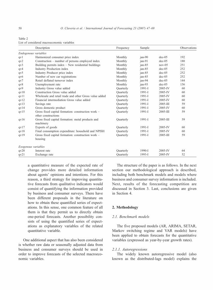
Table 2

List of considered macroeconomic variables

Description Frequency Sample Observations

Endogenous variables

qv1 Harmonized consumer price index Monthly jan-90 dec-05 192

qv2 Construction – number of persons employed index Monthly jan-91 dec-05 180

qv3 Building permits index – New residential buildings Monthly jan-85 nov-05 251

qv4 Industry Production index Monthly jan-85 dec-05 252

qv5 Industry Producer price index Monthly jan-85 dec-05 252

qv6 Number of new car registrations Monthly jan-85 dec-05 252

qv7 Retail deflated turnover index Monthly jan-94 dec-05 144

qv8 Unemployment rate Monthly jan-93 dec-05 156

qv9 Industry Gross value added Quarterly 1991-I 2005-IV 60

qv10 Construction Gross value added Quarterly 1991-I 2005-IV 60

qv11 Wholesale and retail trade and other Gross value added Quarterly 1991-I 2005-IV 60

qv12 Financial intermediation Gross value added Quarterly 1991-I 2005-IV 60

qv13 Savings rate Quarterly 1991-I 2005-III 59

qv14 Gross domestic product Quarterly 1991-I 2005-IV 60

qv15 Gross fixed capital formation: construction work –

other constructions

Quarterly 1991-I 2005-III 59

qv16 Gross fixed capital formation: metal products and

machinery

Quarterly 1991-I 2005-III 59

qv17 Exports of goods Quarterly 1991-I 2005-IV 60

qv18 Final consumption expenditure: household and NPISH Quarterly 1991-I 2005-IV 60

qv19 Gross fixed capital formation: construction work –

housing

Quarterly 1991-I 2005-III 59

Exogenous variables

qv20 Interest rate Quarterly 1990-I 2005-IV 64

qv21 Exchange rate Quarterly 1993-I 2005-IV 52

O. Claveria et al. / International Journal of Forecasting 23 (2007) 47–6950

a quantitative measure of the expected rate of

change provides more detailed information

about agents’ opinions and intentions. For this

reason, a third strategy for improving quantita-

tive forecasts from qualitative indicators would

consist of quantifying the information provided

by business and consumer surveys. There have

been different proposals in the literature on

how to obtain these quantified series of expect-

ations. In this sense, one common feature of all

them is that they permit us to directly obtain

one-period forecasts. Another possibility con-

sists of using the quantified series of expect-

ations as explanatory variables of the related

quantitative variable.

One additional aspect that has also been considered

is whether raw data or seasonally adjusted data from

business and consumer surveys should be used in

order to improve forecasts of the selected macroeco-

nomic variables.

The structure of the paper is as follows. In the next

section our methodological approach is described,

including both benchmark models and models where

business and consumer survey information is included.

Next, results of the forecasting competition are

discussed in Section 3. Last, conclusions are given

in Section 4.

2. Methodology

2.1. Benchmark models

The five proposed models (AR, ARIMA, SETAR,

Markov switching regime and VAR models) have

been applied to obtain forecasts for the quantitative

variables (expressed as year-by-year growth rates).

2.1.1. Autoregressions

The widely known autoregressive model (also

known as the distributed-lags model) explains the

Table 3

Correspondence between business and consumer surveys indicators and the selected macroeconomic variables

Description Macroeconomic variables

v1 Economic Sentiment Indicator qv13

v2 Industrial Confidence Indicator (v7+v4�v6)/3

v3 Production trend observed in recent months qv4 qv8 qv13

v4 Assessment of order-book levels qv4 qv8 qv13

v5 Assessment of export order-book levels qv4 qv8 qv13 qv16

v6 Assessment of stocks of finished products qv4 qv8 qv13

v7 Production expectations for the months ahead qv4 qv8 qv13

v8 Selling price expectations for the months ahead qv1 qv5

v9 Employment expectations for the months ahead qv4 qv8 qv13 qv19

v10 New orders in recent months qv4 qv8 qv15

v11 Export expectations for the months ahead qv4 qv8 qv13 qv16

v12 Consumer Confidence Indicator (v14+v16�v19+v23)/4 qv13 qv17

v13 Financial situation over last 12 months qv6 qv13 qv17

v14 Financial situation over next 12 months qv6 qv13 qv17

v15 General economic situation over last 12 months qv6 qv13 qv17

v16 General economic situation over next 12 months qv6 qv13 qv17

v17 Price trends over last 12 months qv1

v18 Price trends over next 12 months qv1

v19 Unemployment expectations over next 12 months qv13 qv17 qv19

v20 Major purchases at present qv13 qv17

v21 Major purchases over next 12 months qv13 qv17

v22 Savings at present qv12

v23 Savings over next 12 months qv12

v24 Statement on financial situation of household qv12

v25 Intention to buy a car within the next 2 years qv6

v26 Purchase or build a home within the next 2 years qv18

v27 Home improvements over the next 12 months qv18

v28 Construction Confidence Indicator (v30+v31)/2 qv3 qv10 qv14 qv15 qv19

v29 Trend of activity compared with preceding months qv3 qv10 qv14 qv15 qv19

v30 Assessment of order books qv3 qv10 qv14 qv15 qv19

v31 Employment expectations for the months ahead qv2 qv8

v32 Price expectations for the months ahead qv1

v33 Retail Trade Confidence Indicator (v34�v35+v37)/3 qv11 qv14

v34 Present business situation qv11 qv14

v35 Assessment of stocks qv11

v36 Orders placed with suppliers qv11

v37 Expected business situation qv11 qv14

v38 Employment qv8

v39 Services Confidence Indicator (v40+v41+v42)/3 qv11 qv12 qv14

v40 Assessment of business climate qv11 qv12 qv14

v41 Evolution of demand in recent months qv11 qv12 qv14

v42 Evolution of demand expected in the months ahead qv11 qv12 qv14

v43 Evolution of employment in recent months qv8

v44 Evolution of employment expected in the months ahead qv8

O. Claveria et al. / International Journal of Forecasting 23 (2007) 47–69 51

behaviour of the endogenous variable as a linear

combination of its own past values:

xt ¼ /1xt�1 þ /2xt�2 þ : : : þ /pxt�p þ et ð1Þ

The key question is how to determine the number

of lags that should be included in the model. For

monthly data, we have considered different models

with a minimum of 1 lag and a maximum of 24

lags (including all the intermediate lags), selecting

the model with the lowest value of the Akaike

Information Criteria (AIC). For quarterly data, we

have considered a maximum number of lags of 8.

O. Claveria et al. / International Journal of Forecasting 23 (2007) 47–6952

2.1.2. ARIMA models

Since the work by Box and Jenkins (1970),

ARIMA models have been widely used and their

forecasting performance has also been confirmed.

The general expression of an ARIMA model is the

following:

xkt ¼

Hs Lsð Þh Lð Þ

Us Lsð Þ/ Lð ÞDDs D

det ð2Þ

where

Hs Lsð Þ ¼ 1�HsL

s �H2sL2s � : : : �HQs

LQs��ð3Þ

is a seasonal moving average polynomial,

Us Lsð Þ ¼ 1� UsL

s � U2sL2s � : : : � UPs

LPs��

ð4Þ

is a seasonal autoregressive polynomial,

h Lð Þ ¼ 1� h1L1 � h2L

2 � : : : � hqLq��

ð5Þ

is a regular moving average polynomial,

/ Lð Þ ¼ 1� /1L1 � /2L

2 � : : : � /pLp��

ð6Þ

is a regular autoregressive polynomial, k is the value

of the Box and Cox (1964) transformation, DsD is the

seasonal difference operator, Dd is the regular diffe-

rence operator, S is the periodicity of the considered

time series, and et is the innovation which is assumed

to behave as a white noise.

In order to use this kind of models for forecasting

purposes it is necessary to identify the best suited

model (i.e., to give values to the order of the different

polynomials, to the difference operator, etc.). For

monthly data, we have considered models with up to

12 AR and MA terms (4 in the case of quarterly data)

selecting the model with the lowest value of the AIC.

The statistical goodness of the selected model has also

been checked.

2.1.3. TAR models

In the case of the ARIMA model the relationship

between the current value of a variable and its lags is

supposed to be linear and constant over time.

However, when looking at real data it can be seen

that expansions are more prolonged over time than

recessions (Hansen, 1997). In fact, in the behaviour of

most economic variables, there seems to be a cyclical

asymmetry that lineal models are not able to capture

(Clements & Smith, 1999).

A self-excited threshold autoregressive model

(SETAR) for the time series xt can be summarised

as follows:

B Lð Þxt þ ut if xt�kV x ð7Þ

f Lð ÞSt þ mt if xt�kN x ð8Þ

where ut and mt are white noises, B(L) and f(L) areautoregressive polynomials, the value k is called the

delay and the value x is called the threshold.

This two-regime self-exciting threshold autoregres-

sive process is estimated using monthly and quarterly

data for each indicator and the Monte Carlo procedure

is used to generate multi-step forecasts.

The selected values of the delay are those minimis-

ing the sum of squared errors among values between 1

and 12 for monthly data and 1 and 4 for quarterly data.

2.1.4. Markov switching regime models

Threshold autoregressive models are perhaps the

simplest generalization of linear autoregressions. In

fact, these models were built on developments over

traditional ARMA time series models. As an alternative

to these models, time series regime-switching models

assume that the distribution of the variable is known

conditional on a particular regime or state occurring.

When the economy changes from one regime to

another, a substantial change occurs in the series.

Hamilton (1989) presented the Markov regime-

switching model in which the unobserved regime

evolves over time as a 1st-order Markov process. The

regime completely governs the dynamic behaviour of

the series. This implies that once we condition on a

particular regime occurring, and assume a particular

parameterization of the model, we can write down the

density of the variable of interest. However, as the

regime is strictly unobservable, it is necessary to draw

statistical inferences regarding the likelihood of each

regime occurring at any point in time. So, it is

necessary to obtain the transition probabilities from

one regime to the other.

There have been three different approaches to

estimating these models (Potter, 1999). First, Hamilton

Table 4

VAR models specification

VAR model Considered quantitative variables

Total of the economy Harmonized consumer price

index

Gross domestic product

Unemployment rate

Supply Industry Gross value added

Construction Gross value added

Wholesale and retail trade and

other Gross value added

Financial intermediation Gross

value added

Industry (a) Industry Production index

Industry Producer price index

Industry (b) Industry Production index

Industry Producer price index

Gross fixed capital formation:

metal products and machinery

Building Construction – number of

persons employed index

Building permits index – New

residential buildings

Gross fixed capital formation:

construction work – other

constructions

Gross fixed capital formation:

construction work – housing

Interest rates

Exports Gross domestic product

Exports of goods

Exchange rates

Consumption Harmonized consumer price

index

Gross domestic product

Final consumption expenditure:

household and NPISH

Unemployment rate

Interest rates

Savings Harmonized consumer price

index

Savings rate

Gross domestic product

Interest rates5 The Hamilton filter is an iterative procedure which provides

estimates of the probability that a given state is prevailing at each

point in time given its previous history. These estimates are

dependent upon the parameter values given to the filter. Running

the filter through the entire sample provides a log likelihood value

for the particular set of estimates used. This filter is then repeated to

optimise the log likelihood to obtain the MLE estimates of the

parameters. With the maximum likelihood parameters, the proba-

bility of being in state 0 at each point in time is calculated and these

are the probabilities of recession and expansion.6 An alternative approach would have consisted in imposing the

values of P and k instead of estimating them. These models are

known as Markov switching autoregressive models (MS-AR) and,

in general, the values of P are 0.7 or 0.8 and the values of k, 0 or 1.

O. Claveria et al. / International Journal of Forecasting 23 (2007) 47–69 53

(1989) developed a nonlinear filter for evaluating the

likelihood function of the model and then directly

maximized the likelihood function. Second, in a later

article, Hamilton (1990) constructed an EM algorithm

that is particularly useful for the case where all the

parameters switch. Finally, Albert and Chib (1993)

developed a Bayesian approach to estimation.

In this work, we employ a Markov-switching

threshold autoregressive model (MK-TAR) where

we allow for different regime-dependent intercepts,

autoregressive parameters, and variances. The estima-

tion of the models is carried out by maximum

likelihood using the Hamilton (1989) filter5 together

with the smoothing filter of Kim (1994).

Once we have estimated the probabilities of

expansion and recession, we construct the following

model for the time series xt using the estimated

probabilities of changing regime:

B Lð Þxt þ ut if P Expansion=xt�k½ �VP ð9Þ

f Lð Þxt þ mt if P Expansion=xt�k½ �NP ð10Þ

where, as in SETAR models, ut and mt are white

noises, B(L) and f(L) are autoregressive polynomials,

the value k is known as delay and the value P is

known as threshold.6 The selected values of the delay

are those minimising the sum of squared errors among

values between 1 and 12 for monthly data and 1 and 4

for quarterly data. The values of the threshold are

given by the variation of the probability.

2.1.5. VAR models

The VAR models that have been specified try to

pick up, as far as possible, the classical Economic

Theory assumptions in order to reflect the economic

dynamics. In this sense, the VAR models that have

been estimated could be defined as btotal of the

economyQ, bsupplyQ, bindustryQ, bconstructionQ and, onthe demand side, bexportsQ, bconsumptionQ and

bsavingsQ. In particular, the considered quantitative

VAR models are shown in Table 4.

O. Claveria et al. / International Journal of Forecasting 23 (2007) 47–6954

2.2. Models where business and consumer surveys

information is incorporated

2.2.1. bAugmentedQ autoregression, Markov switching

regime and VAR models

One way to use the information of the qualita-

tive indicators to improve the forecasts of the

quantitative variables is to introduce selected

indicators as explanatory variables in autoregression

and VAR models. Recently, different works have

estimated autoregressive and VAR models for some

target variable (consumer spending, GNP), adding

current and lagged values of a consumer confidence

index to the models in order to test its significance

and consider the extent of its effects. The approach

applied in this section is quite similar. In this

context, it is worth mentioning that, as shown in

Table 2, more than one quantitative variable could

be related to the evolution of the considered

indicators. So, different possibilities have been

considered for each autoregressive model. For the

case of baugmentedQ VAR models, the strategy has

been slightly different: only selected indicators

have been included. This information is shown in

Table 5.

2.2.2. Leading indicator models

In spite of their well-known limitations pointed out

in the literature, leading indicators can also provide

reliable forecasts of the analysed quantitative varia-

bles by considering the whole set of information of

business and consumer surveys.

Table 5

Specification of baugmentedQ VAR models

Macroeconomic variables

Total qv1 qv14 qv8

Supply qv9 qv10 qv11 qv12

Industry (a) qv4 qv5

Industry (b) qv4 qv5 qv16

Building (a) qv2 qv3 qv15 qv19

Building (b) qv2 qv3 qv15 qv19

Exports qv14 qv17 qv21

Consumption

(a)

qv1 qv8 qv14 qv18

Consumption

(b)

qv1 qv8 qv14 qv18

Savings qv1 qv13 qv14 qv20

According to Clements and Hendry (1998, p. 207)

ban indicator is any variable believed to be informa-

tive about another variable of interestQ. In this context,

a leading indicator is any variable whose outcome is

known in advance of a related variable which it is

desired to forecast. Usually, there are several leading

indicators for every variable to be forecasted, and for

this reason, composite leading indicators are con-

structed. A composite leading index is a combination

(e.g. a weighted average) of this set of simple leading

indicators. Composite leading indicators are useful for

providing estimates of the current state and short-term

forecasts of the analysed economy. The main advan-

tage of composite leading indicators in relation to

other methods is that it is not necessary to obtain

forecasts for exogenous variables as their lagged

values are known in advance. Of course, leading

indicators will only provide reasonably accurate short-

term forecasts. However, we extend the analysis up to

2 years as an additional benchmark for the results

using other procedures.

The procedure for the selection of the simple

leading indicators for each endogenous variable is

based on the bilateral correlations between different

lags of each of the variables in the business and

consumer survey indicators and the endogenous

variable. The simple leading indicators have been

chosen from among those with the highest values of

the correlation coefficient. The length of the lead has

been determined by cross-correlation analysis. In this

sense, as an automatic identification procedure,

different values of the bilateral correlation coefficient

Indicators

v1

v1

v7b v8b

v2

qv20 v28

qv20 v31b v32b

v5b

qv20 v12

qv20 v14b v16v v18b v19b

v23b v24b

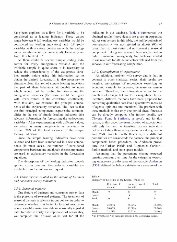
Table 6

Summary of the results of the Kruskal–Wallis test

Rejection of

the null

Non-rejection of

the null

Total

Month 9 30 39

Quarter 1 4 5

Total 10 34 44

Month 23.08% 76.92% 100.00%

Quarter 20.00% 80.00% 100.00%

Total 22.73% 77.27% 100.00%

Null hypothesis: Non-seasonal pattern in the considered series.

O. Claveria et al. / International Journal of Forecasting 23 (2007) 47–69 55

have been explored as a limit for a variable to be

considered as a leading indicator. These values

range between 0 (all explanatory variables would be

considered as leading indicators) and 0.8 (only

variables with a strong correlation with the endog-

enous variable would be considered). Eventually we

fixed this limit at 0.5.

As there could be several simple leading indi-

cators for every endogenous variable and the

available sample is quite short, it is necessary to

reduce the dimensionality of the exogenous varia-

bles matrix before using this information set to

obtain the desired forecasts. It is also necessary to

eliminate from this set of simple leading indicators

the part of their behaviour attributable to noise

which would not be useful for forecasting the

endogenous variables (the noise would be higher

with lower values of the correlation coefficient).

With this aim, we extracted the principal compo-

nents of the explanatory variables. The idea is that

the first principal components capture the common-

alities in the set of simple leading indicators (the

relevant information for forecasting the endogenous

variables). After experimenting with different values,

we retain as many components as necessary to

explain 70% of the total variance of the simple

leading indicators.

Once the simple leading indicators have been

selected and have been summarised in a few compo-

nents (in most cases, the number of considered

components between one and three), these components

are used as explanatory variables in the forecasting

equations.

The description of the leading indicator models

applied in this case and their selected variables are

available from the authors on request.

2.3. Other aspects related to the nature of business

and consumer survey indicators

2.3.1. Seasonal patterns

One feature of business and consumer survey data

is the presence of seasonal patterns. The treatment of

seasonal patterns is relevant in our context in order to

determine whether it is better to forecast macroeco-

nomic variables using raw data or seasonally adjusted

data. In order to verify the importance of seasonality,

we computed the Kruskal–Wallis test for all the

indicators in our database. Table 6 summarises the

obtained results (more details are given in Appendix

A). As can be seen in this table, the null hypothesis of

non-seasonality was not rejected in almost 80% of

cases, that is, most series did not present a seasonal

component. Taking into account these results, and in

order to maintain homogeneity, Surinach we decided

to use raw data for all the indicators obtained from the

surveys in our forecasting competition.

2.3.2. Quantification of expectations

An additional problem with survey data is that, in

contrast to other statistical series, their results are

weighted percentages of respondents expecting an

economic variable to increase, decrease or remain

constant. Therefore, the information refers to the

direction of change but not to its magnitude. In the

literature, different methods have been proposed for

converting qualitative data into a quantitative measure

of agents’ opinions and intentions. The problem with

these methods is that only one-period-ahead forecasts

can be directly computed (for further details, see

Claveria, Pons, & Surinach, in press), and for this

reason, in this paper the quantification of expectations

will only be used to transform survey indicators

before including them as regressors in autoregression

and VAR models. With this aim, six different

possibilities are considered: the balance, the principal

components based procedure, the Anderson proce-

dure, the Carlson–Parkin and Augmented Carlson–

Parkin methods and state space models.

Assuming that the percentage change expected

remains constant over time for the categories expect-

ing an increase or a decrease of the variable, Anderson

(1951) defined the balance statistic as a measure of the

O. Claveria et al. / International Journal of Forecasting 23 (2007) 47–6956

average changes expected in the variable. Ever since,

the balance statistic has been widely used as a short-

term forecast as well as for the construction of several

economic indicators.

There have been a variety of quantification methods

proposed in the literature. These methods are based on

the assumption that respondents base their answer on a

subjective probability distribution defined over future

changes in the variable and conditional on the

information available up to that moment, which has

the same form for all agents. Differences between

methods have usually been related to theoretical

considerations regarding rationality tests rather than

based on their forecasting ability.

The accuracy of the balance statistic as a means for

extracting the maximum degree of information from

survey data on the direction of change has been widely

studied since the introduction of this new source of

information in Europe by the IFO-Institut fur Wirt-

schaftsforschung at the beginning of the fifties, for

example by Anderson (1951, 1952), Theil (1952,

1955), Anderson, Bauer, and Fels (1954), De Menil

and Bhalla (1975) and Defris and Williams (1979).

This line of research has led some authors to look

for alternative procedures and statistics oriented

towards the conversion of qualitative data into

quantitative series of expectations.

While most of the emphasis was given to the

justification of the balance statistic within a theoret-

ical framework and the evaluation of its performance

as a predictor of inflation and economic activity, as

well as to the analysis of the rationality and the

formation of expectations (i.e. Papadia, 1983), some

other studies have been more empirically oriented.

The fact that business and consumer surveys seem to

be a valuable tool for anticipating economic activity

has given rise to a line of research more focused on

the construction of indexes and indicators of activity

with survey data.

In spite of the valuable information contained in

the balance statistic, our experience with this type of

data has led us to find some limitations with the

balance statistic as a forecasting measure. Some of

these shortcomings concerning the degree of re-

sponse, the relative importance of each category for

every question, etc., depend to a large extent on the

specific features of the survey under consideration.

Some other problems, such as the volatility and the

escalation of the series, are related to the nature of

the data and the direction of change.

For this reason, we have considered other possibil-

ities of bquantifyingQ the information from business and

consumer surveys. A first possibility consists of

summarising all the possible answering categories

contained in the business and consumer surveys in an

indicator that also takes account of the percentage of

bstableQ answers. This indicator can be constructed usinga principal component analysis (PCA) of all the answers

for each question, which shows the linear combination

of the three/five/six percentages that captures the

maximum variability between the successive surveys.

However, the strong correlation of the balance

statistic and the percentage changes of its corres-

ponding quantitative index of reference found by

Anderson (1952) opened the door for the quantifica-

tion of ordinal responses using more complex

methods. Theil (1952) suggested a theoretical frame-

work, later referred to as the subjective probability

approach, to convert qualitative responses about the

direction of change into quantitative expectations,

xt�1e . The basic idea behind the method is that there is

some indifference interval around zero within which

respondents report bno changeQ, whereas outside theyreport a change in the variable.

Let xt�1 be the percentage change of the variable

from period t to period t+1 and xt�1e its expectation

conditional on the respondent’s information set. Hence,

an expected increase is reported if xt�1e Nda with a

relative frequency Att+1 and an expected decrease

xt�1e Nda with a relative frequency Bt

t+1. Assuming the

standard normal distribution, one can derive:

xetþ1 ¼ ddgtþ1t ð11Þ

where gtþ1t ¼ btþ1t þ atþ1t

btþ1t � atþ1t

and

btþ1t ¼ U�1 Btþ1t

� �¼� d� xxetþ1

retþ1

atþ1t ¼ U�1 1� Atþ1t

� �¼

d� xxetþ1retþ1

:

8>>><>>>:

U�1 stands for the inverse of the cumulative standard

normal distribution. As pointed out by Zimmermann

(1999), the logistic and the scaled-t have also been used

in the literature, usually leading to very similar results.

Since the limit of the interval of indifference y is

O. Claveria et al. / International Journal of Forecasting 23 (2007) 47–69 57

unknown, Carlson and Parkin (1975) used the follow-

ing method of scaling:

dd ¼

Xnt¼1

xtþ1

Xnt¼1

gtþ1t

: ð12Þ

This method was first applied by Carlson and Parkin

(1975) and has been widely employed in the literature

ever since. Recent contributions have relaxed the

assumption of a symmetric indifference interval and

the unbiasedness condition introduced by the Carlson–

Parkin escalating procedure:

xxetþ1 ¼ ddbetþ1t þ ddaf

tþ1t ð13Þ

when etþ1t ¼ btþ1t

btþ1t � atþ1t

and f tþ1t ¼ atþ1t

btþ1t � atþ1t

:

As parameters db and da are unknown, they have

to be estimated, usually by the OLS regression

xt ¼ dbet�1t þ daf t�1t þ ut. This alternative procedure

implies that the aggregate distribution and the indif-

ference intervals are the same for both expectations

and realizations. As happened with Carlson–Parkin

method, this may cause problems when using the

derived data for testing the rationality of expectations.

Recent econometric techniques have been incor-

porated in the methodology in order to overcome

some of its shortcomings, basically the restrictive

assumptions on which it is based. As a result, new

methods have been suggested and applied with the

aim of obtaining accurate series of expectations.

Recent papers have focused on the possibility of

using state space models to estimate series of expect-

ations and to forecast reference quantitative variables.

For example, Seitz (1988) applied the time-varying

parameter model of Cooley and Prescott (1976) and

used the Kalman filter to derive a dynamic and

asymmetric indifference interval.

Our proposal consists on using a state space model

where the Kalman filter is used to estimate time

varying and asymmetric indifference intervals that can

be used to obtain series of expectations but also to

forecast reference quantitative series.

By relaxing the assumption that thresholds da,t+1

and db,t+1 are symmetric and are fixed across time, the

asymmetric Carlson–Parkin conversion equation turns

into:

xxetþ1 ¼ ddb;tþ1 þ dda;tþ1 ð14Þ

where etþ1t ¼ btþ1t

btþ1t � atþ1t

and f tþ1t ¼ atþ1t

btþ1t � atþ1t

:

Instead of using the Cooley and Prescott time-

varying parameter model and regressing the observed

percentage change of the variable on retrospective

survey responses in order to obtain estimates of xt+1e

as done by Seitz (1988), we propose a more general

state space representation for the threshold parameters

that would include Seitz’s method as a particular case:

xxt ¼ da;tett�1 � db;t f

tþ1t þ ut ð15Þ

where ut ~N(0,ru2), and

da;t ¼ ada;t�1 þ mtdb;t ¼ bdb;t�1 þ wt

�ð16Þ

where a and b are the autoregressive parameters and

vt and wt are two independent and normally distrib-

uted disturbances with mean zero and variance rv2 and

rw2 , respectively. The relationship between xt and the

response thresholds is linear and it is expressed in the

measurement equation. The unknown state is sup-

posed to vary in time according to the linear transition

equation. The Kalman filter is used in order to

estimate the variances and the autoregressive param-

eters, and derive estimates of xt+1e .

This generalization of the probability approach

introduces a more flexible representation, allowing

for asymmetric and dynamic response thresholds

generated by a first-order Markov process. Addition-

ally, estimates of xt+1e can be derived by means of

survey responses about expectations alone, without

the need for perceptions about past changes of the

variable.

We also consider a particular case of this general

model where threshold parameters follow a random

walk instead of an autoregressive process. Therefore,

O. Claveria et al. / International Journal of Forecasting 23 (2007) 47–6958

a and b are supposed to be zero and the state space

representation of the model is:

xxt ¼ da;tett�1 � db;t f

tþ1t þ ut ð17Þ

where ut ~N(0,ru2), and

da;t ¼ da;t�1 þ mtdb;t ¼ db;t�1 þ wt

�ð18Þ

When initialising the Kalman filter two options have

been considered. First, we have supposed that the

initial conditions of the filter are obtained by

regressing xt on ett+1 and f t

t+1 in the first quarter of

the sample. We have also supposed that both initial

conditions are equal to zero. As a result, we end up

with four different state space representations:

SS1: autoregressive process with initial conditions

estimated by OLS regression.

Table 7

Summary of the results from the forecasting competition

Monthly models

1 month 2 months

Non-survey AR qv1, qv3, qv5,

qv6, qv7, qv8

qv1, qv3, qv

qv7, qv8

ARIMA

TAR

MK-TAR

VAR

Survey AR qv4 qv4

MK-TAR

VAR

Leading

indicator

qv2 qv2, qv6

Quarterly models

1 quarter

Non-survey AR qv10

ARIMA

TAR

MK-TAR

VAR qv14, qv15, qv16,

qv19

Survey AR

MK-TAR qv9

Leading

indicator

qv11, qv13, qv17,

qv18, qv19

VAR qv12

SS2: random walk process with initial conditions

estimated by OLS regression.

SS3: random walk process with null initial conditions.

SS4: autoregressive process with null initial conditions.

Further details on the estimation procedure can be

found in Harvey (1982, 1987).

The output of these quantification procedures can be

considered either as one period ahead forecasts of the

quantitative variable used in the analysis or as exoge-

nous proxies (quantified indicators) introduced in AR

and VAR models to forecast quantitative variables. This

second alternative is the one considered in this paper.

3. Results of the forecasting competition

In order to evaluate the relative forecasting accuracy

of the models, all models were estimated until 2001.12

(or 2001.III or IV for quarterly indicators) for each

3 months 6 months 12 months

5, qv1, qv3, qv5,

qv6, qv7, qv8

qv1, qv6, qv7 qv1

qv4 qv4 qv7, qv8

qv4

qv2 qv2, qv3, qv5,

qv8

qv2, qv3,

qv5, qv6

2 quarters 4 quarters

qv10

qv9

qv15 qv14, qv18

qv16 qv10, qv17

qv9

qv13, qv14, qv17,

qv18, qv19

qv12, qv13

qv11, qv12 qv11, qv15, qv16

7 We are grateful to an anonymous referee for this suggestion.8 This measure has been calculated using the Stata routine of

Christopher F. Baum which is available at http://fmwww.bc.edu/

repec/bocode/d/dmariano.ado and http://fmwww.bc.edu/repec/

bocode/d/dmariano.hlp.

O. Claveria et al. / International Journal of Forecasting 23 (2007) 47–69 59

variable to be forecasted and forecasts for 1, 2, 3, 6 and

12 months (or 1, 2, 4 quarters) ahead were computed.

The specifications of the models are based on

information up to that date, and then, models are re-

estimated in each month or quarter and forecasts are

computed. Given the availability of actual values until

2005.12 or 2005.III or IV, forecast errors for each

indicator and method can be computed in a recursive

way (i.e., for the 1-month forecast horizon, 48 forecast

errors can be computed for each indicator or 16 for the

1-quarter forecast horizon). In order to summarise this

information, the root mean square error (RMSE) has

been computed. These values provide useful informa-

tion for analysing the forecast accuracy of eachmethod,

somethods can be ranked according to their values. It is

worth mentioning that we have assumed that in all

cases the information of business and consumer

surveys is known in advance, which is not a strong

assumption for shorter forecast horizons but could be

for longer ones. A possible strategy that is beyond the

scope of this paper is to apply univariate forecasting

methods to business and consumer survey indicators

(see Clar, Duque, & Moreno, in press).

The results of our forecasting competition are

shown in Tables B.1 to B.19 of Appendix B. These

tables present the values of the root mean square error

(RMSE) obtained from recursive forecasts for 1, 2, 3,

6 and 12 months during the period 2002.1–2005.12 or

for 1, 2 and 4 quarters during the period 2002.I–

2005.IV for both the benchmark models and the

models including information from surveys.

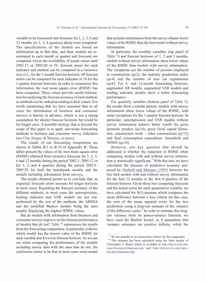
The results obtained permit us to conclude that, as

expected, forecasts errors increase for longer horizons

in most cases. Regarding the forecast accuracy of the

different methods, in most cases the autoregression,

leading indicator and VAR models are not out-

performed by the rest of the methods, the ARIMA

and the modified Markov models being the ones

usually displaying the highest RMSE values.

But do models with information from business and

consumer surveys improve on the forecast performance

of models that do not? Table 7 summarises the results

from the forecasting competition. In particular, it shows

which model has the lowest value of the RMSE for

each variable and for every forecast horizon. As we can

see when comparing the performance of the models

including survey data with the ones that do not, the

conclusion seems to be that in most cases some model

that includes information from the survey obtains lower

values of the RMSE than the best model without survey

information.

In particular, for monthly variables (top panel of

Table 7) and forecast horizons of 1, 2 and 3 months,

models without survey information show lower values

of the RMSE than models with survey information.

The exceptions are the number of persons employed

in construction (qv2), the industry production index

(qv4) and the number of new car registrations

(qv6). For 6- and 12-month forecasting horizons,

augmented AR models, augmented VAR models and

leading indicator models show a better forecasting

performance.

For quarterly variables (bottom panel of Table 7),

the results show a similar pattern: models with survey

information show lower values of the RMSE, with

some exceptions for the 1 quarter forecast horizon. In

particular, autoregression and VAR models without

survey information achieve better results for gross

domestic product (qv14), gross fixed capital forma-

tion: construction work – other constructions (qv15)

and final consumption expenditure: household and

NPISH (qv18).

However, one key question that should be

addressed is whether the reduction in RMSE when

comparing models with and without survey informa-

tion is statistically significant.7 With this aim, we have

calculated the measure of predictive accuracy pro-

posed by Diebold and Mariano (1995) between the

two best models with and without survey information

for the first 12 months or the first 4 quarters of the

forecast horizon. Given these two competing forecasts

and the actual series for each quantitative variable, we

have calculated the S(1) measure which compares the

mean difference between a loss criteria (in this case,

the root of the mean squared error) for the two

predictions using a long-run estimate of the variance

of the difference series.8 In order to estimate this long-

run variance from its autocovariance function, we

have used the Bartlett kernel, as it guarantees that

variance estimates are positive definite, while the

Table 8

Results of the Diebold–Mariano test

Monthly data: 2002m1–2002m12 Quarterly data: 2002q1–2002q4

qv1 �1.26 qv9 �0.12qv2 �2.24* qv10 �1.92qv3 0.29 qv11 �0.01qv4 �1.72 qv12 1.02

qv5 �3.81* qv13 3.84*

qv6 3.81* qv14 �2.18*qv7 2.97* qv15 3.14*

qv8 2.64* qv16 �2.45*qv17 �1.49qv18 �1.67qv19 �10.88*

Null hypothesis: The difference between the two competing series is

non-significant.

A positive sign of the statistic implies that the RMSE associated to

the forecast from the model with survey information is lower while

a negative sign implies the opposite.

* Significant at the 5% level. Bold indicates positive and

significant results.

O. Claveria et al. / International Journal of Forecasting 23 (2007) 47–6960

maximum lag order has been calculated using the

Schwert criterion as a function of the sample size.

These results are shown in Table 8.

If we look at the results from Table 8, we can see

that in 9 out of 19 cases there is no significant

difference between the forecasts. However, in ten

cases, the difference is significant and in five of them,

this difference is in favour of the model with survey

information.9 The actual values and the two compet-

ing forecasts for these ten series where the difference

is significant are shown in Fig. 1.

As we can see from Table 8 and Fig. 1, the

consideration of information from business and

consumer surveys significantly improves the forecast-

ing performance of the considered models, but in a

similar number of cases than models without survey

information. These results are in line with the ones

shown in Table 7 and Appendix B.

However, looking at Fig. 1, it can also be observed

that information from business and consumer surveys

is particularly helpful in the presence of turning points

9 We have carried out a similar analysis for different periods and

results have been similar. For example, using information up to

2000.12 or 2000.IV for estimating the model and forecasts until

2001.12 or 2001.IV, in 12 out of 19 cases there is no significant

difference between forecasts including survey information or not.

However, in seven cases the difference is significant, and in five of

them this difference is in favour of themodelwith survey information.

in the forecasting horizon. For example, in the case of

the savings rate (qv13), the leading indicator model

with survey information is able to capture the

downward trend in its evolution more quickly. A

similar result is obtained for the gross fixed capital

formation (qv15) when the construction confidence

indicator (v28) is included as an exogenous variable

in a VAR model.

Summarising, the comparison of the forecasting

performance of the two sets of models permits us to

conclude that in most cases, models that include

information from the surveys obtain lower values of

the RMSE than the best model without survey

information, particularly at longer forecasting hori-

zons. However, this reduction is only significant in a

limited number of cases. In this sense, the results

obtained extend the results of previous research that

have considered information from business and

consumer surveys to explain the behaviour of

macroeconomic variables, but are not conclusive

about its role.

4. Conclusions

The objective of this paper was to analyse the

possibility of improving the forecasts for some selected

macroeconomic variables for the euro area using the

information provided by business and consumer

surveys. With this aim, we have carried out a fore-

casting competition between models with and without

survey information, considering the presence or

absence of seasonal patterns in the data and the need

of quantifying the information from surveys.

The results obtained allow us to conclude that the

consideration of information from business and

consumer surveys has only improved in a limited

number of cases the forecasting performance of the

different models for the considered macroeconomic

variables significantly.

Last, it is important to highlight that we have

extended in a more systematic way10 the results of

10 To our knowledge, no other study covers such a large number

of macroeconomic variables and indicators (attention has been

usually paid to industrial production, inflation and GDP). The

number of econometric methods and models applied is also

considerably higher than in previous research.

Fig. 1. Comparison of actual values and significantly different competing forecasts according to the Diebold–Mariano test.

O.Claveria

etal./Intern

atio

nalJournalofForeca

sting23(2007)47–69

61

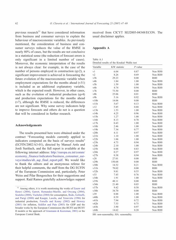
Detailed results of the Kruskal–Wallis test

Variable KW statistic P-value

v1 6.04 0.87 Non RH0

v2 8.26 0.69 Non RH0

v3b 29.23 0.00 RH0

v4b 1.84 1.00 Non RH0

v5b 1.59 1.00 Non RH0

v6b 4.74 0.94 Non RH0

v7b 73.50 0.00 RH0

v8b 25.06 0.01 RH0

v9b 5.16 0.92 Non RH0

v10b 14.06 0.00 RH0

v11b 5.67 0.13 Non RH0

v12 5.85 0.88 Non RH0

v13b 1.53 1.00 Non RH0

v14b 4.25 0.96 Non RH0

O. Claveria et al. / International Journal of Forecasting 23 (2007) 47–6962

previous research11 that have considered information

from business and consumer surveys to explain the

behaviour of macroeconomic variables. As previously

mentioned, the consideration of business and con-

sumer surveys reduces the value of the RMSE in

nearly 80% of cases, but the results are not conclusive

in a statistical sense (the reduction of forecast errors is

only significant in a limited number of cases).

Moreover, the economic interpretation of the results

is not always clear: for example, in the case of the

number of persons employed in construction (qv2), a

significant improvement is achieved in forecasting the

future evolution of the macroeconomic variable when

employment expectations for the months ahead (v31)

is included as an additional explanatory variable,

which is the expected result. However, in other cases,

such as the evolution of industrial production (qv4)

and production expectations for the months ahead

(v7), although the RMSE is reduced, the differences

are not significant. Why some survey indicators help

to improve forecasts and others do not is a question

that will be considered in further research.

v15b 1.27 1.00 Non RH0

v16b 8.13 0.70 Non RH0

v17b 0.43 1.00 Non RH0

v18b 2.46 1.00 Non RH0

v19b 7.34 0.77 Non RH0

v20b 4.11 0.97 Non RH0

v21b 1.10 1.00 Non RH0

v22b 1.06 1.00 Non RH0

v23b 4.73 0.94 Non RH0

v24b 2.10 1.00 Non RH0

v25b 0.88 0.83 Non RH0

v26b 0.27 0.97 Non RH0

v27b 0.38 0.94 Non RH0

v28 27.01 0.00 RH0

v29b 150.68 0.00 RH0

v30b 14.52 0.21 Non RH0

v31b 70.02 0.00 RH0

v32b 9.81 0.55 Non RH0

v33 7.45 0.76 Non RH0

v34b 1.91 1.00 Non RH0

v35b 48.11 0.00 RH0

Acknowledgements

The results presented here were obtained under the

contract bForecasting models currently applied to

indicators computed on the basis of surveys resultsQ(ECFIN/2002/A3-01), directed by Manuel Artıs and

Jordi Surinach, and the full report is available at the

following internet address: http://europa.eu.int/comm/

economy_finance/indicators/business_consumer_sur-

veys/studies/ub_aqr_final_report.pdf. We would like

to thank the editors and an anonymous referee for

their helpful comments, the staff from the DG ECFIN

of the European Commission and, particularly, Peter

Weiss and Pilar Bengoechea for their suggestions and

support. Raul Ramos gratefully acknowledges support

11 Among others, it is worth mentioning the works of Easaw and

Heravi (2004), Garrett, Hernandez-Murillo, and Owyang (2004),

Souleles (2004), Vuchelen (2004) for consumption, Bodo, Golinelli,

and Parigi (2000) and Kauppi, Lassila, and Terasvirta (1996) for

industrial production, Forsells and Kenny (2002) and Howrey

(2001) for inflation, Sedillot and Pain (2003) for GDP and the

broader works by the European Commission (the BUSY and BUSY

II models or the approach of Grasmann & Keereman, 2001) or the

European Central Bank.

received from CICYT SEJ2005-04348/ECON. The

usual disclaimer applies.

Appendix A

Table A.1

v36b 21.40 0.03 RH0

v37b 9.42 0.58 Non RH0

v38b 34.70 0.00 RH0

v39 0.88 1.00 Non RH0

v40b 0.39 1.00 Non RH0

v41b 7.94 0.72 Non RH0

v42b 7.53 0.75 Non RH0

v43b 3.90 0.97 Non RH0

v44b 14.62 0.20 Non RH0

H0: non-seasonality; HA: seasonality.

Table B.3

qv3: Building permits index: year-by-year growth rates of raw data

Average RMSE – recursive forecasts from December 2001 to

November 2005

1

month

2

months

3

months

6

months

12

months

O. Claveria et al. / International Journal of Forecasting 23 (2007) 47–69 63

Appendix B

Italics: best model without survey information.

Bold: better forecast performance than best model

without survey information.aBest model.

Table B.1

qv1: HCPI: year-by-year growth rates of raw data

Average RMSE – recursive forecasts from January 2002 to

December 2005

1

month

2

months

3

months

6

months

12

months

Models without survey information

AR 0.20a 0.26a 0.30a 0.30a 0.28a

ARIMA 1.55 1.85 2.18 2.32 2.53

TAR 2.04 3.12 3.91 6.03 13.13

Models with survey information

AR (+v18b) 0.20 0.26 0.33 0.41 0.58

AR

(+v18 quantified)

0.20 0.27 0.34 0.41 0.57

Leading

indicators

model 1

0.56 0.55 0.66 0.43 0.52

Leading

indicators

model 2

0.42 0.37 0.43 0.53 0.82

v18: price trends over next 12 months; b: balance.

Table B.2

qv2: Construction – number of persons employed index: year-by-

year growth rates of raw data

Average RMSE – recursive forecasts from January 2002 to

December 2005

1

month

2

months

3

months

6

months

12

months

Models without survey information

AR 0.78 0.95 1.10 1.32 1.38

ARIMA 6.19 7.93 8.75 10.14 10.66

TAR 25.89 26.49 52.13 230.52 1102.48

MK-TAR 0.99 1.35 9.25 52.58 10.76

Models with survey information

AR (+v31b) 0.77 0.93 1.05 1.24 1.15

AR

(+v31b

quantified)

0.77 0.93 1.06 1.27 1.22

Leading indicators

model 1

0.42a 0.37a 0.43a 0.53a 0.82a

Leading indicators

model 2

1.55 2.01 1.04 2.39 3.82

v31: employment expectations for the months ahead; b: balance.

Models without survey information

AR 5.55a 5.92a 6.19a 7.04 6.48

ARIMA 39.87 43.83 47.42 53.18 56.89

TAR 68.87 97.78 125.16 172.36 261.11

MK-TAR 6.47 7.98 8.98 10.20 7.83

Models with survey information

AR (+v29b) 6.47 6.93 6.96 7.71 7.07

AR (+v30b) 6.14 6.39 6.49 7.23 6.96

AR (+v29b+v30b) 5.87 6.57 6.61 7.38 6.46

AR (+v29b quantified) 6.24 6.49 6.64 7.44 7.13

AR (+v30b quantified) 5.87 6.57 6.59 7.34 6.40

Leading indicators

model 1

6.46 6.19 6.38 6.37 5.85a

Leading indicators

model 2

6.83 7.00 8.35 6.08a 7.65

v29: trend of activity compared with preceding months; v30:

assessment of order books; b: balance.

Table B.4

qv4: Industry production index: year-by-year growth rates of raw

data

Average RMSE – recursive forecasts from January 2002 to

December 2005

1

month

2

months

3

months

6

months

12

months

Models without survey information

AR 1.47 1.57 1.69 2.35 3.06

ARIMA 10.06 10.64 10.86 14.36 15.71

TAR 14.86 16.29 22.51 33.58 52.52

VAR industry (a) 1.53 1.53 1.40 1.64 1.57

Models with survey information

AR (+v7b) 1.37a 1.39a 1.39a 1.55a 1.66

AR (+v7b quantified) 1.48 1.49 1.46 1.59 1.60

Leading indicators model 1 1.45 1.53 1.44 1.96 1.38

Leading indicators model 2 1.49 1.33 1.73 1.95 2.80

VAR-industry (a)

(+v7b quantified

+v8b quantified)

1.48 1.58 1.54 1.61 1.56a

v7: production expectations for the months ahead; v8: selling price

expectations for the months ahead; b: balance.

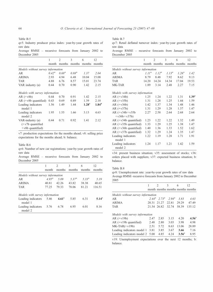
Table B.5

qv5: Industry producer price index: year-by-year growth rates of

raw data

Average RMSE – recursive forecasts from January 2002 to

December 2005

1

month

2

months

3

months

6

months

12

months

Models without survey information

AR 0.42a 0.68a 0.88a 1.37 2.04

ARIMA 2.93 4.94 6.48 10.04 15.08

TAR 4.88 6.76 8.57 15.01 23.74

VAR industry (a) 0.44 0.70 0.90 1.42 2.15

Models with survey information

AR (+v8b) 0.44 0.70 0.91 1.42 2.15

AR (+v8b quantified) 0.43 0.69 0.89 1.39 2.10

Leading indicators

model 1

1.56 1.49 1.44 1.28a 1.84a

Leading indicators

model 2

1.95 1.55 1.66 3.13 4.63

VAR-industry (a)

(+v7b quantified

+v8b quantified)

0.44 0.71 0.92 1.41 2.12

v7: production expectations for the months ahead; v8: selling price

expectations for the months ahead; b: balance.

Table B.6

qv6: Number of new car registrations: year-by-year growth rates of

raw data

Average RMSE – recursive forecasts from January 2002 to

December 2005

1

month

2

months

3

months

6

months

12

months

Models without survey information

AR 4.95a 5.09 5.37a 5.33a 5.19

ARIMA 40.81 42.26 43.82 38.38 40.65

TAR 77.25 79.33 78.06 81.21 116.51

Models with survey information

Leading indicators

model 1

5.46 4.61a 5.85 6.31 5.14a

Leading indicators

model 2

5.76 6.78 6.95 6.01 8.16

Table B.7

qv7: Retail deflated turnover index: year-by-year growth rates of

raw data

Average RMSE – recursive forecasts from January 2002 to

December 2005

1

month

2

months

3

months

6

months

12

months

Models without survey information

AR 1.11a 1.12a 1.13a 1.26a 1.42

ARIMA 8.79 8.48 7.92 8.62 9.13

TAR 14.20 14.24 14.34 17.04 19.53

MK-TAR 1.89 3.14 2.48 2.27 7.15

Models with survey information

AR (+v34b) 1.25 1.24 1.22 1.31 1.39a

AR (+v35b) 1.31 1.28 1.25 1.44 1.59

AR (+v36b) 1.42 1.37 1.34 1.48 1.46

AR (+v37b) 1.31 1.29 1.28 1.37 1.47

AR (+v34b+v35b

+v36b+v37b)

2.27 2.58 2.64 2.68 2.64

AR (+v34b quantified) 1.23 1.22 1.22 1.32 1.49

AR (+v35b quantified) 1.33 1.29 1.25 1.38 1.47

AR (+v36b quantified) 1.40 1.36 1.33 1.52 1.62

AR (+v37b quantified) 1.32 1.29 1.24 1.35 1.47

Leading indicators

model 1

1.22 1.19 1.28 1.71 1.91

Leading indicators

model 2

1.24 1.17 1.21 1.42 1.59

v34: present business situation; v35: assessment of stocks; v36:

orders placed with suppliers; v37: expected business situation; b:

balance.

Table B.8

qv8: Unemployment rate: year-by-year growth rates of raw data

Average RMSE–recursive forecasts from January 2002 to December

2005

1

month

2

months

3

months

6

months

12

months

Models without survey information

AR 2.44a 2.73a 2.94a 3.83 4.63

ARIMA 20.31 21.27 22.81 29.29 47.49

TAR 21.54 26.82 32.74 58.39 135.12

Models with survey information

AR (+v19b) 2.47 2.85 3.15 4.20 4.56a

AR (+v19b quantified) 2.48 2.80 3.03 3.98 4.98

MK-TAR(+v19b) 2.51 5.72 8.63 13.06 28.89

Leading indicators model 1 3.81 3.85 3.67 3.66 7.16

Leading indicators model 2 5.00 4.85 4.24 3.56a 8.95

v19: Unemployment expectations over the next 12 months; b:

balance.

O. Claveria et al. / International Journal of Forecasting 23 (2007) 47–6964

Table B.9

qv9: Industry Gross value added: year-by-year growth rates of raw

data

Average RMSE – recursive forecasts from 1st quarter 2002 to 4th

quarter 2005

1 quarter 2 quarters 4 quarters

Models without survey information

AR 1.79 1.98 2.11

ARIMA 8.00 9.95 10.34

TAR 16.97 16.46 15.54

MK-TAR 2.61 3.27 2.09a

VAR-supply 2.27 2.96 2.94

Models with survey information

AR (+ICI) 2.61 3.06 3.39

MK-TAR(+ICI) 2.34 2.57 2.25

Leading indicators model 1 1.57a 1.95a 3.44

Leading indicators model 2 1.69 2.55 3.16

VAR-supply (+ESI) 1.95 2.15 2.15

VAR�supply: Industry gross value addedþ Construction

þWholesale and retail tradeþ Financial intermediation

Table B.10

qv10: Construction Gross value added: year-by-year growth rates of

raw data

Average RMSE–recursive forecasts from 1st quarter 2002 to 4th

quarter 2005

1

quarter

2

quarters

4

quarters

Models without survey information

AR 1.58a 1.74a 1.99

ARIMA 8.03 9.08 11.12

TAR 12.14 15.24 19.55

MK-TAR 1.81 3.11 4.13

VAR-supply 2.28 2.96 2.94

Models with survey information

AR (+CCI) 2.24 2.29 1.55a

Leading indicators model 1 1.72 1.79 3.29

Leading indicators model 2 2.48 2.67 3.65

VAR-supply (+ESI) 1.99 1.96 1.73

VAR�supply: Industry gross value addedþ Construction

þWholesale and retail tradeþ Financial intermediation

Table B.11

qv11: Wholesale and retail trade and other gross value added: year-

by-year growth rates of raw data

Average RMSE – recursive forecasts from 1st quarter 2002 to 4th

quarter 2005

1

quarter

2

quarters

4

quarters

Models without survey information

AR 1.20 1.22 1.19

ARIMA 5.41 5.57 5.22

TAR 8.37 7.93 9.70

VAR-supply 1.24 1.16 1.42

Models with survey information

AR (+v34b) 1.17 0.99 1.08

AR (+v34b quantified) 1.16 1.00 0.99

Leading indicators model 1 0.91a 1.08 1.64

Leading indicators model 2 1.04 1.03 1.51

VAR-supply (+ESI) 1.14 0.94a 0.82a

VAR�supply: Industry gross value addedþ Construction

þWholesale and retail tradeþ Financial intermediation

v34: present business situation; b: balance.

Table B.12

qv12: Financial intermediation gross value added: year-by-year

growth rates of raw data

Average RMSE – recursive forecasts from 1st quarter 2002 to 4th

quarter 2005

1

quarter

2

quarters

4

quarters

Models without survey information

AR 1.05 1.49 1.87

ARIMA 4.28 5.99 7.73

TAR 8.25 9.69 13.36

VAR-supply 1.07 1.57 2.04

Models with survey information

AR (+v13b) 11.64 13.76 22.66

AR (+v14b) 13.62 15.47 19.29

AR (+v13b+v14b) 1.05 1.58 2.23

AR (+v13b quantified) 11.65 13.77 22.67

AR (+v14b quantified) 13.62 15.47 19.29

Leading indicators model 1 1.45 1.69 1.71a

Leading indicators model 2 1.10 1.64 1.78

VAR-supply (+ESI) 1.00a 1.42a 1.86

VAR�supply: Industry gross value addedþ Construction

þ Wholesale and retail tradeþ Financial intermediation

v13: financial situation over the last 12 months; v14: financial

situation over the next 12 months; b: balance.

O. Claveria et al. / International Journal of Forecasting 23 (2007) 47–69 65

Table B.13

qv13: Savings rate: year-by-year growth rates of raw data

Average RMSE – recursive forecasts from 4th quarter 2001 to 3rd

quarter 2005

1

quarter

2

quarters

4

quarters

Models without survey information

AR 7.94 9.70 8.27

ARIMA 32.27 42.92 50.93

TAR 53.88 58.98 62.78

VAR-savings 9.27 9.14 12.45

Models with survey information

AR (+v22b) 11.65 13.77 22.67

AR (+v23b) 13.62 15.47 19.29

AR (+v22+v23b) 17.45 17.99 22.62

AR (+v22b quantified) 11.64 13.76 22.66

AR (+v23b quantified) 13.62 14.47 19.30

Leading indicators model 1 6.73a 7.24a 7.72a

Leading indicators model 2 8.86 8.55 9.55

VAR-savings (+v23b+v24b) 8.72 9.24 10.14

VAR�savings: HCPIþ Savings rateþ GDPþ Interest rates

v22: savings at present; v23: savings over the next 12 months; v24:

statement on financial situation of household; b: balance.

Table B.14

qv14: Gross domestic product: year-by-year growth rates of raw

data

Average RMSE – recursive forecasts from 1st quarter 2002 to 4th

quarter 2005

1

quarter

2

quarters

4

quarters

Models without survey information

AR 0.94 1.02 1.11

ARIMA 4.15 4.80 4.69

TAR 7.93 10.49 14.16

MK-TAR 1.10 1.86 2.29

VAR-total 0.70a 0.67 0.76a

VAR-consumption 0.89 1.10 1.57

VAR-savings 1.28 1.67 1.88

VAR-exports 0.94 1.24 2.53

Models with survey information

AR (+ESI) 0.87 0.89 0.91

AR (+v15b) 0.90 0.90 0.94

AR (+v16b) 0.80 0.85 0.86

AR (+ESI+v15b+v16b) 1.11 1.41 1.39

AR (+v15 quantified) 0.94 1.00 1.09

AR (+v16 quantified) 0.94 1.00 1.11

MK-TAR (+v1) 1.19 1.17 1.59

Leading indicators model 1 0.96 0.64a 2.14

Leading indicators model 2 1.04 1.66 1.89

VAR-total (+ESI) 0.99 0.93 0.88

VAR-exports (+v5b) 1.01 1.13 1.82

VAR-consumption (+CCI) 0.98 1.07 0.97

VAR-consumption

(+v14b+v16b+v18b+v19b)

1.18 1.09 0.85

VAR-savings (+v23b+v24b) 1.68 1.66 1.44

VAR�total: HCPIþ GDPþ Unemployment

VAR�consumption: Consumptionþ HCPIþ GDP

þ Unemploymentþ Interest rates

VAR�savings: Savings rateþ GDPþ HCPIþ Interest rates

VAR�exports: GDPþ Exports of goodsþ Exchange rate

v14: financial situation over the next 12 months; v15: general

economic situation over the last 12 months; v16: general economic

situation over the next 12 months; v18: price trends over the next 12

months; v19: unemployment expectations over the next 12 months;

v23: savings over the next 12 months; v24: statement on financial

situation of household; b: balance.

O. Claveria et al. / International Journal of Forecasting 23 (2007) 47–6966

Table B.15

qv15: Gross fixed capital formation: construction work – other

constructions. Year-by-year growth rates of raw data

Average RMSE – recursive forecasts from 4th quarter 2001 to 3rd

quarter 2005

1

quarter

2

quarters

4

quarters

Models without survey information

AR 2.55 2.93 2.69

ARIMA 11.96 12.82 13.49

TAR 21.37 21.41 21.61

MK-TAR 2.75 3.55 3.73

VAR-building 2.06a 1.43a 3.22

Models with survey information

AR (+v29b) 2.81 2.82 3.32

AR (+v30b) 2.56 2.44 2.55

AR (+v29b+v30b) 4.80 4.93 7.00

AR (+v29b quantified) 2.76 3.33 3.29

AR (+v30b quantified) 2.57 2.66 2.74

Leading indicators model 1 2.74 2.71 2.90

Leading indicators model 2 2.88 2.88 3.84

VAR-building (a) (+CCI) 5.17 3.74 2.45a

VAR-building (b)

(+v31b+v32b)

4.76 3.05 3.85

VAR�building: Constructionþ Building permits index

þ Construction work other constructionsð Þ

þ Construction work housingð Þ

v29: trend of activity compared with preceding months; v30:

assessment of order books; v31: employment expectations for the

months ahead; v32: price expectations for the months ahead; b:

balance.

Table B.16

qv16: Gross fixed capital formation: metal products and machinery.

Year-by-year growth rates of raw data

Average RMSE – recursive forecasts from 4th quarter 2001 to 3rd

quarter 2005

1 quarter 2 quarters 4 quarters

Models without survey information

AR 2.15 3.44 4.81

ARIMA 8.41 14.31 17.32

TAR 21.73 34.09 57.61

VAR-industry (b) 1.67a 2.91 3.94

Models with survey information

AR (+v3b) 1.90 2.76a 4.21

AR (+v7b) 2.89 3.77 6.63

AR (+v3b+v7b) 5.59 9.03 37.16

AR (+v3b quantified) 1.94 2.78 4.18

AR (+v7b quantified) 3.23 3.98 5.04

MK-TAR(+v7b) 2.89 5.37 6.75

Leading indicators model 1 1.72 3.23 4.01

Leading indicators model 2 2.44 4.56 7.95

VAR-industry (b) (+ICI) 2.26 3.15 2.34a

VAR�industry ðbÞ : Industry production index

þ Industry producer price index

þ Metal products and machinery

v3: production trend observed in recent months; v7: production

expectations for the months ahead; b: balance.

Table B.17

qv17: Exports of goods: year-by-year growth rates of raw data

Average RMSE – recursive forecasts from 1st quarter 2002 to 4th

quarter 2005

1

quarter

2

quarters

4

quarters

Models without survey information

AR 3.38 5.22 6.12

ARIMA 5.62 5.68 6.61

TAR 22.23 30.80 44.41

VAR-exports 3.39 5.76 9.80

Models with survey information

AR (+11b) 4.63 6.02 5.13

AR (+v5b) 4.15 5.75 4.39a

AR (+v11b+v5b) 4.62 6.73 7.77

AR (+v11b quantified) 4.39 7.25 8.74

AR (+v5b quantified) 3.86 6.71 8.83

MK-TAR(+v11b) 3.01 5.65 6.92

Leading indicators model 1 2.98 1.90a 6.42

Leading indicators model 2 2.39a 2.68 6.58

VAR-exports (+v5b) 3.54 4.47 4.41

VAR�exports: GDPþ Exports of goodsþ Exchange rate

v5: assessment of export order-book levels; v11: export expect-

ations for the months ahead; b: balance.

O. Claveria et al. / International Journal of Forecasting 23 (2007) 47–69 67

Table B.18

qv18: Consumption: year-by-year growth rates of raw data

Average RMSE – recursive forecasts from 1st quarter 2002 to 4th

quarter 2005

1

quarter

2

quarters

4

quarters

Models without survey information

AR 1.16 1.03 0.87

ARIMA 5.62 5.67 6.60

TAR 7.65 7.15 6.42

MK-TAR 1.31 1.41 7.52

VAR-consumption 1.27 1.19 0.80a

Models with survey information

AR (+v20b) 1.14 1.01 0.92

AR (+v20b quantified) 1.19 1.06 0.86

Leading indicators model 1 1.04a 0.95a 0.84

Leading indicators model 2 1.11 1.38 1.89

VAR-consumption (a) (+CCI) 1.33 1.29 0.83

VAR-consumption (b)

(+v14b+v16b+v18b+v19b)

1.43 1.18 0.99

VAR�building: Constructionþ Building permits index

þ Construction work other constructionsð Þþ Construction work housingð Þ

v14: financial situation over next 12 months; v16: general economic

situation over next 12 months; v18: price trends over next 12

months; v19: unemployment expectations over next 12 months;

v20: major purchases at present; b: balance.

Table B.19

qv19: Gross fixed capital formation: construction work – housing.

Year-by-year growth rates of raw data

Average RMSE – recursive forecasts from 4th quarter 2001 to 3rd

quarter 2005

1

quarter

2

quarters

4

quarters

Models without survey information

AR 2.86 3.31 3.14

ARIMA 13.31 14.72 19.81

TAR 16.98 18.92 21.21

VAR building 2.78a 3.27 2.51

Models with survey information

AR (+v26b) 4.85 5.29 5.70

AR (+v26b quantified) 4.61 4.42 4.92

Leading indicators model 1 2.85 2.69a 2.45a

Leading indicators model 2 3.64 4.86 5.78

VAR building (a) (+CCI) 5.09 3.91 3.57

VAR building (b) (+v31b+v32b) 4.71 4.07 5.22

VAR�building: Constructionþ Building permits indexþ Construction work other constructionsð Þþ Construction work housingð Þ

v26: purchase or build a home within the next 2 years; v31:

employment expectations for the months ahead; v32: price expect-

ations for the months ahead; b: balance.

O. Claveria et al. / International Journal of Forecasting 23 (2007) 47–6968

References

Albert, J., & Chib, S. (1993). Bayesian inference via Gibbs

sampling of autoregressive time series subject to Markov mean

and variance shifts. Journal of Business and Economic

Statistics, 11, 1–15.

Anderson, O. (1951). Konjunkturtest und Statistik. Allgemeines

Statistical Archives, 35, 209–220.

Anderson, O. (1952). The business test of the IFO–Institute for

economic research, Munich, and its theoretical model. Revue de

l’Institut International de Statistique, 20, 1–17.

Anderson, O., Bauer, R. K., & Fels, E. (1954). On the accuracy of

short-term entrepreneurial expectations. Paper presented at the

Montreal Meeting of the American Statistical Association.

Bodo, G., Golinelli, R., & Parigi, G. (2000). Forecasting industrial

production in the Euro area. Empirical Economics, 25, 541–561.

Box, G., & Cox, D. (1964). An analysis of transformation. Journal

of the Royal Statistical Society, Series B, 211–264.

Box, G. E. P., & Jenkins, G. M. (1970). Time series analysis:

Forecasting and control. San Francisco7 Holden-Day.

Carlson, J. A., & Parkin, M. (1975). Inflation expectations.

Economica, 42, 123–138.

Clar, M., Duque, J. C., & Moreno, R. (in press). Forecasting

business and consumer surveys indicators. A time series models

competition. Applied Economics.

Claveria, O., Pons, E., & Surinach, J., (in press). Quantification

of expectations. Are they useful for forecasting inflation?

Economic Issues.

Clements, M., & Hendry, D. (1998). Forecasting economic time

series. Cambridge7 Cambridge University Press.

Clements, M., & Smith, J. (1999). A Monte Carlo study of the

forecasting performance of empirical SETAR models. Journal

of Applied Econometrics, 14, 123–141.

Cooley, T. F., & Prescott, E. C. (1976). Estimation in the

presence of stochastic parameter variation. Econometrica, 44,

167–184.

De Menil, G., & Bhalla, S. (1975). Direct measurement of popular

price expectations. American Economic Review, 65, 169–180.

Defris, L. V., & Williams, R. A. (1979). Quantitative versus

qualitative measures of price expectations. Economics Letters, 2,

169–173.

Diebold, F. X., & Mariano, R. (1995). Comparing predictive

accuracy. Journal of Business and Economic Statistics, 13,

253–263.

Easaw, J. Z., & Heravi, S. M. (2004). Evaluating consumer

sentiments as predictors of UK household consumption behav-

ior: Are they accurate and useful? International Journal of

Forecasting, 20, 671–681.

Forsells, M., & Kenny, G. (2002). The rationality of consumer’s

inflation expectations: Survey-based evidence for the euro area.

ECB Working Paper, 163.

Garrett, T. A., Hernandez-Murillo, R., &Owyang,M. T. (2004). Does

consumer sentiment predict regional consumption? Review–

Federal Reserve Bank of St. Louis, 87, 123–135.

Grasmann, P., & Keereman, F. (2001). An indicator-based short-

term forecast for quarterly GDP in the euro area. Economic

Paper, 154.

O. Claveria et al. / International Journal of Forecasting 23 (2007) 47–69 69

Hamilton, J. (1989). A new approach to the economic analysis of

nonstationary time series and the business cycle. Econometrica,

57, 357–384.

Hamilton, J. (1990). Analysis of time series subject to changes in

regime. Journal of Econometrics, 45, 39–70.

Hansen, B. (1997). Inference in threshold models. Unpublished

manuscript.

Harvey, A. (1982). The Kalman filter and its applications in

econometrics and time series analysis. Methods of Operational

Research, 44, 3–18.

Harvey, A. (1987). Applications of the Kalman filter in economet-

rics. In T. Bewley (Ed.), Advances in econometrics: Fifth World

Congress, Econometric Society Monograph, vol. 13.

Cambridge7 Cambridge University Press.

Howrey, E. P. (2001). The predictive power of the index of

consumer sentiment. Brookings Papers on Economic Activity, 1,

205–207.

Kauppi, E., Lassila, J., & Terasvirta, T. (1996). Short-term

forecasting of industrial production with business survey data:

Experience from Finland’s great depression 1990–1993. Inter-

national Journal of Forecasting, 12, 373–381.

Kim, C. J. (1994). Dynamic linear models with Markov-Switching.

Journal of Econometrics, 60, 1–22.

Papadia, F. (1983). Inflationary expectations in the European

economic communities countries. Empirical Economics, 8,

187–202.

Pesaran, M. H. (1987). The limits to rational expectations. Oxford7

Basil Blackwell.

Potter, S. (1999). Nonlinear time series modelling: An introduction.

Federal Reserve Bank of New York, Mimeo.

Sedillot, F., & Pain, N. (2003). Indicators models of real GDP

growth in selected OECD countries. ECO Working Paper, 364.

Seitz, H. (1988). The estimation of inflation forecasts from business

survey data. Applied Economics, 20, 427–438.

Souleles, N. S. (2004). Expectations, heterogeneous forecast errors,

and consumption: Micro evidence from the Michigan consumer

sentiment surveys. Journal of Money, Credit, and Banking, 36,

39–72.

Theil, H. (1952). On the time shape of economic microvariables and

the Munich business test. Revue de l’Institut International de

Statistique, 20, 105–120.

Theil, H. (1955). Recent experiences with the Munich business test:

An expository article. Econometrica, 23, 184–192.

Vuchelen, J. (2004). Consumer sentiment and macroeconomic

forecasts. Journal of Economic Psychology, 25, 493–506.

Zimmermann, K. F. (1999). Analysis of business surveys. In M. H.

Pesaran, & P. Schmidt (Eds.), Handbook of applied economet-

rics, volume II: Macroeconomics. Oxford7 Blackwell Publishers.

Oscar Claveria. Research fellow at the Grup d’Analisi Quantitativa

Regional and assistant professor in the Department of Econometrics

at the University of Barcelona. His teaching areas are mainly in

Statistics and Econometrics. His research interests are focused on

forecasting quantitative and qualitative variables, econometrics and

time series methods and conjuncture analysis. He has collaborated

in different research projects related to the quantification of

expectations and has published part of his research in Cuadernos

Aragoneses de Economıa and Economic Issues.

Ernest Pons. Research fellow at the Grup d’Analisi Quantitativa

Regional and assistant professor in the Department of Econometrics

at the University of Barcelona. His teaching areas are mainly in

Statistics and Econometrics. His research interests are focused on

the treatment of seasonality and on forecasting quantitative and

qualitative variables, econometrics and time series methods and

conjuncture analysis using indicators. He has collaborated in

different research projects and has published his research in

Economics Letters, Informacion Comercial Espanola, Revista de

Economıa Aplicada, Revista Asturiana de Economıa and Economic

Issues.

Raul Ramos. Research fellow at the Grup d’Analisi Quantitativa

Regional and assistant professor in the Department of Econometrics

at the University of Barcelona. His teaching areas are mainly in

Statistics and Econometrics. His research interests are focused on

forecasting, monetary policy and regional labour markets. He has

participated in different research projects, published in Applied

Economics, Economics Letters, Eastern European Economics,

Papers in Regional Science, and Regional Studies, and acted as a

referee of Journal of Comparative Economics, Papers in Regional

Science, and Regional Studies, among others.