Macroeconomic stability and economic growth - Repositorio ...

Macroeconomic stability and economic growth: myths and realities1

Guillermo Le Fort Varela, Bastián Gallardo and Felipe Bustamante

1 A preliminary and shorter version of this paper was presented at the twenty-fifth Economic Seminar of the Central Bank of Guatemala, in Guatemala City on 6 and 7 June 2016. This was later published as a working paper by the Faculty of Economics and Business of the University of Chile (Le Fort, Gallardo and Bustamante, 2017). We appreciate the many comments received, including from an anonymous reviewer.

AbstractIn this paper, we explore empirical relationships between sustained GDP growth and macroeconomic volatility, using World Economic Outlook data for the period 1980–2015, both in descriptive statistics and in fixed-effect panel regressions (IMF, 2016). The results debunk certain myths, such as those that maintain that more inflation generates more growth, that stabilization carries real costs, or that large inflows of foreign capital stimulate growth. We show that inflation has a tangible negative impact on growth and that there are “inflation thresholds”, beyond which that impact increases. Higher inflation is associated with greater nominal and real volatility, defined as cyclical output volatility. Furthermore, current account volatility contributes significantly to real volatility. Lastly, we show that real volatility has a negative impact on trend GDP growth and that macroeconomic volatility does not contribute to growth or well-being.

Keywords

Gross domestic product, macroeconomics, economic stabilization, inflation, balance of payments, econometric models, economic growth

JEL classification

E31, F32, O40

Authors

Guillermo Le Fort Varela has a PhD in Economics from the University of California, Los Angeles (UCLA), is a senior partner of Le Fort Economía y Finanzas and a Professor with the Faculty of Economics and Business of the University of Chile. Email: [email protected].

Bastián Gallardo is an analyst with the Regulatory Impact Analysis Department of the Financial Market Commission. Email: [email protected].

Felipe Bustamante has a Master’s degree in Economic Analysis from the University of Chile. Email: [email protected].

110 CEPAL Review N° 131 • August 2020

Macroeconomic stability and economic growth: myths and realities

I. Introduction

In this paper we will seek empirical answers to some of the issues surrounding the relationship between macroeconomic stability and GDP growth, using annual data from the World Economic Outlook (WEO) database of the International Monetary Fund (IMF) for the period 1980–2015 (IMF, 2016). Both statistics of a more descriptive nature and inferences obtained from econometric estimates are presented, using a data panel for 189 countries, 4 of which presented missing data and had to be discarded, leaving 185 in the sample, and 35 years of information. The purpose is to contrast some myths that seem to be deeply rooted in conventional wisdom, even among specialists, with the objective facts about the subject in question.

Macroeconomic stability in today’s globalized world is a complex issue, but one that can be broken down into three dimensions. A first, nominal dimension refers to price stability and what happens in its absence , which is excessive inflation or, worse, hyperinflation and, in a small number of cases, deflation. A second dimension is real stability, which refers to the stability of economic activity and employment; its loss produces cyclical volatility and, in worst case scenarios, recessions or depressions. The third dimension is external stability, namely the sustainability of balance-of-payments accounts, and its loss can be evidenced by reversals of the balance-of-payments current account balance after reaching unsustainable levels. The causes and effects of each of these dimensions of instability manifest themselves in the financial system and are highly complex and important, but examining them is beyond the scope of this paper, so it is preferable to leave the discussion of financial stability for another occasion.

Macroeconomic stability, in its various dimensions, is in itself desirable because it implies less uncertainty for risk-averse economic agents. Risk aversion is related to a positive, but decreasing, marginal utility of income, so that for the same average income level, greater volatility reduces well-being. Nominal instability creates uncertainty in the price level and also in relative prices because inflation does not affect all goods and services equally or at the same time. Meanwhile, real instability generates variability and consumption uncertainty because there are no perfect capital markets that allow unlimited use of savings and dissavings to even out consumption in the face of income fluctuations. Lastly, external instability generates uncertainty regarding a country’s payment capacity, contributing to the shortcomings of international capital markets, sudden-stops in external financing and eventually leads to balance-of-payments crises that have significant real effects. Thus, macroeconomic instability will only be efficient in terms of social well-being if it allows for significantly higher GDP growth that sufficiently compensates for the uncertainty generated by volatility. The burden of proof in favour of instability lies in demonstrating that it generates significantly higher GDP growth.

This article will explore the correlation between GDP growth and the different dimensions of macroeconomic stability —price, real and external stability—, based on more descriptive statistical relationships and a review of the literature on this issue. In addition, more sophisticated methodologies will be used to try to prove statistical significance and causality in the relationships identified, by performing different regressions for the data panel that is available for 185 countries and spanning 35 years. The aggregate data have limitations and do not allow us to estimate a structural model that explains inflation, growth or the current account, so we will limit ourselves to identifying general results, putting forward some hypotheses on more detailed causal effects.

111CEPAL Review N° 131 • August 2020


II. The relationship between macroeconomic stability and growth

Macroeconomic stability can be defined and measured in different dimensions, including real, nominal and external stability, which we will use in this paper. Real stability is related to sustained and stable growth in economic activity and employment, and is measured by business cycle indicators, such as the unemployment rate or the output gap. For the sake of convenience we will use the output gap, which is measured as the logarithmic difference between actual or short-term GDP and trend or medium-term GDP. The gap converges to an average of zero in the long term, so in order to measure stability the gap’s volatility it the variable used to represent the volatility of the economic cycle or real instability. Complete stability is achieved when volatility is zero, which indicates a non-cyclical economy following trend GDP growth.

Vol gap(GDPi,t(5))=Vol(ln(GDPi,t(5)) – ln(GDPi,t(5))T)

We measure real volatility as the standard deviation of the output gap over a five-year rolling window Vol gap(GDPi ,t(5)). Overzealous demand policies that force subsequent corrective or “stop-and-go” actions escalate nominal, real and external macroeconomic instability, increasing, among other things, output gap volatility. Conversely, well-designed policies that are defined as countercyclical contribute to real stability.

1. Volatility and growth

Real instability is not harmless; we know that it affects well-being because it makes it difficult for risk-averse agents to smooth consumption over time. No available data demonstrate that real macroeconomic instability boosts GDP growth; on the contrary, there is some information in the literature that growth is negatively affected by volatility, but only in certain periods and for a certain duration. In particular, Zarnowitz and Moore (1986), when analysing the period between 1903 and 1981, find that output growth tends to be lower in periods of high volatility. With more recent information, Blanchard and Simon (2001) argue that the two largest expansions of the United States economy coincided with a large underlying decline in output volatility.

Fact No. 1: Real volatility does not accelerate GDP growth; on the contrary, in the medium-term and for certain periods, it slows it down

When observing aggregate data from the base period, it can be seen that trend GDP growth is negatively correlated with output gap volatility. But in the long term (1980–2015), the effect of output gap volatility on trend growth is less and the R-squared is low, barely more than 0.02. For every percentage point increase in the volatility of the output gap, the GDP growth rate falls by 0.1% (see figure 1). But the effect is different in shorter periods; for example, in the first years of the twenty-first century (2001–2015), the response of GDP growth to ouput gap volatility becomes somewhat more marked, with a 0.25% drop in annual growth for each additional percentage point of output gap volatility. Moreover, the R-squared of this ratio is higher in this shorter period, reaching a level above 0.09 (see figure 2).



Figure 1 Output gap volatility and trend GDP growth, 1980–2015

(Percentages)

ArgentinaBrazil

Chile

Guatemala

MexicoSouth Africa

Colombia

Uruguay

0

1

2

3

4

5

6

7

1 2 3 4 5 6Output gap volatility

Tren

d G

DP g

row

th

y = -11.618x + 3.8096R² = 0.0225

Venezuela (Bol. Rep. of)

Source: Prepared by the authors, on the basis of International Monetary Fund (IMF), “World Economic Outlook Database”, 2016 [online database] https://www.imf.org/external/pubs/ft/weo/2015/02/weodata/index.aspx.


(Percentages)

Argentina

Brazil

Chile

Mexico

South Africa

Colombia

Uruguay

1

2

3

4

5

6

7

00 1 2 3 4 5 6

Output gap volatility

Tren

d G

DP g

row

th

y = -24.854x + 4.3581R² = 0.0928

Venezuela(Bol. Rep. of)


Of the countries identified as belonging to the comparison group, Colombia and Chile have the highest trend GDP growth rate in the 2001–2015 period, with expansion rates of around 4% per year, between 0.5 and 1.0 percentage points above the rest of the group. Their growth rates exceed those of countries whose real volatility is four times greater, such as the Bolivarian Republic of Venezuela; three times greater, such as Argentina; two times greater, such as Uruguay and Mexico; or is similar or less, such as Brazil and South Africa.



Lastly, in the 1991–1995 period, when some countries such as Colombia and Chile registered high growth rates, the negative correlation between output gap volatility and GDP growth rate becomes even stronger (see figure 3). An increase of 1 percentage point in the volatility of the output gap reduces the trend GDP growth rate by 0.36 percentage points, and in addition the R-squared of the ratio rises to 0.22.2


(Percentages)

Argentina

Brazil

Chile

Mexico

South Africa

Colombia

Uruguay

0

1

2

3

4

5

6

7

8

9

0 1 2 3 4 5 6Output gap volatility

Tren

d GD

P gr

owth


y = -36.387x + 3.8074R² = 0.2161


2. Inflation and growth

A second definition of macroeconomic instability is nominal instability. In practice, inflation is the best synonym for nominal macroeconomic instability, as deflation or negative inflation occurs rarely and for limited time periods. Japan’s economy has been the global deflation model in recent years; yet its long-term average inflation rate (1980–2015) was 0.85%, while its average inflation in the first years of this century (2001–2015) was 0.06% per year, virtually zero, but under no circumstances deflation.

Downward price rigidity justifies a favourable role for a certain positive inflation rate, which can grease the wheels of the economy by facilitating relative price adjustments, increased resource utilization and, thus, higher economic growth. The problem is that the effect of a certain rate of inflation is extrapolated to any rate of inflation, and so in some situations, some people will call for “a little more inflation to encourage more growth”, regardless of the initial rate of inflation.

Myth No. 1: A little more inflation boosts growth

Cross-sectional and long-term data (1980–2015) for a wide range of countries do not support such a positive relationship between growth and inflation.3 Rather, the aggregate data seem to support

2 The greatest effect of gap volatility on trend growth occurred in the early 1990s. However, these are very preliminary estimates for all countries and for a particular period. These should be confirmed or reviewed by performing panel econometric modelling using the data from the individual countries and for the whole period analysed, which will be attempted in section III.

3 Inflation is calculated as the annual percentage change in the annual average consumer price index (CPI) obtained from the International Financial Statistics of the International Monetary Fund (IMF, 2020). Growth is the percentage change in real GDP and is obtained from the IMF World Economic Outlook database (IMF, 2016).



the hypothesis of the superneutrality of money, which indicates that there is no correlation between GDP growth and inflation in the long term, a result that was presented by Sidrauski (1967) more than half a century ago and has been reaffirmed by various authors. Barro (1995) seeks to put forward a counterproposal to this result, by analysing empirically the effect of inflation on growth. He concludes that, by controlling for a wide range of characteristics, an increase in average inflation of 10 percentage points per year leads to a reduction in the growth rate of real per capita GDP by 0.2–0.3 percentage points per year. This is a small effect, which only appears when high inflation observations are included in the sample, but it would still have a significant cumulative effect in the long term.

For shorter periods and in studies with refined methodologies, a negative correlation between inflation and growth prevails, at least above certain thresholds. The negative relationship between inflation and growth is only present with high frequency data and extreme inflation: growth falls sharply during high inflation crises, then recovers rapidly after inflation falls, as established by Bruno and Easterly (1998), among others. Meanwhile, Faria and Carneiro (2001) find that, in an economy facing persistent high inflation, like Brazil, inflation does not impact real output in the long run, but in the short run there exists a negative effect from inflation on output. Lastly, in an interesting paper, Khan and Senhadji (2001) find a threshold level of inflation above which inflation significantly slows growth. This relationship is robust with respect to the estimation method and alternative specifications. For developing countries, the inflation threshold above which growth begins to be negatively affected is 11–12% per year.

In practice, the relationship between average inflation and growth rates with long-term data for 185 countries confirms the superneutrality hypothesis. There seems to be no correlation between growth and inflation; the estimated parameters have no statistical significance. Figure 4 shows that some Latin American economies stand out from the point cloud because of their high long-term average inflation (1980–2015), particularly Brazil and, to a lesser extent, Argentina. For more recent periods (2001–2015), the high average inflation in the Bolivarian Republic of Venezuela is notable.

Figure 4 GDP growth and inflation rate, country averages, 1980–2015

(Percentages)

-2

0

2

4

6

8

10

0 50 100 150 200 250 300 350 400

GDP

gro

wth

Inflation

Colombia

Chile

MexicoUruguay Guatemala

ArgentinaBrazil


South Africa

y = -0.1106x + 3.5043R2 = 0.0042


Note: The red square indicates the average for the variable.



In reality, it seems that sustained growth is the result of cumulative factors, physical, human and working capital, and the resulting increased productivity, but this has no relation to price inflation, which is due to the excessive expansion in the means of payment. But the correlation between inflation and growth may also be a matter of timing and thresholds: above a certain positive inflation rate, a negative correlation between inflation and growth appears. What is clear is that there is no empirical basis for claiming that higher inflation will led to greater GDP growth, at least not from any initial rate of inflation. The situation would be different if the initial inflation rate was zero or negative.

3. Disinflation and its real costs

Nominal instability or high inflation can have immense costs in the form of distorted resource allocation and income distribution, which depend on the magnitude of the inflation rate and the value of the transfers that can be generated by it. However, when given the option of stabilizing an inflationary economy, there are often those who would point out the possible real costs of this process and, therefore, how inconvenient it would be to implement.

Myth No. 2: Stabilization necessarily generates significant real costs

Even if the direct benefits of stabilization —overcoming the costs and problems caused by inflation— are ignored, there is no clear evidence that the real costs of stabilization, in terms of the impact on output, will persist in the medium term, much less the long term.

For 15-year periods, the relationship between inflation and growth acceleration is tenuous, barely negative in the period 1986–2000 (see figure 5) and somewhat more negative in the period 2001–2015 (see figure 6); in both cases, the relationship is significantly different from zero. The available data also show that disinflation has been possible for many countries with high average GDP growth rates or without any further slowdown in growth.

Figure 5 Acceleration of inflation and growth, 1986–2000

(Percentages)

Chile

Colombia

-2.0

-1.5

-1.0

-0.5

0

0.5

1.0

1.5

2.0

-10 -8 -6 -4 -2 0 2 4 6 8Acceleration of inflation

y = -0.0631x + 0.7605R² = 0.001

Acce

lera

tion

of g

row

th

South Africa

Guatemala





Figure 6 Acceleration of inflation and growth, 2001–2015

(Percentages)

ArgentinaChile

Brazil

Guatemala

Mexico

South Africa

ColombiaUruguay

-2.0

-1.5

-1.0

-0.5

0

0.5

1.0

1.5

2.0

-6 -4 -2 0 2 4 6 8Acceleration of inflation

Acce

lera

tion

of g

row

th

y = -1.2381x - 0.3424R² = 0.0133




The available empirical information indicates that it is perfectly possible to achieve nominal stability without affecting the growth of real activity, although higher costs may be paid in the short term, which could be avoided by means of an appropriate stabilization strategy; that is, by regulating the pace of disinflation and adopting exchange rate flexibility and, possibly, inflation targets; however, there is no broad agreement in the literature on this matter. While Christoffersen and Doyle (1998) indicate that rapid disinflation has been associated with output losses only in the presence of pegged exchange rates, Calvo, Celasun and Kumhof (2003) note that inflation inertia means that the costs of disinflation would be significant for a small open economy with a flexible exchange rate. Meanwhile, Végh (1992) and Calvo and Végh (1999) point out that disinflation will have real costs regardless of the exchange rate; however, the time frame in which these costs become apparent will depend on the type of nominal anchor chosen.

More importantly, as Ghosh and Steven (1998) state, the short-term costs of disinflation are only relevant for the most rapid and severe disinflations, or when the initial inflation rate is low or well within the single-digit range, that is less than 10% per year. Loungani and Sheets (1997) show that the type of disinflation matters, and that greater central bank independence is associated with lower rates of inflation, beyond what can be explained by the initial conditions, fiscal reform and other structural reforms. But they also find that in the 26 countries that transitioned from a command economy to a market-based economy there was a strong and robust negative relationship between inflation and growth. The adverse effect of inflation on investment appears to be the channel through which this relationship is established and transmitted.

4. Nominal and real volatility

The myths are contradicted by the fact that higher inflation generates greater volatility. Thus, a “little bit more inflation” creates more nominal and real volatility instead of more GDP growth.4

4 Nominal volatility is measured as the standard deviation of annual inflation during a specific period.



Fact No. 2: A little more inflation generates more nominal volatility

The relationship between the average rate of inflation and inflation volatility is clearly positive and quite strong in the long term. This correlation is also evident in all the subperiods considered. Most Latin American countries had long-term average inflation rates well below 100% between 1980 and 2015. The exceptions were Argentina and Brazil, which had average inflation rates of between 600% and 700%, which are largely associated with the hyperinflation that these countries experienced towards the end of the twentieth century (see figure 7).

Figure 7 Average rate of inflation and inflation volatility, 1980–2015

(Percentages)

0

50

100

150

200

250

300

350

400

0 100 200 300 400 500 600 700 800Inflation volatility

Aver

age

annu

al in

flatio

n ra

te

Argentina

Brazil

South Africa

Chile

UruguayMexico

Colombia

y = 0.4625x + 0.062R² = 0.9241



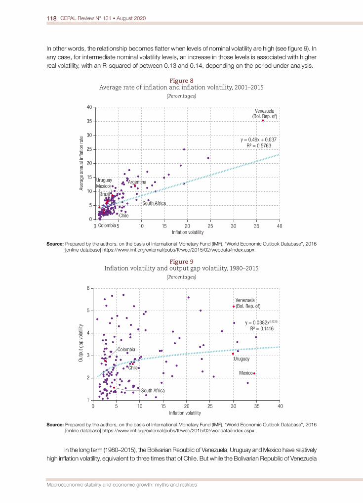
Between 2001 and 2015, most Latin American economies had average inflation rates of less than 10% (see figure 8). The exceptions are the Bolivarian Republic of Venezuela, with average annual inflation of almost 35% and high volatility, and Argentina, with an average annual inflation rate of just over 10%. Nevertheless, Argentina has an average rate of inflation and inflation volatility that are twice that of Brazil, Chile and Colombia, while the inflation rate and inflation volatility of the Bolivarian Republic of Venezuela are more than seven times that average. Uruguay and Brazil appear to have relatively low inflation volatility in relation to their average inflation rate. In contrast, Chile and Colombia have much lower inflation rates, but their volatility is relatively similar to the aforementioned countries. The Bolivarian Republic of Venezuela and Argentina have average inflation rates as well as clearly higher volatility, which separate them from the cohort, as well as from the rest of the Latin American countries.

Fact No. 3: Higher nominal volatility in general is associated with greater real volatility

Another interesting fact is that inflation volatility is not merely a harmless or inconsequential nominal volatility. It is also related to real volatility or output gap volatility. It is not as strong a relationship as that between inflation volatility and the average inflation rate; in fact, the relationship between inflation volatility and output gap volatility is nonlinear and real volatility decreases when levels of nominal volatility are high.5

5 Real volatility is calculated as the standard deviation of the output gap. Trend GDP is a seven-year average, centered on the fourth year.



In other words, the relationship becomes flatter when levels of nominal volatility are high (see figure 9). In any case, for intermediate nominal volatility levels, an increase in those levels is associated with higher real volatility, with an R-squared of between 0.13 and 0.14, depending on the period under analysis.

Figure 8 Average rate of inflation and inflation volatility, 2001–2015

(Percentages)

Argentina

Colombia

Uruguay

0

5

10

15

20

25

30

35

40


Aver

age

annu

al in

flatio

n ra

te y = 0.49x + 0.037R² = 0.5763


Brazil

Mexico

South Africa

Chile


Figure 9 Inflation volatility and output gap volatility, 1980–2015

(Percentages)

ChileMexico

South Africa

Colombia

Uruguay


1

2

3

4

5

6


Out

put g

ap v

olat

ility y = 0.0382x0.1325

R² = 0.1416


In the long term (1980–2015), the Bolivarian Republic of Venezuela, Uruguay and Mexico have relatively high inflation volatility, equivalent to three times that of Chile. But while the Bolivarian Republic of Venezuela



has a real or output gap volatility equivalent to more than twice that of Chile, Uruguay’s is barely 30% higher and Mexico’s is similar or even lower (see figure 9).6 This indicates that there are other factors or variables that also contribute to real volatility, as will be discussed below.

For the period 2001–2015, the positive correlation between nominal and real volatility is also true. In this regard, the nominal and real volatility in the Bolivarian Republic of Venezuela are noteworthy, given that they are much higher than that of the rest of the region’s countries during this period (see figure 10). The nominal volatility of the Bolivarian Republic of Venezuela is equivalent to more than seven times that of Chile, while its real volatility is equivalent to three times that of Chile in the period 2001–2015. The nominal and real volatility of Argentina are also high, more than twice those of Chile; in the case of Uruguay, the nominal volatility is similar to that of Chile, but its real volatility is 50% higher. Evidence suggests that output gap volatility is positively correlated with inflation volatility, although the latter does not have a unique or determinant effect.

Figure 10 Inflation volatility and output gap volatility, 2001-2015

(Percentages)

Argentina

BrazilColombia Chile

South Africa

Mexico

Uruguay


y = 0.0538x0.2778

R² = 0.1368

0

1

2

3

4

5

6


Out

put g

ap v

olat

ility


5. External and real volatility

It can be hypothesized that the growth problem in many emerging economies is one of external resource constraints; if they were able to finance large current account deficits it would encourage investment and boost GDP growth rates. This creates the myth that external capital inflows would stimulate growth.

Myth No. 3: Strong capital inflows that finance large current account deficits stimulate growth

Unfortunately, massive capital inflows do not always finance profitable investments and their reversals often lead to balance-of-payments crises with the usual negative effects on the financial system and on growth in economic activity and employment. In several articles, Calvo correlated balance-of-payments

6 Inflation volatility in Argentina and Brazil was so high that they do not appear on the graph —the scale of which has a maximum of 40%—, owing to periods of hyperinflation in the twentieth century.



crises to sudden stops in capital inflows, stressing the importance of fiscal institutions and public debt in avoiding this source of instability (Calvo, 2003). Edwards (2002 and 2004) also produced various papers that focus on the costs of maintaining high external debts that lead to current account reversals, whereby large deficit episodes are followed by more or less abrupt adjustments that produce transient effects on growth and increase real volatility. Furthermore, Edwards points out that, in general, current account reversals are linked to sudden stops of capital inflows.

Several other authors have also analysed the phenomena associated with external stability, including Milesi-Ferretti and Razin (1998), who examine which factors help to predict current account reversals and how these events affect a large number of variables relevant to macroeconomic stability. Thus, low reserves and external factors, such as unfavourable terms of trade or high interest rates in industrialized economies, often trigger sharp current account reversals, starting from a high deficit level, especially in developing countries. However, according to Milesi-Ferretti and Razin, the effects of reversals on long-term growth are not as clear because there are other factors that also influence the post-reversal performance. Thus, high and stable rates of saving and investment, financial development, low inflation rates and good economic policy can enable countries to emerge from current account reversals with even higher growth rates than those experienced before the reversal. Conversely, without these factors, the effects of reversals on growth can be more profound and long-lasting. Last but not least, countries with more flexible exchange rate regimes are better able to adjust to current account reversals than those with fixed exchange rates. They can also achieve a better post-crisis macroeconomic performance. In addition, openness and financial development are important issues when analysing reversals. Those countries that allow the free movement of capital and have no internal liquidity restrictions are able to better cope with these events.

Current account reversals (REV(CA)) are basically changes in the moving average of the current account balance (CAB) expressed as a percentage of GDP (CA).7 Thus, when economies’ current account deficits widen this produces a negative reversal first and then, when it is corrected, a positive reversal. A current account reversal is defined by taking the anticipated and lagged three-year moving averages of the current account balance, expressed as a percentage of GDP. The difference between the two is the indicator of reversals. If it is positive, it indicates a correction or the end of a deficit period; if it is negative, it indicates the opposite, that the deficit is widening. The literature examines some criteria that must be met for the change in the current account balance to be considered a reversal, including that the average reduction in the current account deficit must be at least 3 percentage points of annual GDP; that the deficit must be reduced by at least one third with respect to the deficit or surplus before the event; and, third, that the sign indicates whether it is a reversal from a deficit or a surplus. We then define the current account reversal (REV(CA)) as the difference between the average current account balance for the three-years after the event (t+j) and the average balance for the previous three-years (t-i), where j and i range from 1 to 3. The current account balance is measured as a percentage of GDP.

REV(CA)t=

3j = 02 CAt + j/

-3

i =13 CAt

CAt = CABt /GDPt

-1/

There is a non-linear relationship between average current account reversals and output gap volatility in the period 1980–2015. Thus, output gap volatility is minimal when the reversal is non-existent, tends to zero or is slightly positive (see figure 11). Volatility increases when the absolute value of the reversal is higher, but the effect is small and asymmetrical, weighted towards negative reversals. An increase in the average current account reversal from 0% to 2% of GDP increases output gap volatility by 0.5 percentage points; but a fall in the current account reversal from 0% to -2% of GDP increases output gap volatility by 1.5 percentage points.

7 Current account balances expressed as percentages of GDP were obtained from the World Economic Outlook database (IMF, 2016).



Figure 11 Output gap volatility and current account reversals as a percentage of GDP, 1980–2015

(Percentages)

Argentina

Brazil ChileMexico

South Africa

ColombiaUruguay


0

1

2

3

4

5

6

-2.0 -1.5 -1.0 -0.5 0 0.5 1.0 1.5 2.0Current account reversals as a percentage of GDP

Out

put g

ap v

olat

ility

y = -5978.9x4-137.18x

3+ 33.072x

2- 0.1807x + 0.0278

R² = 0.2365



If, instead of focusing on the average current account reversal, the analysis focuses on its volatility, the relationship between external instability and real instability is much more evident. There is a significant positive correlation between the volatility of the current account reversal and output gap volatility. According to the estimated norm, an increase in the volatility of the current account reversal from 2% to 4% increases output gap volatility from 1.8% to 2.5%. The relationship is nonlinear and the effect on real volatility is smaller for higher levels of external volatility, but in any case the R-squared exceeds 0.32.

Fact No. 4: Current account reversals are associated with higher real volatility

For some Latin American economies, current account reversals have not been the main source of real volatility in the last 30 years, but for others, the volatility of reversals, or external volatility, comes very close to explaining output gap volatility (see figure 12). While the volatility of current account reversals in the period 1980–2015 for some countries is between 2% and 4% (Uruguay, Brazil, Chile, Mexico and Argentina), others register between 6% and 8% (Colombia and the Bolivarian Republic of Venezuela). Most notably, almost all of them are in a low volatility range for current account reversals and, with the exception of the Bolivarian Republic of Venezuela, below the global average.

At the same time, these economies have very different output gap volatilities, ranging from the Bolivarian Republic of Venezuela and Argentina, with values of over 4% and above the global average for real volatility, to Mexico and Brazil, with values close to 2%, well below the global average for real volatility. Furthermore, while output gap volatility in Brazil, Mexico, Chile and Colombia is close to the norm and is therefore “explained” by the volatility of their current account reversals, output gap volatility in Uruguay, Argentina and the Bolivarian Republic of Venezuela is much higher than the norm, indicating that there are other factors that explain the real volatility in these countries. From the outset, these last three countries had significant levels of nominal volatility, from which it could be concluded that external volatility and nominal volatility added to real volatility. This is certainly an interesting hypothesis to explore with more sophisticated econometric methods.



Figure 12 Output gap volatility and the volatility of current account reversals, 1980–2015

(Percentages)

Argentina

Mexico

ChileBrazil

South Africa

Colombia

Uruguay


0

1

2

3

4

5

6

0 2 4 6 8 10 12 14 16 18 20

Volatility of current account reversals as a percentage of GDP

Out

put g

ap v

olat

ility

y = 0.1109x 0.466

R² = 0.3188



III. Econometric methodology and results

The relationships that we have been able to establish on the basis of data from all the countries, aggregated over different periods of time, do not allow us to test hypotheses and are instead descriptive of the situation. The econometric panel data methodology allows relevant parameters to be estimated and provides evidence of their significance, which may possibly support the hypotheses put forward in section II. We will estimate different relationships using data from the World Economic Outlook database, which provided us with a sample of annual data for 189 countries ranging from 1984 to 2015 (IMF, 2016).

1. Growth and volatility

The data used correspond to the five-year moving average for GDP growth and, as in the first models, volatility, such as output gap volatility (VolGDP), is also measured in five-year windows. The following equation has been defined, where volatility explains growth:

dlogGDPi,t (5) = η+α1 VolGDPi,t + ui,t

The simplicity of the equation should not be confused with the importance of the result. It seeks to show the nature of the relationship between output gap volatility and GDP growth. Two equations will be estimated, one for all the countries in the sample and the second for countries with output gap volatility of less than 50%. The results are shown in table 1.



Table 1 GDP growth and output gap volatility, sample of 189 countries, 1984–2019

Variables(1)

VolGDPLGDPP5

(2)VolGDPL50

GDPP5VolGDP -0.126*** -0.212***

(0.00914) (0.0134)

Constant 7.619*** 8.468***

(0.261) (0.261)

Fixed effect (year) No No

Fixed effect (country) No No

Observations 6 237 6 138

Number of countries 189 189

Source: Prepared by the authors.Note: Standard errors are shown in parentheses. *** p<0.01; ** p<0.05; * p<0.1.

As expected, output gap volatility has a negative and statistically significant impact at 1% on trend GDP growth. It is interesting to note that the effect of volatility on growth is equally negative and significant, but of much greater absolute value, when extreme or atypical cases (those countries with excessive and persistent volatilities), are removed from the sample. This result is consistent with the preliminary information presented in the previous section.

2. Interaction between threshold and volatility

It has been proposed to incorporate additional models to include effects on levels of and with respect to thresholds for the relationship studied between GDP growth and output gap volatility. The data used correspond to the five-year moving average for GDP growth and, as in the first models, output gap volatility is also measured in five-year windows, represented by VolGDPi,t; additionally, a dummy variable is incorporated, represented by DVolGDPi,t, which takes a value of 1 for countries with an output gap volatility greater than 50%, and an interaction between this variable and VolGDPi,t. The models to be estimated are:

GDPi,t(5) = η + α1 VolGDPi,t + α2 DVolGDPi,t+ α3 VolGDPi,t∙ DVolGDPi,t + ui,t

GDPi,t (5)= η + δt + α1 VolGDPi,t + α2 DVolGDPi,t + α3 VolGDPi,t∙ DVolGDPi,t + ui,t

GDPi,t (5)= η + δt + δi + α1 VolGDPi,t+ α2 DVolGDPi,t + α3 VolGDPi,t∙ DVolGDPi,t + ui,t

When calculating the aforementioned relationships, it is found that the results of the three equations demonstrate the same correlations, whereby output gap volatility generates less growth. Moreover, this negative effect will be more pronounced the more fixed effects are incorporated into the estimate. In turn, volatility above the 50% threshold produce an abrupt fall in growth rates; that is, countries with very high volatility grow little or undoubtedly suffer from recessions. Meanwhile, the interactive variable (VolGDPDVolGDP) shows that, for certain volatility points, combined with persistently high volatilities, higher growth is generated; this can be explained by countries’ special circumstances, such as that of the Syrian Arab Republic, which years before the sub-prime crisis had very high negative growth, while after the crisis it recovered all or part of its lost growth (see table 2).



Table 2 GDP growth and output gap volatility, effects on levels and with respect

to thresholds, sample of 189 countries, 1984–2019

Variables (1)dlogGDPP5

(2)dlogGDPP5

(3)dlogGDPP5

VolGDP -0.212*** -0.241*** -0.283***

(0.0147) (0.0139) (0.0144)

DVolGDP -14.48*** -14.76*** -15.39***

(2.245) (2.008) (2.001)

VolGDPDVolGDP 0.272*** 0.291*** 0.323***

(0.0300) (0.0271) (0.0274)

Constant 8.488*** 2.897*** 5.908***

(0.283) (0.621) (1.828)

Fixed effect (year) No Yes Yes

Fixed effect (country) No No Yes

Observations 6 237 6 237 6 237

Number of countries 189 189 189


3. Nominal and real volatility

To estimate how growth behaves around nominal and real volatilities, we used a sample consisting of 189 countries in total and 186 countries when only those countries with less than 50% of inflation volatility are considered, with data from 1984 to 2019. The data used correspond to the five-year moving average for GDP growth and, as in the first models, volatility, such as output gap volatility, is also measured in five-year windows. The following model was determined:

VolInfi,t = η + α1 Infi,t(5) + ui,t

The model estimations were then carried out twice, once for all the countries and once omitting countries with inflation volatility above 50% (see table 3).

Table 3 Panel regression for inflation and inflation volatility,

sample of 189 countries, 1984–2019

Variables(1)

VolINFLVolInf

(2)VolINFL50

VolInfInfP5 0.102*** 0.0493***

(0.000887) (0.00106)

Constant 1.798e+09* 3.747***

(1.021e+09) (0.403)

Fixed effect (year) No No

Fixed effect (country) No No






From column (1) of table 3 it can be seen that the model provides statistically significant estimates that show that inflation volatility is greater when the inflation rate is higher. With regard to the estimate for those countries with volatility below 50%, the effect is even more evident and decisive; in general, the average volatility is 3.7% and each extra percentage point of inflation generates an additional 0.049% of volatility.

It is possible to try to improve the relationship between real volatility and nominal volatility by introducing distinctions with respect to inflation levels.

ln(VolGDPi,t ) = η+δi + δt + α1 ln(VolInfi,t ) + α2 D(Infi,t (5) > 10%) + ui,t

The results indicate that the increase in inflation volatility generates positive and significant effects on output gap volatility. However, the constant is lower for high volatility levels. Thus, the results of the panel estimation reproduce what was observed by crossing the variables (see table 4).

Table 4 Panel regression for output gap volatility and inflation volatility


Variables(1)

EQ2ln(VolGDP)

Ln(VolInf) 0.0389***

(0.00776)

DInf -0.545***

(0.0420)

Constant 2.110***

(0.156)

Fixed effect (year) Yes

Fixed effect (country) Yes

Observations 6 185

Number of countries 189


In order to explore further the empirical correlation between nominal and real volatilities, we decided to use the following polynomial models to estimate this relationship, three of them without the dummy variable that indicates output gap volatility over 50%, and another that includes it (it should also be noted that the estimate has only been made for countries with inflation volatility under 50%):

VolGDPi,t = η + δt+α1VolInfi,t + α2VolInfi,t2+α3VolInfi,t

3 + ui,t

VolGDPi,t = η + δi + α1VolInfi,t + α2VolInfi,t2 + α3VolInfi,t

3 + ui,t

VolGDPi,t = η + δt + δi + α1VolInfi,t + α2VolInfi,t 2 + α3VolInfi,t

3 + ui,t

VolGDPi,t = η + δt + δi + α1VolInfi,t + α2VolInfi,t 2 + α3VolInfi,t

3 + α4DVolGDP50i,t + ui,t

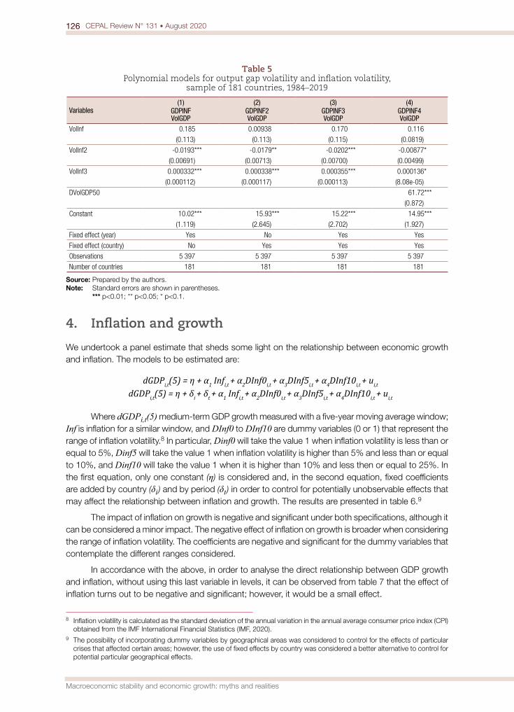
The results of the estimations are presented in table 5.

All models use the third degree polynomials for inflation volatility as explanatory variables. In particular, the second and third degree polynomials appear to have greater statistical significance than the first degree component, which may be due to the large variance of the data and the use of fixed effects models that may be capturing variations in inflation volatility. As in the previous case, the marginal effect of inflation volatility on output gap volatility is positive for inflation volatility levels below 5% and above 35%. That is to say, for both low and high inflation volatility, the marginal effect of inflation volatility on output gap volatility is clearly positive and statistically significant.



Table 5 Polynomial models for output gap volatility and inflation volatility,


Variables(1)

GDPINFVolGDP

(2)GDPINF2VolGDP

(3)GDPINF3VolGDP

(4)GDPINF4VolGDP

VolInf 0.185 0.00938 0.170 0.116

(0.113) (0.113) (0.115) (0.0819)

VolInf2 -0.0193*** -0.0179** -0.0202*** -0.00877*

(0.00691) (0.00713) (0.00700) (0.00499)

VolInf3 0.000332*** 0.000338*** 0.000355*** 0.000136*

(0.000112) (0.000117) (0.000113) (8.08e-05)

DVolGDP50 61.72***

(0.872)

Constant 10.02*** 15.93*** 15.22*** 14.95***

(1.119) (2.645) (2.702) (1.927)

Fixed effect (year) Yes No Yes Yes

Fixed effect (country) No Yes Yes Yes

Observations 5 397 5 397 5 397 5 397

Number of countries 181 181 181 181


4. Inflation and growth

We undertook a panel estimate that sheds some light on the relationship between economic growth and inflation. The models to be estimated are:

dGDPi,t(5) = η + α1 Infi,t + α2DInf0i,t + α3DInf5i,t + α4DInf10i,t + ui,t

dGDPi,t(5) = η + δi + δt + α1 Infi,t + α2DInf0i,t + α3DInf5i,t + α4DInf10i,t + ui,t

Where dGDPi,t(5) medium-term GDP growth measured with a five-year moving average window; Inf is inflation for a similar window, and DInf0 to DInf10 are dummy variables (0 or 1) that represent the range of inflation volatility.8 In particular, Dinf0 will take the value 1 when inflation volatility is less than or equal to 5%, Dinf5 will take the value 1 when inflation volatility is higher than 5% and less than or equal to 10%, and Dinf10 will take the value 1 when it is higher than 10% and less then or equal to 25%. In the first equation, only one constant (η) is considered and, in the second equation, fixed coefficients are added by country (δi ) and by period (δt ) in order to control for potentially unobservable effects that may affect the relationship between inflation and growth. The results are presented in table 6.9

The impact of inflation on growth is negative and significant under both specifications, although it can be considered a minor impact. The negative effect of inflation on growth is broader when considering the range of inflation volatility. The coefficients are negative and significant for the dummy variables that contemplate the different ranges considered.

In accordance with the above, in order to analyse the direct relationship between GDP growth and inflation, without using this last variable in levels, it can be observed from table 7 that the effect of inflation turns out to be negative and significant; however, it would be a small effect.

8 Inflation volatility is calculated as the standard deviation of the annual variation in the annual average consumer price index (CPI) obtained from the IMF International Financial Statistics (IMF, 2020).

9 The possibility of incorporating dummy variables by geographical areas was considered to control for the effects of particular crises that affected certain areas; however, the use of fixed effects by country was considered a better alternative to control for potential particular geographical effects.



Table 6 Panel regressions for GDP growth and the inflation rate,


Variables (1)dGDPP5

(2)dGDPP5

InfP5 -0.00428*** -0.00383***

(0.00139) (0.00141)

DInf0 -0.559*** -0.613***

(0.133) (0.135)

DInfl5 -0.349** -0.392***

(0.144) (0.146)

DInfl10 -0.272** -0.275**

(0.107) (0.108)

Constant 2.252*** 2.197***

(0.118) (0.111)


R squared 0.009



Table 7 Panel regressions for GDP growth and the inflation rate,


Variables(1)

C1b1GDPP5

(2)C1b2

GDPP5InfP5 -2.31e-13* -2.71e-13**

(1.35e-13) (1.36e-13)

Constant 6.303*** 3.554*

(0.282) (2.091)

Fixed effect (year) No Yes

Fixed effect (country) No Yes




It was then, in accordance with the findings of Khan and Senhadji (2001), deemed advantageous to estimate the effect of certain inflation threshold, in order to show that inflation higher than that range has negative effects on growth, while an inflation rate lower than that range might not be harmful. Thus, GDP growth is estimated based on an interactive variable D(Inf > 10%), which will take the value 1 if inflation exceeds 10% in the five-year moving average, and will interact with the level of inflation. Thus, we seek to find a nonlinear relationship, which indicates how large the effect is, depending on how much further away inflation is from 10%. So, the equation to be estimated is:

dGDPi,t(5) = η + δi + δt + α1 Infi,t (5) × D(Infi,t (5) > 10%) + ui,t

The results are presented in table 8.

It can be seen that the negative effect of inflation over a certain range on growth is small but significant. The effect is negative for countries with inflation above 10% and this effect increases with higher inflation rates. Meanwhile, in countries with inflation rates below 10%, inflation does not affect GDP growth, which averages 3.5%.



Table 8 Panel regressions for GDP growth and inflation from the 10% threshold,


Variables(1)

EQ0dGDP5

InfDInf10 -2.71e-13**

(1.36e-13)

Constant 3.554*

(2.091)



Observations 6 239



5. Disinflation and its real costs

To observe the effects that the acceleration of inflation has on the speed of growth, the equations presented below were estimated, in which the variable dGDPi,t (5) reflects the speed of growth, while dInfi,t (5) reflects the acceleration of inflation:

dGDPi,t (5) = η + δi + δt + α1dInfi,t(5) + α2 Infi,t(5) × D(Infi,t-1(5) > 10%) + ui,t

dGDPi,t (5) = η + δi + δt + α1dInfi,t(5) × D(Infi,t-1(5) > 10%) + ui,t

The results of this estimate, based on the interaction term, should be interpreted as the acceleration effect in countries that have inflation levels consistently above 10% (see table 9).

Table 9 Panel regressions for the acceleration of GDP growth and of inflation,


Variables(1)

EQ1dGDPP5

(2)EQ1b

dGDPP5dInfP5 1.32e-12

(1.86e-12)

InfDInf2 -1.07e-13

(1.18e-13)

dInfDinf2 1.73e-13

(1.36e-12)

Constant -0.00584 -0.000639

(1.341) (1.341)




A review of the results shows that there is no apparent relationship between the variables; that is to say, the inflation slowdown does not have a statistically significant impact on the growth slowdown for different specifications.



6. External and real volatility

Based on the revised stylized facts presented above, it is interesting to see how GDP growth volatility behaves with respect to current account volatility and their interaction in conjunction with the inflation threshold.

ln(VolGDPi,t ) = η + δi + δt + α1 ln(VolCABi,t ) + α2ln(VolCABi,t) D(Infi,t(5) > 10%) + ui,t


Table 10 GDP growth volatility and current account volatility,


Variables(1)

EQ3ln(VolGDP)

Ln(VolCAB) 0.0523***

(0.0146)

VolCABDInf 0.102***

(0.00991)

Constant 2.127***

(0.157)



Observations 6 164



Table 10 shows that those countries that experienced current account volatility see this transferred to GDP growth volatility. The significant positive coefficient of the variable Ln(VolCAB) indicates that a 1% increase in current account volatility escalates GDP growth volatility by approximately 0.05%. Moreover, the real volatility of countries with inflation rates above 10% was affected to a greater extent by changes in current account volatility, probably because macroeconomic stability was already weakened by nominal volatility to such an extent that the additional effect of external volatility was more damaging than it was in economies with nominal stability.

In order to analyse whether there are additive effects of nominal and external volatilities on real volatility, an equation was calculated that includes the relationship between GDP growth volatility, inflation volatility and current account volatility. The equation is as follows:

ln(VolGDPi,t ) = η + δi + δt + α1 ln(VolInfi,t ) + α2 ln(VolCABi,t )

+ α3 ln(VolCABi,t )D(Infi,t(5) > 10%) + ui,t


The results show that the relationships are all significant and that inflation volatility brings about greater GDP growth volatility, although the effect is small. Meanwhile, higher current account volatility also contributes positively to output gap volatility. Lastly, current account volatility combined with inflation levels above 10% also contributes positively, and quite significantly, to output gap volatility.



Table 11 GDP growth volatility, inflation volatility and current account volatility,


Variables(1)

EQ4ln(VolGDP)

Ln(VolInf) 0.0223***

(0.00767)

Ln(VolCAB) 0.0315**

(0.0157)

Ln(VolCAB)DInf 0.117***

(0.0113)

Constant 2.069***

(0.158)



Observations 6 119



IV. Conclusions and policy implications

Macroeconomic stability, in its various dimensions —nominal, real and external—, is in itself desirable because it implies less uncertainty for risk-averse economic agents. Even so, there is a firm belief that macroeconomic instability, in the form of inflation, a sizeable external deficit or a large positive GDP gap with the consequent overutilization of resources, could boost economic growth. Even if this were the case, it is highly questionable whether this would improve well-being, because expansionary policies increase real volatility, so the burden of proof falls on the proponents of macroeconomic instability. For destabilizing expansionary policies to contribute to greater social well-being, they would have to exert such a positive impact on GDP growth that it would be more than sufficient to offset the negative effects wrought by uncertainty and volatility. Consequently, if it can be shown that real macroeconomic volatility does not stimulate growth, this is sufficient to show that instability does not contribute positively to well-being.

We have been able to show in this paper that medium-term or trend GDP growth is negatively associated with output gap volatility, defined as logarithmic deviations between GDP and its trend. We can interpret this as meaning that overzealous, procyclical demand policies that force subsequent corrective action not only increase output gap volatility, but also slow the trend growth rate significantly. The available evidence suggests that higher real volatility is correlated with a lower rate of GDP growth, so macro policies should be countercyclical and seek to reduce volatility.

We have explored the relationship between macroeconomic stability in its various dimensions and economic growth. The main conclusion is that there is no basis for the idea that the loss of macroeconomic stability contributes positively to growth. Rather, the available information suggests that expansionary policies, which lead to high inflation or unsustainable external current account balances that end in reversals, are detrimental to growth.

Inflation is seen in some circles as a kind of growth facilitator and in many situations there are those who call for “a little more inflation to boost growth”. In a context of rigid downward pricing there is some analytical basis for this argument, but not to a great extent. At first sight, long-term data tend to support the hypothesis of no correlation between growth and inflation.

Thus, a “little bit more inflation” creates more nominal and real volatility instead of boosting GDP growth. The relationship between the average rate of inflation and inflation volatility is clearly positive and



quite strong in the long and medium term. In addition, inflation volatility, or nominal volatility, is positively associated with output gap volatility, or real volatility, although it does not have a unique or determinant effect. An increase in inflation volatility escalates output gap volatility; the relationship is positive, but nonlinear and the response of real volatility decreases for very high levels of inflation and nominal volatility.

In a slightly more detailed analysis, we tried to identify a change in the relationship between growth and inflation, beyond certain thresholds of the inflation rate. Our results replicate those of Khan and Senhadji (2001), and the inflation threshold above which it would have a negative effect on trend GDP growth would be between 11% and 12% per year for developing countries. Lower inflation has no effect on growth, although there may be a minimum threshold of zero or negative inflation, under which the relationship between inflation and growth becomes positive. It was not possible to verify this, owing to data limitations, as the dataset did not contain many observations with zero or negative inflation rates.

Although high inflation can have considerable costs, when given the choice of stabilizing prices or reducing inflation, there are those who point to the real costs in terms of GDP growth of pursuing disinflation. But even if the ongoing benefits of stabilization are ignored, there is no clear evidence that the real costs of that process will persist over the medium term. For 15-year periods, the correlation between the acceleration of inflation and of growth is tenuous, and consistently negative, so the information indicates that many countries have been able to achieve nominal stabilization without a further slowdown in growth. The costs of stabilization are short-term and largely avoidable if an appropriate strategy is adopted, which includes pursuing disinflation only at high or moderately high inflation rates and never at very low rates of inflation, and regulating the pace of disinflation with gradual but sustained cuts. Similarly, it is preferable to do so with exchange rate flexibility in order to avoid real appreciation of the domestic currency and with independent local monetary authorities, although it was not possible to support these findings with the data that was available.

Real volatility also has other origins, such as those related to external and internal shocks that affect the balance-of-payments current account. Massive inflows of foreign capital tend to produce a spending and output boom, financed by a current account deficit.10 But in the long run, this often ends in a reversal of the current account balance, with the usual negative effects on the financial system, economic activity and employment. Available information on the effects of current account reversals on medium-term growth indicates that these depend on many other factors that affect the post-reversal performance, but a much clearer and more evident direct correlation between external and real volatilities can be identified.

There is a positive nonlinear relationship between average current account reversals and output gap volatility in the period 1980–2015. Thus, output gap volatility is minimal when the current account reversal is non-existent or slightly positive, but real volatility increases when the absolute value of the reversal is higher. If, instead of analysing the average current account reversal, we focus on its volatility, the relationship between external instability and real instability is much more evident. There is a positive correlation between the volatility of the current account reversal and output gap volatility. This relationship is nonlinear and the effect on real volatility is smaller for higher levels of external volatility. For some Latin American economies, the volatility of current account reversals comes very close to explaining output gap volatility, but for others current account reversals do not seem to be a major source of real volatility.

The econometric analysis carried out has allowed us to verify that countries with higher real volatility tend to grow less than those with a less pronounced cycle. We have also been able to show that both high inflation rates and frequent current account reversals contribute significantly to real volatility and macroeconomic instability. As a result, countries that tend to have inflation accelerations and whose current account deficits widen precipitously, generally fail to increase their trend growth rate. Conversely, greater nominal, external and real volatility ends up acting as a brake on growth.

The policy implications of these results are obvious. It is important to promote nominal stability by maintaining low, single-digit, stable inflation. It is also important to adopt countercyclical aggregate

10 See, for example, the situation in Chile before the Asian financial crisis, outlined in Le Fort and Lehmann (2003).



demand policies, such as monetary and fiscal policies, by reducing real volatility. Moreover, it is advisable to take steps to prevent the balance of the balance-of-payments current account from being subject to large reversals, which means avoiding the procyclical effect on domestic demand of strong capital inflows and large currency appreciations. This may require the implementation of various instruments, including floating exchange rates, a credible nominal anchor such as inflation targeting and prudential financial regulations, as well as the adoption of a countercyclical fiscal policy. However, the detail of these policy designs goes far beyond the scope of this paper, the available data and the models that were developed. They are left for a future endeavour.

BibliographyBarro, R. (1995), “Inflation and economic growth”, NBER Working Paper, No. 5326, Cambridge, National

Bureau of Economic Research (NBER), October.Blanchard, O. and J. Simon (2001), “The long and large decline in U.S. output volatility”, Brookings Papers

on Economic Activity, No. 1.Bruno, M. and W. Easterly (1998), “Inflation crises and long-run growth”, Journal of Monetary Economics,

vol. 41, No. 1, February.Calvo, G. (2003), “Explaining sudden stops, growth collapse and BOP crises: the case of distortionary output

taxes”, NBER Working Paper, No. 9864, Cambridge, National Bureau of Economic Research (NBER), July. Calvo, G. and C. Végh (1999), “Inflation stabilization and BOP crises in developing countries”, Handbook of

Macroeconomics, vol. 1C, J. Taylor and M. Woodford (eds.), Amsterdam, North-Holland.Calvo, G., O. Celasun and M. Kumhof (2003), “Inflation inertia and credible disinflation- the open economy

case”, NBER Working Paper, No. 9557, Cambridge, National Bureau of Economic Research (NBER), March.Christoffersen, P. and P. Doyle (1998), “From inflation to growth: eight years of transition”, IMF Working Paper,

No. 98/100, Washington, D.C., International Monetary Fund (IMF), July. Edwards, S. (2004), “Thirty years of current account imbalances, current account reversals, and sudden

stops”, IMF Staff Papers, vol. 51, special issue, Washington, D.C., Palgrave Macmillan. (2002), “Does the current account matter?”, Preventing currency crises in emerging markets, S. Edwards

and J. Frankel (eds.), Chicago, University of Chicago Press.Faria, J. and F. Carneiro (2001), “Does high inflation affect growth in the long and short-run?”, Journal of

Applied Economics, vol. 4, No. 1. Ghosh, A. and P. Steven (1998), “Warning! Inflation may be harmful to your growth”, IMF Staff Papers, vol. 45,

No. 4, Washington, D.C., Palgrave Macmillan. IMF (International Monetary Fund) (2020), “International Financial Statistics” [online database] https://data.

imf.org/?sk=4C514D48-B6BA-49ED-8AB9-52B0C1A0179B&sId=1409151240976. (2016), “World Economic Outlook Database” [online database] https://www.imf.org/external/pubs/ft/

weo/2015/02/weodata/index.aspx.Khan, M. and A. Senhadji (2001), “Threshold effects in the relationship between inflation and growth”, IMF

Staff Papers, vol. 48, No. 1, Washington, D.C., Palgrave Macmillan.Le Fort, G. and S. Lehmann (2003), “The unremunerated reserve requirement and net capital flows: Chile in

the 1990s”, CEPAL Review, No. 81 (LC/G.2216-P), Santiago, Economic Commission for Latin America and the Caribbean (ECLAC), December.

Le Fort, G., B. Gallardo and F. Bustamante (2017), “Estabilidad macroeconómica y crecimiento económico: mitos y realidades”, Documento de Trabajo, No. 456, Santiago, University of Chile, November.

Loungani, P. and N. Sheets (1997), “Central bank independence, inflation and growth in transition economies”, Journal of Money, Credit, and Banking, vol. 29, No. 3.

Milesi-Ferretti, G. and A. Razin (1998), “Current account reversals and currency crises: empirical regularities”, NBER Working Paper, No. 6620, Cambridge, National Bureau of Economic Research (NBER), June.

Sidrauski, M. (1967), “Rational choice and patterns of growth in a monetary economy”, The American Economic Review, vol. 57, No. 2, May.

Végh, C. (1992), “Stopping high inflation: an analytical overview”, IMF Staff Papers, vol. 39, No. 3, Washington, D.C., Palgrave Macmillan, September.

Zarnowitz, V. and G. Moore (1986), “Major changes in cyclical behavior”, The American Business Cycle: Continuity and Change, R. Gordon (ed.), Chicago, University of Chicago Press.

Macroeconomic stability and economic growth - Repositorio ...

Documents

Transcript of Macroeconomic stability and economic growth - Repositorio ...