Microeconomic Uncertainty and Macroeconomic Indeterminacy1

Jean-Francois Fagnart

THEMA, Universite de Cergy-Pontoise

and

Henri R. Sneessens

IRES, Universite catholique de Louvain, and Universite catholique de Lille

April 2001

1We are most grateful to Jorge Duran for his detailed and stimulating comments on an earlier version

of the paper. We also wish to thank (without implicating) R.Boucekkine, D. de la Croix and J.H.Dreze

for their thoughtful questions and comments. Financial support from the IAP IV and ARC programmes

is gratefully acknowledged.

Abstract

We construct a stylised intertemporal macroeconomic model to illustrate how the combination of

decentralised trading and microeconomic uncertainty can generate coordination problems and

indeterminacy of the macroeconomic equilibrium. With a competitive labour market and a

fixed labour supply,the range of equilibria depends mainly on the variance of the idiosyncratic

shocks and may thus remain fairly narrow . The situation is different when there is imperfect

competition on the labour market. The existence of real rigidities is apt to considerably increase

the size of the interval of indeterminacy, for a given variance of the shocks.

Keywords: indeterminacy, non-Walrasian economy, equilibrium unemployment, coordination,

continuum of equilibria

JEL classification: E10, E24

1 Introduction

Business cycle analysts often associate the success or failure of an economic recovery to in-

vestors and/or consumers expectations and degree of confidence. Subjective confidence effects

can hardly be discussed in standard Walrasian setups wherein the knowledge of the economy’s

“fundamentals” typically suffices to determine a unique equilibrium trajectory. It is well-known

that there is room for “animal spirits” to affect the macroeconomic outcome only if there are

market imperfections. This paper focuses on a market imperfection arising from the combina-

tion of decentralised trading and microeconomic uncertainty in an intertemporal setup. This

combination creates information problems between agents and can make the macroeconomic

equilibrium depend on agents’ expectations.

In an intertemporal perspective, decentralised trading implies that agents have to make decisions

that will commit them on a market (at least temporarily) while they are still uncertain about

their future trading opportunities. The simplest example is the choice of a productive capacity

under uncertainty about future purchase orders. In a Walrasian setup, such an uncertainty

may in the end have little macroeconomic implications, because (it is assumed that) there is

ex post full information about each other’s trading opportunities. The market works as if

there were a centralised market clearing device, which implies that all agents can realise all (ex

post) profitable transactions. If however agents do not enjoy such an amount of information,

the microeconomic uncertainty may create an information problem between buyers and sellers.

A firm may end up ex post with an excess productive capacity if it receives fewer purchase

orders than expected, or face a capacity shortage in the opposite case. The possibility of such

outcomes affects the firm’s investment decision and makes the optimal capital stock depend

on expectations about forthcoming orders. In such a non-Walrasian setup, expectations about

future trading opportunities may affect the actual level of transactions, and make low activity

levels result from low investments following from (self-fulfilling) pessimistic expectations.

Our objective is to formalise these intuitions in a model that departs as little as possible from a

standard Walrasian intertemporal macroeconomic model. To introduce the type of information

problem we have in mind, we distinguish final and intermediate goods producers. Intermediate

goods producers are all ex ante identical; they use labour and capital to produce an homoge-

neous good that is the sole input of final goods producers. Both types of firms operate under

perfect competition. We consider the case where uncertainty arises from the existence of purely

idiosyncratic technological shocks in intermediate firms. These idiosyncratic shocks imply het-

erogeneous employment and production decisions at the competitive prices and wages. In a

Walrasian world, final firms always buy a quantity of intermediate goods such that every inter-

mediate firm is always able to sell its optimal production level. This can occur in a decentralised

economy if final firms receive all the relevant information about every intermediate firm’s situ-

ation and can send purchase orders accordingly. In this case, the microeconomic heterogeneity

may have little or no macroeconomic implication. We want to depart slightly from this sce-

nario by analysing the case where final firms send purchase orders to intermediate firms without

knowing every intermediate firm’s optimal production level. The price of the homogeneous in-

termediate good fails to convey to buyers the relevant information about every intermediate

firm’s situation. An intermediate firm enjoying a good productivity shock may then receive

too few purchase orders, and vice-versa. The possibility of such outcomes makes the intermedi-

ate firms investment choice depend on expected forthcoming purchase orders. It is shown that

these expectation effects induce indeterminacy of the macroeconomic equilibrium, even with full

employment of a fixed labour supply. This indeterminacy is intrinsically linked to the informa-

tion problem between buyers and sellers induced by the microeconomic uncertainty. Without

idiosyncratic shocks, there is a unique equilibrium, which replicates the Walrasian outcome.

Our paper is related to an already vast literature aiming to understand under what circum-

stances multiple equilibria can occur in a decentralised economy. Those models have in common

the existence of a coordination failure due to some type of “externality” (physical or pecuniary1).

But they differ by the nature of the externality (technological interactions, demand externali-

ties, trading externalities) that is at the root of the coordination problem and generates multiple

equilibria. Hart (1982), Heller (1986), Kiyotaki (1988), Roberts (1987, 1989) and others rely on

multisectoral models with imperfect competition and “aggregate demand externalities” (in the

terminology of Blanchard-Kiyotaki (1987)). Diamond (1982) stresses the effects of decentralised

trading in an economy where the Walrasian auctioneer is replaced by a stochastic matching pro-

cess. Bryant (1983) emphasises imperfect information in a stylised model with complementary1For a discussion of these concepts, see Silvestre (1995).

2

intermediate goods and decentralised decision-making.

Our contribution shares many of the intuitions common to the above-mentioned papers. Our

model is different though in that it does not rely on imperfect competition nor on any physical

externality or technological complementarity. The model economy only departs from a Walrasian

one in the working of a competitive market (the intermediate goods one). This departure

would be inconsequential in a world with perfect information. Indeterminacy occurs because

the microeconomic uncertainty implies imperfect information between buyers and sellers. There

is then a continuum of equilibria that can be indexed by demand expectations. This means that

once a relatively pessimistic atmosphere has established itself, a unilateral change in expectations

is never profitable. It is only a coordinated change in expectations that can give intermediate

firms an incentive to invest more.

We also stress the possible interactions between the mechanism inducing indeterminacy and

the presence of real rigidities on the labour market. With a competitive labour market and

a fixed labour supply, we show that the range of equilibria depends mainly on the variance

of the idiosyncratic shocks. It may thus remain fairly narrow if the variance of these shocks

is itself small. The situation becomes totally different when there is imperfect competition

on the labour market. Because then both the employment rate and the capital stock change

with demand expectations, the existence of real rigidities is apt to considerably increase the

size of the interval of indeterminacy, for a given variance of the shocks. This result is in line

with Dreze (1997, 1999), who emphasises the possibility that, if some relative prices (like the

real wage) are downwardly rigid, underutilisation of resources (at prices compatible with full-

employment) may persist once established, reflecting pure coordination failure rather than price

distortions.

The rest of the paper is organised as follows. Section 2 is devoted to the description of behaviours

and equilibrium conditions in the Walrasian setup used as a benchmark case in the subsequent

sections. This framework is adapted in section 3 to the case of a non-Walrasian intermediate

goods market. Section 4 introduces imperfect competition on the labour market and assumes

that wages are set by a monopoly union. The main conclusions are summarised in section 5.

3

2 The Walrasian Economy

We first describe the Walrasian economy that will serve as a benchmark case for the rest of the

paper. We consider an economy with two types of firms, final goods producers and intermediate

goods producers. Intermediate good producers face a standard neoclassical technological con-

straint with two inputs (labour and capital), non-increasing returns to scale and idiosyncratic

productivity shocks. All intermediate goods are perfect substitutes in the production of a final

good. The latter uses no other input. We limit ourselves to the case where the idiosyncratic

uncertainty generates no macroeconomic uncertainty, which requires that all firms be ex ante

identical. We thus assume perfect foresight of all macro variables.

2.1 Behaviours

Intermediate Goods Producers

We assume a continuum of ex ante identical competitive firms, uniformly distributed over the

unit interval. In each firm, total factor productivity is random. With kt units of capital and `t

units of labour, a firm produces a quantity of output qt given by:

qt = θt f(kt, `t), (1)

where θt is a stochastic productivity shock, which is firm specific and observed at the beginning

of period t. f is concave and strictly increasing (fk, f` > 0, fkk, f`` < 0 and fk` > 0); it

exhibits non-increasing returns to scale. To further simplify the presentation, we assume that

the productivity shock can take only two values (low and high), the same for all firms. More

precisely:

θt =

θ− with probability π satisfying 0 < π < 1,

θ+ with probability 1− π,

(2)

and θ+ > θ− > 0. Given our assumptions on the distribution of θt, π represents in every period

both the probability that a given firm experiences a low productivity level θ− and the proportion

of firms experiencing such a low productivity level.

4

Every firm behaves competitively on all markets and thus takes the intermediate goods price pt,

the wage rate wt and the interest rate rt as given (the final good serves as numeraire).

We assume the following sequence of events and decisions. An investment made in t−1 becomes

productive in t. In period t − 1, each intermediate goods producer decides on the productive

capital stock of the next period (kt) without knowing the time t value of total factor productivity

θt. The period t employment and production decisions are only taken after the realised value of θt

has been observed. We analyse this sequence of decisions backwards, starting with employment

at given capital stock.

Optimal labour demand

Given a predetermined capital stock kt and a realised value of the shock, θt ∈ {θ−, θ+}, the

employment decision in period t is the solution of the following programme:

max`t

pt θt f(kt, `t) − wt `t.

Let us denote by `−t and q−t (resp. `+t and q+

t ) the optimal employment and output levels in a

firm where productivity is low (resp. high) in period t. The optimal employment level `±t must

be such that θ± f`(kt, `±t ) = wt/pt. This implies:

`±t = `(kt, ωt, θ±) and q±t = q(kt, ωt, θ

±) (3)

where ωt is the intermediate firm’s real labour cost in period t, i.e., ωt = wt/pt. Functions `

and q are increasing in both kt and θt and decreasing in ωt. Appendix 1 derives these functions

in the case of a Cobb Douglas technology.

Investment decision

The individual firm’s objective is to maximise the present value of profits discounted at the sure

interest rate.

Let Π−t (resp. Π+t ) denote the gross operating profits of a firm experiencing a low (resp. high)

productivity shock in t. One has

Π±t = pt Π(kt, ωt, θ±) where Π(kt, ωt, θ

±) = q±t − ωt `±t . (4)

5

Function Π is concave in kt and decreasing in ωt.

A firm chooses its investment policy {kt+1}t>0 so as to maximise its present value, i.e.,

max{kt+1}t≥1

∞∑

t=1

R1,t

{π Π−t + (1− π)Π+

t − [kt+1 − (1− δ) kt]}

. (5)

k1 is given, δ is the depreciation rate (with 0 < δ < 1) and R1,t is the discount factor associated

to period t: if rs is the real interest rate in period s, R1,t = Πts=2 (1 + rs)−1 for t > 1 and

R1,1 = 1. The first-order optimality condition of the maximisation of (5) with respect to kt+1

is:

νt+1 = π Πk(kt+1, ωt+1, θ−) + (1− π)Πk(kt+1, ωt+1, θ

+) ∀ t, (6)

where νt+1 denotes the real capital usage cost (νt+1 = (rt+1 + δ)/pt+1) and Πk denotes the first

partial derivative of function Π with respect to its first argument2.

In the case of decreasing returns-to-scale, the first-order optimality condition (6) can be solved

for capital:

kt+1 = K (νt+1, ωt+1 , Θ) , (7)

where Θ summarises the parameters characterising the distribution of the idiosyncratic shocks

(Θ = (π, θ−, θ+)). Function K is decreasing in both ν and ω. In the case of constant returns

to scale, Πk does not depend on the level of the capital stock and the optimality condition (6)

implies a tight and inverse relationship between capital and labour costs; the optimal size of the

individual firm then remains undetermined (see appendix 1 for the Cobb Douglas case).

Final Goods Producers

To keep the model as simple as possible, we assume that the final good production process

uses only intermediate goods. We furthermore assume constant returns to scale3 and perfect

substitutability between all intermediate goods, that is:

yt =∫ 1

0qjtdj , (8)

2One checks easily that Πk(k, ω, θ±) is equal to the marginal productivity of capital θ± fk(k, `±).3Assuming decreasing returns breaks the equality between intermediate and final good prices but does not

change our results qualitatively.

6

where yt is the final output level and qjt is the quantity of input j used in production.

Perfect competition between intermediate good producers implies a unique price pjt = pt, ∀ j.

With the production technology (8), the intermediate goods market clearing condition will

further imply that pt be equal to the price of the final good, i.e., pt = 1.

Whatever its output level, a final firm will make zero profits and will accept to serve any final

demand level. Its total demand for intermediate goods is equal to its output level yt. In a

Walrasian market, the allocation of this total demand across intermediate firms coincides with

the Walrasian output levels of those firms.

Consumers

A representative infinitely-lived consumer supplies inelastically one unit of labour in every period

and lends her financial wealth to input firms. Her total revenue coincides with the total gross

domestic income: wage and interest rate income, plus the firms’ profits. Let at+1 be the real

financial wealth of the consumer4 at the end of period t. Her optimisation programme can then

be written as follows:

max{ct}t≥1

∞∑

t=1

(1

1 + ρ

)t

u(ct) ,

subject to: at+1 + ct = (1 + rt) at + Πt + wt, ∀ t,

and: limt→∞R1,t+1 at+1 ≥ 0,

where Πt stands for the total amount of profits distributed by intermediate firms.

The representative consumer’s optimal consumption path satisfies the usual first-order condition:

u′(ct) =1 + rt+1

1 + ρu′(ct+1), ∀ t ≥ 1. (9)

Alternatively, let λt+1 represent the marginal utility of consumption in t + 1. The optimal

consumption behaviour in t is given by

ct = C ((1 + rt+1) λt+1) , (10)4Because there is no aggregate uncertainty, distinguishing shares and loans would add nothing: the equilibrium

price of shares will always be such that both types of assets yield the same sure return. With perfect capital

markets, adding (lump-sum) taxes and a government sector would introduce no interesting changes. With a fixed

amount of government expenditures, it would solely affect the consumption level.

7

where function C (≡ u′−1) is decreasing in its argument.

2.2 General Equilibrium

With ex ante identical firms, the equilibrium conditions can be summarised as follows.

On the intermediate goods markets, equilibrium implies that pt = 1. At given kt, all input

producers have identical low- or high employment and output levels. I.e., the production level

of any intermediate firm is determined by:

qt =

q(kt , ωt , θ−) if θt = θ− ,

q(kt , ωt , θ+) if θt = θ+.

(11)

The equilibrium condition between the total input demand (yt) and supply can be written as:

yt = π q(kt, ωt, θ−) + (1− π) q(kt, ωt, θ

+). (12)

On the final goods market, the equilibrium condition imposes that:

yt = ct + kt+1 − (1− δ) kt , (13)

where ct is given by (10) and kt+1 is such that (6) is satisfied.

On the labour market, there is full employment of the labour force (normalised to 1). The

equilibrium condition is:

1 = π `(kt, ωt, θ−) + (1− π) `(kt, ωt, θ

+), (14)

which, at given initial capital stock kt, determines the equilibrium real wage ωt.

Obviously, at given λt+1 and ωt+1, the period t equilibrium is uniquely determined 5. There is

also a unique stationary equilibrium, with real interest rate equal to the subjective time discount

rate (r = ρ, see 9) and thus ν = ρ + δ.5At given capital stock, (14) determines the equilibrium real wage ωt and therefore the equilibrium output

level, yt, and the interest rate rt+1 (by using (12) and (13) successively).

8

3 The non-Walrasian Economy

With decentralised trading, the Walrasian equilibrium allocation can be reached if and only

if every final firm is perfectly and costlessly informed about the optimal production level of

every intermediate good supplier. In such a scenario, the fact that there is a microeconomic

uncertainty has no deep macroeconomic implication; in particular it does not prevent ex post a

perfect match between demands and supplies.

We now turn to the consequences of not assuming perfect information. More specifically, we

consider an economy with decentralised trading where final firms have to send purchase orders

without full information about the shocks that hit the different input suppliers. An intermediate

firm may then face a sales constraint since the orders it receives may fall short of its Walrasian

output level. This possibility affects its investment decision and makes the optimal capital stock

depend on expectations about forthcoming orders.

We limit ourselves to the case where the final good firm sends the same purchase order qdt to all

input firms. This assumption of identical purchase orders is only made for convenience. But it

also seems to be a sensible simplification in a setup where the final goods firm cannot distinguish

among intermediate goods producers. We further assume that all input firms expect the same

purchase orders. This simplification makes all input firms ex ante identical and implies that

there will be no macroeconomic uncertainty.

3.1 Behaviours

Intermediate Goods Producers

We analyse backwards a sequence of events and decisions that is, mutatis mutandis, comparable

to the one of section 2. At time t− 1, each firm decides on its capital stock kt without knowing

the productivity shock of period t, and given its expectations about the future demand for its

output qdt , the intermediate goods price pt and the wage rate wt. The period t employment and

production levels are decided later, after the realised value of the productivity shock has been

observed.

9

Optimal labour demand

If a firm receives a sufficient quantity of orders, the optimal output and labour demand levels

remain determined by (3). If the quantity of orders is smaller than the profitable capacity of

the firm, labour demand corresponds to the employment level necessary to produce qdt . This

employment level `dt is such that θ f(kt, `

dt ) = qd

t , i.e.,

`dt = `d(kt, q

dt , θ), θ ∈ {θ−, θ+} (15)

where function `d is increasing in qdt and decreasing in the other arguments.

Let Πdt be defined as the operating surplus of a sales constrained firm:

Πdt = pt

(qdt − ωt `d(kt, q

dt , θ)

)= pt Πd

(kt, qd

t , ωt, θ)

. (16)

Function Πd is easily shown to be increasing in qd and decreasing in both k and ω.

Optimal capital stock

We focus on situations where all input firms expect demand to lie in between the low and the

high optimal unconstrained output levels. More formally:

q(kt+1, ωt+1, θ−) ≤ qdt+1 ≤ q(kt+1, ωt+1, θ+), ∀ t. (17)

The optimal capital stock value must obviously satisfy the first inequality, as otherwise firms

would be, with probability one, below their Walrasian level of output even in the low pro-

ductivity state of nature. The second inequality will also be satisfied in our stylised economy

because the final firm knows the intermediate goods firm’s maximum profitable capacity and

has consequently no incentive to send orders larger than this quantity.

Therefore, an intermediate goods firm expects to be sales constrained only in the case where it

experiences high productivity level θ+, which occurs with probability 1− π. The capital stock

is chosen so as to maximise the following expected present value:

max{kt+1}t≥1

∑

t

R1,t

{π Π−t + (1− π)Πd

t − [kt+1 − (1− δ) kt]}

. (18)

The capital stock kt+1 installed at time t is determined by the following first-order optimality

condition:

νt+1 = π Πk(kt+1, ωt+1, θ−) + (1− π)Πd

k

(kt+1, qd

t+1, ωt+1, θ+)

, (19)

10

where Πdk is the first partial derivative of function Πd with respect to k. The first term on

the right-hand side represents the marginal revenue of capital when productivity is low, the

second term the marginal revenue of capital when productivity is high. It is through this last

term that demand expectations affect the optimal capital stock6. More concisely, the above

optimality condition determines the optimal capital stock as a function of factor costs and sales

expectations:

kt+1 = K(νt+1, ωt+1, qdt+1, Θ) . (20)

Final Goods Producers

The objective and the technological constraint of the representative final goods producer remain

the same as in section 2. We now assume though that the final goods firm sends the same

purchase order qdt to every intermediate goods producer, without knowing which producer has

been hit by a low or a high productivity shock. For every intermediate good, there is now a

positive probability π that the supply will fall short of the ordered quantity and that the firm

will only receive q−t < qdt . The cost minimisation programme associated to the production of an

output level yt can thus be written as follows:7:

minqdt

pt

[π q−t + (1− π) qd

t

]subject to: π q−t + (1− π) qd

t = yt ,

the solution of which is simply qdt = (yt − πq−t )/(1 − π). With constant returns-to-scale, final

firms make zero profits and their optimal size is not determined (as in the Walrasian economy).

Consumers

The description of consumers’ behaviour remains unchanged.6Note that, at given demand expectations, the capital stock remains determinate even in the case with constant

returns to scale: in that case, the optimality condition (19) no longer imposes a fixed and tight link between factor

costs as in the Walrasian economy. The link between the wage rate and the interest rate now depends on demand

expectations. This appears clearly in the Cobb Douglas case proposes in appendix 1.7Under the assumption of perfect substitutability, rationing is inconsequential for a final firm which has cor-

rectly anticipated its possibility and suitably modified all input demands.

11

3.2 General Equilibrium

Definition

In the economy described so far, a full-employment equilibrium in period t is a vector of prices

(pt, rt+1, wt) and a vector of quantities(qt, q

dt , yt, kt+1

)such that, at given capital stock kt and

given levels of marginal utility of consumption λt+1, future demand (qdt+1) and wage (wt+1), the

following conditions are satisfied:

1. final and intermediate goods producers maximise their expected profits; consumers max-

imise their utility;

2. on the intermediate goods markets, a proportion π of firms experiences a low productivity

shock and produces q−t , a proportion 1 − π experiences a high productivity shock and

produces qdt ;

3. there is competitive equilibrium on all the other markets (labour, capital, final goods).

The set of equilibrium conditions can be written as follows. On the intermediate goods markets,

pt is equal to 1 and the equilibrium condition is given by:

yt = π q(kt, ωt, θ−) + (1− π) qd

t . (21)

Given the demand for private consumption (see (10)) and the aggregate demand for capital (see

(20)), the equilibrium condition on the final good market becomes:

yt = C ((1 + rt+1) λt+1 ) + K(νt+1, ωt+1, qdt+1, Θ)− (1− δ) kt . (22)

Finally, the labour market equilibrium condition implies that labour demand L(kt, ωt, qdt ,Θ) be

equal to the total workforce (normalised to 1):

1 = L(kt, ωt, qdt ,Θ) = π `(kt, ωt, θ

−) + (1− π) `d(kt, qdt , θ+) . (23)

Obviously, the equilibrium so defined is not uniquely determined, as the equilibrium conditions

(21)-(22)-(23) form a system of three equations in four unknowns. At given initial capital stock

12

kt and at given values λt+1, ωt+1 and qdt+1, there is a continuum of equilibrium factor prices

(wt, rt+1), activity and demand levels (yt, qdt ). This indeterminacy follows from the assumption

that final goods firms send purchase orders without full information about every intermediate

goods producer’s productivity. This gives a role to demand expectations in the investment

decision of those firms.

Interval of indeterminacy at a stationary state

Let us denote by z∗ (resp. z) the stationary state value of a variable z in the Walrasian economy

(resp. in the non-Walrasian economy). The stationary interest rate is in both cases equal to the

consumer’s subjective time discount rate: r∗ = r = ρ.

At this interest rate, there is a continuum of stationary state equilibria (w, k, y, qd) with full

employment in the non-Walrasian economy. To characterise the range of possible steady-state

equilibria, we index the equilibrium values of w, k, y by (expected) demand qd. The extremal

values of each variable can be computed by setting demand expectations at their lowest (qd = q−)

and highest (qd = q+) admissible values (see (17)). We thus define k+ (resp. k−) as the

stationary state capital stock under persistently high (resp. low) demand expectations. We

similarly define w±, y±.

By comparing the implications of (20) and (23) (for qd = q− and qd = q+ respectively) to those

of (7) and (14) in the Walrasian economy, it is easily shown that the non-Walrasian equilibria

are bounded from above by the Walrasian equilibrium and that the following ranking holds (see

appendix 2 for a discussion of the Cobb-Douglas case):

k− < k+ = k∗ and w− < w+ = w∗. (24)

A comparable ranking holds for output. The length of the intervals [k−, k+] and [w−, w+] cannot

be further characterised without more specific assumptions about the production technology.

This is done below for the Cobb Douglas case.

The realisation of a particular steady-state equilibrium relies on the fact that demand expecta-

tions remain unchanged at some given value within the interval [q−, q+]. The particular case

qd = q+ would imply the same transactions as in the Walrasian economy. One might thus

wonder why firms’ expectations would deviate persistently from q+ along a steady state. In

13

our setup, individual rationality does not lead firms to necessarily expect qd = q+. Because an

individual firm’s decisions have a negligible macroeconomic impact, the individual firm cannot

change its own expected sales by its sole action. Being more optimistic and investing more than

all the other producers would be suboptimal and lead to a too large capital stock. Being more

pessimistic would lead to underinvestment and to loosing profitable sales opportunities. This

means that once a relatively pessimistic atmosphere has established itself, a unilateral change

in expectations is never profitable. It is only a coordinated change in expectations that can give

intermediate firms an incentive to invest more.

The size of the interval of indeterminacy clearly depends on the degree of uncertainty about

productivity, i.e. on values θ+, θ− and the probability π. It is obvious that the measure of the

interval of indeterminacy goes to zero when either θ+ = θ− or when the probability π goes to

either 1 or 0. I.e., the continuum of equilibria shrinks to the Walrasian equilibrium point when

uncertainty vanishes. In the absence of microeconomic uncertainty, the decentralised working of

the input market does not raise any information problem and allows the economy to reach the

Walrasian optimum.

Note finally that the interval of indeterminacy is necessarily larger at a stationary state than at

fixed, predetermined capital stock. In a stationary perspective, persistently high or low demand

expectations imply capital stock adjustments. The short-run (negative) output and employment

effects of lower demand expectations are thus reinforced in the longer run by downward capital

adjustments.

The Cobb Douglas case

Using the definitions of `−t and `dt (see equations (40) and (44) in appendix 1), aggregate demand

for labour can be recast as follows:

L(kt, ωt, qdt ,Θ) = π `−t + (1− π) `d

t ,

= `−t ϑ(xt) , (25)

where xt ≡ qdt /q−t and ϑt is defined as

ϑ(xt) ≡ π + (1− π)

(θ−

θ+

)1/α

x1/αt . (26)

14

Variable xt takes values over the interval [1, q+t /q−t ]. By using the equations defining q±t (see

(40)), one easily checks that ϑ(xt) takes values over the following interval:

ϑ− ≤ ϑ(xt) ≤ ϑ+ , where ϑ± ≡π + (1− π)

(θ±

θ+

) 1α

(θ±

θ−

) 11−α

. (27)

At given wage and capital stock, changes in input demand may thus generate changes in the

aggregate labour demand within the following interval:

`−t ϑ− ≤ L(kt, ωt, qdt , Θ) ≤ `−t ϑ+ . (28)

When demand expectations are persistently high or low, the capital stock adjusts as described

by equation (19). One can then show (see appendix 2) that:

k−

k+=

ω−

ω+=

[ϑ−

ϑ+

] 1−α1−β

≤ 1 , (29)

these ratios going to 1 when uncertainty vanishes.

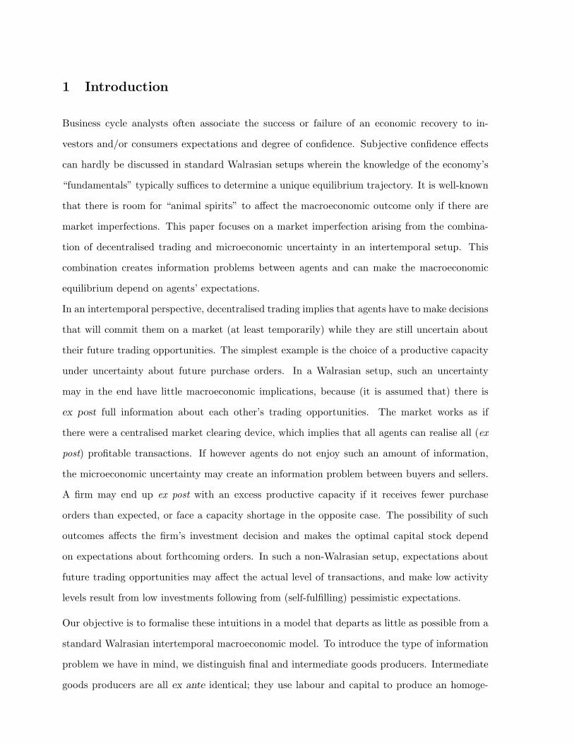
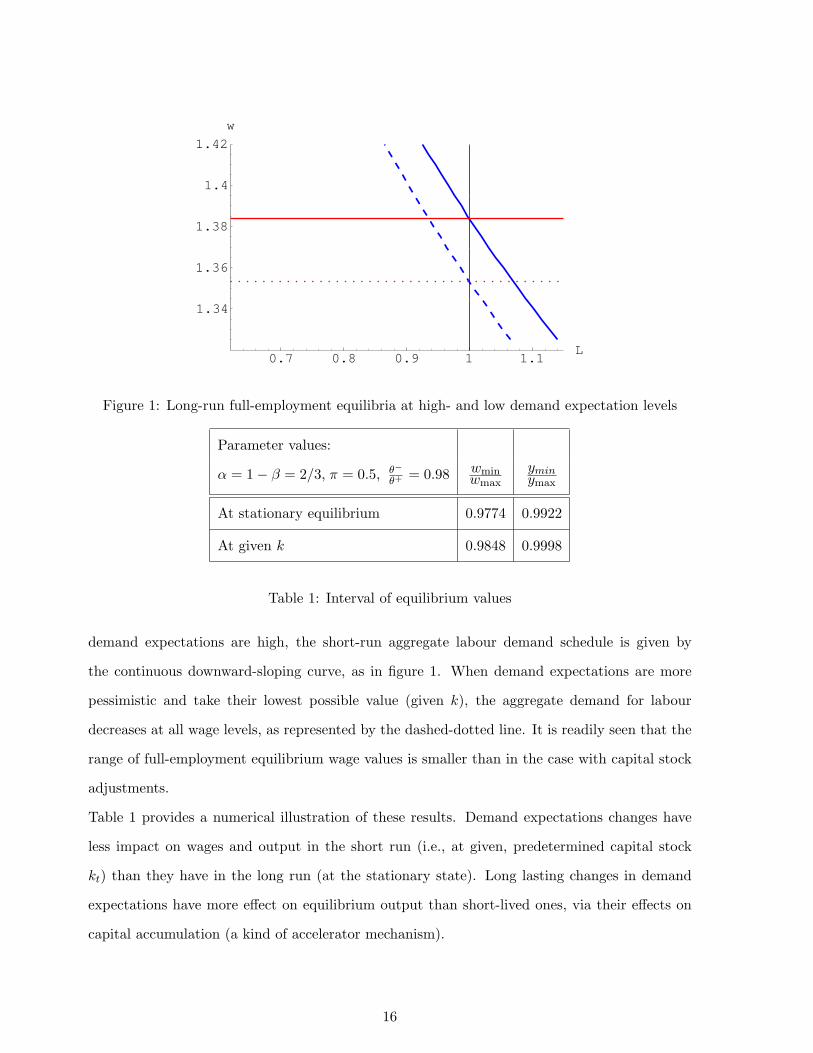
The long run effects of demand expectations on the aggregate labour demand and on full-

employment equilibrium wages are illustrated in figure 1. The figure is drawn under the as-

sumptions of constant returns to scale and π = 0.5, α = 1 − β = 2/3, θ−/θ+ = 0.98 and

θ+ = 1.1. With constant returns to scale, the long-run labour demand schedule is a horizon-

tal line defined by (19); its position depends on the capital usage cost and also in our setup

on demand expectations qd. In the high-expectations case (qd = q+), all firms are producing

at full-capacity as in the standard Walrasian model; the long-run labour demand schedule is

represented by the continuous horizontal line. With a vertical labour supply (normalised to

1), the full-employment high-expectations equilibrium coincides with the stationary Walrasian

equilibrium. When demand expectations are the most pessimistic (qd = q−), the labour demand

schedule shifts downwards, as shown by the horizontal dotted line. The two downward-sloping

curves represent the corresponding short-run labour demand schedules, i.e., they show the effects

of wage changes on the aggregate demand for labour at given capital stock, respectively k+ in

the high expectations case (represented by a continuous line) and k− in the low expectations

case (dashed line). Lower demand expectations imply lower equilibrium wages.

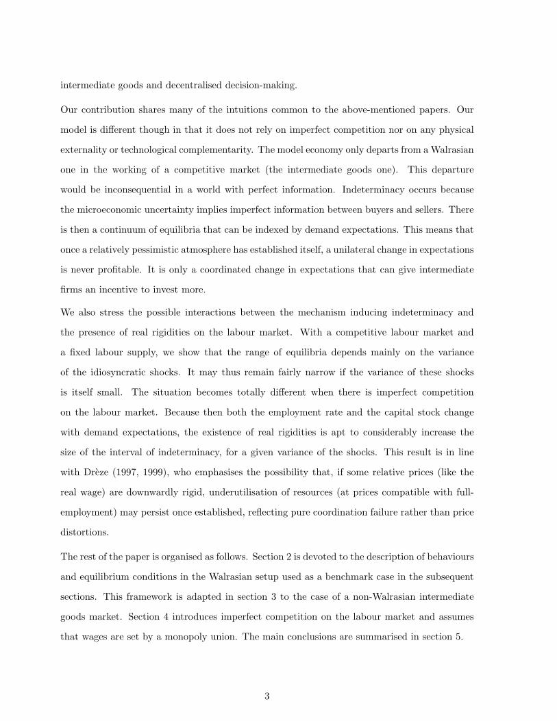
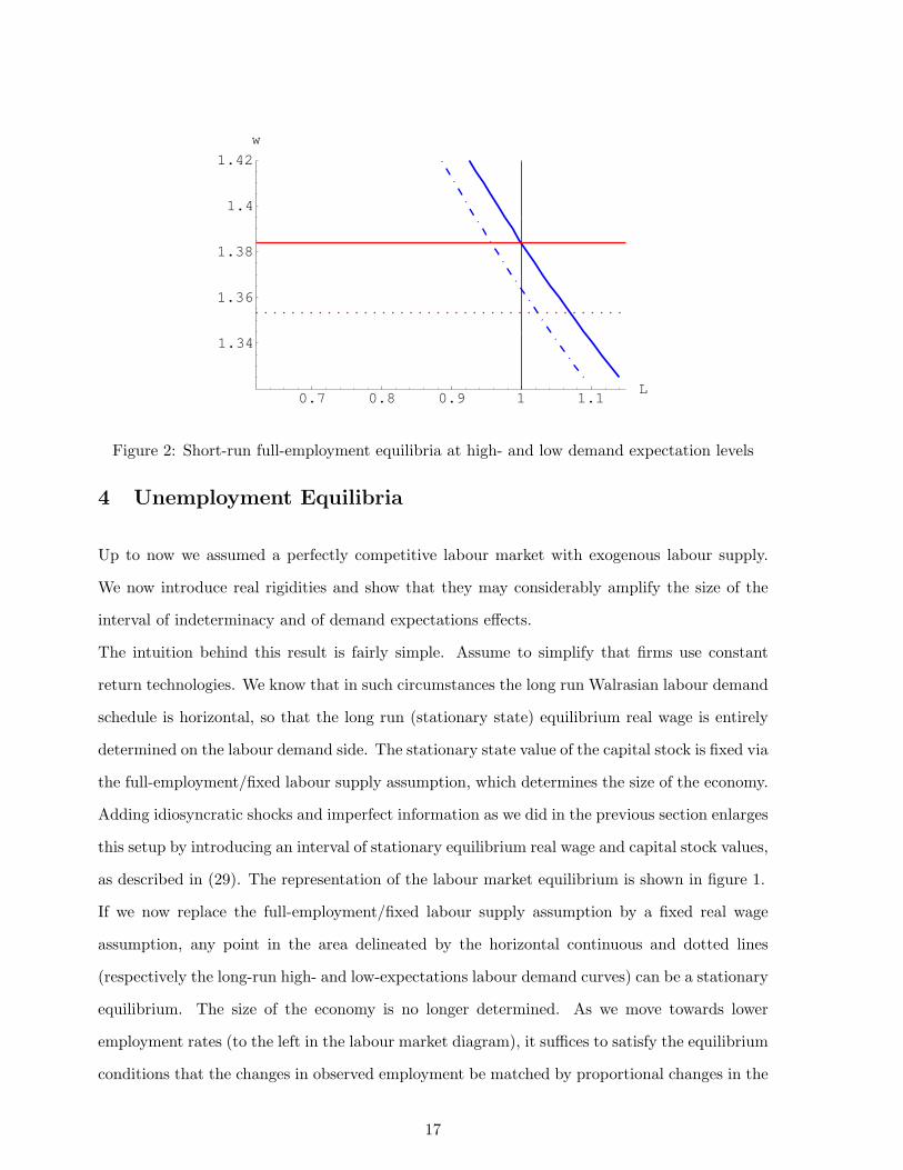
Figure 2 illustrates the effects of demand expectation changes at unchanged capital stock. In

this example, the value of the capital stock is fixed at its Walrasian level (k = k+). When

15

0.7 0.8 0.9 1 1.1L

1.34

1.36

1.38

1.4

1.42

w

Figure 1: Long-run full-employment equilibria at high- and low demand expectation levels

Parameter values:

α = 1− β = 2/3, π = 0.5, θ−θ+ = 0.98 wmin

wmax

yminymax

At stationary equilibrium 0.9774 0.9922

At given k 0.9848 0.9998

Table 1: Interval of equilibrium values

demand expectations are high, the short-run aggregate labour demand schedule is given by

the continuous downward-sloping curve, as in figure 1. When demand expectations are more

pessimistic and take their lowest possible value (given k), the aggregate demand for labour

decreases at all wage levels, as represented by the dashed-dotted line. It is readily seen that the

range of full-employment equilibrium wage values is smaller than in the case with capital stock

adjustments.

Table 1 provides a numerical illustration of these results. Demand expectations changes have

less impact on wages and output in the short run (i.e., at given, predetermined capital stock

kt) than they have in the long run (at the stationary state). Long lasting changes in demand

expectations have more effect on equilibrium output than short-lived ones, via their effects on

capital accumulation (a kind of accelerator mechanism).

16

0.7 0.8 0.9 1 1.1L

1.34

1.36

1.38

1.4

1.42

w

Figure 2: Short-run full-employment equilibria at high- and low demand expectation levels

4 Unemployment Equilibria

Up to now we assumed a perfectly competitive labour market with exogenous labour supply.

We now introduce real rigidities and show that they may considerably amplify the size of the

interval of indeterminacy and of demand expectations effects.

The intuition behind this result is fairly simple. Assume to simplify that firms use constant

return technologies. We know that in such circumstances the long run Walrasian labour demand

schedule is horizontal, so that the long run (stationary state) equilibrium real wage is entirely

determined on the labour demand side. The stationary state value of the capital stock is fixed via

the full-employment/fixed labour supply assumption, which determines the size of the economy.

Adding idiosyncratic shocks and imperfect information as we did in the previous section enlarges

this setup by introducing an interval of stationary equilibrium real wage and capital stock values,

as described in (29). The representation of the labour market equilibrium is shown in figure 1.

If we now replace the full-employment/fixed labour supply assumption by a fixed real wage

assumption, any point in the area delineated by the horizontal continuous and dotted lines

(respectively the long-run high- and low-expectations labour demand curves) can be a stationary

equilibrium. The size of the economy is no longer determined. As we move towards lower

employment rates (to the left in the labour market diagram), it suffices to satisfy the equilibrium

conditions that the changes in observed employment be matched by proportional changes in the

17

capital stock, and that both the employment and the capital stock changes be proportional to

the changes in expected output. For each employment level, demand expectations may of course

be high or low (resp. q+ and q−). The ratio between the high- and low-expectation values of

the variables remains unchanged. The level of the variables is no longer defined, as each of them

(expectations, capital stock and employment level) decreases at the same rate8.

This is obviously a too simple and extreme case. A more general representation should take into

account the wage adjustments induced by unemployment changes. In order to take such wage

adjustments into account, we now consider a simple right-to-manage-monopoly-union model.

We assume that the monopoly union behaves myopically and maximises in each period a static

objective function with the current employment and real wage rates as arguments. This is

admittedly ad hoc, but will suffice to illustrate the effects of real rigidities in the imperfect

information setup examined so far. With perfect information, this representation would yield a

standard equilibrium unemployment (nairu) model, with a unique equilibrium unemployment

rate (see for instance Layard etal. (1991)). This representation thus provides a nice benchmark

case.

Trade Union Behaviour

Let function U(Lt, ωt) represent the preferences of the monopoly union over employment L and

real wage ω in period t. Function U is increasing and quasi-concave in its arguments.

The union chooses the wage of period t given the labour demand schedule at given capital stock

kt. Assuming a Cobb Douglas technology (see appendix 1 for details on the behaviour of firms

in that case), the union’s problem can be represented as follows:

maxωt

U(Lt, ωt) , (30)

subject to Lt = π

(α θ−

ωt

) 11−α

kβ

1−αt + (1− π)

(qdt

θ+

) 1α

k− β

αt . (31)

The optimality condition for wt implies that the wage rate be such that the marginal rate of

substitution between wage and employment is equal to (the absolute value of) the wage elasticity8This case is an example (admittedly a very specific one) of a Walras-Keynes equilibrium as defined in Dreze

(1997).

18

of employment, that is, the optimal wage rate must satisfy:

ωt

Lt

Uω(Lt, ωt)UL(Lt, ωt)

= |ηt| , (32)

where ηt stands for the wage elasticity of aggregate labour demand. It can be shown to be:

|ηt| = 11− α

π`−tLt

<1

1− α, (33)

where π `−tLt

represents the weighted proportion of firms experiencing a low productivity shock.

Because the labour demand of sales-constrained firms is not sensitive to the wage rate, the wage

elasticity of aggregate employment is (in absolute value) smaller than in the perfect information

case. At given capital stock, it is furthermore decreasing in the aggregate employment level

since the weighted proportion of supply-constrained firms then decreases.

By using (25)-(27) in (33), the inverse of |ηt| can be written as:

1|ηt| = (1− α)

ϑ(xt)π

, where 1 ≤ xt ≤ q+t

q−tand ϑ− ≤ ϑ(xt) ≤ ϑ+ . (34)

The inverse of |ηt| thus takes values in the interval:

(1− α)ϑ−

π≤ 1

|ηt| ≤ (1− α)ϑ+

π. (35)

The union’s optimal wage will thus be larger, ceteris paribus, in situations with larger demand

expectations (larger values of xt), because the aggregate labour demand becomes less sensitive

to the wage rate.

Equilibrium Unemployment

Definition

An equilibrium with unemployment in period t is a vector of prices {pt, rt+1, ωt} such that, at

given capital stock kt and given expectations on marginal utility of consumption λt+1, future

demand level qdt+1 and future wage ωt+1, the following conditions are satisfied:

1. final and intermediate goods producers maximise expected profits; consumers maximise

utility;

19

2. on the intermediate goods markets, a proportion π of firms experiences a low productivity

shock and produces q−t , a proportion 1 − π experiences a high productivity shock and

produces qdt ; there is competitive equilibrium on the final good market;

3. on the labour market, the wage rate is set by the union of workers and may imply unem-

ployment.

The equilibrium conditions on the final and intermediate goods market are thus unchanged (see

equations (21) and (22)). On the labour market, the equilibrium condition (23) is replaced by:

L(kt, ωt, qdt ,Θ) = π `(kt, ωt, θ

−) + (1− π) `d(kt, qdt , θ+) ≤ 1 , (36)

where ωt is given by (32).

As in the full-employment case, the equilibrium so defined is not uniquely determined. With

decentralised trading and microeconomic uncertainty (θ− < θ+ and π ∈]0, 1[), the equilibrium

unemployment rate is not uniquely defined and depends on demand expectations9.

Illustration

For illustration purposes, let us use the following specific formulation of the union’s objective

function:

U(Lt, ωt) =

(1 +

1aLb

t

)−1 (1− ω0

ωt

)c

with a > 0, and 0 < b, c ≤ 1 . (37)

The optimal wage rate is then given by:

ωt ={

1 +c

b

1|ηt|

[1 + aLb

t

]}ω0 , (38)

where ω0 can be interpreted as unemployment benefit. In the particular case where c = b and

a → 0, the wage-setting rule is the one of a utilitarian trade-union with logarithmic preferences.

The wage setting-rule would then be a horizontal line in the ω − L space. Our numerical

example is based on the same values as in the previous section for the labour demand function

(π = 0.5, α = 1 − β = 2/3, θ−/θ+ = 0.98, θ+ = 1.10), and on the following parameter values:

a = 0.5, b = 1.0, c = 0.25, ω0 = 1.10 for the union’s objective function. The value of ω0

9This is consistent with the empirical findings of Lubrano et al. (1996) and Shadman-Sneessens (1998),

who find that the equilibrium unemployment rate is not uniquely defined and is affected by both demand- and

supply-side variables.

20

was chosen so as to reproduce the characteristics of the standard Walrasian full-employment

equilibrium in the high-expectations case (qd = q+).

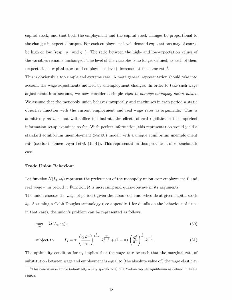
The locus of stationary unemployment equilibria obtained with these formulations and param-

eter values is reproduced in figure 3. The two long-run horizontal schedules are the same ones

as in figure 1. They represent the long run labour demand behaviours (with capital stock

adjustments taken into account) in the two extreme cases with respectively high- and low- de-

mand expectations. The two parallel upward-sloping schedules represent the wage-setting rule

(38) in the same two extreme cases. In the low-expectations case (dashed-dotted line), the

(absolute value of the) wage elasticity |η| is higher, and the optimal wage lower. The intersec-

tion between the two continuous lines determines the high-expectations stationary equilibrium

(with x = qd/q− = q+/q− > 1). By construction it coincides with the Walrasian equilibrium.

The intersection between the dotted horizontal line and the upward-sloping dashed-dotted line

determines the low-expectations stationary equilibrium (with x = qd/q− = 1). In this nu-

merical example, the latter entails an equilibrium unemployment rate of about 20%. The two

downward-sloping schedules represent the short-run (i.e. at given capital stock) labour demand

behaviours. Because the stationary equilibrium value of the capital stock is much lower in

the low-expectations case, the corresponding short-run labour demand schedule (the downward-

sloping dashed-dotted line) is far on the left of its high-expectations counterpart (the continuous

downward-sloping line). All intermediate cases can be similarly obtained, by varying the value

x = qd/q−. The locus of all stationary unemployment equilibria is represented by the thick

dark dashed line of figure 3. Changes in demand expectations generate pro-cyclical real wage

changes, and contra-cyclical changes in “equilibrium unemployment”.

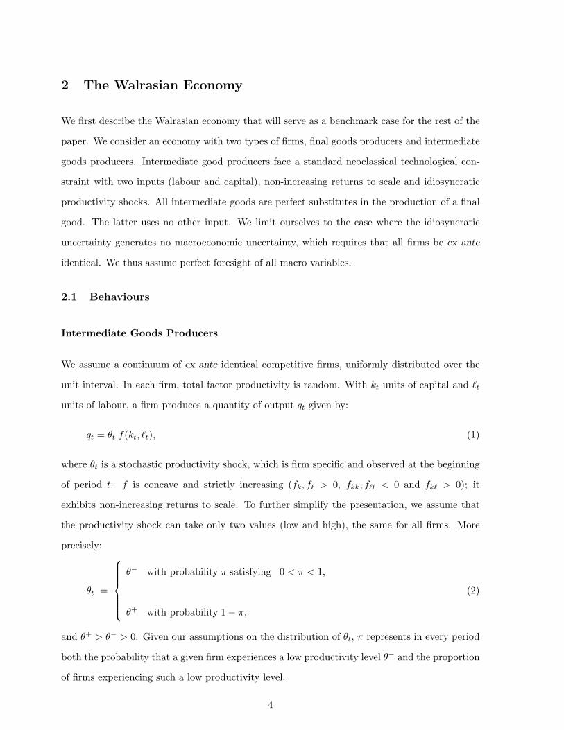
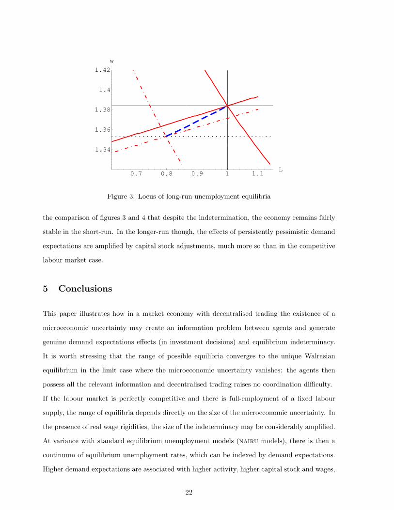
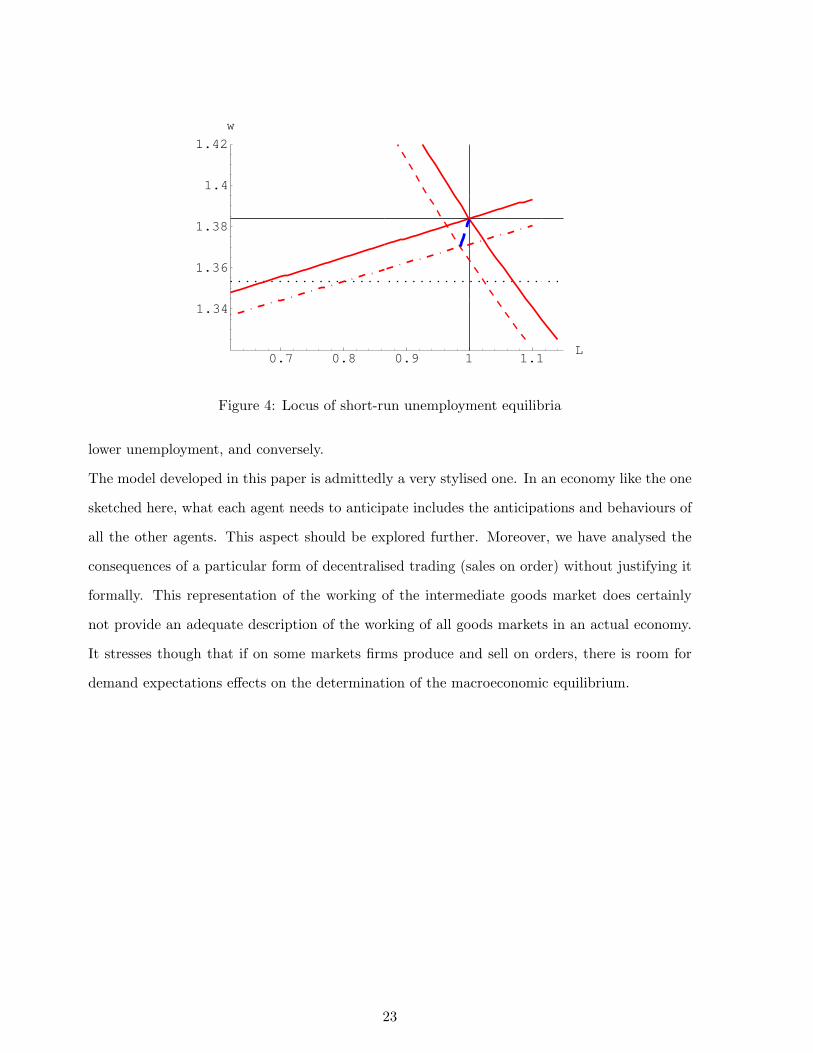
In the short-run, at fixed predetermined capital stock, (unanticipated) changes in demand ex-

pectations cannot have such an enormous impact on equilibrium unemployment. Figure 4 re-

produces the same information as figure 3 for the high-expectations case. The low-expectations

case is now computed at unchanged capital stock. The change in demand expectations shifts the

labour demand schedule to the left, but at unchanged capital stock the shift is limited. The locus

of all short-run unemployment equilibria (when the initial capital stock is at a value compatible

with full-employment) is represented by the thick dark dashed line of figure 4. It is clear from

21

0.7 0.8 0.9 1 1.1L

1.34

1.36

1.38

1.4

1.42

w

Figure 3: Locus of long-run unemployment equilibria

the comparison of figures 3 and 4 that despite the indetermination, the economy remains fairly

stable in the short-run. In the longer-run though, the effects of persistently pessimistic demand

expectations are amplified by capital stock adjustments, much more so than in the competitive

labour market case.

5 Conclusions

This paper illustrates how in a market economy with decentralised trading the existence of a

microeconomic uncertainty may create an information problem between agents and generate

genuine demand expectations effects (in investment decisions) and equilibrium indeterminacy.

It is worth stressing that the range of possible equilibria converges to the unique Walrasian

equilibrium in the limit case where the microeconomic uncertainty vanishes: the agents then

possess all the relevant information and decentralised trading raises no coordination difficulty.

If the labour market is perfectly competitive and there is full-employment of a fixed labour

supply, the range of equilibria depends directly on the size of the microeconomic uncertainty. In

the presence of real wage rigidities, the size of the indeterminacy may be considerably amplified.

At variance with standard equilibrium unemployment models (nairu models), there is then a

continuum of equilibrium unemployment rates, which can be indexed by demand expectations.

Higher demand expectations are associated with higher activity, higher capital stock and wages,

22

0.7 0.8 0.9 1 1.1L

1.34

1.36

1.38

1.4

1.42

w

Figure 4: Locus of short-run unemployment equilibria

lower unemployment, and conversely.

The model developed in this paper is admittedly a very stylised one. In an economy like the one

sketched here, what each agent needs to anticipate includes the anticipations and behaviours of

all the other agents. This aspect should be explored further. Moreover, we have analysed the

consequences of a particular form of decentralised trading (sales on order) without justifying it

formally. This representation of the working of the intermediate goods market does certainly

not provide an adequate description of the working of all goods markets in an actual economy.

It stresses though that if on some markets firms produce and sell on orders, there is room for

demand expectations effects on the determination of the macroeconomic equilibrium.

23

References

Benhabib J. and R.E.A. Farmer (2000), 3indeterminacy and Sunspots in Macroeconomics”,

in J.B.Taylor and M.Woodford, Handbook of Macroeconomics, Vol. I A, Amsterdam: North-

Holland

Blanchard-Kiyotaki (1987) “Monopolistic Competition and the Effects of Aggregate Demand”

American Economic Review 77(4), 647-666.

Bryant (1983) “A Simple Rational-Expectations Keynes-Type Model”, Quartely Journal of Eco-

nomics, 98, 525-528.

Cooper and John (1988) “Coordinating Coordination Failures in Keynesian Models”, Quartely

Journal of Economics, 103, 441-463.

Diamond (1982) “Aggregate-Demand Management in Search Equilibrium”, Journal of Political

Economy,90-5, 881-894.

Dreze J.H. (1997), “Walras-Keynes Equilibria, Coordination and Macroeconomics”, European

Economic Review, 41:9, 1737-1762.

Dreze J.H. (1999)“On the Macroeconomics of Uncertainty and Incomplete Markets”, Presiden-

tial Address, 12th World Congress of the International Economic Association, CORE DP 9964,

Universite catholique de Louvain, Louvain-la-Neuve.

Gali (1996) “Multiple Equilibria in a growth Model with Monopolistic Competition”, Economic

Theory, 8, 251-266.

Hart O. (1982) “ A Model of Imperfect Competition with Keynesian Features”, Quartely Journal

of Economics, 97, 109-138.

Heller W. (1986) “Coordination Failure under Complete Markets with Applications to Effective

Demand”, in W.P.Heller, R.M.Starr and D.A.Starrett, eds, Equilibrium Analysis: Essays in

Honor of Kenneth J. Arrow,, vol 2, Cambridge: Cambridge University Press.

Howitt P. and R.P. McAfee (1992) “Animal Spirits”, American Economic Review82(3), 493-507.

Jones, L.E. and R.E. Manuelli (1992), “The Coordination Problem and Equilibrium Theories of

Recessions” American Economic Review, Vol. 82(3), 451-471.

Kiyotaki(1988) “Multiple Expectational Equilibria under Monopolistic Competition”, Quartely

Journal of Economics 103(4), 695-713.

24

Layard, R., S. Nickell and R. Jackman (1991), Unemployment, Macroeconomic Performance

and the Labour Market. Oxford: Oxford University Press.

Lubrano, M., F. Shadman-Mehta and H.R. Sneessens (1996),“Real Wages, Quantity Constraints

and Equilibrium Unemployment: Belgium, 1955- 198”, Empirical Economics, 21, 427-457.

Roberts, J. (1987), “An Equilibrium Model with Involuntary Unemployment at Flexible, Com-

petitive Prices and Wages”, American Economic Review, Vol. 77(5), 856-874.

Roberts, J. (1989), “Involuntary Unemployment and Imperfect Competition: A Game-theoretic

Macromodel ”, in G.Feiwel, ed., The Economics of Imperfect Competition and Employment:

Joan Robinson and Beyond, London: MacMillan.

Shadman-Mehta, F., and H.R. Sneessens (1998), “Demand-Supply Interactions and Unemploy-

ment Dynamics : Can there be Path Dependency? The case of Belgium, 1955-1994”, IRES

DP9817, Department of Economics, Universite catholique de Louvain, Louvain-la-Neuve.

Silvestre J. (1995) “Market Power in Macroeconomic Models: New Developments”, Annales

d’economie et de statistique, 37/38, 319-356.

25

Appendix 1: Firms’ behaviour with Cobb Douglas technologies

Assume the following Cobb Douglas technology

qt = θt `αt kβ

t , α + β ≤ 1 , (39)

The Walrasian economy

The employment and production decisions are

`±t = `(kt, ωt, θ±) =

[α θ±

ωtkβ

t

] 11−α

and q±t = q(kt, ωt, θ±) = θ±

[α θ±

ωtk

β/αt

] α1−α

(40)

Π−t (resp. Π+t ) then becomes

Π±t = (1− α) pt q(kt, ωt, θ±) (41)

The optimality conditions on kt+1 writes as follows

rt+1 + δ

pt+1= β

π θ−

(α θ−

ωt+1

) α1−α

+ (1− π) θ+

(α θ+

ωt+1

) α1−α

(kt+1)

− 1−α−β1−α , ∀ t. (42)

Therefore,

kt+1 =[

β

νt+1

] 1−α1−α−β

π θ−

(α θ−

ωt+1

) α1−α

+ (1− π) θ+

(α θ+

ωt+1

) α1−α

1−α1−α−β

, ∀ t. (43)

By using the optimality condition (43), one checks easily that the expected value of profits is

given by:

(1− α− β) pt

[ (α

ωt

)α (β

νt

)β [E(θ)

11−α

]1−α] 1

1−α−β

≥ 0, ∀ t.

Expected profits are nil in the constant returns-to-scale case, positive otherwise.

The non-Walrasian economy

`dt = `d(kt, q

dt , θ+) =

[qdt

θ+

]1/α

(kt)−β/α ≤ `+

t . (44)

In t, a firm installs a capital stock level kt+1 given by the following first-order optimality condi-

tion:

νt+1 =β

αωt+1

π

(α θ−

ωt+1

)1/1−α

(kt+1)α+β−1

1−α + (1− π)

(qdt+1

θ+

)1/α

(kt+1)−α+β

α

. (45)

26

Appendix 2: Stationary equilibria with full employment

The general case

In a stationary equilibrium of the Walrasian economy, the investment equation (6) and the

labour market clearing condition (14) become

ρ + δ = π πk(k, ω, θ−) + (1− π) πk(k, ω, θ+) (46)

1 = π `(k, ω, θ−) + (1− π) `(k, ω, θ+) (47)

and determine the stationary values (k∗, ω∗).

In a stationary equilibrium of the non-Walrasian economy, the investment equation (19) and the

labour market clearing condition (23) become

ρ + δ = π πk(k, ω, θ−) + (1− π) πdk(k, qd, ω, θ+) (48)

1 = π `(k, ω, θ−) + (1− π) `d(k, qd, θ+) (49)

and determine the stationary values (k, ω) in function of qd.

Let ω− and k− (resp. ω+ and k+) represent the real wage and capital stock level in a stationary

equilibrium where firms have persistently low (resp. high) demand expectations, i.e. where

qd = q− (resp. qd = q+).

Substituting qd by q− and q+ respectively into (48-49) makes obvious that k− < k+ and ω− <

ω+.

Furthermore, when qd = q+ = q(k, ω, θ+), (49) is obviously identical to (47) because

`d(k, qd = q+, θ+) = `(k, ω, θ+) = `+.

Similarly, (48) is identical to (46) when qd = q+: indeed,

πdk(k, qd, θ+)

∣∣∣qd=q+

= −ωd `d(k, qd, θ+)

d k

∣∣∣∣∣qd=q+

= −ωfk(k, `d)f`(k, `d)

∣∣∣∣∣`d=`+

= θ+ fk(k, `+) since ω = θ+ f`(k, `+)

= πk(k, ω, θ+).

27

Consequently, (48-49) is identical to (46-47) when qd = q+ and thus admits the same solution:

i.e., (k+, ω+) = (k∗, ω∗).

The Cobb Douglas case

Let us first focus on the stationary state equilibrium of the Walrasian economy. The labour

market clearing condition (14) gives the following relationship between the equilibrium real

wage and the installed capital stock

ωt = α θ− kβt

π + (1− π)

(θ+

θ−

)1/(1−α)

1−α

(50)

From (43), one has

k∗ =(

β

ν

ω∗

α

) 1−α1−α−β

(α θ−

ω∗

) 11−α−β

π + (1− π)

(θ±

θ−

)1/(1−α)

1−α1−α−β

. (51)

Substituting ω∗ by its value from (50) into the demand for capital (51) gives the following

stationary capital stock level:

k∗ =(

β

ν

) 11−β

π + (1− π)

(θ+

θ−

)1/(1−α)

1−α1−β

. (52)

In a stationary equilibrium of the non-Walrasian economy, (14) implies that when firms have

persistently low (resp. high) demand expectations one has

w± = α θ− (k±)β

π + (1− π)

(θ±

θ+

)1/α (θ±

θ−

)1/(1−α)

1−α

. (53)

Similarly from (45),

k± =

(β

ν

ω±

α

) 1−α1−α−β

(α θ−

ω±

) 11−α−β

π + (1− π)

(θ±

θ+

)1/α (θ±

θ−

)1/(1−α)

1−α1−α−β

. (54)

Introducing (53) into the capital labour demand (54) then gives

k± =(

β

ν

) 11−β

π + (1− π)

(θ±

θ+

)1/α (θ±

θ−

)1/(1−α)

1−α1−β

. (55)

A comparison between (52) and (55) makes obvious that k− < k+ = k∗. Furthermore, dividing

(54) for k+ by (54) for k− gives the value of the ratio k+/k− given in the main text. After

introducing (55) into (53), one obtains easily the same value for the ratio w+/w−.

28