Legal Reform and Loan Repayment:

The Microeconomic Impact of Debt Recovery Tribunals

in India∗

Sujata Visaria†

Boston University

April 2006

∗I am grateful to Charles Calomiris, Rajeev Dehejia, Rohini Pande and Miguel Urquiola for theirguidance and encouragement. Many thanks to Maharukh Dastur, Krishnava Dutt, Nachiket Mor,Sekar, V. R. Sahasrabuddhe, Bhavna Sharma and several others at the bank where I collected thedata, and M.A. Batki, N.V. Deshpande and G.S. Hegde at the Reserve Bank of India. This paper hasbenefitted from discussions with Francesco Brindisi, Rajeev Cherukupalli, Dilip Mookherjee, LenaEdlund, Ivan Fernandez-Val, Ray Fisman, Indradeep Ghosh, Tanu Ghosh, Wojciech Kopczuk, PrithaMitra, Anirban Mukhopadhyay, Francisco Perez-Gonzalez, Kiki Pop-Eleches, Sanjay Reddy, EricVerhoogen and Till von Wachter. Thanks to seminar participants at Boston University, ColumbiaUniversity, Hong Kong University of Science & Technology, University of Maryland, University ofToronto, the SSRC Fellows 2004 conference, NEUDC 2004 and BREAD Fall 2005 conferences. Thisresearch was supported by the Center for International Business Education at Columbia University,the Social Science Research Council’s Program in Applied Economics with funds provided by theJohn D. and Catherine T. Macarthur Foundation, and the Institute for Financial Management andResearch. Thanks also to the Graduate Fellows program at the Institute for Social and EconomicResearch and Policy at Columbia University. The usual disclaimers apply.

†Department of Economics, Boston University, 270 Bay State Road, Boston, MA 02215. E-mail:svisaria@bu.edu

Abstract

This paper investigates the micro-level link between judicial quality and eco-nomic outcomes. It uses a loan-level data set from a large Indian bank to es-timate the impact of a new quasi-legal institution, Debt Recovery Tribunals,which are aimed at accelerating banks’ recovery of non-performing loans. I usea differences-in-differences strategy based on two sources of variation: the mon-etary threshold for claims to be eligible for these tribunals, and the staggeredintroduction of tribunals across Indian states. I find that the establishment oftribunals reduces delinquency in loan repayment by between 3 and 11 percent.The effect is statistically significant within loans as well: for the same loan, in-stallments that become due after the loan becomes treated are more likely to bepaid up on time than those that become due before. Furthermore, interest rateson loans sanctioned after the reform are lower by 1.4-2 percentage points. Theseresults suggest that legal reform and the improved enforcement of loan contractscan reduce borrower delinquency, and can lead banks to provide cheaper credit.Thus the paper illustrates a microeconomic mechanism through which improve-ments in legal institutions might affect credit market outcomes.

1 Introduction

It is common in India for people to age considerably while they wait for the courts

to resolve their legal disputes. The notorious Bofors gun scandal is an illustration.

The scandal broke in 1987 but is far from resolved even today. In the meanwhile, two

of the key accused: India’s defense secretary at the time of the deal, and the Indian

agent of the Bofors company, have died (of natural causes). Former prime minister

Rajiv Gandhi was chargesheeted in 1997; six years after he had been assassinated.

His name was cleared seven years later, in 2004. While the Bofors case is complex

and high-profile, it is indicative of a widespread phenomenon: in the Indian system

most types of legal suits take very long to resolve. In fact, the quality of formal

judicial institutions is poor in many developing countries, transition economies, and

even some developed countries. Cases in court are regularly subject to long delays,

judges and court officials are corrupt, or the courts are captured by the elite.

In this paper I try to examine what effect this has on market outcomes. Previous

studies have found that across countries, an index of judicial quality can predict en-

trepreneurial investment and economic growth. However, a specific policy measure in

India allows me to examine a particular micro-level mechanism at work. In 1993, the

Indian government passed a national act allowing the establishment of Debt Recovery

Tribunals (DRTs) across India. These tribunals are a new quasi-legal institution set

up to process legal suits filed by banks against defaulting borrowers. They follow a

streamlined legal procedure that emphasizes speedy adjudication of cases and swift

execution of the verdict.

Two aspects of this reform allow the identification of its effects. One, the mone-

tary threshold for claims to be filed in a DRT is Rupees 1 million (approximately US$

20,000). Two, there is variation in the timing of tribunal establishment in different

states. Neither the monetary threshold nor the timing of DRT placement appears

to be correlated with other factors which may influence the ability or willingness of

borrowers to repay their loans. My data consist of loan level records collected from

a large private sector bank with a national presence. They contain detailed informa-

tion about the contractual terms of the loans, their repayment schedule and actual

1

repayment in each quarter when an installment becomes due. Loans that are late on

repayment of more than Rupees 1 million at the time of the legal reform are poten-

tially treated by DRTs. Therefore I compare the change in the repayment behavior

of these loans after DRTs are established, to the change in the repayment behavior

of other loans (those with less than Rupees 1 million overdue). For loans with more

than Rupees 1 million overdue, the establishment of a tribunal increases the likelihood

that an installment is paid on time. Furthermore, this effect holds within loans as

well: for the same loan, installments that become due after a tribunal is established

are more likely to be paid up on time than installments that become due before.

Several robustness checks reinforce these findings: the effects remain significant even

after controlling for state-level time-varying unobservable factors (by including state

× quarter fixed effects), and allowing different time-varying unobservables for loans

above and below the Rupees 1 million threshold.

As evidence of the economic impact of this reform, I find further that the estab-

lishment of a DRT leads to a change in the contractual terms of new loans given out

subsequently. While the size of an average loan does not change significantly, the

interest rate on new loans tends to be lower than that on comparable older loans by

1 to 2 percentage points. This suggests that improved repayment behavior lowers the

risk of default and allows the bank to provide cheaper credit.

The rest of the paper is organized as follows. Section 2 situates the paper within

the existing literature. Section 3 discusses the background against which the DRT

Act was introduced. Section 4 describes in detail the institution of DRTs: their main

features, and the manner in which the DRT act was implemented. It also provides

some suggestive evidence on the effectiveness of DRTs. Section 5 presents a simple

theoretical framework to explain the phenomenon studied here. Section 6 describes

the data, section 7 presents the empirical strategy, and sections 8 and 9 present the

empirical results. Section 10 concludes the paper.

2 Literature

Recent empirical work has shown that institutional quality is an important determi-

nant of economic development (Acemoglu et al. 2001, Banerjee & Iyer 2003). For

2

example, legal systems that protect shareholders and creditors lead to lower concen-

trations of share-holding (La Porta et al. 1998). The enforcement of these rules is

important as well. Demirguc-Kunt & Maksimovic (1998) find that in countries with

efficient judiciaries, firms are more likely to get external funds for long-term invest-

ment. Further, the nature of the rules can affect the quality of their implementation:

procedural formalism can make judicial processes cumbersome, and entrepreneurs

perceive systems with simpler, less bureaucratic procedures as providing better ser-

vice (Djankov et al. 2003). This paper is also concerned with the procedural aspect

of judicial quality. It focuses on one dimension of judicial quality, viz. the time taken

to resolve (debt recovery) suits, and examines how this affects behavior of borrowers

and lenders in the credit market. A recent policy reform in India provides a setting to

identify these effects relatively cleanly. The paper thus illustrates a micro-economic

mechanism through which the quality of the judiciary can affect economic outcomes.

3 Background

The Indian court system is notorious for the time taken to resolve cases. In his

case study of two district courts in northern India, Moog (1997) remarks that the

most effective method of dispute resolution in these courts may well be the out-of-

court settlements, withdrawals and compromises by litigants attempting to avoid the

inefficiencies in processing legal suits. Cases in both district and high courts are

subject to long delays. In 1985, the high courts had roughly 570,000 original civil

suits pending, of which 36 percent had been pending longer than three years. The

situation was disproportionately bad for civil cases of asset liquidation: 40 percent

had been pending longer than eight years (Law Commission of India 1988).1

While legal scholars point to various reasons for the inefficiency of the court sys-

tem, it is widely acknowledged that procedural loopholes are an important factor.

Civil courts follow the Code of Civil Procedure (1908). This code allows for numer-

ous applications, counter-applications and “special leaves” by both the plaintiff and1Note that the life of a civil suit is likely to be even longer, since there are multiple appeals

possible. Even after a final judgment is arrived at and all appeals are exhausted, the execution ofthe verdict can also be contested, and that ruling can be appealed as well.

3

the defendant. Evidence must be presented orally, and hearings tend to be long.2

Judges have wide latitude in determining whether hearings should be adjourned or

new claims added to the plaint (Kohling 2002). Although both central and state

legislatures have attempted to reform the Code by enacting amendments to it, the

general consensus is that these attempts have been unsuccessful.

Judicial inefficiency could affect various sectors of the economy; in this paper

we focus on the effect on the market for corporate bank debt. To understand the

motivation for Debt Recovery Tribunals, I provide below a brief background on non-

performing loans in the Indian banking system.

3.1 Non-performing Loans

In newly independent India, policy-makers set an agenda for the banking sector: it

was to extend credit to various sectors of the economy and promote economic devel-

opment. This objective overrode concerns about the financial health of banks. Poorly

performing public sector banks could expect to be recapitalized by the government.

Private sector banks were also heavily regulated.3

This led to a high volume of non-performing loans in the banking system. In

1996, 18.1 percent of the gross loans of public sector banks were non-performing.

Private sector banks, which have only about 20-25 percent of the assets in the bank-

ing sector, reported 10 percent of their gross loans as non-performing. When India

began the liberalization of its financial sector in the early 1990s, the Narasimham

Committee on the Financial System (Government of India 1991) argued that unless

proactive measures were taken, these bad loans could jeopardize the entire financial

system. The Reserve Bank of India responded with several measures. In 1992, it

provided an objective classification system for banks’ assets. Whereas earlier banks

could use a subjective Health Code system, now a loan would be classified as non-

performing if payment of interest or repayment of installment of principal or both2Law Commission of India (1988) provides a vivid account. Four judges of the Supreme Court

spent all of 1981 hearing oral arguments in two cases. Arguments in the first case began on December9, 1980 and continued until April 30, 1981. The court was closed for summer recess from the firstweek of May to the third week of July. The second case was heard from August 4 until November16. For the rest of 1981 the judges prepared their judgments.

3All commercial banks were required to make 40 percent of their loans to the “priority sector”:agriculture and allied activities, small scale industries and minority communities.

4

had remained unpaid for a certain pre-specified period or more.4 It also imposed

stricter accounting standards and greater reporting requirements and required that

banks hold in reserve larger proportions of the value of outstanding loans to cover

themselves against possible default.

These changes created incentives for banks to reduce the volume of their non-

performing loans. Whereas in the short term, banks can achieve this by restructuring

the loan or writing off the unrecoverable part, a true improvement in the bank’s

balance sheet requires that money be recovered from the defaulting borrower. Since

most bank loans in India are secured by collateral, this requires that the collateral

be liquidated.5

3.2 Debt Recovery and Judicial Quality

To recover a non-performing loan, secured or not, a bank must first obtain a court

order. Before 1994, this involved filing a legal suit in the civil court system. In

this suit, the bank must state the particulars of the case, and request that the court

direct the borrower to pay the money to the bank (the directive is termed a money

decree). If the loan is unsecured the bank must request that the court liquidate the

firm’s assets (“wind up” the firm) and distribute the proceeds from liquidation among

all creditors according to the priority of their claim. If the loan is secured, it must

request that the court enforce its security interest, i.e. allow the sale of collateral so

that the bank may recover its dues.

In this setting, the benefit from filing a legal suit against a defaulting borrower has

been low, and the cost has been high. The bankruptcy procedure for firms has also

been time-consuming, and bankers complain that it creates incentives for borrowers

to mismanage funds.4This pre-specified period was fixed at four quarters for the financial year ending on March 31,

1993. It was to be decreased to three quarters in 1994 and to two quarters (180 days) in 1995 andthereafter (Reserve Bank of India 1999; 2003). A further notification since then has decreased it toone quarter (90 days) beginning 2004.

5Pistor & Wellons (1999) report that 90 percent of bank loans in India are secured.

5

4 Debt Recovery Tribunals

In 1981 the Tiwari Committee investigated the legal difficulties faced by banks and

recommended the establishment of special tribunals for the recovery of debt. It

suggested that these tribunals use a simple procedure guided only by the principles

of natural justice. The Narasimham Committee endorsed this proposal in 1991,

leading the Government of India to pass a new act in 1993, known as the “Recovery

of Debts due to Banks and Financial Institutions Act” (DRT Act).

4.1 The DRT Act

The act came into force on June 24th, 1993.6 It allows the Government of India to

establish debt recovery tribunals (DRTs) “for expeditious adjudication and recovery

of debts due to banks and financial institutions”, and to specify their territorial

jurisdiction.

A debt recovery suit against a borrower can be filed in a DRT only if the claim is

larger than Rupees 1 million (approximately $20,000). The rationale for this stipu-

lation appears to have been as follows. First, by restricting the size of the claim that

would be eligible for DRTs, this avoids overcrowding the DRTs. Second, given the

large fixed cost of litigation, the larger non-performing loans are also most attractive

to recover. The DRTs were envisioned as helping banks recover bad loans from the

larger corporate borrowers. The exact threshold appears to have been chosen because

it was a convenient round number. There is no evidence to suggest that there were

any economic reasons for this choice.7

Debt Recovery Tribunals are a quasi-legal institution dealing exclusively with

debt recovery cases: cases where the bank or financial institution claims money is to

be recovered from a borrower. They are “quasi-legal” in that they are established by

the executive arm of the government and fall under the purview of the Ministry of

Finance, unlike civil and criminal courts which are part of the judiciary. However,6The records of parliamentary proceedings from the period show that the bill was introduced

into the lower house of parliament (Lok Sabha) on May 13, 1993. It appears to have met with noopposition in parliament, and was passed on August 10, 1993. It came into effect retrospectively.

7An amendment bill is currently pending in the Lok Sabha to reduce the monetary threshold toRupees 500 thousand.

6

the substantive laws governing debt recovery cases remain the same as they were

before. Also, the judge in a DRT (called the presiding officer) must be qualified to

be a district judge in the judicial system, and the same lawyers who are qualified to

appear in civil courts are also qualified to argue in DRTs.

As the act envisions it, the main distinction between DRTs and civil courts is that

DRTs follow a streamlined “summary” procedure. This procedure demands faster

processing and greater accountability by the litigants. The defendant has only thirty

days to respond to summons; he must present a written defense at or before the

first hearing and counter-claims against the bank must be made at the first hearing.8

The act also gives tribunals more power than civil courts had. DRTs are allowed

to make interim orders before the final judgement, so as to prevent defendants from

transferring or disposing of the assets in question. It also provides for swift execution

of the verdict. The “recovery officer” has the authority to attach and sell the property

of the defendant, arrange for a “receiver” to manage the property of the defendant, or

arrest the recalcitrant defendant and detain him in prison. Consistent with the civil

court system the DRT act allows for appeals against a judgement: either party can

appeal against a DRT’s ruling in the Debt Recovery Appellate Tribunal (DRAT).

However the defendant must deposit 75 percent of the awarded amount with the

DRAT before the hearing can take place. The deposit is returned to him if the

DRAT rules in his favor.

4.2 Response to the Debt Recovery Tribunals

Although welcomed by bankers as well as economists, the act also met with opposi-

tion. DRTs had begun to be established in 1994. Soon after Delhi received a DRT

in July 1994, the Delhi Bar Association filed a suit in the Delhi High Court, chal-

lenging the DRT Act as unconstitutional.9 In August 1994 the Delhi High Court8The original DRT Act 1993 did not allow counter-claims. These were introduced in the 2000

Amendment, described in detail in the next sub-section.9They made their case on the following grounds: (i) since the presiding officers of DRTs were

appointed by the Ministry of Finance, the act violated the Directive Principle of State Policy thatthe executive and judiciary be independent; (ii) the act was discriminatory because it did not allowborrowers to make counter-claims against banks; (iii) there was no rationale for making suits admis-sible on the basis of their pecuniary claim; and (iv) the Constitution did not allow the legislature toestablish tribunals for the purpose of debt recovery.

7

stated that it was of the prima facie view that the act may not be valid, and required

the Delhi DRT to stay its operations pending the final verdict. In its final verdict

delivered on March 10th 1995, it accepted the Delhi Bar Association’s argument that

the act was unconstitutional because it violated the independence of the judiciary

from the executive. It also ruled that the act had other flaws: the lack of provisions

for counter-claims and transfer of cases from one DRT to another.10

The central government moved the Supreme Court against this judgement in a

special leave petition.11 On March 18th 1996 the Supreme Court issued an interim

order that notwithstanding any stay order passed in any writ petitions, DRTs should

resume functions. It also asked the central government to amend the act to address

certain legal anomalies. The DRT Amendment Act in 2000 not only increased the

legitimacy of DRTs in the eyes of the judiciary, but also clarified certain procedures.12

The Supreme Court delivered its final ruling on this issue on March 14th 2002. It

stated that the DRT Act was constitutional, and the act as it stood amended was

to be allowed. At this time all pending cases about the constitutional validity of the

act were dismissed.

4.3 Pattern of DRT Establishment

The opposition to the DRT Act led to a particular pattern of establishment of DRTs

which is useful for the empirical strategy. Note first that the DRT Act is a national law

and applies to all states of India, with the sole exception of Jammu & Kashmir. Thus,

at least in theory, states cannot choose whether or not to establish these tribunals.

Second, the authority to establish the tribunals lies with the national government,

which can choose when to give a particular state access to a DRT. (Later in the paper10On the other hand, it stated that the legislature did have the authority to pass this act. However

it took exception to another aspect: whereas before the DRT was established all claims betweenRupees 100,000 and 50,000 had been in the jurisdiction of the Delhi High Court, the act gave DRTsjurisdiction over higher valued claims, viz. Rupees 1 million and above. And yet the judge of a DRTwas only required to have the qualifications of a district court judge. Thus DRTs had been placedon a higher pedestal than high courts, which was considered unacceptable.

11Separate from this, both the Guwahati and Karnataka High Courts ruled against the act, in1999 and 2001 respectively. However according to Article 141 of the Constitution an order of theSupreme Court is binding on all courts of the country and hence these rulings could not have beenimplemented.

12Inter alia, to maintain the independence of the judiciary from the executive, it required that theChief Justice of India be the ex-officio Chair of the selection committee for presiding officers.

8

I discuss in detail the concern that state-level factors may have influenced the timing

of DRT establishment.)

As mentioned before, the central government began establishing DRTs in 1994.

Its objective appears to have been to provide access to tribunals in as much territory

as quickly as possible. Five tribunals were set up in quick succession beginning

in April 1994. Appendix A.1 lists the dates of establishment of DRTs. In many

cases, access was maximized by requiring neighboring states to share the services of a

single tribunal.13 However the ruling of the Delhi High Court brought this process of

establishment to a halt, and no new DRTs were established in 1995. It was only after

the interim order of the Supreme Court in 1996 that DRTs began to be established

again. All the remaining states received DRTs after this, and by 1999 all states of

India had access to a Debt Recovery Tribunal.14

4.4 Performance of DRTs

By March 31st 2003, DRTs had disposed claims worth Rupees 314 billion (amount-

ing to roughly 4 percent of total bank credit to the commercial sector in 2002-03)

and recovered Rupees 79 billion (Government of India 2003). As a first step I ask

whether DRTs were truly more effective at processing debt recovery cases than civil

courts. In the absence of any official information on case processing times, I collected

information on a small random sample of debt recovery cases. These cases were filed

by the same bank whose loan-level data will be used later to estimate the impact of

DRTs. I collected detailed information on the date when the case was filed, the venue

it was first filed in (civil court or DRT), the various stages through which the case

had passed, and the dates on which each case-related event had taken place. Due to

logistical considerations, I could only collect data on cases filed in the Maharashtra

jurisdiction, hence all cases were filed in the Bombay high court or the Mumbai or

Pune DRTs. This does not allow me to separate a secular trend towards lower case13In the empirical work, I classify the states into clusters: groups of states which shared a DRT.14Following that, new DRTs continued to be established and earlier jurisdictions sub-divided among

the new and the old, thus reducing the number of cases each DRT would handle. In the empiricalstrategy, however, I exploit the fact that at any point in time, a loan always faces only one DRT.Therefore I define treatment as a binary variable which switched from 0 to 1 when a loan went fromno exposure to DRTs to exposure to a DRT.

9

processing times across the judiciary, from reductions in case processing times that

are DRT-specific; this caveat must be borne in mind. Note however, that DRTs can

only process claims worth Rupees 1 million or above, whereas civil courts had no

such monetary restriction. This feature will be exploited in the empirical strategy.

It is interesting that the DRTs do not out-perform the Bombay high court on all

dimensions, although on several important ones they do.

Before discussing the summary statistics in Table 1, I describe briefly the various

steps through which a case could pass. A case is filed in a court or DRT by submitting

an original application or a plaint. This states the particulars of the case, and a

request to the court/tribunal for remedial action. The bank can also file an urgent

application, and request “interim relief”, which is usually an injunction preventing

the borrower from disposing off its assets while the matter is sub-judice. In the

Bombay high court there was also the practice of appointing a court receiver, who

could seize the defendant’s assets. Once the application has been filed, the court

issues summons to the defendant, specifying a date when he/she should appear in

court. The defendant appears in court, and replies to the summons by presenting

his side of the case and/or filing a counter-claim against the borrower. At each such

appearance, the court sets a date for the next hearing. Either party may not appear

on this date, in which case the hearing is postponed; it is possible that several dates

are set before a hearing actually takes place. Over the course of these hearings, both

applicant and defendant submit evidence and make oral arguments before the judge

or presiding officer. At any point, the process could end: the borrower could agree

to consent terms, or settle with the bank.15 Alternately, the borrower could file an

application with the Board of Industrial and Financial Reconstruction (BIFR) or its

appellate authority, the AAIFR. This effectively freezes the case in court, until the15If he agrees to consent terms, the court issues a consent decree, and the terms are be executed

privately. If either party reneges on this decree, the aggrieved party can approach the court again.Settlements occur “out of court”.

10

BIFR makes a decision.16

After all arguments have been heard, the judge arrives at a verdict. He or she

could either rule against the bank, or rule that the firm owes the bank a certain sum.

Either party can appeal this decision in the higher court or the appellate tribunal.

If there is no appeal, in a DRT, a recovery certificate is issued, and the recovery

officer starts the process of recovering this sum. In a civil court, the final verdict

is executed by the court receiver. This involves independent valuation of the assets,

proclamation of sale, and actual sale through auction. The proceeds of the sale (up

to the amount in the verdict) are then transferred to the bank.

It is an empirical question whether DRTs did actually cut down case processing

times. Unfortunately, official data are not available to make this comparison. Instead,

I use here a random sample of 50 cases collected from the law firm handling debt

recovery cases for my sample bank. These include currently open cases as well as

cases that have been closed. The summary statistics in Table 1 provide suggestive

evidence. Of the 50 cases, 18 had been filed in a high court and were transferred to

a DRT longer than one year after the case was filed. The other 32 had been filed

in a DRT. Note that the median claim size is not much different in the two venues,

although the mean is substantively larger. It is not obvious why this is the case. It is

possible that during the high court regime the time taken in processing was so long

that the bank chose to predominantly file large cases. Once DRTs were introduced

and the cost of litigation decreased the distribution may have become less skewed in

response.

Next, we look at some of the steps through which a case passes. Note first

that since the civil court in question is the Bombay high court, filing a case there

requires invoking the Letters Patent (which grants high courts in the presidency towns

original jurisdiction over cases) and therefore a first hearing often takes place before

the summons are issued. In a DRT, summons to the defendant are issued before the16Under the Sick Industrial Companies Act, a company that has accumulated losses greater than

its net worth can apply to the BIFR: a body of experts who may appoint an “operating agency” whichdetermines whether the company is sick. While the BIFR is considering the case no debt recoveryclaims can be made against the firm. The BIFR must give all concerned parties an opportunity tobe heard, and even if it decides in favor of liquidation, it can only make a recommendation to a HighCourt, which has the authority to order the “winding up” of the company.

11

first hearing. Yet in both events, the DRTs are faster than the civil court: the DRT

issues summons about 4.5 months after the case is filed, and has the first hearing at

211 days (7 months). The civil court took more than a year to issue summons.

When it comes to granting interim relief, the judge in the Bombay high court was

more likely to grant interim relief than the presiding officer in the DRT. The bank

could use this facility to prevent the borrower from disposing of the asset in question

and appears to have been used vigorously in the Bombay high court: interim relief

had been granted in 67 percent of high court cases but only 47 percent of the DRT

cases.

Next are the statistics on start of arguments, and filing of evidence by each party.

In all three, these events take place sooner in the DRTs than in the civil court: on

average arguments started seven years later, whereas in the DRT arguments took less

than half that much time to start. Moreover, note that since in DRTs evidence is

filed in writing, it was on average filed before arguments started, and hence hearings

can be expected to take a shorter amount of time. Unfortunately since cases can end

in so many different ways, there is no consistent way to measure the time taken to

finish a case.

Finally, looking at the current status of the cases: a verdict in favor of the bank

was issued in 27.8 percent of cases filed in the high court, and 18.8 percent of cases

filed in the DRT. Consent decrees were less likely in the high court, but out-of-court

settlements were more likely in the high court; in the DRTs consent decrees were

more likely. Hearings were more likely to be currently on in the high court, although

the cases were on average filed earlier in time. DRT cases were more likely to be

stuck at the BIFR. This resonates with a complaint of bank officials: borrowers have

started filing with the BIFR more often, in order to avoid the DRT. About 6 percent

of DRT cases were also in appeal at the DRAT (filed by the bank), whereas high

court cases were never in appeal.

The small sample size and the fact that all these cases were being fought in

Maharashtra prevents a definitive statement that DRTs were more efficient than the

civil courts. However, they provide suggestive evidence that DRTs may have cut

down the time taken to go through various steps of the judicial process.

12

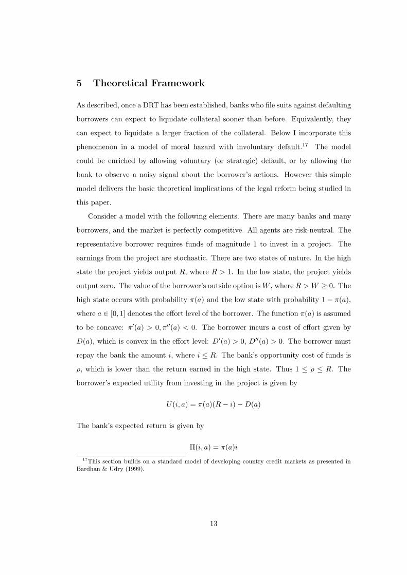
5 Theoretical Framework

As described, once a DRT has been established, banks who file suits against defaulting

borrowers can expect to liquidate collateral sooner than before. Equivalently, they

can expect to liquidate a larger fraction of the collateral. Below I incorporate this

phenomenon in a model of moral hazard with involuntary default.17 The model

could be enriched by allowing voluntary (or strategic) default, or by allowing the

bank to observe a noisy signal about the borrower’s actions. However this simple

model delivers the basic theoretical implications of the legal reform being studied in

this paper.

Consider a model with the following elements. There are many banks and many

borrowers, and the market is perfectly competitive. All agents are risk-neutral. The

representative borrower requires funds of magnitude 1 to invest in a project. The

earnings from the project are stochastic. There are two states of nature. In the high

state the project yields output R, where R > 1. In the low state, the project yields

output zero. The value of the borrower’s outside option is W , where R > W ≥ 0. The

high state occurs with probability π(a) and the low state with probability 1− π(a),

where a ∈ [0, 1] denotes the effort level of the borrower. The function π(a) is assumed

to be concave: π′(a) > 0, π′′(a) < 0. The borrower incurs a cost of effort given by

D(a), which is convex in the effort level: D′(a) > 0, D′′(a) > 0. The borrower must

repay the bank the amount i, where i ≤ R. The bank’s opportunity cost of funds is

ρ, which is lower than the return earned in the high state. Thus 1 ≤ ρ ≤ R. The

borrower’s expected utility from investing in the project is given by

U(i, a) = π(a)(R− i)−D(a)

The bank’s expected return is given by

Π(i, a) = π(a)i17This section builds on a standard model of developing country credit markets as presented in

Bardhan & Udry (1999).

13

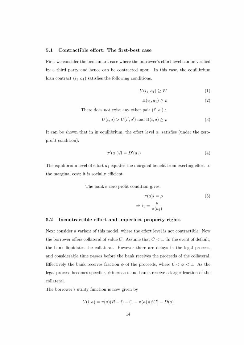
5.1 Contractible effort: The first-best case

First we consider the benchmark case where the borrower’s effort level can be verified

by a third party and hence can be contracted upon. In this case, the equilibrium

loan contract (i1, a1) satisfies the following conditions.

U(i1, a1) ≥ W (1)

Π(i1, a1) ≥ ρ (2)

There does not exist any other pair (i′, a′) :

U(i, a) > U(i′, a′) and Π(i, a) ≥ ρ (3)

It can be shown that in in equilibrium, the effort level a1 satisfies (under the zero-

profit condition):

π′(a1)R = D′(a1) (4)

The equilibrium level of effort a1 equates the marginal benefit from exerting effort to

the marginal cost; it is socially efficient.

The bank’s zero profit condition gives:

π(a)i = ρ (5)

⇒ i1 =ρ

π(a1)

5.2 Incontractible effort and imperfect property rights

Next consider a variant of this model, where the effort level is not contractible. Now

the borrower offers collateral of value C. Assume that C < 1. In the event of default,

the bank liquidates the collateral. However there are delays in the legal process,

and considerable time passes before the bank receives the proceeds of the collateral.

Effectively the bank receives fraction φ of the proceeds, where 0 < φ < 1. As the

legal process becomes speedier, φ increases and banks receive a larger fraction of the

collateral.

The borrower’s utility function is now given by

U(i, a) = π(a)(R− i)− (1− π(a))(φC)−D(a)

14

The bank’s expected return is

Π(i, a) = π(a)i + (1− π(a))(φC)

Since the bank can not contract upon the effort level a, in addition to the three

equilibrium conditions above, the equilibrium (i2, a2) must satisfy an incentive com-

patibility constraint:

a2 = arg maxU(i, a)

Since the borrower’s utility function is differentiable and strictly concave, a necessary

and sufficient condition for this problem is

π′(a2)(R− i2 + φC)−D′(a2) = 0

Therefore, we have

D′(a2) = π′(a2)(R− i2 + φC) (6)

Compare equation (4) with (6). Since i2 > φC, we have that

i2 − φC > 0 ⇒ D′(a2) < D′(a1)

⇒ a2 < a1

The information asymmetry leads the borrower to exert a lower effort level than is

socially efficient. As a result, π(a) is lower, i.e. default is more likely.

Next, from the bank’s zero profit condition we can see that

π(a)i + (1− π(a))φC = ρ (7)

a2 < a1 ⇒ π(a2) < π(a1)

i > φC ⇒ i2 > i1

When the effort level is incontractible, the borrower will charge a higher interest rate

than in the benchmark case. Next, we consider the effects of increased enforceability

of the loan contract, i.e. an increase in the level of φ. The following comparative

statics results follow. The proofs are described in Appendix A.2.

15

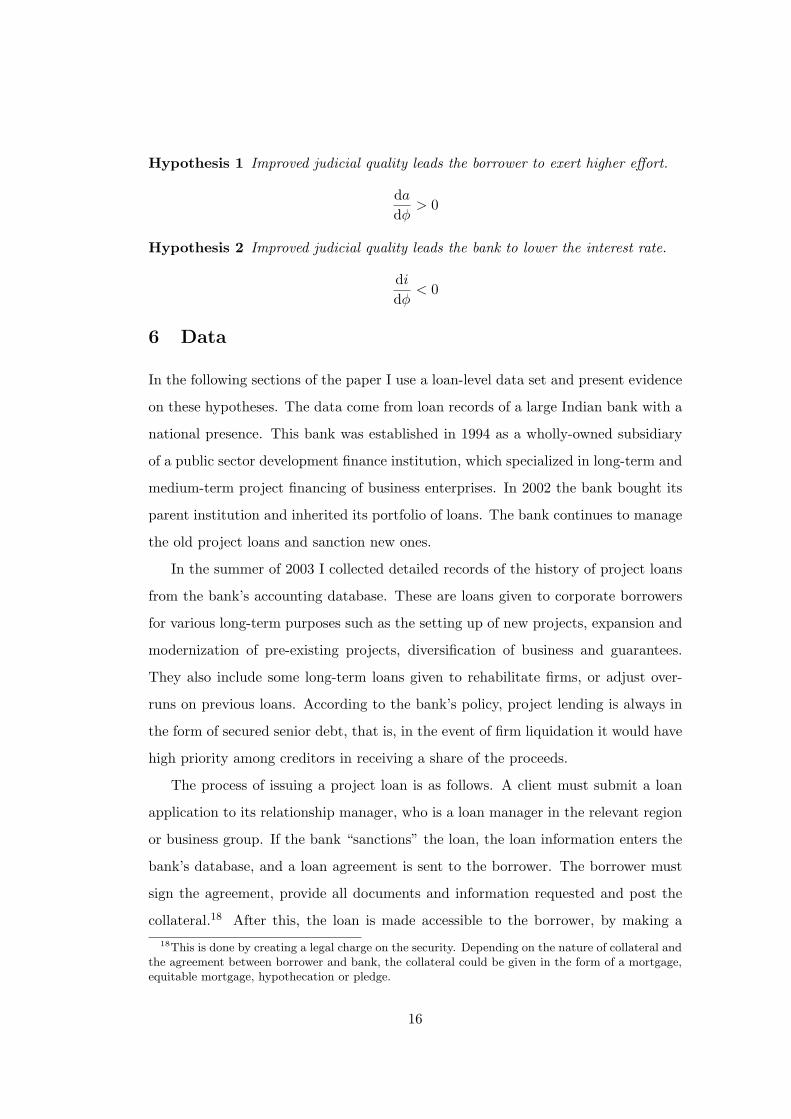
Hypothesis 1 Improved judicial quality leads the borrower to exert higher effort.

da

dφ> 0

Hypothesis 2 Improved judicial quality leads the bank to lower the interest rate.

di

dφ< 0

6 Data

In the following sections of the paper I use a loan-level data set and present evidence

on these hypotheses. The data come from loan records of a large Indian bank with a

national presence. This bank was established in 1994 as a wholly-owned subsidiary

of a public sector development finance institution, which specialized in long-term and

medium-term project financing of business enterprises. In 2002 the bank bought its

parent institution and inherited its portfolio of loans. The bank continues to manage

the old project loans and sanction new ones.

In the summer of 2003 I collected detailed records of the history of project loans

from the bank’s accounting database. These are loans given to corporate borrowers

for various long-term purposes such as the setting up of new projects, expansion and

modernization of pre-existing projects, diversification of business and guarantees.

They also include some long-term loans given to rehabilitate firms, or adjust over-

runs on previous loans. According to the bank’s policy, project lending is always in

the form of secured senior debt, that is, in the event of firm liquidation it would have

high priority among creditors in receiving a share of the proceeds.

The process of issuing a project loan is as follows. A client must submit a loan

application to its relationship manager, who is a loan manager in the relevant region

or business group. If the bank “sanctions” the loan, the loan information enters the

bank’s database, and a loan agreement is sent to the borrower. The borrower must

sign the agreement, provide all documents and information requested and post the

collateral.18 After this, the loan is made accessible to the borrower, by making a18This is done by creating a legal charge on the security. Depending on the nature of collateral and

the agreement between borrower and bank, the collateral could be given in the form of a mortgage,equitable mortgage, hypothecation or pledge.

16

“commitment”.19 (I will use the words “commitment” and “loan” interchangeably

in what follows.) Next, the money is disbursed to the borrower in installments. The

interest rate is determined at the time of the disbursement. Corresponding to each

disbursement is a repayment schedule. After a certain pre-determined moratorium

period has elapsed, the borrower begins to receive bills (known as invoices) from

the bank. Invoices are sent at quarterly intervals. When the borrower sends in a

payment, the amount outstanding is adjusted downwards accordingly. When the

entire invoice amount has been paid, the amount outstanding becomes zero, and the

accounts officer enters the date of final settlement. In the data I observe the detailed

repayment accounts. At each due date in the entire repayment schedule, I know the

amount billed, the amount currently outstanding, and the date of final settlement if

the entire amount has been settled. A positive number outstanding indicates that

the entire amount had not been paid at the time of data collection.

I use this information to calculate for each invoice, how many days elapsed be-

tween the date when the invoice was sent and the date when the payment was received.

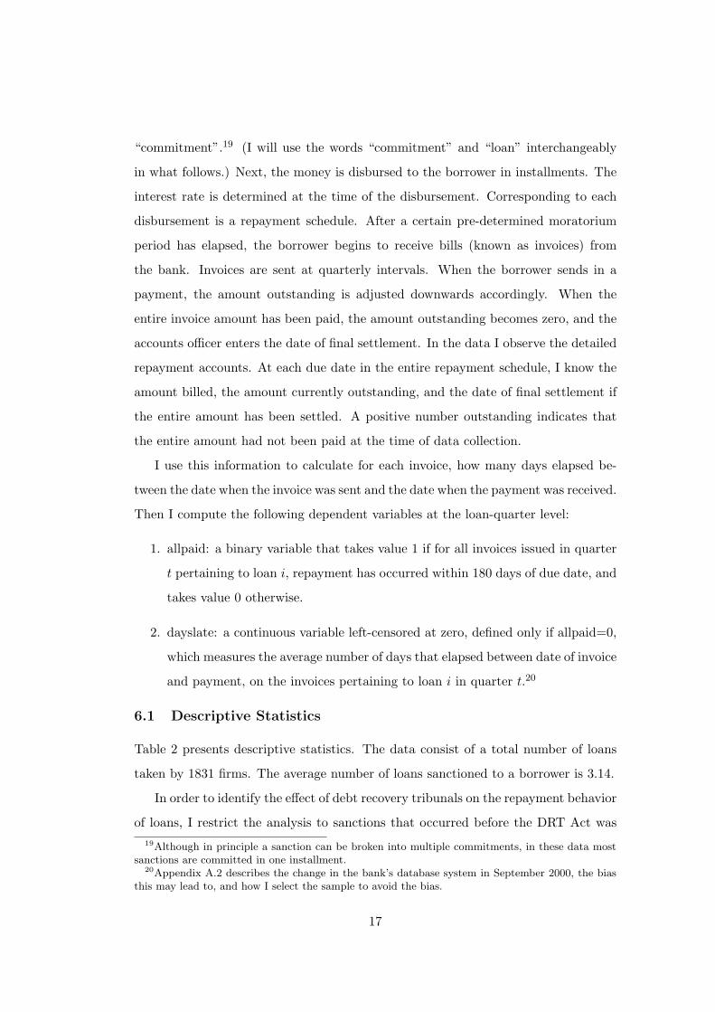
Then I compute the following dependent variables at the loan-quarter level:

1. allpaid: a binary variable that takes value 1 if for all invoices issued in quarter

t pertaining to loan i, repayment has occurred within 180 days of due date, and

takes value 0 otherwise.

2. dayslate: a continuous variable left-censored at zero, defined only if allpaid=0,

which measures the average number of days that elapsed between date of invoice

and payment, on the invoices pertaining to loan i in quarter t.20

6.1 Descriptive Statistics

Table 2 presents descriptive statistics. The data consist of a total number of loans

taken by 1831 firms. The average number of loans sanctioned to a borrower is 3.14.

In order to identify the effect of debt recovery tribunals on the repayment behavior

of loans, I restrict the analysis to sanctions that occurred before the DRT Act was19Although in principle a sanction can be broken into multiple commitments, in these data most

sanctions are committed in one installment.20Appendix A.2 describes the change in the bank’s database system in September 2000, the bias

this may lead to, and how I select the sample to avoid the bias.

17

enforced, i.e. before June 24th, 1993. It is possible that after the DRT Act was

enforced, the pool of borrowers who demanded loans changed or the bank modified

its lending behavior. Hence loans made after this date may be systematically different

from those made before. By restricting the sample in this way I isolate the impact of

this institutional change on repayment behavior on pre-existing loans (moral hazard)

and avoid confounding it with the possibility that new loans are made to better

borrowers (adverse selection).21 This reduces the sample to 798 loans, given to 439

distinct borrowers. The average year of sanction is 1989. The average sanction is for

Rupees 24 million. The majority of loans were issued for new projects. A significant

number of the sanctions were for expansion, modernization and diversification of

plant and machinery. Overruns were another important reason for the sanction. We

observe repayment on commitments for an average of 19 quarters.

The data also confirm that the bank has a national presence. The projects for

which the loans were taken were located in several different states of India. Andhra

Pradesh and Tamil Nadu in the south accounted for 26.2 percent of the loans, Ma-

harashtra and Gujarat in the west accounted for 23.9 percent, Madhya Pradesh in

central India accounted for 7.9, and Rajasthan and Uttar Pradesh in the north ac-

counted for 16.5 percent.

Recall that the prudential norms specify that a loan which has payment overdue

for longer than two quarters (180 days) is non-performing. In 65 percent of the loan-

quarters, invoices are paid up within 180 days. This number varies from 55 percent

in loan-quarters when there is no DRT in the state, to 71 percent when a DRT

does exist. The other dependent variable measures days late, and is only defined for

commitment quarters where not all invoices are paid within 180 days. It is a measure

of how late repayment is, conditional on being late; thus it captures the extent of

delinquency of the delinquent loans. Note that the theoretical predictions for the

two outcome variables are somewhat different. We expect that borrowers respond to

Debt Recovery Tribunals by reducing the probability that they become delinquent on

a loan and therefore increase allpaid. On the other hand, dayslate refers to payments21In Section 8 I relax this restriction and use all the loans, then decompose the effects into moral

hazard and adverse selection.

18

that do not occur on time. In these loan-quarters, borrowers may either have decided

not to pay on time, in which case dayslate may be unaffected by DRTs; or they may

be switching from being late on all loans to paying some loans on time but becoming

more delinquent on others, in which case dayslate could increase; or they may be

attempting to meet the 180 day limit but not succeeding, in which case dayslate

should fall.

7 Empirical Strategy

This section describes the identification strategy and the regressions used to estimate

the effect of Debt Recovery Tribunals.

7.1 Definition of Treatment

A judicial system creates incentives for all entities that fall under its jurisdiction,

even if they do not actually avail of its services. Once a DRT was established in a

location, banks could begin to file debt recovery claims there. Furthermore, once a

DRT is set up, all debt recovery cases with claims above Rupees 1 million pending in

that jurisdiction’s civil courts are required to be transferred to it. Therefore, I define

all loans that fall in the jurisdiction of a DRT as treated in the quarters occurring

after the DRT was established.

I assign loans to DRTs based on the state cluster where the project is located. This

assignment is derived from the rule in the DRT Act, which states that a claim can be

filed in the location where the cause of action arises, or where the defendants reside.

The data on the state of project location is more complete than the information on

borrower location.22

7.2 Estimation and Identification

As described earlier, the empirical strategy in this paper relies on two features of the

DRT Act and its implementation. One is the threshold of Rupees 1 million, since

only claims above this amount can be filed in a Debt Recovery Tribunal. Therefore,

a loan for which more than Rupees 1 million is overdue, is susceptible to have a DRT22Using state of location instead gives qualitatively similar results.

19

case filed against it. The second feature is the timing of tribunal establishment. A

DRT case cannot be filed until there exists a DRT whose jurisdiction this loan falls

under. Different regions received tribunals at different times. This creates variation

at the level of region × time × claim size, which can be utilized to estimate the effect

of DRTs. This is done by estimating the following regression equation:

yijt = β0 + Jj + Tt + β1DRT jt + β2Aboveτ

ij + β3(DRT jt ×Aboveτ

ij) + γXijt + εijt (8)

Here yijt is the dependent variable which measures the time taken to pay the invoices

sent in quarter t for commitment i located in state j, Jj and Tt are vectors of state

and quarter dummies, DRT jt is an indicator for quarters occurring after a DRT was

introduced to state j, and Aboveτij is an indicator for whether an amount larger than

Rupees 1 million was overdue on this sanction at the time when the DRT Act was

enforced (1993:Quarter 2). The vector Xijt represents other borrower and sanction

level controls such as cash flow, year of sanction and the borrower’s industry.

The identification of the effects depends on the exogeneity of the sources of vari-

ation. As discussed earlier, the monetary threshold of Rupees 1 million appears to

have been picked because it was a convenient round number, and does not appear

to have been driven by economic considerations. We might worry that once the

national act was passed in 1993, borrowers may have anticipated that DRT estab-

lishment would follow in the future, and may have sorted their loans to be below the

threshold, by paying up invoices strategically. To avoid this endogenous sorting, the

variable Aboveτij is measured at the time when the DRT Act was enforced, rather

than when the state DRT was established.23

The timing of DRT establishment across states also has a plausibly exogenous

element. As described earlier, initially the government set up DRTs very quickly:

within a space of eight months, five DRTs had been established. The Reserve Bank23One may still be concerned that loans may have sorted endogenously between the time that

borrowers learned of the impending DRT act and it was actually enforced. Note first that the actwas passed within a few months of its introduction in Parliament. Density plots of amount overdueconfirm this (see Figure A.5). In the quarter just before and just after 1993:Q2 the distribution ofloans with amounts above Rupees 1 million overdue did not change significantly. However, even ifthis strategic sorting of loans had occurred, it too would have been an effect of the debt recoverytribunals. Since the bank could file a DRT suit at any time after the DRT was established, to avoidbeing eligible for the DRT the borrower must improve repayment behavior in subsequent quarters.

20

of India’s report on debt recovery tribunals reports that this process received a setback

because of the Delhi High Court’s interim order of 1995 (Reserve Bank of India 1998),

and establishment was interrupted. Without this interruption, it seems likely that

all DRTs would have been established very soon, providing almost no difference in

timing. We may worry that national or state governments may have influenced the

Delhi high court ruling or the Supreme Court stay order. Although both the high

courts and Supreme Court are independent of the executive, it is indeed possible that

state-level opposition to DRTs influenced the Delhi High Court’s decision, or national

level sentiment in favor of such reform influenced the Supreme Court to uphold the

Act. What seems less likely, however, is that the timing of these verdicts could have

been micro-managed by the national government or the states which had not yet

received a DRT.

We may worry also that the timing of DRT establishment was driven by states

lobbying the national government for DRTs at certain times. The time line of DRT

establishment in Appendix A.1 and the map of India in Figure A.1 indicate that the

central government assigned common tribunals to groups of adjacent states (what I

call state clusters). Therefore for DRTs to have been assigned in response to lobbying,

neighboring states would have to have colluded. While this is indeed possible, it would

have been costly and difficult, given that Indian states are distinct geographical and

political entities and often competitors for resources from the national government,

rivals for the use of natural resources, and so on. In Table A.1 (discussed later) I

present results from regressions of the timing of DRT establishment on state-level

factors.

Note also that even if state-level unobservable factors driving repayment behavior

also influenced DRT establishment, there is no a priori reason to believe that they

varied around the Rupees 1 million threshold. Thus if these state-level factors were

common to all loans within the state, then variation in loan repayment behavior

around the Rupees 1 million threshold should only have been introduced by DRTs.

21

8 Results on Repayment Behavior

Here I describe the results from the empirical strategy described above, robustness

checks and further results on the behavioral response to DRTs.

8.1 Main Results

We begin with the results in Table 3A. The sample consists of 15034 observations,

which correspond to loans sanctioned before the DRT Act date. Columns (1)-(4)

correspond to the dependent variable allpaid which measures the probability that

payment on an invoice occurs within 180 days of the invoice date. Columns (5)-

(7) correspond to the dependent variable dayslate, which measures the number of

days that payment takes if allpaid=0. Columns (1) and (5) report the results for

differences-in-differences equation (8), for allpaid and dayslate respectively. The co-

efficient on State DRT × Above corresponds to β3 in equation (8), and is the param-

eter of interest.24 Column (1) shows that when a DRT was established, loans which

had more than Rupees 1 million overdue were 11% more likely to pay up subsequent

invoices within 180 days. Column (5) shows that even loans which did not pay up

within 180 days, did reduce the time taken to pay by 265 days.

Since amount overdue is a continuous variable, it is possible to validate this result

by addressing the following potential concern. Loans with much more than Rupees

1 million overdue might behave systematically differently from those with much less

than Rupees 1 million overdue. Any other state-level changes that coincide with

the establishment of DRTs and affect loans with large dues differentially could be

driving the results in columns (1) and (5). By restricting the sample to loans with

dues close to the 1 million mark, we observe loans which are more homogeneous on all

other dimensions. If DRTs have an impact, then loans with dues just above Rupees

1 million should pay invoices faster that those with dues just below. Therefore, in

columns (2)-(4) and (6)-(7) I estimate the same regression, but only for the sub-

samples that fall within narrow bands around Rupees 1 million. Columns (2) and24Standard errors in Tables 3-5 are block bootstrapped by clusters of states that shared a DRT

to correct for correlated errors within these clusters (Moulton 1990), and serial correlation over time(Bertrand et al. 2004).

22

(6) start with a band of Rupees 1 million ± 150000, i.e. when the amount overdue

falls in the interval [850000, 1150000]. Subsequent bands are narrower sequentially.

Although the standard errors increase due to smaller sample size, the signs of the

coefficients remain the same and the magnitude even increases.

The larger magnitude of the effects in the bands relative to the entire sample,

is interesting. It suggests that loans with much larger amounts overdue reacted less

strongly to the DRTs. When we consider the context of this reform, this seems

plausible. Loans which are highly delinquent may be “too far gone” to respond to

the threat of litigation.

Figures A.2 and A.3 depict these effects with smoothed data. In Figure A.2,

the sample is all loans with amount overdue in the interval [70000, 130000]. The

vertical axis measures the probability that an invoice will be paid within 180 days.

The horizontal axis measures the amount overdue in 1993:Q2 (the potential claim

size). The line with the circles represents allpaid after the state DRT was established,

and that with the triangles represents allpaid before the DRT was established. Note

first that after the DRT is established all loans are more likely to pay invoices on

time. Also, as the amount overdue increases, the probability that an invoice will be

paid on time falls. The two lines are roughly parallel for claim sizes below Rupees

1 million. However as claim size approaches and goes beyond Rupees 1 million the

lines diverge. Before DRTs were established, allpaid continues to fall as amount

overdue increases. However after DRTs were established, loans with claim size above

Rupees 1 million decrease allpaid at a slower rate, flattening out as it approaches

Rs. 1300000. The same phenomenon can be seen by looking at the gap between

these two lines ( A.3). The difference tends to be roughly constant for loans with

claim size below Rupees 1 million but increases as the claim size approaches and

exceeds 1 million. This difference in the change in repayment behavior after DRT

establishment is represented by the results in Table 2A.

8.2 Controlling for Unobservables

A potential concern in using state-level DRT placement to define treatment is whether

time-varying state-level factors could have driven repayment to improve at the same

23

time as DRTs were established. As described above, it appears that the timing of

DRT establishment was driven by interruptions in establishment due to legal chal-

lenges to the act. We may still worry that states could have influenced the placement

of DRTs to some extent. The influence could be correlated with state-level observable

factors or unobservable factors. I examine first if state-level observables can predict

the timing of DRT establishment across states. Table A.1 presents results of this

exercise. I use cross-sectional OLS and probit regressions, as well as fixed effects

regressions where the group variable is the cluster of states which shared a DRT. All

regressions contain year dummies to account for national changes in the probability

that DRTs would be established. To explore the hypothesis that placement is driven

by economic factors, in columns (1)-(4) I alternately include as explanatory variables

state GDP per capita, its growth rate, state credit per capita and its growth rate.

(Note that credit per capita is highly correlated with GDP per capita.) Next I include

the number of cases pending per capita, to test whether states with poor quality ju-

diciaries receive DRTs sooner. On their own, none of these variables appear to affect

the timing of DRT establishment. Next, I include the number of High Court judges

per capita as a measure of the strength of the High Court in a state. I find that when

states have a higher number of judges per capita, the probability of receiving a DRT

is lower. This might be due to a smaller need for a DRT, or because of the opposition

of state high courts to DRTs. Finally, in column (7) I include dummy variables for

the political party of the state government and a dummy variable for whether the

state government was an ally of the party in power at the center.25 None of these

political variables appear to drive the timing of DRT establishment. In column (9)

all variables are included simultaneously in an OLS regression, and in column (10)

in a probit regression. It now appears that the states were more likely to receive a

DRT if they had low numbers of judges per capita, and had an ally of the Janata

party in power. However, once the state clusters are controlled for in the fixed effects

regression (column 11), these variables are no longer significant.25Note that although the period being considered here is only the five years from 1995 to 1999,

the two political variables are not perfectly correlated. During 1995-1999 India had three differentcentral governments. The coalition governments during this period were heavily reliant on supportfrom smaller regional parties, and state political parties are likely to have had considerable influenceon the actions of the central government during this period.

24

Could state-level factors be driving the results in Table 3A? Note first that all

time-invariant state-level factors (observable and unobservable) are controlled for by

putting in state dummies. The fact that loans are only eligible for DRTs if the claim

size is above Rupees 1 million also allows us to control for time-varying state-level un-

observables. Given that the number 1 million appears to have been picked arbitrarily,

there is no reason to believe that these state-level factors would change differentially

for loans with more than Rupees 1 million overdue. In addition, columns (1) and (5)

of Table 2B present an additional check. The regression estimated here is the same

as in Table 2 columns (1) and (5), but with the additional controls of dummies for

state clusters interacted with the quarter. Therefore all factors that change over time

within a state are controlled for. Despite this, in column (1), the coefficient on State

DRT × Above is significant at 9 percent. Thus even after controlling for state-level

unobservables, we continue to find an effect of DRT establishment.

In columns (2) and (6) of Table 3B I address another concern. It could be argued

that borrowers began improving repayment on loans with more than Rupees 1 million

overdue when the national DRT Act was enforced in 1993. Thus a trend could have

begun for loans with dues larger than 1 million to repay faster, and the effect being

picked up by the State DRT× Above variable may actually be a state-level differential

response to the national act. Here I include an additional control, National DRT ×Above. Although loans with more than 1 million overdue did improve repayment

beginning in 1993 as well, the coefficient of State DRT × Above remains at 8 percent

and significant. State DRT establishment has had a robust effect over and above the

national act.

Columns (3) and (7) present an even stricter robustness check. I allow all loans

with dues above 1 million to respond differentially in each quarter. Dummies for

Above interacted with the quarter pick up any nation-wide changes in the behavior

of treated loans from quarter to quarter. If in addition, there is a differential response

across states coincidental with the state DRT establishment, then that response is

very likely to be due to the DRT. In column (3) although the coefficient drops to

0.06, it is still highly significant. In column (7) the magnitude actually increases.

Finally, in columns (4) and (8) I check whether, in states which received a DRT

25

before the 1995 interruption, the response is different from states which received it

after establishment resumed. I call all states that received access to a DRT before

1995, Group 1 states. All other states are Group 2 states.26 In column (4) the

coefficient on Group 2 state × State DRT × Above is not significantly different from

zero, indicating that in levels, the effect of DRTs on allpaid is not different in group 2

states compared to group 1 states. In column (8) we see however, that group 2 state

DRTs have a smaller effect on dayslate than group 1 DRTs. Thus dayslate responds

by less in states which received DRTs after the interruption.

8.3 Behavioral Explanation

Based on results in Table 3A, the average invoice was repaid faster after the state DRT

was set up. Table 2B suggests that this effect was not driven by the national DRT

act, by state-level time-varying unobservables, or by time-varying patterns specific to

loans exposed to DRTs. It also appears that the effect of state DRT on the average

invoice was no different in group 1 states than in group 2 states.

The effect of state DRT on the average invoice does not necessarily tell us whether

individual loans were paid back faster after DRTs than before DRTs. It is possible

that the results in Tables 3A and 3B are driven by compositional changes: invoices

sent out after DRTs were set up might have been for a different set of loans than

invoices sent before. The loan fixed effects results in Table 4 shed light on this issue.

In column (1), the coefficient on State DRT × Above is 0.03 and significant at the

5% level. This can be interpreted as follows. Consider a loan which had more than

Rupees 1 million overdue in 1993. When it received an invoice after the state DRT

was established, it was 3 percent more likely to pay that invoice within 180 days than

one it received before the state DRT was established. The establishment of a DRT

led to improved repayment for the same loan.

In columns (2) and (3) I estimate the same regression within subsets of the sample,

corresponding to observations in group 1 and group 2 states respectively. The results

indicate that in group 1 states, the DRTs do not lead to improved repayment within

loan, however in group 2 states they do. Thus in group 1 states the effect of DRTs26See Appendix A.1 for the time line of DRT establishment across states.

26

was compositional, but in group 2 states individual loans were affected. This is borne

out in the borrower fixed effects results as well (columns 4-6): in group 2 states the

same borrower paid back loans faster after DRTs were established.

It is not easy to understand why this is the case. However it is consistent with the

earlier discussion on the Supreme Court’s 1996 ruling overturning the verdict of the

Delhi High Court. By ruling that DRTs should resume their functions, the Supreme

Court may have suggested that it would uphold the act. Borrowers in group 2 states

might have responded to DRTs more strongly than those in group 1 states.

9 Results on Future Lending Behavior

Next I ask if the contractual terms of the new loans issued after DRTs were established

are significantly different from those issued before. Specifically, I consider the size of

the sanction and the interest rate. The identification strategy is different from the

one employed in the previous sections: the analysis relies on the differential timing

of DRT establishment across states. The regression estimated is of the form:

yijt = β0 + Jj + Tt + β1DRT jt + γXijt + εijt (9)

Here yijt measures either the size of the sanction or the interest rate on the

disbursement. The right hand side include state dummies, year dummies and controls

at the loan level as well as borrower level. The coefficient of interest β1 which captures

the effect of state DRT establishment. Note here that identification relies on the

exogeneity of the timing of DRT placement across states.

9.1 Size of loan sanctioned

The model described in section 4 could be extended to allow for a variable size of

investment, say L. Then if we assume that output is a concave function of loan size,

R = R(L) where R′ > 0, R′′ < 0, then the complementarity between effort and invest-

ment may lead to under-investment. As the borrower’s loan size and consequently

debt burden increases, his benefit from the high state of nature decreases. Due to

limited liability, his loss from the low state remains constant at zero. Therefore he is

more likely to default. This makes each additional unit of lending more costly to the

27

bank and so the loan size may be capped at a sub-optimal level (known as micro-

rationing; Bardhan & Udry 1999). An increase in judicial quality will increase the

value of the collateral to the bank and hence increase its gains from the high state.

This may induce the bank to increase the size of the loan offered. Additionally, larger

loans are more likely to fall over the Rs. 1 million overdues threshold and therefore

potentially treated by DRTs. Therefore banks may become more likely to offer them.

On the other hand, borrowers may prefer smaller loans precisely to avoid this threat

of DRTs. Therefore the net effect of the reform is not easy to predict. It is tested

empirically in Table 5.

The observations in this Table (and in Table 6) consist of all loans in the sam-

ple, i.e. loans sanctioned before the DRT Act as well as after. In columns (1)-(3)

I estimate cross-sectional regressions and in columns (4)-(6) borrower fixed effects

regressions. The dependent variable is the logarithm of loan size. In all regressions

I control for state dummies, year dummies, type of project for which the loan was

taken, currency of loan and state of project location. In addition in the cross-sectional

regressions I control for the firm’s industry, and its asset size. As we see, the effect of

state DRT establishment is not significantly different from zero in any of the columns.

It appears that the reform has not led to larger loan size.27

9.2 Interest rates

In Table 6, I test the model’s prediction for interest rates: when contract enforcement

improves, the equilibrium interest rate decreases. Once again I start with cross-

sectional regressions and then move to borrower fixed effects. Since the interest rate

is determined at the time of disbursement, an observation here is a disbursement.

The dependent variable is the interest rate on the disbursement. In all columns the

same covariates are controlled for as in Table 5; in addition I also control for the size

of the loan and the timing of the sanction and commitment.

In column (1) it appears that the establishment of DRTs caused loans sanctioned

subsequently to charge an interest rate that is 2.2 percentage points lower than loans27Figure A.4 plots the coefficients on Post state DRT for decile regressions, together with the

point-wise confidence interval. The coefficient is not significantly different from zero in any of thedeciles.

28

sanctioned before. National changes in the interest rate are controlled for with year

dummies. However, just as before, we may worry that interest rates in different states

responded differently to the national DRT act. So in column (2) I put in a dummy for

observations occurring after 1993 Quarter 2. The national-level decrease in interest

rates is not significant, and it does not change the coefficient on state DRT. Column

(3) shows that in group 1 states the interest rate decreased by 2.7 percentage points,

whereas in group 2 states it decreased by a smaller 1.4 percentage points.

In the borrower fixed effects regressions (columns 4-6), the results are not signif-

icant. That is, when we look at borrowers who received loans both before and after,

they do not seem to receive lower interest rates after the DRTs were set up. This could

be for a variety of reasons. Repeat borrowers are a select group of borrowers who

probably get repeated loans because they have proved their creditworthiness. The

DRTs appears to have done little to enhance the creditworthiness of these higher-

quality borrowers. Thus the average new borrower who gets a loan after the state

DRT may get a cheaper loan than the average borrower before the DRT, but the

repeat borrower may already be receiving a cheaper loan, which does not become

even cheaper after DRTs are established.

Finally, there is the question of what the lower interest rates on the average new

loan signifies. I do not observe loan applications which are not approved by the bank.

Therefore it is not possible to separate the effects of this reform on the demand versus

the supply of loans. Furthermore, we cannot infer the supply of credit to borrowers

who do not get project loans after the reform. One may worry also that new loans

are given for less risky projects than before, which allows interest rates to be lower.

In all regressions in Table 6, I control for observable characteristics of the loans that

may be correlated with riskiness: borrower industry, type of project, and size of loan.

However to the extent that the riskiness of a project is unobservable, it cannot be

controlled for.

There is also the question of the effect of this reform on credit throughout the

banking system. To interpret this as a move down the demand curve for credit, we

need evidence not just on interest rates but also on the volume of credit. We have

found no evidence of increase in average loan size given by this bank, in this loan

29

category. It is in principle possible that as these loans became cheaper, other loans

unaffected by DRTs became more expensive instead. This burden may have fallen

on the same class of borrowers if they also use these loans, or on an entirely different

set of borrowers. Unfortunately I do not have data on all loans given by this bank,

or all loans in the banking system in general. Therefore it is outside the scope of this

paper to analyze these effects.

10 Conclusion

This paper has used a micro data set on project loans to examine the effect of a

reform aimed at speeding up the legal process to resolve disputes between banks

and defaulting borrowers. The results show that the establishment of the new Debt

Recovery Tribunals reduces delinquency by 3-11 percent. Furthermore, new loans

sanctioned after DRT establishment are charged interest rates that are lower by 1.4-

2 percentage points.

The type of judicial reform studied here is relevant for developing economies for

various reasons. Debt Recovery Tribunals were established as the Indian govern-

ment’s attempt to improve the legal channels for loan recovery, without overhauling

the entire judicial system. By accommodating the opposition without diluting the

intent of the act, the government successfully implemented the reform. This is a

reasonable representation of judicial reform as it might be carried out in developing

countries.

Descriptive evidence suggests that these DRTs have reduced the time taken to

process debt recovery cases. The results indicate that they have also led to re-

duced delinquency in loan repayment. Given that banks in several emerging market

economies have high volumes of non-performing loans such judicial reform can have

important consequences. As these economies transition towards greater reliance on

market forces, the banks rely on the legal and judicial framework to enforce contracts.

Since bank credit tends to form a large share of total credit in these economies, the

performance of the banking sector has implications for macroeconomic stability. It

has also been argued that financial depth is important for economic growthKing &

Levine (1993). By improving the efficiency of banking intermediation such reform

30

can promote higher growth rates for these economies.

This paper also demonstrates a mechanism through which this reform may affect

the credit market. The establishment of DRTs appears to have led this bank to

charge lower interest rates on new project loans, holding constant inter alia type of

project, borrower industry, project location, and size of loan. If these new projects

are not different from previous ones in terms of riskiness, then this can be interpreted

as a cheapening of credit, which is likely to spur entrepreneurial activity.

31

References

Acemoglu, Daron, Johnson, Simon, & Robinson, David. 2001. The Colonial Origins

of Comparative Development: An Empirical Investigation. American Economic

Review, 91, 1369–1401.

Banerjee, Abhijit, & Iyer, Lakshmi. 2003. History, Institutions and Economic Perfor-

mance: The Legacy of Colonial Land Tenure Systems in India. BREAD Working

Paper Number 003.

Bardhan, Pranab, & Udry, Christopher. 1999. Development Microeconomics. New

York: Oxford University Press.

Bertrand, Marianne, Duflo, Esther, & Mullainathan, Sendhil. 2004. How Much

Should We Trust Differences-in-Differences Estimates? Quarterly Journal of Eco-

nomics, 119(1), 249–275.

Demirguc-Kunt, Asli, & Maksimovic, Vojislav. 1998. Law, Finance and Firm Growth.

Journal of Finance, 53(6), 2107–2137.

Djankov, Simeon, Porta, Rafael La, de Silanes, Florencio Lopez, & Shleifer, Andrei.

2003. Courts. Quarterly Journal of Economics, 118(2), 452–517.

Government of India. 1991. Report of the Narasimham Committee on the Financial

System. New Delhi: Nabhi Publications. Reprint.

Government of India. 2003. Statement Showing Number of Cases Filed, Number of

Cases Disposed of, Amount Involved & Amount Recovered. Delhi: Ministry of

Finance.

King, Robert G., & Levine, Ross. 1993. Finance and Growth: Schumpeter Might be

Right. Quarterly Journal of Economics, 108(3), 717–738.

Kohling, Wolfgang. 2002. Implications of India’s Judicial System for Economic and

Agricultural Growth and Poverty Reduction. Hamburg: Books on Demand.

La Porta, Rafael, Lopez-de-Silanes, Florencio, Shleifer, Andrei, & Vishny, Robert.

1998. Law and Finance. Journal of Political Economy, 106(6), 1113–1155.

32

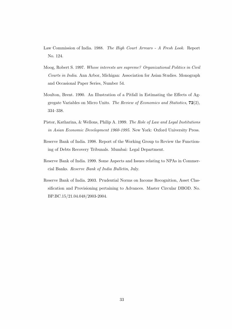
Law Commission of India. 1988. The High Court Arrears - A Fresh Look. Report

No. 124.

Moog, Robert S. 1997. Whose interests are supreme? Organizational Politics in Civil

Courts in India. Ann Arbor, Michigan: Association for Asian Studies. Monograph

and Occasional Paper Series, Number 54.

Moulton, Brent. 1990. An Illustration of a Pitfall in Estimating the Effects of Ag-

gregate Variables on Micro Units. The Review of Economics and Statistics, 72(2),

334–338.

Pistor, Katharina, & Wellons, Philip A. 1999. The Role of Law and Legal Institutions

in Asian Economic Development 1960-1995. New York: Oxford University Press.

Reserve Bank of India. 1998. Report of the Working Group to Review the Function-

ing of Debts Recovery Tribunals. Mumbai: Legal Department.

Reserve Bank of India. 1999. Some Aspects and Issues relating to NPAs in Commer-

cial Banks. Reserve Bank of India Bulletin, July.

Reserve Bank of India. 2003. Prudential Norms on Income Recognition, Asset Clas-

sification and Provisioning pertaining to Advances. Master Circular DBOD. No.

BP.BC.15/21.04.048/2003-2004.

33

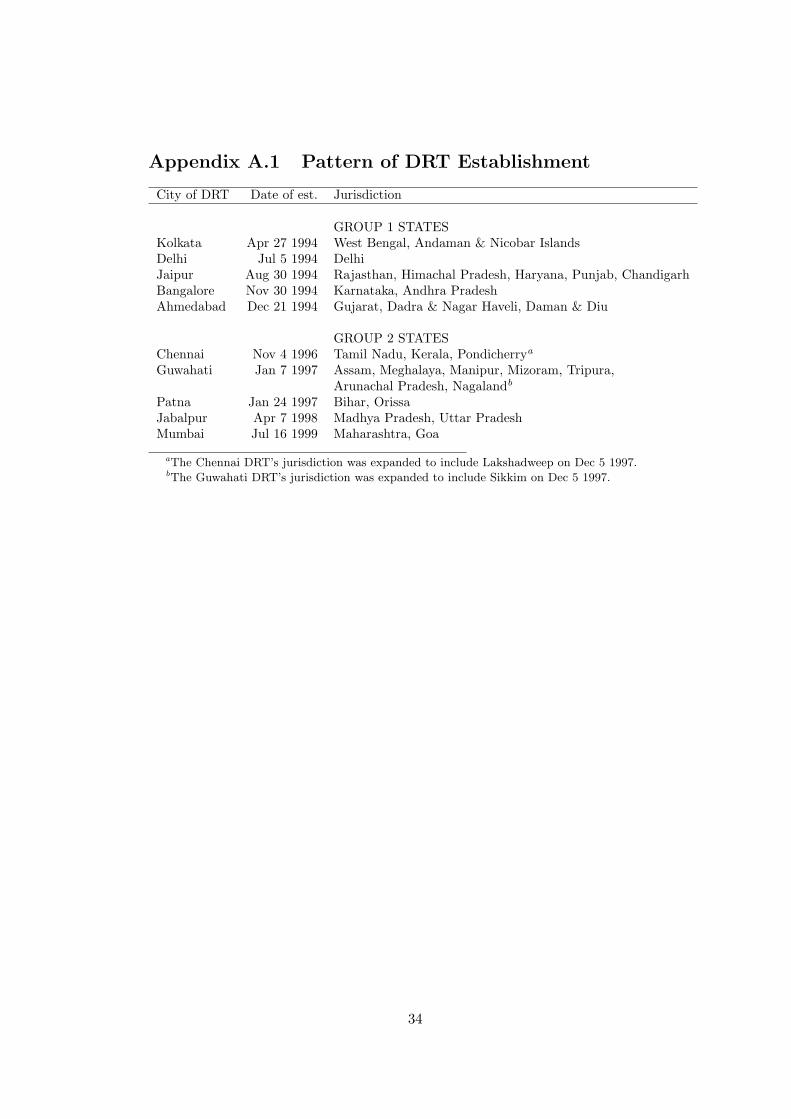
Appendix A.1 Pattern of DRT Establishment

City of DRT Date of est. Jurisdiction

GROUP 1 STATESKolkata Apr 27 1994 West Bengal, Andaman & Nicobar IslandsDelhi Jul 5 1994 DelhiJaipur Aug 30 1994 Rajasthan, Himachal Pradesh, Haryana, Punjab, ChandigarhBangalore Nov 30 1994 Karnataka, Andhra PradeshAhmedabad Dec 21 1994 Gujarat, Dadra & Nagar Haveli, Daman & Diu

GROUP 2 STATESChennai Nov 4 1996 Tamil Nadu, Kerala, Pondicherrya

Guwahati Jan 7 1997 Assam, Meghalaya, Manipur, Mizoram, Tripura,Arunachal Pradesh, Nagalandb

Patna Jan 24 1997 Bihar, OrissaJabalpur Apr 7 1998 Madhya Pradesh, Uttar PradeshMumbai Jul 16 1999 Maharashtra, Goa

aThe Chennai DRT’s jurisdiction was expanded to include Lakshadweep on Dec 5 1997.bThe Guwahati DRT’s jurisdiction was expanded to include Sikkim on Dec 5 1997.

34

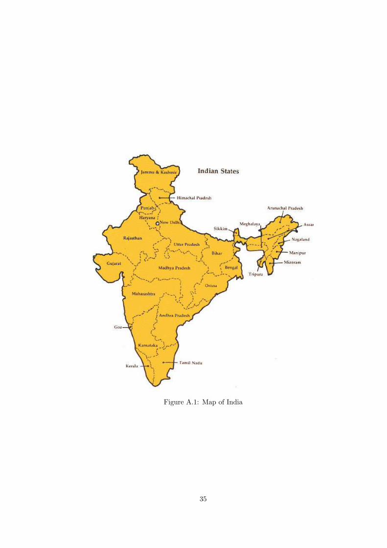
Figure A.1: Map of India

35

Appendix A.2 Proof of Hypotheses

Hypothesis 1

The equilibrium condition (6) is

D′(a2) = π′(a2)(R− i2 + φC)

⇒ π′(a2)D′(a2)

=1

R− i2 + φC

When φ increases, the left hand side of this equation must decrease.Since π′′(a) < 0 and D′′(a) > 0, this requires that a should increase.

Hypothesis 2

The bank’s zero profit condition (7) gives us

i =ρ− φC + π(a)φC

π(a)

Therefore,

di

dφ=

π(a) dadφ [−(1− π(a))C + π′(a)φC]− π′(a) da

dφ [ρ− (1− π(a))φC]

[π(a)]2

We know that C < 1 ≤ ρ. This gives us

di

dφ< 0.

36

Appendix A.3 Data Cleaning

Database Transfer

In September 2000, the bank moved its project loan database from an old database systemto a new one. Only loans that were active at the time of migration were transferred to thenew system. All loans sanctioned after the date of migration are in the new system. For anyactive loan the entire repayment schedule is available and hence can be used to reconstructthe history of repayment as described above. My data consist of all loans that existed in thenew database at the time of data collection (May 2003), currently active or not. However,the removal of currently inactive loans at the time of database migration causes the followingproblem due to systematic attrition in the data.The objective of this paper is to examine delinquency, or delays in loan repayment. If a loanis delinquent, the account will remain active for longer since the bank will employ variousmethods to obtain the payment until the payment is made, or else the loan is writtenoff the books. Therefore at any point in time if we look only at active loans, they aredisproportionately likely to be delinquent. Thus the loans transferred to the new system arelikely to have disproportionately large number of delinquent loans. However we observe theentire population of loans sanctioned after the database migration, thus these loans havethe correct proportion of delinquent loans. This biases the data in favor of finding thatdelinquency has decreased over time.To remove this problem, I restrict my sample to loans whose last invoice date was scheduledto occur after the date of migration. Barring pre-payment, all of these loans would have tobe in the new database regardless of past performance.a

Survival

The snapshot nature of the data also introduce the issue of survival probabilities. Whencomputing the variable dayslate for invoices that were not repaid by the time of data collec-tion I can only say that repayment is at least x number of days late, but cannot accuratelymeasure the actual number of days late. Since newer loans begin issuing invoices later in thetime period, the variable dayslate will tend to show that their payment is less late than forolder loans. In all specifications I include the year of sanction as a control. In addition topicking up cohort effects, it controls for the problem that newer sanctions that are delinquenthave systematically different dayslate than older delinquent sanctions.

aAmong the loans sanctioned since the date of migration, very few invoices are pre-paid. Thissuggests that the absence of prepaid invoices should not bias the results appreciably.

37

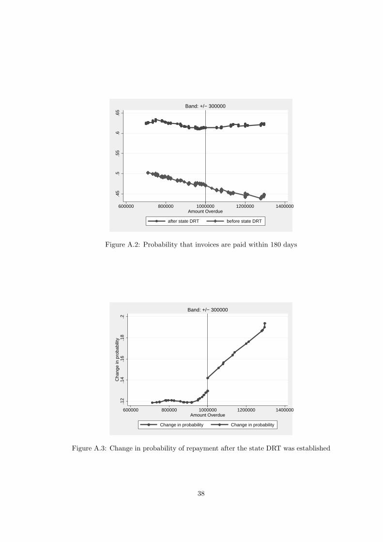
.45

.5.5

5.6

.65

600000 800000 1000000 1200000 1400000Amount Overdue

after state DRT before state DRT

Band: +/− 300000

Figure A.2: Probability that invoices are paid within 180 days

.12

.14

.16

.18

.2C

hang

e in

pro

babi

lity

600000 800000 1000000 1200000 1400000Amount Overdue

Change in probability Change in probability

Band: +/− 300000

Figure A.3: Change in probability of repayment after the state DRT was established

38

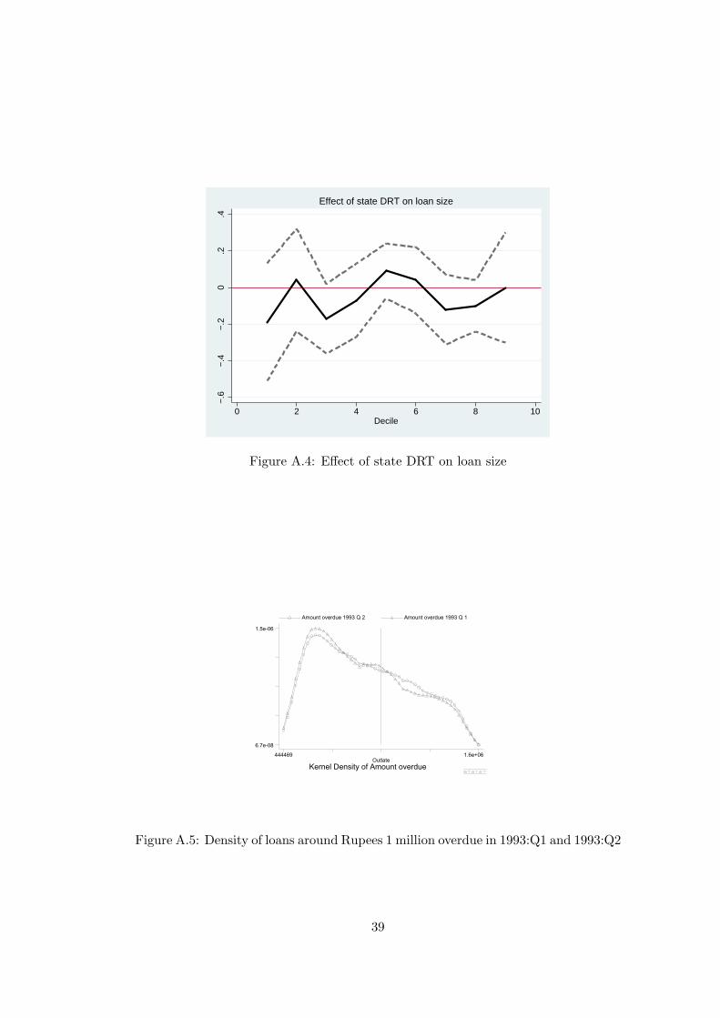
−.6

−.4

−.2

0.2

.4

0 2 4 6 8 10Decile

Effect of state DRT on loan size

Figure A.4: Effect of state DRT on loan size

Kernel Density of Amount overdueOutlate

Amount overdue 1993 Q 2 Amount overdue 1993 Q 1

444469 1.6e+06

6.7e-08

1.5e-06

Figure A.5: Density of loans around Rupees 1 million overdue in 1993:Q1 and 1993:Q2

39

Table 1: Summary statistics about case processing in Bombay High Court versus Mumbai DRTs Filed in HC Filed in DRT Number 18 32 File date Mean January 1997 August 2002 Median March 1998 May 2003 Claim size Mean Rs. 820 million Rs. 189 million Median Rs. 120 million Rs. 126 million Time to summons 393 days 136 days (916 days) (244 days) Time to first hearing 335 days 211 days (687) (295) Time to applicant’s evidence 2628 days 802 days (775) (457) Time to defendant’s evidence 2981 days 696 days (794) (153) Time to arguments starting 2623 days 1095 days (557) (548) Interim relief granted (probability) 0.67 0.47 (0.49) (0.51) Type of resolution (percentages) Recovery certificate 27.8 18.8 Consent decree 0.0 9.4 Settled 16.7 3.1 Hearings on 38.9 28.1 Stuck at BIFR 16.7 24.4 In appeal at higher forum 0.0 6.3 Finished (percentages) 44.4 31.3 Standard errors in parentheses.

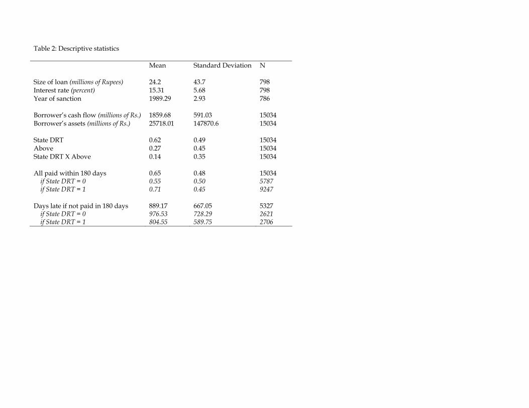
Table 2: Descriptive statistics Mean Standard Deviation N Size of loan (millions of Rupees) 24.2 43.7 798 Interest rate (percent) 15.31 5.68 798 Year of sanction 1989.29 2.93 786 Borrower’s cash flow (millions of Rs.) 1859.68 591.03 15034 Borrower’s assets (millions of Rs.) 25718.01 147870.6 15034 State DRT 0.62 0.49 15034 Above 0.27 0.45 15034 State DRT X Above 0.14 0.35 15034 All paid within 180 days 0.65 0.48 15034 if State DRT = 0 0.55 0.50 5787 if State DRT = 1 0.71 0.45 9247 Days late if not paid in 180 days 889.17 667.05 5327 if State DRT = 0 976.53 728.29 2621 if State DRT = 1 804.55 589.75 2706

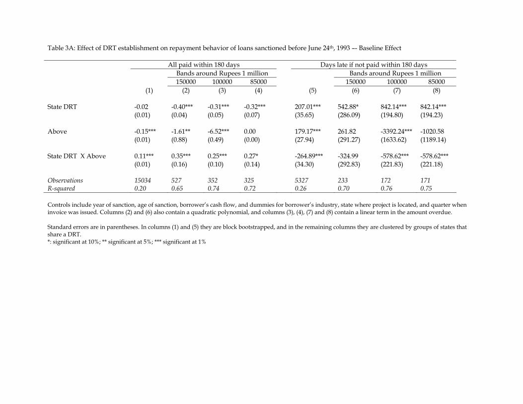
Table 3A: Effect of DRT establishment on repayment behavior of loans sanctioned before June 24th, 1993 –- Baseline Effect

All paid within 180 days Days late if not paid within 180 days Bands around Rupees 1 million Bands around Rupees 1 million 150000 100000 85000 150000 100000 85000 (1) (2) (3) (4) (5) (6) (7) (8)

State DRT -0.02 -0.40*** -0.31*** -0.32*** 207.01*** 542.88* 842.14*** 842.14*** (0.01) (0.04) (0.05) (0.07) (35.65) (286.09) (194.80) (194.23) Above -0.15*** -1.61** -6.52*** 0.00 179.17*** 261.82 -3392.24*** -1020.58 (0.01) (0.88) (0.49) (0.00) (27.94) (291.27) (1633.62) (1189.14) State DRT X Above 0.11*** 0.35*** 0.25*** 0.27* -264.89*** -324.99 -578.62*** -578.62*** (0.01) (0.16) (0.10) (0.14) (34.30) (292.83) (221.83) (221.18) Observations 15034 527 352 325 5327 233 172 171 R-squared 0.20 0.65 0.74 0.72 0.26 0.70 0.76 0.75 Controls include year of sanction, age of sanction, borrower’s cash flow, and dummies for borrower’s industry, state where project is located, and quarter when invoice was issued. Columns (2) and (6) also contain a quadratic polynomial, and columns (3), (4), (7) and (8) contain a linear term in the amount overdue. Standard errors are in parentheses. In columns (1) and (5) they are block bootstrapped, and in the remaining columns they are clustered by groups of states that share a DRT. *: significant at 10%; ** significant at 5%; *** significant at 1%

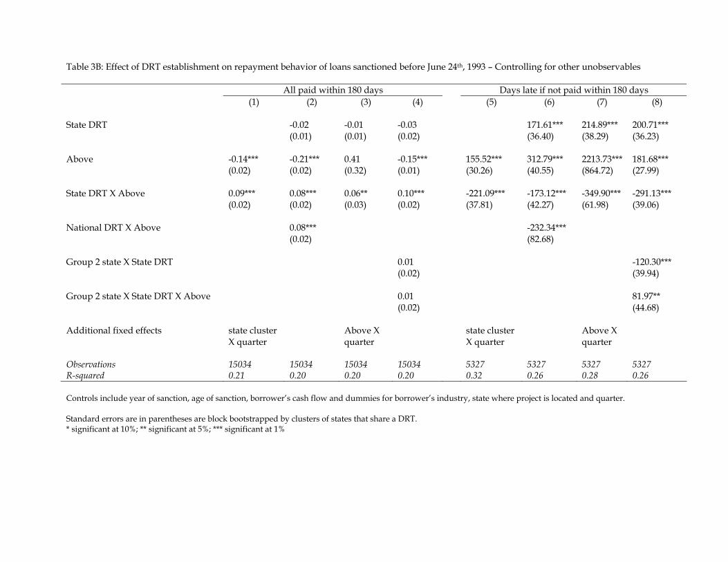
Table 3B: Effect of DRT establishment on repayment behavior of loans sanctioned before June 24th, 1993 – Controlling for other unobservables All paid within 180 days Days late if not paid within 180 days

(1) (2) (3) (4) (5) (6) (7) (8) State DRT -0.02 -0.01 -0.03 171.61*** 214.89*** 200.71*** (0.01) (0.01) (0.02) (36.40) (38.29) (36.23) Above -0.14*** -0.21*** 0.41 -0.15*** 155.52*** 312.79*** 2213.73*** 181.68*** (0.02) (0.02) (0.32) (0.01) (30.26) (40.55) (864.72) (27.99) State DRT X Above 0.09*** 0.08*** 0.06** 0.10*** -221.09*** -173.12*** -349.90*** -291.13*** (0.02) (0.02) (0.03) (0.02) (37.81) (42.27) (61.98) (39.06) National DRT X Above 0.08*** -232.34*** (0.02) (82.68) Group 2 state X State DRT 0.01 -120.30*** (0.02) (39.94) Group 2 state X State DRT X Above 0.01 81.97** (0.02) (44.68) Additional fixed effects state cluster

X quarter Above X

quarter state cluster

X quarter Above X

quarter

Observations 15034 15034 15034 15034 5327 5327 5327 5327 R-squared 0.21 0.20 0.20 0.20 0.32 0.26 0.28 0.26 Controls include year of sanction, age of sanction, borrower’s cash flow and dummies for borrower’s industry, state where project is located and quarter. Standard errors are in parentheses are block bootstrapped by clusters of states that share a DRT. * significant at 10%; ** significant at 5%; *** significant at 1%

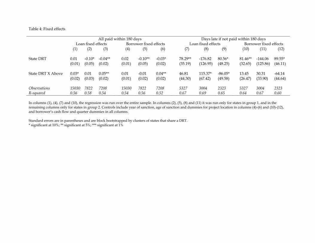
Table 4: Fixed effects

All paid within 180 days Days late if not paid within 180 days Loan fixed effects Borrower fixed effects Loan fixed effects Borrower fixed effects (1) (2) (3) (4) (5) (6) (7) (8) (9) (10) (11) (12)

State DRT 0.01 -0.10* -0.04** 0.02 -0.10** -0.03* 78.29** -176.82 80.56* 81.46** -144.06 89.55* (0.01) (0.05) (0.02) (0.01) (0.05) (0.02) (35.19) (126.95) (48.25) (32.65) (125.86) (46.11) State DRT X Above 0.03* 0.01 0.05** 0.01 -0.01 0.04** 46.81 115.37* -86.05* 13.45 30.31 -64.14 (0.02) (0.03) (0.02) (0.01) (0.02) (0.02) (44.30) (67.42) (49.58) (26.47) (33.90) (44.64) Observations 15030 7822 7208 15030 7822 7208 5327 3004 2323 5327 3004 2323 R-squared 0.56 0.58 0.54 0.54 0.56 0.52 0.67 0.69 0.65 0.64 0.67 0.60 In columns (1), (4), (7) and (10), the regression was run over the entire sample. In columns (2), (5), (8) and (11) it was run only for states in group 1, and in the remaining columns only for states in group 2. Controls include year of sanction, age of sanction and dummies for project location in columns (4)-(6) and (10)-(12), and borrower’s cash flow and quarter dummies in all columns. Standard errors are in parentheses and are block bootstrapped by clusters of states that share a DRT. * significant at 10%; ** significant at 5%; *** significant at 1%

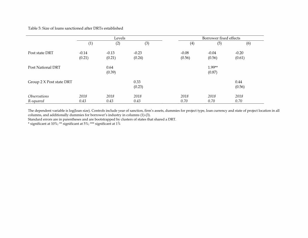
Table 5: Size of loans sanctioned after DRTs established Levels Borrower fixed effects

(1) (2) (3) (4) (5) (6) Post state DRT -0.14 -0.13 -0.23 -0.08 -0.04 -0.20 (0.21) (0.21) (0.24) (0.56) (0.56) (0.61) Post National DRT 0.64 1.99** (0.39) (0.87) Group 2 X Post state DRT 0.33 0.44 (0.23) (0.56) Observations 2018 2018 2018 2018 2018 2018 R-squared 0.43 0.43 0.43 0.70 0.70 0.70 The dependent variable is log(loan size). Controls include year of sanction, firm’s assets, dummies for project type, loan currency and state of project location in all columns, and additionally dummies for borrower’s industry in columns (1)-(3). Standard errors are in parentheses and are bootstrapped by clusters of states that shared a DRT. * significant at 10%; ** significant at 5%; *** significant at 1%

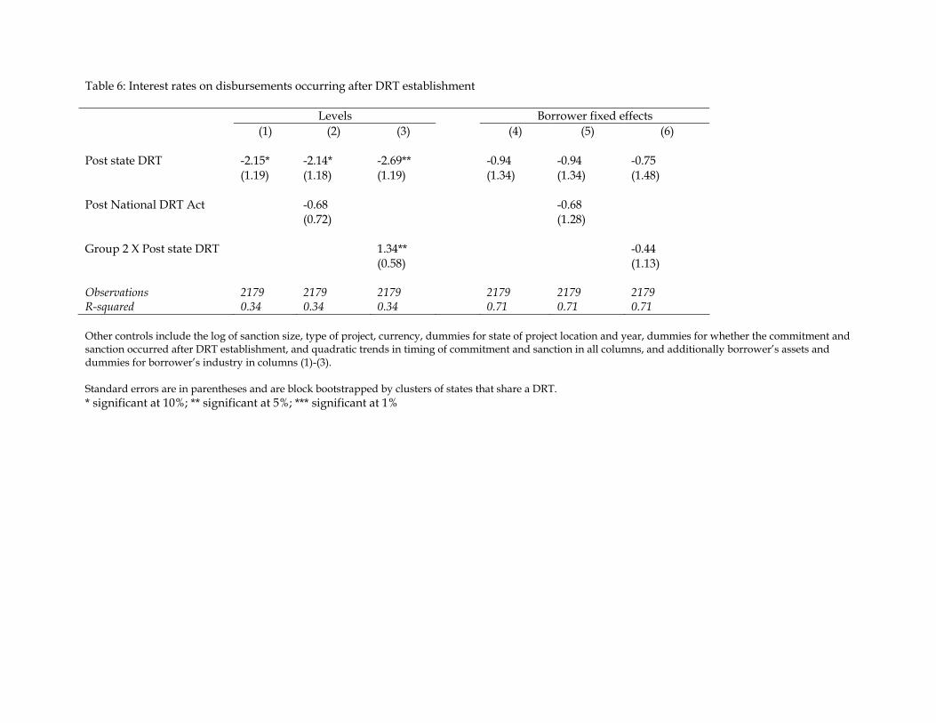
Table 6: Interest rates on disbursements occurring after DRT establishment

Levels Borrower fixed effects (1) (2) (3) (4) (5) (6)

Post state DRT -2.15* -2.14* -2.69** -0.94 -0.94 -0.75 (1.19) (1.18) (1.19) (1.34) (1.34) (1.48) Post National DRT Act -0.68 -0.68 (0.72) (1.28) Group 2 X Post state DRT 1.34** -0.44 (0.58) (1.13) Observations 2179 2179 2179 2179 2179 2179 R-squared 0.34 0.34 0.34 0.71 0.71 0.71 Other controls include the log of sanction size, type of project, currency, dummies for state of project location and year, dummies for whether the commitment and sanction occurred after DRT establishment, and quadratic trends in timing of commitment and sanction in all columns, and additionally borrower’s assets and dummies for borrower’s industry in columns (1)-(3). Standard errors are in parentheses and are block bootstrapped by clusters of states that share a DRT. * significant at 10%; ** significant at 5%; *** significant at 1%

Table A.1: Predicting the pattern of DRT incidence, dependent variable = 1 if state i had a debt recovery tribunal in year t.

Cross-sectional OLS Probit Court FE (1) (2) (3) (4) (5) (6) (7) (8) (9) (10) (11) GDP per capita -0.05

(0.05) GDP growth rate -0.00 0.00 0.04 -0.00 (0.00) (0.00) (0.03) (0.00) Credit per capita -0.00 (0.00) Credit growth rate -0.00 (0.00) Cases pending per capita 0.00 0.00 0.08 -0.01 (0.00) (0.01) (0.08) (0.03) Judges per capita -9.28** -10.75** -81.39*** -4.22 (3.74) (4.80) (29.41) (5.85) State government Congress & allies 0.00 0.09 0.75 0.05 (0.07) (0.09) (0.60) (0.09) Janata & allies 0.09 0.11 1.39** 0.06 (0.08) (0.10) (0.68) (0.13) Communist party 0.11 0.12 1.09 0.06 (0.08) (0.09) (0.68) (0.12) Regional party 0.10 0.11 0.95 -0.02 (0.07) (0.09) (0.58) (0.13) Center’s ally -0.07 -0.03 -0.54 -0.06 (0.05) (0.07) (0.48) (0.07) Observations 192 168 192 192 192 192 192 192 168 96 168 R-squared 0.73 0.68 0.72 0.72 0.72 0.74 0.73 0.73 0.71 0.41a 0.79

Robust standard errors in parentheses. Year dummies in all columns not reported. Observations correspond to 8 years of data (1993-2000) for 24 states. GDP growth rates are not available for 1993. Union territories are excluded. The court fixed effects regression is run for groups of states which share a high court. * significant at 10%; ** significant at 5%; *** significant at 1%. a: Pseudo R-squared.