Latin American Journal of Central Banking 3 (2022) 100048

Contents lists available at ScienceDirect

Latin American Journal of Central Banking

journal homepage: www.elsevier.com/locate/latcb

Price, sales, and the business cycle: Microeconomic evidence

☆

Fernando Borraz a , ∗ , Giacomo Livan

b , Anahí Rodríguez-Martínez c , Pablo Picardo

d

a Banco Central del Uruguay, Departamento de Economía de la Facultad de Ciencias Sociales de la Universidad de la República and Universidad de

Montevideo, Uruguay b University College London, UK c Centro de Estudios Monetarios Latinoamericanos, Uruguay d Banco Central del Uruguay, Uruguay

a r t i c l e i n f o

JEL classification:

E31 E32 E24 C38

Keywords:

Price rigidity Sales Unemployment Time series principal component analysis

a b s t r a c t

This paper uses a rich weekly price database from the largest supermarket in Uruguay to ana- lyze the relationship among prices, micro-level sales, and business cycle conditions. On average, 7% of products were on sale each month, and we show a positive and statistically significant but small relationship between sales and unemployment at the aggregate level, controlling for product and time effects. For each product category, there is a high and positive statistically sig- nificant association for these variables. Also, for some categories like food products, alcoholic drinks, beverages, and fruits and vegetables, we found a large, negative, and statistically signifi- cant relationship between the probability of being on sale and employment. The mechanism we tested is the following: As the economy worsens and unemployment rises (and/or employment falls), the supermarket uses sales to adjust prices while keeping reference prices fixed. Our results indicate that sales do not alleviate much of the price rigidity in economic recessions.

We also studied sales behavior through a principal component analysis in the time domain. This analysis revealed that the first two principal components explained more than half of each sector’s variance in price dynamics. These components are significantly correlated with varia- tions in unemployment and employment. Additionally, we found that movement in the principal components across sectors systematically Granger-cause employment changes.

1. Introduction

Departing from the works of Lucas (1972) , Taylor (1979, 1980) , and Calvo (1983) , the macroeconomic literature has emphasizedhow microanalyses of price setting are important to understanding the nature of price rigidity, consistency across models, and, moregenerally, how monetary policy affects the business cycle. In the new Keynesian model of Galí (2008) , price rigidity is relevantto explain monetary policy’s real effects on output. The seminal work of Blinder (1991) was followed by literature that estimatedthe degree of price rigidity ( Bils and Klenow (2004) , Klenow and Malin (2010) , Nakamura and Steinsson (2008) , Nakamura andSteinsson (2013) and Klenow and Kryvtsov (2008) ). Thus, the concern has become quantifying and modeling the degree of pricerigidity.

☆ We thank editor Serafín Martínez-Jaramillo, Ryam Kim, and the two anonymous reviewers for their valuable comments and suggestions, which helped us to improve the manuscript. We would like to thank the seminar and conference participants at the 52nd Money Macro and Finance Annual Conference, 2021 Korean Economic Review International Conference, 2021 Annual Conference of Economics-Banco Central del Uruguay (BCU), 7th RCEA Time Series Workshop, and 2021 Bolivian Conference on Economic Development for their useful comments and suggestions. Disclaimer: Any errors made in this paper are the sole responsibility of the authors. The authors’ views do not necessarily reflect those of Banco Central del Uruguay, UCL, Banco de Mexico or CEMLA.

∗ Corresponding author. E-mail address: fborraz@bcu.gub.uy (F. Borraz) .

https://doi.org/10.1016/j.latcb.2022.100048 Received 10 September 2020; Received in revised form 24 September 2021; Accepted 12 January 2022 2666-1438/© 2022 The Author(s). Published by Elsevier B.V. on behalf of Center for Latin American Monetary Studies. This is an open access article under the CC BY-NC-ND license ( http://creativecommons.org/licenses/by-nc-nd/4.0/ )

F. Borraz, G. Livan, A. Rodríguez-Martínez et al. Latin American Journal of Central Banking 3 (2022) 100048

As new micro-databases have become available (micro CPI data, scanner data, Web scraping, etc.), the most recent literaturehas started to analyze the relationship between prices and the business cycle at the micro-level. In particular, there has been muchdiscussion on how the prices relate to the economic cycle and how the price variations at the micro-level are related to macroeconomicvariables such as unemployment ( Coibion et al. (2015) , Gagnon et al. (2017) , Kryvtsov and Vicent (2021) , and Anderson et al. (2017) ).

In this context, it is often argued (e.g., Nakamura and Steinsson (2008) , Coibion et al. (2015) ) that sales (temporarily price reduc-tions) are a channel for price adjustments. Firms can use them to change effective prices while keeping sticky reference prices. How-ever, the empirical work had difficulty defining sales because not all price reductions are sales. Nakamura and Steinsson (2008) usean algorithm to define sales and find that they are an important source of price changes in the US. Traditionally, sales have not beenconsidered from a macro point of view because they are not related to aggregate phenomena.

Our work make two contributions. First, we used a weekly dataset of retail prices from Uruguay to characterize prices’ rigidity,the behavior of sales, and their relationship with local market conditions like labor market indicators. In our micro-dataset, thesupermarket reports whether the product is on sale or not, so an algorithm is not necessary to identify it. Moreover, sales might notbe associated with price reductions (e.g., a sale may be associated with mailed advertising or bundling).

Second, we perform a novel time-series principal component analysis (PCA) to explore the relationships between sales and em-ployment/unemployment, and to study the correlations between the prices of different products in each sector. To the best of ourknowledge, this paper is the first to use this methodology to study price rigidity. PCA is used to reduce dimensionality while retainingas much variation as possible 1 In this case, we extracted two time series for each category of products in our dataset – the first andsecond principal components (PCs) – which are representative of the price dynamics of the whole category, as testified by the factthat such two time series account for about 45% to 65% of the variation in price, depending on the product category. This, in turn,provides a very parsimonious description of the price dynamics in each sector, which we leverage to explore the relationship be-tween prices and employment/unemployment. In that sense, we classify this contribution as methodological rather than theoretical. Notably, we found a very strong correlation between the values of the PCs and those of the labor market indicators. We also foundrobust evidence of Granger causality in both directions.

The Uruguayan case contributes to the analysis of price formation in emerging economies and is interesting for the followingreasons: i) the unique dataset employed; ii) the time-series PCA approach’s novelty; and, iii) the relevance for analyzing inflation-expectations models and its anchor for central banks.

We found a positive and statistically significant small relationship between sales and unemployment. The firms used sales in thelower part of the business cycle to adjust prices. Therefore, we contributed to the literature on the relevance of price rigidity tomacroeconomic dynamics. Our results indicated that sales do not alleviate much of the rigidity in an economic recession. Also, wefound that all the sectors shared a common correlation structure, captured by the fact that the first principal component of each sectorwas strongly correlated with both employment and unemployment (especially for the food, fruits and vegetables, and personal care categories).

The rest of the paper is organized as follows: Section 2 explores the literature on price stickiness and its relationship with microe-conomic and macroeconomic variables. Section 3 describes the data used, and Section 4 explains the methodological aspects of thepaper and shows the results. Finally, Section 5 concludes the paper.

2. Literature review

Based on the increased availability of retailer micro price level data, the literature has adopted a micro approach to traditionalmacroeconomics topics like the real effects of monetary policy, price stickiness, and the relationship between inflation and unemploy-ment. The discussion moved from the macrodata analysis to the study of microdata. Nakamura and Steinsson (2008) , for example,use the consumer price index (CPI) and the producer price index (PPI) from the US Bureau of Labor Statistics (BLS) for the period1988–2005 to study price stickiness. Their results show that regular prices last between eight and 11 months, after excluding saleprices. Sales are an essential source of (downward) price adjustment. Moreover, roughly one-third of price changes, excluding sales,are price decreases. Price changes are highly seasonal, mainly in the first quarter.

Glandon (2018) used scanner data to investigate sales and their role in aggregate price adjustments. This paper shows that salesare positively correlated with the local unemployment rate during recessions. According to the author, the CPI indexes used to deflatenominal consumption expenditures do not fully account for variation in sales.

In addition, the costs of permanently updating information lead to inattentive agent models for explaining microeconomic price rigidity. Two of the most relevant models of inattentive agents are sticky information ( Mankiw (2002) ) and those of noisy information( Sims (2003) ). Golosov and Lucas Jr. (2007) built a model based on a monetary economy in which repricing of goods is subject to amenu cost (fixed cost) along with the presence of idiosyncratic shocks. This model is used to examine the behavior of Phillips curvesby analyzing the correlations between inflation rates and levels of production and employment. Their main finding is a small andtemporary response of real variables such as output, employment, and prices to an increase in nominal wages. The real effects areless persistent than those in other economies with time-dependent pricing are.

Similarly, Kehoe and Midrigan (2015) build a menu-cost model in which firms can change their prices either permanently (fromtheir regular price) or temporarily (sales). The timing and magnitude of sales are fully responsive to the state of the economy. The

1 The principal components (PCs) are linear transformations of the original set of variables and are uncorrelated and ordered so that the first few

components carry most of the variation of the original dataset.

2

F. Borraz, G. Livan, A. Rodríguez-Martínez et al. Latin American Journal of Central Banking 3 (2022) 100048

authors find that sales price change contribution is small as compared to the response of aggregate prices to monetary shocks. Inother words, sales have a small long-run impact on the aggregate price level. This result is because sales price changes are transitory.

Nakamura and Steinsson (2013) review and discuss evidence on price rigidity from the macroeconomics literature. They find that fiscal stimulus, taxes, and increased uncertainty are potential sources of variation in demand. In addition, the considerable heterogeneity in the frequency of price changes across sectors has implications regarding movements in relative prices and relativeinflation rates across sectors. They explain that sales must be treated separately to analyze the responsiveness of the aggregate pricelevel to various shocks because i) sales are highly transitory; ii) retailers have an incentive to stagger the timing of sales; and iii) salesmust be unresponsive to macroeconomic shocks. Firms’ decisions to have sales may be independent of macroeconomic conditions. In the first case, sales are more independent of macro conditions than regular price changes are. According to Coibion et al. (2015) ,the frequency and size of sales fall when unemployment rates rise. In addition, when the unemployment rate increases, householdssubstitute more of their expenditures with low-price retailers, consistent with the significant expenditure reallocation across retailers by households.

Furthermore, Eichenbaum et al. (2011) assess the importance of nominal rigidities with weekly data as well as the implicationsof price changes. They find that nominal rigidities are important and take the same trend as reference prices and costs do. Theyconcluded that reference prices have an average duration of one year. A retailer chooses a reference price duration for each productto keep its markup within specific bounds that are similar among different products.

More related to our study, Coibion et al. (2015) find that prices paid by consumers in the US fall with unemployment. The authorsuse micro-data of prices and quantities sold (the mechanism is a substitution to cheaper goods and/or cheaper stores). They findthat sales do not play an important role and are unrelated to unemployment. However, they conclude that “a 2-percentage-point risein the unemployment rate lowers inflation in effective prices by 0.2 to 0.3 percentage points relative to inflation in posted pricesfor a given UPC. ” In the 2008 crisis, unemployment rose five percentage points, implying that the reported official inflation wasoverestimated by at least 0.5 percentage points (the inflation target was 2%). However, Gagnon et al. (2017) find that the resultsof Coibion et al. (2015) are explained by the data management and, in particular, the censorship of price changes greater than 8%,which was intended to mitigate the effect of outliers (nonstandard methodological choices). They conclude that the substitution effect is not so important.

Using a different price base (CPI) for the US and UK, Kryvtsov and Vicent (2021) find that sales are countercyclical. That is, salesincrease with unemployment.Note that the CPI generally does not capture an effect of sales. Moreover, Anderson et al. (2017) findthat sales do not respond to economic shocks, as captured by the local unemployment rate. Therefore, the relationship between salesand unemployment is an open and relevant question to answer empirically.

We make tow contributions. First, we use microdata with self-reported sale; therefore, we do not need an algorithm to identifythem. Second, we apply a novel time-series PCA to study the relationships between sales and unemployment.

3. Data

The available database is a rich unbalanced weekly panel that includes 23,902 price products from August 5th, 2014, to December25th, 2019. Not all products appear all the time; there are 2,759,261 observations (with almost 10,000 products constantly appearingthroughout the period). In 2019, for example, there were 14,274 products. If a product does not appear in the database in a givenperiod, that means it was not in stock for sale.

The data source is one store in the capital city (Montevideo) from a major retail business in Uruguay that targets the averageUruguayan household. 2 According to a report from the Ministry of Economy and Finance ( MEF, 2020 ), this supermarket chainbusiness is the largest retailer in the country, with a market share of 42% of total sales in 2019. The data are updated on a regularweekly basis, and it can also be scraped through the supermarket website. All products were classified into eight sectors or categories,with the most common products being food. The categories are:

• Food • Fruits and vegetables • Non-alcoholic drinks (sodas, water, etc.) • Alcoholic drinks • Cleaning products • Personal care products • Tobacco products • Other products 3

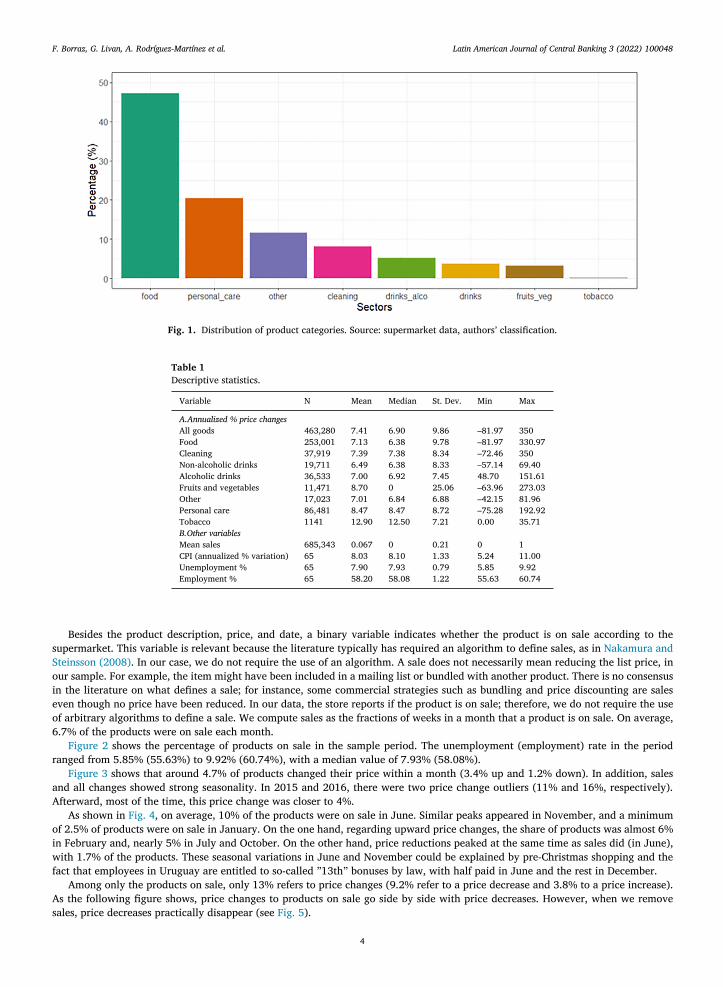
Figure 1 shows the distribution of observations by product category. The food category is the most important, with almost half ofthe sample, followed by personal care. The shares of product categories have not changed much overtime. The only relevant changewas the growing trend in the food and other products categories which comprise about half of the sample.

Table 1 shows summary statistics. The median annualized yearly price change for all the products in the sample was 7.41%, veryclose to the mean inflation of 8.03%. The tobacco category had the highest price increase in the sample. The unemployment ratevaried from a minimum of 5.85 percentage points to a maximum of 9.92 percentage points in the analyzed period.

2 This chain follows a uniform price policy in Montevideo. 3 This category contains heterogeneous products such as shoes, lamps, batteries, newspapers, books, school supplies, pet food, and kitchen items.

3

F. Borraz, G. Livan, A. Rodríguez-Martínez et al. Latin American Journal of Central Banking 3 (2022) 100048

Fig. 1. Distribution of product categories. Source: supermarket data, authors’ classification.

Table 1

Descriptive statistics.

Variable N Mean Median St. Dev. Min Max

A.Annualized % price changes

All goods 463,280 7.41 6.90 9.86 –81.97 350 Food 253,001 7.13 6.38 9.78 –81.97 330.97 Cleaning 37,919 7.39 7.38 8.34 –72.46 350 Non-alcoholic drinks 19,711 6.49 6.38 8.33 –57.14 69.40 Alcoholic drinks 36,533 7.00 6.92 7.45 48.70 151.61 Fruits and vegetables 11,471 8.70 0 25.06 –63.96 273.03 Other 17,023 7.01 6.84 6.88 –42.15 81.96 Personal care 86,481 8.47 8.47 8.72 –75.28 192.92 Tobacco 1141 12.90 12.50 7.21 0.00 35.71 B.Other variables

Mean sales 685,343 0.067 0 0.21 0 1 CPI (annualized % variation) 65 8.03 8.10 1.33 5.24 11.00 Unemployment % 65 7.90 7.93 0.79 5.85 9.92 Employment % 65 58.20 58.08 1.22 55.63 60.74

Besides the product description, price, and date, a binary variable indicates whether the product is on sale according to thesupermarket. This variable is relevant because the literature typically has required an algorithm to define sales, as in Nakamura andSteinsson (2008) . In our case, we do not require the use of an algorithm. A sale does not necessarily mean reducing the list price, inour sample. For example, the item might have been included in a mailing list or bundled with another product. There is no consensusin the literature on what defines a sale; for instance, some commercial strategies such as bundling and price discounting are saleseven though no price have been reduced. In our data, the store reports if the product is on sale; therefore, we do not require the useof arbitrary algorithms to define a sale. We compute sales as the fractions of weeks in a month that a product is on sale. On average,6.7% of the products were on sale each month.

Figure 2 shows the percentage of products on sale in the sample period. The unemployment (employment) rate in the periodranged from 5.85% (55.63%) to 9.92% (60.74%), with a median value of 7.93% (58.08%).

Figure 3 shows that around 4.7% of products changed their price within a month (3.4% up and 1.2% down). In addition, salesand all changes showed strong seasonality. In 2015 and 2016, there were two price change outliers (11% and 16%, respectively).Afterward, most of the time, this price change was closer to 4%.

As shown in Fig. 4 , on average, 10% of the products were on sale in June. Similar peaks appeared in November, and a minimumof 2.5% of products were on sale in January. On the one hand, regarding upward price changes, the share of products was almost 6%in February and, nearly 5% in July and October. On the other hand, price reductions peaked at the same time as sales did (in June),with 1.7% of the products. These seasonal variations in June and November could be explained by pre-Christmas shopping and thefact that employees in Uruguay are entitled to so-called ”13th ” bonuses by law, with half paid in June and the rest in December.

Among only the products on sale, only 13% refers to price changes (9.2% refer to a price decrease and 3.8% to a price increase).As the following figure shows, price changes to products on sale go side by side with price decreases. However, when we removesales, price decreases practically disappear (see Fig. 5 ).

4

F. Borraz, G. Livan, A. Rodríguez-Martínez et al. Latin American Journal of Central Banking 3 (2022) 100048

Fig. 2. Monthly share of products labeled as on sale. Source: supermarket data.

Fig. 3. Monthly share of products whose price changed. Source: supermarket data.

Some products are linked to the official Consumer Price Index (CPI). These products represent 12.1% of the total (14.3% consid-ering only products in 2019).

We consider employment and unemployment data from the Uruguayan National Household Survey (ECH), conducted by the National Institute of Statistics (INE). The ECH is administered throughout the year to generate an accurate picture of the urbanUruguayan employment situation and its socio-economic characteristics. We used data from 2014 to 2019 for Montevideo, the capitalof Uruguay. Fig. 6 shows, from August 2014 to December 2019, the unemployment rate rose, and the employment rate persistentlyfell.

5

F. Borraz, G. Livan, A. Rodríguez-Martínez et al. Latin American Journal of Central Banking 3 (2022) 100048

Fig. 4. Seasonality of the share of products whose price changed. Source: supermarket data.

Fig. 5. Monthly share of products, on sale or not, whose price changed. Source: supermarket data.

There is seasonality in these variables, especially in the unemployment rate (see Fig. 7 ). For example, unemployment grew mostin the last two quarters in the period considered. Therefore, we performed a seasonal adjustment for the empirical analysis. Figs. 8aand 8b analyze each product category’s price dispersion with and without sales. We found no statistically significant differences between the analyses with and without sales except in the “other ” product category, which has a heftier price dispersion with sales.We found other slight differences in the fruits and vegetables and the personal care categories. Dispersion is important to explainconsumer behavior and consumer search costs. For example, according to Stigler (1961) , Carlson and McAfee (1983) , and Janssen andMoraga (2000) , the level of price dispersion is positively related to the number of suppliers.

4. Methodology and results

4.1. Sales and unemployment

We estimated the following fixed-effects panel regression to analyze the relationship between sales and unemployment:

𝑠𝑎𝑙𝑒 𝑖,𝑡 = 𝛼𝑖 + 𝛼𝑡 + 𝛽 ∗ 𝑢𝑛𝑒𝑚𝑝𝑙𝑜𝑦𝑚𝑒𝑛𝑡 𝑡 −3 + 𝜀 𝑖𝑡 (1)

6

F. Borraz, G. Livan, A. Rodríguez-Martínez et al. Latin American Journal of Central Banking 3 (2022) 100048

Fig. 6. Percent change in employment and unemployment rate in Montevideo, Uruguay. Source: Uruguayan National Household Survey (ECH), National Institute of Statistics (INE).

Fig. 7. Mean of percent change in employment and unemployment rate by quarters. Source: Uruguayan National Household Survey (ECH), National Institute of Statistics (INE).

where 𝑠𝑎𝑙𝑒 𝑖,𝑡 is the probability that a product 𝑖 was labeled as on sale by the supermarket in month 𝑡 (we computed sale as the fractionsof weeks in a month that a product was on sale). The right side of the equation features fixed effects for the product ( 𝑖 ) and time ( 𝑡 ),and the unemployment index lagged by three months (because the index is released three months later). Because of the correlationof the error term, we clustered the standard errors at the product and time levels.

Table 2 shows a positive and statistically significant relationship between sales and unemployment (lagged and current). As the economy worsens and unemployment increases, the supermarket uses sales to a greater extent as a mechanism for price adjustment andto stimulate revenue in an adverse scenario. In this way, sales undo the effects of price rigidities in terms of monetary non-neutrality.This increase, although statistically significant, is relatively small. A one-percentage-point increase in the lagged unemployment rate raises the probability of a sale by 0.006 and 0.014 for the case of current unemployment. To quantify this effect, remember

7

F. Borraz, G. Livan, A. Rodríguez-Martínez et al. Latin American Journal of Central Banking 3 (2022) 100048

Fig. 8. Price dispersion with and without sales. Source: Uruguayan National Household Survey (ECH), National Institute of Statistics (INE).

Table 2

Sale probability regression with product- and time-fixed effects.

Dependent variable:

Probability of being on sale

(1) (2)

Unem ploy men 𝑡 𝑡 −3 0.006 ∗∗∗

(0.001) Unemployment 𝑡 0.014 ∗∗∗

(0.001) Observations 685,343 685,343 Adjusted R 2 0.253 0.239

Controls: FE (products and time). Clustered errors at the product and time levels in paren- theses. Note: ∗ p < 0.1; ∗∗ p < 0.05; ∗∗∗ p < 0.01.

that the average probability of sales is 0.067, so a one-percentage-point increase in the unemployment rate raises sales by 11.66%= ((0.067/0.006)-1) ∗ 100.

This result contrasts Coibion et al. (2015) , who found that sales are not relevant from a macroeconomic perspective and notrelated to the business cycle. Moreover, they found that sales are largely acyclical. Our positive and statistically significant effect ofunemployment on sales remained when we used current unemployment instead of three-month lagged unemployment. In this case, the effect double.

As Coibion et al. (2015) point out, the inclusion of time-fixed effects should eliminate endogeneity because of the simultaneousresponse of prices and unemployment to aggregate shocks. Including time-fixed effects allows a causal interpretation of the results. Although our estimates were statistically significant, the economic magnitude of the effect remained relatively low.

In addition to using time- and product-fixed effects, we used instrumental variables with one-period-lagged unemployment as an instrument for current unemployment to avoid endogeneity. Table 3 show this instrumental variable estimation. Our results revealed shows that our instrument was relevant and statistically significant from the first stage. The second stage showed a positive andstatistically significant relationship between unemployment and sales.

In Table 4 , we controlled by the interaction between product and quarter as a robustness check. We found that our instrumentwas still relevant, and there was a positive and statistically significant relationship between sales and unemployment.

We also estimated the same panel regression using price change probability as the dependent variable instead of sale probability.We observed a negative and statistically significant relationship between the probability of price change and unemployment

(lagged and current). This result indicates that price changes become infrequent in the worst stage of the business cycle (see Table 5 ).We also estimated Eq. 1 for each product category in our sample. Table 6 shows that the results remained the same for most

products. Interestingly, we observed a negative and statistically significant relationship between sales and unemployment for the cleaning product category. This result could indicate that cleaning items are procyclical. One possible explanation may be that peoplestay in their homes for longer periods when unemployment rises and are more attentive to cleaning them. Similarly,as it containshome products supplies, the “other ” category behaved in the same way as cleaning products.

8

F. Borraz, G. Livan, A. Rodríguez-Martínez et al. Latin American Journal of Central Banking 3 (2022) 100048

Table 3

Instrumental variables estimates.

Dependent variable:

Probability of being on sale

(1) (2)

Unemployment 𝑡 −3 0.022 ∗∗∗

(0.001) Unemployment 𝑡 0.016 ∗∗∗

(0.001) 1st F-stat 40.94 ∗∗∗ 38.15 ∗∗∗

Observations 685,343 685,343 Adjusted R 2 0.016 0.014

Controls: FE (products and time). Clustered errors at the product and time levels in paren- theses. Note: ∗ p < 0.1; ∗∗ p < 0.05; ∗∗∗ p < 0.01. Instrument: one-period-lagged unemployment.

Table 4

Instrumental variables estimates: Robustness check. Product x quarter fixed effects.

Dependent variable:

Probability of being on sale

(1) (2)

Unemployment 𝑡 −3 0.013 ∗∗∗

(0.0005) Unemployment 𝑡 0.008 ∗∗∗

(0.0005) 1st F-stat 13.67 ∗∗∗ 10.11 ∗∗∗

Observations 685,343 685,343 Adjusted R 2 0.048 0.055

Controls: FE (products interacted with quarter). Clustered errors at the product and quarter levels in parentheses. Note: ∗ p < 0.1; ∗∗ p < 0.05; ∗∗∗ p < 0.01. Instrument: one-period-lagged unemployment.

Table 5

Regression for price change probability with product- and time-fixed effects.

Dependent variable:

Probability of price change

All products Without sales

Unemployment 𝑡 −3 –0.009 ∗∗∗ –0.010 ∗∗∗

(0.0003) (0.0003) Unemployment 𝑡 –0.008 ∗∗∗ –0.011 ∗∗∗

(0.003) (0.004) Observations 685,343 668,624 Adjusted R 2 0.146 0.123

Controls: FE (products and time). Clustered errors at the product and time levels in paren- theses. Note: ∗ p < 0.1; ∗∗ p < 0.05; ∗∗∗ p < 0.01.

Table 6

Regressions for the probability of being on sale by category, with unemployment.

Dependent variable:

Probability of being on sale

Food Pers.care Cleaning Alc. drinks Non-alc. drinks Fruit/veg Other

Unemployment 𝑡 −3 0.008 ∗∗∗ 0.004 ∗∗ –0.006 ∗∗∗ 0.010 ∗∗∗ 0.023 ∗∗∗ 0.009 ∗∗∗ –0.003 ∗∗

(0.001) (0.001) (0.002) (0.002) (0.002) (0.002) (0.002) Obs. 366,936 133,807 55,294 49,059 28,670 18,722 31,243 Adj.R 2 0.232 0.309 0.268 0.197 0.215 0.322 0.414 df = 355,581 128,845 53,274 47,749 27,691 17,886 28,401

Controls: FE (products and time). Clustered errors at the product and time level in parentheses. Note: ∗ p < 0.1; ∗∗ p < 0.05; ∗∗∗ p < 0.01.

9

F. Borraz, G. Livan, A. Rodríguez-Martínez et al. Latin American Journal of Central Banking 3 (2022) 100048

Table 7

Regressions for the probability of being on sale for all and by category with employment.

Dependent variable:

Probability of being on sale

All Food Pers.care Cleaning Alc. drinks Non-alc. drinks Fruit/veg Other

Employment 𝑡 −3 –0.004 ∗∗∗ –0.006 ∗∗∗ –0.003 ∗∗ 0.004 ∗∗∗ –0.007 ∗∗∗ –0.016 ∗∗∗ –0.006 ∗∗∗ –0.002 (0.001) (0.0005) (0.001) (0.001) (0.001) (0.002) (0.002) (0.001)

Obs. 685,343 366,936 133,807 55,294 49,059 28,670 18,722 31,243 Adj.R 2 0.253 0.232 0.309 0.268 0.197 0.215 0.322 0.414 df = 661,377 355,581 128,845 53,274 47,749 27,691 17,886 28,401

Controls: FE (products and time). Clustered errors at the product and time levels in parentheses. Note: ∗ p < 0.1; ∗∗ p < 0.05; ∗∗∗ p < 0.01.

Table 8

Regressions for the probability of count sale and count price change with unemployment.

Dependent variable:

Number of weeks on sale in the month Number of price changes in the month

All products All products Without sales

Unemployment 𝑡 −3 0.040 ∗∗∗ –0.011 ∗∗∗ –0.012 ∗∗∗

(0.002) (0.001) (0.001) Observations 685,343 685,343 668,624 Adjusted R 2 0.230 0.141 0.116

Controls: FE (products and time). Clustered errors at the product and time levels in parentheses. Note: ∗ p < 0.1; ∗∗ p < 0.05; ∗∗∗ p < 0.01.

Table 9

Regression for the sale probability with product- and time-fixed effects Sample of products in stock in more than half of the periods.

Dependent variable:

Probability of being on sale Probability of price change

All products All products Without sales

Unemployment 𝑡 −3 0.008 ∗∗∗ –0.0094 ∗∗∗ –0.0113 ∗∗∗

(0.001) (0.00025) (0.00027) Observations 529,085 529,085 514,216 Adjusted R 2 0.223 0.1505 0.1208

Controls: FE (products and time). Clustered errors at the product and time levesl in parentheses. Note: ∗ p < 0.1; ∗∗ p < 0.05; ∗∗∗ p < 0.01.

One concern with the previous results is that individuals can shift from being employed to being out of the labor force (inactive)during a recession. For this reason, the unemployment rate alone is not a good measure of economic conditions. Therefore, asa robustness check, we estimated the sales regression against the employment rate (defined as the number of employed peopledivided by the total labor force). Table 7 shows the results of using seasonally adjusted employment data with three lags insteadof unemployment alone. Contrary to our previous analysis, the “other ” category yielded a statistically non-significant relationship between sales and employment. This could be explained by the heterogeneity of this category’s products (residual category).

As an additional robustness check, we replaced the probability of sale with the number of weeks the product was on sale as adependent variable. Table 8 shows the relationship between lagged unemployment and the number of weeks each product type wason sale. Our previous results held as we noted a positive and statistically significant relationship between unemployment and sales.Regarding the relationship between lagged unemployment and the number of price changes in a month, we again observed a negativeand statistically significant relationship when considering all products without sales.

Because not all products are available all the time, we estimated Eq. 1 for the subsample of 9626 products in stock in more thanhalf of the periods as a final robustness check. The results in Table 9 are similar to our previous findings.

4.2. Correlation and Granger causality analysis

In this section, we describe the price correlation structure of the products introduced above. Given their partition in terms ofsectors (e.g., food, drinks), such products are naturally organized in clusters. We reasonably expected correlations between prices tobe stronger among products belonging to the same clusters. This structure naturally lends itself to dimensionality reduction, which we performed using PCA. In a nutshell, extracted time series data (the principal components) from each sector. Their dynamics over

10

F. Borraz, G. Livan, A. Rodríguez-Martínez et al. Latin American Journal of Central Banking 3 (2022) 100048

Table 10

Summary statistics of the first two PCs of each sector. 𝑛 + denotes the fraction of positive components in the corresponding eigenvectors.

1st PC 2nd PC

𝑛 + % of var. explained 𝑛 + % of var. explained

Food 72.3% 45.6% 56.4% 11.6%

Pers. care 68.8% 43.2% 50.8% 11.7%

Cleaning 70.3% 43.9% 55.2% 10.3%

Alc. drinks 68.1% 55.0% 55.2% 10.5%

Drinks 68.1% 39.1% 53.8% 12.1%

Fruits and veg. 75.5% 31.2% 55.1% 12.1%

Other 60.2% 34.4% 68.1% 16.1%

Table 11

Pearson correlation between employment and unemployment rates and the value of the first PC of each sector in the final week of the month of the indicators’ publication.

Employment Unemployment

Food 0.920 ∗∗∗ -0.796 ∗∗∗

Pers. care 0.917 ∗∗∗ -0.807 ∗∗∗

Cleaning 0.922 ∗∗∗ -0.804 ∗∗∗

Alc. drinks 0.907 ∗∗∗ -0.768 ∗∗∗

Drinks 0.913 ∗∗∗ -0.797 ∗∗∗

Fruits and veg. 0.882 ∗∗∗ -0.747 ∗∗∗

Other 0.901 ∗∗∗ -0.802 ∗∗∗

Note: ∗ p < 0.1; ∗∗ p < 0.05; ∗∗∗ p < 0.01.

time represent the price dynamics of all or some of a sector’s products. Then, we tested whether such time series displayed statisticallysignificant correlations or causal relationships with our macroeconomic variables of interest.

To the best of our knowledge, this approach to price rigidity analysis is entirely novel. PCA is a widely used tool to explain thevariance of multivariate datasets through interpretable synthetic variables (principal components) that can be ranked in terms of relative importance. However, PCA is not frequently used in the time domain, which is key to our analysis. We compressed eachsector’s product price dynamics over hundreds or thousands of time series into just two time series, which in all cases accounted formore than half of each sector’s price variance. Appendix Appendix A provides a short overview of PCA in the temporal domain, whichwe extensively leveraged.

The first two columns of Table 10 show summary statistics for all sectors’ first principal components (PCs) in the price-time series.We report the fraction 𝑛 + of positive components in the first two eigenvectors of each sector’s correlation matrix (as explained inAppendix Appendix A , quantifies the fraction of variables that share a positive correlation with the corresponding PC) and the fractionof variance explained by the corresponding PC. As seen from the latter number, the first PC of each sector explained a considerablylarge proportion of the variance of its price dynamics, ranging from more than 30% to 55% in the case of alcoholic drinks. Furthermore,the 𝑛 + values– all abundantly greater than 50% – showed that the first PC was a clear source of positive correlation among most productprices in each sector.

Our results showed that more than half of the variance in price dynamics for each sector can be explained by the first two PCs,suggesting that such quantities may hold relevant information concerning our macroeconomic variables of interest. Table 11 depicts the correlation between monthly employment status and the values of each sector’s first PC in the final week of the same month. Weobserved a remarkably strong positive (negative) correlation between employment (unemployment) and the first PCs ( 𝑝 < . 01 in allcases). Correlations with second PCs were not statistically significant ( 𝑝 > 0 . 1 in all cases) and are therefore not reported. The positivecorrelation among all sector’s first PCs and employment is visually clear from Fig. 9 , in which we plotted all standardize variables’time evolution.

The above results clearly hint at a rather strong relationship between employment / unemployment status and the price dynamicsof the sectors we considered, as explained by the first PC. We further investigated this by measuring causal interactions in the Grangersense. In Table 12 we report the results of Granger causality tests, which determine whether variation in one variable is explanatoryof future variation in another variable with a certain time lag (for a complete description of the test, see Granger (1969) ). Here,we tested whether employment / unemployment Granger-caused each sector’s first two PCs in the final week of the second monthafter their values were published. We find substantial Granger causality across the board. In particular, we found that employmentGranger-caused the first two PCs of all sectors except for “other ” with different levels of statistical significance In addition, we foundthat unemployment Granger-caused the first PCs in the alcoholic drinks and fruits and vegetables sectors, and the second PCs of allsectors except for food, and other. We also find robust evidence of reverse causal relationships by testing whether the first two PCs ofeach sector in the final week of each month Granger-cause employment / unemployment in the following month (see Table 13 ). Wefind that the first PCs of each sector Granger-caused both indicators except unemployment in the case of the ‘other’ sector. Conversely,

11

F. Borraz, G. Livan, A. Rodríguez-Martínez et al. Latin American Journal of Central Banking 3 (2022) 100048

Fig. 9. Time evolution of the PCs of the seven product sectors (grey solid lines) and employment (purple dots and dashed line). Employment time series standardized for comparison. (For interpretation of the references to colour in this figure legend, the reader is referred to the web version of this article.).

Table 12

F-statistics of Granger causality tests between employment and unemployment rates and first and second PCS in the final week of the second month after indicators publications.

1st PC 2nd PC

Employment Unemployment Employment Unemployment

Food 5.07 ∗∗∗ 2.19 5.57 ∗∗ 2.48 Pers. care 6.46 ∗∗ 2.71 5.27 ∗∗ 6.91 ∗∗∗

Cleaning 5.92 ∗∗∗ 1.45 6.98 ∗∗ 5.08 ∗∗∗

Alc. drinks 6.47 ∗∗ 8.07 ∗∗∗ 1.80 ∗∗∗ 1.50 ∗∗∗

Drinks 3.81 ∗∗ 9.86 1.59 ∗∗∗ 7.32 ∗∗∗

Fruits and veg. 1.75 ∗∗∗ 1.80 ∗∗∗ 1.79 ∗∗∗ 8.15 ∗∗∗

Other 0.16 8.69 2.52 1.67

Note: ∗ p < 0.1; ∗∗ p < 0.05; ∗∗∗ p < 0.01.

Table 13

F-statistics of reverse Granger causality tests between employment and unemployment rates and first and second PCs in the final week of the month prior to publication of the indicators.

1st PC 2nd PC

Employment Unemployment Employment Unemployment

Food 23.7 ∗∗∗ 10.6 ∗∗∗ 4.17 2.67 Pers. care 20.1 ∗∗∗ 11.7 ∗∗∗ 0.14 0.88 Cleaning 26.3 ∗∗∗ 11.4 ∗∗∗ 2.11 0.87 Alc. drinks 10.7 ∗∗∗ 8.11 ∗∗∗ 0.31 1.02 Drinks 22.0 ∗∗∗ 9.97 ∗∗∗ 0.14 0.87 Fruits and veg. 13.2 ∗∗∗ 6.08 0.20 1.10 Other 10.4 ∗∗∗ 9.66 ∗∗∗ 6.98 ∗∗∗ 6.77 ∗∗∗

Note: ∗ p < 0.1; ∗∗ p < 0.05; ∗∗∗ p < 0.01.

the ‘other’ sector was the only one for which we detected a statistically significant causal relationship between the second PC andboth employment and unemployment in the following month.

Appendix Appendix B (see Tables B.14 and B.15 ) shows the results obtained when testing for direct and reverse Granger causalitywith four additional weeks of time lag. We found that the Granger causality from both employment and unemployment to the firstPC faded away almost without exception, whereas it remained fairly strong with respect to most sectors’ second PCs. Conversely, wefound that each sector’s PCs still Granger-caused the indicators, and the relationship remains statistically significant even for greater time lags (see Tables B.14 and B.15 ). Similar results are obtained when testing for Granger and reverse Granger causality betweenemployment status and the average weekly values of the first and second PCs computer over months before and after indicators’publication (see Tables B.16 and B.17 ).

12

F. Borraz, G. Livan, A. Rodríguez-Martínez et al. Latin American Journal of Central Banking 3 (2022) 100048

5. Conclusions

We used a rich weekly price database from the largest supermarket chain in Uruguay to analyze the relationships among prices,sales, and business cycle conditions captured by the unemployment / employment rate. Our results showed a statistically significantbut small positive relationship between unemployment and prodcut categories’ price dynamics. In this way, sales undo part of theeffects of price rigidities in terms of monetary non-neutrality. As this effect is relatively small, sales do not alleviate rigidities in aneconomic recession.

Regarding product categories, food products, alcoholic drinks, non-alcoholic drinks, and fruits and vegetables displayed strong and positive statistically significant relationships between the probability of being on sale and unemployment rates. On the other hand, food products, cleaning, alcoholic drinks, non-alcoholic drinks, and fruits and vegetables all displayed and negative statistically significant relationships between the probability of being on sale and employment rates.

We also performed a novel time-series PCA and found that all product categories shared a mutual correlation structure. Themost statistically significant correlation occurred between employment variation and the first principal component for each product category. We also observed substantial Granger causality between unemployment rates and the first principal component of the alcoholic drinks and fruits and vegetable sectors.

Declaration of Competing Interest

There is no conflict of interest.

Appendix A. Principal component analysis

This section provides a quick overview of PCA in the time domain, which we used extensively in our correlation and Grangercausality analyses. Suppose we are interested in studying the statistical properties of 𝑁 time series, each one made of 𝑇 observations.Let us collect their standardized data (i.e., zero mean and unit variance) 𝑥 𝑖𝑡 – with 𝑖 = 1 , … , 𝑁 , and 𝑡 = 1 , … , 𝑇 – in an 𝑁 × 𝑇 matrix𝐗 , which we can then use to construct the 𝑁 ×𝑁 Pearson correlation matrix 𝐂 = 𝐗𝐗

T ∕ 𝑇 . By definition, such a matrix is symmetricand positive definite. Hence, it yields 𝑁 non-negative eigenvalues 𝜆1 ≥ 𝜆2 ≥ … ≥ 𝜆𝑁

≥ 0 . The corresponding eigenvalue problem canbe written as

𝐂𝐕

( 𝑖 ) = 𝜆𝑖 𝐕

( 𝑖 ) (2)

where 𝐕

( 𝑖 ) = ( 𝑉 ( 𝑖 ) 1 , 𝑉 ( 𝑖 ) 2 , … , 𝑉

( 𝑖 ) 𝑁

) is the normalized eigenvector for the 𝑖 -th eigenvalue. Since 𝐂 is symmetric, the eigenvectors 𝐕

( 𝑖 ) are

mutually orthogonal (i.e., ∑𝑁

𝑗=1 𝑉 ( 𝑖 ) 𝑗

𝑉 ( 𝓁) 𝑗

= 0 for 𝑖 ≠ 𝓁). The main point about PCA is that the set of 𝑁 time series 𝑥 𝑖𝑡 can be mapped onto a set of 𝑁 exactly uncorrelated standardized time

series 𝑒 𝑖𝑡 , called principal components (PCs). This is achieved with the following linear transformation:

𝑒 𝑖𝑡 =

1 √𝜆𝑖

𝑁 ∑

𝑗=1 𝑉

( 𝑖 ) 𝑗

𝑥 𝑗𝑡 , (3)

where

𝑥 𝑖𝑡 =

𝑁 ∑

𝑘 =1

√𝜆𝑘 𝑉

( 𝑘 ) 𝑖

𝑒 𝑘𝑡 . (4)

By exploiting eigenvector orthogonality one can immediately verify that the new variables introduced in Eq. (4) are indeed uncor-related:

1 𝑇

𝑇 ∑

𝑡 =1 𝑒 𝑖𝑡 𝑒 𝑗𝑡 = 𝛿𝑖𝑗 , (5)

where 𝛿𝑖𝑗 = 1 if 𝑖 = 𝑗 and 𝛿𝑖𝑗 = 0 otherwise. All in all, Eq. (4) shows that the result of the PCA mapping is to decompose the time evolution of each time series 𝑥 𝑖 into 𝑁

uncorrelated contributions whose standard deviation is proportional to the square root of the eigenvalues of the empirical correlationmatrix. Therefore, the ratios 𝜆𝑖 ∕ 𝑁 quantify the fraction of the overall variance in the original data explained by the 𝑖 -th PC.

Now, suppose that a few eigenvalues (e.g., the first 𝑀) are much greater than the remaining ones. Then, by virtue of Equation (4) ,one could approximate each 𝑥 𝑖 as

𝑥 𝑖𝑡 ∼𝑀 ∑

𝑘 =1

√𝜆𝑘 𝑉

( 𝑘 ) 𝑖

𝑒 𝑘𝑡 . (6)

In the limiting case of a single eigenvalue being much larger than any other ( 𝜆1 ≫ 𝜆𝑖 for 𝑖 = 2 , … , 𝑁) one could eventually approximateall variables using the first PC 𝑒 1 :

𝑥 𝑖𝑡 ∼√𝜆1 𝑉

(1) 𝑖

𝑒 1 𝑡 . (7)

13

F. Borraz, G. Livan, A. Rodríguez-Martínez et al. Latin American Journal of Central Banking 3 (2022) 100048

Despite being rather crude, the above approximation is a useful first step to understanding multivariate time series’ collective dynamics. In particular, inspecting the first eigenvector’s components ( 𝑉 (1) 1 , … , 𝑉

(1) 𝑁

) provides relevant insight into the role played by

the first PC. In fact, when most components 𝑉 (1) 𝑖

share the same sign, the first PC 𝑒 1 acquires a clear meaning as a source of positivecorrelation in the system, as it “drives ” most variables 𝑥 𝑖 in the same direction.

If we extend the simple approximation in Eq. (7) to include the second PC, we obtain

𝑥 𝑖𝑡 ∼√𝜆1 𝑉

(1) 𝑖

𝑒 1 𝑡 +

√𝜆2 𝑉

(2) 𝑖

𝑒 2 𝑡 . (8)

Analogous to the above consideration, inspecting the second eigenvector’s components ( 𝑉 (2) 1 , … , 𝑉 (2) 𝑁

) determines the interpretationof the second PC as a source of additional correlation with respect to the correlations encoded in the first PC. Similar considerationsapply to all following PCs.

Appendix B

Additional tables on Granger causality

Table B1

F-statistics of Granger causality tests between employment and unemployment rates and first and second PCs values in the final week of the third month after the indicators’ publi- cation.

1st PC 2nd PC

Employment Unemployment Employment Unemployment

Food 3.74 0.31 9.95 ∗∗∗ 5.71 ∗∗∗

Pers. care 2.46 0.91 16.3 ∗∗∗ 10.5 ∗∗∗

Cleaning 3.75 0.25 12.2 ∗∗∗ 4.35 Alc. drinks 3.35 0.14 21.6 ∗∗∗ 13.1 ∗∗∗

Drinks 5.13 ∗∗∗ 1.73 20.3 ∗∗∗ 6.03 ∗∗∗

Fruits and veg. 3.82 0.97 6.59 ∗∗∗ 4.37 Other 3.62 0.68 1.74 0.75

Note: ∗ p < 0.1; ∗∗ p < 0.05; ∗∗∗ p < 0.01.

Table B2

F-statistics of reverse Granger causality tests between employment and unemployment rates and first and second PCs in the final week of the second month before the indicators’ pub- lication .

1st PC 2nd PC

Employment Unemployment Employment Unemployment

Food 21.2 ∗∗∗ 8.04 ∗∗∗ 3.19 5.45 ∗∗∗

Pers. care 11.9 ∗∗∗ 7.93 ∗∗∗ 2.47 4.61 Cleaning 23.8 ∗∗∗ 8.14 ∗∗∗ 8.58 ∗∗ 5.02 ∗∗∗

Alc. drinks 16.1 ∗∗∗ 7.33 ∗∗∗ 0.66 5.49 ∗∗∗

Drinks 10.9 ∗∗∗ 7.74 ∗∗∗ 5.37 ∗∗ 5.62 ∗∗∗

Fruits and veg. 11.8 ∗∗∗ 6.02 ∗∗∗ 0.60 3.61 Other 15.5 ∗∗∗ 10.0 ∗∗∗ 1.57 4.65

Note: ∗ p < 0.1; ∗∗ p < 0.05; ∗∗∗ p < 0.01.

14

F. Borraz, G. Livan, A. Rodríguez-Martínez et al. Latin American Journal of Central Banking 3 (2022) 100048

Table B3

F-statistics of Granger causality tests between average weekly values of the first and second PCs in a month and the following month’s employment and unemployment .

1st PC 2nd PC

Employment Unemployment Employment Unemployment

Food 2.67 1.21 3.51 1.46 Pers. care 3.94 1.67 8.93 ∗∗∗ 10.7 ∗∗∗

Cleaning 4.75 1.22 9.22 ∗∗∗ 3.52 Alc. drinks 2.47 2.27 6.46 ∗∗∗ 7.36 ∗∗∗

Drinks 3.72 0.19 9.77 ∗∗∗ 7.07 Fruits and veg. 2.99 1.05 4.09 1.71 Other 5.68 1.37 16.2 ∗∗∗ 9.19 ∗∗∗

Note: ∗ p < 0.1; ∗∗ p < 0.05; ∗∗∗ p < 0.01.

Table B4

F-statistics of Granger causality tests between employment and unemployment rates and the following month’s average weekly values of the first and second PCs .

1st PC 2nd PC

Employment Unemployment Employment Unemployment

Food 20.2 ∗∗∗ 11.3 ∗∗∗ 3.07 0.88 Pers. care 27.3 ∗∗∗ 13.1 ∗∗∗ 0.19 0.84 Cleaning 31.7 ∗∗∗ 12.0 ∗∗∗ 0.15 0.82 Alc. drinks 20.1 ∗∗∗ 8,33 ∗∗∗ 3.25 1.02 Drinks 26.0 ∗∗∗ 8.61 ∗∗∗ 0.14 0.84 Fruits and veg. 13.7 ∗∗∗ 7.33 ∗∗∗ 2.55 2.76 Other 24.6 ∗∗∗ 10.7 ∗∗∗ 1.21 3.05

Note: ∗ p < 0.1; ∗∗ p < 0.05; ∗∗∗ p < 0.01.

References

Anderson, E., Malin, B.A., Nakamura, E., Simester, D., Steinsson, J., 2017. Informational rigidities and the stickiness of temporary sales. J Monet Econ 90 (C), 64–83 .Bils, M., Klenow, P.J., 2004. Some evidence on the importance of sticky prices. Journal of Political Economy 112 (5), 947–985. doi: 10.1086/422559 . Blinder, A., 1991. Why are prices sticky? preliminary results from an interview study. American Economic Review 81 (2), 89–96 . Calvo, G.A., 1983. Staggered prices in a utility-maximizing framework. J Monet Econ 12 (3), 383–398 . Carlson, J.A., McAfee, R.P., 1983. Discrete equilibrium price dispersion. Journal of Political Economy 91 (3), 480–493 . Coibion, O., Gorodnichenko, Y., Hong, G.H., 2015. The cyclicality of sales, regular and effective prices: business cycle and policy implications. American Economic

Review 105 (3), 993–1029 . Eichenbaum, M., Jaimovich, N., Rebelo, S., 2011. Reference prices, costs, and nominal rigidities. American Economic Review 101 (1), 234–262 . Gagnon, E., López-Salido, D., Sockin, J., 2017. The cyclicality of sales, regular, and effective prices: business cycle and policy implications: comment. American

Economic Review 107 (10), 3229–3242 . Galí, J., 2008. Monetary Policy, Inflation, and the Business Cycle: An Introduction to the New Keynesian Framework. Princeton University Press . Glandon, P.J., 2018. Sales and the (mis) measurement of price level fluctuations. J Macroecon 58, 60–77 . Golosov, M., Lucas Jr, R.E., 2007. Menu costs and phillips curves. Journal of Political Economy 115 (2), 171–199 . Granger, C.W.J., 1969. Investigating causal relations by econometric models and cross-spectral methods. Econometrica 37 (3), 424–438 . Janssen, M.C., Moraga, J.L., 2000. Pricing, Consumer Search and the Size of Internet Markets. Tinbergen Institute Discussion Papers. Tinbergen Institute . Kehoe, P., Midrigan, V., 2015. Prices are sticky after all. J Monet Econ 75, 35–53 . Klenow, P.J., Kryvtsov, O., 2008. State-dependent or time-dependent pricing: does it matter for recent u.s. inflation? Q J Econ 123 (3), 863–904 . Klenow, P.J., Malin, B.A., 2010. Microeconomic evidence on price-setting. In: Friedman, B.M., Woodford, M. (Eds.), Handbook of Monetary Economics. In: Handbook

of Monetary Economics, Vol. 3. Elsevier, pp. 231–284 . Kryvtsov, O., Vicent, N., 2021. The cyclicality of sales and aggregate price flexibility. Review of Economic Studies 88 (1), 334–377 . Lucas, R.J., 1972. Expectations and the neutrality of money. J Econ Theory 4 (2), 103–124 . Mankiw, G.R.R., 2002. Sticky information versus sticky prices: a proposal to replace the new keynesian phillips curve. Q J Econ 117 (4), 1293–1328 . MEF, 2020. Informe circN ◦42-20: Asunto N ◦ 23/2020: Flater S.R.L. (Tienda Inglesa) y otros - Almacenes Éxito S.A. y otros. Technical Report. Ministry of Economy

and Finance, Uruguay . Nakamura, E., Steinsson, J., 2008. Five facts about prices: a reevaluation of menu cost models. Q J Econ 123 (4), 1415–1464 . Nakamura, E., Steinsson, J., 2013. Price rigidity: microeconomic evidence and macroeconomic implications. Annu. Rev. Econ. 5 (1), 133–163 . Sims, C.A., 2003. Implications of rational inattention. J Monet Econ 50 (3), 665–690 . Stigler, G.J., 1961. The economics of information. Journal of Political Economy 69 (3), 213–225 . Taylor, J.B., 1979. Staggered wage setting in a macro model. Am Econ Rev 69 (2), 108–113 . Taylor, J.B., 1980. Aggregate dynamics and staggered contracts. Journal of Political Economy 88 (1), 1–23 .

15