Lecture Notes1 ECON 323 Microeconomic Theory
281
Lecture Notes 1 ECON 323 Microeconomic Theory Guoqiang TIAN Department of Economics Texas A&M University College Station, Texas 77843 ([email protected]) This version: April, 2022 1 This lecture notes are for the purpose of my teaching and convenience of my students in class.
-
Upload
khangminh22 -
Category
Documents
-
view
1 -
download
0
Transcript of Lecture Notes1 ECON 323 Microeconomic Theory

Lecture Notes1
ECON 323
Microeconomic Theory
Guoqiang TIAN
Department of Economics
Texas A&M University
College Station, Texas 77843
This version: April, 2022
1This lecture notes are for the purpose of my teaching and convenience of my studentsin class.

ii

Contents
I Preliminaries and the Basics of Demand and Supply 1
1 Economics Review and Math Review 5
1.1 Economics Review . . . . . . . . . . . . . . . . . . . . . . . . 5
1.1.1 The Themes of Economics . . . . . . . . . . . . . . . . 5
1.1.2 The Themes of Microeconomics . . . . . . . . . . . . 9
1.1.3 Positive versus Normative Analysis . . . . . . . . . . 11
1.1.4 What is a Market? . . . . . . . . . . . . . . . . . . . . 11
1.1.5 Real versus Nominal Prices . . . . . . . . . . . . . . . 12
1.1.6 Production possibility frontier (PPF) . . . . . . . . . . 16
1.1.7 Why study microeconomics? . . . . . . . . . . . . . . 16
1.2 Math Review . . . . . . . . . . . . . . . . . . . . . . . . . . . . 17
1.2.1 Equations for straight lines . . . . . . . . . . . . . . . 18
1.2.2 Solve two equations with two unknowns . . . . . . . 19
1.2.3 Derivatives . . . . . . . . . . . . . . . . . . . . . . . . 21
1.2.4 Functions of multiple variables . . . . . . . . . . . . . 23
2 Market Analysis 25
2.1 Demand . . . . . . . . . . . . . . . . . . . . . . . . . . . . . . 25
2.2 Supply . . . . . . . . . . . . . . . . . . . . . . . . . . . . . . . 33
2.3 Determination of Equilibrium Price and Quantity . . . . . . 36
2.4 Market Adjustment . . . . . . . . . . . . . . . . . . . . . . . . 39
2.5 Elasticity of Demand and Supply . . . . . . . . . . . . . . . . 44
2.5.1 Elasticity of Demand . . . . . . . . . . . . . . . . . . . 45
iii

iv CONTENTS
2.5.2 Elasticity and Total Expenditure . . . . . . . . . . . . 49
2.5.3 Price Elasticity of Supply . . . . . . . . . . . . . . . . 51
2.5.4 Short-Run versus Long-Run Elasticities . . . . . . . . 53
2.6 Effects on Government Intervention: Price Controls . . . . . 55
II Demand Side of Market 59
3 Theory of Consumer Choice 63
3.1 Budget Constraints . . . . . . . . . . . . . . . . . . . . . . . . 63
3.1.1 Budget Line . . . . . . . . . . . . . . . . . . . . . . . . 63
3.1.2 Changes in Budget Line . . . . . . . . . . . . . . . . . 65
3.2 Consumer Preferences . . . . . . . . . . . . . . . . . . . . . . 67
3.2.1 Basic Assumptions on Preferences . . . . . . . . . . . 67
3.2.2 Properties of Indifference Curves . . . . . . . . . . . . 69
3.2.3 Marginal Rate of Substitution . . . . . . . . . . . . . . 70
3.2.4 Special Shapes of Indifference Curves: . . . . . . . . . 72
3.2.5 Utility Functions . . . . . . . . . . . . . . . . . . . . . 75
3.3 Consumer’s Optimal Choice . . . . . . . . . . . . . . . . . . . 79
3.4 The Composite-Good Convention . . . . . . . . . . . . . . . 84
3.5 Revealed Preference . . . . . . . . . . . . . . . . . . . . . . . 85
4 Individual and Market Demand 87
4.1 Effect of Income Change . . . . . . . . . . . . . . . . . . . . . 87
4.2 Derivation of the Demand Curve from Utility Maximization 92
4.3 Income and Substitution Effects of a Price Change . . . . . . 95
4.4 From Individual to Market Demand . . . . . . . . . . . . . . 101
4.5 Consumer Surplus . . . . . . . . . . . . . . . . . . . . . . . . 102
4.6 Network Externalities . . . . . . . . . . . . . . . . . . . . . . 105

CONTENTS v
III Supply Side of Market 109
6 Theory of Production 113
6.1 The Technology of Production . . . . . . . . . . . . . . . . . . 113
6.2 Production in Short-Run . . . . . . . . . . . . . . . . . . . . . 115
6.2.1 Various Product Curves in Short Run . . . . . . . . . 115
6.2.2 The Geometry of Production Curves . . . . . . . . . . 118
6.2.3 The Law of Diminishing Marginal Returns . . . . . . 119
6.2.4 Labor Productivity and the Standard of Living . . . . 121
6.3 Production in the Long-Run . . . . . . . . . . . . . . . . . . . 122
6.3.1 Production Isoquants . . . . . . . . . . . . . . . . . . . 122
6.3.2 Marginal Rate of Technical Substitution . . . . . . . . 123
6.3.3 Returns to Scale . . . . . . . . . . . . . . . . . . . . . . 125
7 The Cost of Production 129
7.1 The Nature of Cost . . . . . . . . . . . . . . . . . . . . . . . . 129
7.2 Short-Run Costs of Production . . . . . . . . . . . . . . . . . 130
7.2.1 Short-Run Total, Average, and Marginal Costs . . . . 130
7.2.2 The Shapes of Short-Run Cost Curves . . . . . . . . . 134
7.3 Long-Run Costs of Production . . . . . . . . . . . . . . . . . 137
7.3.1 Isocost Line . . . . . . . . . . . . . . . . . . . . . . . . 138
7.3.2 Cost Minimization Problem . . . . . . . . . . . . . . . 139
7.3.3 Long-Run Cost Curves . . . . . . . . . . . . . . . . . . 142
7.3.4 Input Price Changes and Cost Curves . . . . . . . . . 145
7.3.5 Economies of Scale and Diseconomies of Scale . . . . 145
7.4 Short-Run Verses Long-Run Average Cost Curves . . . . . . 146
7.5 Economies and Diseconomies of Scope . . . . . . . . . . . . . 148
7.6 Using Cost Curves: Controlling Pollution . . . . . . . . . . . 149
8 Profit Maximization and Competitive Firm 151
8.1 Demand Curve under Competition . . . . . . . . . . . . . . . 151
8.2 Short-Run Profit Maximization . . . . . . . . . . . . . . . . . 153

vi CONTENTS
8.3 Competitive Firm’s Short-run Supply Curve . . . . . . . . . 161
8.4 Output Response to a Change in Input Prices . . . . . . . . . 161
8.5 Producer Surplus in the Short Run . . . . . . . . . . . . . . . 162
8.6 Long-Run Profit Maximization . . . . . . . . . . . . . . . . . 164
9 Competitive Markets 165
9.1 The Short-Run Industry Supply Curve . . . . . . . . . . . . . 166
9.2 Long-Run Competitive Equilibrium . . . . . . . . . . . . . . 167
9.3 The Long-Run (LR) Supply Curve . . . . . . . . . . . . . . . 170
9.4 Gains and Losses from Government Policies . . . . . . . . . 173
9.4.1 Consumer and Producer Surplus . . . . . . . . . . . . 173
9.4.2 The Efficiency of Competitive Markets . . . . . . . . 176
9.5 Minimum Prices (Price Floor) . . . . . . . . . . . . . . . . . . 177
IV Market Structure and Competitive Strategy 181
10 Monopoly and Monopsony 185
10.1 The Nature of Monopoly . . . . . . . . . . . . . . . . . . . . . 185
10.2 Sources of Monopoly Power . . . . . . . . . . . . . . . . . . . 186
10.3 The Monopoly’s Demand and Marginal Revenue Curves . . 188
10.4 Monopolist’s Decision . . . . . . . . . . . . . . . . . . . . . . 190
10.4.1 Monopolist’s Profit Maximization . . . . . . . . . . . 190
10.4.2 The Multiplant Firm . . . . . . . . . . . . . . . . . . . 194
10.4.3 Relationships between MR, Price, and EPd . . . . . . . 195
10.4.4 A Rule of Thumb for Pricing . . . . . . . . . . . . . . 198
10.4.5 Measuring Monopoly Power . . . . . . . . . . . . . . 199
10.5 Further Implications of Monopoly Analysis . . . . . . . . . . 200
10.6 Monopoly versus Perfect Competition . . . . . . . . . . . . . 201
10.7 The Social Cost of Monopoly Power . . . . . . . . . . . . . . 202
10.7.1 Income Distribution Problem . . . . . . . . . . . . . . 202
10.7.2 Inefficient Allocations . . . . . . . . . . . . . . . . . . 203
10.8 Benefits of Monopoly: Corporate Innovation . . . . . . . . . 204

CONTENTS vii
10.9 Monopsony . . . . . . . . . . . . . . . . . . . . . . . . . . . . 205
10.9.1 Competitive Buyer Compared to Competitive Seller . 206
10.9.2 Monopsony Buyer . . . . . . . . . . . . . . . . . . . . 206
10.10Monopsony Power . . . . . . . . . . . . . . . . . . . . . . . . 208
10.10.1 Monopsony Power: Elastic versus Inelastic Supply . 208
10.10.2 Sources of Monopsony Power . . . . . . . . . . . . . . 208
10.10.3 The Social Costs of Monopsony Power . . . . . . . . 209
10.10.4 Bilateral Monopsony . . . . . . . . . . . . . . . . . . . 210
10.11Limiting Market Power: The Antitrust Laws . . . . . . . . . 210
11 Pricing with Market Power 213
11.1 Capturing Consumer Surplus . . . . . . . . . . . . . . . . . . 213
11.2 First-Degree Price Discrimination . . . . . . . . . . . . . . . . 214
11.2.1 Capturing Consumer Surplus by Perfect Price Dis-
crimination . . . . . . . . . . . . . . . . . . . . . . . . 214
11.2.2 Capturing Consumer Surplus by Imperfect Price Dis-
crimination . . . . . . . . . . . . . . . . . . . . . . . . 215
11.3 Second-Degree Price Discrimination . . . . . . . . . . . . . . 216
11.4 Third-Degree Price Discrimination . . . . . . . . . . . . . . . 216
11.5 The Two-Part Tariff . . . . . . . . . . . . . . . . . . . . . . . . 219
11.5.1 Two-Part Tariff with a Single Consumer . . . . . . . . 219
11.5.2 Two-Part Tariff with Two Consumer . . . . . . . . . . 220
11.6 Intertemporal Price Discrimination and Peak-Load Pricing . 222
11.7 Bundling . . . . . . . . . . . . . . . . . . . . . . . . . . . . . . 223
12 Monopolistic Competition and Oligopoly 225
12.1 Monopolistic Competition . . . . . . . . . . . . . . . . . . . . 226
12.1.1 Short-Run Equilibrium . . . . . . . . . . . . . . . . . . 226
12.1.2 Long-Run Equilibrium . . . . . . . . . . . . . . . . . . 227
12.1.3 Monopolistic Competition and Economic Efficiency . 228
12.2 Oligopoly . . . . . . . . . . . . . . . . . . . . . . . . . . . . . 229
12.3 Quantity Competition . . . . . . . . . . . . . . . . . . . . . . 234

viii CONTENTS
12.3.1 Cournot Model . . . . . . . . . . . . . . . . . . . . . . 234
12.3.2 The Stackelberg Model—First Mover Advantage . . . 239
12.4 Price Competition . . . . . . . . . . . . . . . . . . . . . . . . . 240
12.4.1 Price Competition with Homogeneous Products—
The Bertrand Model . . . . . . . . . . . . . . . . . . . 240
12.4.2 Price Competition with Differentiated Products . . . 241
12.5 Kinked Demand Curve Model . . . . . . . . . . . . . . . . . . 242
12.6 Prisoners’ Dilemma–Competition vs Collusion: . . . . . . . 244
12.7 Dominant Firm Price Leadership Model . . . . . . . . . . . . 249
12.8 Cartels and Collusion . . . . . . . . . . . . . . . . . . . . . . . 250
14 Employment and Pricing of Inputs 253
14.1 The Input Demand of a Competitive Firm . . . . . . . . . . . 253
14.1.1 Firm’s Input Demand: One Variable Input . . . . . . 253
14.1.2 Firm’s Input Demand: All Inputs Variable . . . . . . 256
14.2 The Input Demand of Competitive Industry . . . . . . . . . . 256
14.3 The Input Demand of Monopoly . . . . . . . . . . . . . . . . 257
14.4 The Supply of Inputs . . . . . . . . . . . . . . . . . . . . . . . 258
14.5 Labor Supply . . . . . . . . . . . . . . . . . . . . . . . . . . . 260
14.5.1 The Income-Leisure Choice of a Worker . . . . . . . . 260
14.5.2 The Supply of Working Hours . . . . . . . . . . . . . 261
14.5.3 Backward-bending Labor Supply Curve . . . . . . . . 263
14.5.4 The General Level of Wage Rate . . . . . . . . . . . . 265
14.5.5 Why Wages Differ? . . . . . . . . . . . . . . . . . . . . 266
14.6 Industry Determination of Price and Employment of Inputs 267
14.6.1 The market equilibrium for labor input . . . . . . . . 267
14.6.2 Economic Rent . . . . . . . . . . . . . . . . . . . . . . 268
14.7 Factor Markets with Monopsony Power . . . . . . . . . . . . 270
14.8 Summary of the Main Results . . . . . . . . . . . . . . . . . . 272

Part I
Preliminaries and the Basics of
Demand and Supply
1


3
Part 1 surveys the scopes of economics and microeconomics as well as
introduces basic concepts and methods. We then discuss the market model
of demand and supply.

4

Chapter 1
Economics Review and Math
Review
1.1 Economics Review
1.1.1 The Themes of Economics
Economics studies economic phenomena and the economic behavior of
individual agents — consumers, workers, firms, government, and other
economic units as well as how they make trade-off choices so that limited
resources are allocated among competing uses.
Because of the fundamental inconsistence and conflict between limited
resource and individuals’ unlimited desires (or wants), economics is cre-
ated to study trade-off choices in resource allocation to make the best use
of limited resources in maximizing the satisfaction of individuals’ needs.
Typical Resources
• Labor - includes the mental and physical skills provided by workers,
e.g., teachers, managers, dancers, and steel workers.
• Capital - includes man-made aids to production e.g., machinery, build-
ings, and tools.
5

6 CHAPTER 1. ECONOMICS REVIEW AND MATH REVIEW
• Land - all natural resources, e.g., soil, forest, minerals, and water.
Two Most Objective Realities
Economic issues are difficult to solve due to the following two most objec-
tive realities:
(1) self-interest behavior: individuals (in whatever level: na-
tion, firm, household, or personal level) usually pursue their
own interests under normal circumstances;
(2) asymmetric information: information among individuals
is often asymmetric, and it is easy to pretend or lie.
How to deal with these two most basic objective realities, what kind
of economic system, institution, incentive mechanism and policy should
be used have become the core issues and themes in all areas of economics.
At the same time, economics often involves subjective value judg-
ments, which make economic issues even hard to be solved since it is hard
to have consensus.
Strong Externality in Application
The practical application of economics has strong externality, either pos-
itive or negative. Bad applications of economic theories may affect all
aspects of individuals and even a whole economy. As such, learning well
and correctly understanding economics, especially the basic contents of
microeconomic theory in this course are very important for practical ap-
plications.
Four Basic Questions That Must Be Answered by Any Institution
i) What goods and services should be produced and in what
quantity? (Chapters 1-5)

1.1. ECONOMICS REVIEW 7
ii) How should these goods and services be produced? (Chap-
ters 6-14)
iii) For whom should they be produced and how should they
be distributed? (welfare analysis: Chapters 9 and 11)
iv) Who will make decisions and by what process? (economic
system: Chapter 1)
These questions must be answered in all economic systems, but differ-
ent economic institutional arrangements provide different answers.
Whether an institutional arrangement can effectively resolve these prob-
lems depends on whether it can properly deal with four key words: self-
interests, information, incentives, and efficiency.
Two Basic Economic Institutions That Are Used in Practice:
(1) Centrally planned economic institution (mainly a central-
ized decision system):
• all of the four questions are answered by the govern-
ment, who determines most economic activities and
monopolizes decision-making processes and all sectors;
• no unemployment, no inflation, and no free enterpris-
es.
(2) Market economy institution (mainly a decentralized deci-
sion system):
• consumption and production decisions are made through
market mechanisms;
• consumers and producers are motivated by pursuing
self-interests.
While a real-world economic system is somewhere in between these
two extremes, the key is which one is in the dominant position. The fun-
damental flaw of the centrally planned economic system is that it cannot

8 CHAPTER 1. ECONOMICS REVIEW AND MATH REVIEW
effectively resolve the problems induced by information and incentives,
which in turn results in inefficiency in allocating resources.
The market economic system has been proved to be only economic in-
stitution so far that can keep an economy with sustainable development
and growth. It is the most important economic institution discovered for
reaching cooperation and solving the conflicts among individuals. Mod-
ern economics studies various economic phenomena and behaviors under
market economic environment by using an analytical approach, such as
the demand and supply model. This is why this course fully focuses on
the market system and will discuss how a market works.
Methodology of Scientific Economic Analysis
Scientific economic analysis, especially aimed at studying and solving ma-
jor practical problems affecting the overall situation, is inseparable from
three dimensions and six natures:
(1) Three dimensions: theoretical logic, practical knowledge,
and historical vision.
(2) Six natures: scientific, rigorous, realistic, pertinent, forward-
looking, and thought-provoking.
Studying and especially solving major social economic problems need
not only theoretical logic analysis and empirical tests, but also the confir-
mation of historical experiences.
Only theory and practice are not enough, causing shortsightedness.
The short-term optimum is not necessarily the long-term optimum. We
then need historical experiences to form basic principles, foundations, world
views which may not be derived from logic analysis or historical compar-
isons from a wide field of vision and angle of view for drawing experience
and lessons. Of course, if merely relying on historical experience, men’s
cognition will be deficient and stick in the mud, it is difficult to have inno-
vation, and will hinder economic and social development.

1.1. ECONOMICS REVIEW 9
Therefore, only through the three dimensions of “theoretical logic, prac-
tical knowledge, and historical vision”, can we guarantee that a solution
or reform measure satisfies the “six natures”.
1.1.2 The Themes of Microeconomics
Microeconomics is the core of economics and the theoretical foundation
of all branches of economics and business science. It enables us to em-
ploy simplified assumptions for in-depth analyses of various aspects of
the complex world in order to get some useful insights.
Microeconomics is the study of economic behaviors of individual con-
sumers and firms, as well as how markets are operated.
Macroeconomics, on the other hand, is the study of a national econo-
my as a whole.
Microeconomics deals with the core issue of pricing. It focuses on such
questions as: which factors affect pricing? Does a firm have market (pric-
ing) power? How can an enterprise get the power of pricing? How can
an enterprise set the optimal price? To elucidate the answers to such a
large issue, it is necessary to study the demand, supply, characteristics and
functions of the market, and pricing in all kinds of markets and economic
environments. As a result, microeconomics is also called the price theory.
Theories and Models
Like any science, economics is concerned with the explanations of ob-
served phenomena and predictions based on theories.
Theory: Developed from a set of assumptions.
Economic model: A simplified, often mathematical, framework, which
is based on economic theory and is designed to illustrate complex process-
es and make predictions.
Statistics and econometrics enable us to measure the accuracy of our
predictions while historical experiences can be used to confirm the cor-

10 CHAPTER 1. ECONOMICS REVIEW AND MATH REVIEW
rectness of explanations and predictions from a theory. When evaluating
a theory, it is important to keep in mind that it is invariably imperfect and
has limited success in making predictions.
Two Categories of Economic Theory
Economic theory can be divided into two categories:
• Benchmark theory: It is for providing various benchmarks or refer-
ence systems, which provides necessary criteria for judging what is
better and whether it constitutes the right direction.
When one tackles a problem, it is necessary to first determine what
to do, or provide the direction and goals of improvement towards
the ideal situations such as perfect competition. Only learning from
the best and comparing with the best, can we perpetually get better
and even better.
The first three parts (Chapters 2-9) of this course provide such bench-
mark theories.
• More realistic theory: That aims to solve practical issues, so that
assumptions are closer to reality, which are usually modifications to
the benchmark theory. Parts V provides such theories.
Major Economic Agents
• consumers who generate demands for goods and services via utility
maximization;
• producers (firms) who supply quantities of goods and services via
profit maximization (or loss minimization).
Three Basic Assumptions
1. Self-interest behavior: individuals are self-interested and
pursue their personal goals.

1.1. ECONOMICS REVIEW 11
2. Rationality assumption: market participants make rational
(i.e., optimal) decisions.
3. Scarcity of resources: market participants confront scarce
resources.
1.1.3 Positive versus Normative Analysis
Positive questions deal with explanation and prediction, while normative
questions deal with what ought to be:
• Positive statements: Describing relationships of cause and effect.
Tell us what is, was, or will be. Any disputes can be settled by look-
ing at facts, e.g., “the sun will rise in the east tomorrow”.
• Normative statements: Opinions or value judgments; those tell us
what should or ought to be. Disputes cannot be settled by looking
at facts, e.g., “It would be better to have low unemployment than to
have low inflation.”
Positive analysis is central to microeconomics. Normative analysis
is often supplemented by value judgments. When value judgments are
involved, microeconomics cannot tell us what the best policy is. However,
it can clarify the trade-offs and thereby help to illuminate the issues and
sharpen the debate.
1.1.4 What is a Market?
Market: The market constitutes a modality of trade in which buyers and
sellers conduct voluntary exchanges. It refers not only to the location
where buyers and sellers conduct exchanges, but also to all forms of trad-
ing activity, such as auction and bargaining mechanisms.
It is crucial to keep in mind that any transaction in the market has both
buyers and sellers. In other words, for a buyer of any good, there is a cor-
12 CHAPTER 1. ECONOMICS REVIEW AND MATH REVIEW
responding seller. The final outcome of the market process is determined
by the rivalry of relative forces of sellers and buyers in the market.
Competitive versus Noncompetitive Markets
Perfectly competitive market: market with many buyers and sellers, so
that no single buyer or seller has an impact on price. That is, everyone
takes the price as given.
Many other markets are competitive enough to be treated as if they
were perfectly competitive.
Other markets containing a small number of producers may still be
treated as competitive for purposes of analysis. Some markets contain
many producers but are noncompetitive; that is, individual firms can
jointly affect the price.
In markets that are not perfectly competitive, different firms might
charge different prices for the same product. The market prices of most
goods will fluctuate over time, and for many goods the fluctuations can
be rapid. This is particularly true for goods sold in competitive markets.
1.1.5 Real versus Nominal Prices
These are two kinds of prices:
• Nominal price, or called the absolute price: the price unadjusted for
inflation.
For example, the nominal prices of a pound of butter was
about $0.87 in 1970, $1.88 in 1980, $1.99 in 1990, $3.48 in
2015.
• Real price or called the relative price: the price adjusted for infla-
tion.

1.1. ECONOMICS REVIEW 13
For example, the price of the first-class ticket for Titanic
in 1912 was $7,500 which is the equivalent of roughly
$128,000 in 2016 dollars.
Furthermore, we have:
• Consumer Price Index (CPI): measure of the aggregate price level.
– Records the prices of a large market basket of goods purchased
by a “typical” consumer over time.
– Percent changes in CPI measure the rate of inflation.
• Producer Price Index (PPI): measure of the aggregate price level for
intermediate products and wholesale goods.
The Formula for Computing the Real Prices of a Good
The real prices of a good in current year in term of the base year dollars is
calculated as follows:
Real price in current year =CPIbase year
CPIcurrent year×the nominal price in current year.
Example 1.1 (Real price of butter) The nominal prices of a pound of but-
ter was about $0.87 in 1970, $1.88 in 1980, $1.99 in 1990, $3.48 in 2015. The
CPI was 38.8 in 1970 and rose to about 237 in 2015.
After correcting for inflation, was the price of butter more expensive in
2015 than in 1970?
To find out, let’s calculate the 2015 price $3.48 of butter in terms of 1970
dollars.
Real price in 2015 =CPI1970CPI2015
×the nominal price in 2015 = 38.8237
$3.48 = $.57.

14 CHAPTER 1. ECONOMICS REVIEW AND MATH REVIEW
The nominal price of butter went up by about 300 percent, while the CPI
went up 511 percent. Relative to the aggregate price level, butter prices
fell.
Example 1.2 (The price of eggs and the price of a college education) Table
1.1 in shows the nominal price of eggs, the normal cost of a college educa-
tion, and the CPI.
1970 1980 1990 2000 2016CPI 38.8 82.4 130.7 172.2 241.7
Nominal PricesEggs $.61 $.84 $1.01 $.91 $2.47
Education $1,784 $3,499 $7,602 $12,922 $25,694Real Prices ($1970)
Eggs $.61 $.40 $.30 $.21 $.40Education $1,784 $1,624 $2,239 $2,912 $4,125
Table 1.1: The real prices of eggs and a college education in 1970 dollars
Using the formula for computing the real price of a good, the real price
of eggs for the year 1980 and a college education for the year 1990 in 1970
dollars can be found as follows:
Real price of eggs in 1980 =CPI1970CPI1980
× the nominal price in 1980
= 38.882.4
$.84 = $.4,
Real price of eggs in 1990 =CPI1970CPI1990
× the nominal price in 1990
= 38.8130.7
$1.01 = $.3,

1.1. ECONOMICS REVIEW 15
Real price of education in 1980 =CPI1970CPI1980
× the nominal price in 1980
= 38.882.4
$3, 499 = $1, 624,
Real price of education in 1990 =CPI1970CPI1990
× the nominal price in 1990
= 38.8130.7
$77, 603 = $2, 239,
and so forth.
If we want to convert the CPI in 2000 into 100 and determine the real
prices of eggs and a college education in 2000 dollars, we need to divide
the CPI for each year by the CPI for 2000 and multiply that result by 100,
and then use the new CPI numbers in Table 2.4 to find the real price of
butter in 2000 dollars.
1970 1980 1990 2000 2016CPI 22.5 47.9 75.9 100 140.3
Table 1.2: The real prices of eggs and a college education in 2000 dollars
Other examples on real prices are:
• In nominal terms, the minimum wage (currently $7.25 per hour) has
increased steadily over the past 80 years. However, in real terms its
2020 level is around 33 percent lower than the minimum wage in
1970.
• The prices of both health care and college textbooks have been rising
much faster than overall inflation. This is especially true of college
textbook prices, which have increased about three times as fast as the
CPI.

16 CHAPTER 1. ECONOMICS REVIEW AND MATH REVIEW
1.1.6 Production possibility frontier (PPF)
A production possibility frontier, also known as the Product transfor-
mation curve: All the different combinations of goods that a rational in-
dividual with a certain personal desire can attain with a fixed amount of
resources.
O Teaching
Research
500
500
250
1000
O Food
Clothing
Figure 1.1 Two typical types of production possibility frontier
1.1.7 Why study microeconomics?
Microeconomic concepts are used by everyone to assist them in making
choices as consumers and producers. The following examples show the
numerous levels of microeconomic questions necessary in many decisions.
Example 1.3 (Corporate Decision Making) For instance, the Toyota Prius.
In 1997, Toyota Motor Corporation introduced the Prius in Japan, and s-
tarted selling it worldwide in 2001. The design and production of the Prius
involved not only some impressive engineering, but a lot of economics as
well. Many of the challenging questions can be answered by microeco-
nomic theory:
• How strong in demand and how quickly will it grow? One must
understand consumer preferences and trade-offs (Chapters 3-5).

1.2. MATH REVIEW 17
• What are the production and costs of manufacturing? (Chapters 6-7)
• Given all costs of production, how many should be produced each
year? (Chapters 8-9)
• Toyota had to develop pricing strategy and determine competitors
reactions? (Chapters 10-11)
• Risk analysis. Uncertainty of future prices: gas, wages. (Chapter 5)
• Organizational decisions — integration of all divisions of produc-
tion.(Chapters 12-13)
• Government regulation: Emissions standards (Chapters 2 and 9)
Example 1.4 (Public Policy Design) For instance, 1970 Clean Air Act im-
posed emissions standards and have become increasingly stringent. A
number of important decisions have to be made when imposing emissions
standards:
• What are the impacts on consumers?
• What are the impacts on producers?
• How should the standards be enforced?
• What are the benefits and costs?
1.2 Math Review
In this course, we focus on functions where independent and dependent
variables are real numbers. The set of all real numbers is denoted by R. A
function of one variable, f , is a mapping from the domain X (a subset of
R) to the range R, such that to every element in the domain, f assigns a
unique element from the range. In short we write: f : X → R. Sometimes,

18 CHAPTER 1. ECONOMICS REVIEW AND MATH REVIEW
we also write y = f(x). In this case, we say x is the independent variable
and y is the dependent variable.
A function of one variable can be visualized:
• The horizontal axis (often called x-axis) represents the domain.
• The vertical axis (or y-axis) represents the range.
• A generic point on the curve has a coordinate (x, f(x)).
1.2.1 Equations for straight lines
Equation for a straight line (or a linear function of one variable) takes the
following form:
y = ax + b
where the constant a is the slope, which describes the rate at which func-
tion value changes with respect to the change of the independent variable
x, and the constants b and − ba
are respectively the y-axis and x-axis inter-
cepts, which describe where the line intersects with the y-axis and x-axis,
respectively.
Moreover, linear functions could exhibit the following geometrical fea-
tures:
• positive slope (a > 0) - upward sloping;
• negative slope (a < 0) - downward sloping;
• larger absolute value in slope - steeper;
• smaller absolute value in slope - flatter;
• positive y-intercept - intersect with y-axis above x-axis;
• negative y-intercept - intersect with y-axis below x-axis;
• increase b - upward shift of the line;

1.2. MATH REVIEW 19
• decrease b - downward shift of the line.
b
O
y
x O
y
x
y=ax+b
where a<0
y=ax+b
where a>0
b
Figure 1.2 Linear functions with negative or positive slopes
1.2.2 Solve two equations with two unknowns
Example 1.5 y = 60 − 3x.
O
y
x
y=60-3x
60
20
Figure 1.3 A numerical example of downward-sloping linear functions
The slope = −3.
x = 0 ⇒ y-axis intercept = 60.
y = 0 ⇒ x-axis intercept x = 20.

20 CHAPTER 1. ECONOMICS REVIEW AND MATH REVIEW
Example 1.6 y = 5 + 2x
The slope = 2.
x = 0 ⇒ y-axis intercept 5.
y = 0 ⇒ x-axis intercept x = −52 .
y
xO
5
-5/2
y=5+2x
Figure 1.4 A numerical example of upward-sloping linear functions
Example 1.7 To find the intersection of these two lines, we have the fol-
lowing two approaches:
Graphically:
O
y
xx*
y*
Figure 1.5 Interaction of two straight lines

1.2. MATH REVIEW 21
Algebraically:
Equalizing y = 60 − 3x and y = 5 + 2x, we have
60 − 3x = 5 + 2x
or
55 = 5x.
Thus, we get the solution for x:
x∗ = 11.
Substituting x∗ = 11 into either the equation, we have
y∗ = 60 − 3x∗ = 60 − 33 = 27
or
y∗ = 5 + 2x∗ = 5 + 22 = 27.
1.2.3 Derivatives
The derivative of a function f at x, written as f ′(x) or dfdx
(x), is defined as
the limit of the difference quotient (if it exists):
f ′(x) = lim∆x→0
f(x + ∆x) − f(x)∆x
,
and called it is differentiable at x.
Thus, the derivative of a function at x measures the rate at which the
function value changes with respect to a change in the independent vari-
able, i.e., it is the slope of the tangent to the graph of f at point (x, f(x)).

22 CHAPTER 1. ECONOMICS REVIEW AND MATH REVIEW
Common rules of derivatives
• sum and difference rule:
(f ± g)′(x) = f ′(x) ± g′(x).
• product rule:
(fg)′(x) = f ′(x)g(x) + f(x)g′(x).
• quotient rule:
(f
g
)′
(x) = f ′(x)g(x) − f(x)g′(x)g(x)2 .
• power rule f(x) = xk (k is real number):
f ′(x) = kxk−1.
• natural logarithmic rule f(x) = ln x:
f ′(x) = 1x
.
• exponential rule f(x) = ex (e ∼= 2.71828 · · · is the base of natural
logarithm):
f ′(x) = ex.
• linearity rule (k is real number):
(kf)′(x) = kf ′(x).
• chain rule:
(g(f))′(x) = g′(f(x))f ′(x).

1.2. MATH REVIEW 23
1.2.4 Functions of multiple variables
A function of k variables is a mapping f : X1 × X2 · · · Xk → R, where Xi
for i = 1, 2, . . . , k are subsetsx of R.
The partial derivative of z with respect to xi, denoted by ∂z∂xi
, is defined
as:
∂z
∂xi
= lim∆xi→0
∆z
∆xi
= f(x1, x2, · · · , xi−1, xi + ∆xi, xi, · · · , xn) − f(x1, x2, · · · , xn)∆xi
.
Computation is similar to compute a derivative. When computing ∂z∂xi
,
we should view all other variables as constant and view xi as a variable,
compute the derivative (with respect to xi).
We mostly focus on functions of two variables. In a function of two
variables z = f(x, y), x and y are independent variables and z is a depen-
dent variable.

24 CHAPTER 1. ECONOMICS REVIEW AND MATH REVIEW

Chapter 2
Market Analysis
Demand-supply analysis is a fundamental and powerful tool that can be
applied to a wide variety of interesting and important problems. To name
just a few:
• Understanding and predicting how changing world economic con-
ditions affect market price and production;
• Evaluating the impact of government price controls, minimum wages,
price supports, and production incentives;
• Determining how taxes, subsidies, tariffs, and import quotas affect
consumers and producers.
2.1 Demand
Demand [D(p)]: A schedule which shows the relationship between the
quantity of a good that consumers are willing and able to buy and the
price of the good, ceteris paribus.
Here,
• willingness to purchase reflects tastes (preferences) of consumers;
• ability to purchase depends upon income;
25

26 CHAPTER 2. MARKET ANALYSIS
• ceteris paribus: all other things remaining constant (preferences, in-
come, prices of other goods, environmental conditions, expectations,
size of markets).
Thus, the demand curve, labeled D, reveals how the quantity of a good
demanded by consumers depends on its price.
Market demand: The sum of single individual demands.
price of calculators (p) quantity demanded (millions) of calculators per year
$20 2
$15 5
$10 10
$5 15
$1 25
q
p
(Quantity Demanded)5 10 15 20 25
5
10
15 Demand Curve
Figure 2.1 The downward-sloping demand curve
Law of Demand: An inverse relationship between price and quantity
demanded. That is, the lower the price, the larger will be the quantity
demanded, and vice versa.
A linear demand function can be denoted as D(p) = ap + b. An inverse
relationship between quantity and price implies a < 0.

2.1. DEMAND 27
P
D(P): dependent variable
b
slope=a
D(P)
Figure 2.2 A linear demand function
Traditionally, economists reverse the axes when graphing:
P
D(P)b
slope=
D(P)
1a <0
P= aD(P)-ba
Figure 2.3 A linear demand function with y-axis representing price
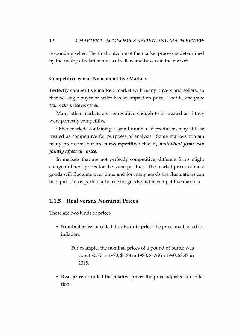
Example 2.1 D(p) = 60 − 4p. Then p = −1/4D(p) + 15 with slope = −14 .
28 CHAPTER 2. MARKET ANALYSIS
slope=
D(P)
14
15
60
-
Figure 2.4 A numerical example of linear demand function
Above, we have imposed the assumption that all other influences on
quantity demanded are held constant as the price changes. Price change
is the only cause of a change in quantity demanded (movement along de-
mand curve).
Changes in Quantity Demanded versus Changes in Demand
(1) Change in quantity demanded:
• i) caused by a change in price;
• ii) represented by a movement along the demand curve.
q
p
O q
p
O
Increase in Quantity Demanded Decrease in Quantity Demanded
Figure 2.5 Change in quantity demanded: movement along the demandcurve
(2) Change in demand:

2.1. DEMAND 29
• i) caused by a change in something other than price;
• ii) represented by a shift of the demand curve.
q
p
O q
p
O
“ increase in demand”
D
D
“ decrease in demand”
‘
D
D
‘
Figure 2.6 Change in demand: the shift of demand curves
Factors causing a change in demand (i.e., factors which shift the demand
curve):
a) Size of market as city grows.
E.g., Better marketing ⇒ increase in the number of consumers
⇒ increase in demand as depicted in Figure 2.7.
D D
‘
Figure 2.7 Demand curve shifts towards the right
b) Income.

30 CHAPTER 2. MARKET ANALYSIS
• Normal goods: As income rises, demand rises; most
goods are “normal” goods as also depicted in Figure
2.7.
• Inferior goods: As income rises, demand falls; e.g.,
potatoes, bread (poverty goods) as depicted in Figure
2.8.
D� D�
Figure 2.8 Demand curve shifts towards the left
c) Prices of related goods.
• substitute goods (called “competing goods”): Two good-
s for which an increase in the price of one leads to an
increase in the demand of the other, e.g., butter and
margarine as depicted in Figure 2.9.
— Price of margarine rises ⇒ will substitute butter ⇒demand for butter rises.
2.1. DEMAND 31
D D!
O
p
q
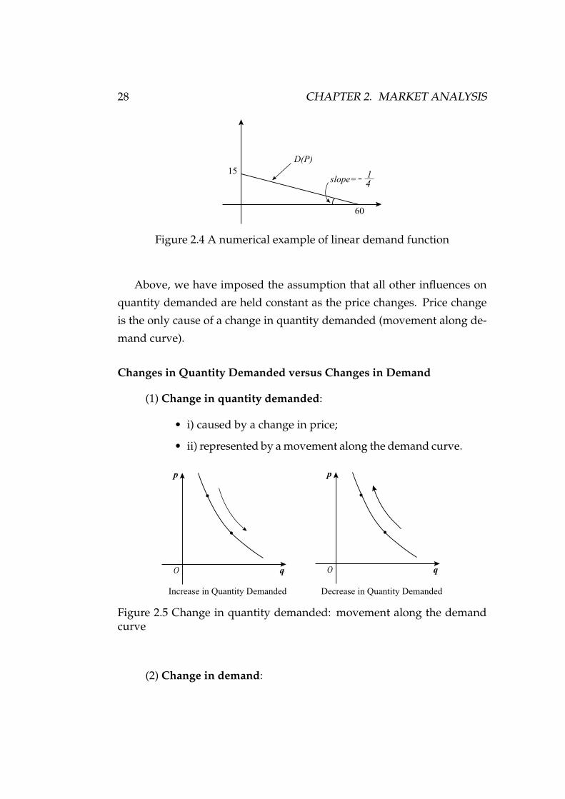
Figure 2.9 Demand curve shifts towards the right
• complementary goods: Two goods for which an in-
crease in the price of one leads to a decrease in the de-
mand of the other, e.g., hamburger and buns as depict-
ed in Figure 2.10.
—The price of hamburgers falls ⇒ quantity demanded
rises ⇒ demand for buns rises.
D�D�
O
p
q
Figure 2.10 Demand curve shifts towards the right
d) Tastes (preferences)
e.g., cigarette causes cancer ⇒ demand for cigarette falls as de-
picted in Figure 2.11.

32 CHAPTER 2. MARKET ANALYSIS
D� D�
O
p
q
Figure 2.11 Demand curve shifts towards the left
e) Expectations
e.g., paper towels go on sale next week ⇒ people will buy them
next week ⇒ demand of this week falls as depicted in Fig-
ure 2.12.
D D!
O
p
q
Figure 2.12 Demand curve shifts towards the left
f) Environmental conditions
e.g., weather conditions affect demand for air conditioners, ice
cream, and winter coats.

2.2. SUPPLY 33
2.2 Supply
Supply [S(p)]: a schedule which shows the relationship between the quan-
tity of a good that producers are willing and able to sell and the price of
the good, ceteris paribus.
The supply curve, labeled S, shows how the quantity of a good offered
for sale changes as the price of the good changes. The supply curve is
upward sloping: The higher the price, the more firms are able and willing
to produce and sell.
Market supply : The sum of supplies of individual firms.
price of calculators quantity supplied (millions) of calculators per year$20 600$10 300$2 100
O
p
q
10
20
S
100 300 600
Figure 2.13 A supply curve
Law of Supply: A direct relationship between price and quantity sup-
plied. That is, keeping other factors constant, the higher the price, the
larger will be the quantity supplied, and vice versa.
Linear supply function:
S(p) = ap + b.

34 CHAPTER 2. MARKET ANALYSIS
Direct relationship ⇒ a > 0.
Example 2.2 S(p) = −10 + 6p. Then, p = 16S(p) + 5
3 with slope = 16 .
O
p
q
S
-10
10
6
Figure 2.14 A numerical example of supply curve
Why a direct relationship? — Substitution of Expansion in Produc-
tion:
As the price of a good rises producers will shift resources into the pro-
duction of this relatively high priced good and away from production of
relatively low priced goods. Alternatively, the producers have incentives
to hire extra resources.
Changes in Quantity Supplied versus Changes in Supply
(1) Change in quantity supplied:
• i) caused by a change in price;
• ii) represented by a movement along the supply curve.
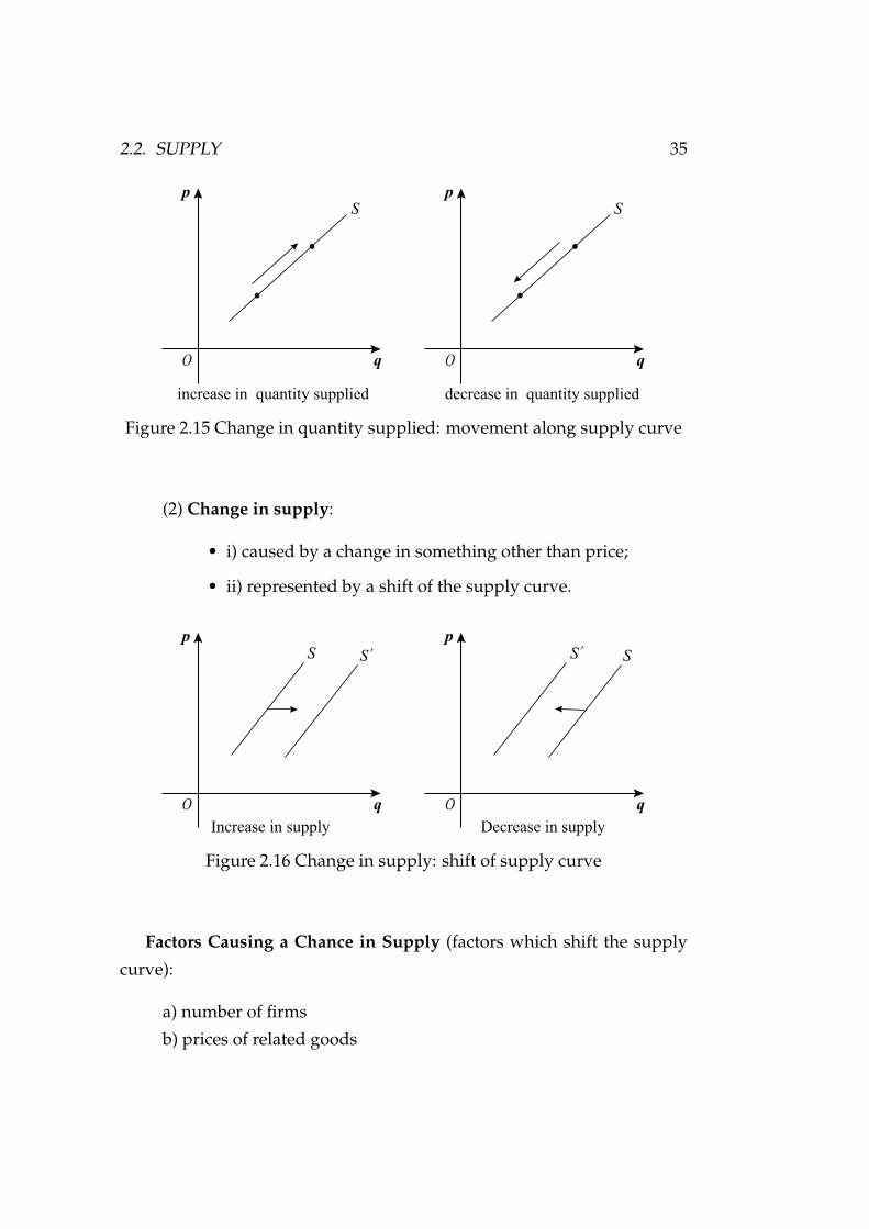
2.2. SUPPLY 35
S
O
p
q
S
O
p
q
increase in quantity supplied decrease in quantity supplied
Figure 2.15 Change in quantity supplied: movement along supply curve
(2) Change in supply:
• i) caused by a change in something other than price;
• ii) represented by a shift of the supply curve.
O
p
q
S
‘
S
O
p
q
S
‘
S
Increase in supply Decrease in supply
Figure 2.16 Change in supply: shift of supply curve
Factors Causing a Chance in Supply (factors which shift the supply
curve):
a) number of firms
b) prices of related goods

36 CHAPTER 2. MARKET ANALYSIS
c) technology
d) expectations
e) environmental conditions
Examples of change in supply:
i) prices of resources: increase in wage ⇒ increase in costs of
production ⇒ decrease in supply.
ii) advancement in technology ⇒ decrease in costs of produc-
tion ⇒ increase in supply.
2.3 Determination of Equilibrium Price and Quan-
tity
Notations:
• qd is quantity demanded of commodity;
• qs is quantity supplied of commodity;
• p is the price of the commodity;
Equilibrium price (or market clearing price), denoted by (pe), is estab-
lished at the price where quantity demanded equals quantity supplied of
the commodity.
Three relevant concepts:
• Market mechanism: Tendency in a free market for price to change
until the market clears.
• Surplus: Situation in which the quantity supplied exceeds the quan-
tity demanded.
• Shortage: Situation in which the quantity demanded exceeds the
quantity supplied.

2.3. DETERMINATION OF EQUILIBRIUM PRICE AND QUANTITY 37
When can we use the supply-demand model?
• We are assuming that at any given price, a given quantity will be
produced and sold.
• This assumption makes sense only if a market is at least roughly com-
petitive, which means that both sellers and buyers should have little
market power — i.e., little ability individually to affect the market
price.
• Suppose instead that supply were controlled by a single producer —
a monopolist. If the demand curve shifts in a particular way, it may
be in the monopolist’s interest to keep the quantity fixed but change
the price, or to keep the price fixed and change the quantity.
Example 2.3 (Example on Calculator (continued)) From Table 2.1, we can
know the equilibrium price is pe = $10. We say that“pe clears the market”.
The equilibrium quantity: qe = 3000 (qe = qs = qd).
p qd (millions) qs (millions) surplus (+) or shortage (-)
$20 700 6000 +5300
$10 3000 3000 0
$2 6500 1000 -5500
Table 2.1: Market equilibrium of calculator.

38 CHAPTER 2. MARKET ANALYSIS
O
p
q
S(P)
D(P)
pe
qe
=10
=3000
Figure 2.17 The determination of equilibrium price and quantity
Example 2.4 Find the market equilibrium price pe and equilibrium quan-
tity qe of the following demand and supply.
D(p) = 80 − 4p,
S(p) = −10 + 6p.
O
p
q
pe
qe-10
20
Figure 2.18 Finding market equilibrium: a numerical example
p = 0 implies D(0) = 80 and S(0) = −10. qd = 0 implies p = 20, and
qs = 0 implies p = 10/6 = 5/3. We then can draw the demand curve and
supply curve as depicted in Figure 2.18, giving us the market equilibrium
price pe and equilibrium quantity qe.

2.4. MARKET ADJUSTMENT 39
Algebraically, equaling D(pe) = S(pe), we have
80 − 4pe = −10 + 6pe,
and thus
90 = 10pe,
which yields pe = 9.
Substituting pe = 9 into either the equation, we have
qe = D(pe) = S(pe) = 80 − 4 × 9 = 44.
2.4 Market Adjustment
The market adjustment mechanism works as follows:
• Suppose p > pe. Then qs > qd, yielding surplus. Producers compete
to extract the surplus by price cutting. Price falls implies that qs falls
and qd rises. Eventually qs = qd at pe.
• Suppose p < pe. Then qd > qs, yielding shortage. Consumers com-
pete and force p up, having qd falls and qs rises. Eventually qd = qs at
pe.
Changes in Supply and/or Demand: Effect on Equilibrium
Example 2.5 (a) Demand increases from D1 to D2.

40 CHAPTER 2. MARKET ANALYSIS
O
p
q
S
pe
D
D!
E!
E
A!
pe
qe
! qe
Figure 2.19 The effect of an increase in demand on market equilibrium:resulting in increase in both pe and qe
When demand increases (say, due to an increase in income) from D1 to
D2, we have qd > qs at original equilibrium price pe1, resulting in shortage,
which in turn results in price rises. Thus consumers move from A to E2,
and producers move from E1 to E2 as depicted in Figure 2.19.
Result: Demand rises implies that both pe and qe rise.
Example 2.6 (b) Supply increases from S1 to S2.
O
p
q
pe
D
E
E!
B
pe
!
qe
q
e
!
S!
S
Figure 2.20 The effect of an increase in supply on market equilibrium: re-sulting in decrease in pe and increase in qe
2.4. MARKET ADJUSTMENT 41
When supply increases (say, due to an increase in productivity or a de-
crease in cost of production) from S1 to S2, we have qs > qd at pe1, resulting
in surplus, which in turn results in price falls. Thus consumers move from
E1 to E2, and producers move from B to E2 as depicted in Figure 2.20.
Result:Increase in S ⇒ pe falls and qe rises.
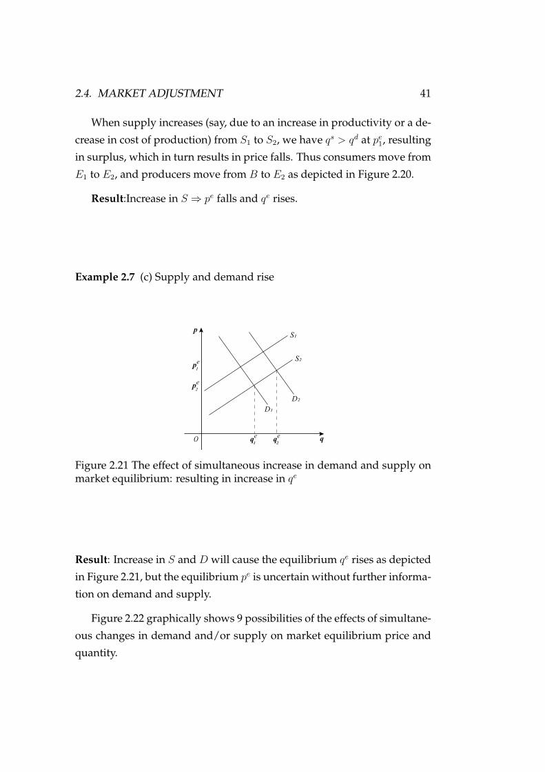
Example 2.7 (c) Supply and demand rise
O
p
q
pe
pe
!
qe
q
e
!
S!
S
D!
D
Figure 2.21 The effect of simultaneous increase in demand and supply onmarket equilibrium: resulting in increase in qe
Result: Increase in S and D will cause the equilibrium qe rises as depicted
in Figure 2.21, but the equilibrium pe is uncertain without further informa-
tion on demand and supply.
Figure 2.22 graphically shows 9 possibilities of the effects of simultane-
ous changes in demand and/or supply on market equilibrium price and
quantity.

42 CHAPTER 2. MARKET ANALYSIS
D
P
q
S
qe
Pe
D
P
q
S
qe
Pe
PS
D
P
q
S P
q
P
q
D
P
q
P
q
P
q
Demand is constant Demand increases Demand decreases
Supply
is constant
Supply
increases
Supply
decreases
D!!
"Pe
! qe"
D!
D
Pe!
"Pe
qe" qe
!
S!
qe! qe
"
Pe!
"Pe
S S!
D
D!
qe! qe
"
q
S S!
D!
D
Pe!
"Pe
qe!
S!
S
qe!qe
"
Pe!
"Pe
S S!
D
D!Pe!
"Pe
S
S!
D!
D
qe!qe
"
Pe!
Pe qe, Pe qe,
Pe qe, Pe qe,? Pe qe, ?
Pe qe, Pe qe, ? Pe qe,?
Figure 2.22 Nine possibilities of simultaneous change in demand and sup-ply
Note that as long as demand and supply both change (there are four
cases in Figure 2.22), either the equilibrium pe or quantity qe is uncertain.
Example 2.8 (Markets for eggs and college (continued)) From 1970 to 2010,
the real (constant-dollar) price of eggs fell by 55 percent, while the real
price of a college education rose by 82 percent.
The mechanization of poultry farms sharply reduced the cost of pro-
ducing eggs, shifting the supply curve downward. The demand curve for
eggs shifted to the left as a more health-conscious population tended to

2.4. MARKET ADJUSTMENT 43
avoid eggs. As a result, the real price of eggs fell sharply and egg con-
sumption rose as depicted in (a) Figure 2.23.
p
q5300 6392
$0.61
$0.27
S1970
S2016
D1970
D2016
(1970
dollars
per
dozen)
(million dozens)
p
q
(annual
cost in
1970
dollars)
(million of students enrolled)
(a) (b)
S2016
S1970
D1970
D2016
6.9 12.5
$3835
$2112
Figure 2.23 (a) Markets for eggs; (b) Markets for college
As for college, increases in the costs of equipping and maintaining
modern classrooms, laboratories, and libraries, along with increases in fac-
ulty salaries, pushed the supply curve up. The demand curve shifted to
the right as a larger percentage of a growing number of high school gradu-
ates decided that a college education was essential. As a result, both price
and enrollments rose sharply as depicted in (b) Figure 2.23.
Example 2.9 (Explaining wage inequality in the United States) Over the
past four decades, the wages of skilled high-income workers have grown
substantially, while the wages of unskilled low-income workers have fall-
en slightly.
From 1978 to 2009, people in the top 20 percent of the income distribu-
tion experienced an increase in their average real (inflation-adjusted) pre-
tax household income of 45 percent, while those in the bottom 20 percent
saw their average real pretax income increase by only 4 percent.
By 2016, the top 1% of Americans controlled a record-high 38.6% of the
country’s wealth, almost 2 times as much as bottom 90%. The top 10%

44 CHAPTER 2. MARKET ANALYSIS
of Americans own almost 70% of the country’s total wealth while the top
20% of Americans owned 86% of the country’s wealth and the bottom 80%
of the population owned 14% in 2020.
Why? One of reasons is the differences in human capital and new
technological revolution (such as artificial intelligence, digital economy,
etc.). While the supply of unskilled workers (with limited educations) has
grown substantially, the demand for them has risen only slightly.
On the other hand, while the supply of skilled workers — e.g., engi-
neers, scientists, managers, and economists — has grown slowly, the de-
mand has risen dramatically, pushing wages up.
Example 2.10 (Supply and Demand for City Office Space) Since COVID-
19, the supply for city office decreases slightly, but the demand decreases
substantially (people work from home), so that the average rental price for
office fell.
2.5 Elasticity of Demand and Supply
The concept of elasticity has immense importance in consumer’s consump-
tion decisions, businessmen’s pricing strategies, government policies (such
as taxation), and international trade (such as the term of trade between t-
wo countries).
Elasticity measures responsiveness of percentage change in quantity
demanded (or supplied) to a percentage change in a variable (such as own
price, prices of other goods, income).
Can we use slope of the curve to measure the elasticity? No, because
a change in scale can make a curve look flatter or steeper without altering
absolute responsiveness. Thus, changing units (say from a dollar to a cent)
will alter the slope. For this reason, economists use a unitless measure to
measure the elasticity.

2.5. ELASTICITY OF DEMAND AND SUPPLY 45
2.5.1 Elasticity of Demand
Price elasticity of demand (“own” Price Elasticity): Percentage change in
quantity demanded resulting from a percentage change in its price:
Epd = percentage change in quantity demanded
percentage change in its price
= ∆q(p)/q(p)∆p/p
,
where “∆” = “change”. Since demand curves in general slope downward,
Epd will be negative.
Range of Value for Epd :
(a) Inelastic demand: |Epd | < 1.
| ∆qx/qx
∆px/px
| < 1 ⇒ |∆qx/qx| < |∆px/px|.
When demand is inelastic, the quantity demanded is rela-
tively unresponsive to changes in price; e.g., cigarettes.
(b) Elastic demand: |Epd | > 1. That is |∆qx/qx| > ||∆px/px|.
When demand is elastic, the quantity demanded is relative-
ly responsive to changes in price; e.g., automobiles in the
short run, competing goods.
(c) Unit elasticity of demand: |Epd | = 1, i.e., |∆qx/qx| = |∆px/px|.
(d) Iso-elastic demand curve Demand curve: the price elastic-
ity is constant.
(e) Perfectly inelastic demand: |∆qx/qx| = 0 for all changes in
price —i.e., totally unresponsive.
(f) Perfectly elastic demand: |Epd | = ∞. A very small per-
centage change in price leads to a tremendous percentage
change in quantity demanded.

46 CHAPTER 2. MARKET ANALYSIS
P
qOE =0P
d
P
qO
P
qO
P
qO
P
qOE = ∞P
d
D
D
D
D
D
E <1P
d E =1P
d
E >1P
d
Figure 2.24 Types of demand elasticity
Example 2.11 We first suppose that the price px of good x increases from
$1 to $2 and the quantity demanded qx changes from 10 to 5.
px qx
$1 10
$2 5
We then have ∆qx/qx = −50%, ∆px/px = 100%, and thus Epd = − 50
100 =−1
2 .
Now suppose that the price decreases from $2 to $1 and the quantity
demanded changes from 5 to 10.
px qx
$2 5
$1 10

2.5. ELASTICITY OF DEMAND AND SUPPLY 47
∆qx/qx = 100%, ∆px/px = 1−22 = −50%, so Ep
d = −2.
This demonstrates how Epd varies according to the p-q combination
which is used as a reference point. To avoid this problem, we use the
midpoint elasticity, also called the arc elasticity of demand.
Midpoint ( arc ) elasticity of demand: Epd between points (px, qx) and
(px′, qx
′) is given by
Epd =
∆qx/12(qx + qx
′)∆px/1
2(px + px′)
.
This just uses the midpoints as the reference points.
Example 2.12 (Example 2.11 (continued)) Consider the example again.
px qx
$2 5
$1 10
Note that
∆qx/12
(qx + qx′) = − 5
12 · 15
= −23
and
∆px/12
(px + px′) = 1
12 · 3
= 23
,
so we have
Epd = 2/3
2/3= −1.
Only very special demand curves have constant elasticity between any
two points.
A straight line demand function
qx = a − bp,

48 CHAPTER 2. MARKET ANALYSIS
does not have a constant elasticity throughout. Indeed,
Epd = ∆qx/qx
∆px/px
= px
qx
· ∆qx
∆px
= px
qx
× the slope of qx
= a × px
qx
= constant
because px
qxis not constant even though the slope of a linear demand curve,
a, is constant.
Therefore, along a downward-sloping straight-line demand curve, the
price elasticity varies, but the slope is constant.
Elasticity along Straight Line Demand Curve
Since slope of straight line is constant (i.e., ∆qx
∆pxis constant), | ∆qx
∆px| = LB
AL. So
we have
|Epd | = |∆qx
∆px
| · px
qx
= LB
AL· OL
LB= OL
AL.
xO
Px
A
B
C
L
} }
E >1P
d
E <1P
d
Figure 2.25 Elasticity along a linear demand curve

2.5. ELASTICITY OF DEMAND AND SUPPLY 49
Thus if B is the midpoint of the demand curve, then |Epd | = 1. If B is a
point above the midpoint, then AL < OL ⇒ |Epd | > 1. If B is a point below
the midpoint, AL > OL ⇒ |Epd | < 1.
2.5.2 Elasticity and Total Expenditure
The total expenditure (TE) for consuming a good is:
TE = px × qx.
Along a demand curve, we have: qx falls as px rises. We are now inter-
ested in what will happen to the total expenditure px × qx. Since px and qx
are inversely related by the law of downward-sloping demand, we need
information about the magnitude of the changes in px and qx to determine
the direction of the effect on px × qx. To do this, we use the price elasticity
of demand. They have the following relationships:
|Epd | > 1 |Ep
d | < 1 |Epd | = 1
px rises TE falls TE rises TE holds constant
Table 2.2: The relationship between elasticity and total expenditure.
E >1P
d
x
P
A
B
x’ x
Px
Px’
D
x
P
A
B
x’ x
Px
Px’
D
E =1P
d
x
P
A
B
x’ x
Px
Px’
D
E <1P
d
Figure 2.26 Total expenditure under alternative demand elasticities

50 CHAPTER 2. MARKET ANALYSIS
In other words, when demand is elastic, price and total expenditure
move in opposite directions. When demand is inelastic, price and total
expenditure move in the same direction. When demand is unit elastic,
total expenditure maintains constant when the price varies.
Algebraically, we can verify that these relationships hold true. Suppose
|Epd | > 1 and px
′ > px.
∆qx/12(qx + qx
′)∆px/1
2(px + px′)
> 1
⇒ ∆qx
qx + qx′ >
∆px
px + px′
⇒(qx − qx′)(px + px
′) > (px′ − px)(qx + qx
′)
⇒pxqx − px′qx
′ > −pxqx + px′qx
′
⇒2pxqx > 2px′qx
′
⇒pxqx > px′qx
′.
This shows that if px rises, the total expenditure falls.
Other Elasticities:
• Income elasticity (EId):
EId = ∆Dx/Dx
∆I/I.
• Cross-price elasticity of demand: Let py be the price of good y. The
cross-price elasticity of demand for x with respect to the price is de-
fined as
Epy
dx= ∆Dx/Dx
∆py/py
.

2.5. ELASTICITY OF DEMAND AND SUPPLY 51
2.5.3 Price Elasticity of Supply
The Price Elasticity of Supply: a measure of the responsiveness of
quantity supplied to a change in price. It is defined as the percentage
change in quantity supplied divided by the percentage change in
price:
EPS = ∆S(P )/S(P )
∆P/P= P
S(P )× ∆S(P )
∆P= P
S(P )× the slope of S(P ).
We have the following typical cases:
– EPS > 0 when supply slopes upwards.
– If EPS > 1, then supply is elastic.
– If EPS < 1, then supply is inelastic.
– If EPS = 1, then supply is unit elastic.
– If EPS = 0, then supply is perfectly inelastic.
– If EPS = ∞, then supply is perfectly elastic.
S(P)P
q qE =0ps
P
S(P)
E = ∞ps
Figure 2.27 Perfectly inelastic and perfectly elastic supplies
Example 2.13 (Market for Wheat) During recent decades, changes in the
wheat market had major implications for both American farmers and U.S.
agricultural policy.

52 CHAPTER 2. MARKET ANALYSIS
To understand what happened, let’s examine the behavior of supply
and demand beginning in 1981.
Qs = 1800 + 240P
Qd = 3550 − 266P
By setting the quantity supplied equal to the quantity demanded, we can
determine the market-clearing price and the equilibrium quantity of wheat
for 1981:
P = $3.46,
and
Q = 2630.
We use the demand curve to find the price elasticity of demand:
EPD = P∆QD
Q∆P= 3.46
2630(−266) = −0.35
and so demand is inelastic.
We can likewise calculate the price elasticity of supply
EPS = P∆QS
Q∆P= 3.46
2630(240) = 0.36.
Suppose that a drought caused the supply decreases significantly, which
pushes the price up to $4.00 per bushel. In this case, the quantity demand-
ed would fall to 3550 - (266)(4.00) = 2486 million bushels. At this price and
quantity, the elasticity of demand would be
EPD = P∆QD
Q∆P= 4.00
22800(−266) = −0.43
In 2007, demand and supply were
Qs = 1400 + 115P

2.5. ELASTICITY OF DEMAND AND SUPPLY 53
Qd = 2900 − 125P
The market-clearing price and the equilibrium quantity are then
P = $6,
and
Q = 2150.
Dry weather and heavy rains, combined with increased export demand
caused the price to rise considerably. You can check to see that, at the 2007
price and quantity, the price elasticity of demand was -0.35 and the price
elasticity of supply 0.32. Given these low elasticities, it is not surprising
that the price of wheat rose so sharply.
2.5.4 Short-Run versus Long-Run Elasticities
Consumption of Durables and Nondurables
Annual growth rates are compared for GDP, consumer expenditures on
durable goods (automobiles, appliances, furniture, etc.), and consumer ex-
penditures on nondurable goods (food, clothing, services, etc.).
Because the stock of durables is large compared with annual demand,
short-run demand elasticities are larger than long-run elasticities. Like
capital equipment, industries that produce consumer durables are “cycli-
cal” (i.e., changes in GDP are magnified).
This is not true for producers of nondurables.
Income Elasticity
Income elasticities also differ from the short run to the long run. For most
goods and services-foods, beverages, fuel, entertainment, and so on— the
income elasticity of demand is larger in the long run than in the short run.

54 CHAPTER 2. MARKET ANALYSIS
For a durable good, the opposite is true. The short-run income elastic-
ity of demand will be much larger than the long-run elasticity.
Example 2.14 (Demand for Gasoline and Automobiles) Consider the price
elasticities of demand for gasoline and automobiles.
Elasticity for Gasoline 1 2 3 5 10price -0.2 -0.3 -0.4 -0.5 -0.8
income 0.2 0.4 0.5 0.6 1.0
Table 2.3: Demand for gasoline: Number of years allowed to pass follow-ing a price or income change
Elasticity for Automobiles 1 2 3 5 10price -1.2 -0.9 -0.8 -0.6 -0.4
income 3.0 2.3 1.9 1.4 1.0
Table 2.4: Demand for automobiles: Number of years allowed to pass fol-lowing a price or income change
In the short run, an increase in price has only a small effect on the
quantity of gasoline demanded. Motorists may drive less, but they will
not change the kinds of cars they are driving overnight. In the longer run,
however, because they will shift to smaller and more fuel-efficient cars, the
effect of the price increase will be larger. Demand for gasoline, therefore,
is more elastic in the long run than in the short run.
The opposite is true for automobile demand. If price increases, con-
sumers initially defer buying new cars; thus annual quantity demanded
falls sharply. In the longer run, however, old cars wear out and must be
replaced; thus annual quantity demanded picks up. Demand for automo-
biles, therefore, is less elastic in the long run than in the short run.
2.6. EFFECTS ON GOVERNMENT INTERVENTION: PRICE CONTROLS55
2.6 Effects on Government Intervention: Price Con-
trols
Markets can be thought of as a self-adjustment mechanism; they auto-
matically adjust to any change affecting the behavior of buyers and sellers
in the market. But for this mechanism to operate effectively, the price must
be free to move in response to the interplay of supply and demand. When
the government steps in to regulate prices, the market does not function
in the same way.
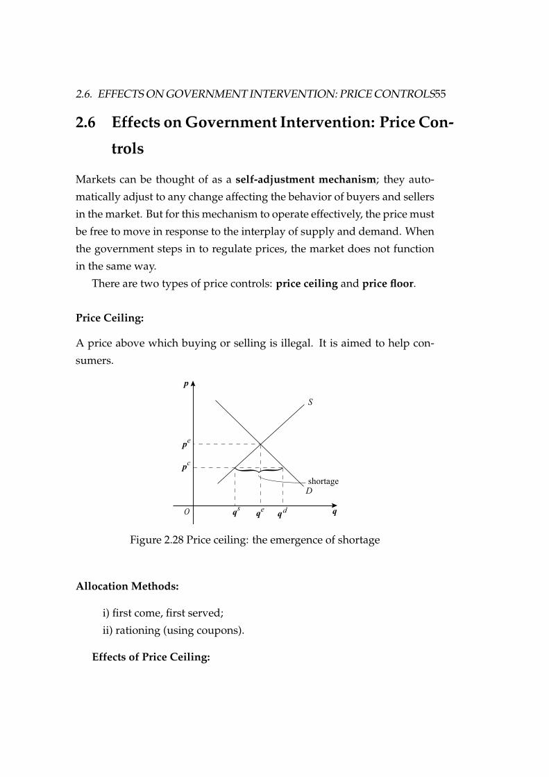
There are two types of price controls: price ceiling and price floor.
Price Ceiling:
A price above which buying or selling is illegal. It is aimed to help con-
sumers.
O
p
q
pe
qe
qd
D
S
qs
pc {
shortage
Figure 2.28 Price ceiling: the emergence of shortage
Allocation Methods:
i) first come, first served;
ii) rationing (using coupons).
Effects of Price Ceiling:

56 CHAPTER 2. MARKET ANALYSIS
a. in general it results in shortage;
b. there is a tendency to form a black market;
c. bad service and bad quality of goods;
d. production is reduced;
e. provide wrong information about production and consump-
tion;
f. it hurts producers who provide goods, and some consumers
gain from the price ceiling but other may be worse off.
Price Floor (also called the Price Support):
A price below which buying or selling is prohibited. It is aimed to help
producers. Examples include setting prices of agricultural products and
minimum wage rate.
O
p
q
pe
qe
qd
D
S
qs
pf
{surplus
Figure 2.29 Price floor: the emergence of surplus
Effects of Price Floor:
a. in general it results in surplus;
b. provide unnecessary service;
c. lead to over investment;
d. provide wrong information about production and consump-
tion.

2.6. EFFECTS ON GOVERNMENT INTERVENTION: PRICE CONTROLS57
Methods for Maintaining Price Support:
i) the government purchases surplus, and then the total rev-
enue of the producer = pf × qs.
ii) output is restricted at qd, and then the total revenue of the
producer = pf × qd.
Besides the effects mentioned for these two types of price controls, we
will discuss they also result in welfare losses.
Example 2.15 (Price Control and Wheat) Suppose that the demand and
supply of wheat are respectively given by
D(p) = 90 − 20p,
S(p) = −15 + 10p.
a) Find the market equilibrium price and quantity.
Setting D(p) = S(p), we have 90 − 20p = −15 + 10p which gives us
pe = 105/30 = 3.5 and qe = 20.
b) Suppose a price support is set at $4. What is the surplus?
Since
D(4) = 90 − 20 × 4 = 10,
S(4) = −15 + 10 × 4 = 25,
so the surplus is given by
S(4) − D(4) = 25 − 10 = 15.

58 CHAPTER 2. MARKET ANALYSIS

Part II
Demand Side of Market
59


61
Part 2 presents theoretical core of consumer behavior and individual
and market demands.

62

Chapter 3
Theory of Consumer Choice
This chapter discusses the theory of consumer choice – a bedrock founda-
tion of economics. It resides at the center of how economists think, and
can be viewed as a typical situation of how an individual makes an inde-
pendent decision. In practice, corporate policy and public policy require
an understanding of the theory of consumer behavior: the explanation of
how consumers allocate incomes to the purchase of different goods.
A consumer can have numerous characteristics, such as preferences,
gender, appearance, age, lifestyle, wealth, ability, and so on. Which of
the above are critical in determining the consumer’s optimal choice? In
principle, a consumer’s choice is determined by the consumer’s subjective
preference subject to objective restrictions, typically, budget constraints.
3.1 Budget Constraints
Budget constraints: Constraints that consumers face as a result of limited
incomes.
3.1.1 Budget Line
The budget line: A straight line representing all possible combinations
of goods that a consumer can obtain at given prices by spending a given
63

64 CHAPTER 3. THEORY OF CONSUMER CHOICE
income, namely, the total expenditure of consumptions is equal to income.
A budget line with two commodities, as depicted in Figure fig3-2, is:
px × x + py × y = I, (3.1)
where px and py represent prices of goods x and y, and hence px ×x+py ×y
stands for total expenditure which is equal to income I .
y
xO
IPy
IPx
affordable
bundle
unaffordable
bundle
budget line
slope=PxPy
Figure 3.1 Budget constrains and budget line
We can rewrite the budget line (3.1) as
y = I
py
− px
py
× x, (3.2)
where the slope of (3.1) is −px
py, y-axis intercept is I
py, and x-axis intercept is
Ipx
.
Example 3.1 Two goods x and y, with prices px = 10 and py = 5. Income
is I = 100. So the budget line is
10x + 5y = 100.
The slope of budget line is −px
py= −10/5 = −2, y-axis intercept is I
py=

3.1. BUDGET CONSTRAINTS 65
Ipy
= 100/5 = 20, and x-axis intercept is Ipx
= 100/10 = 10.
Combination: px× unit of x + py × unit of y = income
a. 10 × 10 + 5 × 0 = $100
b. 10 × 8 + 5 × 4 = $100
c. 10 × 6 + 5 × 8 = $100
d. 10 × 4 + 5 × 12 = $100
e. 10 × 2 + 5 × 16 = $100
b. 10 × 0 + 5 × 20 = $100
O
y
x
a
b
c
d
f
e
Figure 3.2 A budget line with two consumption goods
3.1.2 Changes in Budget Line
What if prices and income increase at the same rate? If we double both
prices and income, then 2pxx + 2pyy = 2I , and nothing changes.

66 CHAPTER 3. THEORY OF CONSUMER CHOICE
y
xO 10
10
20
-2
Figure 3.3 The effect of a change in price on budget line
What if only one price changes? If py is changed to p∗y = 10, and px
and I are the same as before, the new budget line is 10x + 10y = 100, with
slope −px
py= −1. That is, a change in the price of one good (with income
unchanged) causes the budget line to rotate about one intercept.
y
xO 10
20
30
15
10x+5y=150
10x+5y=100
Figure 3.4 The effect of a change in income on budget line
What if only income changes? If the income changes from $100 to $150,
the new budget line is 10x+5y = 150. Then a change in income (with prices
unchanged) causes the budget line to shift parallel to the original line.

3.2. CONSUMER PREFERENCES 67
3.2 Consumer Preferences
The consumer is assumed to have preferences over bundles of goods. Sup-
pose that there are 2 goods available, x and y, and two bundles of these
goods, A and B, where each bundle contains a given amount of x and y:
A = (xA, yA), B = (xB, yB).
y
xO
bundle A
bundle B
xA xB
yB
yA
Figure 3.5 Two alternative consumption bundles A and B
3.2.1 Basic Assumptions on Preferences
We make the following assumptions on the consumer’s preferences.
i ) Completeness: consumers can compare and rank all possi-
ble baskets. Between any two bundles, the consumer can
only make one of the following statements:
A is preferred to B (A ≻ B),
B is preferred to A (B ≻ A), or
A is indifferent to B (A ∼ B).
By indifferent we mean that the consumer will be equally
satisfied with either basket. Note that these preferences ig-

68 CHAPTER 3. THEORY OF CONSUMER CHOICE
nore costs. A consumer might prefer steak to hamburger
but buy hamburger because it is cheaper.
ii ) Transitivity:
A ≻ B and B ≻ C imply A ≻ C.
Transitivity is normally regarded as necessary for consumer
consistency.
iii ) More is preferred to less: goods are assumed to be desir-
able — i.e., to be good;
if A = (xA, yA), B = (xA, yA + c), c > 0, then
B ≻ A.
Consequently, consumers always prefer more of any good
to less. In addition, consumers are never satisfied or satiat-
ed; more is always better, even if just a little better.
Indifference curve: a curve representing all combinations of market
baskets that provide a consumer with the same level of satisfaction.. Thus,
a consumer is indifferent between any two bundles that lie on the same
indifference curve.
y
xO
A
BA’
indifference curve
Figure 3.6 The process of formulating an indifference curve

3.2. CONSUMER PREFERENCES 69
To find an indifference curve, start at bundle A. Subtracting one unit
of good y, puts us at a point A′, strictly less preferred to A by assumption
iii), i.e., A′ ≺ A. However, if we add more x to A′, we know that A′ will be
less preferred to the resulting new point. If we add “enough” x to A′, then
we find a point B such that A ∼ B, as shown in Figure 3.6, etc.
Similarly, we can trace out a family of indifference curves, namely, an
indifference map — i.e., a graph containing a set of indifference curves
showing the market baskets among which a consumer is indifferent. In
Figure 3.7, we have A ∼ B, A ∼ B, ¯A ∼ ¯B, but any point on U1 is preferred
to any point on U0, and is less preferred to any point on U2 by assumptions
ii) and iii).
y
xO
A
B
A
B
A
B
U
U!
U"
Figure 3.7 Indifference map: a set of indifference curves
3.2.2 Properties of Indifference Curves
There are two crucial properties of indifference curves:
i) Indifference curves slope downward by assumption ii).
ii) Indifference curves cannot intersect.

70 CHAPTER 3. THEORY OF CONSUMER CHOICE
Suppose they did intersect, note that A ∼ B, C ∼B, C ≻ A ⇒ C ≻ B but C ∼ B, hence a
contradiction.
y
xO
A
B
C
Figure 3.8 Indifference curves cannot intersect
3.2.3 Marginal Rate of Substitution
The slope of an indifference curve reveals the so-called marginal rate of
substitution of one good for another good.
The marginal rate of substitution of x for y (MRSxy): Represent the
maximum of units of y that must be given up for one extra unit of x if the
consumer is to remain indifferent.
Formally, MRSxy =∣∣∣∆y
∆x
∣∣∣ is the absolute value of the slope of the indif-
ference curve, where“∆” stands for small changes. That is, the magnitude
of the slope of an indifference curve measures the consumer’s marginal
rate of substitution (MRS) between two goods x and y.
Observe that the MRS falls as we move down the indifference curve.
The decline in the MRS reflects convexity of consumer preferences:
Strict Convexity: Indifference curves are strictly convex to the origin,
which yields diminishing marginal rate of substitution, as depicted in Fig-
ure 3.9.
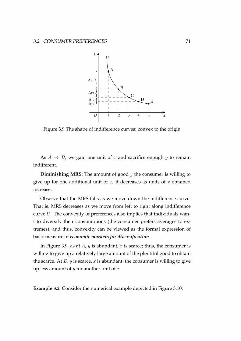
3.2. CONSUMER PREFERENCES 71
y
xO
A
B
C
DE
{{{{
U
∆y!
∆y"
∆y#∆y$
1 2 3 4 5
Figure 3.9 The shape of indifference curves: convex to the origin
As A → B, we gain one unit of x and sacrifice enough y to remain
indifferent.
Diminishing MRS: The amount of good y the consumer is willing to
give up for one additional unit of x; it decreases as units of x obtained
increase.
Observe that the MRS falls as we move down the indifference curve.
That is, MRS decreases as we move from left to right along indifference
curve U . The convexity of preferences also implies that individuals wan-
t to diversify their consumptions (the consumer prefers averages to ex-
tremes), and thus, convexity can be viewed as the formal expression of
basic measure of economic markets for diversification.
In Figure 3.9, as at A, y is abundant, x is scarce; thus, the consumer is
willing to give up a relatively large amount of the plentiful good to obtain
the scarce. At E, y is scarce, x is abundant; the consumer is willing to give
up less amount of y for another unit of x.
Example 3.2 Consider the numerical example depicted in Figure 3.10.

72 CHAPTER 3. THEORY OF CONSUMER CHOICE
Clothing
O
U
Food
(5,30)
(10,18)
(15,13)(20,10)
(25,8)
5 10 15 20 25
30
18
13
108
Figure 3.10 MRS between clothing and food
Clothing (C) Food (F) MRS of F for C30 518 10 |∆C
∆F | = 30−1810−5 = 2.4 ↓
13 15 |∆C∆F | = 18−13
15−10 = 1.0 ↓10 20 |∆C
∆F | = 13−1020−15 = 0.6 ↓
8 25 |∆C∆F | = 10−8
25−20 = 0.4 ↓7 30 |∆C
∆F | = 8−730−25 = 0.2 ↓
3.2.4 Special Shapes of Indifference Curves:
An indifference curve is generally convex to the origin although it may not
be strictly convex to the origin. This may be true for some special shapes
of indifference curves.
i) Perfect substitutes (linear indifference curves): Since the slope of a
straight line is constant, MRS is constant.

3.2. CONSUMER PREFERENCES 73
y
xO
U U!
Figure 3.11 Perfect substitutes: constant MRS
ii) Perfect complements: two goods for which the MRS is zero or infi-
nite; the indifference curves are shaped as right angles, e.g., x = left shoe,
y = right shoe.
y
xO
U
U!
Figure 3.12 Perfect complements: shaped as right angles
iii) Only the consumption of good y matters; see Figure 3.13.

74 CHAPTER 3. THEORY OF CONSUMER CHOICE
y
xO
U�
U�
Figure 3.13 Horizontal indifference curves
iv) Only the consumption of good x matters; see Figure 3.14.
y
xO
U U!
Figure 3.14 Vertical indifference curves
v) Bads: Bad good for which less is preferred rather than more; see Fig-
ure 3.15.

3.2. CONSUMER PREFERENCES 75
O
y
x
u
u!
u"
Figure 3.15 Vertical indifference curves
3.2.5 Utility Functions
Indifference curves, which represent consumer preferences, enable us to
rank commodity bundles. That is, as shown in Figure 3.16, A ≺ B, and
B ≺ C. Sometimes it is convenient to summarize these rankings with a
numerical score. Therefore, #1 = C, #2 = B, #3 = A.
y
xO
A
B
U
U!
U"
C
Figure 3.16 Ranking alternative market baskets using indifference curves
A utility function can be derived by a set of indifference curves, each

76 CHAPTER 3. THEORY OF CONSUMER CHOICE
with a numerical indicator, which represents the consumer’s preferences.
That is, U(x, y) assigns a number to commodity bundle (x, y) such that
whenever
(a) U(x, y) > U(x, y), then bundle (x, y) is preferred to bundle
(x, y).(b) U(x, y) = U(x, y), then the consumer is indifferent between
(x, y) and (x, y).
Thus U(x, y) can be used to rank commodity bundles. Such a func-
tion is called the ordinal utility function. The difference of ordinal utility
function relative to cardinal utility function can be described as follows:
• Ordinal utility function: Utility function that generates a ranking of
market baskets in order of most to least preferred.
• Cardinal utility function: Utility function describing by how much
one market basket is preferred to another.
Example 3.3 (Can Money Buy Happiness?) A cross-country comparison
shows that individuals living in countries with higher GDP per capita are
on average happier than those living in countries with lower per-capita
GDP.
To find an indifferent curve from a utility function, we provide the fol-
lowing examples:
Example 3.4 Suppose
U(x, y) = x + 2y.
Along an indifferent curve the consumer is indifferent between alterna-
tive bundles. That is, along an indifference curve U(x, y) = U is constant.
Suppose U1 = 10. To trace an indifference curve, we find all combina-
tions of (x, y) which satisfy U(x, y) = U1 = 10 ⇒ x + 2y = 10.
Suppose U2 = 15 ⇒ x + 2y = 15.

3.2. CONSUMER PREFERENCES 77
y
xO
U�=10
U�=15
5
Figure 3.17 Tracing linear indifference curves
Since U(x, y) = 10 < U(x, y) = 15, the latter indifference curve rep-
resents bundles preferred to the original set. That is consistent with the
indifference curve being further from the origin.
Example 3.5 Suppose
U(x, y) = xy.
y
xO
U=50
2 5 10 25
2
5
10
25
Figure 3.18 Tracing convex indifference curves
At U = 50 ⇒ xy = 50. Bundles which satisfy this equation include

78 CHAPTER 3. THEORY OF CONSUMER CHOICE
• x = 25 and y = 2,
• x = 10 and y = 5,
• x = 5 and y = 10,
• x = 2 and y = 25.
Computing MRS from a Utility Function
If we know a particular utility function, we can compute MRS of the cor-
responding indifference curve. Indeed, along an indifference curve repre-
sented by a utility level U , we have ∆U = 0, hence
0 = MUx × ∆x + MUy × ∆y.
We then have∆y
∆x= −MUx
MUy
.
Since the slope of the indifference curve is ∆y∆x
= −MRSx,y, we thus
have
MRSx,y = MUx
MUy
.
Example 3.6 (Example 3.4 continued) Suppose
U(x, y) = x + 2y.
Then we have
MUx = 1, MUy = 2 ⇒ MRS = 12
.
Example 3.7 (Example 3.5 continued)
U(x, y) = xy
Let U = xy ⇒ y∆x + x∆y = 0 ⇒ ∆y∆x
= − yx
⇒ MRS = yx.
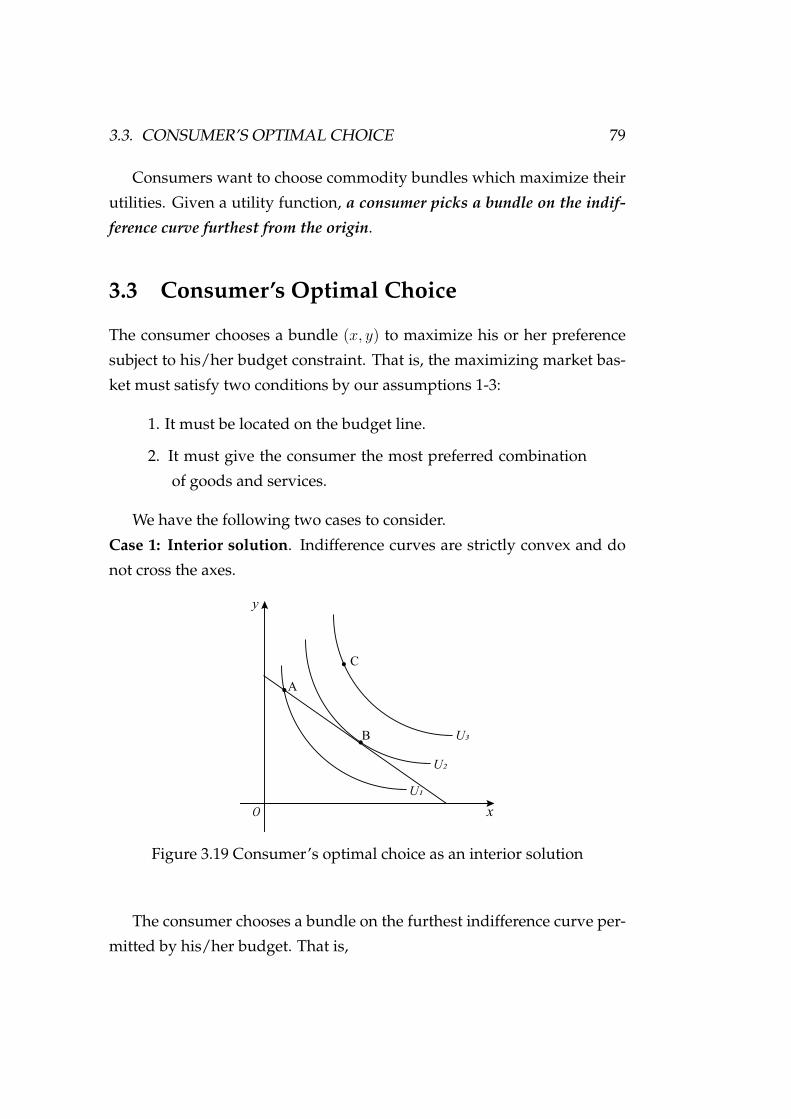
3.3. CONSUMER’S OPTIMAL CHOICE 79
Consumers want to choose commodity bundles which maximize their
utilities. Given a utility function, a consumer picks a bundle on the indif-
ference curve furthest from the origin.
3.3 Consumer’s Optimal Choice
The consumer chooses a bundle (x, y) to maximize his or her preference
subject to his/her budget constraint. That is, the maximizing market bas-
ket must satisfy two conditions by our assumptions 1-3:
1. It must be located on the budget line.
2. It must give the consumer the most preferred combination
of goods and services.
We have the following two cases to consider.
Case 1: Interior solution. Indifference curves are strictly convex and do
not cross the axes.
y
xO
A
B
U
U!
U"
C
Figure 3.19 Consumer’s optimal choice as an interior solution
The consumer chooses a bundle on the furthest indifference curve per-
mitted by his/her budget. That is,

80 CHAPTER 3. THEORY OF CONSUMER CHOICE
• C - too expensive and hence is not affordable for the consumer,
• B ≻ A,
• hence B is the utility-maximizing bundle; at this point, the budget
line and indifference curve U2 are tangent.
Thus, at the interior optimal bundle, the following two condition must
be satisfied:
(1) The slope of the indifference curve equals the slope of budget
line. Since the slope of indifference curve is −MRSxy and
the slope of the budge line is −px
py, at B, we have
MRSxy = px
py
. (3.3)
(2) The choice is on the budget line:
pxx + pyy = I. (3.4)
Put differently, at the point of satisfaction maximization,
the MRS between the two goods equals the price ratio, and
also satisfy the budget line. Thus, equations (3.3) and (3.4)
fully characterize the consumer’ interior optimal choice.
In other words, the underlying economic intuition can be analyzed us-
ing cost-benefit analysis. Note that marginal benefit is the benefit from the
consumption of one additional unit of a good and marginal cost is the cost
of one additional unit of a good. So, we can then say that satisfaction is
maximized when the marginal benefit — the benefit associated with the
consumption of one additional unit of food — is equal to the marginal
cost — the cost of the additional unit of food. The marginal benefit is mea-
sured by the MRS. We therefore arrive at the equal marginal principle,

3.3. CONSUMER’S OPTIMAL CHOICE 81
which states that utility is maximized when the consumer has equalized
the marginal utility per dollar of expenditure across all goods.
Since MRSxy = MUx
MUy, the marginal equality condition (3.3) can be rewrit-
ten asMUx
MUy
= px
py
, (3.5)
or equivalently,MUx
px
= MUy
py
, (3.6)
which means the marginal utility per dollar for x equals the marginal
utility per dollar for y.
Example 3.8 (Example 3.5 continued again) Suppose that a consumer’s u-
tility function is given by
U(x, y) = xy,
and the prices and income are given by
px = 2, py = 1, I = 100.
Note that MRS = yx. By (3.3), i.e., MRS = px
py, and (3.4), we have
(1) yx
= 21 ⇒ y = 2x.
(2) pxx + pyy = 100 ⇒ 2x + y = 100.
Substituting y = 2x from (1) into the budget line (2), we have
2x + 2x = 100
and then
4x = 100.
Thus, we have x∗ = 25 and y∗ = 50.
Case 2: Corner solution (e.g., linear Indifference Curve): Situation in
which the marginal rate of substitution for any good is not equal to the

82 CHAPTER 3. THEORY OF CONSUMER CHOICE
slope of the budget line. When a corner solution arises, the consumer
maximizes satisfaction by consuming only one of the two goods.
Example 3.9 (Example 3.4 continued again) Suppose U = x + 2y. Then
MRS = 12 . The optimal bundle depends on the slopes of the budget line
and the indifference curve.
i) MRSxy < px
py⇒ Not consuming good x.
Let px = 1, py = 1, and I = 20. The budget line is x + y = 20, and its
slope = −1 = −MRS. So y-intercept = Ipy
= 20, and thus x∗ = 0, y∗ = 20.
y
xO
U
U!
U"
IPy
IPx
Figure 3.20 Corner solution: only good y matters
ii) MRSxy > px
py⇒ Not consuming good y.
Let px = 1 and py = 3. So x∗ = Ipx
= 20, y∗ = 0.

3.3. CONSUMER’S OPTIMAL CHOICE 83
y
xO
U
U!
U"
IPy
IPx
Figure 3.21 Corner solution: only good x matters
iii) MRSxy = px
py⇒ All consumption bundles on the budget are optimal
consumptions.
Let px = 1 and py = 2. The slopes of the budget line and the indifference
curves are the same, any bundle (x∗, y∗) satisfying x + 2y = 20 is optimal.
y
xO
U
10
20
Figure 3.22 Indifference curves and budget line are parallel: infinitelymany optimal choices

84 CHAPTER 3. THEORY OF CONSUMER CHOICE
3.4 The Composite-Good Convention
So far, we have developed our analysis only for a two-good world, but
the general principles can be applied to a world of many goods. Though
many goods cannot be directly shown on a two-dimensional graph, it is
possible to deal with a multitude of goods in two dimensions by treating
a number of goods as a composite good.
Suppose there are many goods, x, y, ..., z. We can measure the con-
sumption for x by treating other goods, (y, ..., z), as a composite good.
Consumption of the composite good is gauged by total outlays on it, in
other words, total outlays on all goods other than x. Thus, all analysis and
conclusions for a two-good world also hold for a world of many goods.
Notice that price of the composite is equal to one. Then slope of budget
line = −px
1 , and so MRS = px
1 = px.
xO
E
U
U!
U"
x*
slope=Px/1=Px
outlay on
other goods
Figure 3.23 The composite-good convention: optimal choice with morethan two goods

3.5. REVEALED PREFERENCE 85
3.5 Revealed Preference
If a consumer chooses one market basket over another, and if the chosen
market basket is more expensive than the alternative, then the consumer
must prefer the chosen market basket.
Clothing
(units per
month)
l�
l�
B
A
D
Food
(units per month)
Figure 3.24 Revealed preference: Two budget lines
If an individual facing budget line l1 chose market basket A rather than
market basket B, A is revealed to be preferred to B as depicted in Figure
3.24. Likewise, the individual facing budget line l2 chooses market basket
B, which is then revealed to be preferred to market basket D. Whereas A is
preferred to all market baskets constrained by l1 and l2, all baskets greater
than A are preferred to A.

86 CHAPTER 3. THEORY OF CONSUMER CHOICE
Clothing
(units per month)
l�
l�
B
A
E
Food
(units per month)
l
l!
G
Figure 3.25 Revealed preference: Four budget lines
Facing budget line l3, the individual chooses E, which is revealed to be
preferred to A (because A could have been chosen) as depicted in Figure
3.25. Likewise, facing line l4, the individual chooses G, which is also re-
vealed to be preferred to A. Whereas A is preferred to all market baskets
by l1 and l2, all market baskets in the upper shaded area are preferred to
A.
With more and more budget lines, consumer’s preference is revealed.
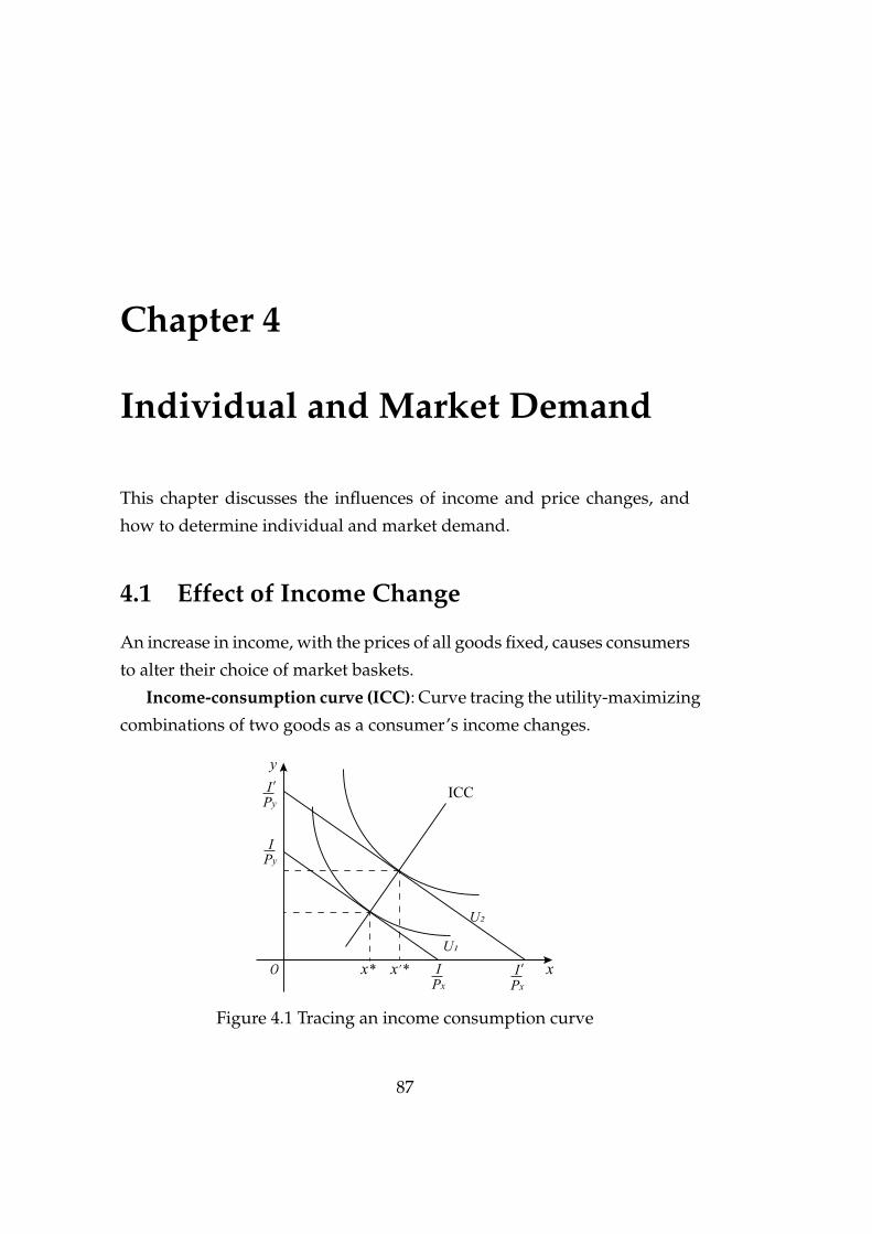
Chapter 4
Individual and Market Demand
This chapter discusses the influences of income and price changes, and
how to determine individual and market demand.
4.1 Effect of Income Change
An increase in income, with the prices of all goods fixed, causes consumers
to alter their choice of market baskets.
Income-consumption curve (ICC): Curve tracing the utility-maximizing
combinations of two goods as a consumer’s income changes.
xO
U
U!
x’*
y
x*
IPy
Px
I Py
’
I Px
I ’
ICC
Figure 4.1 Tracing an income consumption curve
87

88 CHAPTER 4. INDIVIDUAL AND MARKET DEMAND
Thus, at each point along a price consumption curve, utility is maxi-
mized, and all income is spent.
To find an income consumption curve, we change I , leaving prices
fixed. As shown in Figure 4.1, the demand of both x and y rises when
income rises.
Normal good: An increase in a person’s income can lead to more con-
sumption of the good being purchased, then its demand will increase
when px and py are fixed.
Most goods are normal goods, especially when income is low.
Inferior good: An increase in income can lead to less consumption of
one of the two goods being purchased when px and py are fixed.
As income continuously increases, more and more goods become to be
inferior goods such as potato, low quality goods, etc.
xO
U U!
y
x*
IPy
Px
I Py
’
I
Px
I ’
ICC
x’*
y*
y’*
Figure 4.2 Income consumption curve with an inferior good
As shown in Figure 4.2, we have I ′ > I , x′∗ > x∗, and y′∗ < y∗. So, x
is normal good and y is inferior good. This curve illustrates that, for all

4.1. EFFECT OF INCOME CHANGE 89
income levels, only x is normal. Notice that if there are only two goods in
the economy, they cannot be inferior goods at the same time.
Engel curves: Curve relating the quantity of a good consumed to in-
come.
In the left diagram in Figure 4.3, food is a normal good and the Engel
curve is upward sloping.
30
20
10
04 8 12 16
Engel Curve
Income
(dollars per
month)
Food (units
per month)
30
20
10
05 10
Income
(dollars per
month)
Hamburger (units
per month)
Inferior
Normal
Figure 4.3 Engel cures
In the right diagram in Figure 4.3, however, hamburger is a normal
good for income less than $18 per month and an inferior good for income
greater than $18 per month. That is,the income-consumption curve has
a positive slope for low incomes, then it takes a zero slope for a higher
income, and then it takes a negative slope for even higher incomes.
Expenditures Less than 10,000- 20,000- 30,000- 40,000- 50,000- 70,000 and19,999 29,999 39,999 49,999 59,999 69,999 above
Entertainment 1,038 1,165 1,407 1,969 2,131 2,548 4,655Owned Dwelling 1,770 2,134 2,795 3,581 4,198 5,566 11,606Rented Dwelling 3,919 3,657 4,054 3,878 4,273 3,812 3,072
Health Care 1,434 2,319 3,124 3,539 3,709 4,702 6,417Food 3,466 3,706 4,432 5,194 5,936 6,486 10,116
Clothing 798 766 960 1,321 1,518 1,602 2,928
Table 4.1: Annual U.S. Household Consumer Expenditures

90 CHAPTER 4. INDIVIDUAL AND MARKET DEMAND
Example 4.1 (Consumer Expenditures in the United States) We can derive
Engel curves for groups of consumers. This information is particularly
useful if we want to see how consumer spending varies among different
income groups.
From Table 4.1, one can see that health care and entertainment are nor-
mal goods, as expenditures increase with income. Rental housing, howev-
er, is an inferior good for incomes above $40,000.
The Supplemental Nutrition Assistance Program (SNAP)
The Supplemental Nutrition Assistance Program (SNAP), formerly known
as the Food Stamp Program, is a federal program that provides food-
purchasing assistance for low- and no-income people. If people only have
SNAP funds, they can’t withdraw cash or use their cards to pay for hous-
ing or non-food items.
Other
goods
Food
$100=A
z
(8)(10)
1F
$5
1F
$5
$85=A
$60=A!
$150=A’’
U1
U2
W
W ’
A’
Y
F! FG
F z’
(13) (20) (30)
Figure 4.4 Evaluating SNAP using consumer theory

4.1. EFFECT OF INCOME CHANGE 91
Consumer theory can be used to evaluate this program. We show this
by considering a specific example in which a consumer receives $50 worth
of SNAP funds a week. We assume the consumer has a weekly income of
$100 and the price of food is pf = $5 per unit.
The pre-subsidy budget line is AZ. The SNAP subsidy shifts the bud-
get line to AA′Z ′. Over the AA′ range, the budget line is horizontal since
the $50 in free good SNAP funds permits the recipient to purchase up to
10 units of good while leaving his or her entire income of $100 to be spent
on other goods. Over 10 units of food, the consumer has to pay for it by $5
per unit. Thus, the A′Z ′ portion of the budget line has a slope of −5. Note
that this new budget line is not straight line, but has a kink at A′.
The SNAP funds will affect the recipient in one of two ways. Figure
4.4 shows a possibility. If the consumer spends more than $50 on food, the
equilibrium, W ′, occurs on the A′Z ′ portion of the budget line. The con-
sequences of the SNAP funds are exactly the same as when the consumer
receives a cash grant of $50, leading to the budget line A′′Z.
Other
goods
Food
$100=A
z
(5)(8)
1F
$5
1F
$5
$75=A
$150=A’’
U1
U2
W
A’
Y
F FGF! z’
(10) (20) (30)
U3
Figure 4.5 Another illustration of the effect of SNAP
Figure 4.5 shows another possible outcome of the SNAP subsidy. With

92 CHAPTER 4. INDIVIDUAL AND MARKET DEMAND
a direct cash grant of $50, the consumer would be better off on the indif-
ference curve U3, which is prohibited by the SNAP funds. The consumer
has to choose among the options on the AA′Z ′ budget line, and thus the
best choice is the kink point A′. Therefore, the consumer would be better
off if the subsidy is given as cash instead of as the SNAP funds.
In summary, in the first case, the consumer is equally well off under
either cash grants or SNAP funds; in the second case, the consumer would
be better off under cash grants. There is no such a case, however, where
the consumer is better off with SNAP funds.
The same arguments and figures could be used to discuss a college
trust fund. When given a college trust fund that must be spent on educa-
tion, the student moves from W to A′, a corner solution. If, however, the
trust fund could be spent on other consumption as well as education, the
student would be better off on the indifference curve U3.
4.2 Derivation of the Demand Curve from Utili-
ty Maximization
There are two approaches to derive the demand curve of a consumption
good from utility maximization.
1. Graphical derivation
To find the demand for x, we change px, while holding py and I constant.
Let px > px′ > px
′′. We can get the baskets that maximize utility for
these prices and have other optimal baskets in a similar way. Connecting
these points smoothly, we can get the price-consumption curve depicted
in the upper diagram of the Figure 4.6.
The lower diagram in Figure 4.6 gives the demand curve, which relates
the price of the good to the quantity demanded Thus, demand for x is a
function of px, py and I .

4.2. DERIVATION OF THE DEMAND CURVE FROM UTILITY MAXIMIZATION93
xO
y
IPy
Px
I Px
I
’ Px
I
’’
xO
P
Px
Px’’
x’*x*
Px’
x’’*
D
price-consumption
curve
Figure 4.6 Deriving demand curve from utility maximization
2. Algebraic derivation
Use the two conditions for utility maximization:
MRS = px
py
, (4.1)
and
pxx + pyy = I. (4.2)
Solving equation (4.1) and (4.2), we can find x∗ and y∗ as functions of px,
py and I . Let illustrate with the following example.
Example 4.2 Suppose that preferences are represented by Cobb-Douglas

94 CHAPTER 4. INDIVIDUAL AND MARKET DEMAND
utility function
U(x, y) = x13 y
23 .
Then,
MRS = y
2x.
Equalizing MRS and px
py, we have
y
2x= px
py
,
and then
y = 2xpx
py
.
Substituting y = 2xpx
pyinto the budget line, we have
pxx + py(2xpx
py
) = I
or
3pxx = I.
Therefore, we obtain
x∗ = I
3px
= Dx.
Let I = 50 and py = 2. Then x∗ = 503px
.
To derive the demand curve, consider the following numerical illustra-
tion:
• px = 1 ⇒ x = 503 = 16.6,
• px = 5 ⇒ x = 5015 = 10
3 = 3.3,
• px = 10 ⇒ x = 5030 = 5
3 = 1.6.
Connecting these points and other points obtained in a similar way s-
moothly, we can have an indifference depicted in Figure 4.7.
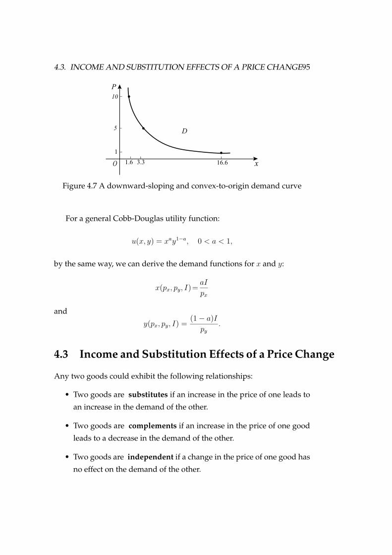
4.3. INCOME AND SUBSTITUTION EFFECTS OF A PRICE CHANGE95
xO
P
D
10
5
1
1.6 3.3 16.6
Figure 4.7 A downward-sloping and convex-to-origin demand curve
For a general Cobb-Douglas utility function:
u(x, y) = xay1−a, 0 < a < 1,
by the same way, we can derive the demand functions for x and y:
x(px, py, I)= aI
px
and
y(px, py, I) = (1 − a)Ipy
.
4.3 Income and Substitution Effects of a Price Change
Any two goods could exhibit the following relationships:
• Two goods are substitutes if an increase in the price of one leads to
an increase in the demand of the other.
• Two goods are complements if an increase in the price of one good
leads to a decrease in the demand of the other.
• Two goods are independent if a change in the price of one good has
no effect on the demand of the other.

96 CHAPTER 4. INDIVIDUAL AND MARKET DEMAND
The fact that goods can be complements or substitutes suggests that
when studying the effects of price changes in one market, it may be im-
portant to look at the consequences in related markets.
• Substitution effect: Change in consumption of a good associated
with a change in its price, with the level of utility held constant.
Say, when the price of a good falls, consumers will tend to buy more
of the good that has become cheaper and less of those goods that
are now relatively more expensive. This response to a change in the
relative prices of goods is the substitution effect.
• Income effect: Change in consumption of a good resulting from a
change in purchasing power, with prices held constant.
Say, when the price of a good falls, because one of the goods is
now cheaper, consumers enjoy an increase in real purchasing power.
The change in demand resulting from this change in real purchasing
power is the income effect.
The total effect of a change in price is given theoretically by the sum of
the substitution effect and the income effect:
Total effect = substitution effect + income effect
Income and Substitute Effects: Normal Good
The consumer is initially at A on budget line RS. With a decrease in the
price of food, the consumer moves to B on the new budget line RT and
U2. When the price of food falls, consumption increases by F1F2 as the
consumer moves to B. The resulting change in food purchased can be
broken down into substitution and income effects.

4.3. INCOME AND SUBSTITUTION EFFECTS OF A PRICE CHANGE97
Figure 4.8 Income and substitution effects: normal good
Since the real purchasing power increases due to the price decrease,
to find the substitution effect, the consumer should spend less income in
order to keep the same utility level as U1. Note that any parallel line of RT
has the same slope.
Thus, the way to determine the substitution effect (and consequently
income effect) is simply as follows:
Draw a parallel line of the new budget line RT , which is tan-
gent to the initial indifference curve U1.
We can do by shifting the new budget line RT parallely toward the initial
indifference curve U1 and stopping at the tangent point D of U1. Thus,
moving from A to D represents the effect of the decrease in the food price
on food consumption, which is F1E, while maintaining the same level of
satisfaction. This is the substitution effect.
The remaining change, from B to D, is the income effect. The differ-
ence between the new budget line RT and its parallel budget line repre-
sents the effect of the increase in real purchasing power on food consump-
tion, which is EF2, resulting in the increase in utility from U1 to U2.

98 CHAPTER 4. INDIVIDUAL AND MARKET DEMAND
Because food is a normal good, the income effect EF2 is positive, hence
their income and substitute effects move in the same direction as shown
by the arrows in Figure 4.8.
Also, note that there is no income effect when an indifference curve is
perfect substitutes and there is no substitution effect when an indifference
is perfect complements.
Income and Substitute Effects: Inferior Good
The consumer is initially at A on budget line RS. With a decrease in the
price of food, the consumer moves to B. Again, the resulting change in
food purchased can be broken down into a substitution effect, F1E (as-
sociated with a move from A to D), and an income effect, EF2 (associated
with a move from D to B). In this case, food is an inferior good because the
income effect is negative. However, because the substitution effect exceed-
s the income effect, the decrease in the price of food leads to an increase in
the quantity of food demanded.
Figure 4.9 Income and substitution effects: inferior good

4.3. INCOME AND SUBSTITUTION EFFECTS OF A PRICE CHANGE99
Thus, when a good is an inferior good, the income effect is negative,
hence their income and substitute effects move in the opposite directions
as shown by the arrows in Figure 4.9.
Income and Substitute Effects: Giffen Good
So far, the demand curves we derived are all downward-sloping, that is,
demand for x will decrease as its price increases. However, it is possible
for a consumer to have indifference curves so that the law of demand does
not hold for some good.
A good is said to be a Giffen good if the quantity demanded will fall
when its price falls.
What kind of goods can be Giffen goods? The Giffen good is rarely of
practical interest because it requires a large negative income effect. But, in
practice, the income effect is usually small.
As shown in Figure 4.10, a lower price could lead to less consumption.
The consumer purchases less of food when its price falls. Note that the
indifference curves that produce this result are downward-sloping, non-
intersecting, and convex; that is, they do not contradict any of the basic
assumptions about preferences.
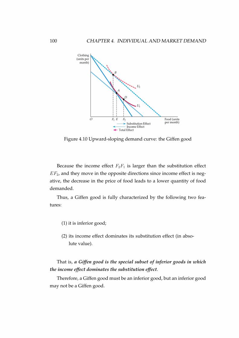
100 CHAPTER 4. INDIVIDUAL AND MARKET DEMAND
Figure 4.10 Upward-sloping demand curve: the Giffen good
Because the income effect F2F1 is larger than the substitution effect
EF2, and they move in the opposite directions since income effect is neg-
ative, the decrease in the price of food leads to a lower quantity of food
demanded.
Thus, a Giffen good is fully characterized by the following two fea-
tures:
(1) it is inferior good;
(2) its income effect dominates its substitution effect (in abso-
lute value).
That is, a Giffen good is the special subset of inferior goods in which
the income effect dominates the substitution effect.
Therefore, a Giffen good must be an inferior good, but an inferior good
may not be a Giffen good.

4.4. FROM INDIVIDUAL TO MARKET DEMAND 101
4.4 From Individual to Market Demand
We have derived the demand curve for an individual consumer. To obtain
a market demand curve, we simply add all individual demands at given
prices. Two points should be noted:
(1) The market demand curve will shift to the right as more
consumers enter the market.
(2) Factors that influence the demands of many consumers will
also affect market demand.
The aggregation of individual demands into market becomes impor-
tant in practice when market demands are built up from the demands of
different demographic groups or from consumers located in different ar-
eas.
Example 4.3 Consider the numerical example with two consumers. Mak-
ing the summation of two individuals’ demand, we obtain the market de-
mand as shown in Table 4.3 and Figure 4.11.
px for good x DAx for A DB
x for B Market demand Dx
$1 10 12 22$2 7 5 12$3 3 1 4
Table 4.2: Determining the market of demand curve

102 CHAPTER 4. INDIVIDUAL AND MARKET DEMAND
xO
Px
1
2
3
A
Dx
B
Dx Dx for market
Figure 4.11 From individual demand to market demand
4.5 Consumer Surplus
Consumers purchase goods and services because they are better off from
doing so; otherwise, the purchase would not take place. The term con-
sumer surplus refers to the net benefit, or gain.
Consumer surplus: Difference between what a consumer is willing to
pay for a good and the amount actually paid.
To obtain the measure of consumer surplus associated with purchasing
a certain amount of a good or service, we may ask the question: What is
the maximum amount you would be willing to pay, that is, what is the
maximum total benefit, and what is the total cost? After we have the an-
swers, the consumer surplus is defined by:
Consumer surplus = Total benefit - Total cost.
That is, consumer surplus is the difference between the willingness-to-
pay of the consumer and what the person actually has to pay for it.

4.5. CONSUMER SURPLUS 103
E
d
Q=61 2 3 4 5 7 80
P=$3
$4
$5
$6
$7
$8
Price
per cup
Cups of
espresso
per day
Figure 4.12 The discrete approach of calculating consumer surplus
To show this, let us consider a specific example. Suppose that a person
purchases 6 cups of espresso at the price p = $3. The total cost = 3×6 = 18.
Total benefit from purchasing 6 units at a price $ 3, however, is the sum of
marginal benefit (the sum of 6 units shaded rectangles of Figure 4.12), i.e.,
total benefit = $8 + $7 + $6 + $5 + $4 + $3 = 33.
Thus, the consumer surplus = total benefit − total cost = 33 − 18 = 15.
In general, with a smooth demand curve indicated in Figure 4.13, con-
sumer surplus equals the area TEP .
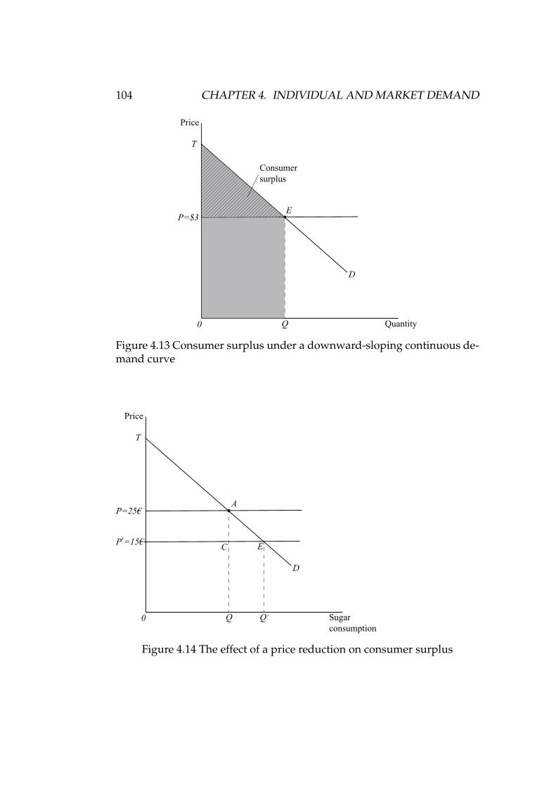
104 CHAPTER 4. INDIVIDUAL AND MARKET DEMAND
E
Q0
P=$3
Price
Quantity
D
T
Consumer
surplus
Figure 4.13 Consumer surplus under a downward-sloping continuous de-mand curve
E
Q0
P=25€
Price
Sugar
consumption
D
T
A
C
Q’
P’=15€
Figure 4.14 The effect of a price reduction on consumer surplus

4.6. NETWORK EXTERNALITIES 105
The concept of consumer surplus can also be used to identify the net
benefit of a change in the price of a commodity. In Figure 4.14, at a price
of 25 cents per unit, consumer surplus is TAP . At a price of 15 cents per
unit, consumer surplus is TEP ′. The increase in consumer surplus from
the price reduction is thus the shaded area PAEP ′, which is a measure of
the benefit to consumers of a reduction in the price from 25 to 15 cents.
Consumer surplus measures the aggregate benefit that consumers ob-
tain from buying goods in a market. When we combine consumer surplus
with the aggregate profits that producers obtain, we can evaluate both the
costs and benefits not only of alternative market structures, but of public
policies that alter the behavior of consumers and firms in those markets.
4.6 Network Externalities
Network externality: When each individual’s demand depends on the
purchases of other individuals.
Positive network externality: The quantity of a good demanded by a
typical consumer increases in response to the growth in purchases of other
consumers (e.g., telephones, emails, Facebook, Tik Tok, WeChat, etc.).
Negative network externality: The quantity demanded decreases to
the growth in purchases of other consumers (e.g., an individual has the
desire to own exclusive or unique goods).
Positive Network Externalities
Bandwagon effect: Positive network externality in which a consumer wish-
es to possess a good in part because others do, i.e., to have a good because
of the perception that almost everyone else has it.
With a positive network externality, the quantity of a good that an in-
dividual demands grows in response to the growth of purchases by other
individuals. Here, as the price of the product falls from $30 to $20, the
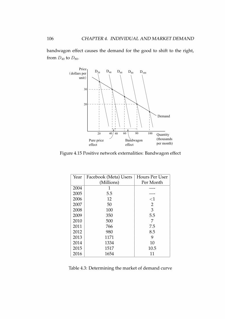
106 CHAPTER 4. INDIVIDUAL AND MARKET DEMAND
bandwagon effect causes the demand for the good to shift to the right,
from D40 to D80.
Price
(dollars per
unit)
Quantity
(thousands
per month)
Demand
30
20
20 40 48 60 80 100
Pure price
effect
Bandwagon
effect
D20 D40 D60 D80 D100
Figure 4.15 Positive network externalities: Bandwagon effect
Year Facebook (Meta) Users Hours Per User(Millions) Per Month
2004 1 —-2005 5.5 —-2006 12 <12007 50 22008 100 32009 350 5.52010 500 72011 766 7.52012 980 8.52013 1171 92014 1334 102015 1517 10.52016 1654 11
Table 4.3: Determining the market of demand curve

4.6. NETWORK EXTERNALITIES 107
Positive network externalities have been crucial drivers for many mod-
ern technologies over many years.
Example 4.4 (Facebook (Meta)) By early 2011, with over 700 million user-
s, Meta previously known as Facebook became the world’s second most
visited website (after Google). By 2021, there are about 2 billion users. A
strong positive network externality was central to Facebook’s success.
Negative Network Externalities
Snob effect: Negative network externality in which a consumer wishes to
own an exclusive or unique good.
The quantity demanded of a “snob” good is higher when the fewer is
the number of people who own it (e.g., garments specially designed by
a well-known fashion designer, special designs of watches, automobiles,
buildings, etc.).
Price
(dollars per
unit)
Quantity
(thousands
per month)
30,000
15,000
2 4 8 14
Pure Price Effect
Net Effect
D8
D4D6
D2
6
Demand
Snob Effect
Figure 4.16 Negative network externalities: Snob effect

108 CHAPTER 4. INDIVIDUAL AND MARKET DEMAND
The snob effect is a negative network externality in which the quantity
of a good that an individual demands falls in response to the growth of
purchases by other individuals.
Here, as the price falls from $30,000 to $15,000 and more people buy
the good, the snob effect causes the demand for the good to shift to the
left, from D2 to D6.

Part III
Supply Side of Market
109


111
Part 2 presents the theoretical core of production and competitive fir-
m’s supply and market supply.

112

Chapter 6
Theory of Production
In this chapter and the next we discuss the theory of the firm, which de-
scribes how inputs (such as labor, capital, and raw materials) can be trans-
formed into outputs and how a firm makes cost-minimizing production
decisions and how the firm’s resulting cost varies with its output.
6.1 The Technology of Production
Firm: any organization that engages in production.
The production decisions of firms can be understood in three steps:
1. Production Technology: How inputs (such as labor, capital,
and raw materials) can be transformed into outputs.
2. Cost Constraints: What possible combinations of inputs can
be used with a given expenditure on production.
3. Input Choices: Just as a consumer is constrained by a limited
budget, the firm is concerned about the cost of production
and the prices of labor, capital, and other inputs.
We can divide inputs into the broad categories of labor, materials and
capital, each of which might include more narrow subdivisions.
113

114 CHAPTER 6. THEORY OF PRODUCTION
• Labor inputs include skilled workers (financial analyst, carpenter-
s, engineers) and unskilled workers (cleaners, manual workers), as
well as the entrepreneurial efforts of the firm’s managers.
• Materials include steel, plastics, electricity, water, and any other good-
s that the firm buys and transforms into final products.
• Capital includes land, buildings, machinery and other equipment,
as well as inventories.
Production Function: A relationship between inputs and outputs that i-
dentifies the maximum output produced by a firm for every combination
of inputs with a given technology.
A production is technologically efficient if the maximum quantity of a
commodity can be produced by each specific combination of inputs. Thus,
production specified by production function is technologically efficient. If
a firm is rational, it should always operate in a technologically efficient
way to produce outputs.
We can present a production function in tabular, graphical, or mathe-
matical form.
For example, in mathematical form, we have
q = F (K, L),
where q is the number of units of output, K the number of units of capital
input, L the number of units of labor input, and F is production function.
A commonly used production is the so-called Cobb-Douglas produc-
tion function:
F (K, L) = AKαLβ.
Suppose that α = β = 12 and A = 1. We have
q = K12 L
12 .

6.2. PRODUCTION IN SHORT-RUN 115
Then, for a particular combination of inputs, say, K = 16 and L = 36, the
maximum output obtainable with this technology is
q = (16)12 (36)
12 = 4 × 6 = 24.
6.2 Production in Short-Run
We first define the relevant concepts as follows.
Short run: A period of time in which changing the employment levels
of some inputs is impractical, i.e., it is a time period in which at least one
input is fixed.
Fixed inputs: Production factors that cannot be varied over the time
period involved.
Long run: A period of time in which the firm can vary all its inputs.
For example, for a factory, short run is long enough to hire an extra
worker but is not long enough to build an extra production line.
6.2.1 Various Product Curves in Short Run
Assume there are two factors of production: labor (L) and capital (K).
In the short run we usually assume K is fixed and L is a variable input.
Given fixed K, the firm can vary L to produce different amounts of output.
• Total Product (TP): total output produced;
• Average Product (AP): Output per unit of a variable factor. That is,
AP = total product/variable factor.
For example, average product of labor is given by
APL = TP
L.
• Marginal Product (MP): the change in output resulting from a change
in the amount of the input, holding the quantities of other inputs

116 CHAPTER 6. THEORY OF PRODUCTION
constant. For example, marginal product of labor:
MPL = ∆TP/∆L.
The Average-Marginal Products Relationship
• If MPL > APL, then APL must rise.
• If MPL < APL, then APL must fall.
• If MPL = APL, then APL reaches its maximum.
Note that if MPL is constant, APL is identical to MPL, hence constant in L.
Example 6.1 Suppose q = F (K, L) = 10KL2. Then APL = qL
= 10KL and
MPL = ∂q/∂L = 20KL. We verify that MPL > APL implies APL increases.
Example 6.2 (Production with One Variable Input (Labor)) Consider the
numerical example depicted in Table 6.1.
Fixed amount Amount Total product Average product Marginal product
of land of labor (L) (TPL) of labor (APL) of labor (MPL)
5 0 0 −− −−5 1 50 50 50
5 2 150 75 100
5 3 300 100 150
5 4 400 100 100
5 5 480 96 80
5 6 540 90 60
5 7 580 83 40
5 8 610 76 30
5 9 610 68 0
5 10 580 58 -30
Table 6.1: Production with one variable input (labor)

6.2. PRODUCTION IN SHORT-RUN 117
q
L3 6 9
300
400
q
50
100
TP
150
AP
output
per L
L
MPL
Figure 6.1 The relationship between TP, MP and AP
The total output curve in the upper diagram in Figure 6.1 shows the
output produced for different amounts of labor input.
The average and marginal products in the lower diagram in Figure 6.1
can be obtained (using the data in Table 6.1) from the total product curve.
With 3 units of labor, the marginal product is 150 because the tangent
to the total product curve has a slope of 150. The average product of la-
bor, however, is 100, and then the average product of labor continue to
increase. With 4 units of labor, the marginal product of labor and the aver-
age product of labor are interest, the average product of labor reaches its
maximum at this point.
When the labor input is 5 units, the marginal product is below the av-
erage product, so the average product is falling. Once the labor input ex-

118 CHAPTER 6. THEORY OF PRODUCTION
ceeds 9 units, the marginal product becomes negative, so that total output
falls as more labor is added. When total output is maximized, the slope
of the tangent to the total product curve is 0, as is the marginal product.
Beyond that point, the marginal product becomes negative.
6.2.2 The Geometry of Production Curves
(1) Average product: APL = T PL
= qL
.
Note that the slope of any line from the origin to a point on the TP
curve has slope = ∆q∆L
= q−0L−0 = q
L. That is, APL is the slope of the line
which connects the origin to the TP curve. At point C in Figure 6.3, APL
reaches a maximum since the ray OC is the steepest ray from the origin
that still touches the TP curve.
L
Q
l
q
TPC
B
Figure 6.2 The geometry of production curves
(2) Marginal product: MPL = ∆T P∆L
= ∆q∆L
.
That is, MPL is the slope of the TP curve. The following law of dimin-
ishing marginal product (DMP) reveals the shape of the TP curve. MPL
increases to a point and then decreases. This is, the slope of TP first in-
creases and then eventually starts to decrease. When MPL = 0, the TP
curve reaches its maximum.

6.2. PRODUCTION IN SHORT-RUN 119
6.2.3 The Law of Diminishing Marginal Returns
The law of diminishing (marginal) returns (DMR): As the amount of a
variable input increases with a fixed amount of other inputs and fixed
technology, a point is reached beyond which the marginal product of the
variable input begins to fall.
That is, the marginal product of a variable input eventually decreases
with a given technology and other inputs fixed.
Example 6.3 Farm adds fertilizer (variable) to an acre of land (fixed); and
the numerical example as follows:
K,L q MPL Diminishing Returns
1,0 0 –
1,1 10 10
1,2 30 20 ↓1,3 40 10 ↓1,4 45 5 ↓1,5 48 3 ↓
Table 6.2: Production with one variable input (labor)
Remarks on DMR
(1) Technology Improvement. Labor productivity (output per unit of la-
bor for an economy or industry as a whole) can increase if there are im-
provements in technology, even though any given production process ex-
hibits diminishing returns to labor. The law of diminishing marginal re-
turns was central to the thinking of political economist Thomas Malthus
(1766-1834). Malthus predicted that as both the marginal and average pro-
ductivity of labor fell and there were more mouths to feed, mass hunger
and starvation would result. Malthus was wrong (although he was right
about the diminishing marginal returns to labor). Over the past century,

120 CHAPTER 6. THEORY OF PRODUCTION
technological improvements have dramatically altered food production in
most countries (including developing countries, such as India). As a re-
sult, the average product of labor and total food output have increased.
Hunger remains a severe problem in some areas, in part because of the
low productivity of labor there.
(2) Changes in other inputs. Even though both labor and capital are
variable in the long run, it is useful for a firm that is choosing the optimal
mix of inputs to ask what happens to output as each input is increased,
with the other input held fixed. Because adding one factor while holding
the other factor constant eventually leads to lower and lower incremental
output, the isoquant must become steeper as more capital is added in place
of labor and flatter when labor is added in place of capital. There are also
diminishing marginal returns to capital. With labor fixed, the marginal
product of capital decreases as capital is increased.
Year Index of World Food Production Per Cap
1961-64 100
1965 101
1970 105
1975 106
1980 109
1985 115
1990 117
1995 119
2000 127
2005 135
2010 146
2013 151
Table 6.3: Index of world food production per cap.
Example 6.4 (Malthus and The Food Crisis) Table 6.3 shows that techno-

6.2. PRODUCTION IN SHORT-RUN 121
logical improvements have dramatically altered food production.
6.2.4 Labor Productivity and the Standard of Living
Consumers in the aggregate can increase their rate of consumption in the
long run only by increasing the total amount they produce. Understand-
ing the causes of productivity growth is an important area of research in
economics.
Development of new technologies allowing factors of production to be
used more effectively.
Example 6.5 (Labor Productivity and the Standard of Living) Will the s-
tandard of living in the United States, Europe, and Japan continue to im-
prove, or will these economies barely keep future generations from being
worse off than they are today?
Because the real incomes of consumers in these countries increase only
as fast as productivity does, the answer depends on the labor productivity
of workers.
United States Japan France Germany UK
GDP
Per Hour $62.41 $39.39 $60.28 $58.92 $47.39
Years Labor (%) Labor (%) Labor (%) Labor (%) Labor (%)
Productivity Productivity Productivity Productivity Productivity
1970-1979 1.7 4.5 4.3 4.1 3.2
1980-1989 1.4 3.8 2.9 2.1 2.2
1990-1999 1.7 2.4 2.0 2.3 2.3
2000-2009 2.1 1.3 1.2 1.1 1.5
2010-2014 0.7 1.2 0.9 1.2 0.5
Table 6.4: Annual rate of growth of labor productivity (in 2010 U.S dollars)in developed countries

122 CHAPTER 6. THEORY OF PRODUCTION
6.3 Production in the Long-Run
Now we return to the case of long-run and assume that labor and capi-
tal both are variable, and introduce the important concept of isoquant in
production decision.
6.3.1 Production Isoquants
Production Isoquant: A curve that shows all the combinations of inputs
that, when used in a technologically efficient way, yield the same total
output.
Isoquants show the input flexibility that firms have when making pro-
duction decisions: They can usually obtain a particular output by substi-
tuting one input for another. It is important for managers to understand
the nature of this flexibility.
K
L
q=2
q=3
1 2 3 4
4
3
2
1
Figure 6.3 A set of production isoquants or an isoquant map
For example, if q = K12 L
12 , the isoquant for q = 2 must include the

6.3. PRODUCTION IN THE LONG-RUN 123
following pair of inputs:
K = 1, L = 4;
K = 2, L = 2;
K = 3, L = 43
;
K = 4, L = 1.
Isoquants are very similar to indifference curves in their characteristic-
s. By analogous reasoning, we can explain several characteristics of iso-
quants.
i) Isoquant slopes downward. If we increase the quantity of
one input employed and keep output unchanged, then we
must reduce the amount of the other inputs.
ii) Isoquants can never intersect.
iii) Lying further to the northeast identify higher levels of out-
puts.
iv) Isoquants are generally convex to the origin.
6.3.2 Marginal Rate of Technical Substitution
The slope of an isoquant measures the marginal rate of technical Substitu-
tion between the inputs.
Marginal rate of technical substitution (MRTS): The rate at which one
input can be substituted for another with output remaining constant.
By the same reasoning as indifference curves, the marginal rate of tech-
nical substitution is equal the absolute value of the slope of an isoquant,
i.e.,
MRTSLK =∣∣∣∣∣∆K
∆L
∣∣∣∣∣ .

124 CHAPTER 6. THEORY OF PRODUCTION
Also, it is equal to the ratio of the marginal products of the inputs, i.e.,
MRTSLK = MPL
MPK
.
An isoquants is strictly convex implies the marginal rate of technical
substitution diminishes, known as the diminishing marginal rate of tech-
nical substitution.
Limiting Isoquants:
• Perfect substitutes: The rate at which capital and labor can be sub-
stituted for each other is the same no matter what level of inputs is
being used.
That is, isoquants are straight lines so that the MRTS is constant. It is
also called a linear production function, which can be written as
q = F (K, L) = aK + bL.
L
K
Q=8
Q=10
Figure 6.4 Perfect substitutes production function

6.3. PRODUCTION IN THE LONG-RUN 125
• Perfect complement: Indicate that capital and labor cannot be sub-
stituted for each other in production.
It is sometimes called the (fixed-proportions production function)
or a Leonitief production function, which can be written as
q = F (K, L) = min{aK, bL}.
L
K
q=8
q=10
Figure 6.5 Production function with L-shaped isoquants
The isoquants for these two production functions are convex, but not
strictly convex.
6.3.3 Returns to Scale
A fire can increase its output by increasing all inputs. We then want to
know the scale of return.
Returns to scale: Effect on output of equal proportionate change in all
inputs.
E.g., double inputs ⇒ what will happen to output?
There are three types of production processes:

126 CHAPTER 6. THEORY OF PRODUCTION
• Constant returns to scale (CRS): output doubles when all inputs are
doubled;
• Increasing returns to scale (IRS): output more than doubles when all
inputs are doubled;
• Decreasing returns to scale (DRS): output less than doubles when
all inputs are doubled.
Graphically, the three types of returns to scale are illustrated in Figure
6.6.
L
K
q=10
q=20
1
1
2
2
L
K
q=10
q=18
1
1
2
2
L
K
q=10
q=22
1
1
2
2
(a) CRS (b) DRS (c) IRS
Figure 6.6 Three types of returns to scale
Returns to scale can be checked in the following way if a production
function is a homogeneous function, i.e.,
F (λK, λL) = λtF (K, L), λ > 0.
• if the exponent of λ, t < 1, F (K, L) displays DRS,
• if the exponent of λ, t = 1, F (K, L) displays CRS,
• if the exponent of λ, t > 1, F (K, L) displays IRS.
Example 6.6 Suppose
F (K, L) = 5K13 L
23 .

6.3. PRODUCTION IN THE LONG-RUN 127
Then
F (λK, λL) = 5(λK)13 (λL)
23 = 5λ
13 + 2
3 K13 L
23 = 5λK
13 L
23 = λF (K, L).
Since the exponent of λ is 1, it is CRS.
Example 6.7 Suppose
F (K, L) = KL.
Then
F (λK, λL) = (λK)(λL) = λ2KL = λ2F (K, L).
Since the exponent of λ is 2, it is IRS.
For a general Cobb-Douglas production
F (K, L) = KαLβ α > 0, β > 0,
we have
F (λK, λL) = (λK)α(λL)β = λα+βKαLβ = λα+βF (K, L).
Therefore, we have
• if the exponent (α + β) < 1, F (K, L) displays DRS,
• if the exponent (α + β) = 1, F (K, L) displays CRS,
• if the exponent (α + β) > 1, F (K, L) displays IRS.
Example 6.8 Suppose
F (K, L) = aK + bL.
Then
F (λK, λL) = a(λK) + b(λL) = λ(aK + bL) = λF (K, L).
Since the exponent of λ is 1, it is CRS. Thus, any linear production function
is CRS.

128 CHAPTER 6. THEORY OF PRODUCTION
Example 6.9 Suppose the production is given by a fixed-proportion pro-
duction function
q = F (K, L) = min{aK, bL}.
Then
F (λK, λL) = min{λaK, λbL} = λ min{aK, bL} = λF (K, L).
Since the exponent of λ is 1, it is CRS. Thus, any fixed proportional pro-
duction function is CRS.
Remarks: Returns to scale need not be uniform across all possible lev-
els of output. As a general rule, increasing returns to scale are likely to be
the case when the scale of operations is small, perhaps followed by an in-
termediate range when constant returns prevail, with decreasing returns
to scale becoming more relevant for large-scale operations. In other words,
a production function could embody increasing, constant, and decreasing
returns to scale at different levels of output.

Chapter 7
The Cost of Production
We now discuss various types of production cost and analyze the relation-
ship between cost of production and output of production.
7.1 The Nature of Cost
In analyzing production decision of a firm, the basic concept is the eco-
nomic costs of production.
Economic costs: The sum of explicit and implicit costs.
Explicit costs (i.e.,accounting cost): the payments made for resources
which the firm purchases or hires from outside sources (such as wages,
interest paid on debt, and land rent).
Implicit costs: the costs of resources which the firm uses but neither
buys nor hires from outside sources.
—- Provided these resources have an alternative use, there is a cost
involved although no explicit monetary payment is made. They stand for
the monetary payments the resources could earn in their best alternative
use. For example,
• If you own a building, implicit costs of running a small store include
the rent that could have been earned if the building was leased to
another firm.
129

130 CHAPTER 7. THE COST OF PRODUCTION
• Salary that could be earned by owner if employed in another busi-
ness.
• Interest that could be earned by lending money to someone else.
The sum of explicit and implicit costs may be regarded as opportunity
costs. That is, economic cost equals opportunity cost.
Opportunity cost: Cost associated with opportunities forgone when
one alternative is chosen.
—- If they are used to produce one good, they are not available for
producing other goods. For example, cost of washing machine might be a
number of refrigerators.
The concept of opportunity cost is particularly useful in situations where
alternatives that are forgone do not reflect monetary outlays.
Sunk cost: Expenditure that has been made and cannot be recovered
(i.e., no alternative use).
Because a sunk cost cannot be recovered, it should not influence the
firm’s decisions. For example, if specialized equipment for a plant cannot
be converted for alternative use, the expenditure on this equipment is a
sunk cost. Because it has no alternative use, its opportunity cost is zero.
Thus it should not be included as part of the firm’s economic costs.
A prospective sunk cost is an investment. Here the firm must decide
whether that investment in specialized equipment is economical.
7.2 Short-Run Costs of Production
7.2.1 Short-Run Total, Average, and Marginal Costs
The short-run costs of production include:
(a) Total Fixed Cost (TFC): Costs of fixed factors of production in the
short-run.

7.2. SHORT-RUN COSTS OF PRODUCTION 131
Fixed cost does not vary with the level of output — it must be paid
even if there is no output.
(a′) Average Fixed Cost (AFC):
AFC = TFC
qwhere q = output level.
(b) Total Variable Cost (TVC): Costs incurred by the firm that depend on
how much output it produces. These costs are associated with the
variable inputs.
For example, labor cost depends on the number of workers hired.
(b′) Average Variable Cost (AVC):
AV C = TV C
q.
(c) Total Cost (TC):
TC = TFC + TV C.
(c′) Average Total Cost (ATC):
ATC = TC
q.
Since TC = TFC + TV C, then
ATC = TFC + TV C
q= TFC
q+ TV C
q.
So,
ATC = AFC + AV C.
(d) Marginal Cost (MC): Increase in cost resulting from the production of
132 CHAPTER 7. THE COST OF PRODUCTION
one extra unit of output.
MC = ∆TC
∆q= ∆TFC + ∆TV C
∆q.
Thus ∆TFC = 0 because only TV C varies with q. Therefore
MC = ∆TC
∆q.
Also TV C = sum of MC. That is, because fixed cost does not change
as the firm’s level of output changes, marginal cost is equal to the
increase in variable cost or the increase in total cost that results from
an extra unit of output.
Remarks:
(1) How do we know which costs are fixed and which are vari-
able? Over a very short time horizon — say, a few months
— most costs are fixed. Over such a short period, a firm
is usually obligated to pay for contracted shipments of ma-
terials. Over a very long time horizon — say, ten years —
nearly all costs are variable. Workers and managers can be
laid off (or employment can be reduced by attrition), and
much of the machinery can be sold off or not replaced as it
becomes obsolete and is scrapped.
(2) Fixed costs versus sunk costs. Fixed costs can be avoided if
the firm shuts down or goes out of business. Sunk costs, on
the other hand, are costs that have been incurred and cannot
be recovered. Fixed costs affect the firm’s decisions looking
forward, whereas sunk costs do not. Fixed costs that are
high relative to revenue and cannot be reduced might lead a
firm to shut down—eliminating those fixed costs and earn-
ing zero profit may be better than incurring ongoing losses.

7.2. SHORT-RUN COSTS OF PRODUCTION 133
Incurring a high sunk cost might later turn out to be a bad
decision, but the expenditure is gone and cannot be recov-
ered by shutting down. A sunk cost is different and does
affect the firm’s decisions looking forward.
Example 7.1 Short-Run Cost Schedule for an Individual Firm:
q TFC TV C TC MC AFC AV C ATC
0 100 0 100 − − − − − − − − − − − −1 100 90 190 90 100 90 190
2 100 170 270 80 50 85 135
3 100 240 340 70 3312 80 1131
2
4 100 300 400 60 25 75 100
5 100 370 470 70 20 74 94
6 100 450 550 80 1623 75 912
3
7 100 540 540 90 1427 771
7 9137
8 100 650 750 110 1212 811
4 9334
9 100 780 880 130 1119 862
3 9779
10 100 930 1030 150 10 93 103
1 2 3 4 5 6 7 8 9 100
100
200
300
400
500
600
700
800
900
1000
q
$
TFC
TC
TVC
TFC}
Figure 7.1 TFC is the gap between TC and TVC

134 CHAPTER 7. THE COST OF PRODUCTION
Note that in Figure 7.1 the vertical distance between TC and TV C is
equal to TFC. Also, in Figure 7.2, the vertical distance between AV C and
ATC is AFC.
1 2 3 4 5 6 7 8 9 100
20
40
60
80
100
120
140
160
180
200
$/unit
AFC
MC
ATC
AVC
AFC
AFC
AFC!
AFC!}
}
}
}Figure 7.2 AFC is the gap between AVC and ATC
If we have a specific cost function, we can easily find the related various
cost curves.
Example 7.2 Suppose that TC = 10 + 2q + 5q2. Then, we have:
TFC = 10, TV C = 2q + 5q2, AC = 10/q2 + 5q,
AFC = 10/q, AV C = 2 + 5q, MC = 2 + 10q.
7.2.2 The Shapes of Short-Run Cost Curves
Now let us examine what shapes the short-run cost curves have. We will
show that all short-run cost curves have the same shapes as the shapes
implied by the data in the previous example.

7.2. SHORT-RUN COSTS OF PRODUCTION 135
q
$
TFC
TC
TVC
TFC}
Figure 7.3 TFC is the gap between TC and TVC
$/unit
AFC
MC
ATC
AVC
AFC
AFC
AFC!
AFC!}
}
}
}q
Figure 7.4 MC curve cuts curves of AVC and ATC at their respective min-imum
The same as the product curves, we have:
(1) The average total cost of a given level of output is the slope
of the line from the origin to the total cost curve at that
level of output.

136 CHAPTER 7. THE COST OF PRODUCTION
(2) The marginal cost of a given level of output is the slope of
the line that is tangent to the total cost curve at that level
of output.
The U-shaped Marginal Cost Curve
The marginal cost curve is generally U-shaped: With the cost of additional
units of output first falling, reaching a minimum, and then rising.
The U-shape of the marginal cost curve is attributable to the law of
diminishing marginal returns.
To see why, recall the MC is defined as
MC = ∆TV C
∆q.
We know TV C = wL where w is the wage rate and L is the amount of the
variable input (labor). Thus ∆TV C = w∆L, yielding
MC = ∆TV C
∆q= w∆L
∆q= w/
∆q
∆L= w/MPL.
Thus MC and MPL have a reverse relationship. Because of the law
of diminishing marginal returns, MPL varies with the amount of output
and therefore, so must MC. At low levels of output MPL is rising; so,
correspondingly, MC(= w/MPL) must be falling. When MPL reaches a
maximum, then MC must be at a minimum. After that MPL falls, and
then MC must rise. That is, MPL rises and then falls; and correspondingly
MC will first fall and then rise.
The average variable curve (AV C) must be also U-shaped due to the
law of diminishing marginal returns. Recall AV C is defined as
AV C = TV C
q= wL
q= w/
q
L= w/APL.
In the previous chapter we saw that the law of diminishing marginal re-

7.3. LONG-RUN COSTS OF PRODUCTION 137
turns leads to an APL shaped like an inverted U. That is, APL rises, reaches
a maximum, and then falls. As a result, w/MPL (MC) must be U-shaped,
i.e., MC will fall, reach a minimum, and then rise. Thus, MC cuts AV C
and ATC at their respective minimum.
The Average-Marginal Costs Relationship
• If MC < AV C (MC < AC), the AV C (AC) must be falling.
• If MC > AV C (MC > AC), the AV C (AC) must be rising.
• If MC = AV C (MC = AC), the AV C (AC) must be at the minimum.
Again, when MC is constant, AV C is identical to MC.
Knowledge of short-run costs is particularly important for firms that
operate in an environment in which demand conditions fluctuate consid-
erably. If the firm is currently producing at a level of output at which
marginal cost is sharply increasing, and if demand may increase in the
future, management might want to expand production capacity to avoid
higher costs.
7.3 Long-Run Costs of Production
In the long run:
(a) Firms can enter or exit from an industry (will be discussed
later);
(b) A firm can vary all inputs, and thus
• the law of diminishing marginal returns does not ap-
ply;
• all costs are variable so there is no distinction between
fixed and variable costs. The remaining types of cost
are TC, ATC, and MC.

138 CHAPTER 7. THE COST OF PRODUCTION
7.3.1 Isocost Line
Isocost line: Graph showing all possible combinations of labor and capital
that can be purchased for a given total cost and given prices of inputs as
depicted in Figure 7.5. (Compare it with the budget line.)
K
Isocost line
c
w
wr
_
c
r
L
Figure 7.5 An isocost line with two inputs
To see what an isocost line looks like, recall that the total cost of pro-
ducing any particular output is given by the sum of the firm’s labor cost
wL and its capital cost rK:
C = wL + rK,
where C is total cost, w is wage rate, r is rental rate of K, and slope of the
isocost line is −wr
.
We can draw the isocost line map by varying total cost as shown in
Figure 7.6.

7.3. LONG-RUN COSTS OF PRODUCTION 139
K
Isocost varies with total
cost where c’’>c’>c
c
w
c
r
Lc
w
c
w’ ’’
c’
c’’r
r
Figure 7.6 A set of isocost lines as total cost varies
Suppose that a firm wants to produce a given level of output, q = q. We
can use the isoquant to determine the possible input combinations which
make q feasible. Which combination will be chosen?
The firm would choose whichever combination of inputs that
1) yield q units of output;
2) costs less than any other input combinations which also pro-
duce q.
7.3.2 Cost Minimization Problem
The firm wishes to find the input combination which produces a given
level of output and incurs the lowest possible costs. Thus, the firm must
find a point on the isoquant q = q which is tangent to an isocost line.
In Figure 7.7, both D and E produce q, but D costs more.
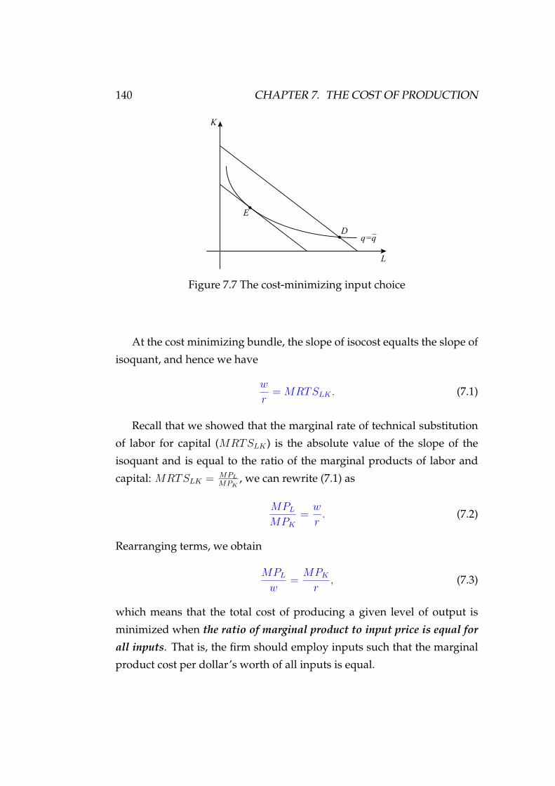
140 CHAPTER 7. THE COST OF PRODUCTION
K
L
E
Dq=q
Figure 7.7 The cost-minimizing input choice
At the cost minimizing bundle, the slope of isocost equalts the slope of
isoquant, and hence we have
w
r= MRTSLK . (7.1)
Recall that we showed that the marginal rate of technical substitution
of labor for capital (MRTSLK) is the absolute value of the slope of the
isoquant and is equal to the ratio of the marginal products of labor and
capital: MRTSLK = MPL
MPK, we can rewrite (7.1) as
MPL
MPK
= w
r. (7.2)
Rearranging terms, we obtain
MPL
w= MPK
r, (7.3)
which means that the total cost of producing a given level of output is
minimized when the ratio of marginal product to input price is equal for
all inputs. That is, the firm should employ inputs such that the marginal
product cost per dollar’s worth of all inputs is equal.

7.3. LONG-RUN COSTS OF PRODUCTION 141
Expansion path: Line which shows input combinations that lead to
cost minimization, and it is formed by connecting all tangency points when
the level of output varies.
K
cw
cr
Lcw
cw
’ ’’
c’
c’’r
rExpansion path
q=10
q=20
q=30
Figure 7.8 The expansion path
cost
c
Q
c’’
10 20 30
c’
Figure 7.9 Generating a total cost curve through expansion path
We can use the expansion path to generate a total cost curve. To move
from the expansion path to the cost curve, we follow three steps:
• Choose an output level represented by an isoquant. Then find the
point of tangency of that isoquant with an isocost line.
• From the chosen isocost line, determine the minimum cost of pro-
ducing the output level that has been selected.

142 CHAPTER 7. THE COST OF PRODUCTION
• Graph the output-cost combination in Figure 7.9.
7.3.3 Long-Run Cost Curves
q
$ TC
MCAC$
q
Figure 7.10 The relationship between TC, MC and AC
The long-run total cost shows the minimum cost at each level of out-
put. The long-run marginal cost and average cost curves are derived from
the long-run total cost curve in the same way that the short-run per-unit
curves are derived from the short-run total cost curves.
We have drawn the long-run TC curve which yields a U-shaped long-
run AC and MC curves. Why would the AC and MC curves have this
shape? In the long-run all inputs are variable, and hence the law of dimin-
ishing marginal returns is not responsible for their U-shapes.
The shape of the long-run AC and MC curves reflects the feature of

7.3. LONG-RUN COSTS OF PRODUCTION 143
returns to scale of the production technology. As we explained before,
increasing returns to scale are likely to be common at low rates of output,
while decreasing returns to scale are likely to prevail at high output levels.
Therefore, the long-run AV and MC curves must have a U-shape.
Increasing Returns to Scale
Double input cost ⇒ more than double the output.
cost
q1 2 3
1
2
3
TC
q
MC
AC
cost
Figure 7.11 Cost curves under increasing returns to scale
MC = slope of TC falls, and AC = slope of connecting line also falls.
Decreasing Returns to Scale
Double input cost ⇒ less than double the output. MC increases, and AC
increases.

144 CHAPTER 7. THE COST OF PRODUCTION
cost
q1 2 3
1
2
3
TC
q
MC
AC
cost
Figure 7.12 Cost curves under decreasing returns to scale
Constant Returns to Scale
Double input ⇒ double output. Thus, input cost per unit is constant, i.e.,
TC = aq where a is cost of producing one unit of output. Then we have:
AC = TC
q= aq
q= a,
MC = ∆TC
∆q= a∆q
∆q= a.
q
$TC=aq
1 2
$
MC=aCa
Figure 7.13 Cost curves under constant returns to scale

7.3. LONG-RUN COSTS OF PRODUCTION 145
Note: MC curve always passes through the lowest point of the AC
curve. When AC is falling, MC is below it. When AC is rising, MC is
above it.
7.3.4 Input Price Changes and Cost Curves
A change in input price will cause the entire cost curves to shift.
K
L
Expansion path
q
E
New expansion path
E’
$
AC
MC
AC ’
MC ’
q
1
Figure 7.14 The effect of input price changes on cost curves
Initially, the firm is producing q1, by employing K and L at point E.
With a lower wage rate the cost of producing each level of output falls.
Input combination E ′ becomes the least costly way to produce the same
q1 after the wage reduction. Thus the change in w shifts the AC and MC
curves downward to AC ′ and MC ′.
7.3.5 Economies of Scale and Diseconomies of Scale
More general and closely related concepts to returns to scale are economies
of scale and diseconomies of scale.
Economies of scale: Situation in which output can be doubled for less
than a doubling of cost.
Diseconomies of scale: Situation in which a doubling of output re-
quires more than a doubling of cost.

146 CHAPTER 7. THE COST OF PRODUCTION
A firm enjoys economies of scale when it can double its output for less
than twice the cost. The term economies of scale includes increasing re-
turns to scale as a special case, but it is more general because it reflects
input proportions that change as the firm changes its level of production.
Increasing Returns to Scale: Output more than doubles when the quan-
tities of all input are doubled.
Economies of Scale: A doubling of output requires less than a doubling
of cost.
Economies of scale are often measured in terms of a cost-output elas-
ticity, denoted as EC . EC is the percentage change in the cost of production
resulting from a 1-percent increase in output:
Ec = ∆C/C
∆q/q.
To see how EC relates to our traditional measures of cost, rewrite equa-
tion as follows:
Ec = ∆C/∆q
C/q= MC
AC.
Clearly, EC is equal to 1 when marginal and average costs are equal. In
that case, costs increase proportionately with output, and there are neither
economies nor diseconomies of scale. When there are economies of scale
(when costs increase less than proportionately with output), marginal cost
is less than average cost and EC is less than 1. Finally, when there are
diseconomies of scale, marginal cost is greater than average cost and EC is
greater than 1.
Thus, analogue to the analysis of return to scales, because of economies
of and then diseconomies of scale with output increasing, the long-run AV
and MC curves must have a U-shape.
7.4 Short-Run Verses Long-Run Average Cost Curves
(1) Short-Run AC Curve:

7.4. SHORT-RUN VERSES LONG-RUN AVERAGE COST CURVES 147
Consider five different plant capacities.
q
$
AC1
AC2
AC3
AC4
AC5
Figure 7.15 AC curves under five different plant capacities
• Plant capacities 1 & 2: small firms;
• Plant capacities 3: medium firms;
• Plant capacities 4 & 5: large firms.
Observe that the short-run ATC declines from small to medium sized
firms and then increases as firms become large.
(2) Long-Run AC Curve:
q
$
AC1
AC2
AC3
AC4
AC5
Figure 7.16 Generating the long-run AC curve
The long-run AC curve shows the lowest per unit cost at which any
output can be produced, given that the firm has sufficient time to vary all
inputs, including plant capacity.

148 CHAPTER 7. THE COST OF PRODUCTION
The long-run AC curve consists of segments of the short-run AC curves.
Given an unlimited number of possible capacity levels of a plant the long-
run AC curve is made up of points of tangency with an unlimited number
of short-run AC curves. Therefore, the long-run AC curve shows the most
efficient way to produce a given level of output.
7.5 Economies and Diseconomies of Scope
In many situations, a company can take the cost advantages of providing
a variety of products rather than specializing in the production of a single
product because of economies of scope.
Product transformation curve: Curve showing the various combina-
tions of two different outputs (products) that can be produced with a given
set of inputs.
The product transformation curves O1 and O2 in Figure 7.17 are bowed
out (or concave) because there are economies of scope in production.
Figure 7.17 product transformation curve
Economies of scope: Situation in which joint output of a single firm
is greater than output that could be achieved by two different firms when
each produces a single product.

7.6. USING COST CURVES: CONTROLLING POLLUTION 149
In other words, the total cost of joint production is lower than that they
are produced separately.
Diseconomies of scope: Situation in which joint output of a single firm
is less than could be achieved by separate firms when each produces a
single product.
The Degree of Economies of Scope
To measure the degree to which there are economies of scope, we should
ask what percentage of the cost of production is saved when two (or more)
products are produced jointly rather than individually.
SC = C(q1) + C(q2) − C(q1, q2)C(q1, q2)
.
Degree of economies of scope (SC): Percentage of cost savings result-
ing when two or more products are produced jointly rather than individ-
ually.
7.6 Using Cost Curves: Controlling Pollution
Many problems can be clarified by posing them in terms of marginal cost.
Here is an example of using cost curves to controlling pollution in the
cheapest way. There are two firms which release pollutants into the air in
the process of production. The government steps in and restricts the total
pollution to a certain level, say 200 units.
In Figure 7.15, the amount of pollution generated by each firm is mea-
sured from right to left. For example, before the government restricts its
activity, firm A discharges OP1 (300 units), and firm B discharges OP2 (250
units). Measuring pollution from right to left is the same as measuring
pollution abatement - the number of units by which pollution is reduced
from its initial level - from left to right. For example, if firm B cuts back
its pollution from 250 to 100 units, it has produced 150 units of pollution
abatement, the distance p2X .

150 CHAPTER 7. THE COST OF PRODUCTION
MC�
MC�
Dollars
per unit
O
$2000
$3000
$4000
L
T
R
N
P P! X X!X
(50)(100)(150)(250)(300)
PollutionPollution abatement
Figure 7.18 Using cost curves to illustrate pollution controls
One way to reduce pollution to 200 is to ask each firm reduces to 100,
this way may not be the cheapest way to do it. At 100 units of pollution,
the marginal cost of reducing pollution to firm A is $4,000, but firm B’s
cost only $2,000. Thus, if firm B reduces one more unit of pollution, it
would add only $2,000. But if we let firm A increase one more unit of
pollution, its cost would fall by $4,000. As a result, we can reduce the two
firms’ combined cost by $2,000.
In fact, as long as the marginal costs differ, the total cost of pollution
abatement can be reduced by increasing abatement where its marginal cost
is less and reducing abatement where its marginal cost is higher. Thus, to
minimize the cost of pollution control, firms should produce at a point
where their marginal costs are equal. To reduce pollution to 200 units in
the cheapest way, firm A should discharges 150 units and firm B, 50 units.

Chapter 8
Profit Maximization and
Competitive Firm
A competitive firm has the following two basic characteristics:
(a) The firm is one of many which produce identical products.
(b) The firm is a price taker in both input and output markets,
i.e., it lacks enough market power to dictate the prices in a
market. This means that the corresponding demand curve
the firm faces is horizontal.
8.1 Demand Curve under Competition
Figure 8.1 shows the demand curve faced by a competitive firm. A com-
petitive firm supplies only a small portion of the total output of all the
firms in an industry. Therefore, the firm takes the market price of the prod-
uct as given, choosing its output on the assumption that the price will be
unaffected by the output choice. In the right graph of Figure 8.1 the de-
mand curve facing the firm is perfectly elastic, even though the market
demand curve in the left graph of Figure 8.1 is downward sloping.
151

152 CHAPTER 8. PROFIT MAXIMIZATION AND COMPETITIVE FIRM
S$
D
P
Q
D
Industry Market Firm
Figure 8.1 Demand curve under perfect competition
Economic profit takes into account opportunity costs. One such op-
portunity cost is the return to the firm’s owners if their capital were used
elsewhere.
Accounting profit equals revenues R minus labor cost wL, which is
positive. Economic profit π, however, equals revenues R minus labor cost
wL minus the capital cost, rK.
Thus we assume that the firm’s objective is to maximize profit (π) where
Profit = Total Revenue − Total Cost,
π = TR − TC.
The assumption of profit maximization predicts business behavior rea-
sonably accurately and avoids unnecessary analytical complications. For
smaller firms, profit is likely to dominate almost all decisions. In larger
firms, however, managers who make day-to-day decisions usually have
little contact with the owners. Managers may be more concerned with
such goals as revenue maximization, revenue growth.
Firms that do not come close to maximizing profit are not likely to
survive. The firms that do survive make long-run profit maximization one
of their highest priorities.
Total revenue (TR), average revenue (AR), and marginal revenue (MR)

8.2. SHORT-RUN PROFIT MAXIMIZATION 153
for a competitive firm are given by
TR = P × q; (8.1)
AR = TR
q= P × q
q= P ; (8.2)
MR = ∆TR
∆q= P∆q
∆q= P, (8.3)
receptively.
For a competitive firm, we thus have:
P = AR = MR.
Therefore, along this demand curve, marginal revenue, average rev-
enue, and price are all equal.
8.2 Short-Run Profit Maximization
A competitive firm has no control over prices, so a profit-maximizing pol-
icy must be related to the quantity produced.
$
q
TC
TR=Pq
FC
q*
Figure 8.2 Identifying the most profitable output level using TR and TCcurves

154 CHAPTER 8. PROFIT MAXIMIZATION AND COMPETITIVE FIRM
Figure 8.2 shows how we identify the most profitable level of output
by using the typical TR and TC curves.
Note that π is the distance between TR and TC, and is greatest at q∗,
and also that at q∗ the slopes of the TR and TC curves are equal.
Should the firm produce any output?
(i) Yes, if there is a level of output which can earn a (positive)
profit, i.e., if TR > TC (i.e., AR > AC).
(ii) Yes, if it cannot make a profit but it can make a loss smaller
than fixed cost, i.e., if TR > TV C (i.e., AR > AV C). Why?
• if q = 0, TC = TFC; TR = 0, so profit = TR − TC =−TFC ⇒
Loss = TFC;
• if q > 0 and loss occurs, then
Loss = TC − TR
= (TFC + TV C) − TR
= TFC + (TV C − TR)
Therefore, Loss < TFC provided TV C < TR (or e-
quivalently AV C < AR).
In (ii) above it is important to recall that in the short run a firm must
pay its FC regardless of the level of output. By producing output (q > 0)
the firm may be able to reduce its loss from the no-production case (q = 0).
Therefore, the firm should produce a positive level of output as long as
TR > TV C (or equivalently AR > AV C). Since P = AR = MR, we have
P > AV C.
What Quantity Should the Firm Produce when P > AV C?
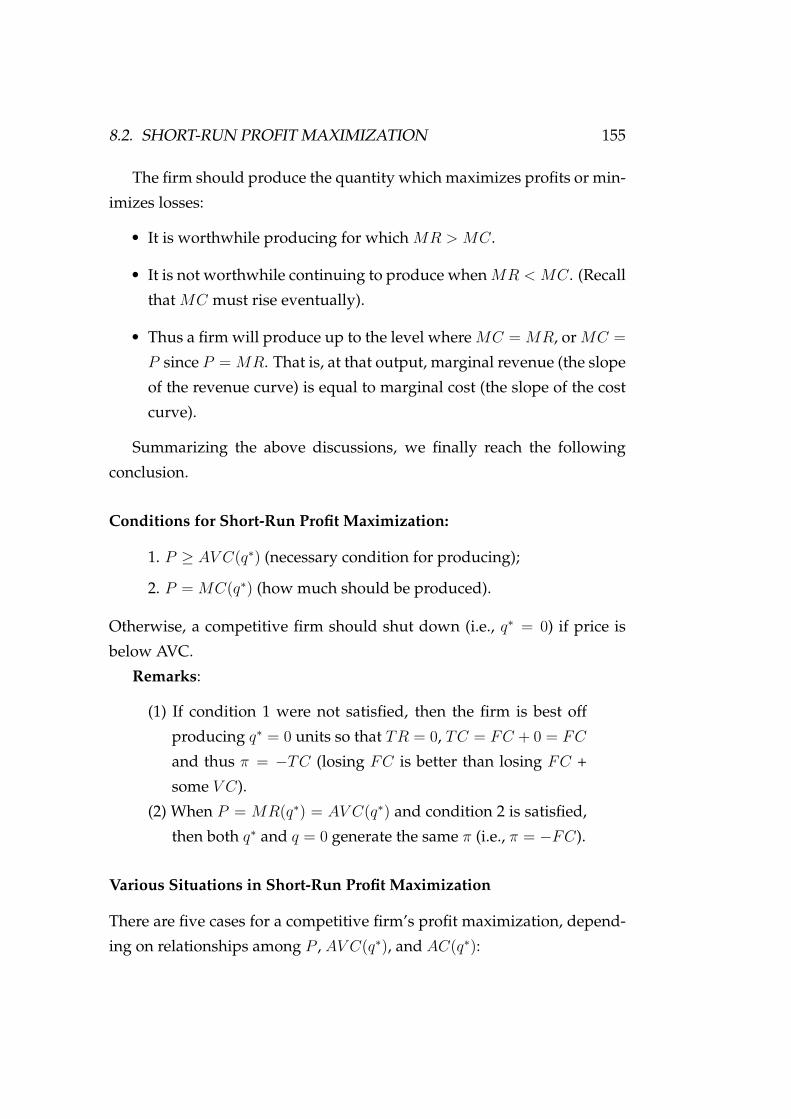
8.2. SHORT-RUN PROFIT MAXIMIZATION 155
The firm should produce the quantity which maximizes profits or min-
imizes losses:
• It is worthwhile producing for which MR > MC.
• It is not worthwhile continuing to produce when MR < MC. (Recall
that MC must rise eventually).
• Thus a firm will produce up to the level where MC = MR, or MC =P since P = MR. That is, at that output, marginal revenue (the slope
of the revenue curve) is equal to marginal cost (the slope of the cost
curve).
Summarizing the above discussions, we finally reach the following
conclusion.
Conditions for Short-Run Profit Maximization:
1. P ≥ AV C(q∗) (necessary condition for producing);
2. P = MC(q∗) (how much should be produced).
Otherwise, a competitive firm should shut down (i.e., q∗ = 0) if price is
below AVC.
Remarks:
(1) If condition 1 were not satisfied, then the firm is best off
producing q∗ = 0 units so that TR = 0, TC = FC + 0 = FC
and thus π = −TC (losing FC is better than losing FC +
some V C).
(2) When P = MR(q∗) = AV C(q∗) and condition 2 is satisfied,
then both q∗ and q = 0 generate the same π (i.e., π = −FC).
Various Situations in Short-Run Profit Maximization
There are five cases for a competitive firm’s profit maximization, depend-
ing on relationships among P , AV C(q∗), and AC(q∗):

156 CHAPTER 8. PROFIT MAXIMIZATION AND COMPETITIVE FIRM
Case 1: P > AC(q∗), resulting in positive profit;
Case 2: P = AC(q∗), zero profit;
Case 3: AC(q∗) > P > AV C(q∗), loss minimization;
Case 4: AC(q∗) > P = AV C(q∗), no difference between producing q∗ and
shutdown (q = 0) since Loss = TFC in either case;
Case 5: P < AC(q∗), shutdown.
As shown in Figure 8.3, when the price is P1, the profit-maximizing
output is q1. The total profits are the rectangle ABCD. When the price is
P2, the most profitable output is q2. The profits, however, are zero since
the price just equals average cost of production. When the price is P3, the
firm can just cover its variable cost by producing q3, where AV C equals
the price. At this point the firm would be operating at a short-run loss; the
loss is exactly equal to its total fixed cost. At a price below P3 the firm is
unable to cover its variable cost and hence must shut down.
$
Q
MC
P�=MR
AC
AVCP =MR
P!=MR
q�q q!
AD
BC
Figure 8.3 Profit maximization in the short run
Let us consider some numerical examples.

8.2. SHORT-RUN PROFIT MAXIMIZATION 157
q AFC AV C ATC MC TC P = AR = MR TR π
0 − − − − − − − − − − − − 100 131 0 100
1 100 90 190 90 190 131 131 -59
2 50 85 135 80 270 131 262 -8
3 3313 80 1131
3 70 340 131 393 53
4 25 75 100 60 400 131 524 124
5 20 74 94 70 470 131 655 185
6 1623 75 912
3 80 550 131 786 236
7 1427 771
7 9137 90 640 131 917 277
8 1212 811
4 9334 110 750 131 1048 298
9 1119 862
3 9779 130 880 131 1179 299
10 10 93 103 150 1030 131 1310 280
Table 8.1
Example 8.1 (Perfect Competition: Profit Maximization) Note that TC =ATC × q, and TR = p × q. From Table 8.1, we know MR > MC for
q = 1, 2, ..., 9. MR < MC for q = 10. q = 9 for profit maximization. Since
AR > ATC at q = 9, a positive profit is made.
$
Q
MC
P=AR=MR
AVC
ATC
O
ab
cd
q*
Figure 8.4 Identifying profit-maximizing output and short-run profit
From Figure 8.4, we know TR = AR × q∗ = Oabq∗, TC = ATC × q∗ =Odcq∗, Profit = TR − TC = abcd. At point b in Figure 8.4, MR = MC ⇒q∗ = 9.
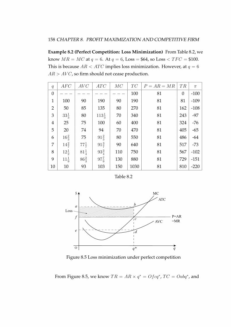
158 CHAPTER 8. PROFIT MAXIMIZATION AND COMPETITIVE FIRM
Example 8.2 (Perfect Competition: Loss Minimization) From Table 8.2, we
know MR = MC at q = 6. At q = 6, Loss = $64, so Loss < TFC = $100.
This is because AR < ATC implies loss minimization. However, at q = 6AR > AV C, so firm should not cease production.
q AFC AV C ATC MC TC P = AR = MR TR π
0 − − − − − − − − − − − − 100 81 0 -100
1 100 90 190 90 190 81 81 -109
2 50 85 135 80 270 81 162 -108
3 3313 80 1131
3 70 340 81 243 -97
4 25 75 100 60 400 81 324 -76
5 20 74 94 70 470 81 405 -65
6 1623 75 912
3 80 550 81 486 -64
7 1427 771
7 9137 90 640 81 517 -73
8 1212 811
4 9334 110 750 81 567 -102
9 1119 862
3 9779 130 880 81 729 -151
10 10 93 103 150 1030 81 810 -220
Table 8.2
MC
P=AR
=MRAVC
ATC
O
a b
c
de
f
q* q
Loss
$
Figure 8.5 Loss minimization under perfect competition
From Figure 8.5, we know TR = AR × q∗ = Ofcq∗, TC = Oabq∗, and

8.2. SHORT-RUN PROFIT MAXIMIZATION 159
Loss = TC − TR = abcf . At point c in Figure 8.5, MR = MC ⇒ q∗ = 6.
Example 8.3 (Perfect Competition: Production Shutdown) From Table 8.3,
we know MR = MC at q = 5 which looks optimal. However, AR < AV C
at q = 5, which implies Loss > TFC (115 > 100). Thus loss is minimized
only when q = 0, i.e., shutting down production is optimal.
From Figure 8.6, we know at point d in Figure 8.6, MR = MC ⇒ q∗ =5.
At q∗ = 5, TR = Oedq∗, TC = Oabq∗, ⇒ Loss = eabd.
At q = 0, TR = 0, TC = TFC = AFC × q = abcf , which is
small than eabd.
Thus shutdown is optimal.
q AFC AV C ATC MC TC P = AR = MR TR π
0 − − − − − − − − − − − − 100 − − − − − − -100
1 100 90 190 90 190 71 71 -119
2 50 85 135 80 270 71 142 -128
3 3313 80 1131
3 70 340 71 213 -127
4 25 75 100 60 400 71 284 -116
5 20 74 94 70 470 71 355 -115
6 1623 75 912
3 80 550 71 426 -124
7 1427 771
7 9137 90 640 71 497 -143
8 1212 811
4 9334 110 750 71 568 -182
9 1119 862
3 9779 130 880 71 639 -241
10 10 93 103 150 1030 71 710 -320
Table 8.3

160 CHAPTER 8. PROFIT MAXIMIZATION AND COMPETITIVE FIRM
MC
P=AR=MR
AVC
ATC
O
a b
c
de
f
q* q
Loss if
shutdown
$
Figure 8.6 Production shutdown under perfect competition
Example 8.4 Suppose TC(q) = 200 + 9q + 5q2, MC(q) = 9 + 10q, and
P = 16.
(a) Find the AV C. AV C = V Cq
where V C is the portion of TC
which involves terms with “q”:
V C(q) = 9q + 5q2.
Thus AV C = 9q+5q2
q= 9 + 5q.
(b) Find the profit-maximizing level of output.
• P = MC(q∗) ⇒ 16 = 9 + 10q ⇒ q∗ = 710 .
• P ≥ AV C(q∗)?
AV C(q∗) = 9 + 5q∗ = 9 + 5 × 710 = 9 + 7
2 = 12.5 < 16.
Thus P ≥ AV C(q∗), and hence q∗ = 710 is indeed profit-
maximizing level of output.
Note: If we change P , we find a new q∗. Repeating this we can draw a
supply curve.

8.3. COMPETITIVE FIRM’S SHORT-RUN SUPPLY CURVE 161
8.3 Competitive Firm’s Short-run Supply Curve
From the conditions for short-run profit maximization, we know that the
firm chooses its output so that marginal cost MC is equal to price as long
as the firm covers its average variable cost, and also MC = P shows that
a competitive firm will produce more at higher price levels because in-
creased production becomes profitable at higher prices.
Thus, the firm’s supply curve is the portion of the marginal cost curve
that lies above the minimum average variable cost.
The short-run supply curve is given by the crosshatched portion of the
marginal cost curve as in Figure 8.7.
Price
(dollars per
unit)
P=AVC
Outputq1q
2
P!
P"
AVC
AC
MC
Figure 8.7 Output response to an input price reduction
8.4 Output Response to a Change in Input Prices
A change in the price of an input, combined with an unchanged output
price, will change the profit-maximizing level of output. If the price of an
input falls, MC shifts to MC ′, and output increases, where MC ′ equals the
unchanged output price.
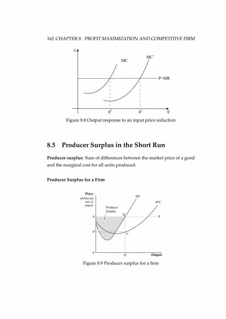
162 CHAPTER 8. PROFIT MAXIMIZATION AND COMPETITIVE FIRM
MC
P=MR
q q
$
MC
q!
Figure 8.8 Output response to an input price reduction
8.5 Producer Surplus in the Short Run
Producer surplus: Sum of differences between the market price of a good
and the marginal cost for all units produced.
Producer Surplus for a Firm
Price
Output
(dollars per
unit of
output)
0
AB
CD
MC
AVC
P
q*
Producer
Surplus
Figure 8.9 Producer surplus for a firm

8.5. PRODUCER SURPLUS IN THE SHORT RUN 163
The producer surplus (PS) for a firm is measured by the shaded area be-
low the market price and above the marginal cost curve, between outputs
0 and q*, the profit-maximizing output in Figure 8.9
Alternatively, it is equal to rectangle ABCD because the sum of al-
l marginal costs up to q∗ is equal to the variable costs of producing q∗.
That is,
PS = TR − TV C.
The difference between producer surplus and profit of a firm is then
the total fixed cost since
π = TR − TV C − TFC = PS − TFC.
Producer Surplus for a Market
The producer surplus for a market is the area below the market price and
above the market supply curve, between 0 and output Q* as depicted in
Figure 8.10.
Price
Output
(dollars per
unit of
output)
0
D
P*
q*
Producer
Surplus
S
Figure 8.10 Producer surplus for a market

164 CHAPTER 8. PROFIT MAXIMIZATION AND COMPETITIVE FIRM
8.6 Long-Run Profit Maximization
The same principle used for the short-run setting can apply to the discus-
sion of long-run profit maximization, but now we employ long-run cost
curves. The firm maximizes profits in the long run by producing up to
where P = MC. That is, the long-run output of a profit-maximizing com-
petitive firm is the point at which long-run marginal cost equals the price.
MC
P*=MR
LAC
O q� q
$
A
B
D
C
SMC SAC
E
FC
q
Figure 8.11 The long-run output of a profit-maximizing competitive firm
With a price P ∗, the most profitable output will be q1 in the long run,
and the profit is rectangle ABCD. In the short run the most profitable
output will be q2, and rectangle CEFC1 is the profit which is less than the
long-run profit.
Conditions for Long-Run Profit Maximization:
(1): P ≥ AC (necessary condition for producing);
(2): P = MC (how much should be produced).
Note that producer surplus coincides with profit of a firm since the
total fixed cost equals zero in the long-run.
Chapter 9
Competitive Markets
In this chapter the emphasis shifts from the individual firm to the compet-
itive industry/markets.
Assumptions on Perfect Competitive Markets:
• A large number of buyers and sellers, which will normally guaran-
tee that the firms and consumers behave as price takers.
• Unrestricted mobility of resources: no barrier to entry into, or exit
from the market.
• Homogeneous products: the products of all of the firms in an indus-
try are identical to consumers.
• Possession of all relevant information to make economic decisions.
Unrestricted mobility implies that there are no special costs that make
it difficult for a firm to enter (or exit) an industry. With free entry and exit,
buyers can easily switch from one supplier to another, and suppliers can
easily enter or exit a market.
The presence of many firms is not sufficient for an industry to approx-
imate perfect competition since firms can implicitly or explicitly collude
in setting prices. Conversely, the presence of only a few firms in a market
does not rule out competitive behavior.
165

166 CHAPTER 9. COMPETITIVE MARKETS
When Is a Market Highly Competitive? Many markets are highly
competitive in the sense that firms face highly elastic demand curves and
relatively easy entry and exit, but there is no simple rule of thumb to de-
scribe whether a market is close to being perfectly competitive.
9.1 The Short-Run Industry Supply Curve
In the short run a competitive firm will produce at a point where the
marginal cost equals the price, as long as the price is above the minimum
point of its average variable cost curve.
How is the short-run industry supply curve determined?
The horizontal sum of MC curves for each firm (above AV C) gives the
industry supply curve. That is, the short run industry supply curve is de-
rived by simply adding the quantities produced by all individual firms.
q q!q" Q=q +q"+q! Q
P
P
P
P
P!
P"
MC! MC" MC# SS
D
D’
Q’
Figure 9.1 The short-run industry supply curve
Note that the short-run supply curve, SS, slopes upward. Recall that
each firm’s marginal cost curve slopes upward because it reflects the law
of diminishing marginal returns to variable inputs. Thus, the law of di-
minishing marginal returns is the underlying determinant of the shape of
a competitive industry’s short-run supply curve.

9.2. LONG-RUN COMPETITIVE EQUILIBRIUM 167
Price and Output Determination in the Short Run
The interaction of supply and demand in a market determines market
price and output. In Figure 9.1 the intersection of the demand curve D
with the supply curve SS pins down the price where total quantity de-
manded equals total quantity supplied. Thus P is the equilibrium price
and equilibrium industry output is Q, where Q = q1 + q2 + q3.
In the short run an increase in market demand leads to a higher price
and higher output. When demand increases to D′, the equilibrium price
becomes P ′ and industry output is now Q′.
9.2 Long-Run Competitive Equilibrium
Firm Market
S
D
P=MR
LMCP
Figure 9.2 The emergence of long-run competitive equilibrium
In the long-run competitive equilibrium, the independent plans of firms
and consumers mesh perfectly. Each firm has adjusted its scale of opera-
tion in light of the prevailing price and is able to sell as mush as it chooses
to sell. Consumers are able to purchase as much as they wish to consume
at the prevailing price. There are no incentives for any firm to alter its scale
of operation or to exit from the industry and no incentive for outsiders to
enter the market. Unless the underlying market conditions change, the
price and rate of output will remain stable.

168 CHAPTER 9. COMPETITIVE MARKETS
Long-Run Competitive Equilibrium:
(a) Profit maximization: Each firm must be producing the out-
put level such that its profit is maximized at the prevailing
market price, that is, P = LMC.
(b) Zero economic profit made by each firm. There are no in-
centives for firms to either enter or exit from the industry.
(c) Market quantity supplied equals market quantity demand-
ed: The combined quantity of outputs of all firms at the pre-
vailing price must equal the total quantity consumers wish
to purchase at that price level.
Zero economic profit: A firm is earning a normal return on its invest-
ment in a perfectly competitive market — i.e., it is doing as well as it could
by investing its money elsewhere.
Remarks: There are instances in which firms earning positive account-
ing profit may be earning zero economic profit. If a clothing store is be
located near a large shopping center, the additional flow of customers can
increase the store’s accounting profit. When the opportunity cost of the
land is included, the profitability of the clothing store is no higher than
that of its competitors.
Entry and exit
In a market with entry and exit, a firm enters when it can earn a positive
long-run profit and exits when it faces the prospect of a long-run loss.
Entry of Firms Eliminates Profits:
(i) In Figure 9.3, the representative firm is in a long-run equi-
librium. P e = minimum point of ATC. Normal profits are
earned, and hence economic profit = 0.
(ii) Suppose demand increases from D1 to D2. Price rises to
p1 and exceeds the minimum point of ATC. Thus, positive
economic profits are earned.

9.2. LONG-RUN COMPETITIVE EQUILIBRIUM 169
(iii) New firms enter the industry. Supply starts to increase
from S1, and then price starts to fall.
(iv) Supply continues to increase while economic profits are be-
ing made. The increase of supply will not stop until it reach-
es the new supply curve S2, where P e = minimum point of
ATC again.
(v) In the long run, a larger quantity is supplied at the same
initial price level.
Firm Industry
S
D!
MC
Pe
q
ATC
S"
D#
qqe2
qe1
P
Figure 9.3 Entry of firms eliminates economic profits
Exit of Firms Eliminates Losses:
(i) In Figure 9.4, the representative firm is in a long-run equi-
librium. P e = minimum point of ATC. Normal profits are
earned, and hence no economic profits could be generated.
(ii) Suppose demand decreases from D1 to D3. Price falls below
the minimum point of ATC to p2 . Economic profits are
negative, i.e., firms suffer from economic losses.
(iii) Firms leave the industry and supply falls from S1, causing
price to rise.
(iv) Supply continues to fall while economic loss is being ex-
perienced. The reduction of supply will not stop until it

170 CHAPTER 9. COMPETITIVE MARKETS
reaches the new one S3 where pe = the minimum point of
ATC again.
(v) In the long run, a smaller quantity is produced and supplied
at the same initial price.
Firm Industry
S
D!
MC
Pe
q
ATC
S"
D#
qqe1
qe3
P$
Figure 9.4 Exit of firms eliminates losses
9.3 The Long-Run (LR) Supply Curve
Economists distinguish among three different types of competitive indus-
tries, constant-cost, increasing-cost, and decreasing-cost. The distinction
depends on how a change in industry output affects the prices of inputs.
Constant-Cost Industry: Horizontal LR Supply Curve
Constant-Cost Industry: Expansion of output does not affect input prices,
and consequently the entry and exit of firm do not cause cost curves to
shift. The price of output remains constant for all levels of quantity, and
hence LR supply is perfectly elastic. The long-run supply curve for a
constant-cost industry is, therefore, a horizontal line at a price that is e-
qual to the long-run minimum average cost of production.

9.3. THE LONG-RUN (LR) SUPPLY CURVE 171
Firm Industry
SS
D!
SMC
P
LAC
SS"
D#
LMC
MR
P’
q1
P’
P
D$
LS
q2 Q Q" Q%
Figure 9.5 The long-run supply curve for a constant-cost industry
Increasing-Cost Industry: Upward-Sloping LR Supply Curve
Firm Industry
SS
D
SMC
P
LAC
SS
D!
MR
P’
q1
P’
P
q2 Q" Q# Q$
SMC LAC
MR
q3
P’’ P’’
LS
A
B
C
Figure 9.6 The long-run supply curve for an increasing-cost industry
Increasing-Cost Industry: Expansion of output causes input prices to rise
as demand for them grow, and consequently the entry/exit of firm makes
cost curves shift upward/downward. As firms enter the industry, they
compete for scarce resources. Therefore, prices of input resources rise as
do production costs of firms. So cost curves shift upward (ATC and MC).
Hence industry supply curve is upward-sloping.
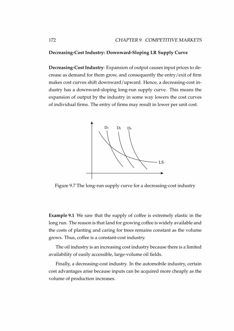
172 CHAPTER 9. COMPETITIVE MARKETS
Decreasing-Cost Industry: Downward-Sloping LR Supply Curve
Decreasing-Cost Industry: Expansion of output causes input prices to de-
crease as demand for them grow, and consequently the entry/exit of firm
makes cost curves shift downward/upward. Hence, a decreasing-cost in-
dustry has a downward-sloping long-run supply curve. This means the
expansion of output by the industry in some way lowers the cost curves
of individual firms. The entry of firms may result in lower per unit cost.
LS
D� D� D�
Figure 9.7 The long-run supply curve for a decreasing-cost industry
Example 9.1 We saw that the supply of coffee is extremely elastic in the
long run. The reason is that land for growing coffee is widely available and
the costs of planting and caring for trees remains constant as the volume
grows. Thus, coffee is a constant-cost industry.
The oil industry is an increasing cost industry because there is a limited
availability of easily accessible, large-volume oil fields.
Finally, a decreasing-cost industry. In the automobile industry, certain
cost advantages arise because inputs can be acquired more cheaply as the
volume of production increases.
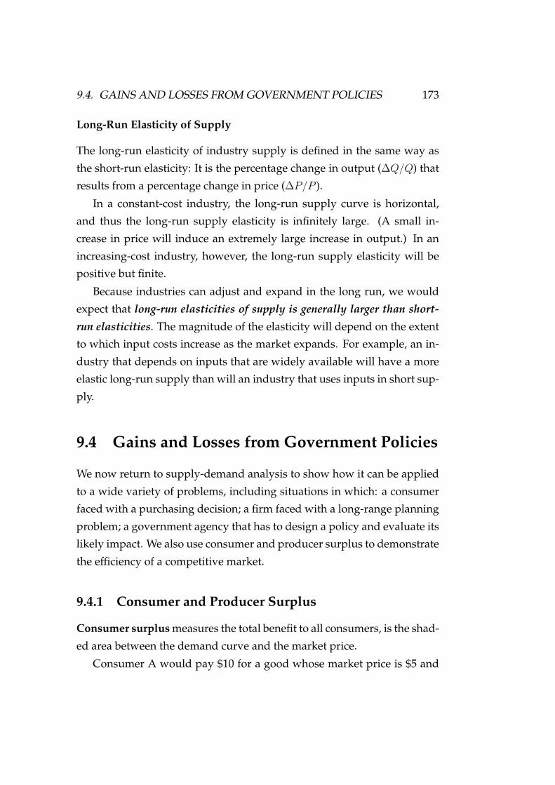
9.4. GAINS AND LOSSES FROM GOVERNMENT POLICIES 173
Long-Run Elasticity of Supply
The long-run elasticity of industry supply is defined in the same way as
the short-run elasticity: It is the percentage change in output (∆Q/Q) that
results from a percentage change in price (∆P/P ).
In a constant-cost industry, the long-run supply curve is horizontal,
and thus the long-run supply elasticity is infinitely large. (A small in-
crease in price will induce an extremely large increase in output.) In an
increasing-cost industry, however, the long-run supply elasticity will be
positive but finite.
Because industries can adjust and expand in the long run, we would
expect that long-run elasticities of supply is generally larger than short-
run elasticities. The magnitude of the elasticity will depend on the extent
to which input costs increase as the market expands. For example, an in-
dustry that depends on inputs that are widely available will have a more
elastic long-run supply than will an industry that uses inputs in short sup-
ply.
9.4 Gains and Losses from Government Policies
We now return to supply-demand analysis to show how it can be applied
to a wide variety of problems, including situations in which: a consumer
faced with a purchasing decision; a firm faced with a long-range planning
problem; a government agency that has to design a policy and evaluate its
likely impact. We also use consumer and producer surplus to demonstrate
the efficiency of a competitive market.
9.4.1 Consumer and Producer Surplus
Consumer surplus measures the total benefit to all consumers, is the shad-
ed area between the demand curve and the market price.
Consumer A would pay $10 for a good whose market price is $5 and

174 CHAPTER 9. COMPETITIVE MARKETS
therefore enjoys a benefit of $5. Consumer B enjoys a benefit of $2, and
Consumer C, who values the good at exactly the market price, enjoys no
benefit.
Price
Quantity
5
7
$10
D
Q0
Consumer Surplus
S
Consumer A Consumer B Consumer C
Figure 9.8 Consumer surplus
Price
Quantity
5
7
$10
D
Q0
Consumer Surplus
S
Consumer A Consumer B Consumer C
Producer
Surplus
Figure 9.9 Consumer and producer surplus

9.4. GAINS AND LOSSES FROM GOVERNMENT POLICIES 175
Producer surplus measures the total profits of producers, plus rents to
factor inputs. It is the benefit that lower-cost producers enjoy by selling
at the market price, shown by the shaded area between the supply curve
and the market price.
Together, consumer and producer surplus measure the welfare benefit
of a competitive market as shown in Figure 9.9.
Deadweight loss: Net loss of total (consumer plus producer) surplus.
Welfare Effects Gains and Losses to Consumers and Producers
The price of a good has been regulated to be no higher than ceiling price
Pmax, which is below the market-clearing price P0. The gain to consumers
is the difference between rectangle A and triangle B. The loss to produc-
ers is the sum of rectangle A and triangle C. Triangles B and C together
measure the deadweight loss from price controls.
Price
Quantity
S
D
{
Shortage
P0
Pmax
Q0 Q2Q1
Deadweight Loss
A C
B
A
B
CC
Figure 9.10 Change in consumer and producer surplus from price control
If demand is sufficiently inelastic, triangle B can be larger than rect-
angle A. In this case, consumers suffer a net loss from price controls as
shown in Figure 9.11.
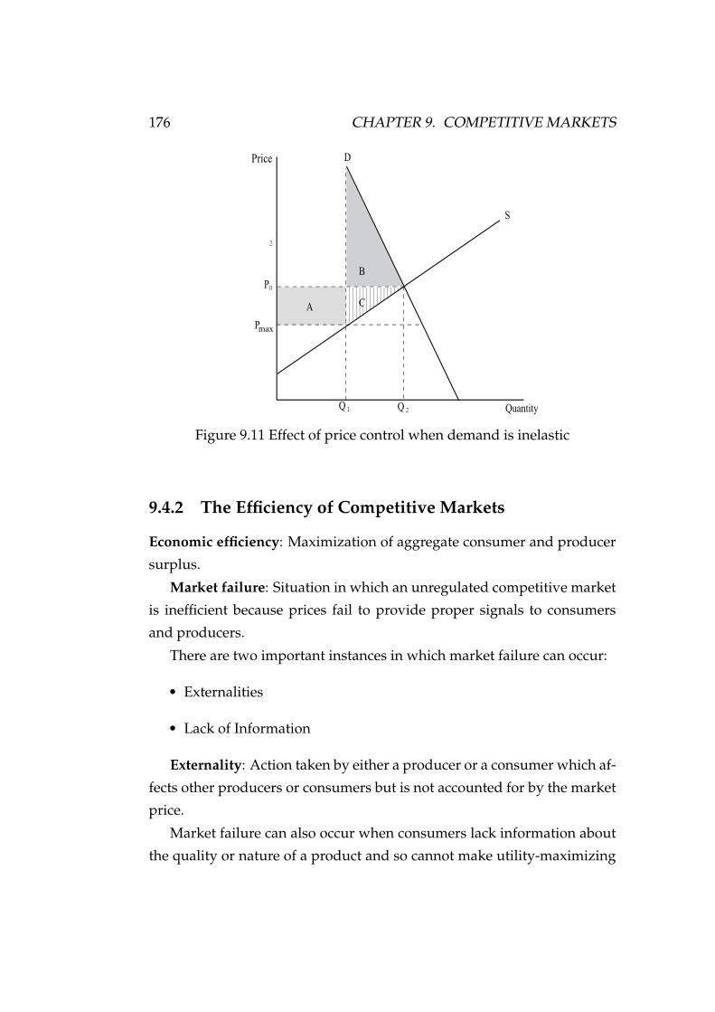
176 CHAPTER 9. COMPETITIVE MARKETS
Price
Quantity
S
D
P
2
Q2Q1
A C
B
CC
P0
max
Figure 9.11 Effect of price control when demand is inelastic
9.4.2 The Efficiency of Competitive Markets
Economic efficiency: Maximization of aggregate consumer and producer
surplus.
Market failure: Situation in which an unregulated competitive market
is inefficient because prices fail to provide proper signals to consumers
and producers.
There are two important instances in which market failure can occur:
• Externalities
• Lack of Information
Externality: Action taken by either a producer or a consumer which af-
fects other producers or consumers but is not accounted for by the market
price.
Market failure can also occur when consumers lack information about
the quality or nature of a product and so cannot make utility-maximizing

9.5. MINIMUM PRICES (PRICE FLOOR) 177
purchasing decisions. Government intervention (e.g., requiring “truth in
labeling”) may then be desirable.
In the absence of externalities or a lack of information, an unregulated
competitive market does lead to the economically efficient output level.
To see this, suppose that price is regulated to be no lower than P2, and
then only Q3 will be demanded. If Q3 is produced, the deadweight loss is
given by triangles B and C. At price P2, producers would like to produce
more than Q3. If they do, the deadweight loss will be even larger, as shown
in Figure 9.12.
Price
Quantity
S
D
P2
Q0Q3
A
C
BP0
Q2
Figure 9.12 Welfare loss when price is held above market-clearing level
9.5 Minimum Prices (Price Floor)
Minimum price is also known the price floor or price support, which is
the price higher than the market price. Suppose that price is regulated to
be no lower than Pmin as in Figure 9.13. Producers would like to supply
Q2, but consumers will buy only Q3. Then the amount Q2 − Q3 will go
unsold and the change in producer surplus will be A − C − D. In this case,

178 CHAPTER 9. COMPETITIVE MARKETS
producers as a group may be worse off.
The total change in consumer surplus is:
∆CS = −A − B.
Price
Quantity
S
D
Pmin
Q0Q3
A
C
BP0
Q2
D
Figure 9.13 Price minimum
The total change in producer surplus is
∆PS = A − C − D.
Minimum Wage
Although the market-clearing wage is w0, firms are not allowed to pay less
than wmin.
This results in unemployment of an amount L2 − L1 and a deadweight
loss given by triangles B and C in Figure 9.14.
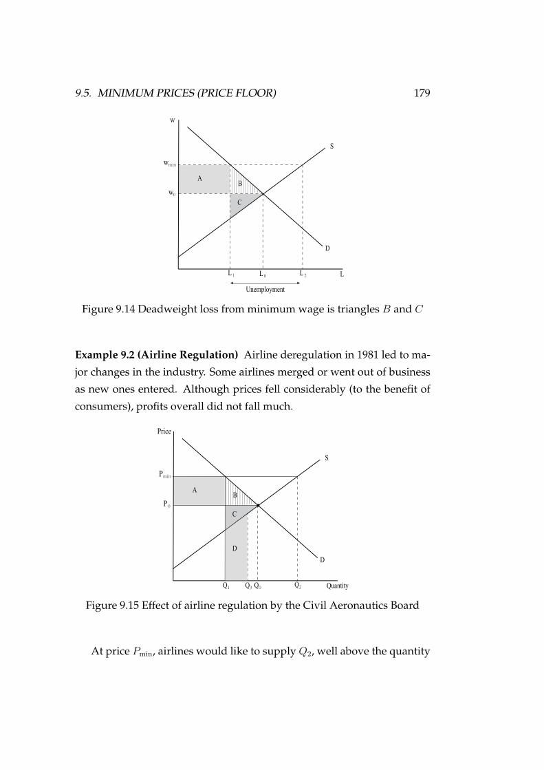
9.5. MINIMUM PRICES (PRICE FLOOR) 179
L
S
D
wmin
L 0L 1
A
C
Bw0
L 2
w
Unemployment
Figure 9.14 Deadweight loss from minimum wage is triangles B and C
Example 9.2 (Airline Regulation) Airline deregulation in 1981 led to ma-
jor changes in the industry. Some airlines merged or went out of business
as new ones entered. Although prices fell considerably (to the benefit of
consumers), profits overall did not fall much.
Quantity
S
D
Pmin
Q0Q1
A
C
BP 0
Q2
Price
D
Q3
Figure 9.15 Effect of airline regulation by the Civil Aeronautics Board
At price Pmin, airlines would like to supply Q2, well above the quantity
180 CHAPTER 9. COMPETITIVE MARKETS
Q1 that consumers will buy.
When they supply Q3, trapezoid D is the cost of unsold output. Airline
profits may have been lower as a result of regulation because triangle C
and trapezoid D can together exceed rectangle A. In addition, consumers
lose A + B.

Part IV
Market Structure and Competitive
Strategy
181


183
Part 3 examines a broad range of markets and explains how the pricing,
investment, and output decisions of firms depend on market structure and
the behavior of competitors.

184

Chapter 10
Monopoly and Monopsony
While perfect competition is characterized by many firms selling in the
same market, monopoly is characterized by only one firm selling in a giv-
en market. In this chapter, we explain how a monopoly determines price
and output, and compare the results with those of the competitive indus-
try. We will then discuss monopsony which is characterized by only one
buyer of a good.
10.1 The Nature of Monopoly
Monopoly: A form of market structure in which there is only one seller of
some product that has no close substitutes. As a result, the monopoly is
the industry because it is the only producer in the market.
Monopoly is the opposite of perfect competition since there is no com-
petition. The monopoly need not be concerned with the possibility that
other firms may undercut its price.
Monopsony: Market with only one buyer.
Market power (also known the monopoly power for a seller or monop-
sony power for a buyer): Ability of a seller or buyer to affect the price of a
good.
185
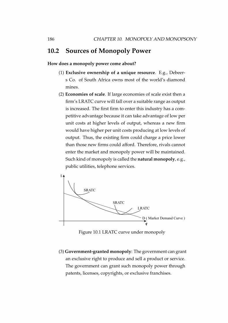
186 CHAPTER 10. MONOPOLY AND MONOPSONY
10.2 Sources of Monopoly Power
How does a monopoly power come about?
(1) Exclusive ownership of a unique resource. E.g., Debeer-
s Co. of South Africa owns most of the world’s diamond
mines.
(2) Economies of scale. If large economies of scale exist then a
firm’s LRATC curve will fall over a suitable range as output
is increased. The first firm to enter this industry has a com-
petitive advantage because it can take advantage of low per
unit costs at higher levels of output, whereas a new firm
would have higher per unit costs producing at low levels of
output. Thus, the existing firm could charge a price lower
than those new firms could afford. Therefore, rivals cannot
enter the market and monopoly power will be maintained.
Such kind of monopoly is called the natural monopoly, e.g.,
public utilities, telephone services.
$
SRATC
SRATC
LRATC
D ( Market Demand Curve )
q
Figure 10.1 LRATC curve under monopoly
(3) Government-granted monopoly: The government can grant
an exclusive right to produce and sell a product or service.
The government can grant such monopoly power through
patents, licenses, copyrights, or exclusive franchises.
10.2. SOURCES OF MONOPOLY POWER 187
• patents: give inventor a monopoly position for life-
time of patent–17 years after the patent was granted
in the U.S.A. E.g., IBM, Xerox.
• copyrights: give writers and composers exclusive le-
gal controls over production and reproduction of their
work for 70 years after the death of the author.
• licenses: limit the number of producers but rarely give
monopoly power. E.g., licenses are needed to practice
medicine, law, cut hair, or sell liquor.
• public utilities: competition is impractical so indus-
tries are given exclusive franchise by the government.
If firms share the market none would be able to take
advantage of the large economies of scale. If only one
firm supplied in the market it could take advantage
of the lower per unit costs. In return for the granted
monopoly position, the government is allowed to reg-
ulate the price of the product.
(4) The interaction among firms:
• Even if only two or three firms are in the market, firms
might compete aggressively, undercutting one anoth-
er’s prices to capture more market share, or they might
not compete much. They might even collude (in vio-
lation of the antitrust laws), agreeing to limit output
and raise prices. Other things being equal, monopoly
power is smaller when firms compete aggressively and
is larger when they cooperate. Because raising prices
in concert rather than individually is more likely to be
profitable, collusion can generate substantial monopoly
power.

188 CHAPTER 10. MONOPOLY AND MONOPSONY
• Remember that a firm’s monopoly power often changes
over time, as its operating conditions (market demand
and cost), its behavior, and the behavior of its com-
petitors change. Monopoly power must therefore be
thought of in a dynamic context.
• Furthermore, real or potential monopoly power in the
short run can make an industry more competitive in
the long run: Large short-run profits can induce new
firms to enter an industry, thereby reducing monopoly
power over the longer term.
10.3 The Monopoly’s Demand and Marginal Rev-
enue Curves
D
P
q
P
P!
q1q2
Figure 10.2 Downward-sloping demand curve under monopoly
Under perfect competition each firm is a price taker and thus faces a hori-
zontal demand curve. By contract, the monopolist comprises the entire in-
dustry. Thus, the firm’s (monopolist’s) demand curve is industry demand
curve. Then a monopolist’s demand curve is downward sloping—i.e., the
firm is a price “maker”. Recall that
• TR: Total Revenue = P × Q;

10.3. THE MONOPOLY’S DEMAND AND MARGINAL REVENUE CURVES189
• MR: Marginal Revenue = ∆T R∆Q
;
• AR: Average Revenue = P ×QQ
= P .
Since the demand curve is always the AR curve, which is downward
sloping for a monopolist, marginal revenue must be less than average rev-
enue. Since AR = P , we generally have MR < P .
Consider a firm facing the following demand curve: P = 11 − Q.
Q P =AR TR MR0 $11 0 −1 10 10 102 9 18 83 8 24 64 7 28 45 6 30 26 5 30 07 4 28 -28 3 24 -49 2 18 -610 1 10 -8
Note that
MR = ∆TR
∆Q= P∆Q + Q∆P
∆Q= P + Q
∆P
∆Q. (10.1)
Since Q > 0 and ∆P∆Q
< 0, again we have MR < P.
Intuitively, the extra revenue from an incremental unit of quantity has
two components:
• Producing one extra unit and selling it at P brings in revenue P .
• But because the firm faces a downward-sloping demand curve, pro-
ducing and selling this extra unit also results in a small drop in price
∆P/∆Q, which reduces the revenue from all units sold (i.e., a change
in revenue q × ∆P/∆Q).
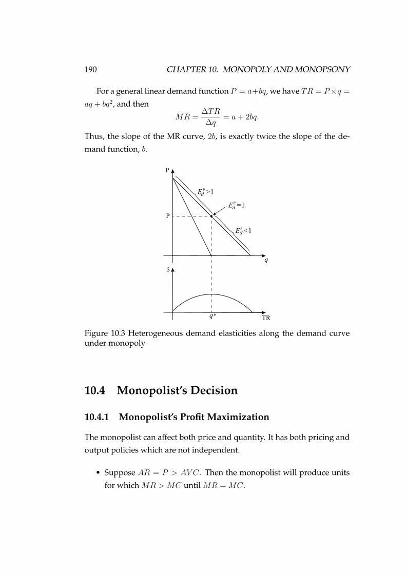
190 CHAPTER 10. MONOPOLY AND MONOPSONY
For a general linear demand function P = a+bq, we have TR = P ×q =aq + bq2, and then
MR = ∆TR
∆q= a + 2bq.
Thus, the slope of the MR curve, 2b, is exactly twice the slope of the de-
mand function, b.
TR
P
q
P
$
q*
}}E >1
P
d
E <1dP
E =1dP
Figure 10.3 Heterogeneous demand elasticities along the demand curveunder monopoly
10.4 Monopolist’s Decision
10.4.1 Monopolist’s Profit Maximization
The monopolist can affect both price and quantity. It has both pricing and
output policies which are not independent.
• Suppose AR = P > AV C. Then the monopolist will produce units
for which MR > MC until MR = MC.

10.4. MONOPOLIST’S DECISION 191
• Suppose AR = P < AV C for all levels of output (the market demand
is below AV C). Then the profit-maximizing output is Q = 0.
Conditions for monopolist’s profit maximization:
1) P ≥ AV C (necessary condition for producing);
2) MR = MC (how much will it be produced).
P
q
P*
P=AR
≡demand
MR
q*
MC
Figure 10.4 Monopolist’s profit-maximizing output
We can express profit maximization, loss minimization, shutdown, and
normal profit graphically, which depend on relationships among price P ,
average total cost ATC, and average variable cost AV C.
Profit Maximization: P > ATC > AV C
MC
P*=AR*
ATC
O q
P
q*
P=AR
AVC
MR
Figure 10.5 Profit maximization for a monopolist

192 CHAPTER 10. MONOPOLY AND MONOPSONY
1. Use MR = MC to determine q∗.
2. Use q∗ and P = AR (= demand) to decide P ∗.
3. TR = AR × q∗ = P ∗ × q∗.
4. Use q∗ and ATC to get TC. TC = ATC × q∗.
5. Profit = TR − TC.
Loss Minimization: ATC > P > AV C
MC
P*=AR*
ATC
O
P
q*
P=AR
AVC
MR
ATC*
minimum
loss
q
Figure 10.6 Loss minimization for a monopolist
Production Shutdown: ATC > AV C > P
MC
P*=AR*
ATC
O Q
P
q*
P=AR
AVC
MR
ATC* }AFC
Figure 10.7 Production shutdown for a monopolist
q∗ = 0 is the loss-minimizing level of output.
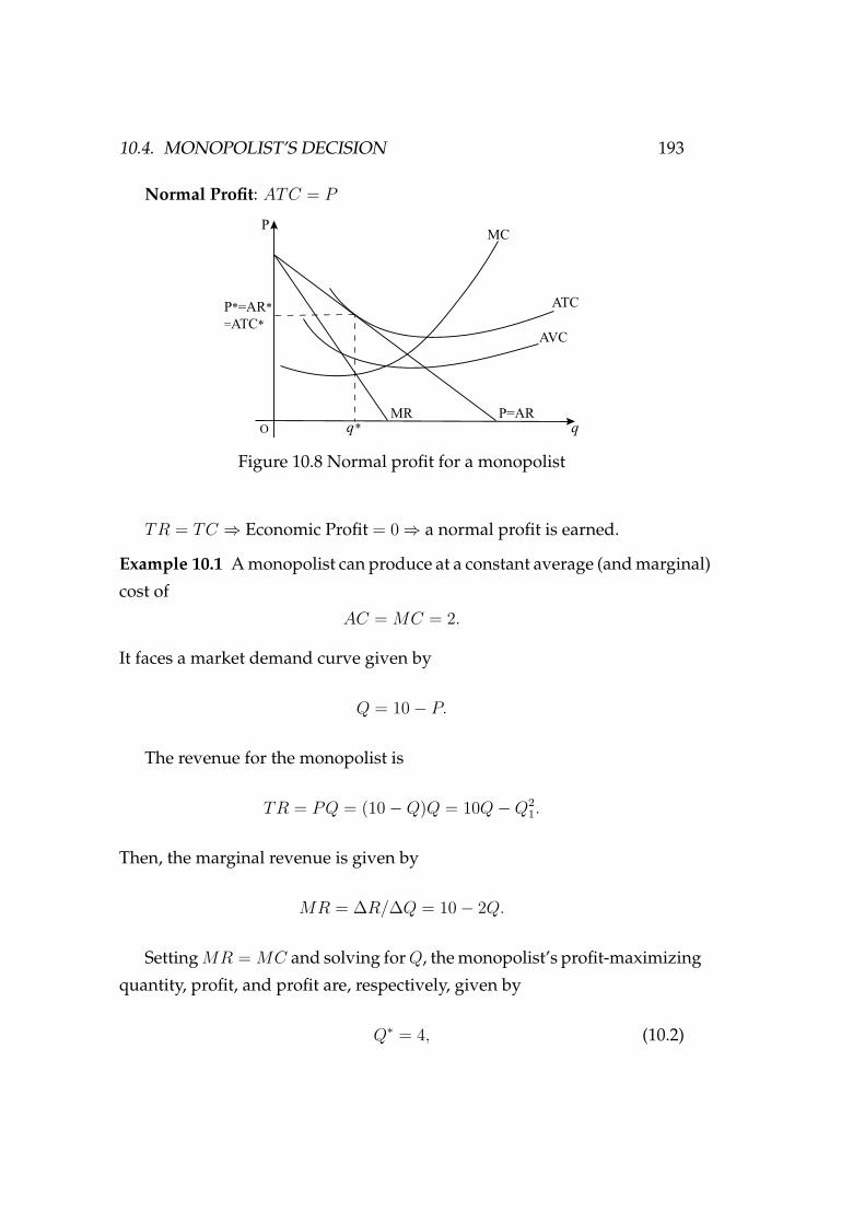
10.4. MONOPOLIST’S DECISION 193
Normal Profit: ATC = P
MC
P*=AR*
=ATC*
ATC
O
P
q*P=AR
AVC
MR
q
Figure 10.8 Normal profit for a monopolist
TR = TC ⇒ Economic Profit = 0 ⇒ a normal profit is earned.
Example 10.1 A monopolist can produce at a constant average (and marginal)
cost of
AC = MC = 2.
It faces a market demand curve given by
Q = 10 − P.
The revenue for the monopolist is
TR = PQ = (10 − Q)Q = 10Q − Q21.
Then, the marginal revenue is given by
MR = ∆R/∆Q = 10 − 2Q.
Setting MR = MC and solving for Q, the monopolist’s profit-maximizing
quantity, profit, and profit are, respectively, given by
Q∗ = 4, (10.2)

194 CHAPTER 10. MONOPOLY AND MONOPSONY
P ∗ = 6, (10.3)
and
π = TR − TC = Q∗(P ∗ − AC) = 16. (10.4)
Long-Run: a monopolist may earn positive economic profits in the
long run since barriers to competition prevent new firms from entering
the industry. (Under perfect competition this involved a shift in the sup-
ply curve which reduced the equilibrium price and eventually reduced
economic profits to zero.)
10.4.2 The Multiplant Firm
Suppose that a firm has two plants. What should its total output be, and
how much of that output should each plant produce? We can find the
answer intuitively in two steps.
• Step 1. Whatever the total output, it should be divided between the
two plants so that marginal cost is the same in each plant. Otherwise,
the firm could reduce its costs and increase its profit by reallocating
production.
• Step 2. We know that total output must be such that marginal rev-
enue equals marginal cost. Otherwise, the firm could increase its
profit by raising or lowering total output.
We can derive this result algebraically. Let Q1 and C1 be the output
and cost of production for Plant 1, Q2 and C2 be the output and cost of
production for Plant 2, and QT = Q1 + Q2 be total output. Then profit is
Π = PQT = PQ1 + PQ2 − c1(Q1) − c2(Q2),
and thus we have
MR = MC1 = MC2.

10.4. MONOPOLIST’S DECISION 195
Therefore, a firm with two plants maximizes profits by choosing output
levels Q1 and Q2 so that marginal revenue MR (which depends on total
output) equals marginal costs for each plant, MC1 and MC2, as depicted
in Figure 10.9.
$/Q
Quantity
D=AR
MR
MR*
P*
Q1 Q2 Q r
MC MC!
MC"
Figure 10.9 Producing with two plants
10.4.3 Relationships between MR, Price, and EPd
Since
MR = P + Q∆P
∆Q= P
(1 + Q
P× ∆P
∆Q
)= P
(1 + 1
EPd
),
we have
MR = P
(1 + 1
EPd
). (10.5)
Therefore, the less elastic its demand curve, the more monopoly power
a firm has. The ultimate determinant of monopoly power is therefore the
firm’s elasticity of demand.
We have the following typical cases:
1. When the elasticity of demand is infinity (a horizontal de-

196 CHAPTER 10. MONOPOLY AND MONOPSONY
mand curve), then MR = P :
MR = P(
1 − 1∞
)= P.
2. When demand is unit elastic (EPd = −1), then MR = 0:
MR = P(
1 − 11
)= 0.
3. When demand is elastic (|EPd | > 1), then MR > 0; e.g., let
EPd = −2:
MR = P(
1 − 12
)= 1
2P > 0.
4. When demand is inelastic (|EPd | < 1), then MR < 0; e.g., let
EPd = −1
2 :
MR = P
(1 − 1
1/2
)= P (1 − 2) = −P < 0.
There are three factors which determine a firm’s elasticity of demand:
• The elasticity of market demand. Because the firm’s own demand
will be at least as elastic as market demand, the elasticity of market
demand limits the potential for monopoly power.
• The number of firms in the market. If there are many firms, it is
unlikely that any one firm will be able to affect price significantly.
• The interaction among firms. Even if there are only few firms in
the market, each firm will be unable to profitably raise price very
much if the rivalry among them is aggressive, with each firm trying
to capture as much of the market as it can.
The Elasticity of Market Demand: If there is only one firm — a pure
monopolist — its demand curve is the market demand curve. In this case,
the firm’s degree of monopoly power depends completely on the elasticity
of market demand. When several firms compete with one another, the

10.4. MONOPOLIST’S DECISION 197
elasticity of market demand sets a lower limit on the magnitude of the
elasticity of demand for each firm.
A particular firm’s elasticity depends on how the firms compete with
one another, and the elasticity of market demand limits the potential monopoly
power of individual producers. Because the demand for oil is fairly in-
elastic (at least in the short run), OPEC could raise oil prices far above
marginal production cost during the 1970s and early 1980s. Because the
demands for such commodities as coffee, cocoa, tin, and copper are much
more elastic, attempts by producers to cartelize these markets and raise
prices have largely failed. In each case, the elasticity of market demand
limits the potential monopoly power of individual producers.
Example 10.2 (Elasticity of Demand for Soft Drinks) Soft drinks provide
a good example of the difference between a market elasticity of demand
and a firm’s elasticity of demand. In addition, soft drinks are importan-
t because their consumption has been linked to childhood obesity; there
could be health benefits from taxing them.
A recent review of statistical studies found that the market elasticity of
demand for soft drinks is between -0.8 and -1.0.6 That means that if all soft
drink producers increased the prices of all of their brands by 1 percent, the
quantity of soft drinks demanded would fall by 0.8 to 1.0 percent.
The demand for any individual soft drink, however, will be much more
elastic, because consumers can readily substitute one drink for another.
Although elasticities will differ across different brands, studies have shown
that the elasticity of demand for, say, Coca Cola is around -5. In other
words, if the price of Coke were increased by 1 percent but the prices of
all other soft drinks remained unchanged, the quantity of Coke demanded
would fall by about 5 percent.
Students-and business people-sometimes confuse the market elasticity
of demand with the firm (or brand) elasticity of demand. Make sure you
understand the difference.
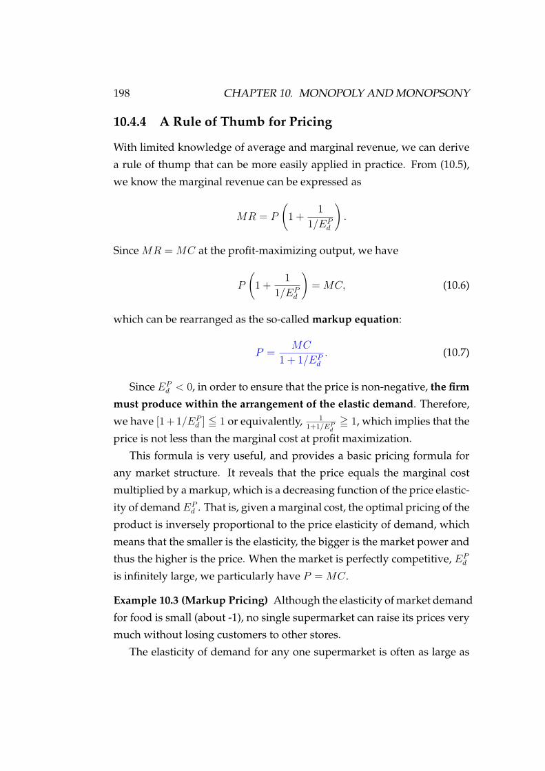
198 CHAPTER 10. MONOPOLY AND MONOPSONY
10.4.4 A Rule of Thumb for Pricing
With limited knowledge of average and marginal revenue, we can derive
a rule of thump that can be more easily applied in practice. From (10.5),
we know the marginal revenue can be expressed as
MR = P
(1 + 1
1/EPd
).
Since MR = MC at the profit-maximizing output, we have
P
(1 + 1
1/EPd
)= MC, (10.6)
which can be rearranged as the so-called markup equation:
P = MC
1 + 1/EPd
. (10.7)
Since EPd < 0, in order to ensure that the price is non-negative, the firm
must produce within the arrangement of the elastic demand. Therefore,
we have [1 + 1/EPd ] 5 1 or equivalently, 1
1+1/EPd= 1, which implies that the
price is not less than the marginal cost at profit maximization.
This formula is very useful, and provides a basic pricing formula for
any market structure. It reveals that the price equals the marginal cost
multiplied by a markup, which is a decreasing function of the price elastic-
ity of demand EPd . That is, given a marginal cost, the optimal pricing of the
product is inversely proportional to the price elasticity of demand, which
means that the smaller is the elasticity, the bigger is the market power and
thus the higher is the price. When the market is perfectly competitive, EPd
is infinitely large, we particularly have P = MC.
Example 10.3 (Markup Pricing) Although the elasticity of market demand
for food is small (about -1), no single supermarket can raise its prices very
much without losing customers to other stores.
The elasticity of demand for any one supermarket is often as large as

10.4. MONOPOLIST’S DECISION 199
-10. We then find that by markup equation (10.7),
P = MC/(1 − 0.1) = MC/(0.9) = (1.11)MC,
which is about 11 percent above marginal cost.
Small convenience stores typically charge higher prices because its cus-
tomers are generally less price sensitive. Because the elasticity of demand
for a convenience store is about -5, the markup equation (10.7) implies that
its prices should be about 25 percent above marginal cost. With designer
jeans, demand elasticities in the range of -2 to -3 are typical. This means
that price should be 50 to 100 percent higher than marginal cost.
Example 10.4 (Astra-Merck Prices Prilosec) In 1995, Prilosec, represent-
ed a new generation of antiulcer medication. Prilosec was based on a very
different biochemical mechanism and was much more effective than ear-
lier drugs. By 1996, it had become the best-selling drug in the world and
faced no major competitor.
Astra-Merck was pricing Prilosec at about $3.50 per daily dose. The
marginal cost of producing Prilosec is only about 30 to 40 cents per dose.
The price elasticity of demand should be in the range of roughly -1.0
to -1.2. Setting the price at a markup exceeding 400 percent over marginal
cost is consistent with our rule of thumb for pricing.
10.4.5 Measuring Monopoly Power
The important distinction between a perfectly competitive firm and a firm
with monopoly power: For the competitive firm, price equals marginal
cost; for the firm with monopoly power, price exceeds marginal cost.
Lerner Index of Monopoly Power: Measure of monopoly power cal-
culated as excess of price over marginal cost as a fraction of price:
L = P − MC
P,

200 CHAPTER 10. MONOPOLY AND MONOPSONY
which is also equal to minus the inverse of Epd by equation (10.6):
L = P − MC
P= − 1
Epd
.
$/Q
Quantity
AR
MR
P*
Q*
P*=MC MC
$/Q
Quantity
AR
MR
P*
MC
Q*
P*=MC
(a) (b)
Figure 10.10 Elasticity of demand and price markup
Thus, if the firm’s demand is elastic, as in (a) of Figure 10.10, the markup
is small and the firm has little monopoly power. The opposite is true if de-
mand is relatively inelastic, as in (b) of Figure 10.10.
10.5 Further Implications of Monopoly Analysis
Monopoly Has No Supply Curve
Under perfect competition we noticed that at any given price there is a
unique quantity of output that the firm is willing to supply. Conversely,
at any given output level there is a unique price that makes the firm be
willing to supply that output level. This relationship does not exist for the
case of a monopolist, and hence monopoly has no supply curve. The rea-
son is that a monopolist’s output decision depends not only on marginal
cost but also on the demand curve.

10.6. MONOPOLY VERSUS PERFECT COMPETITION 201
Consider two possible demand curves below in Figure 10.11: MR1 and
MR2 intersect MC at the same point:
• If demand curve is D1, then price is P1.
• If demand curve is D2, then price is P2.
MC
P�
P
q* MR� q
D� D
MR
P
Figure 10.11 No supply curve: A change of demand only changes the pricecharged
Thus, a MC curve cannot be supply curve for a monopolist. Therefore,
a monopoly has no supply curve. In other words, there is no one-to-one
relationship between price and the quantity produced. As a result, shifts
in demand do not trace out the series of prices and quantities that corre-
spond to a competitive supply curve. Instead, shifts in demand can lead
to changes in price with no change in output, changes in output with no
change in price, or changes in both price and output.
However, the absence of a monopoly supply curve does not mean that
we are unable to analyze the output choice of a monopoly.
10.6 Monopoly versus Perfect Competition
Perfectly Competitive Industry: S = ∑i MCi, S = D ⇒ P c, qc.

202 CHAPTER 10. MONOPOLY AND MONOPSONY
SP
qc q
D
Pc
Figure 10.12 Market equilibrium under perfect competition
MC
P
qc q
Pc
MR D
Pm
qm
Figure 10.13 Market equilibrium under monopoly
Monopoly (a single firm takes over all firms): MR = MC ⇒ qm, P m.
Therefore, when an industry is a monopoly consumers pay a higher
price and receive less than would be the case under perfect competition.
10.7 The Social Cost of Monopoly Power
10.7.1 Income Distribution Problem
If a competitive industry becomes a monopoly, there will be a change in
the distribution of real income among members of society. The monop-
olist will gain. Consumers will lose because of a higher price they pay.

10.7. THE SOCIAL COST OF MONOPOLY POWER 203
The higher price reduces the real purchasing power, or real income, of the
consumers. Thus, by changing a price above average cost, the monopo-
list gains at the expense of the consumers–a redistribution of income from
consumers to the owners of the monopoly.
10.7.2 Inefficient Allocations
Monopoly has another effect that involves a net loss in welfare because
it leads to an inefficient allocation. Economists refer to this net loss as a
social cost of monopoly.
Quantity
AR
Pc
Pm
Q cQm
Deadweight
Loss
A
C
B
$/Q
MC
MR
Lost Consumer Surplus
Figure 10.14 Deadweight Loss form Monopoly Power
The shaded rectangle and triangles in Figure 10.14 show changes in
consumer and producer surplus when moving from competitive price and
quantity, Pc and Qc, to a monopolist’s price and quantity, Pm and Qm.
Because of the higher price, consumers lose A + B and producer gains
A − C. The deadweight loss is B + C.
Price Regulation
How can we solve the inefficiency issue of monopoly? One way is to reg-
ular the price, especially to the competitive price.

204 CHAPTER 10. MONOPOLY AND MONOPSONY
If left alone, a monopolist produces Qm and charges Pm as shown in
10.15. When the government imposes a price ceiling of P1 the firm’s aver-
age and marginal revenue are constant and equal to P1 for output levels
up to Q1. For larger output levels, the original average and marginal rev-
enue curves apply. The new marginal revenue curve is, therefore, the dark
purple line, which intersects the marginal cost curve at Q1.
Figure 10.15 Price Regulation
When price is lowered to Pc, at the point where marginal cost intersects
average revenue, output increases to its maximum Qc. This is the output
that would be produced by a competitive industry.
Lowering price further, to P3, reduces output to Q3 and causes a short-
age, Q′3 − Q3.
10.8 Benefits of Monopoly: Corporate Innovation
Although social costs of monopoly, it is not without certain merit. The
most merit of monopoly is that it provides strong incentives for the firm
to innovate continuously to conduct research and develop new products.

10.9. MONOPSONY 205
Corporate innovation leads to monopoly profits, and considerable prof-
its will attract other firms to enter and compete again. In this way, market
competition leads to the decrease of profits and firms obtain monopoly
profits through innovation, which forms a repeated cycle of competition-
innovation-monopoly-competition. In this cycle, market competition pro-
duces market equilibrium, while innovation disrupts this equilibrium. This
repeated game in the market motivates firms to constantly pursue innova-
tion. Through this repeated game process, the market economy maintains
long-term vitality, increases social welfare and promotes economic devel-
opment, revealing the unique beauty and power of the market system.
Of course, in order to encourage innovation, the government should e-
nact intellectual property protection laws. At the same time, to encourage
competition and form externalities of technology innovation, the protec-
tion given by anti-monopoly laws and intellectual property rights legisla-
tion should not be permanent, but rather for a limited time, in case fixed
or permanent oligopolies and monopolies may appear.
Thus, competition and monopoly are two sides of the same entity, like
supply and demand, the two of which can become an awe-inspiring di-
alectical unity of opposites under market forces, showing the beauty and
power of the market system.
10.9 Monopsony
Monopsony power: Buyer’s ability to affect the price of a good.
Oligopsony: Market with only a few buyers.
Marginal value (MV): Additional benefit derived from purchasing one
more unit of a good.
Marginal expenditure (ME): Additional cost of buying one more unit
of a good.
Average expenditure (AE): Price paid per unit of a good.

206 CHAPTER 10. MONOPOLY AND MONOPSONY
10.9.1 Competitive Buyer Compared to Competitive Seller
$/Q
ME=AE
D=MV
Quantity
P*
$/Q
MC
AR=MR
Quantity
P*
Q* Q*
(a) (b)
Figure 10.16 Competitive buyer compared to competitive seller
In Figure 10.16.(a), the competitive buyer takes price P* as given, hence
marginal expenditure and average expenditure are constant and equal:
ME = AV.
Quantity purchased is found by price equating marginal value (demand).
In Figure 10.16.(b), the competitive seller also takes price as given.
Marginal revenue and average revenue are constant and equal; quantity
sold is found by equating price to marginal cost.
10.9.2 Monopsony Buyer
The market supply curve is monopsonist’s average expenditure curve AE.
Because average expenditure is rising, marginal expenditure lies above it.
In Figure 10.17, the monopsonist purchases quantity Q∗m, where marginal
expenditure and marginal value (i.e., demand) intersect.
The price paid per unit P ∗m is then found from the average expenditure
(i.e., supply) curve. In a competitive market, price and quantity, Pc and Qc,
are both higher. They are found at the point where average expenditure

10.9. MONOPSONY 207
(supply) and marginal value (demand) intersect.
$/Q
MV
S=AE
Quantity
P*
Q*
ME
m Qc
m
Pc
Figure 10.17 Monopsonist buyer
Monopoly and Monopsony
$/Q
Quantity
P*
Q*
$/Q
Quantity
AR
MR
P*
MC
Q*
(a) (b)
Pc
Qc
Pc
Qc
MV
ME
S=AE
Figure 10.18 Monopoly and Monopsony
These diagrams show the close analogy between monopoly and monop-
sony.
(a) The monopolist produces where marginal revenue inter-
sects marginal cost. Average revenue (i.e. demand) exceeds
marginal revenue, so that price exceeds marginal cost.

208 CHAPTER 10. MONOPOLY AND MONOPSONY
(b) The monopsonist purchases up to the point where marginal
expenditure intersects marginal value.
Marginal expenditure exceeds average expenditure (i.e., supply), so
that marginal value exceeds price.
10.10 Monopsony Power
10.10.1 Monopsony Power: Elastic versus Inelastic Supply
Monopsony power depends on the elasticity of supply. When supply is
elastic, as in Figure 10.19.(a), marginal expenditure and average expen-
diture do not differ by much, so price is close to what it would be in a
competitive market.
The opposite is true when supply is inelastic, as in Figure 10.19.(b).
$/Q
Quantity
P*
Q*
$/Q
Quantity
MV
P*
Q*
(a) (b)
MV
ME
S=AE
MV-P*
ME
S=AE
MV-P*
Figure 10.19 Monopsony power: elastic versus inelastic supply
10.10.2 Sources of Monopsony Power
• Elasticity of market supply: If only one buyer is in the market-a pure
monopsonist-its monopsony power is completely determined by the

10.10. MONOPSONY POWER 209
elasticity of market supply. If supply is highly elastic, monopsony
power is small and there is little gain in being the only buyer.
• Number of buyers: When the number of buyers is very large, no
single buyer can have much influence over price. Thus each buyer
faces an extremely elastic supply curve, so that the market is almost
completely competitive.
• Interaction among buyers: If buyers in a market compete aggres-
sively, they will bid up the price close to their marginal value of the
product, and will thus have little monopsony power. On the oth-
er hand, if those buyers compete less aggressively, or even collude,
prices will not be bid up very much, and the degree of monopsony
power might be nearly as high as if there were only one buyer.
10.10.3 The Social Costs of Monopsony Power
Quantity
S=AE
MV
P0
Pm
Q cQm
Deadweight Loss
A C
B
C
$/Q ME
Figure 10.20 Monopsony power: elastic versus inelastic supply
The shaded rectangle and triangles in Figure 10.20 show changes in buyer
and seller surplus when moving from competitive price and quantity, Pc

210 CHAPTER 10. MONOPOLY AND MONOPSONY
and Qc, to the monopsonist’s price and quantity, Pm and Qm.
Because both price and quantity are lower, there is an increase in buyer
(consumer) surplus given by A − B. Producer surplus falls by A + C, so
there is a deadweight loss given by triangles B and C.
10.10.4 Bilateral Monopsony
Bilateral monopoly: Market with only one seller and one buyer.
It is difficult to predict the price and quantity in a bilateral monopoly.
Both the buyer and the seller are in a bargaining situation.
Bilateral monopoly is rare. Although bargaining may still be involved,
we can apply a rough principle here: Monopsony power and monopoly
power will tend to counteract each other. In other words, the monopsony
power of buyers will reduce the effective monopoly power of sellers, and
vice versa.
This tendency does not mean that the market will end up looking per-
fectly competitive, but in general, monopsony power will push price clos-
er to marginal cost, and monopoly power will push price closer to marginal
value.
10.11 Limiting Market Power: The Antitrust Laws
Excessive market power harms potential purchasers and raises problems
of equity and fairness. In addition, market power reduces output, which
leads to a deadweight loss.
In theory, a firm’s excess profits could be taxed away, but redistribution
of the firm’s profits is often impractical.
To limit the market power of a natural monopoly, such as an electric
utility company, direct price regulation is the answer.
Antitrust laws: Rules and regulations prohibiting actions that restrain,
or are likely to restrain, competition. That is, it is designed to promote to

10.11. LIMITING MARKET POWER: THE ANTITRUST LAWS 211
competition.
It is important to stress that, while there are limitations (such as collud-
ing with other firms), in general, it is not illegal to be a monopolist or to
have market power. On the contrary, we have seen that patent and copy-
right laws protect the monopoly positions of firms that developed unique
innovations.
Restricting What Firms Can Do
Parallel conduct: Form of implicit collusion in which one firm consistently
follows actions of another.
Predatory pricing: Practice of pricing to drive current competitors out
of business and to discourage new entrants in a market so that a firm can
enjoy higher future profits.
Enforcement of the Antitrust Laws
The antitrust laws are enforced in three ways:
• Through the Antitrust Division of the Department of Justice.
• Through the administrative procedures of the Federal Trade Com-
mission.
• Through private proceedings.
Example 10.5 (Microsoft) Over the past three decades Microsoft has dom-
inated the software market for personal computers, having maintained
over a 90-percent market share for operating systems and for office suites.
In 1998, the Antitrust Division of the U.S. DOJ filed suit, claiming that
Microsoft had illegally bundled its Internet browser with its operating sys-
tem for the purpose of maintaining its dominant operating system monopoly.
The court found that Microsoft did have monopoly power in the market
for PC operating systems, which it had maintained illegally in violation of
Section 2 of the Sherman Act.

212 CHAPTER 10. MONOPOLY AND MONOPSONY
In 2004, the European Commission claimed that by bundling the Win-
dows Media Player with the operating system, Microsoft would monop-
olize the market for media players. Microsoft agreed to offer customers a
choice of browsers when first booting up their new operating system, and
the case came to a close in 2012.
By 2016, the locus of competition had moved to the smartphone in-
dustry, where Microsoft faces strong competition from Google’s (Android)
and Apple’s (iOS) operating systems.

Chapter 11
Pricing with Market Power
11.1 Capturing Consumer Surplus
The pricing of monopoly discussed in previous chapter is uniform price,
but in reality, firms usually adopt differential pricing. The premise of d-
ifferential pricing is that the purchase of the demander will generate con-
sumer surplus. A monopolist may obtain some, or even all, of the con-
sumer surplus through price discrimination.
Price discrimination: Selling the same good or service at different
prices to different buyers.
Monopolists use price discrimination to realize greater profits. They
have ability to do this since they are the only supplier of a good. E.g.,
• movie theaters charge different prices for children and adults.
• utility companies charge different rates for businesses and residences.
• senior citizens pay a lower fare for bus ride.
Conditions which aid price discrimination:
• resale not possible;
• must be able to segment the market by classifying buyers in separate,
identifiable groups (say, by showing ID);
213

214 CHAPTER 11. PRICING WITH MARKET POWER
• monopoly control;
• different demand elasticities: E.g., Mr. A’s demand is less elastic,
and Mr. B’s demand is more elastic. Monopolists can increase TR by
increasing price for Mr. A while decreasing price for Mr. B.
There are many broadly adopted forms of price discrimination in prac-
tice.
11.2 First-Degree Price Discrimination
Reservation price: Maximum price that a customer is willing to pay for a
good.
First degree price discrimination: Practice of charging each customer
her reservation price.
11.2.1 Capturing Consumer Surplus by Perfect Price Dis-
crimination
Assume below that MC = ATC which is constant.
MC=ATC
P
qd
q
MR D
Pm
qm
a b
cd
e
Figure 11.1 Market equilibrium under perfect price discrimination

11.2. FIRST-DEGREE PRICE DISCRIMINATION 215
If the same price is charged for all goods, then profit is maximized at
qm, sold at pm. Profit = area abcd.
If the monopolist uses perfect price discrimination to charge the max-
imum price buyers are willing to pay for each additional unit, then the
profit expands to the area between the demand curve and the marginal
cost curve.
11.2.2 Capturing Consumer Surplus by Imperfect Price Dis-
crimination
Firms usually do not know the reservation price of every consumer, but
sometimes reservation prices can be roughly identified. In Figure 11.2,
six different prices are charged. The firm earns higher profits, but some
consumers may also benefit. With a single price P ∗4 , there are fewer con-
sumers. The consumers who now pay P5 or P6 enjoy a surplus.
$/Q
Quantity
D
MR
P*MC
4
P5P6
P3
P2
P1
Figure 11.2 First-degree price discrimination in practice
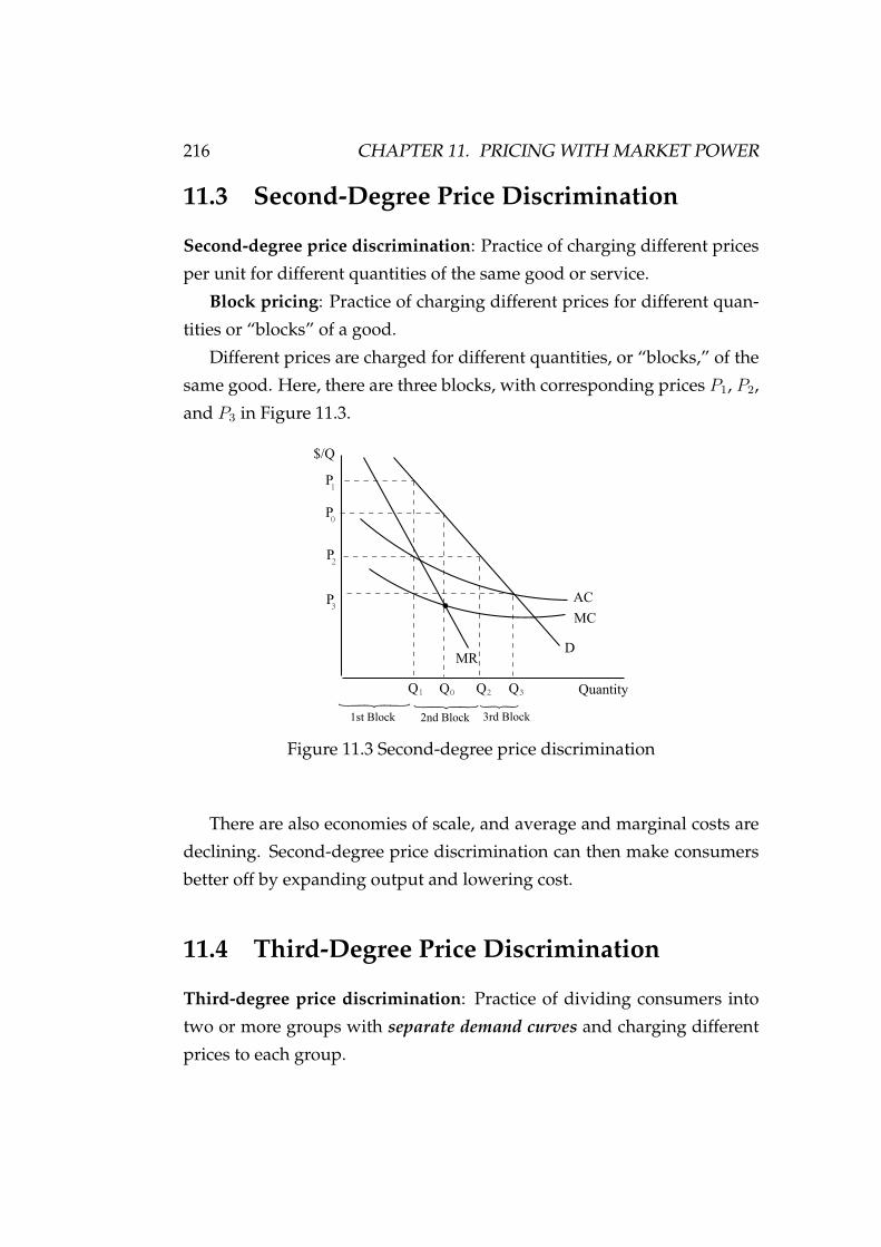
216 CHAPTER 11. PRICING WITH MARKET POWER
11.3 Second-Degree Price Discrimination
Second-degree price discrimination: Practice of charging different prices
per unit for different quantities of the same good or service.
Block pricing: Practice of charging different prices for different quan-
tities or “blocks” of a good.
Different prices are charged for different quantities, or “blocks,” of the
same good. Here, there are three blocks, with corresponding prices P1, P2,
and P3 in Figure 11.3.
$/Q
Quantity
AC
MR
P
MC
2
P3
P0
P1
D
Q1 Q0 Q2 Q3{ { {
1st Block 2nd Block 3rd Block
Figure 11.3 Second-degree price discrimination
There are also economies of scale, and average and marginal costs are
declining. Second-degree price discrimination can then make consumers
better off by expanding output and lowering cost.
11.4 Third-Degree Price Discrimination
Third-degree price discrimination: Practice of dividing consumers into
two or more groups with separate demand curves and charging different
prices to each group.

11.4. THIRD-DEGREE PRICE DISCRIMINATION 217
Creating Consumer Groups
If third-degree price discrimination is feasible, how should the firm decide
what price to charge each group of consumers?
We know that however much is produced, total output should be di-
vided between the groups of customers so that marginal revenues for each
group are equal. We know that total output must be such that the marginal
revenue for each group of consumers is equal to the marginal cost of pro-
duction.
Let P1 be the price charged to the first group of consumers, P2 the price
charged to the second group, and C(QT ) the total cost of producing output
QT = Q1 + Q2. Total profit is then
Π = P1Q1 + P2Q2 − C(QT )
and thus
MR1 = MR2 = MC.
Therefore, from
MR = P (1 + 1/Epd),
the relative prices are given by
P1
P2= (1 + 1/E2)
(1 + 1/E1).
Consider Figure 11.4. Consumers are divided into two groups, with
separate demand curves for each group. The optimal prices and quantities
are such that the marginal revenue from each group is the same and equal
to marginal cost.
Here group 1, with demand curve D1, is charged P1, and group 2, with
the more elastic demand curve D2, is charged the lower price P2. Marginal
cost depends on the total quantity produced QT . Note that Q1 and Q2 are
chosen so that MR1 = MR2 = MC.

218 CHAPTER 11. PRICING WITH MARKET POWER
Quantity
D = AR
P2
P1
Q2Q1
A
$/Q
MC
MRT
MR2
2 2
D= AR1 1MR1
QT
Figure 11.4 Third-degree price discrimination
Example 11.1 (The Economics of Coupons and Rebates) Coupons provide
a means of price discrimination.
Price Elasticity Price ElasticityProduct Nonusers Users
Toilet -0.60 -0.66Stuffing/dressing -0.71 -0.96
Shampoo -0.84 -1.04Cooking/salad oil -1.22 -1.32Dry mix dinners -0.88 -1.09
Cake mix -0.21 -0.43Cat food -0.49 -1.13
Frozen entrees -0.60 -0.95Gelatin -0.97 -1.25
Spaghetti sauce -1.65 -1.81Creme rinse/conditioner -0.82 -1.12
Soups -1.05 -1.22Hot dogs -0.59 -0.77
Table 11.1: Price elasticity of demand for users versus nonusers of coupons

11.5. THE TWO-PART TARIFF 219
Example 11.2 (Airline Fares) Travelers are often amazed at the variety of
fares available for round-trip flights.
Fare Category Fare Category Fare CategoryElasticity First Class Unrestricted Coach Discouted
Price -0.3 -0.4 -0.9Income 1.2 1.2 1.8
Table 11.2: Elasticities of demand for air travel
Recently, for example, the first-class fare for round-trip flights from
New York to Los Angeles was above $2000; the regular (unrestricted) e-
conomy fare was about $1000, and special discount fares (often requiring
the purchase of a ticket two weeks in advance and/or a Saturday night
stay over) could be bought for as little as $200. These fares provide a
profitable form of price discrimination. The gains from discriminating are
large because different types of customers, with very different elasticities
of demand, purchase these different types of tickets. Airline price discrim-
ination has become increasingly sophisticated. A wide variety of fares is
available.
11.5 The Two-Part Tariff
Two-part tariff: Form of pricing in which consumers are charged both an
entry fee and a usage fee.
It is also commonly used in practice.
11.5.1 Two-Part Tariff with a Single Consumer
The consumer has demand curve D as shown in Figure 11.5. The firm
maximizes profit by setting usage fee P equal to marginal cost and entry
fee T ∗ equal to the entire surplus of the consumer.

220 CHAPTER 11. PRICING WITH MARKET POWER
$/Q
MC
D
Quantity
P*
T
Figure 11.5 Two-Part Tariff with a Single Consumer
11.5.2 Two-Part Tariff with Two Consumer
The profit-maximizing usage fee P ∗ will exceed marginal cost. The entry
fee T ∗ is equal to the surplus of the consumer with the smaller demand.
The resulting profit is 2T ∗ + (P ∗ − MC)(Q1 + Q2). Note that this profit
is larger than twice the area of triangle ABC as shown in Figure 11.6.
$/Q
MC
D�
Quantity
P*
T*
D
BC
Q�Q
A
Figure 11.6 Two-Part Tariff with a Single Consumer
Example 11.3 (Pricing Cellular Phone Service) Cellular phone service has

11.5. THE TWO-PART TARIFF 221
traditionally been priced using a two-part tariff: a monthly access fee,
which includes some amount of free “anytime” minutes, plus a per-minute
charge for additional minutes.
Offering different plans allowed companies to combine third-degree
price discrimination with the two-part tariff.
Today, most consumers use their phone not just to make or receive calls
but also to surf the Web, read email, and so on. They separate themselves
into groups based on their expected data usage, with each group choosing
a different plan. Cellular providers have learned that the most profitable
way to price their service is to combine price discrimination with a two-
part tariff.
Data Usage Monthly Price Monthly Access Charge Overage FeeA. Verizon A. Verizon A. Verizon A. Verizon
1 GB $30 $ 20 $ 15/GB3GB $45 $ 20 $ 15/GB6GB $60 $ 20 $ 15/GB
12GB $80 $ 20 $ 15/GB18GB $100 $ 20 $ 15/GB
B. Sprint B. Sprint B. Sprint B. Sprint1GB $20 $ 45 $ none3GB $30 $ 45 $ none6GB $45 $ 45 $ none
12GB $60 $ 45 $ none24GB $80 $ 45 $ none
C. AT&T C. AT&T C. AT&T C. AT&T2GB $30 $ 25 $ 15/GB5GB $50 $ 25 $ 15/GB
15GB $100 $ 15 $ 15/GB20GB $140 $ 15 $ 15/GB25GB $175 $ 15 $ 15/GB30GB $225 $ 15 $ 15/GB
Table 11.3: Cellular data plans (2016)

222 CHAPTER 11. PRICING WITH MARKET POWER
11.6 Intertemporal Price Discrimination and Peak-
Load Pricing
Intertemporal price discrimination: Practice of separating consumers with
different demand functions into different groups by charging different
prices at different points in time.
Consumers are divided into groups by changing the price over time.
Initially, the price is high. The firm captures surplus from consumers who
have a high demand for the good and who are unwilling to wait to buy it.
Later the price is reduced to appeal to the mass market.
Example 11.4 (How to Price a Best-selling Novel) Publishing both hard-
bound and paperback editions of a book allows publishers to price dis-
criminate.
Some consumers want to buy a new bestseller as soon as it is released,
even if the price is $25. Other consumers, however, will wait a year until
the book is available in paperback for $10.
The key is to divide consumers into two groups, so that those who are
willing to pay a high price do so and only those unwilling to pay a high
price wait and buy the paperback.
It is clear, however, that those consumers willing to wait for the paper-
back edition have demands that are far more elastic than those of biblio-
philes. It is not surprising, then, that paperback editions sell for so much
less than hardbacks.
Peak-load pricing: Practice of charging higher prices during peak periods
when capacity constraints cause marginal costs to be high.
Demands for some goods and services increase sharply during partic-
ular times of the day or year.
Charging a higher price during the peak periods is more profitable for
the firm than charging a single price at all times.
It is also more efficient because marginal cost is higher during peak
periods.

11.7. BUNDLING 223
11.7 Bundling
Bundling: Practice of selling two or more products as a package.
To see how a film company can use customer heterogeneity to its ad-
vantage, suppose that there are two movie theaters and that their reserva-
tion prices for the two films are as follows:
Gone with the Wind Getting Gertie’s GarterTheater A $12,000 $3,000Theater B $10,000 $4,000
Table 11.4: Selling two films as a package
If the films are rented separately, the maximum price that could be
charged for Wind is $10,000 because charging more would exclude The-
ater B. Similarly, the maximum price that could be charged for Gertie is
$3000. The total revenue is $26,000.
But suppose the films are bundled. Theater A values the pair of films at
$15,000 ($12,000 + $3000), and Theater B values the pair at $14,000 ($10,000
+ $4000). Therefore, we can charge each theater $14,000 for the pair of films
and earn a total revenue of $28,000.
Why is bundling more profitable than selling the films separately? Be-
cause the relative valuations of the two films are reversed. The demands
are negatively correlated-the customer willing to pay the most for Wind is
willing to pay the least for Gertie.
Suppose demands were positively correlated-that is, Theater A would
pay more for both films:
Gone with the Wind Getting Gertie’s GarterTheater A $12,000 $4,000Theater B $10,000 $3,000
Table 11.5: Selling two films as a package

224 CHAPTER 11. PRICING WITH MARKET POWER
If we bundled the films, the maximum price that could be charged for
the package is $13,000, yielding a total revenue of $26,000, the same as by
renting the films separately.

Chapter 12
Monopolistic Competition and
Oligopoly
Competition and monopoly lie at opposite ends of the market spectrum.
While competition is characterized by many firms, unrestricted entry, and
homogeneous products, a monopoly is the sole producer of a product with
no close substitutes. Falling between competition and monopoly are two
other types of market structures, monopolistic competition and oligopoly,
which describe the major part of remaining firms. In substance, monop-
olistic competition is closer to competition; it has many firms and un-
restricted entry or exit, like the competitive model, but its products are
differentiated. Oligopoly, on the other hand, is more like monopoly; it
is characterized by a small number of large firms producing either a ho-
mogeneous product like steel, or differentiated products like automobiles,
and acting to each other in their actions. In the following, we will exam-
ine some of these models, noting the similarities as well as the differences
between these models.
225
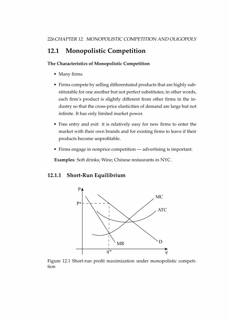
226CHAPTER 12. MONOPOLISTIC COMPETITION AND OLIGOPOLY
12.1 Monopolistic Competition
The Characteristics of Monopolistic Competition
• Many firms.
• Firms compete by selling differentiated products that are highly sub-
stitutable for one another but not perfect substitutes; in other words,
each firm’s product is slightly different from other firms in the in-
dustry so that the cross-price elasticities of demand are large but not
infinite. It has only limited market power.
• Free entry and exit: it is relatively easy for new firms to enter the
market with their own brands and for existing firms to leave if their
products become unprofitable.
• Firms engage in nonprice competition — advertising is important.
Examples: Soft drinks; Wine; Chinese restaurants in NYC.
12.1.1 Short-Run Equilibrium
P
q
MRD
P*
q*
MC
ATC
Figure 12.1 Short-run profit maximization under monopolistic competi-tion

12.1. MONOPOLISTIC COMPETITION 227
The same as monopolist. Because the firm is the only producer of its brand,
it faces a downward-sloping demand curve. Price exceeds marginal cost
and the firm has monopoly power. E.g., profit maximization.
12.1.2 Long-Run Equilibrium
Recall that a monopolist can earn positive economic profits in the long
run. The above equilibrium could represent a monopolist’s LR equilibri-
um. This does not hold for a monopolistically competitive firm as there
are no barriers to entry.
Entry Eliminates Profits:
P
q
MR1
D
P*
q*
MC
ATC
MR2 D!
1q*
2
1
P*2
Figure 12.2 Entry eliminates profits under monopolistic competition
In the long run firms will enter the industry. Industry demand must be
divided between more firms ⇒ demand for each firm is reduced. (D and
MR shift to the left until profits are normal as depicted in Figure 12.2.) The
long-run equilibrium is given by (p2, q∗2)
Exit Eliminates Losses:
As firms exit, the market demand is spread over fewer firms ⇒ de-
mand for each remaining firm’s output increases ⇒ D & MR shift to the
right as depicted in Figure 12.3.

228CHAPTER 12. MONOPOLISTIC COMPETITION AND OLIGOPOLY
P
q
MR2
D
P
q*
MCATC
MR1 D!
1q*
2
1
P2
Figure 12.3 Exit eliminates losses under monopolistic competition
12.1.3 Monopolistic Competition and Economic Efficiency
Under perfect competition, price equals marginal cost. The demand curve
facing the firm is horizontal, so the zero-profit point occurs at the point of
minimum average cost.
However, under monopolistic competition, the demand curve is downward-
sloping, so the zero profit point is to the left of the point of minimum av-
erage cost. So price exceeds marginal cost. Thus there is a deadweight
loss, the same as the monopoly.
Is monopolistic competition then a socially undesirable market struc-
ture that should be regulated? The answer — for two reasons — is proba-
bly no:
(1) In most monopolistically competitive markets, monopoly
power is small. Usually enough firms compete, with brand-
s that are sufficiently substitutable, so that no single firm
has much monopoly power. Any resulting deadweight loss
will therefore be small. And because firms’ demand curves

12.2. OLIGOPOLY 229
will be fairly elastic, average cost will be close to the mini-
mum.
(2) Any inefficiency must be balanced against an importan-
t benefit from monopolistic competition: product diversi-
ty. Most consumers value the ability to choose among a
wide variety of competing products and brands that differ
in various ways. The gains from product diversity can be
large and may easily outweigh the inefficiency costs result-
ing from downward-sloping demand curves.
Example 12.1 (Monopolistic Competition for Soft Drinks and Coffee) The
markets for soft drinks and coffee illustrate the characteristics of monopo-
listic competition. Each market has a variety of brands that differ slightly
but are close substitutes for one another.
Brand Elasticity of DemandColas:
RC Cola -2.4Coke -5.2 to -5.7
Grand Coffee:Folgers -6.4Maxell house -8.2Chock Full o’ Nuts -3.6
Table 12.1: Elasticity of demand for Colas and Coffee
With the exception of RC Cola and Chock Full o’ Nuts, all the colas and
coffees are quite price elastic. With elasticities on the order of -4 to -8, each
brand has only limited monopoly power. This is typical of monopolistic
competition.
12.2 Oligopoly
Oligopoly is an industry characterized by a few large firms producing

230CHAPTER 12. MONOPOLISTIC COMPETITION AND OLIGOPOLY
most of or all of the output of some product, and reacting to each other in
pricing and output decisions.
Characteristics of Oligopoly:
a) Economies of scale: It only takes a few firms of size q to
supply the whole market. Scale economies may make it un-
profitable for more than a few firms to coexist in the mar-
ket; patents or access to a technology may exclude potential
competitors; and the need to spend money for name recog-
nition and market reputation may discourage entry by new
firms. These are “natural” entry barriers — they are basic to
the structure of the particular market. In addition, incum-
bent firms may take strategic actions to deter entry. Man-
aging an oligopolistic firm is complicated because pricing,
output, advertising, and investment decisions involve im-
portant strategic considerations, which can be highly com-
plex.
P
q
Market Demand
Q
P
Figure 12.4 Downward-sloping demand curve under oligopoly
b) Mutual interdependence among firms - since there are on-
ly a few firms in the market each firm must react to other
firms’ actions.

12.2. OLIGOPOLY 231
c) Nonprice competition and price rigidity. Price war is last
alternative (fear of lowering profits). Competition relies on
advertising and product differentiation.
d) Temptation for firms to collude in setting prices. Firms
may want to maximize collective profits. This is illegal in
the U.S.
e) Incentive for firms to merge. There is “perfect collusion”
when the industry becomes a monopoly.
f) Substantial barriers to entry - such as
(i) economies of scale
P
Q
D
P!
ATC
D!
P
D
ATC
o
Figure 12.5 Individual demand and market demand under oligopoly
• D: demand faced by the first firm with no
competitors.
• D1: demand faced by the first firm with
one competitor.
• D2: demand faced by the competitor (D =D1 + D2).
• ATC: the same for both firms, with economies
of scale.

232CHAPTER 12. MONOPOLISTIC COMPETITION AND OLIGOPOLY
Strategy for firm 1:
Charge a price below P2 and above P1. The poten-
tial loss of firm 2 will prevent it from entering
the market.
Note: ATC ′ ⇒ the 1st firm cannot use price to
keep the 2nd firm out of the market.
(ii) cost structure
P
q
P
ATC
D =D!
P2
D
ATC!
Figure 12.6 Oligopolistic firms with heterogeneous cost structures
Assume:
• firm 2 steals half of the market.
• costs for new firms are higher (ATC2 >
ATC1).
Strategy for firm 1:
The first firm can keep the 2nd firm out by choos-
ing a price between P1 and P2. P2 is referred
to as the limit price because any price greater
than this will induce entry.
Therefore, in oligopolistic markets, the products may or may not be

12.2. OLIGOPOLY 233
differentiated. What matters is account for most or all of total produc-
tion. In some oligopolistic that only a few firms markets, some or all firms
earn substantial profits over the long run because barriers to entry make
it difficult or impossible for new firms to enter. Oligopoly is a prevalen-
t form of market structure. Examples of oligopolistic industries include
automobiles, steel, aluminum, petrochemicals, electrical equipment, and
computers.
In an oligopolistic market, however, a firm sets price or output based
partly on strategic considerations regarding the behavior of its competi-
tors. With some modification, the underlying principle to describe an
equilibrium when firms make decisions that explicitly take each other’s
behavior into account is the same as the equilibrium in competitive and
monopolistic markets: When a market is in equilibrium, firms are doing
the best they can and have no reason to change their price or output.
Game theory will paly in important role in studying the behavior of
oligopolistic firms.
Game theory: Situation in which players (participants) make strategic
decisions that take into account each other’s actions and responses.
It can provide us with a way to examine the nature of interdependence
among rival firms and to understand the role of uncertainty in their pric-
ing and output decisions.
A game is described by the number of players, the set of strategies, the
payoffs of players, the forms of game (static or dynamic), and the infor-
mation (complete or incomplete information) available to the players.
Payoff: Value associated with a possible outcome.
Strategy: Rule or plan of action for playing a game.
Optimal strategy: Strategy that maximizes a player’s expected payoff.
It is essential to understand your opponent’s point of view and to de-
duce his or her likely responses to your actions.
The basic and most common used solution concept of a game is Nash

234CHAPTER 12. MONOPOLISTIC COMPETITION AND OLIGOPOLY
equilibrium, introduced by John Nash, a Nobel Laureate in Economics and
Abel Prize winner, who inspired the movie “A beautiful Mind”.
Nash equilibrium: A profile of strategies or actions in which each firm
does the best it can given its competitors’ actions. In other words, in Nash
Equilibrium, each firm is doing the best given what its competitors are
doing, and thus has no incentive to deviate from the equilibrium strategy.
Therefore, at a Nash equilibrium, each firm will no longer adjust his
own strategy given his rational expectation on the opponents’ strategy
profile. Thus, an important feature of Nash equilibrium is the consistency
between belief and choice. That is, a choice based on a belief is optimal,
and the belief supporting this choice is correct.
A much stronger solution concept is dominant strategy equilibrium.
Dominant strategy equilibrium: Outcome of a game in which each
firm is doing the best regardless of what its competitors are doing. That is,
it is strategy-proof (no strategy will be played).
As long as there is dominant strategy equilibrium, firms will play it.
Duopoly: Market in which two firms compete with each other.
In the following we will examine common models that deal with oligopolis-
tic behavior. As we discuss the models, keep in mind how different as-
sumptions about rival behavior change the outcome.
12.3 Quantity Competition
12.3.1 Cournot Model
Cournot model: Oligopoly model, introduced by the French economist
Cournot in 1838, in which firms produce a homogeneous product, each
firm treats the output of its competitors as fixed, and all firms decide si-
multaneously how much to produce.
The model is then on quantity competition with homogeneous prod-
ucts, and shows how uncoordinated output decisions between rival firms

12.3. QUANTITY COMPETITION 235
could interact to produce an outcome that lies between the competitive
and monopolistic equilibria.
For example, suppose there are two firms that produce identical prod-
ucts, marginal costs are zero, the market demand curve is known to both
sellers and is linear, and each firm believes that its rival is insensitive to its
own output.
Initially, firm A views DT as its demand curve and produces Q1 = T2
where MC equals MRT . Firm B enters the market and assumes firm A will
continue to produce Q1 = T2 units so it sees DB as its demand curve and
produces Q2 = T −Q12 . Firm A then readjusts its output to Q3 = T −Q2
2 . The
adjustment process continues until an equilibrium is reached with each
firm producing 1/3 of T .
output
DT
T
DA
DBMR
B
MRA
MRT
Q!Q"
x
Figure 12.7 Market equilibrium under Cournot competition
Note that DB is a residual demand curve which is obtained by subtract-
ing the amount sold by firm A at all prices from the market Q2 = T −Q12 ,
firm A will readjust its output and will view DA as its new demand curve.
DA is a residual demand curve and is obtained subtracting firm B’s output
from DT .

236CHAPTER 12. MONOPOLISTIC COMPETITION AND OLIGOPOLY
In the Cournot model, uncoordinated rival behavior produces a deter-
minate equilibrium that is more than the monopoly output Q1 = T2 , and
two-thirds the competitive equilibrium output.
Reaction Curves and Cournot Equilibrium
Reaction curve: Relationship between a firm’s profit-maximizing output
and the amount it thinks its competitor will produce.
Firm 1’s reaction curve shows how much it will produce as a function
of how much it thinks Firm 2 will produce.
Firm 2’s reaction curve shows its output as a function of how much it
thinks Firm 1 will produce.
Q1
Q225 50 75 100
25
50
75
100
12.5
Cournot
Equilibrium
Firm 2’s Reaction
Curve Q*(Q )2 1
Firm 1’s Reaction
Curve Q*(Q )1 2
Figure 12.8 Reaction Curves and Cournot Equilibrium
Cournot equilibrium: Equilibrium in the Cournot model in which
each firm correctly assumes how much its competitor will produce and
sets its own production level accordingly. Cournot equilibrium is an ex-
ample of a Nash equilibrium (and thus it is sometimes called a Cournot-
Nash equilibrium).

12.3. QUANTITY COMPETITION 237
In a Nash equilibrium, each firm is doing the best it can given what
its competitors are doing. As a result, no firm would individually want to
change its behavior. In the Cournot equilibrium, each firm is producing an
amount that maximizes its profit given what its competitor is producing,
so neither would want to change its output.
Algebraically, suppose that the market demand function is P (q1 + q2).Firm 1 wishes to find q∗
1 which maximizes profits by taking firm 2’s level
of output as fixed.
maxq1
P (q1 + q2)q1 − c1(q1).
Similarly, firm 2’s problem is to find q∗2 .
maxq2
P (q1 + q2)q2 − c2(q2).
Under what circumstances will the actions of two firms be consistent?
They will be consistent when the choice each firm makes is compatible
with the other firm’s expectations. In other words, the choice based on a
belief is rational (optimal), and the belief supporting this choice is correct,
and thus q1 = q∗1 and q2 = q∗
2 .
Example 12.2 (The Linear Demand Curve) Two identical firms face the fol-
lowing market demand curve:
P = 45 − Q,
where Q = Q1 + Q2. Also,
MC1 = MC2 = 3.
Total revenue for the two firms:
R1 = PQ1 = (45 − Q)Q1 = 45Q1 − Q21 − Q2Q1,

238CHAPTER 12. MONOPOLISTIC COMPETITION AND OLIGOPOLY
and
R2 = PQ1 = (45 − Q)Q2 = 45Q2 − Q1Q2 − Q22.
Then,
MR1 = 45 − 2Q1 − Q2,
MR2 = 45 − Q1 − 2Q2.
Setting MR1 = MC1 and solving for Q1, we obtain Firm 1’s reaction
curve:
Q1 = 21 − 12
Q2. (12.1)
By the same calculation, we can get firm 2’s reaction curve:
Q2 = 21 − 12
Q1. (12.2)
Cournot equilibrium is:
Q1 = Q2 = 14.
Total quantity produce is
Q = Q1 + Q2 = 28.
If the two firms collude (like a monopolist), then the total profit-maximizing
quantity is:
Total revenue for the two firms:
R = PQ = (45 − Q)Q = 45Q − Q2,
then
MR = ∆R/∆Q = 45 − 2Q
Setting MR = MC, we find that total profit is maximized at Q = 21.
Then, Q1 + Q2 = 21 is the collusion curve.
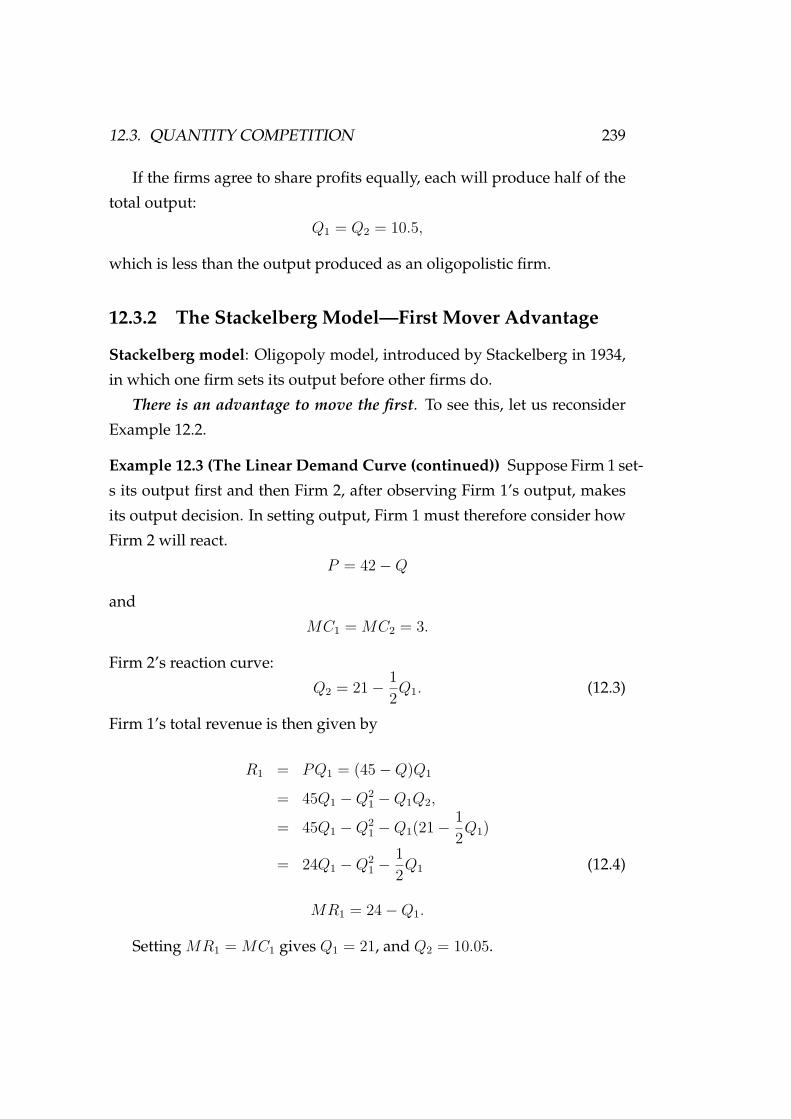
12.3. QUANTITY COMPETITION 239
If the firms agree to share profits equally, each will produce half of the
total output:
Q1 = Q2 = 10.5,
which is less than the output produced as an oligopolistic firm.
12.3.2 The Stackelberg Model—First Mover Advantage
Stackelberg model: Oligopoly model, introduced by Stackelberg in 1934,
in which one firm sets its output before other firms do.
There is an advantage to move the first. To see this, let us reconsider
Example 12.2.
Example 12.3 (The Linear Demand Curve (continued)) Suppose Firm 1 set-
s its output first and then Firm 2, after observing Firm 1’s output, makes
its output decision. In setting output, Firm 1 must therefore consider how
Firm 2 will react.
P = 42 − Q
and
MC1 = MC2 = 3.
Firm 2’s reaction curve:
Q2 = 21 − 12
Q1. (12.3)
Firm 1’s total revenue is then given by
R1 = PQ1 = (45 − Q)Q1
= 45Q1 − Q21 − Q1Q2,
= 45Q1 − Q21 − Q1(21 − 1
2Q1)
= 24Q1 − Q21 − 1
2Q1 (12.4)
MR1 = 24 − Q1.
Setting MR1 = MC1 gives Q1 = 21, and Q2 = 10.05.

240CHAPTER 12. MONOPOLISTIC COMPETITION AND OLIGOPOLY
We conclude that Firm 1 produces twice as much as Firm 2 and makes
twice as much profit. Going first gives Firm 1 an advantage.
12.4 Price Competition
12.4.1 Price Competition with Homogeneous Products—The
Bertrand Model
The Bertrand Model is about price competition with homogeneous prod-
ucts.
Bertrand model: Oligopoly model, proposed by the French economist
Joseph Bertrand in 1883, in which firms produce a homogeneous good,
each firm treats the price of its competitors as fixed, and all firms decide
simultaneously what price to charge.
This model results in the same outcome as perfect competition even
there are just two firms.
Let’s return to the duopoly example.
P = 30 − Q,
where Q = Q1 + Q2, and
MC1 = MC2 = 3.
Q1 = Q2 = 9, and in Cournot equilibrium, the market price is $12, so that
each firm makes a profit of $81.
Now suppose that these two duopolists compete by simultaneously
choosing a price instead of a quantity.
The only possible Nash equilibrium in the Bertrand model results in
both firms setting price equal to marginal cost: P1 = P2 = $3 because no
firm can obtain higher profit by unilaterally changing its pricing strategy.
The industry output is 27 units. So each firm produces 13.5 units, and both

12.4. PRICE COMPETITION 241
firms earn zero profit.
In the Cournot model, because each firm produces only 9 units, the
market price is $12. Now the market price is $3. In the Cournot model,
each firm made a profit; in the Bertrand model, the firms price at marginal
cost and make no profit.
12.4.2 Price Competition with Differentiated Products
Now suppose that each of two duopolists has fixed costs of $20 but zero
variable costs, and that they face the same demand curves:
Q1 = 12 − 2P1 + P2,
Q2 = 12 − 2P2 + P2.
Firm 1’s profit is:
Π1 = P1Q1 − 20 = P1(12 − 2P1 + P2) − 20
= 12P1 − 2P 21 + P1P2 − 20.
Similarly, we can figure out that firm 2’s profit is given by
Π2 = P2Q2 − 20 = 12P2 − 2P 22 + P1P2 − 20.
The two firms’s profit maximizing prices are
∆Π1/∆P1 = 12 − 4P1 + P2 = 0, (12.5)
∆Π2/∆P2 = 12 − 4P2 + P1 = 0. (12.6)
Solving the above two equations, we obtain the Nash equilibrium:
P1 = P2 = 4.

242CHAPTER 12. MONOPOLISTIC COMPETITION AND OLIGOPOLY
Firm 1’s reaction curve:
P1 = 3 + 14
P2.
Firm 2’s reaction curve:
P2 = 3 + 14
P1.
The intersection of these two curves gives the above Nash equilibrium.
12.5 Kinked Demand Curve Model
Each firm in an oligopolistic industry is aware that any price change it
makes will affect the sales of other firms in the industry. Thus, D and MR
curves must take into account the reactions of rivals.
Price rigidity: Characteristic of oligopolistic markets by which firms
are reluctant to change prices even if costs or demands change.
Kinked demand curve model: Oligopoly model in which each firm
faces a demand curve kinked at the currently prevailing price: at higher
prices demand is more elastic, whereas at lower prices it is less elastic.
In order to have a kinked demand curve, it is assumed that oligopolists
expect that rivals would match price cuts but not price hikes.
P
Q
P
D
P!
P"
Dr
P#
a
b
c
b
c
dd
Figure 12.9 Demand curve which takes into account the reaction of rivals

12.5. KINKED DEMAND CURVE MODEL 243
As shown in Figure 12.9, we have:
• D: firm’s demand curve when rivals do not react to price changes.
• Dr: firm’s demand curve when rivals match any price change.
Along D, as P decreases, Q increases due to:
i) substitutability of this product for similar products in other
industries; and
ii) purchases by customers who switch away from other firms
in this industry.
Along demand curve Dr, we see that as P decreases, Q increases, but
not by as much as that along demand curve D. This is because ii) above
will no longer be true:
(1) without rival reactions
• P1 decreases to P2 ⇒ a → b;
• P1 decreases to P3 ⇒ a → c.
(2) with rival reactions
• P1 decreases to P2 ⇒ a → b′ (b′ < b);
• P1 decreases to P3 ⇒ a → c′ (c′ < c);
• If P1 increases to P0, no rival will increase its price. O-
riginal firm loses customers to other firms.
We therefore arrive at a kinked demand curve, as shown in Figure
12.10. That is, at higher prices demand is very elastic, whereas at lower
prices it is inelastic.

244CHAPTER 12. MONOPOLISTIC COMPETITION AND OLIGOPOLY
P
Q
P
b
b Demand
MR
qK
MC
MC!
MC"
Figure 12.10 A kinked demand curve
To find MR here, we need to
i) identify qK ,
ii) draw MR for D until qK is reached,
iii) extend Dr to vertical axis and draw MR beginning at qK .
In the vertical segment b to b′ the profit-maximizing rule MR = MC
yields the same (p, q) for any MC (MC2 ≥ MC1 ≥ MC0). We thus come
across the so-called price rigidity. Indeed, price rigidity is a characteristic
of oligopolistic markets by which firms are reluctant to change prices even
if costs or demands change.
12.6 Prisoners’ Dilemma–Competition vs Collu-
sion:
One game-theoretical model that has implications for oligopolist behavior
is called the prisoners’ dilemma. The prisoners’ dilemma demonstrates
how rivals could act to their mutual disadvantage. Suppose that two sus-
pects, A and B, are apprehended and questioned separately about their
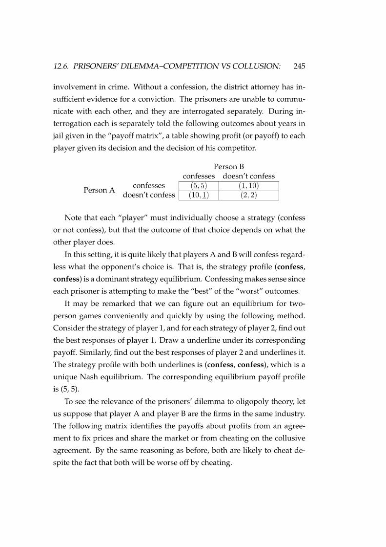
12.6. PRISONERS’ DILEMMA–COMPETITION VS COLLUSION: 245
involvement in crime. Without a confession, the district attorney has in-
sufficient evidence for a conviction. The prisoners are unable to commu-
nicate with each other, and they are interrogated separately. During in-
terrogation each is separately told the following outcomes about years in
jail given in the “payoff matrix”, a table showing profit (or payoff) to each
player given its decision and the decision of his competitor.
Person Bconfesses doesn’t confess
Person A confesses (5, 5) (1, 10)doesn’t confess (10, 1) (2, 2)
Note that each “player” must individually choose a strategy (confess
or not confess), but that the outcome of that choice depends on what the
other player does.
In this setting, it is quite likely that players A and B will confess regard-
less what the opponent’s choice is. That is, the strategy profile (confess,
confess) is a dominant strategy equilibrium. Confessing makes sense since
each prisoner is attempting to make the “best” of the “worst” outcomes.
It may be remarked that we can figure out an equilibrium for two-
person games conveniently and quickly by using the following method.
Consider the strategy of player 1, and for each strategy of player 2, find out
the best responses of player 1. Draw a underline under its corresponding
payoff. Similarly, find out the best responses of player 2 and underlines it.
The strategy profile with both underlines is (confess, confess), which is a
unique Nash equilibrium. The corresponding equilibrium payoff profile
is (5, 5).
To see the relevance of the prisoners’ dilemma to oligopoly theory, let
us suppose that player A and player B are the firms in the same industry.
The following matrix identifies the payoffs about profits from an agree-
ment to fix prices and share the market or from cheating on the collusive
agreement. By the same reasoning as before, both are likely to cheat de-
spite the fact that both will be worse off by cheating.

246CHAPTER 12. MONOPOLISTIC COMPETITION AND OLIGOPOLY
player Bcheats doesn’t cheat
player A cheats (10, 10) (20, 5)doesn’t cheat (5, 20) (15, 15)
Example 12.4 (Price Competition (continued)) Consider the same exam-
ple of duopoly: there are two firms, each of which has fixed costs of $20
and zero variable costs. They face the same demand curves:
Q1 = 12 − 2P1 + P2,
Q2 = 12 − 2P2 + P2.
We found that in Nash equilibrium each firm will charge a price of
$4 and earn a profit of $12, whereas if the firms collude, they will charge
a price of $6 and earn a profit of $16, and whereas if Firm 1 keeps the
colluding price $6 and firm 2 cheats by setting price at $4, their profits are
Π1 = P1Q1 − 20 = (6)[12 − (2)(6) + 4] − 20 = $4
Π2 = P2Q2 − 20 = (4)[12 − (2)(4) + 6] − 20 = $20,
respectively.
So if Firm 1 charges $6 and Firm 2 charges only $4, Firm 2’s profit will
increase to $20. And it will do so at the expense of Firm 1’s profit, which
will fall to $4.
Firm 2charge $4 charge $6
Firm 1 charge $4 ($12, $12) ($20, $4)charge $6 ($4, $20) ($16, $16)
Table 12.2: Payoff matrix: Table showing profit (or payoff) to each firmgiven its decision and the decision of its competitor.
Example 12.5 (Procter & Gamble in a Prisoner’s Dilemma) The Procter &

12.6. PRISONERS’ DILEMMA–COMPETITION VS COLLUSION: 247
Gamble Company (P&G) is an American multinational consumer goods
corporation headquartered in Cincinnati, Ohio, founded in 1837 by William
Procter and James Gamble. In 2014, P&G recorded $83.1 billion in sales.
It was renamed it as Procter & Gamble Health Limited in May 2019 af-
ter completing the acquisition of the consumer health division of Merck
Groupin.
Candle maker William Procter, born in England, and soap maker James
Gamble, born in Ireland, both emigrated to the US from the United King-
dom. They settled in Cincinnati, Ohio, initially and met when they mar-
ried sisters Olivia and Elizabeth Norris. Alexander Norris, their father-in-
law, persuaded them to become business partners, and in 1837 Procter &
Gamble was created.
We argued that P&G should expect its competitors to charge a price of
$1.40 and should do the same. But P&G would be better off if it and its
competitors all charged a price of $1.50.
Unilever and Kaocharge $1.40 charge $1.50
P& G charge $1.40 ($12, $12) ($29, $11)charge $1.50 ($3, $21) ($20, $20)
Table 12.3: Payoff matrix for Pricing Problem.
Since these firms are in a prisoners’ dilemma, it doesn’t matter what
Unilever and Kao do. P&G makes more money by charging $1.40.
Advertising. Another way to illustrate the usefulness of the game-
theoretical approach is to examine the interdependence of advertising de-
cisions. Suppose that two firms are considering their advertising budgets.
They have two strategies, a large budget or small budget. The payoff ma-
trix is the profits they get under different strategies. The resulting equilib-
rium strategy profile is (large budget, large budget).

248CHAPTER 12. MONOPOLISTIC COMPETITION AND OLIGOPOLY
B
Small Budget Large budget
ASmall Budget (10, 10) (5, 18)Large budget (18, 5) (8, 8)
Table 12.4: Payoff matrix for advertising game.
Unfortunately, not every game has a dominant strategy for each player
B
Small Budget Large budget
ASmall Budget (10, 8) (6, 5)Large budget (4, 2) (8, 6)
Table 12.5: Modified advertising game.
Now Firm A has no dominant strategy since its optimal decision de-
pends on what Firm B does. If Firm B chooses a small budget for advertis-
ing, Firm A does best by also choosing a small budge for advertising; but
if Firm B chooses a large budget for advertising, Firm A does best by also
choosing a large budge for advertising. Notice that although it does not
have a dominant strategy equilibrium, it has two Nash equilibria: (small
budget, small budget) and (large budget, large budget).
Furthermore, does the prisoners’ dilemma doom oligopolistic firms to
aggressive competition and low profits? Not necessarily. Although our
imaginary prisoners have only one opportunity to confess, most firms set
output and price over and over again, continually observing their com-
petitors’ behavior and adjusting their own accordingly. This allows firms
to develop reputations from which trust can arise. As a result, oligopolistic
coordination and cooperation can sometimes prevail.

12.7. DOMINANT FIRM PRICE LEADERSHIP MODEL 249
12.7 Dominant Firm Price Leadership Model
Price leadership: Pattern of pricing in which one firm regularly announces
price changes that other (smaller) firms then match.
Price leadership model is another way to resolve the uncertainty of ri-
vals’ reactions to price changes. If one firm in the industry initiates a price
change, and the rest of the firms traditionally follow the leader, there is no
uncertainty about rival behavior.
A dominant firm is a firm with a large share of total sales that sets
price to maximize profits, taking into account the supply response of many
smaller firms. Price leadership by the dominant firm occurs when the
dominant firm in the industry sets a price that maximizes its profit and
allows its smaller rivals to sell as much as they want at the price so set.
In some industries, a large firm might naturally emerge as a leader,
with the other firms deciding that they are best off just matching the lead-
er’s prices, rather than trying to undercut the leader or each other. For
example, we may consider the OPEC (Organization Petroleum Exporting
Countries) as a dominant firm, and non-OPEC ones as smaller firms.
P
Q
MR
P3
D
MCSD
qT
qD
q0
P1
P2 A
D
Figure 12.11 Equilibrium price and quantity under price leadership

250CHAPTER 12. MONOPOLISTIC COMPETITION AND OLIGOPOLY
Suppose the industry demand curve is DD. Since the other smaller
firms in the industry will follow any price change initiated by the domi-
nant firm, they become price takers, and adjust output until price equals
their marginal cost. The residual demand curve confronting the dominant
firm is obtained by subtracting the quantity the other smaller firms will
produce shown by SD from market demand, yielding P1AD. The dom-
inant firm produces qD, where MCD = MRD, and charges P3. Smaller
firms produce q0.
12.8 Cartels and Collusion
Cartel: Producers explicitly agree to cooperate in setting prices and output
levels.
In all models discussed so far, the firms were assumed to behave in-
dependently. Each firm makes a specific conjecture regarding how other
firms will respond to its action without any concern for how this affects
the profits of the other firms. That is, there is no cooperation among firms.
The most important cooperative model of oligopoly is the cartel model.
A cartel is an explicit agreement among independent producers to coor-
dinate their decisions so each of them will earn monopoly profits. If pro-
ducers adhere to the cartel’s agreements and market demand is sufficiently
inelastic, the cartel may drive prices well above competitive levels.
Cartels are often international. While U.S. antitrust laws prohibit Amer-
ican companies from colluding, those of other countries are much weaker
and are sometimes poorly enforced. Furthermore, nothing prevents coun-
tries, or companies owned or controlled by foreign governments, from
forming cartels. For example, the OPEC cartel which is formed in 1960
is an international agreement among oil-producing countries which has
succeeded in raising world oil prices above competitive levels.

12.8. CARTELS AND COLLUSION 251
Cartelization of a Competitive Industry
Dollars
per unit
Output
mr*
P
d*
q1
q2
q
P1
SMC
SAC
d
(35) (50)
Firm Dollars
per unit
Output
P
Q1
Q
P1
D
(700) (1000)
MarketSS
MR
Figure 12.12 The emergence of cartels in a competitive market
Let us see how a group of firms in a competitive market can earn monopoly
profit by coordinating their activities. We assume that the industry is ini-
tially in a long-run equilibrium, and then will identify the short-run ad-
justments (with existing plants) that the industry’s firms can make to reap
monopoly profits for themselves. Figure 12.12 shows this possibility.
Under competitive conditions, industry output is Q and price is P . If
the firms in the industry form a cartel, output is restricted to Q1 in order to
charge price P1, the monopoly outcome. Each firm produces q1 and makes
a profit at price P1.
Firms can always make a larger profit by colluding rather than by com-
peting. Acting independently, competitive firms are unable to raise price
by restricting output, but when they act jointly to limit the amount sup-
plied, price will increase. Cartel pricing can be analyzed by using the dom-
inant firm model (see Figure 12.11).
There are two conditions for cartel success:
• First, a stable cartel organization must be formed whose members

252CHAPTER 12. MONOPOLISTIC COMPETITION AND OLIGOPOLY
agree on price and output levels and then adhere to that agreement.
• The second condition, and may be the most important, is the poten-
tial for monopoly power. Even if a cartel can solve its organizational
problems, there will be little room to raise price if it faces a highly
elastic demand curve.
Why Cartels Fail?
If cartels are profitable for the members, why are not there many more?
One reason is that in the United States they are illegal. But they were rare
and were short-lived even before there were such laws. Three important
factors appear to contribute to cartel instability.
1. Each firm has strong incentive to cheat on the cartel agree-
ment as shown in prisoners’ dilemma. (Say, the above fig-
ure, if one firm enlarge its output with price P1, it can earn
much more profit.) Yet, if many firms do so, industry out-
put will increase significantly, and price will fall below the
monopoly level. It is in each firm’s interest to have other
firms restrict their output while to increase its own output.
2. Members of the cartels will disagree over appreciate cartel
policy regarding prices, output, market shares, and prof-
it sharing. This is true when cost, technology, and size of
firms are different.
3. Profit of the cartel members will encourage entry into the
industry. If the cartel achieves economic pro its by raising
the price, new firms have an incentive to enter the market.
If the cartel cannot block entry of new firms, price will be
driven back down to the competitive level as production
from the “outsiders” reaches the market.

Chapter 14
Employment and Pricing of
Inputs
The emphasis now shifts from product markets to input (or factor) mar-
kets. We will begin to look more closely at factors that determine the level
of employment and prices of inputs used to produce a product. Firms are
suppliers in product markets, and they are also demanders in input mar-
kets. Households and individuals are the demanders in product markets
while the suppliers in input markets.
In this chapter, we will discuss the basic principles common to al-
l input-market analyses, regardless of whether the input refers to labor,
capital, or raw materials.
14.1 The Input Demand of a Competitive Firm
14.1.1 Firm’s Input Demand: One Variable Input
We first introduce two concepts:
• Derived input demand: Demand for an input that depends on both
the firm’s level of output and the cost of inputs, and is derived from
profit maximization.
253

254 CHAPTER 14. EMPLOYMENT AND PRICING OF INPUTS
• Marginal revenue product (MRP) of an input: Additional value re-
sulting from the sale of output created by the use of one additional
unit of an input.
Suppose that only one input (labor) is allowed to vary and the others
are fixed. This is a short-run setting in which labor is the only variable
input. By the law of diminishing marginal returns, the labor’s marginal
product (MPL) curve slopes downward beyond some point.
How do we measure the marginal revenue product of labor (MRPL)?
It is the additional output obtained from the additional unit of this labor,
multiplied by the additional revenue from an extra unit of output. This
important result holds for any competitive factor market, whether or not
the output market is competitive.
MRPL = MR × MPL. (14.1)
However, in a competitive output market, a firm will sell all its output
at the market price P . In this case, the marginal revenue product of labor is
equal to the marginal product of labor times the price of the product, and
reduced to the so-called the marginal value product of labor (MV PL):
MV PL = P × MPL, (14.2)
Therefore, we could convert labor’s marginal product curve MPL in-
to the marginal value product curve MV PL by multiplying the marginal
product of labor by the price of the commodity produced.
In a competitive factor market in which the producer is a price taker,
when all other inputs are fixed, the competitive firm’s input demand curve
for labor is given by
w = MV PL.
The MVP curve falls because the marginal product of labor falls as
hours of work increase.

14.1. THE INPUT DEMAND OF A COMPETITIVE FIRM 255
The input demand curve for a firm with monopoly power is given by
w = MRPL.
In this case, however, the MRP curve falls because both the marginal prod-
uct of labor and marginal revenue fall.
MPL
L15 20 25
2
3
4
MVPL
$10
$20
$30
$40
MPL
and MVPL(MP
L Px).1
Figure 14.1 The input demand curve with only labor input variable, whichis given by MV PL = MPL × Px with Px = $10 for product x.
Suppose that the daily wage rate is $30 per worker. What is the optimal
employment number of workers? The firm will hire up to the point where
the marginal value product of labor is just equal to its marginal cost. That
is, the profit-maximizing firm will hire units of labor at the point where the
marginal value product of labor is equal to the wage rate. In our case, the
profit-maximizing labor-input units are L∗ = 20. Therefore, factor markets
are similar to output markets in many ways.
The factor market profit-maximizing condition w = MV PL is equiva-
lent to the output market condition that marginal revenue equals marginal
cost. Indeed, since MV PL = MPL × P , dividing both sides of equation by
the marginal product of labor, we have
w
MPL
= P.

256 CHAPTER 14. EMPLOYMENT AND PRICING OF INPUTS
Recall that we have w/MPL = MC. Then the above equation is equivalent
to the condition of profit maximization (i.e., MC = P ) in term of output.
14.1.2 Firm’s Input Demand: All Inputs Variable
In general, a change in an input price will lead the firm to alter the de-
mand of other inputs. What is the input demand curve when all inputs
are variable?
L20 25 30
W=$30
MVPL(k=12)
$
W=$20
A
B C
MVPL
(k=10)
Figure 14.2 The input demand curve with all inputs variable.
Suppose that at initial equilibrium the hourly wage rate = $30 and
L = 20. The firm is operating at point A on MV PL where K = 10. Now
suppose wage rate decreases to w = $ 20. If k keep constant (K = 10), the
firm will increase the employment of labor to L = 25. If capital increases
to K = 12 (for more workers need more “tools”), the entire MV PL curve
shifts upward. This adjustment leads to a further increase in labor to point
C. Connecting points A and C, we get the firm’s input demand curve.
14.2 The Input Demand of Competitive Industry
The total quantity of an input hired by an industry is the sum of the quan-
tities employed by the firms in the industry. To derive the industry input

14.3. THE INPUT DEMAND OF MONOPOLY 257
demand curve, we must therefore aggregate the demand curves of the
firms. However, when deriving the firm’s input demand curve, we as-
sume that the price of the product remains unchanged. This assumption
cannot be true for an industry. When all firms simultaneously increase
output, they can sell more output only at a lower price, which must be
taken into account.
L20 27 30
W=$30
d’(Px=$8)
W
A
B
C=$20
W
d(Px=$10)
L2000 2700 3000
d’(Px=$8) .
A
B
C
W
d(Px=$10)
D
Figure 14.3 The industry demand curve in a competitive industry
14.3 The Input Demand of Monopoly
A monopoly is defined as a firm that is the sole seller of some product, but
a firm that has monopoly power in its output market does not necessarily
have market power in its input markets.
Like a competitive firm, a monopoly makes decisions about input use
such that marginal cost equals marginal revenue. Suppose input is labor.
Then, for the profit-maximizing output of product x, we have
MCL = MRx.
Since MCL = wMPL
, we have
w = MPL × MRx ≡ MRPL.

258 CHAPTER 14. EMPLOYMENT AND PRICING OF INPUTS
Thus, the marginal revenue product curve MRPL is the input demand
curve of the firm. As we know, MRx of a monopoly must be lower than
the price of output x, i.e., MRx < P at each level of output and at each
level of employment of labor, so the MRPL curve lies below the MV PL
curve which is the competitive demand curve.
L
S
MRPL=MP
L MR
X
.
MVPL=MP
L P
X
.
W
W
Figure 14.4 The relationship between MRP and MVP curves undermonopoly
Note that the employment of labor, or any other input, is lower under
monopolistic condition than under competitive condition. This result is
consistent with the result we obtained previously: A monopoly produces
less output than does a competitive industry.
14.4 The Supply of Inputs
The supply side of input markets deals with the quantities of inputs avail-
able at alternative prices. Supply curve representing the price per unit that
a firm pays for a good.
Average expenditure curve (AV): Supply curve representing the price
per unit that a firm pays for a good.
Marginal expenditure curve (ME): Curve describing the additional
cost of purchasing one additional unit of a good.
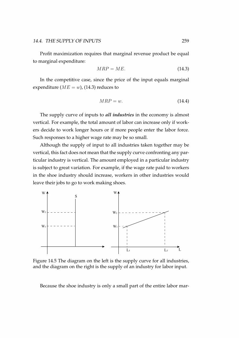
14.4. THE SUPPLY OF INPUTS 259
Profit maximization requires that marginal revenue product be equal
to marginal expenditure:
MRP = ME. (14.3)
In the competitive case, since the price of the input equals marginal
expenditure (ME = w), (14.3) reduces to
MRP = w. (14.4)
The supply curve of inputs to all industries in the economy is almost
vertical. For example, the total amount of labor can increase only if work-
ers decide to work longer hours or if more people enter the labor force.
Such responses to a higher wage rate may be so small.
Although the supply of input to all industries taken together may be
vertical, this fact does not mean that the supply curve confronting any par-
ticular industry is vertical. The amount employed in a particular industry
is subject to great variation. For example, if the wage rate paid to workers
in the shoe industry should increase, workers in other industries would
leave their jobs to go to work making shoes.
L
W!
W
W
L
W
S
W!
W
L!
Figure 14.5 The diagram on the left is the supply curve for all industries,and the diagram on the right is the supply of an industry for labor input.
Because the shoe industry is only a small part of the entire labor mar-

260 CHAPTER 14. EMPLOYMENT AND PRICING OF INPUTS
ket, its labor supply curve will be more elastic than the supply curve of
labor for the entire economy. In fact, the supply curves of most inputs
to most industries are likely to be either perfectly horizontal or slightly
upward-sloping, as shown in Figure 14.5.
14.5 Labor Supply
Since consumers are supplers of labor, we can use the consumer theory to
derive the labor supply curve.
14.5.1 The Income-Leisure Choice of a Worker
In our previous discussion of a consumer’s choice, the consumer’s income
was assumed to be fixed. However, most people’s income is not fixed but
depends instead on, among other things, the decision about how much
time the person will work. To investigate, we assume labor income is the
only source of a worker’s income, and the wage rate is fixed. Let
• I = the weekly income;
• L = the weekly leisure time;
• H = the weekly working hours;
• w = the wage rate per hour.
Then the income the consumer earns is I = wH . Since a week has
24 × 7 = 168 hours and H + L = 168, we have I = w(168 − L), and thus
I + wL = 168w,
which is the consumer’s budget constraint. The consumer’s problem is
choosing a combination of (I, L), such that he has highest utility.
Suppose the consumer’s indifference curves are strictly convex over
(I, L). We can find the optimal bundle by either graphical or mathematical

14.5. LABOR SUPPLY 261
approach. As usual, the equilibrium is the point of tangency between the
budget line and an indifference curve.
Leisure
U1
L�L�
Income
U2
U3
A
E
Leisure
Work
Figure 14.6 The income-leisure choice of a worker
14.5.2 The Supply of Working Hours
The above assumed that the wage rate was fixed. What happens if the
wage rate changes? Will workers work longer hours at a higher wage
rate? The answer depends on the consumer’s preference.
i) The substitution effect dominating the income effect implies more
working hours:
Suppose initial wage rate is w0 = $10, the optimal bundle is E. If the
wage increases to w1 = $15, the new optimal bundle is E ′. The substitution
effect = L3 − L1 < 0. The substitution effect of a higher wage rate means
to encourage a worker to have less leisure time, or to supply more hours
of labor. The income effect = L2 − L3 > 0, which means the higher wage
rate encourages the consumer to have more leisure time, or to supply less
hours of labor since income and leisure are both normal goods. The total
effect of the higher wage rate is the sum of the income and substitution
effects. Although these effects operate in opposite directions, in this case

262 CHAPTER 14. EMPLOYMENT AND PRICING OF INPUTS
the substitution effect is large, so the total effect is an increase in working
hours from NL1 to NL2.
LeisureL�L�
Income
L N
A
B
C
Figure 14.7 Consumer choice when substitution effect dominates incomeeffect
LeisureL L!
Income
L"
A
BC
Figure 14.8 Consumer choice when income effect dominates substitutioneffect
ii) The income effect dominating the substitution effect implies more
leisure time (less working hours):
When the income effect is larger than the substitution effect, the conclusion
is different from the above. The higher wage rate leads to a decrease in

14.5. LABOR SUPPLY 263
hours worked. Suppose that w further increases to w = 20. Total effect
= (L2 −L3)+(L3 −L1) = L2 −L1 > 0, which means the consumer increases
the leisure time.
14.5.3 Backward-bending Labor Supply Curve
When the wage rate increases, the hours of work supplied increase ini-
tially but can eventually decrease as individuals choose to enjoy more
leisure and to work less. The backward-bending portion of the labor sup-
ply curve arises when the income effect of the higher wage (which encour-
ages more leisure) is greater than the substitution effect (which encourages
more work). That is, for low values of w, the substitution effect dominates.
Beyond a threshold w∗, the income effect dominates.
Working hoursLL
Income
LeisureL
2
*
Income
2 3 1 H1 H3 H2
Figure 14.9 The emergency of backward-bending labor supply curve
Labor supply curve can be a vertical line.
Example 14.1 U = LαIβ ⇒ MRS = αIβL
, where α > 0, β > 0, and α+β = 1.
Determination of the consumer’s choice of I and L:
(1) By MRSLI = w1 , we have αI
βL= w and thus
I = βwL/α.

264 CHAPTER 14. EMPLOYMENT AND PRICING OF INPUTS
(2) Substituting I = βwL/α into the budget constraint I +wL =168w, we have
βwL
α+ wL = 168w
or
(β
α+ 1)wL = 168w,
and therefore
L∗ = 168α.
The consumer works 24α hours a day.
This is true for all wage rate W . That is, L∗ is independent of w.
W
LS
L*
Ld
Figure 14.10 A vertical labor supply curve
The Market Labor Supply Curve
To go from an individual’s supply curve of hours of work to the market
supply curve, we need only add (horizontally sum) the responses of al-
l workers competing in a given labor market. Thus, the market supply
curve can also slope upward, bend backward, or be a vertical line.
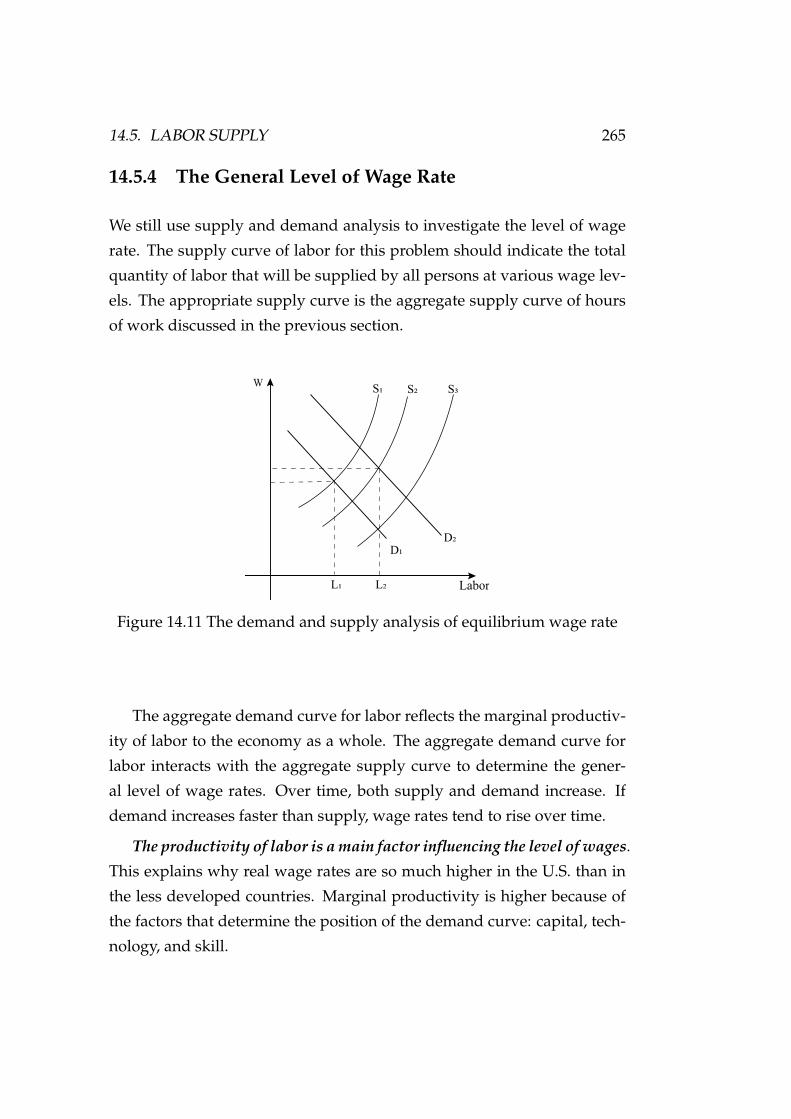
14.5. LABOR SUPPLY 265
14.5.4 The General Level of Wage Rate
We still use supply and demand analysis to investigate the level of wage
rate. The supply curve of labor for this problem should indicate the total
quantity of labor that will be supplied by all persons at various wage lev-
els. The appropriate supply curve is the aggregate supply curve of hours
of work discussed in the previous section.
Labor
W
L L!
D
D!
S S! S"
Figure 14.11 The demand and supply analysis of equilibrium wage rate
The aggregate demand curve for labor reflects the marginal productiv-
ity of labor to the economy as a whole. The aggregate demand curve for
labor interacts with the aggregate supply curve to determine the gener-
al level of wage rates. Over time, both supply and demand increase. If
demand increases faster than supply, wage rates tend to rise over time.
The productivity of labor is a main factor influencing the level of wages.
This explains why real wage rates are so much higher in the U.S. than in
the less developed countries. Marginal productivity is higher because of
the factors that determine the position of the demand curve: capital, tech-
nology, and skill.

266 CHAPTER 14. EMPLOYMENT AND PRICING OF INPUTS
14.5.5 Why Wages Differ?
We know that there is a tendency for wage rates among firms or industries
to equalize under the assumptions that workers were identical, and they
evaluated the desirability of the jobs only in terms of the monetary wage
rates. Dropping these assumptions leads to the conclusion that wage rates
can differ among jobs and among people employed in the same line of
work. Why is the wage rate for engineers higher than the wage rate for
clerks? These differences are in full equilibrium with no tendency for the
wage rates to equalize.
Labor services
of engineers
Lc
W
Labor services
of clerks
D
We
D
Le
S
S
c
Figure 14.12 Wage rate gap between engineers and clerks
There are three main factors leading to equilibrium wage differences:
a) Equalizing wage differentials: Workers currently employed
as clerks may prefer their current jobs despite the financial
difference. Monetary consideration is not the only factor,
and sometimes not the most important factor, that influ-
ences the job selections of individuals. The differences of
wages generated by preference on job choices are called e-
qualizing wage differentials because the less attractive jobs
must pay more to equalize the real advantages of employ-
ment among the jobs.

14.6. INDUSTRY DETERMINATION OF PRICE AND EMPLOYMENT OF INPUTS267
b) Differences in human capital investment: Acquiring the
skills to become an engineer may have a significant cost.
The wage for engineers may not be sufficiently high to com-
pensate clerks for the training costs they would have to bear
to become engineers.
c) Differences in ability: Even if there were no training costs,
clerks may not have the aptitude for science and mathemat-
ics necessary to work as engineers.
14.6 Industry Determination of Price and Employ-
ment of Inputs
14.6.1 The market equilibrium for labor input
D
W
L
WFirm
LL*
Industry
S
L*
Figure 14.13 The market equilibrium for labor input
As usual, the market equilibrium of an input for a particular industry will
be established when the quantity demanded equals the quantity supplied.
Graphically, the equilibrium is shown by the intersection of the industry
demand and supply curves. The position of a firm in equilibrium can be
similarly determined.

268 CHAPTER 14. EMPLOYMENT AND PRICING OF INPUTS
Note that each firm is in the position of employing the quantity of the
input at which the marginal value product equals the price.
Process of Input Price Equalization across Industries
When several industries employ the same input, the input tends to be al-
located among industries so that its price is the same in every industry. If
this were not true—if workers were receiving $40 in industry A and $30
in industry B—input owner would have incentive to shift inputs to indus-
tries where pay is higher, and this process tends to equalize input prices.
L
Industry A
L
Industry B
SA S
A
DA
$40
$30
SB
SB
DB
$30
$20
Figure 14.14 Wage rate equalization across two industries
14.6.2 Economic Rent
Rent: the payments made to lease the services of land, apartments, equip-
ment, or some other durable assets.
Economic Rent: The difference between the payments made to a factor of
production and the minimum amount that must be spent to obtain the use
of that factor.

14.6. INDUSTRY DETERMINATION OF PRICE AND EMPLOYMENT OF INPUTS269
Economic Rent with Vertical Supply Curve
The vertical curve intercuts with the demand curve for the services to de-
termine its price. The price and quantity are specified to indicate that we
are not concerned with the sale price of the land but with the price for the
services yielded by the use of land. When the supply curve of an input
is vertical, the entire remuneration of the input represents economic rent
since the same quantity would be available even at a zero price.
D
S
P
P
Q Land
Figure 14.15 Economic rent under a vertical supply curve of land
Economic Rent with an Upward-sloping Supply Curve
D
S
1 2 3 4 5 6
A�
A�
B�
B�
C�
D�
E�
C�
D�
Figure 14.16 Economic rent with an upward-sloping supply curve

270 CHAPTER 14. EMPLOYMENT AND PRICING OF INPUTS
Consider the supply of college professors. With an upward-sloping input
supply curve, part of the payment to input owners represents rent. In this
case individuals A, B, C, and D receive rents equal to areas A2, B2, C2, and
D2, respectively.
Whenever the supply curve slopes upward, part of the payments to in-
puts will be economic rents. The more inelastic the supply curve, the large
rents are as a fraction of total payments. Note that rents are the net ben-
efits received by owners of inputs from their current employment. They
measure the gains from voluntary exchange.
14.7 Factor Markets with Monopsony Power
In some factor markets, buyers have monopsony power that allows them
to affect the prices they pay. Often this happens either when one firm is a
monopsony buyer or there are only a few buyers, in which case each firm
has some monopsony power.
Firms with monopsony power buy large quantities and can negotiate
lower prices than those charged smaller purchasers.
The pure monopsony here means a single firm that is the sole purchas-
er of some type of input. It faces the market supply curve of the input, a
curve that is frequently upward sloping. An upward-sloping supply curve
for labor means that the firm must pay a higher wage rate to increase the
number of workers it employs. Thus, the marginal cost of hiring anoth-
er worker, which is ME, is not equal to the wage rate it must pay to all
workers (ME > W ), and therefore ME lies above S.
The intersection of ME and the input demand curve determines em-
ployment, i.e.,
MV PL = ME > w
if the firm is a competitor in its output market, and
MRPL = ME > w

14.7. FACTOR MARKETS WITH MONOPSONY POWER 271
if the firm is a monopoly in its output market.
Thus, in comparison with competitive input conditions, employmen-
t is lower under monopsony and so is the wage rate paid. A similarity
between monopsony and monopoly is apparently true from this conclu-
sion. A monopoly restricts output in order to set a higher price; a monop-
sony restricts output (consequently less input) in order to pay a lower
wage rate. A monopoly is able to charge a higher price because it faces
a downward-sloping demand curve; a monopsony is able to pay a lower
wage rate because it faces an upward-sloping supply curve.
Units of input
C
ME
S = AE
D=MRP = MVL
Price
(per unit
of input)
L
L*
w*=13
w!
1 2 3 4 5 6
5
10
15
20
Figure 14.17 Marginal and average expenditure
Indeed, from Figure 14.17, when the buyer of an input has monopsony
power, the marginal expenditure curve lies above the average expendi-
ture curve because the average expenditure curve is upward sloping. The
number of units of input purchased is given by L∗, at the intersection of
the marginal revenue product and marginal expenditure curves. The cor-
responding wage rate w∗ is lower than the competitive wage wc.

272 CHAPTER 14. EMPLOYMENT AND PRICING OF INPUTS
14.8 Summary of the Main Results
Summarizing the discussions in this chapter, we can express the main re-
sults in one diagram depicted in Figure 14.18:
Wage
per
worker
Number of workwers
S=AE
D=MRP L
D=MVP
L! L"
w"
w!w#w$ L
MC = ME L
L#L$
Figure 14.18 The profit-maximizing level of employment in various typesof markets
(1) When the markets for labor and product are both perfect-
ly competitive, the profit maximizing level of labor occurs
where MV PL = w. The number of units of input purchased
is given by L1, and the corresponding wage rate is w1.
(2) When the market for labor has monopsony power and the
market for product is perfectly competitive, the profit max-
imizing level of labor occurs where MV PL = ME > w. The
number of units of input purchased is L2 that is lower than
L1, and the corresponding wage rate w2 is lower than the
competitive wage w1.
(3) When the market for labor is perfectly competitive and the
market for product has monopoly power, the profit maxi-
mizing level of labor occurs where MRPL = w. The num-
ber of units of input purchased is L3 which is lower than

14.8. SUMMARY OF THE MAIN RESULTS 273
L1, and the corresponding wage rate w3 is lower than the
competitive wage w1.
(4) When the market for labor has monopsony power and the
market for product has monopoly power, the profit maxi-
mizing level of labor occurs where MV PL = ME > w. The
number of units of input purchased is given by L4 lower
than L2, and the corresponding wage rate w2 is lower than
the competitive wage w3.