Voluntary Debt Exchanges in Sovereign Debt Markets1

Juan Carlos Hatchondo Leonardo Martinez Cesar Sosa PadillaIndiana University and Richmond Fed IMF McMaster University

Preprint submitted to Elsevier October 30, 2013

1. Introduction

In sovereign debt restructurings the government swaps previously issued debt for new debt.

This paper studies restructurings that are characterized by (i) the absence of missed debt pay-

ments prior to the restructurings, (ii) reductions in the government’s debt burden, and (iii)

increases in the market value of debt claims for holders of the restructured debt. Since both

the government and its creditors are likely to benefit from such restructurings, we label these

episodes as “voluntary” debt exchanges.2

We first show evidence that some recent sovereign debt restructurings fit within our definition

of a voluntary debt exchange. We then show that a sovereign default model a la [12] can account

for voluntary exchanges. Finally, we show that within our framework, and in spite of benefiting

all parties involved at the time of the restructuring, voluntary debt exchanges are not always

optimal for the government from an ex-ante perspective.

Formally, we analyze a small open economy that receives a stochastic endowment stream of

a single tradable good. The government is benevolent, issues long-term debt in international

markets, and cannot commit to repay its debt. Sovereign debt is held by risk-neutral foreign

investors. We extend this baseline model of sovereign default by allowing for voluntary debt

exchanges. We assume that the cost of debt exchanges is stochastic and may be either low (zero)

or high. The high cost is assumed to be high enough to prevent the government from launching

a voluntary exchange. This assumption intends to capture difficulties in the implementation

of voluntary exchanges. At the beginning of each period, the debt exchange cost is realized

together with the endowment shock. When the cost is low, the government chooses whether to

conduct a voluntary debt exchange. If the government conducts a voluntary exchange, the post-

exchange debt level is endogenously determined as the outcome of a Nash bargaining game. If

the government does not conduct a voluntary exchange, it decides whether to declare an outright

2Our definition of voluntary exchange should not be interpreted as indicating that the participation of allcreditors in the exchange was strictly voluntary. First, it is difficult to determine the extent to which governmentscoerced bondholders into participating in a debt exchange (13; 37). Furthermore, even when a debt restructuringis beneficial for creditors as a group, individual creditors could benefit from free-riding on the participation ofother creditors. For a discussion of collective action problems associated with debt restructuring see [35] and thereferences therein.

2

default. An outright default is followed by a stochastic period of exclusion from capital markets

and lower income levels while this exclusion lasts.

Why does a debt relief lead to capital gains for the holders of restructured debt? In our model

this occurs because lower debt levels reduce future default risk and thus increase the market value

of the bond holders’ debt portfolio. Figure 1 shows the market value of debt as a function of the

debt stock. If the state of the economy is represented by a point like A, a marginal decline of the

debt level is more than compensated by an increase in bond prices, producing an increase in the

market value of bond holders’ debt portfolio. In this case, both the government and its creditors

could benefit from a debt restructuring that reduces the debt stock (for example, to point B).

We show that our model can account for the frequency of voluntary debt exchanges suggested

by the findings in [7], while still accounting for other features of the data highlighted in the

sovereign debt literature. Using a calibration for an archetypical emerging economy, opportunities

for voluntary debt exchanges arise in 11 percent of the simulation periods. That is, in 11 percent

of the simulation periods the initial debt level is higher than the debt level that maximizes

the market value of debt claims. We show that those periods arise after sufficiently negative

aggregate income shocks. However, an outright default does not need to be imminent in all those

periods—i.e., the government would not necessarily default if the cost of conducting a voluntary

exchange was high. The presence of voluntary exchanges in periods without an imminent default

is only possible in our model because we allow the government to issue long-term debt.

Among voluntary debt exchanges that prevented an outright default in the period of the

exchange, the average capital gain from holdings of the restructured debt is 141 percent. The

sovereign enjoys an average debt reduction of 23 percent and an average welfare gain at the times

of the exchange equivalent to permanent consumption increase of 0.6 percent. Among voluntary

debt exchanges conducted in periods in which the government would have chosen to stay current

on its debt, the average capital gain is 6 percent, the average debt reduction is 7 percent, and

the sovereign enjoys an average welfare gain equivalent to permanent consumption increase of

0.2 percent.

In spite of the Pareto gains that result at the moment of a voluntary exchange, eliminating the

possibility of conducting a voluntary exchange may improve welfare from an ex-ante perspective.

3

The anticipation of future voluntary exchanges leads lenders to offer lower prices for government

bonds. This impairs the possibility to bring future resources forward and is costly for an impatient

government that is eager to borrow. This finding highlights a cost of initiatives to facilitate

sovereign debt restructurings.

1.1. Related literature

The possibility that a sovereign debtor and its creditors can jointly benefit from a debt reduc-

tion is discussed by [14], [24], [25], and [32], among others. They present “debt overhang” models

with exogenous debt levels and show that debt relief generates Pareto gains when future debt

obligations are high enough to lower aggregate investment. By increasing aggregate investment,

a debt relief increases the resources available for creditors to confiscate in the case of a default.3

In contrast, we present a model in which a debt relief has no effect on future available resources

but it weakens incentives to default, producing capital gains for debt holders. Our findings also

complement their results by showing that (i) opportunities for Pareto improving debt reliefs arise

endogenously in a calibrated model with empirically plausible implications, and (ii) governments

may want to prevent debt reliefs from an ex-ante perspective, even when these reliefs generate

Pareto gains at the time of the debt restructuring.

[1] study a model with endogenous debt levels in which a government that cannot commit to

future actions may accumulate excessive debt claims causing a debt overhang effect on invest-

ment. The optimal allocation under no commitment lies on the constrained efficient frontier,

which rules out the possibility of mutually beneficial debt reductions once the sovereign is in a

situation of debt overhang. In contrast, we focus on debt reliefs that produce Pareto Gains at

the time of the restructuring even though they may not be optimal from an ex-ante perspective.

In the recent quantitative papers on sovereign default that followed [2] and [4], the possibility

of engaging in mutually beneficial debt relief is ruled out by assumption. We extend the baseline

model by allowing for this possibility which enables us to account for some of the heterogeneity

3It should be noted that creditors have recently faced difficulties when intending to confiscate assets of adefaulting country (see, for instance, 29 and 17). In many countries (including the U.S.), there are legal proceduresthat creditors may follow once individuals or corporations renege on their debt. Creditors rely on the enforcementof domestic courts to get—partially—repaid. However, it is difficult for courts to enforce government payments.

4

among debt restructurings. We show that the model can account for voluntary debt exchanges

while still accounting for other features of the data emphasized in the sovereign default literature.

The rest of the article proceeds as follows. Section 2 argues that some recent sovereign

debt restructurings fit within our definition of a voluntary debt exchange. Section 3 presents

a 4-period model that shows that voluntary debt exchanges arise in equilibrium and that they

can be detrimental to ex-ante welfare. Section 4 introduces the model. Section 4 discusses the

calibration. Section 6 presents the results. Section 7 concludes.

2. Voluntary debt exchanges in the data

This Section presents evidence that shows that some recent sovereign debt restructurings

fit within our definition of a voluntary debt exchange. Recall that we define a voluntary debt

exchange as a debt restructuring such that (i) the government does not miss any debt payment

prior to the restructuring, (ii) there is a decline in the government’s debt burden, and (iii) bond

holders enjoy capital gains from participating in the restructuring.

A significant fraction of sovereign debt restructurings were not preceded by missed debt

payments. For instance, [7] study 180 sovereign debt restructurings between 1970 and 2010 and

show that in 77 of these 180 restructurings the government did not miss debt payments prior to

the restructuring.

Most sovereign debt restructurings are characterized by debt reductions. Measuring the

implied debt reductions requires assumptions that allow for the comparison of debt instruments

with different characteristics. One measure of debt reduction is the “haircut”. There are different

haircut measures. Recently, the one proposed by [33] has been widely accepted and used (see for

example 7):

Haircut = 1−Present value of debt obtained in the restructuring

Present value of debt surrendered in the restructuring, (1)

where both present values are computed using the yields of the debt received at the moment of

the restructuring. Using this measure, [7] find that only 6 of the 180 restructurings they study

present negative haircuts. This indicates that governments benefited from a debt reduction in

5

the remaining 174 cases.4

We find that some recent sovereign debt restructurings that occurred in the absence of missed

debt payment were characterized by a lower debt burden for the government and a higher market

value of the debt claims of holders of restructured debt. We compute capital gains for holders of

restructured debt using bond prices to determined the value of the debt portfolio of these bond

holders, before and after the restructurings:

Capital gain =

∑J+Ii=J+1 qi(T )×Bi

(1 + r)T−t∑J

j=1 qj(T − t)× Bj

− 1, (2)

where T denotes the period for which prices of bonds obtained in the exchange are available,

T − t denotes the period for which we compute the market value of the portfolio surrendered

in the exchange, qi(t) denotes the unit price of bonds of type i in period t, and Bi denotes the

number of outstanding bonds of type i. Equation (2) refers to a case in which the debt portfolio

(B1, ..., BJ) is exchanged for the debt portfolio (BJ+1, ..., BI+J).

We are interested on the effect of debt reductions on the market value of the creditors’ debt

portfolio. Therefore, we compute the market value of the portfolio surrendered in the exchange

at different pre-restructuring dates in an attempt to control for the effect of the anticipation of

the restructuring on this market value. If the success of the exchange is perfectly anticipated, at

the time of the exchange, the value of the portfolio surrender by lenders should be equal to the

value of the portfolio they receive in the exchange.

Table 1 presents creditors’ capital gains from holding restructured debt in six recent episodes.5

The Table reports capital gains up to six months before the exchange announcement. Details on

the construction of debt portfolio values are presented in the Appendix.

4It should be noted that debt reductions are only a partial measure of the benefits accrued to sovereign debtors.Debt restructurings typically benefit debtor governments by smoothing and/or extending the maturity profile ofdebt payments.

5Secondary market bond prices make it easier to compute the market values of debt for bond debt restructuringsthan for bank debt restructurings. [7] show that out of the 180 debt restructurings that took place between 1970and 2010, 162 were bank debt restructurings and only 18 were bond debt restructurings. Out of the 18 bond debtrestructurings, 9 occurred without the government missing debt payments prior to the restructuring. These arethe recent restructurings in Belize, Dominica, Dominican Republic, Grenada, Kenya, Moldova, Pakistan, Ukraine,and Uruguay. Table 1 presents data for the five of these restructurings for which we found bond price data, plusthe 2012 Greece restructuring.

6

Belize Dom. Rep. Greece Pakistan Ukraine Uruguay

First date with all bond prices 2/21/07 5/18/05 3/9/12 n.a. 3/30/00 9/23/03

Extended deadline for participating 2/15/07 7/20/05 4/4/12 12/13/99 3/15/00 5/22/03

Original deadline for participating 1/26/07 5/11/05 3/8/12 12/13/99 3/15/00 5/15/03

Launch of the exchange 12/18/06 4/20/05 2/24/12 11/15/99 2/14/00 4/10/03

Formal exchange announcement 8/2/06 3/30/05 2/24/12 8/15/99 2/4/00 3/11/03

Informal exchange announcement (IA) 7/15/06 4/16/04 7/21/11 1/15/99 1/14/00 2/18/03

Capital gains with price of surrendered portfolio at

First date with all bond prices 0.10 0.08 0.02 n.a -0.01 0.01

Extended deadline for participating 0.11 0.11 -0.27 0.05 0.14 0.10

Original deadline for participating 0.10 0.08 0.03 0.05 0.14 0.12

Launch of the exchange 0.05 0.04 -0.01 0.04 0.18 0.30

Formal exchange announcement -0.05 0.06 -0.01 0.00 0.24 0.28

Informal exchange announcement -0.11 0.24 -0.59 0.07 0.48 0.22

One month before IA -0.14 0.27 -0.60 0.22 0.49 0.04

Three months before IA -0.19 0.10 -0.66 -0.02 0.39 0.34

Six months before IA 0.05 n.a. -0.69 -0.38 -0.12 0.38

Acceptance rate 0.98 0.94 0.97 0.99 0.99 0.95

Haircut 0.24 0.05 64.8 0.15 0.18 0.10

Table 1: Capital gains from holdings of restructured debt in recent sovereign debt restructurings.

7

Figure 2 presents the market value of debt portfolios for the six exchanges in Table 1. Figure

2 and Table 1 show that four of the debt exchanges under consideration produced capital gains

when we considered the price of surrendered bonds at the moment of the informal announcement.

These are the episodes in Dominican Republic, Pakistan, Ukraine, and Uruguay. Figure 2 shows a

common pattern in the value of the portfolio surrendered in the exchange for these four episodes:

this value increases in the weeks preceding the exchange.

All episodes in Table 1 are characterized by debt reductions, as measured by positive haircuts

(the Table presents the haircuts computed by 7 and 37). The restructurings in Belize and Greece

had the highest haircuts among the six episodes we consider. This is consistent with the capital

losses we measure for those episodes.

Notice that the capital gain measured as in equation (2) equals the opposite of the haircut

measure (1) for the case in which present values are computed using the yield implicit in each

bond price—and thus the present value of payments promised in a bond is given by its price.

Thus, the key difference between the haircut and capital gain measures presented in Table 1 is

in the yield used to compute the present value of debt surrendered in the restructuring: for the

haircut measure we use the yields implicit in the price of bonds obtained in the restructuring,

and for the capital gain measure we use the yields implicit in the price of bonds surrendered in

the restructuring. This indicates that for the four restructurings that present capital gains—and

therefore fit within our definition of voluntary exchanges—the implied yields in sovereign bond

prices decreased after these restructurings. This could be due to a decline in country risk implied

by each restructuring, which is consistent with our theory of voluntary debt exchanges.

3. A four-period example

This Section presents a four-period model that allows us to illustrate how voluntary debt

exchanges can occur in equilibrium, and how eliminating the possibility of voluntary exchanges

may improve welfare from an ex-ante perspective. This model presents several stark assumptions

that we relax when we study the quantitative model presented in Section 4.

8

3.1. Environment

The economy lasts for four periods, denoted by t ∈ {1, 2, 3, 4}. The government receives a

sequence of endowments yt. The endowment in periods 1 and 2 is equal to y. The endowment

realization in period 3 (y3) is drawn from an uniform distribution with support [0, 1]. The

endowment realization in period 4 is drawn from an uniform distribution with support [0, y3].

In the first three periods, the government can issue sovereign bonds promising to pay one

unit of the good in period 4. That is, the maturity of bonds issued in periods 1 and 2 is higher

than one period. Foreign competitive lenders are risk neutral and face an opportunity cost of

funds equal to the real interest rate, which is assumed to be equal to zero. Each period, the

government maximizes the expected utility of a risk-neutral representative agent, who discounts

future payoffs with the factor β < 1.

In period 3, the government can conduct a voluntary debt exchange. If a voluntary exchange is

conducted, the post-exchange debt is such that it maximizes the market value of debt claims. The

cost of conducting a debt exchange for the government is zero with probability π or prohibitively

large with probability 1− π.

In period 4, the government can declare an outright default on its debt. If the government

defaults, it loses a fraction φ of its period-4 income. Thus, consumption is given by:

c1 = y + b2q1(b2),

c2 = y + (b3 − b2)q2(b3),

c3 = y3 + e[b4 − bE(b3, y3)]q3(b4, y3) + (1− e)(b4 − b3),

c4 = y4 − d(b4, y4)φy4 − [1− d(b4, y4)]b4,

where bt ≥ 0 denotes the number of sovereign bonds at the beginning of period t, qt denotes the

bond price in period t, e is an indicator function that equals 1 (0) if the cost of an exchange is

low (high), bE denote the government debt level after the exchange stage when the cost of an

exchange is low, and d denotes government’s outright default decision that takes a value of 1 (0)

when the government chooses to default (repay).

9

3.2. Results

We solve the model backwards. Next, we describe the equilibrium functions for each period.

3.2.1. Period 4

The government maximizes period-4 consumption by defaulting if and only if b4 > φy4. Thus,

d(b4, y4) =

⎧

⎨

⎩

0 if b4 ≤ φy4

1 otherwise.

3.2.2. Period 3

The period-4 default decision implies that the equilibrium bond price in period 3 is given by

q3 (b4, y3) =

⎧

⎨

⎩

1− b4φy3

if b4 ≤ φy3

0 otherwise.

Using this bond-price function, we can find the equilibrium period-3 borrowing rule. Note that

the government is indifferent among all levels of bond issuance such that b4 ≥ φy3—because for

such issuance levels q3 (b4, y3) = 0 and d(b4, y4) = 1. Let b denote the government’s debt level at

the time it chooses its period-3 borrowing (i.e., after the debt exchange stage). If b ≥ φy3, the

equilibrium b4 ≥ b is undetermined—q3 (b4, y3) = 0 and d(b4, y4) = 1 for all b4 ≥ b. We assume

that if b4 ≥ b, the equilibrium b4 = b.

At the time the government chooses its period-3 borrowing (i.e., after the debt exchange

stage), for any debt level b, the period-3 equilibrium borrowing rule is given by

b4(b, y3) =

⎧

⎨

⎩

b+(1−β)φy32−β

if b ≤ φy3

b otherwise.

Thus, the debt market value after the debt exchange stage is equal to

MV3(b, y3) = bq3(

b4(b, y3), y3)

=

⎧

⎨

⎩

φyb−b2

φy(2−β) if b ≤ φy3

0 otherwise.

10

The debt level that maximizes this market value is φy3/2. Therefore, a debt exchange would

only be conducted if b3 > φy3/2 (and thus the government benefits from a debt reduction).

Consequently,

bE(b3, y3) = min{b3,φy3/2}.

The analysis above implies that as long as it is possible that a voluntary debt exchange is not

too expensive (π > 0), and the government chooses to start period 3 with a positive debt level

(b3 > 0), voluntary debt exchanges are part of the equilibrium of this model. In particular, the

probability of observing a voluntary debt exchange is given by max{

2π b3φ, 1}

.

3.2.3. Period 2

The following proposition characterizes the period-2 bond price function (proofs are presented

in the Appendix):

Proposition 1 (Period-2 bond price function). The equilibrium period-2 bond price func-tion q2 is increasing with respect to the probability of a voluntary exchange π. If π = 0, q2 (b3) = 0for all b3 ≥ φ. In contrast, if π > 0, q2 (b3) > 0 for all b3 ≥ 0. Furthermore, lim

b3→∞q2(b3) = 0.

Proposition 1 shows that the possibility of a voluntary debt exchange lowers the period-2 financial

cost of borrowing. That is because the expected debt recovery will be increased in period 3 if the

government starts with a sufficiently large debt stock. We show next that, in contrast to what

is observed in period 2, the borrowing cost may increase in period-1. In order to do so, we focus

on the extreme case in which is always free for the government to conduct a voluntary exchange

in period 3 (π = 1; when we study the quantitative model we calibrate π to obtain a plausible

frequency of voluntary debt exchanges). The next proposition states that for sufficiently large

debt levels contracted in period 1, the government fully dilutes those claims in period 2.

Proposition 2 (Full debt dilution). Suppose π = 1. There is a threshold b ≤ φ/2 such that,b3(b2) = +∞ for any b2 ≥ b.

In order to provide intuition for proposition 2, consider the case in which the government

enters period 2 with a debt level that, in the absence of new issuances, implies a probability 1 of

11

being renegotiated and reduced down to φy3/2 in period 3. In that case, the best strategy for a

government that prefers to bring consumption forward (β < 1) is to assign de facto seniority to

bond holders who buy debt issued in period 2. The government does so by issuing an infinitely

large amount of debt in period 2. This ensues that the share of post-exchange bonds received by

investors who purchased debt in period 1 is infinitesimal. With this strategy, the government is

able to bring consumption forward to period 2 at the expense of diluting the claims of existing

bond holders.

3.2.4. Period 1

The possibility of full dilution limits the amount of debt that the government can issue in

period 1. In addition, we show that in the cases in which the government does not fully dilute

the debt in period 2, it exploits the better borrowing terms by issuing more debt in that period,

which depresses the bond price faced by the government in period 1 (there is partial dilution).

We do so by presenting a numerical example in which a voluntary debt exchanges can occur in

equilibrium. In this example, eliminating the possibility of voluntary exchanges would improve

the period-1 expected lifetime utility. This example assumes that β = 0.75, φ = 0.5, and y = 0.

We illustrate the gains from eliminating the possibility of voluntary debt exchanges by comparing

the model economies with π = 0 and π = 1.

The left panel of Figure 3 shows that the possibility of a voluntary debt exchange (π = 1)

increases the period-1 financial cost of borrowing. In particular, with π = 1, there is a threshold

b = 0.02 such that for all b2 ≥ b, the price lenders are willing to pay for sovereign bonds is

zero. The threshold b is the one presented in Proposition 2. For all b2 ≥ b, lenders expect that

the government will choose to fully dilute the value of debt issued in period 1. Furthermore,

the price faced by the government is also lower for issuance levels below b. The reason is that

the government exploits the better borrowing terms faced in period 2 in the economy with debt

exchanges (see proposition 1) by increasing its borrowing. That is, when the government enters

period 2 with debt levels below b, it only partially dilutes those debt claims, reducing the bond

prices faced the government deciding in period 1.

The right panel of Figure 3 shows that the government is better off when it cannot conduct

12

voluntary debt exchanges (π = 0). This is the case because the possibility of conducting voluntary

debt exchanges worsens the government’s borrowing opportunities and impairs the government’s

ability to bring consumption forward. In this numerical example, the government enters period

3 with b3 > 0. This implies that voluntary debt exchanges are a feature of the equilibrium. They

are observed for period 3 income realizations y3 ∈ [0, 2b3/φ).

Summing up, we have presented a numerical example in which voluntary debt exchanges

occur in equilibrium. At the time of the debt exchange, these exchanges produce Pareto gains

by reducing the government’s debt burden while increasing the market value of debt claims.

Nevertheless, eliminating the possibility of conducting voluntary exchanges would enable the

government to achieve a more front-loaded consumption profile and increase its welfare. In this

environment, the marginal value of consumption for the government is constant. This implies

that voluntary debt exchanges do not have any insurance properties. In what follows, we study

an infinite-horizon economy in which domestic residents are risk averse. This introduces an

insurance role for voluntary debt exchanges. We find that for empirically plausible parameter

values, ex-ante welfare is reduced by the possibility of conducting voluntary debt exchanges.

4. Model

There is a single tradable good. The economy receives a stochastic endowment stream of this

good yt, where

log(yt) = (1− ρ)µ+ ρ log(yt−1) + εt,

with |ρ| < 1, and εt ∼ N (0, σ2ϵ ).

The government’s objective is to maximize the present expected discounted value of future

utility flows of the representative agent in the economy, namely

Et

∞∑

j=t

βj−tu (cj) ,

where E denotes the expectation operator, β denotes the subjective discount factor, and the

utility function is assumed to display a constant coefficient of relative risk aversion denoted by

γ. That is,

13

u (c) =c(1−γ) − 1

1− γ.

As in [15], we assume that a bond issued in period t consists of a perpetuity with geometrically

declining coupon obligations. In particular, a bond issued in period t promises to pay one unit

of the good in period t+ 1 and (1− δ)s−1 units in period t+ s, with s ≥ 2.

The government cannot commit to repay its debt. We refer to events in which the government

reneges on its debt as outright defaults. As in previous studies, the cost of an outright default

does not depend on the size of the default. Thus, when the government defaults, it does so on

all current and future debt obligations.6 Following previous studies, we also assume that the

recovery rate for outright defaults is zero.

An outright default triggers exclusion from credit markets for a stochastic number of periods.

Income is given by y − φ (y) in every period in which the government is excluded from credit

markets. As in [4], we assume that it is proportionally more costly to default in good times. This

is a property of the endogenous default cost derived by [27]. As in [6], we assume a quadratic

loss function for income during a default episode φ (y) = max {d0y + d1y2, 0}. They show that

this function allows the equilibrium default model to match the behavior of the spread in the

data.

Lenders are risk neutral and discount future payoffs at the rate r. Bonds are priced in a

competitive market inhabited by a large number of identical lenders, which implies that bond

prices are pinned down by a zero expected profit condition.

Our departure from the baseline setup is to allow for voluntary debt exchanges. We present

a stylized model of voluntary exchanges. We intend to capture the difficulties in implementing a

voluntary restructuring by assuming that the cost of debt exchanges is i.i.d. and may take a low

(zero) or a high value. The high cost is assumed to be sufficiently elevated to make it optimal

for the government to not launch a voluntary exchange when the cost is high.7

6This is consistent with the behavior of defaulting governments in reality. Sovereign debt contracts often con-tain acceleration and cross-default clauses. These clauses imply that after a default event, future debt obligationsbecome current (see 21).

7Voluntary exchanges may be prevented because of collective action problems (35), which are sometimes

14

When the cost of a voluntary exchange is zero, the government chooses whether to conduct

an exchange. If the government conducts a voluntary exchange, it reduces its debt level. We

assume that the post-exchange debt level is endogenously determined in a Nash bargaining game

in which the government and bond holders negotiate over the debt level.8

The government cannot commit to future outright default, exchange, and borrowing deci-

sions. Thus, one may interpret this environment as a game in which the government making the

exchange, default, and borrowing decisions in period t is a player who takes as given the exchange,

default and borrowing strategies of other players (governments) who will decide after t. We focus

on Markov Perfect Equilibrium. That is, we assume that in each period, the government’s equi-

librium exchange, default and borrowing strategies depend only on payoff-relevant state variables.

[26] discuss the possibility of multiple Markov perfect equilibria in infinite-horizon economies.

In order to avoid this problem, we solve for the equilibrium of the finite-horizon version of our

economy. That is, we increase the number of periods of the finite-horizon economy until value

functions and bond prices for the first and second periods of this economy are sufficiently close.

We then use the first-period equilibrium policy functions as an approximation of the stationary

equilibrium policy functions.

4.1. Recursive formulation

Let b denote the number of outstanding coupon claims at the beginning of the current period.

Let θ ∈ {L,H} denote the exchange-cost shock, where L (H) denotes the low (high) value of the

shock. Let V denote the value function of a government that is not currently in default. This

function satisfies the following functional equations:

V (b, y, L) = max{

V E(b, y), V P (b, y), V D(y)}

, (3)

mitigated by the inclusion of collective action clauses, minimum participation thresholds, and exit consents indebt contracts (see 23). We interpret a low exchange cost shock as representing circumstances in which collectiveaction problems can be overcome. We calibrate the probability of such shock targeting the frequency of voluntaryexchanges. Since voluntary exchanges in our model are only conducted when there is no cost for the sovereign,our results may provide an upper bound of the benefits derived from debt exchanges.

8We rule out the possibility that bond holders can extract side payments from the government in order toaccept a restructuring proposal.

15

and

V (b, y,H) = max{

V P (b, y), V D(y)}

, (4)

where V E denotes the continuation value when the government launches a debt exchange, V P

denotes the continuation value when the government pays its debt obligations (and does not

launch an exchange), and V D denotes the continuation value when the government declares an

outright default.

The value function of paying current debt obligations and not launching an exchange is

represented by the following functional equation:

V P (b, y) = maxb′≥0,c

{

u (c) + βE(y′,θ′)|yV (b′, y′, θ′)}

, (5)

subject to

c = y − b+ q(b′, y) [b′ − (1− δ)b] ,

where b′ − (1 − δ)b represents current debt issuances, and q denotes the price of a bond at the

end of a period. Let bP denote the government’s borrowing rule when it stays current on its debt

obligations.

The value function when the government declares an outright default satisfies the following

functional equation:

V D(y) = u (y − φ(y)) + βE(y′,θ′)|y

[

(1− ψ)V D(y′) + ψV (0, y′, θ′)]

, (6)

where ψ denotes the probability of regaining access to capital markets. Let d denote the gov-

ernment’s default strategy. The function d takes a value of 1 when the government declares an

outright default and takes a value of 0 when it stays current on its debt.

Finally, the value function when the government launches a debt exchange satisfies:

V E(b, y) = V P (bE(b, y), y), (7)

where bE(b, y) denotes the post-exchange debt level. That is, in a restructuring period the

government services the debt agreed on the restructuring and then it issues (or buys back) debt.

The post-exchange debt level is endogenously determined in a Nash bargaining game in which

bond holders’ bargaining power is constant over time and denoted by α, namely:

16

bE(b, y) = argmaxbE

{

[

MV (bE , y)−MV (b, y)]α [

V P (bE , y)−Max{

V P (b, y), V D(b, y)}]1−α

}

s.t. MV (bE , y)−MV (b, y) ≥ 0, and

V P (bE , y)−Max{

V P (b, y), V D(b, y)}

≥ 0,

where MV (b, y) denotes the market value of debt claims outstanding at the beginning of the

period. If it is optimal for the government to default when it starts with a state vector (b, y),

the market value is zero. If it is optimal to repay, the market value equals the sum of current

coupon payments and the value at which bond holders can sell their bond portfolio. Formally,

MV (b, y) = b[

1− d(b, y)] [

1 + (1− δ) q(

bP (b, y), y)]

. (8)

The surplus that each party obtains in the restructuring consists of the difference between

the continuation value if the restructuring takes place and the continuation value without re-

structuring. If a restructuring does not take place, the market value of bond holders’ debt claims

is MV (b, y) and the continuation value for the government is Max{

V P (b, y), V D(b, y)}

. If a

restructuring that brings the debt level to bE takes place, the market value of bond holders’ debt

claims is MV (bE , y) and the continuation value for the government is V P (bE , y).

Let e denote government’s exchange strategy. The function e takes a value of 1 when the

government chooses to conduct a debt exchange. Recall we assume that the high cost of an

exchange is such that e(b, y,H) = 0 for all (b, y).

The assumption that bond holders price bonds in competitive markets implies that

q(b′, y)(1 + r) = E(y′,θ′)|y

{

e (b′, y′, θ′)bE(b, y)

b′

[

1 + (1− δ) q(bP (bE(b′, y′), y′), y′)]

+ [1− e (b′, y′, θ′)][

1− d (b′, y′, θ′)] [

1 + (1− δ) q(bP (b′, y′), y′)]}

, (9)

where bE(b,y)b′

≤ 1 denotes the number of bonds received in the exchange per bond surrendered.

Notice that the model equivalent of the definition of haircut presented in the introduction is

given by 1− bE(b,y)b′

.

17

4.2. Equilibrium definition

A Markov Perfect Equilibrium is characterized by

1. rules for voluntary exchanges e, default d, and borrowing bP ,

2. and a bond price function q,

such that:

i. given a bond price function q, the policy functions d, e, and bP solve the Bellman equations

(3), (4), (5), (6), and (7).

ii. given policy rules d, e, and bP , the bond price function q satisfies condition (9).

5. Calibration

Table 2 presents the benchmark values given to the parameters in the model. A period in

the model refers to a quarter. The coefficient of relative risk aversion is set equal to 2, the

risk-free interest rate is set equal to 1 percent, and the discount factor is set equal to 0.975.

These are standard values in quantitative business cycle and sovereign default studies. The

average duration of sovereign default events is three years (ψd = 0.083), in line with the duration

estimated by [10].

We use Mexico as reference for the calibration. Mexico is an archetypical emerging economy

that is commonly used as reference in previous work that studies these economies (see, for

example, 3, 28, and 34). The parameter values that govern the income process are estimated

using GDP data from the first quarter of 1980 to the fourth quarter of 2011.

We set δ = 3.3 percent. With this value, bonds have an average duration of 5 years in the

simulations, which is roughly the average debt duration observed in Mexico according to [8].9

We allow creditors to have full bargaining power during the debt exchange bargaining game.

In terms of Figure 1, this means that if the government conducts a debt exchange in a period

9We use the Maculae definition of duration that, with the coupon structure in this paper, is given by D = 1+r∗

δ+r∗,

where r∗ denotes the constant per-period yield delivered by the bond. Using a sample of 27 emerging economies,[8] find an average duration of foreign sovereign debt in emerging economies—in 2000—of 4.77 years, with astandard deviation of 1.52.

18

Risk aversion γ 2

Risk-free rate r 0.01

Discount factor β 0.975

Probability of reentry after default ψ 0.083

Probability of high exchange shock π 0.02

Income autocorrelation coefficient ρ 0.94

Standard deviation of innovations σϵ 1.5%

Mean log income µ (-1/2)σ2ϵ

Debt duration δ 0.033

Income cost of defaulting d0 -1.01683

Income cost of defaulting d1 1.18961

Creditors bargaining power α 1

Table 2: Benchmark parameter values.

characterized by point A, it lowers its debt level to the one depicted by point B. It is often argued

that friendly restructurings maximize creditors’ recovery rate subject to bringing the debt to a

“sustainable” level. This seems consistent with our baseline of α = 1. In Subsection 6.6 we

present comparative statics with respect to α.

We calibrate the values of d0, d1, and π (the probability of a high exchange cost) targeting

the average levels of spread and debt between 1995 (due to data availability) and 2011, and a

share of voluntary debt exchanges to default episodes of 30 percent. Debt restructurings that fit

within our definition of voluntary exchange are likely to be considered sovereign defaults. For

instance, this is often the case for the four restructurings described in Section 2 (for example,

7 describe these episodes as defaults). Credit-rating agencies consider a “technical” default

an episode in which the sovereign makes a restructuring offer that contains terms less favorable

than the original debt, leaving considerable ambiguity on how to determine whether terms offered

to investors were less favorable. Usually, the haircut definition presented in Section 2 is used

19

as a measure of investor losses.10 This interpretation of the haircut would be consistent with

considering all voluntary exchanges as sovereign defaults, as we do for interpreting simulation

results. [7] report that 43 percent of the default episodes they study occur before the government

defaults on debt payments. As we show in Section 2, not all these episodes result in capital gains

for investors. Thus, 43 percent is an upper bound for the share of voluntary debt exchanges to

default episodes.

6. Results

We first show that the model simulations reproduce features of the data. We then discuss

the opportunities for voluntary debt exchanges in the simulations and the role of long-term debt

in generating these opportunities, the gains at the moment of a voluntary exchange, and the

ex-ante gains from avoiding voluntary debt exchanges. Finally, we present comparative statics

with respect to creditors’ bargaining power in determining the post-exchange debt level.

The recursive problem is solved using value function iteration. The approximated value and

bond price functions correspond to the ones in the first period of a finite-horizon economy with

a number of periods large enough to make the maximum deviation between the value and bond

price functions in the first and second period small enough. We solve for the optimal debt level

in each state by searching over a grid of debt levels and then using the best point on that grid as

an initial guess in a nonlinear optimization routine. The value functions V E, V P , and V D, and

the bond price function q are approximated using linear interpolation over y and cubic spline

interpolation over debt levels.11 We use 50 grid points for both debt and income. Expectations

are calculated using 75 quadrature points for the income shock.

In order to compute the sovereign spread implicit in a bond price, we first compute the yield

i an investor would earn if it holds the bond to maturity (forever in the case of our bonds) and

10In fact, the objective of [33] when they introduce this definition is to measure investors’ losses.11[19] discuss the advantages of using interpolation and solving for the equilibrium of a finite-horizon economy.

20

no default is ever declared. This yield satisfies

qt =1

(1 + i)+

∞∑

j=1

(1− δ)j

(1 + i)j+1.

The sovereign spread is the difference between the yield i and the risk-free rate r. We report the

annualized spread

rst =

(

1 + i

1 + r

)4

− 1.

Debt levels in the simulations are calculated as the present value of future payment obligations

discounted at the risk-free rate, i.e., bt(1 + r)(δ + r)−1, where δ = 1 for one-period bonds. We

report debt levels as a percentage of annualized income.

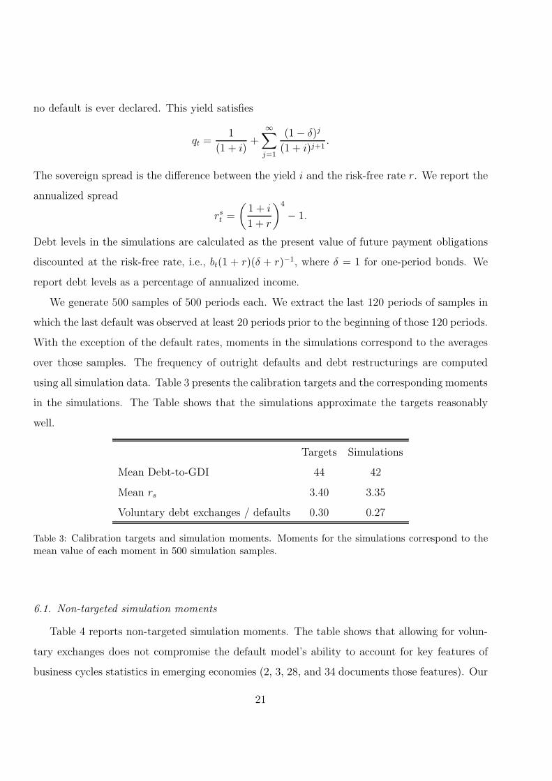
We generate 500 samples of 500 periods each. We extract the last 120 periods of samples in

which the last default was observed at least 20 periods prior to the beginning of those 120 periods.

With the exception of the default rates, moments in the simulations correspond to the averages

over those samples. The frequency of outright defaults and debt restructurings are computed

using all simulation data. Table 3 presents the calibration targets and the corresponding moments

in the simulations. The Table shows that the simulations approximate the targets reasonably

well.

Targets Simulations

Mean Debt-to-GDI 44 42

Mean rs 3.40 3.35

Voluntary debt exchanges / defaults 0.30 0.27

Table 3: Calibration targets and simulation moments. Moments for the simulations correspond to themean value of each moment in 500 simulation samples.

6.1. Non-targeted simulation moments

Table 4 reports non-targeted simulation moments. The table shows that allowing for volun-

tary exchanges does not compromise the default model’s ability to account for key features of

business cycles statistics in emerging economies (2, 3, 28, and 34 documents those features). Our

21

model is able to account for a volatile and countercyclical spread that leads to more borrowing

in good times than in bad times, as reflected by a volatile and countercyclical trade balance.

Mexico Simulations

σ (rs) 1.6 1.4

corr (rs, y) -0.5 -0.7

σ(c)/σ(y) 1.3 1.3

ρ(tb, y) -0.7 -0.8

ρ(rs, tb) 0.8 0.9

Table 4: Non-targeted simulation moments. The standard deviation of x is denoted by σ (x). The coef-ficient of correlation between x and z is denoted by corr (x, z). Moments for the simulations correspondto the mean value of each moment in simulation samples.

6.2. Voluntary debt exchanges

Opportunities for voluntary debt exchanges arise on average in 11 out of 100 simulation

periods. That is, in 11 percent of the simulation periods the initial debt level b is higher than

the debt level that maximizes the market value of debt (denoted by b(y)). There are two reasons

why this may happen. First, b may be higher than b(y) because of a sufficiently negative income

shock. Even when the government chooses bP (b, y) < b(y), it may still be that next period

bP (b, y) > b(y′). The left panel of Figure 5 depicts the market value of debt claims for two

income levels. The Figure shows that declines in income shift the market value curve towards

the origin and reduce the debt level that maximizes MV . This occurs because, as is standard

in models of sovereign default that generate countercyclical spreads, lower income levels imply

higher default probabilities. This is illustrated in the right panel of Figure 5.

Furthermore, even when the government starts the period with b < b(y), it may choose to end

a period with a debt level higher than the one that maximizes the debt market value. Figure 6

presents an example of these situations in the simulations. We find however that such examples

are only observed in 3 percent of the simulation periods. Furthermore, as illustrated in Figure

6, b′ is typically very close to b in these periods.

22

Figure 7 presents the equilibrium outright default and voluntary exchange policies. Figure

7 shows that the government prefers to participate in a debt exchange only when aggregate

income takes a sufficiently low value (grey and black areas). The income threshold at which

the government is indifferent between participating and not participating in a debt exchange

is higher than the income threshold at which it is indifferent between an outright default and

repaying current debt obligations. This also means that all outright defaults in the simulations

would have been avoided with a low cost of voluntary exchange. In addition, Figure 7 shows

that for some state realizations the government would choose to conduct a voluntary exchange

even if the impossibility of an exchange would not have triggered an outright default (grey area).

This is consistent with the presence of opportunities for capital gains at debt levels that would

not trigger an outright default, as illustrated in the left panel of Figure 5.

6.3. The role of long-term debt

Table 5 presents the benchmark simulations (when the government issues only long-term

debt) and simulations of the model with only one-period debt (δ = 1) and maintaining the

remaining parameter values presented in Table 2. When the government only issues one-period

debt, the spread and default rates are significantly lower than in the baseline calibration (see 15).

In addition, the share of default episodes that can be described as voluntary debt exchanges drop

from 27 percent in our benchmark to 2 percent with one-period debt. This is the case because in

the one-period-bond version of the model, all voluntary exchanges prevent an outright default.

Notice that with one-period bonds, the market value of the debt stock at the beginning of a

period is given by MV (b, y) =[

1− d(b, y)]

b. Therefore, a debt reduction can only increase

this market value (making a voluntary exchange possible) when the debt reduction prevents an

outright default. As illustrated in Figures 5 and 7, this is not the case with long-term debt:

at the beginning of a period, the debt level may be higher than the one that maximizes the

debt market value (generating the possibility of a voluntary exchange) even if the initial debt

level would not lead the government to default in the current period. In fact, only 5 percent of

voluntary exchanges in our benchmark simulations prevent an outright default in the period of

the exchange.

23

Benchmark One-period bonds

Mean Debt-to-GDP 42.4 32.3

Mean rs 3.35 0.14

Outright defaults per 100 years 2.21 0.14

Voluntary debt exchanges per 100 years 0.81 0.003

Table 5: Simulations in benchmark model and with one-period debt.

Furthermore, the government would never choose a debt level higher than the one that max-

imizes the debt market value in the one-period-bond version of the model. Such a choice is

only optimal when the issuance proceeds are different from the market value (as in our baseline

calibration with long-term debt). This is not the case with one-period bonds.12 Choosing a debt

level higher than the one that maximizes the debt market value implies choosing a debt level

such that the effect of additional borrowing on the market value is negative. If the government

repays its debt and does not launch a voluntary exchange, the first order condition for debt

accumulation is given by:

d (q (b′, y) b′)

db′= −

β

u′(c)

d(

E(y′,θ′)|yV (b′, y′, θ′))

db′+ (1− δ) b

d (q (b′, y′))

db′, (10)

assuming the value and bond price functions are differentiable.

The left hand side of equation (10) represents the marginal effect of the last bond issued in

the period on the market value of debt claims outstanding at the end of the period. In the model

simulations, the first term of the right hand side is always positive (the government is worse off

when it starts a period with a higher debt level) while the second term is negative (bond prices

are lower when the government chooses a higher debt level). Thus, the government only chooses

debt levels higher than the one that maximizes the market value when that second term is low

enough. This is never the case in the one-period-bond version of the model (δ = 1), where the

second term is equal to zero.

12When the government issues debt, it is concerned about the market value of the debt claims that it is issuing(i.e., the issuance proceeds) and not about the overall value of the debt stock (see 20). With one-period debt,debt issued in the current period constitutes the total debt stock.

24

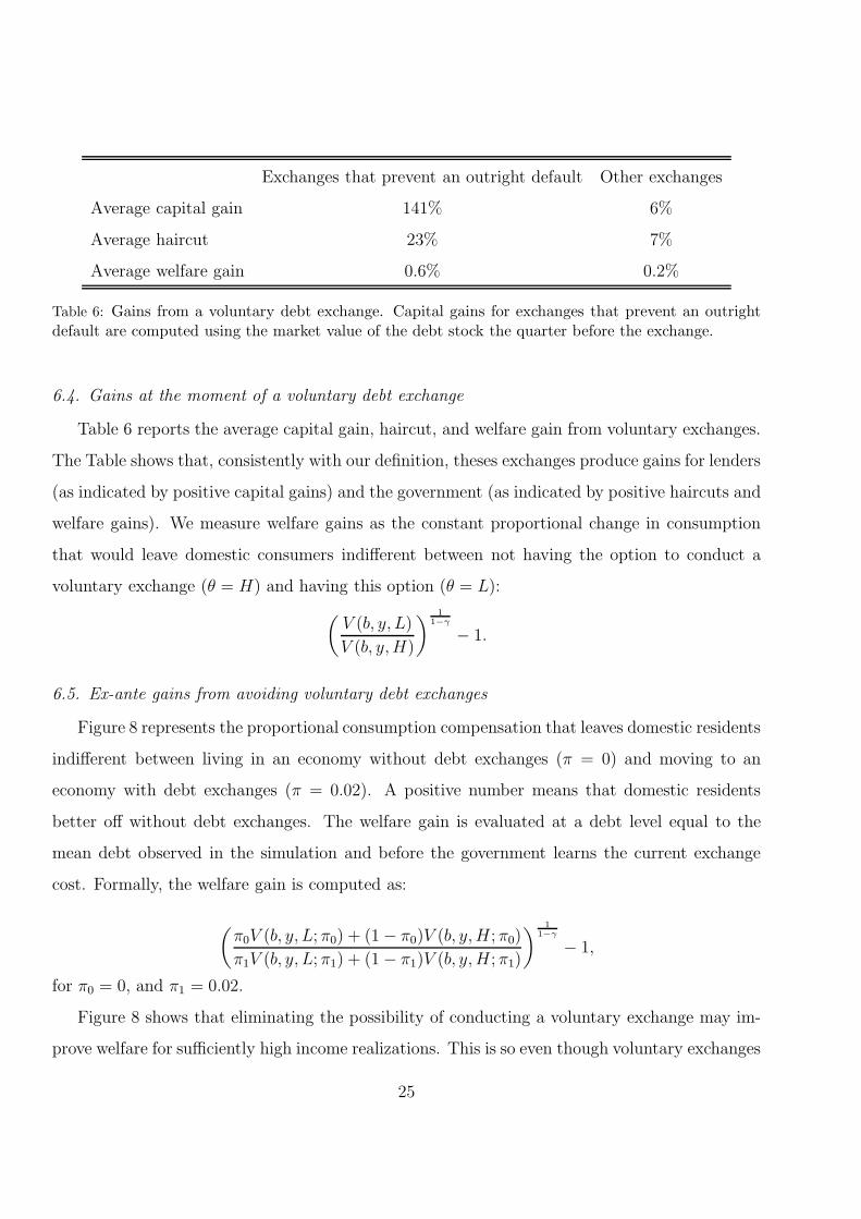
Exchanges that prevent an outright default Other exchanges

Average capital gain 141% 6%

Average haircut 23% 7%

Average welfare gain 0.6% 0.2%

Table 6: Gains from a voluntary debt exchange. Capital gains for exchanges that prevent an outrightdefault are computed using the market value of the debt stock the quarter before the exchange.

6.4. Gains at the moment of a voluntary debt exchange

Table 6 reports the average capital gain, haircut, and welfare gain from voluntary exchanges.

The Table shows that, consistently with our definition, theses exchanges produce gains for lenders

(as indicated by positive capital gains) and the government (as indicated by positive haircuts and

welfare gains). We measure welfare gains as the constant proportional change in consumption

that would leave domestic consumers indifferent between not having the option to conduct a

voluntary exchange (θ = H) and having this option (θ = L):

(

V (b, y, L)

V (b, y,H)

)1

1−γ

− 1.

6.5. Ex-ante gains from avoiding voluntary debt exchanges

Figure 8 represents the proportional consumption compensation that leaves domestic residents

indifferent between living in an economy without debt exchanges (π = 0) and moving to an

economy with debt exchanges (π = 0.02). A positive number means that domestic residents

better off without debt exchanges. The welfare gain is evaluated at a debt level equal to the

mean debt observed in the simulation and before the government learns the current exchange

cost. Formally, the welfare gain is computed as:

(

π0V (b, y, L; π0) + (1− π0)V (b, y,H ; π0)

π1V (b, y, L; π1) + (1− π1)V (b, y,H ; π1)

)1

1−γ

− 1,

for π0 = 0, and π1 = 0.02.

Figure 8 shows that eliminating the possibility of conducting a voluntary exchange may im-

prove welfare for sufficiently high income realizations. This is so even though voluntary exchanges

25

are Pareto improving at the time of the restructuring (see Table 6). At those income levels, it

is not optimal for the government to conduct a voluntary exchange in the current period even

if the exchange cost is low. Besides, it is unlikely that the government will conduct a voluntary

exchange in the near future. On the contrary, the possibility of conducting voluntary exchanges

improves welfare at sufficiently low income levels because the government will conduct one if the

exchange cost is low. The average welfare gain from eliminating the possibility of conducting

voluntary exchanges is 0.015 percent. The ex-ante welfare loss from allowing for debt exchanges

is consistent with governments’ reluctance to issue easier to restructure debt. Of course, since our

benchmark probability of a low cost exchange cost is only 2 percent, welfare gains from lowering

this probability to zero are modest.

In section 3, we show that the possibility of conducting debt exchanges may reduce welfare

because it reduces the set of borrowing opportunities available to the government. In this section,

we show that this effect is also at work in our benchmark model. First, we illustrate that the

spread compensation demanded by investors in the economy with debt exchanges is higher than

in the one without debt exchanges. Second, we show that if the government could commit to

the same borrowing rule that follows in the absence of debt exchanges, it could borrow at lower

spreads and could attain higher welfare.

Creditors are forward looking and forecast that when voluntary exchanges are possible, the

set of states in which debt claims are going to be partially written off is larger. The anticipation

of that has an adverse effect on the current-period borrowing set available to the government,

as illustrated in the left panel of Figure 9, and impairs the government’s ability to bring future

resources forward. At the same time, the possibility of debt exchanges has good insurance

properties because it enables the government to write off debt claims in states with sufficiently

low income realizations. This is illustrated in the right panel of Figure 9.

Table 7 reports that, in equilibrium, the lower bond prices faced by the government in the

economy with debt exchanges induces the government to issue more debt to bring resources

forward. This leads to a slightly higher spread and frequency of outright defaults. Given that

outright defaults are costly events, a higher frequency of outright defaults has a negative effect

on welfare. Thus, the overall negative welfare effect of debt exchanges suggests that the benefit

26

Benchmark No exchanges

Mean Debt-to-GDP 42.5 42.3

Mean rs 3.4 3.1

σ (rs) 1.4 1.2

Corr (rs, y) -0.7 -0.3

Outright defaults per 100 years 2.2 2.1

Voluntary debt exchanges per 100 years 0.8 0

Table 7: Simulations when the government cannot conduct voluntary exchanges.

from a smoother consumption profile is not large enough to compensate for the reduction of

intertemporal trading opportunities and the higher frequency of outright defaults.

In section 3 we show that the anticipation of a debt exchange in the following period de-

creases the interest rates available to the government and induces the government to increase its

borrowing. In turn, this higher borrowing has an adverse effect on the interest rates available in

previous periods. In this section, we isolate this channel by comparing our benchmark economy

with one in which the government follows the borrowing rule that it follows in the economy with-

out debt exchanges (which is optimal in that setup. That is, in the counterfactual economy the

government does not exploit the potential better borrowing terms that may be brought about

by the possibility to conduct debt exchanges. The government conducts debt exchanges and

declares defaults in the counterfactual economy on an optimal basis, conditional on following

that borrowing rule. Bond prices satisfy the expected zero profit condition given the borrowing,

default, and debt exchange rules.

Figure 10 compares welfare in the counterfactual economy with debt exchanges in the economy

with no debt exchanges. The graph shows that welfare gains are positive throughout all the

possible realization of the income process. For sufficiently low levels of income, the gains are

(still positive but) rather small: the reason is that for such low income levels the government

will most likely find it optimal to default even if given the option to conduct a debt-exchange.

In part, the higher welfare stems from an improvement in the borrowing terms. This is

27

α = 1 α = 0.7 α = 0.5

Mean Debt-to-GDP 42.5 42.5 42.5

Mean rs 3.4 3.5 3.6

Outright defaults per 100 years 2.2 2.3 2.3

Voluntary debt exchanges per 100 years 0.8 0.9 0.9

Average haircut (in %) 8 11 13

Welfare gain from eliminating VDE (% of cons.) 0.015 0.027 0.033

Table 8: Simulations in economies with different creditors’ bargaining power.

illustrated in Figure 11. The Figure depicts the schedule of borrowing and bond prices available

to the government in the economy with no debt exchanges (π = 0) and in the counterfactual

economy with debt exchanges. In contrast to what is observed in our benchmark, the possibility

to conducts debt exchanges leads to better borrowing terms. This shows that the possibility of

conducting debt exchanges would improve borrowing terms if it were not for the fact that the

borrower would want to exploit those better borrowing terms and increase its future borrowing.

6.6. Comparative statics with respect to creditors’ bargaining power

Table 8 shows that, as one would expect, reducing creditor’s bargaining power (up to 0.5) in-

creases the average haircut in voluntary exchanges, increases the frequency of voluntary exchanges

and, consequently, increases the welfare gain from eliminating the possibility of conducting these

exchanges. The Table also shows that changes in bargaining power do not affect significantly

other implications of the model, which may not be surprising since voluntary exchanges are

infrequent.

Figure 12 illustrates the haircut after a voluntary debt exchange as a function of income

for two economies: the benchmark (α = 1) and an economy with α = 0.7. The Figure shows

that, when creditors do not have full bargaining power, the post-exchange debt level presents

a discontinuity. This discontinuity arises because, as illustrated in Figure 5, the market value

presents a discontinuity, dropping to zero in states at which the government would chose an

28

outright default if the cost of conducting a voluntary exchange is high. A lower market value of

debt enables the government to increase the debt relief that it can extract from creditors.13

7. Conclusions

This paper first documents that some recent sovereign debt restructurings were not preceded

by missed debt payments and resulted in both sovereign debt reductions and capital gains for

the holders of restructured debt. The paper then proposes a model that accounts for such

restructurings. In contrast with standard debt overhang arguments, our model delivers Pareto

gains from debt restructurings even when debt reductions have no effect on future output levels.

These gains arise only because of the decline of sovereign risk implied by the debt reduction. In

our model, voluntary exchanges are possible after negative income shocks, but do not require an

outright default to be imminent. Most voluntary exchanges in the model simulations happen in

periods in which the government would not choose to declare an outright default. The paper

also shows that in spite of the Pareto improvement at the time of voluntary exchanges, the

government may prefer an environment in which conducting these exchanges is more difficult.

Overall, the paper presents an attempt to enrich the understanding of gains from renego-

tiation between creditors and debtors but also highlights a time inconsistency problem in the

government’s decision of undertaking renegotiations.14 The discussion of these issues would cer-

tainly benefit from a more thorough analysis of the possibility of Pareto gains in past sovereign

debt restructuring experiences, and richer theories that, for instance, endogenize renegotiations

both after outright defaults and in voluntary debt exchanges.15

13The discontinuity in Figure 12 also implies a discontinuity in the value function V E . This creates problemswhen interpolation methods are used to compute expectations. We solve this problem approximating two auxiliaryfunctions for the post-exchange debt level (and thus two auxiliary functions for the value of conducting anexchange): one function assumes that the government does not default in the current period in any state (andfollows the optimal strategies in the future), and the other function assumes that the government always defaultsin the current period if there is no voluntary exchange (and follows the optimal strategies in the future). We thenuse the first (second) function to interpolate for states in which the government repays (defaults).

14[16] and [20] highlight a time inconsistency problem in the government’s borrowing decision. [18] highlight atime inconsistency problem in the government’s debt maturity choice.

15Arguably, mechanisms that facilitate voluntary debt exchanges may also facilitate the restructurings thatfollow after an outright default. We abstract from that possibility. [5] and [36] model debt renegotiation but onlyafter an outright default.

29

[1] Aguiar, M., Amador, M., and Gopinath, G. (2009). ‘Investment Cycles and Sovereign Debt

Overhang’. Review of Economic Studies, volume 76(1), 1–31.

[2] Aguiar, M. and Gopinath, G. (2006). ‘Defaultable debt, interest rates and the current

account’. Journal of International Economics , volume 69, 64–83.

[3] Aguiar, M. and Gopinath, G. (2007). ‘Emerging markets business cycles: the cycle is the

trend’. Journal of Political Economy , volume 115, no. 1, 69–102.

[4] Arellano, C. (2008). ‘Default Risk and Income Fluctuations in Emerging Economies’. Amer-

ican Economic Review , volume 98(3), 690–712.

[5] Benjamin, D. and Wright, M. L. J. (2008). ‘Recovery Before Redemption? A Theory of

Delays in Sovereign Debt Renegotiations’. Manuscript.

[6] Chatterjee, S. and Eyigungor, B. (2012). ‘Maturity, Indebtedness and Default Risk’. Amer-

ican Economic Review . Forthcoming.

[7] Cruces, J. and Trebesch, C. (2013). ‘Sovereign Defaults: The Price of Haircuts’. American

Economic Journal: Macroeconomics . Forthcoming.

[8] Cruces, J. J., Buscaglia, M., and Alonso, J. (2002). ‘The Term Structure of Country Risk

and Valuation in Emerging Markets’. Manuscript, Universidad Nacional de La Plata.

[9] Das, U. S., Papaioannou, M. G., and Trebesch, C. (2012). ‘Sovereign Debt Restructurings

19502010: Literature Survey, Data, and Stylized Facts’. IMF Working paper, 12/203.

[10] Dias, D. A. and Richmond, C. (2007). ‘Duration of Capital Market Exclusion: An Empirical

Investigation’. Working Paper, UCLA.

[11] Dıaz-Cassou, J., Erce-Domınguez, A., and Vazquez-Zamora, J. J. (2008). ‘Recent Episodes

of Sovereign Debt Restruturings. A Case-Study Approach’. Bank of Spain Working Paper

0804.

30

[12] Eaton, J. and Gersovitz, M. (1981). ‘Debt with potential repudiation: theoretical and

empirical analysis’. Review of Economic Studies , volume 48, 289–309.

[13] Enderlein, H., Trebesch, C., and von Daniels, L. (2012). ‘Sovereign debt disputes: A

database on government coerciveness during debt crises’. Journal of International Money

and Finance, volume 31, 250–266.

[14] Froot, K. A. (1989). ‘Buybacks, Exit Bonds, and the Optimality of Debt and Liquidity

Relief’. International Economic Review , volume 30, no. 1, 49–70.

[15] Hatchondo, J. and Martinez, L. (2009). ‘Long-duration bonds and sovereign defaults’. Jour-

nal of International Economics , volume 79, no. 1, 117–125.

[16] Hatchondo, J., Martinez, L., and Roch, F. (2012). ‘Fiscal Rules and the Sovereign Default

Premium’.

[17] Hatchondo, J. C. and Martinez, L. (2011). ‘Legal protection to foreign investors’. Economic

Quarterly , volume 97, 175–187. No. 2.

[18] Hatchondo, J. C. and Martinez, L. (2013). ‘Sudden Stops, Time Inconsis-

tency, and the Duration of Sovereign Debt’. International Economic Journal .

Http://dx.doi.org/10.1080/10168737.2013.796112.

[19] Hatchondo, J. C., Martinez, L., and Sapriza, H. (2010). ‘Quantitative properties of sovereign

default models: solution methods matter’. Review of Economic Dynamics , volume 13, no. 4,

919–933.

[20] Hatchondo, J. C., Martinez, L., and Sosa-Padilla, C. (2012). ‘Debt dilution and sovereign

default risk’. Federal Reserve Bank of Richmond Working Paper No. 10.08R.

[21] IMF (2002). ‘The Design and Effectiveness of Collective Action Clauses’.

[22] IMF (2002). ‘Sovereign Debt Restructurings and the Domestic Economy Experience in Four

Resent Cases’. Policy development and review department, International Monetary Fund.

31

[23] IMF (2013). ‘Sovereign Debt RestructuringRecent Developments and Implications for the

Funds Legal and Policy Framework’. International Monetary Fund.

[24] Krugman, P. (1988). ‘Financing vs. forgiving a debt overhang’. Journal of Development

Economics , volume 29, no. 3, 253–268.

[25] Krugman, P. (1988). ‘Market-based debt-reduction schemes’. NBER Working Paper 2587.

[26] Krusell, P. and Smith, A. (2003). ‘Consumption-savings decisions with quasi-geometric

discounting’. Econometrica, volume 71, no. 1, 365–375.

[27] Mendoza, E. and Yue, V. (2012). ‘A General Equilibrium Model of Sovereign Default and

Business Cycles’. The Quarterly Journal of Economics , volume 127, no. 2, 889–946.

[28] Neumeyer, P. and Perri, F. (2005). ‘Business cycles in emerging economies: the role of

interest rates’. Journal of Monetary Economics, volume 52, 345–380.

[29] Panizza, U., Sturzenegger, F., and Zettelmeyer, J. (2009). ‘The Economics and Law of

Sovereign Debt and Default’. Journal of Economic Literature, volume 47, no. 3, 653–699.

[30] Rambarram, J. and Bhagoo, V. (2005). ‘Sovereign debt crises and private sector involvement

(PSI) A Preliminary Assessment of the Dominican Republics Experience’. Working paper,

Central Bank of Barbados.

[31] Robinson, M. (2010). ‘Debt Restructuring Initiatives Paper’. Manuscript, Commonwealth

Secretariat.

[32] Sachs, J. (1989). The Debt Overhang of Developing Countries . Oxford: Basil Blackwell.

[33] Sturzenegger, F. and Zettelmeyer, J. (2005). ‘Haircuts: estimating investor losses in

sovereign debt restructurings, 1998-2005’. IMF Working Paper 05-137.

[34] Uribe, M. and Yue, V. (2006). ‘Country spreads and emerging countries: Who drives whom?’

Journal of International Economics , volume 69, 6–36.

32

[35] Wright, M. L. J. (2011). ‘Restructuring Sovereign Debts with Private Sector Creditors: The-

ory and Practice’. In Sovereign Debt and the Financial Crisis: Will This Time Be Different?,

eds. Carlos A. Primo Braga and Gallina A. Vincelette. 2011, World Bank: Washington, D.C.,

Pages 295-315.

[36] Yue, V. (2010). ‘Sovereign default and debt renegotiation’. Journal of International Eco-

nomics, volume 80, 176187.

[37] Zettelmeyer, J., Trebesch, C., and Gulati, M. (2012). ‘The Greek Debt Exchange: An

Autopsy’. Mimeo.

33

Appendix A. Appendix

Appendix A.1. Calculation of capital gains for debt restructurings

We next describe the calculation of capital gains presented in Figure 2 and Table 1. For

each restructuring, we report the average capital gain for all bonds for which we found the

necessary price data. Capital gains were calculated for each restructured bond. The weight

of each restructured bond capital gain in the average capital gain is given by the outstanding

nominal debt restructured for each bond at the moment of the exchange, divided by the total

outstanding nominal debt restructured. When comparing bond prices from different dates, bond

prices are discounted using the underlying discount rate at the moment of each restructuring, as

reported by [7] and [37]. We present next a brief description of the six exchanges studied in this

paper (see also 11; 9; 22; 30; and 31).

Appendix A.2. Belize

It has been argued that the 2007 restructuring in Belize became apparent in July 2006 with the

appointment of financial advisors with extensive expertise in restructurings. On February 2007

Belize completed the restructuring of its private external debt. Various instruments with a face

value of US$571 million (half of GDP), were exchanged for a single bond. The new instrument

was a floating exchange bond with maturity in 2029 that extended the debt profile 14 years at

no nominal cost for investors. Collective action clauses were used to facilitate the restructuring

of a bond governed under New York law. A creditor committee and a communication program

were created for the restructuring. We compute capital gains for debt representing 55 percent of

the outstanding face value.

Appendix A.3. Dominican Republic

Negotiations with the Paris Club in April 2004 allowed the Dominican government to resched-

ule its bilateral debt service due in 2004, but required the government to seek comparability of

treatment with its private creditors. On August 16, 2004, at the Inauguration of the president,

President Fernandez announced an emergency plan for the first 100 days of his administration,

emphasizing the need of honoring the commitment to the terms of the Paris Club Agreement.

After some delay, the Dominican Senate approved on March 30, 2005, the authorization for the

34

executive branch to proceed with the exchange offer. From early on, consultations took place

with investors. We compute capital gains for debt representing 55 percent of the outstanding

face value.

Appendix A.4. Greece

On July 11, 2011, the “Statement by The Heads of State or Government of the Euro Area and

EU Institutions” declared that Greece required as an exceptional and unique solution “Private

Sector Involvement” on a debt exchange. On October 26, the idea was reinforced by the Euro

Summit Statement. On February 21, 2012, both Greece government and a committee of twelve

major creditors announced the main terms and conditions of a plan to restructure over 200 billion

Euros in privately held Greek bonds. Formal invitations were sent on February 24. The Greek

debt restructuring process was as a hybrid between a negotiation led by a steering committee of

creditors and a take-it-or-leave-it debt exchange offer (see 37). The English law eligible bonds

had a Collective Action Clause (CAC). The Greek law eligible bonds (91 percent of the total

eligible titles) did not originally have it but a retrofit CAC was implemented after the consent of

a qualified majority. For 96 percent of eligible bonds, the package of new instruments comprised:

(i) One and two year notes issued by the European Financial Stability Facility, amounting to 15

per cent of the old debt’s face value; (ii) 20 new government bonds maturing between 2023 and

2042, amounting to 31.5 per cent of the old debt’s face value and (iii) a GDP-linked security. We

compute capital gains for debt representing 96 percent of the outstanding face value.

Appendix A.5. Pakistan

Pakistan negotiated a Paris Club restructuring in January of 1999 which required the country

to seek comparable debt relief from private creditors, and in particular, to restructure its inter-

national bonds. By July, the government had signed a rescheduling with commercial banks. On

November 15, Pakistan launched a bond exchange, ahead of a Paris club deadline that required it

to show “progress” in negotiations with bondholders by the end of 1999. The exchange involved

swapping three bonds. All three were to be exchanged for a new bond. There was no nominal

haircut. In fact, holders of the two bonds with the shorter average life received slightly more

in nominal terms than under the original instruments. The new bond was also expected to be

35

more liquid than the old bonds. We compute capital gains for debt representing 75 percent of

the outstanding face value.

Appendix A.6. Ukraine

In years 1998 and 1999, a succession of selective restructurings with specific creditors was

completed in order to bridge mounting liquidity needs. Although restructurings of 1998-99

provided some immediate cash flow relief, they also created large payments obligations for 2000

and 2001. On January 14, 2000, Reuters spread information about the intention of Ukraine to

announce the decision to reschedule its foreign debt. On February 4, 2000, Ukraine launched

a comprehensive exchange offer involving all outstanding commercial bonds. Creditors could

choose between two 7-year coupon amortization bonds denominated either in Euros or U.S.

dollars, to be issued under English law. The exchange offer established a minimum participation

threshold of 85 percent among the holders of bonds maturing in 2000 and 2001. We compute

capital gains for debt representing 29 percent of the outstanding face value.

Appendix A.7. Uruguay

On February 18, 2003, President Batlle confirmed the possibility of a debt exchange. Meetings

with IMF country authorities towards the debt restructuring took place the previous week. The

external debt restructuring was formally announced on March 11, 2003. Creditors were not asked

to accept a reduction on the principal. The exchange targeted all traded debt (about half of

total sovereign debt) and offered most bondholders a choice between two options. A combination

of the use of exit consents to change the non-payment terms of the old bonds and regulatory

incentives contributed to the high acceptance rate, 93%, constituted by 98% of local security

holders and approximately 85% of international security holders. We compute capital gains for

debt representing 51 percent of the outstanding face value.

Appendix B. Proofs

Appendix B.1. Proof of Proposition 1

The equilibrium period-2 bond price function can be written as

36

q2 (b3) = Ey3

[

πMV3(bE3 (b3, y3), y3) + (1− π)MV3(b3, y3)

b3

]

.

Since bE(b3, y3) = min{b3,φy3/2}, and MV3(φy3/2, y3) ≥ MV3(b3, y3), q2 is increasing with re-

spect to π.

Suppose π = 0 and b3 ≥ φ. Then, b4 ≥ b3 ≥ φ and b4 ≥ φy4. Consequently, d(b4, y4) = 1 and

thus q2 (b3) = 0.

In contrast, if π > 0, q2 (b3) > 0 for all b3. In particular, q2 (b3) > 0 even when b3 ≥ φ

implying that without a voluntary exchange the government would default in period 4. If π > 0,

an outright period-4 default could still be prevented by a voluntary exchange. When b3 ≥ φ,

bE(b3, y3) = φy3/2, and q2 (b3) = Ey3

[

πq3(

b4 (y3/2, y3) , y3)

φy32b3

]

> 0.

The price of a bond after a voluntary exchange, q3(

b4 (y3/2, y3) , y3)

, does not depend on

b3. However, the recovery rate from the exchange (i.e., the number of bonds the lender obtains

for each bond it possessed before the exchange, φy32b3

) goes to zero as b3 goes to infinity. Thus,

limb3→∞

q2(b3) = 0.

Appendix B.2. Proof of Proposition 2

Suppose π = 1 and b2 ≥ φ/2. Since b3 ≥ b2 (no buybacks), b3 ≥ φ/2. Since π = 1 and

b3 ≥ φ/2, a voluntary debt exchange will be conducted in period 3. Therefore, the government

anticipates that it will exit period 3 with a debt level b4 (y3/2, y3) independent from the level of

period-2 issuances b3. Nevertheless, the government’s period-2 issuance revenues are given by

Ey3

[

q3(

b4 (y3/2, y3) , y3)

φy32b3

]

(b3 − b2), which is increasing with respect to b3.16 Therefore, it is

optimal for the government to choose the highest possible b3, and b3(b2) = inf .

16Note that issuance revenues can be writeen as the difference between the value of the debtstock (Ey3

[

q3(

b4 (y3/2, y3) , y3)

φy3

2

]

) and the value of the debt issued in the previous period

(Ey3

[

q3(

b4 (y3/2, y3) , y3)

φy3b22b3

]

). Because of the voluntary debt exchange, the value of the debt stock does

not depend on b3. The value of the debt issued in the previous period is decreasing with respect to b3, whichreduces the recovery rate obtained by lenders in the exchange. Consequently, issuance revenues are maximizedby lowering the value of the debt issued in the previous period as much as possible (full debt dilution).

37

Debt (b)

Marketvalueof

debt

AB

b× q(b, st)

38

30

40

50

60

70

80

90

100

1/2/

2006

3/2/

2006

5/2/

2006

7/2/

2006

9/2/

2006

11/2

/200

6

1/2/

2007

3/2/

2007

5/2/

2007

7/2/

2007

9/2/

2007

11/2

/200

7

Belize

Old instrument New instrument

Debt exchange informal announcement

Debt exchange formal announcement

Extended deadline for participating

60

70

80

90

100

110

120

1/27

/200

4

4/27

/200

4

7/27

/200

4

10/2

7/20

04

1/27

/200

5

4/27

/200

5

7/27

/200

5

10/2

7/20

05

Old Instrument New instrument

Dominican Republic Debt exchange informal announcement

Debt exchange formal announcement

Extended deadline for participating

15 25 35 45 55 65 75 85 95

105

5/15

/200

9

11/1

5/20

09

5/15

/201

0

11/1

5/20

10

5/15

/201

1

11/1

5/20

11

5/15

/201

2

11/1

5/20

12

5/15

/201

3

Greece

Old instruments New instruments

Extended deadline for participating

Debt exchange informal announcement

Debt exchange formal announcement

40

45

50

55

60

65

70

75

11/9

/199

8

2/9/

1999

5/9/

1999

8/9/

1999

11/9

/199

9

2/9/

2000

5/9/

2000

Pakistan

Old instruments New intrument

Debt exchange informal announcement

Debt exchange formal announcement

Extended deadline for participating

30

40

50

60

70

80

90

100

1/1/

1999

4/1/

1999

7/1/

1999

10/1

/199

9

1/1/

2000

4/1/

2000

7/1/

2000

10/1

/200

0

1/1/

2001

Ukraine

Old instrument New instrument

Debt exchange informal announcement

Debt exchange informal announcement

Extended deadline for participating

40

50

60

70

80

90

100

110

120

1/1/

1999

1/1/

2000

1/1/

2001

1/1/

2002

1/1/

2003

1/1/

2004

1/1/

2005

1/1/

2006

1/1/

2007

Uruguay

Old instruments Extension option Benchmark option

Debt exchange informal and formal announcements

Extended deadline for participating

Figure 2: Market value of pre-restructuring and post-restructuring debt portfolios. Quantities of post-restructuring debt portfolios are normalized to 1. Bond prices are expressed as a percentage of par value.

39

0 0.02 0.04 0.06 0.08 0.10

0.2

0.4

0.6

q 1

b2

0 0.02 0.04 0.06 0.08 0.1

Without exchangeWith exchange

0 0.02 0.04 0.06 0.08 0.10.385

0.39

0.395

Util

ityb2

0 0.02 0.04 0.06 0.08 0.1

Without exchangeWith exchange

Figure 3: Equilibrium with and without voluntary debt exchanges (π = 1 and π = 0, respectively). The left panelpresents the price at which the government can sell bonds in period 1. The right panel presents the government’speriod-1 objective function.

0 0.02 0.04 0.06 0.08 0.10

0.1

0.2

0.3

0.4

0.5

b2

b 3

Without exchangeWith exchange

Figure 4: Equilibrium borrowing decision in period 2 as a function of initial debt.

40

0 0.2 0.4 0.6 0.8 10

0.2

0.4

0.6

Beginning−of−period Debt/ Mean Output

Mar

ket V

alue

of D

ebt

0 0.2 0.4 0.6 0.8 1

Low IncomeHigh Income

0 0.2 0.4 0.6 0.8 10

0.2

0.4

0.6

0.8

1

Beginning−of−period Debt/ Mean Output

End−

of−p

erio

d Bo

nd P

rice

0 0.2 0.4 0.6 0.8 1

Low IncomeHigh Income

Figure 5: Market value of the debt stock. The left panel plots MV (b, y). The right panel plots theend-of-period bond price when the cost of an exchange is high: [1− d(b, y,H)]q(bP (b, y), y). The Figurerefers to income levels one standard deviation below and above the unconditional mean as Low incomeand High income. .

0.2 0.3 0.4 0.5 0.6 0.7−0.2

−0.1

0

0.1

0.2

0.3

End−of−period Debt / Mean Income

End−of−period market valueProceeds from debt issuance

Figure 6: The end-of-period market value of debt claims is defined as q(b′, y)b′. The proceeds of debtissuances consist of q(b′, y) [b′ − (1− δ)b]. The graph assumes that the state is characterized by aninitial debt level of 41 percent of mean income and that the current income realization is one standarddeviation below the mean. The solid dots represent the optimal decision of a sovereign that did notexchange debt in the period.

41

Defaults when exchange cost = high &swaps debt when exchange cost = low

Repays without swaps when exchange cost = high& swaps debt when exchange cost = low

Always repays without swaps

Debt / Mean Income

Inco

me

0 0.2 0.4 0.6 0.8 10.8

0.85

0.9

0.95

1

1.05

1.1

Figure 7: Equilibrium voluntary exchange and outright default policies. For each debt level, the figurepresents the maximum income level for which the government would choose to declare an outrightdefault (if the cost of a debt exchange is high) or participate in a debt exchange (if the cost of a debtexchange is low).

0.85 0.9 0.95 1 1.05 1.1 1.15−0.03

−0.02

−0.01

0

0.01

0.02

0.03

Income

% o

f con

sum

ptio

n)

Figure 8: Welfare gains derived from eliminating the possibility of voluntary exchanges. Welfare gainsare computed for a debt level equal to the mean debt level in the simulations of the benchmark, andbefore current exchange cost realization.

42

0 0.02 0.04 0.06 0.08 0.10

1

2

3

4

5

6

Current debt issuance / Annual GDP

Ann

ual S

prea

d

Pr (low exchange cost) = 0.02Pr (low exchange cost) = 0

0.9 0.95 1 1.05 1.10.8

0.85

0.9

0.95

1

1.05

1.1

Income

Con

sum

ptio

n

π = 0.02 & low exchange costπ = 0.02 & high exchange costπ = 0

Figure 9: The left panel represents the schedule of borrowing and interest rates available to the govern-ment for two economies: the benchmark economy (π = 0.02) and the economy without swaps (π = 0).The panel assumes that current income equals the mean income. The solid dots represent optimalchoices when the current debt level equals the mean debt in the benchmark simulations. The rightpanel depicts equilibrium consumption choices when the initial debt level is equal to the mean debtobserved in the benchmark simulations.

0.8 0.9 1 1.1 1.2 1.30

0.02

0.04

0.06

0.08

0.1

0.12

Income

% o

f con

sum

ptio

n

0.8 0.9 1 1.1 1.2 1.3

Figure 10: Welfare gains derived from allowing the possibility of voluntary exchanges. Welfare gains arecomputed for a debt level equal to the mean debt level in the simulations of the benchmark, and beforecurrent exchange cost realization.

43

0.1 0.2 0.3 0.4 0.5 0.6 0.7 0.80.2

0.4

0.6

0.8

Next−period Debt/ Mean Income

Bon

d Pr

ice

Low Income, π = 2%Low Income, π = 0%

0.1 0.2 0.3 0.4 0.5 0.6 0.7 0.80.2

0.4

0.6

0.8

Next−period Debt/ Mean Income

Bon

d Pr

ice

High Income, π = 2%High Income, π = 0%

Figure 11: Both panels depict the schedule of borrowing and bond prices available to the governmentfor two economies: the no-exchanges economy (π = 0) and the counterfactual economy with debtexchanges and borrowing policies from the no-exchange economy (π = 0.02). The top-panel assumesthat the current income is 1 standard deviation below its mean. The bottom-panel assumes that thecurrent income is 1 standard deviation above its mean.

0.85 0.9 0.95 1 1.05 1.10.2

0.4

0.6

0.8

1

Income

bE / b

0.85 0.9 0.95 1 1.05 1.1

α = 1α = 0.7

Figure 12: Voluntary debt exchange recovery rate as a function of income and creditors’ bargainingpower for a debt level equal to the mean debt observed in the simulations of the benchmark economy.

44