Debt dilution, overborrowing, and sovereign default risk∗

Juan Carlos Hatchondo Leonardo Martinez Cesar Sosa Padilla

PRELIMINARY AND INCOMPLETE

Abstract

We propose a sovereign default framework that allows us to quantify the importance ofthe debt dilution problem in accounting for overborrowing and sovereign default risk. Wefind that debt dilution accounts for 12% of the mean debt level and almost 100% of thesovereign default risk in the simulations of a baseline model. Even without commitment tofuture repayment policies and without contingency of sovereign debt, if the sovereign couldeliminate the dilution problem, the number of default per 100 years in our simulationsdecreases from 2.72 with debt dilution to 0.01 without debt dilution. Our analysis is alsorelevant for the study of other credit markets where the debt dilution problem could appear.

JEL classification: F34, F41.Keywords: Overborrowing, Sovereign Default, Endogenous Borrowing Constraints, Bond

Duration, Debt Dilution, Markov Perfect Equilibrium.

∗For comments and suggestions, we thank Pablo D’Erasmo, Enrique Mendoza and seminar participants at theFederal Reserve Bank of Richmond, the Universidad Nacional de Tucuman, and the 2009 Wegmans conference.Remaining mistakes are our own. The views expressed herein are those of the authors and should not be attributedto the IMF, its Executive Board, or its management, the Federal Reserve Bank of Richmond, or the FederalReserve System.E-mails: JuanCarlos.Hatchondo@rich.frb.org; leo14627@gmail.com; sosa@econ.umd.edu.

1

1 Introduction

Understanding the behavior of interest rates and the perceived excessive level of external debt

in emerging economies are central issues in emerging-market macroeconomics. It has been found

that interest rates have a significant effect on productivity through its influence in the allocation of

factors of production, have a significant role in the amplification of shocks, and that the behavior

of interest rates is an important factor accounting for differences between the business cycles

of emerging and developed economies (see, for example, Mendoza and Yue (2008), Neumeyer

and Perri (2005), and Uribe and Yue (2006)).1 It has also been argued that high debt levels

are of particular relevance in emerging economies because the high volatility of their borrowing

cost makes them vulnerable to crises that are characterized by sharp contractions in aggregate

activity (see, for example, the discussions in Uribe (2006a,b)). What accounts for high levels

of debt and high and volatile interest rates in emerging economies? This paper contributes to

answering this question.

We propose a measure of the overborrowing implied by debt dilution and of its effect on

sovereign default risk and thus, on interest rate spreads—differences between the bond yields and

the risk-free interest rate. We measure overborrowing through the lens of a baseline sovereign

default framework a la Eaton and Gersovitz (1981), similar to the ones used in recent studies.2 We

analyze a small open economy that receives a stochastic endowment stream of a single tradable

good. The government’s objective is to maximize the expected utility of private agents. Each

period, the government makes two decisions. First, it decides whether to default on previously

issued debt. Second, it decides how much to borrow or save. The government can borrow (save)

1Interest rates in emerging economies are higher and more volatile than in developed economies, interest ratesare countercyclical in emerging economies and procyclical or acyclical in developed economies, and emergingeconomies feature higher output volatility, more countercyclical net exports, and higher consumption volatilitythan income volatility (see, for example, Aguiar and Gopinath (2007), Boz et al. (2008), Neumeyer and Perri(2005), and Uribe and Yue (2006)).

2See, for instance, Aguiar and Gopinath (2006), Arellano (2008), Arellano and Ramanarayanan (2008), Bai andZhang (2006), Benjamin and Wright (2008), Boz (2009), Cuadra et al. (forthcoming), Cuadra and Sapriza (2006,2008), Chatterjee and Eyigungor (2009), D’Erasmo (2008), Hatchondo and Martinez (2009), Hatchondo et al.(2007, 2009a,b), Lizarazo (2005, 2006), Mendoza and Yue (2008), Sandleris et al. (2009), and Yue (2005). Thesemodels share blueprints with the models used in studies of household bankruptcy—see, for example, Athreya(2002), Athreya et al. (2007a,b), Chatterjee et al. (2007a), Chatterjee et al. (2007b), Li and Sarte (2006), Livshitset al. (2008), and Sanchez (2008).

2

by issuing (buying) non-contingent long-duration bonds, as in Hatchondo and Martinez (2009).3

Bonds are priced by risk-neutral investors. The cost of defaulting is represented by an endowment

loss that is incurred in the default period.

There are three features of this framework that imply inefficiencies that could be important

in accounting for the equilibrium levels of debt and sovereign default risk. First, the government

cannot commit to its future repayment policy. Second, payments promised in bonds are non-

contingent. Third, the government can borrow from multiple lenders and repayments promised to

existent debt holders are not contingent to future debt issuances. These three features represent

characteristics of sovereign debt in reality and are standard in sovereign debt models.

In financial contracting theory, the third feature of sovereign debt markets described above is

referred to as the nonexclusivity problem or debt dilution problem. The debt dilution problem

(henceforth, debt dilution) has received considerable attention both in academic and policy

discussions—see, for example, Bizer and DeMarzo (1992), Bolton and Jeanne (2009), Borensztein

et al. (2004), Detragiache (1994), Hatchondo and Martinez (2007), Kletzer (1984), Niepelt (2008),

Sachs and Cohen (1982), Tirole (2002), and the references therein. As in previous work, we study

the effects of debt dilution in the presence of the other two features mentioned above (the lack

of commitment to future repayment policies and the lack of contingency of sovereign debt). Our

contribution is to propose a quantitative measure of the effects of debt dilution on the levels of

sovereign debt and default risk. While previous studies suggest that debt dilution may be an

important source of inefficiencies in sovereign debt markets, they do not quantify the effects of

debt dilution.4

3With one-period bonds, when the government decides its current borrowing level, the outstanding debt levelis zero (either because the government honored its debt obligations at the beginning of the period or becauseit defaulted on them). Thus, the government does not have the option to dilute the value of debt it issued inprevious periods. The duration of a bond corresponds to the number of periods that it takes to recover theinitial investment in the bond. Copeland and Weston (1992) present a thorough discussion of the concept of bondduration.

4Bi (2006) presents a quantitative analysis of a model with one and two-quarter bonds and a positive recoveryrate on defaulted debt. In her model, if the recovery rate is the same for all debt, debt issued in the current perioddilutes the value of debt issued in the previous period by decreasing its recovery rate. She studies the effects ofmitigating this problem by making earlier issuances senior to new issuances. She finds that this decreases thedefault frequency but increases the mean debt level (perhaps because the endogenous borrowing constraint in themodel is relaxed by making earlier issuances less risky). There are two main differences between our approachand hers. First, we study bonds with a duration similar to the one observed in the data. This may be useful

3

Our findings indicate that debt dilution may be important in accounting for the levels of

sovereign interest rate spreads and debt. We find that, even without commitment to future

repayment policies and without contingency of sovereign debt, if the sovereign could eliminate

the dilution problem, the number of default per 100 years decreases from 2.72 with debt dilution

to 0.01 without debt dilution. That is, the dilution problem accounts for almost 100% of the

default risk in the simulations of the baseline model. In the model, the interest rate spread

measures default risk. The mean spread in the simulations decreases from 2.73 with debt dilution

to 0.01 without debt dilution. The standard deviation of the spread decreases from 0.33 with

debt dilution to 0.01 without debt dilution suggesting that, if the government could overcome

the debt dilution problem, it will never choose to take significant default risk. We also find that

debt dilution accounts for 12% of the mean debt level in the simulations of the baseline model.

The rest of the article proceeds as follows. Section 2 introduces the model. Section 3 presents

the results. Section 4 concludes and discusses possible extensions.

2 The model

We first discuss the baseline model with debt dilution and later introduce a modification to

this model that allows us to eliminate the debt dilution problem. The baseline model is the

one studied by Hatchondo and Martinez (2009), who present a more thorough discussion of

its assumptions. This model follows previous work that extends the sovereign default model

presented by Eaton and Gersovitz (1981) in order to study its quantitative performance. The

main difference between the model presented by Hatchondo and Martinez (2009) and the ones

in previous work is that the former allows for the introduction of long-duration bonds, which is

essential for the study of intertemporal debt dilution.

to quantify the effects of debt dilution because it allows us to match the average ratio of new issuances over old(diluted) issuances in the data. Second, we propose a modification of the baseline model that allows us to captureall effects of new borrowing on bond prices. For instance, we capture the decline in the price of existing bondsthat results from the increase in the default probability implied by new issuances.

4

2.1 The baseline environment

There is a single tradable good. The economy receives a stochastic endowment stream of this

good yt, where

log(yt) = (1 − ρ) µ + ρ log(yt−1) + εt,

with |ρ| < 1, and εt ∼ N (0, σ2ǫ ).

The government’s objective is to maximize the present expected discounted value of future

utility flows of the representative agent in the economy, namely

E

[

∞∑

t=0

βtu (ct)

]

,

where β denotes the subjective discount factor and the utility function is assumed to display a

constant coefficient of relative risk aversion, denoted by γ. That is,

u (c) =c(1−γ) − 1

1 − γ.

Each period, the government makes two decisions. First, it decides whether to default, which

implies repudiating all current and future debt obligations contracted in the past. We follow most

recent studies of sovereign default by assuming that the recovery rate is zero (see, for example,

Aguiar and Gopinath (2006), Arellano (2008), Cuadra et al. (forthcoming), Cuadra and Sapriza

(2008), Hatchondo and Martinez (2009), Hatchondo et al. (2007, 2009a), and Tomz and Wright

(2007)). We believe this makes our results more transparent. But our analysis could easily be

extended to allow for positive recovery rates. The default cost is represented by an endowment

loss of φ (y) in the default period. Second, the government decides the number of bonds that it

purchases or issues in the current period.

We assume that a bond issued in period t promises an infinite stream of coupons, which

decreases at a constant rate δ. In particular, a bond issued in period t promises to pay one unit

of the good in period t + 1 and (1 − δ)s−1 units in period t + s, with s ≥ 2.5

5Bolton and Jeanne (2009) argue that it is somewhat of a puzzle that the overwhelming majority of sovereigndebts are not GDP indexed. Indexing debt payments to GDP appears to be feasible, desirable, and relativelyimmune to manipulation (see also Borensztein and Mauro (2004), Durdu (2009), and Sandleris et al. (2009)).Bolton and Jeanne (2009) also argue that sovereigns willingness to repay has many other determinants besides

5

It should be emphasized that the duration of sovereign bonds is determined by δ that is a

fixed parameter of the model, it is not allowed to change over time, and it is not chosen by the

government.6 This assumption is what allows us to study long-duration bonds without increasing

the dimensionality of the state space. If one allows the government to choose a different value of

δ each period, one would have to keep track of how many bonds the government has issued for

each possible value of δ. Arellano and Ramanarayanan (2008) study a version of this model in

which the government can choose to issue bonds with two possible values of δ, which requires to

keep track of two state variables to determine the government’s liabilities.

We assume that each period the government can choose any debt level for the following period,

anticipating that the price at which it can issue or purchase bonds is such that lenders make

zero profits in expectation. There are several borrowing games that would lead to government

borrowing opportunities like the ones described above. For instance, it could be assumed that

each period, the government conducts the following auction: First, the government announces

how many bonds it wants to issue or purchase. Then, each lender offers the government a

price at which he is willing to buy the bonds the government is issuing or to sell the bonds the

government wants to purchase. The government then chooses the lenders with whom it will

domestic GDP. Tomz and Wright (2007) show that these other determinants play an important role as predictorsof sovereign defaults. For instance, Alfaro and Kanczuk (2005), Cole et al. (1995), Hatchondo et al. (2009a),and Guembel and Sussman (2009) discuss how sovereign defaults may be triggered by changes in political cir-cumstances. Richer models that incorporates determinants of sovereign default other than GDP would featuremarket incompleteness even with GDP-indexed bonds. We follow the most common approach of assuming thatGDP shocks are the only shock in the economy and that sovereign debt contracts are not GDP-indexed.

6We use the Macaulay definition of duration. According to this definition, the duration of a bond is equalto the weighted sum of future payment dates, where each date is weighted by the relative importance of thepayments due at that date:

D ≡

∞∑

s=1

sCs (1 + r∗)

−s

q,

where D denotes the duration of a bond that promises a coupon Cs at date s and has a price q, and r∗ denotesthe constant per-period yield delivered by the bond. That is, r∗ satisfies

q =∞∑

s=1

Cs (1 + r∗)−s

.

The Macaulay duration of a bond with the coupon structure we assume is given by

D =1 + r∗

δ + r∗. (1)

6

perform the transaction. Finally, the transaction is performed and the current-period borrowing

game ends. Lenders can borrow or lend at the risk-free rate r, and have perfect information

regarding the economy’s endowment.

As in recent quantitative studies of default risk, we assume that the government cannot

commit to future default and borrowing decisions. Thus, one may interpret this environment

as a game in which the government making the default and borrowing decisions in period t is a

player who takes as given the default and borrowing strategies of other players (governments) who

will decide after t. In contrast, if the government could commit to future default and borrowing

decisions, it would internalize the effect of period-t decisions in every period before t.

We solve the model using the Markov Perfect Equilibrium concept. That is, we assume that

in each period, the government’s equilibrium default and borrowing strategies depend only on

payoff relevant state variables.

2.1.1 Recursive formulation of the baseline framework

Let b denote the number of outstanding coupon claims at the beginning of the current period, and

b′ denote the number of outstanding coupon claims at the beginning of next period. A negative

value of b implies that the government was a net issuer of bonds in the past. Let d denote the

current-period default decision. We assume that d is equal to 1 if the government defaulted in the

current period and is equal to 0 if it did not. Let V (b, y) denote the government’s value function

at the beginning of a period, that is, before the default decision is made. Let V (d, b, y) denote

its value function after the default decision has been made. Let F (y′ | y) denote the conditional

cumulative distribution function of the next-period endowment y′. For any bond price function

q(b′, y), the function V (b, y) satisfies the following functional equation:

V (b, y) = maxdǫ{0,1}

{dV (1, b, y) + (1 − d)V (0, b, y)}, (2)

where

V (d, b, y) = maxb′≤0

{

u (c) + β

∫

V (b′, y′)F (dy′ | y)

}

, (3)

7

and

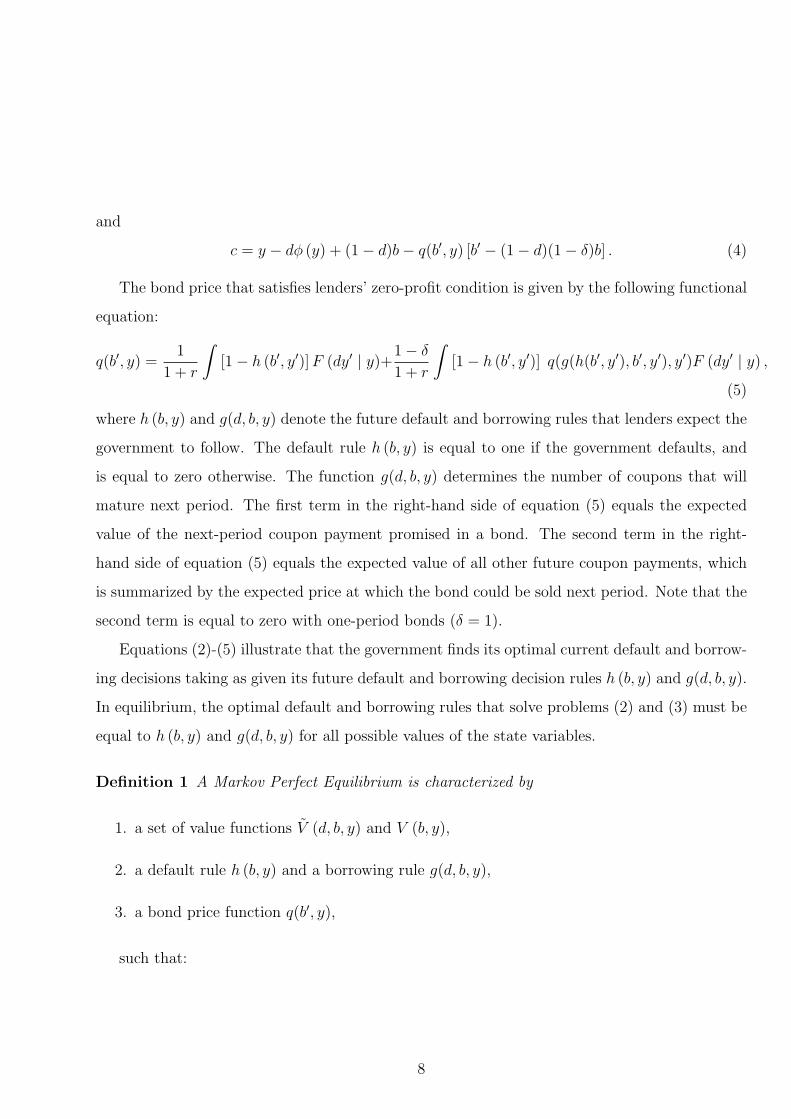
c = y − dφ (y) + (1 − d)b − q(b′, y) [b′ − (1 − d)(1 − δ)b] . (4)

The bond price that satisfies lenders’ zero-profit condition is given by the following functional

equation:

q(b′, y) =1

1 + r

∫

[1 − h (b′, y′)] F (dy′ | y)+1 − δ

1 + r

∫

[1 − h (b′, y′)] q(g(h(b′, y′), b′, y′), y′)F (dy′ | y) ,

(5)

where h (b, y) and g(d, b, y) denote the future default and borrowing rules that lenders expect the

government to follow. The default rule h (b, y) is equal to one if the government defaults, and

is equal to zero otherwise. The function g(d, b, y) determines the number of coupons that will

mature next period. The first term in the right-hand side of equation (5) equals the expected

value of the next-period coupon payment promised in a bond. The second term in the right-

hand side of equation (5) equals the expected value of all other future coupon payments, which

is summarized by the expected price at which the bond could be sold next period. Note that the

second term is equal to zero with one-period bonds (δ = 1).

Equations (2)-(5) illustrate that the government finds its optimal current default and borrow-

ing decisions taking as given its future default and borrowing decision rules h (b, y) and g(d, b, y).

In equilibrium, the optimal default and borrowing rules that solve problems (2) and (3) must be

equal to h (b, y) and g(d, b, y) for all possible values of the state variables.

Definition 1 A Markov Perfect Equilibrium is characterized by

1. a set of value functions V (d, b, y) and V (b, y),

2. a default rule h (b, y) and a borrowing rule g(d, b, y),

3. a bond price function q(b′, y),

such that:

8

(a) given h (b, y) and g(d, b, y), V (b, y) and V (d, b, y) satisfy functional equations (2) and (3)

when the government can trade bonds at q(b′, y);

(b) given h (b, y) and g(d, b, y), the bond price function q(b′, y) offered to the government

satisfies lenders’ zero-profit condition implicit in equation (5); and

(c) the default rule h (b, y) and borrowing rule g(d, b, y) solve the dynamic programming

problem defined by equations (2) and (3) when the government can trade bonds at q(b′, y).

2.2 A model without debt dilution

In the baseline model presented in Section 2.1, the debt dilution problem arises as follows.7

Note first that an increase in the current borrowing level increases the probability of a default

on previously issued debt and, thus, it decreases the market value of this debt—debt dilution

occurs. Each period, the government borrows without internalizing the cost of diluting the value

of debt issued in past periods. Lenders anticipate the effect of future borrowing on the recovery

rate of the debt they buy and require to be compensated for future debt dilutions through a

higher bond yield. Thus, the government could benefit from eliminating future debt dilutions

because this would reduce the interest rate at which it can borrow in the current period. In this

section we propose a modification to the model presented in Section 2.1 that will allow us to

study an economy without this debt dilution problem and, in turn, measure the effects of this

problem on the levels of borrowing and default risk.

In order to eliminate the debt dilution problem, we force the government to internalize the

effect of new issuances on holders of its debt. We assume that in order to issue debt the gov-

ernment must obtain permission from existing bondholders, and that the government can com-

pensate them for the dilution of the value of their debt implied by new issuances. In particular,

suppose that after the government announces how many bonds it wants to issue, it can offer

to pay a fee for each existing bond if bondholders do not oppose to the new issuances. Then,

7Bolton and Jeanne (2009) discuss how the debt dilution problem can be endogenized as the result of monitoringcosts.

9

if existing bondholders choose to approve the government’s debt issuance, the government pays

the fee and issue new bonds as in the baseline model presented in Section 2.1. Otherwise, the

government does not issue (or buyback) bonds in the current period.

As before, let q(b′, y) denote the price a sovereign bond. Let b ≡ (1 − d)(1 − δ)b denote the

interim number of next-period coupon obligations. Suppose the government issues b − b′ > 0

bonds. If the holder of a government bond chooses not to allow the government to issue new

bonds, the price of his bond would be q(b, y). Otherwise, the price would be q(b′, y) and he would

receive a fee from the government. Consequently, the minimum fee a bondholder would accept

in exchange for allowing the government to issue b − b′ bonds is q(b, y) − q(b′, y). This is the fee

the government would offer in equilibrium. Note that this imply existing bondholders make zero

profits from the government’s new issuances and, thus, is consistent with the competitive debt

market assumption of the baseline framework. The resources obtained by the government when

issuing b − b′ bonds equal (b − b′)q(b′, y) + b[q(b, y) − q(b′, y)]

It should be noticed that the resources the government obtains when issuing bonds within

the game described above are the same resources it would obtain when dealing with an exclusive

lender who makes zero profits in expectation. Suppose all government debt is held by an exclusive

who is the only one who can buy bonds from the government. If this lender choose not to buy more

debt from the government, the end-of-period value of its government’s debt holdings would be

−bq(b, y). If he buys b−b′ bonds from the government, the end-of-period value of his debt holdings

would be −b′q(b′, y). Thus, the exclusive lender is willing to buy b−b′ bonds from the government

for bq(b, y)− b′q(b′, y), which is equal to the amount the government obtains when issuing bonds

to lenders who can veto new issuances as described above ((b − b′)q(b′, y) + b[q(b, y) − q(b′, y)]).

This illustrates how the government’s borrowing opportunities with the mechanism we propose

resemble the opportunities it would have with an exclusive lender, and how one can think about

the debt dilution problem as a nonexclusivity problem.8

8A detailed analysis of how the mechanism we propose in this section could be implemented to overcomethe debt dilution problem in reality is beyond the scope of this article. However, it should be mentioned thatimplementing this mechanism may not be as difficult as one may first think. On the one hand, obtaining theapproval of all existing bondholders for new debt issuances (in exchange of a compensation to existing bondholders)may be difficult. On the other hand, asking for the approval of a representative bondholder or an institutionrepresenting the interest of bondholders could suffice. Bolton and Jeanne (2009) discuss how institutions could be

10

In addition, we assume that, as in Section 2.1, when the government wants to buyback its

bonds, it does so at the secondary-market price q(b′, y).9 Suppose the bond price is higher when

the debt level is lower because the default probability is increasing with respect to the debt level

(as we find it is the case for the parameterizations we study). The equilibrium bond price is

given by

q(b′, y) =1

1 + r

∫

[1 − h (b′, y′)] F (dy′ | y)

+1 − δ

1 + r

∫

[1 − h (b′, y′)] max {0, q(b′(1 − δ), y′) − q(g(h(b′, y′), b′, y′), y′)}F (dy′ | y)

+1 − δ

1 + r

∫

[1 − h (b′, y′)] q(g(h(b′, y′), b′, y′), y′)F (dy′ | y) . (6)

The right-hand side of equation (6) presents the components of the equilibrium bond price

without debt dilution. The first term of the right-hand side represents the expected value of next-

period coupon payment. The second term represents the compensations lenders would receive if

the government issues new debt. The existence of this compensation implies that lenders price

sovereign bonds anticipating that the value of their investment will not be diluted by new debt

issuances. The third term represents the expected next-period value of a bond.

Without the debt dilution problem, the government’s budget constraint reads

c = y−dφ (y)+(1−d)b+q(b′, y) [(1 − d)(1 − δ)b − b′]+(1−d)(1−δ)b max{0, q(b(1−δ), y)−q(b′, y)}.

(7)

The last term of the right-hand side of equation (7) represents the government’s compensation to

existing bondholders for the issuance of new debt. Replacing equations (4) and (5) by equations

(6) and (7) in the dynamic programming problem described in Section 2.1.1 give us the problem

without dilution.

assigned the task of facilitating sovereign debt restructuring. In a similar manner, institutions could be responsiblefor approving government’s proposals of new debt issuances. Requiring instead that existing bondholders donot oppose the government’s proposal may be easier. In practice, it could be required that opposition to thegovernment proposal is not too strong.

9Alternatively, we could have assume that the government receives a compensation from lenders when itbuyback debt in the same way it compensates lenders when it issues debt. That is, we could force lenders tomake transfers to the government when there is a debt buyback. Our assumption allows us to focus on the debtdilution problem discussed in the literature without introducing other modifications to the model.

11

3 Results

In this section we compare the predictions of the model with and without the modification

presented in Section 2.2. First, in order to illustrate how this modification makes the government

internalize the effect of current borrowing on the price of previous issuances, let us compare

first-order conditions that characterizes the government’s borrowing decision with and without

dilution. To simplify the notation, we do not write consumption, default, and future borrowing as

functions of the state variables. Let b ≡ (1−d)(1−δ)b denote the interim number of next-period

coupon obligations. We use fj (x1, ..., xn) to denote the first-order derivative of the function f

with respect to the argument xj. The first-order condition for the model with dilution is given

by

u1(c)q(b′, y) = β

∫

V1 (b′, y′) F (dy′ | y) − u1(c)q1(b′, y)(b′ − b). (8)

The left-hand side of equation (8) represents the marginal benefit of borrowing. By issuing

one extra bond today, the government can increase current consumption by q(b′, y) units. The

right-hand side of equation (8) represents the marginal cost of borrowing. The first term in the

right-hand side represents the “future cost of borrowing”. By borrowing more, the government

decreases expected future consumption. The second term in the right-hand side represents the

“current cost of borrowing”. By borrowing more, the government decreases the issuance price of

every bond it issues in the current period, which in turn decreases current consumption.

Suppose that, without dilution, the zero-profit bond price is decreasing in the debt level (as

we find it is for the parametrization we study) and that the government chooses to issue bonds

(b′ < b), as it is the case in every period of our simulations.10 Then, the first-order condition for

the model without dilution is given by

u1(c)q(b′, y) = β

∫

V1 (b′, y′) F (dy′ | y) − u1(c)q1(b′, y)b′. (9)

The comparison of equations (8) and (9) shows how our modification to the baseline model

allows us to eliminate the debt dilution problem. In equation (8), the debt dilution represented

10In our simulations, the government does not repurchases debt issued in previous periods (the model is simu-lated for 750,000 periods). That is, the government does not want its coupon payment obligations to decrease ata rate higher than δ = 4.5% per quarter.

12

by the change in the bond price q1(b′, y) in the “current cost of borrowing” is weighted by new

issuances (b′ − b) only. This illustrates how in the baseline model the government chooses its

issuance level without internalizing the dilution of the value of the debt held by lenders. In

contrasts, equation (9) shows that with our modification to the baseline model, the debt dilution

represented by the change in the bond price q1(b′, y) in the “current cost of borrowing” is weighted

by the entire debt stock b′. This illustrates how in the modified model the government chooses its

issuance level internalizing the dilution of the value of the debt held by lenders. This is natural

since the government has to compensate holders of its debt by the dilution of the debt value

implied by its current-period issuances. Next, we discuss the quantitative effects of the debt

dilution problem.

3.1 Parametrization

Following Hatchondo et al. (2009b), we solve the model numerically using value function iteration

and interpolation.11 Table 1 presents the parametrization we use, which is the one used in used

in Hatchondo and Martinez (2009) and is similar to the ones used in other studies of sovereign

default.

We assume a coefficient of relative risk aversion of 2, which is within the range of accepted

values in studies of real business cycles. A period in the model refers to a quarter. The risk-free

interest rate is set equal to 1%. The parameter values that govern the endowment process are

chosen so as to mimic the behavior of GDP in Argentina from the fourth quarter of 1993 to the

third quarter of 2001, following Hatchondo et al. (2009a). The parametrization of the output

process is similar to the parametrization used in other studies that consider a longer sample

period (see, for instance, Aguiar and Gopinath (2006)).

As in previous studies (see, for example, Aguiar and Gopinath (2006)), Bolton and Jeanne

11We use linear interpolation for endowment levels and spline interpolation for asset positions. The algorithmfinds two value functions, V (1, b, y) and V (0, b, y). Convergence in the equilibrium price function q(b′, y) is alsoassured. As discussed by Krusell and Smith (2003), there is typically a problem of multiplicity of Markov perfectequilibria in infinite-horizon economies. In order to avoid this problem, we solve for the equilibrium of the finite-horizon version of our economy, and we increase the number of periods of the finite-horizon economy until valuefunctions and bond prices for the first and second periods of this economy are sufficiently close. We then use thefirst-period equilibrium objects as the infinite-horizon-economy equilibrium objects.

13

Risk aversion σ 2

Interest rate r 1%

Output autocorrelation coefficient ρ 0.9

Standard deviation of innovations σǫ 2.7%

Mean log output µ (-1/2)σ2ǫ

Output loss λ 50%

Discount factor β 0.95

Duration δ 0.045

Table 1: Parameter values.

(2009), Obstfeld and Rogoff (1996), and Sachs and Cohen (1982)) we assume that the loss in

output triggered by a default is represented by a function φ (y) = λy. Hatchondo and Martinez

(2009) show that the value of λ does not significantly affect the predictions of the baseline model.

The discount factor value we assume is higher than the ones assumed in previous studies with

a cost of defaulting similar to the one in this paper (for instance, Aguiar and Gopinath (2006)

assume β = 0.8). Low discount factors may be a result of political polarization in emerging

economies (see Amador (2003) and Cuadra and Sapriza (2008)).

With δ = 4.5%, bonds have an average duration of 4.12 years in the simulations of the baseline

model. Cruces et al. (2002) report that the average duration of Argentinean bonds included in

the EMBI index was 4.13 years in 2000. This duration is not significantly different from what is

observed in other emerging economies. Using a sample of 27 emerging economies, Cruces et al.

(2002) find an average duration of 4.77 years with a standard deviation of 1.52. Hatchondo and

Martinez (2009) show that, in simulations of the baseline model, the mean and the volatility of

the spread decline monotonically when the value of δ increases.

14

3.2 Simulation results

This section discusses quantitative effects of the debt dilution problem. In order to do so, it

presents simulation results from the models with and without dilution we introduced in Sections

2.1 and 2.2, respectively. To facilitate the comparison of our results with the ones in previous

studies of sovereign default, we report results for pre-default simulation samples, as these studies

do. We simulate the model for a number of periods that allows us to extract 500 samples of 32

consecutive periods before a default. Except for the computation of default frequencies, which are

computed using all the simulation data, we focus on samples of 32 periods because we compare

the artificial data generated by the model with Argentine data from the fourth quarter of 1993

to the third quarter of 2001.12 In order to facilitate the comparison of simulation results with

the data, we only consider simulation sample paths where the last default was declared at least

two periods before the beginning of each sample.

Table 2 reports moments in the data and in our simulations.13 The moments reported in

the table are chosen so as to illustrate the ability of the model to replicate distinctive business

cycle properties of emerging economies. Relative to developed economies, emerging economies

feature higher, more volatile and countercyclical interest rate; a higher volatility of consumption

relative to income; and more countercyclical net exports. The trade balance (TB) is expressed

as a fraction of output (Y ). The interest rate spread (Rs) is expressed in annual terms.14 The

logarithm of income and consumption are denoted by y and c, respectively. The standard devi-

12The qualitative features of this data are also observed in other sample periods and in other emerging markets(see, for example, Aguiar and Gopinath (2007), Boz et al. (2008) Neumeyer and Perri (2005), and Uribe andYue (2006)). The only exception is that in the data we consider, the volatility of consumption is slightly lowerthan the volatility of income, while emerging market economies tend to display a higher volatility of consumptionrelative to income.

13The data for output, consumption, and trade balance were obtained from the Argentinean Finance Ministry.The spread before the first quarter of 1998 is taken from Neumeyer and Perri (2005), and from the EMBI Globalafter that. We do not report the debt level and the default frequency in the data because, as argued in Hatchondoand Martinez (2009), we believe that debt levels generated by the baseline model of sovereign default are difficultto compare with debt levels in the data, and that it is difficult to obtain a precise measure of default frequencies.

14Let

r∗ =1

q(b′, y)− δ

denote the per-period constant yield implied by a bond price q(b′, y). The annualized spread is given by Rs =(

1+r∗

1+r

)4

− 1.

15

ation of x is denoted by σ (x) and is reported in percentage terms. The coefficient of correlation

between x and z is denoted by ρ (x, z). Moments are computed using detrended series. Trends

are computed using the Hodrick-Prescott filter with a smoothing parameter of 1, 600.

Data With Without δ = 1

dilution dilution

Debt/output 0.51 0.45 0.44

Defaults per 100 years 2.72 0.01 0.12

E(Rs) 7.44 2.73 0.01 0.12

σ (Rs) 2.51 0.33 0.01 0.06

σ(y) 3.17 3.07 3.05 3.15

σ(c) 2.98 3.45 3.54 3.66

σ (TB/Y ) 1.35 0.56 0.79 0.85

ρ (c, y) 0.97 0.99 0.98 0.98

ρ (TB/Y, y) -0.69 -0.64 -0.53 -0.50

ρ (Rs, y) -0.65 -0.86 -0.73 -0.77

ρ (Rs, TB/Y ) 0.56 0.88 0.86 0.93

Table 2: Business cycle statistics. The second column is computed using data from Argentina from1993 to 2001. Other columns report the mean of the value of each moment in 500 simulation samples.

Table 2 shows that simulations of our baseline model, as the ones of models used in recent

studies, generate a mean and standard deviation of the spread that are lower than their data

counterpart. This is not surprising since, as most previous studies, we assume risk-neutral lenders

while it has been documented that the risk premium is an important component of sovereign

spreads and that most of the spread volatility in the data is accounted for by volatility in the risk

premium (see, for example, Borri and Verdelhan (2009), Broner et al. (2007), Longstaff et al.

(2009), and Gonzalez-Rozada and Levy Yeyati (2008)). Arellano (2008) and Lizarazo (2005,

2006) show that the mean and the standard deviation of the spread generated by a default model

can be increased by assuming risk-averse lenders. Table 2 also shows that in our simulations, as

16

in the ones in previous studies and in the data, consumption and income are highly correlated,

the consumption volatility is higher than the income volatility, and spread and trade balances

are countercyclical. Overall, we believe that the simulations of our benchmark with dilution

matches the data at least as well as the simulations in previous studies. With this in mind, we

concentrate on the main question this paper intends to answer: what are the quantitative effects

of the debt dilution problem?

The comparison of the simulation results obtained with and without dilution show that dilu-

tion accounts for 12% of the mean debt level in the simulations of the baseline model. Further-

more, eliminating dilution decreases the mean spread in the simulations from 2.73% to 0.01%.

That is, dilution accounts for almost 100% of the spread paid by the government. Since we

assume risk-neutral lenders, the default frequency in the simulation resembles the mean spread.

The number of default per 100 years decreases from 2.72 in the baseline to 0.01 without debt

dilution. The standard deviation of the spread decreases from 0.33 with debt dilution to 0.01

without debt dilution. Thus, when the government overcomes the debt dilution problem, it never

chooses to take significant default risk.

In order to shed more light on how the debt dilution problem influences equilibrium alloca-

tions, Figure 1 presents the combination of spread levels and face value of next-period debt—

defined as the present value of future payment obligations discounted at the risk-free rate, b′

δ+r—

chosen by the government. The figure also presents the spread that renders lenders zero profits

in expectation as a function of the face value of next-period debt—this is the set of combinations

of spreads and next-period debt levels that the government can choose from.

For the baseline model, the left panel of Figure 1 illustrates how the government cannot

borrow paying spreads close to zero. Even if the government chooses low debt levels, spread

levels would be substantially above zero. For low debt levels, the probability of a default in

the next period is close to zero. However, the expected recovery rate—i.e., the fraction of the

loan lenders expect to recover—is significantly away from one because lenders anticipate positive

default probabilities in future periods. For instance, the left panel of Figure 1 shows that, as one

would expect, the government chooses to take significant default risk (i.e., to pay high spreads) in

bad times, when it needs to borrow more. Suppose, for example, that the government is issuing

17

−0.6 −0.5 −0.4 −0.3 −0.2 −0.1 00

1

2

3

4

q scheme and optimum at the avg b in the simulations

Debt

An

nu

al

sp

read

(%

)

−0.6 −0.5 −0.4 −0.3 −0.2 −0.1 0

Figure 1: Menu of combinations of spreads and next-period debt levels ( b′

δ+r) from which the government

can choose. The left panel corresponds to the baseline model. The center panel corresponds to the modelwith compensations to bondholders for debt dilution. The right panel corresponds to the one-period-bond model. In each case, solid dots illustrate the optimal decision of a government that inherits a debtlevel equal to the average debt observed in our simulations for that case. The low (high) value of y

corresponds to an endowment realization that is one standard deviation below (above) the unconditionalmean.

debt for the first time. No matter how small the first issuance is, lenders would anticipate an

expected recovery rate lower than one because they can forecast future issuance behavior. This

implies that the government does not have the choice to issue small amounts at the risk-free rate.

In contrast, the center panel of Figure 1 illustrates how eliminating the debt dilution problem

gives the government the opportunity to borrow paying spreads close to zero. The figure shows

that, even in bad times, the government will choose to keep the default probability close to

zero and, therefore, to pay spreads close to zero. The intuition behind this finding is straight-

forward. One may think about the government as choosing the default probability in each

period—choosing to issue more debt is equivalent to choosing a higher default probability. The

government’s commitment to compensating bondholders for any debt dilution it creates reduces

incentives to choose higher default probabilities in bad times because this would imply com-

pensating bondholders for the corresponding dilution in their bonds value. In our quantitative

exercise, the government never wants to pay significant compensations to bondholders.

18

3.2.1 One-period bonds vs. long bonds without debt dilution

Table 2 also presents simulation results obtained assuming one-period bonds (δ = 1). The one-

period bond assumption is commonly used in studies of sovereign default. With this assumption,

there is no room for debt dilution because when the government decides its borrowing level, the

outstanding debt level is zero (either because the government honored its debt obligations at the

beginning of the period or because it defaulted on them. Hatchondo and Martinez (2009) show

that the mean and the standard deviation in the simulations of the baseline model increase as

the assumed duration of sovereign bonds increases (see also Chatterjee and Eyigungor (2009)).

The comparison of the results obtained with one-period bonds and the ones obtained when

the government can commit indicate the debt dilution problem accounts for more than 100%

of the increase in the mean and standard deviation of the spread discussed by Hatchondo and

Martinez (2009). That is, the mean and the standard deviation of the spread are lower when the

government compensates bondholders for debt dilution than with one-period bonds.

Why are equilibrium spread levels higher and more volatile with one-period bonds than with

long-bonds without dilution? In spite of debt dilution not being and issue with either one-period

bonds or long-bonds without dilution, these are two different assets. Recall that, in models of

sovereign default, the negative impact of a bad income shock in the government’s borrowing

constraint is amplified through its indirect effect on the set of borrowing levels and spreads

available to the government (see, for example, the spread functions in Figure 1). Even without

dilution, long bonds continue to provide insurance against the effect of endowment shocks in the

government’s borrowing cost. Recall that we assume that lenders are compensated for the effect

of new issuances in bond prices, but not for declines in the bond price implied by the worsening

of economic conditions. The comparison of the center and right panels of Figure 1 shows us that,

with one period bonds, the government chooses to pay significantly higher spreads in bad times

than in good times. This does not occur when the government compensates bondholders for debt

dilution. With one-period bonds, the indirect effect of a bad income shock in the government’s

borrowing opportunities is more severe because the government has to issue its entire desired

debt stock. This does not occur with long-duration bonds. The longer the duration of bonds

19

(i.e., the smaller the fraction of its debt the government would need to rollover to maintain a

constant debt level), the more protected the government is against the effect of a negative income

shock on the cost of borrowing. This makes the government’s borrowing needs after encountering

a bad income shock larger in the one-period-bond version of the model than in the model with

long bonds and without dilution.

4 Conclusions and extensions

We proposed an extension of a baseline sovereign default framework a la Eaton and Gersovitz

(1981) that allowed us to study the case in which the sovereign eliminates the overborrowing

implied by debt dilution. The comparison of the results obtained without dilution and the

ones obtained with the baseline framework (where dilution occurs) allowed us to measure the

overborrowing implied by dilution and its consequences for default risk. We found that dilution

accounts for almost 100% of the default risk in the simulations of the baseline model. That is,

even without commitment to future repayment policies and without contingency of sovereign

debt, if the sovereign could eliminate the dilution problem, it would almost eliminate default

risk.

The default risk implied by the debt dilution problem is reflected in higher interest rate

spreads for sovereign bonds. For emerging economies, previous studies find evidence of a sig-

nificant effect of interest rate spreads on productivity (through the allocation of factors of pro-

duction), and of a significant role of interest rate spreads in the amplification of shocks to these

economies (see, for example, Mendoza and Yue (2008), Neumeyer and Perri (2005), and Uribe

and Yue (2006)). In the light of these findings, our results indicate that the welfare cost of the

overborrowing implied by debt dilution may be large. Thus, for countries that pay high sovereign

spreads, it may be worth exploring the possibility of committing to rules that attenuate the over-

borrowing generated by debt dilution.

The baseline model of sovereign default focuses on an economy without production in which

interest rates cannot affect productivity. Thus, this model is ill-suited for studying the welfare

cost of the debt dilution problem. The developing of a sovereign default framework that ac-

20

commodates effects of interest rates on productivity is the subject of ongoing research (see, for

example, Mendoza and Yue (2008)). An interesting extension of our analysis would be to study

the implications of the debt dilution problem in such a framework and evaluate the welfare cost

of this problem. Furthermore, one could use such framework to measure the effect of the debt

dilution problem on the business cycle properties of the model economy.

Ongoing research also highlights the importance of the risk premium in sovereign bonds’

spreads and incorporates risk-averse lenders into the baseline sovereign default framework (see,

for example, Arellano (2008), Borri and Verdelhan (2009), Broner et al. (2007), Lizarazo (2005,

2006), Longstaff et al. (2009), and Gonzalez-Rozada and Levy Yeyati (2008)). Incorporating

risk-averse lenders into the baseline model is challenging, complicates the analysis, and may

make our results less transparent. Nevertheless, it would be interesting how our measurement of

the effects of debt dilution is affected by lenders’ risk aversion.

21

References

Aguiar, M. and Gopinath, G. (2006). ‘Defaultable debt, interest rates and the current account’.

Journal of International Economics , volume 69, 64–83.

Aguiar, M. and Gopinath, G. (2007). ‘Emerging markets business cycles: the cycle is the trend’.

Journal of Political Economy , volume 115, no. 1, 69–102.

Alfaro, L. and Kanczuk, F. (2005). ‘Sovereign debt as a contingent claim: a quantitative ap-

proach’. Journal of International Economics , volume 65, 297 314.

Amador, M. (2003). ‘A Political Economy Model of Sovereign Debt Repayment’. Manuscript,

Stanford University.

Arellano, C. (2008). ‘Default Risk and Income Fluctuations in Emerging Economies’. American

Economic Review , volume 98(3), 690–712.

Arellano, C. and Ramanarayanan, A. (2008). ‘Default and the Maturity Structure in Sovereign

Bonds’. Mimeo, University of Minnesota.

Athreya, K. (2002). ‘Welfare Implications of the Bankruptcy Reform Act of 1999’. Journal of

Monetary Economics , volume 49, 1567–1595.

Athreya, K., Tam, X. S., and Young, E. R. (2007a). ‘Does Rising Income Risk Lead to Better

Risk Sharing?’ Manuscript, University of Virginia.

Athreya, K., Tam, X. S., and Young, E. R. (2007b). ‘A Quantitative Model of Information and

Unsecured Lending’. Manuscript, University of Virginia.

Bai, Y. and Zhang, J. (2006). ‘Financial integration and international risk sharing’. Working

Paper, Michigan University.

Benjamin, D. and Wright, M. L. J. (2008). ‘Recovery Before Redemption? A Theory of Delays

in Sovereign Debt Renegotiations’. Manuscript.

22

Bi, R. (2006). ‘Debt Dilution and the Maturity Structure of Sovereign Bonds’. Manuscript,

University of Maryland.

Bizer, D. S. and DeMarzo, P. (1992). ‘Sequential Banking’. Journal of Political Economy , volume

100, 41–61.

Bolton, P. and Jeanne, O. (2009). ‘Structuring and Restructuring Sovereign Debt: The Role of

Seniority’. Review of Economic Studies , volume 76, 879902.

Borensztein, E., Chamon, M., Jeanne, O., Mauro, P., and Zettelmeyer, J. (2004). ‘Sovereign

Debt Structure for Crisis Prevention’. IMF occasional paper 237.

Borensztein, E. and Mauro, P. (2004). ‘The case for GDP-indexed bonds’. Economic Policy ,

volume 38, 167–216.

Borri, N. and Verdelhan, A. (2009). ‘Sovereign Risk Premia’. Boston University.

Boz, E. (2009). ‘Sovereign Default, Private Sector Creditors, and the IFIs’. Umpublished

manuscript.

Boz, E., Daude, C., and Durdu, B. (2008). ‘Emerging Market Business Cycles Revisited: Learning

about the Trend’. Board of Governors International Finance Discussion Papers No. 927.

Broner, F. A., Lorenzoni, G., and Schmukler, S. L. (2007). ‘Why do emerging economies borrow

short term?’ National Bureau of Economic Research Working Paper 13076.

Chatterjee, S., Corbae, D., Nakajima, M., and Rıos-Rull, J.-V. (2007a). ‘A Quantitative Theory

of Unsecured Consumer Credit with Risk of Default’. Econometrica, volume 75, 1525–1589.

Chatterjee, S., Corbae, D., and Rıos-Rull, J.-V. (2007b). ‘Credit Scoring and Competitive Pricing

of Default Risk’. Manuscript, University of Texas at Austin.

Chatterjee, S. and Eyigungor, B. (2009). ‘Maturity, Indebtedness and Default Risk’. Federal

Reserve Bank of Philadelphia Working Paper 09-02.

23

Cole, H., Dow, J., and English, W. (1995). ‘Default, settlement, and signaling: lending resump-

tion in a reputational model of sovereign debt’. International Economic Review , volume 36,

no. 2, 365–385.

Copeland, T. E. and Weston, J. F. (1992). Financial theory and corporate policy . Addison-Wesley

Publishing Company.

Cruces, J. J., Buscaglia, M., and Alonso, J. (2002). ‘The Term Structure of Country Risk and

Valuation in Emerging Markets’. Manuscript, Universidad Nacional de La Plata.

Cuadra, G., Sanchez, J. M., and Sapriza, H. (forthcoming). ‘Fiscal policy and default risk in

emerging markets’. Review of Economic Dynamics .

Cuadra, G. and Sapriza, H. (2006). ‘Sovereign default, terms of trade, and interest rates in

emerging markets’. Working Paper 2006-01, Banco de Mexico.

Cuadra, G. and Sapriza, H. (2008). ‘Sovereign default, interest rates and political uncertainty in

emerging markets’. Journal of International Economics , volume 76, 7888.

D’Erasmo, P. (2008). ‘Government Reputation and Debt Repayment in Emerging Economies’.

Manuscript, University of Texas at Austin.

Detragiache, E. (1994). ‘Sensible buybacks of sovereign debt’. Journal of Development Eco-

nomics , volume 43, 317–333.

Durdu, C. B. (2009). ‘Quantitative implications of indexed bonds in small open economies’.

Journal of Economic Dynamics Control , volume 33, 883902.

Eaton, J. and Gersovitz, M. (1981). ‘Debt with potential repudiation: theoretical and empirical

analysis’. Review of Economic Studies , volume 48, 289–309.

Gonzalez-Rozada, M. and Levy Yeyati, E. (2008). ‘Global factors and emerging market spreads’.

Economic Journal , volume 118, 19171936.

24

Guembel, A. and Sussman, O. (2009). ‘Sovereign Debt without Default Penalties’. Review of

Economic Studies , volume 76, 1297–1320.

Hatchondo, J. C. and Martinez, L. (2007). ‘Credit risk without commitment’. Unpublished

manuscript.

Hatchondo, J. C. and Martinez, L. (2009). ‘Long-duration bonds and sovereign defaults’. Journal

of International Economics , volume 79, 117–125.

Hatchondo, J. C., Martinez, L., and Sapriza, H. (2007). ‘Quantitative Models of Sovereign

Default and the Threat of Financial Exclusion’. Economic Quarterly , volume 93, 251–286.

No. 3.

Hatchondo, J. C., Martinez, L., and Sapriza, H. (2009a). ‘Heterogeneous borrowers in quantita-

tive models of sovereign default.’ International Economic Review , volume 50, 1129 – 1151.

Hatchondo, J. C., Martinez, L., and Sapriza, H. (2009b). ‘On the Cyclicality of the Interest Rate

in Emerging Economy Models: Solution Methods Matter’. Working Paper No. 09-13. Federal

Reserve Bank of Richmond.

Kletzer, K. M. (1984). ‘Asymmetries of Information and LDC Borrowing with Sovereign Risk’.

The Economic Journal , volume 94, 287–307.

Krusell, P. and Smith, A. (2003). ‘Consumption-savings decisions with quasi-geometric discount-

ing’. Econometrica, volume 71, no. 1, 365–375.

Li, W. and Sarte, P.-D. (2006). ‘U.S. consumer bankruptcy choice: The importance of general

equilibrium effects’. Journal of Monetary Economics , volume 53, 613–631.

Livshits, I., MacGee, J., and Tertilt, M. (2008). ‘Consumer Bankruptcy: A Fresh Start,’. Amer-

ican Economic Review , volume 97, 402–418.

Lizarazo, S. (2005). ‘Sovereign risk and risk averse international investors’. Working Paper,

ITAM.

25

Lizarazo, S. (2006). ‘Contagion of financial crises in sovereign debt markets’. Working Paper,

ITAM.

Longstaff, F. A., Pan, J., Pedersen, L. H., and Singleton, K. J. (2009). ‘HOW SOVEREIGN IS

SOVEREIGN CREDIT RISK?’ UCLA Working Paper.

Mendoza, E. and Yue, V. (2008). ‘A Solution to the Default Risk-Business Cycle Disconnect’.

Manuscript, New York University.

Neumeyer, P. and Perri, F. (2005). ‘Business cycles in emerging economies: the role of interest

rates’. Journal of Monetary Economics , volume 52, 345–380.

Niepelt, D. (2008). ‘Debt Maturity without Commitment’. Manuscript, Study Center Gerzensee.

Obstfeld, M. and Rogoff, K. (1996). ‘Foundations of International Macroeconomics’. Cam-

bridge,MA: MIT Press.

Sachs, J. and Cohen, D. (1982). ‘LDC borrowing with default risk’. National Bureau of Economic

Research Working Paper 925.

Sanchez, J. M. (2008). ‘The Role of Information in Consumer Debt and Bankruptcy’. Manuscript,

University of Rochester.

Sandleris, G., Sapriza, H., and Taddei, F. (2009). ‘Indexed Sovereign Debt: An Applied Frame-

work’. Universidad Torcuato Di Tella Working Paper 01/2009.

Tirole, J. (2002). ‘Financial Crises, Liquidity, and the International Monetary System’. Princeton

University Press.

Tomz, M. and Wright, M. L. J. (2007). ‘Do Countries Default in “Bad Times”?’ Journal of the

European Economic Association, volume 5, 352–360.

Uribe, M. (2006a). ‘Individual Versus Aggregate Collateral Constraints and the Overborrowing

Syndrome’. NBER working paper No. 12260.

26

Uribe, M. (2006b). ‘On Overborrowing’. American Economic Review Papers and Proceedings ,

volume 96, 417–421.

Uribe, M. and Yue, V. (2006). ‘Country spreads and emerging countries: Who drives whom?’

Journal of International Economics , volume 69, 6–36.

Yue, V. (2005). ‘Sovereign default and debt renegotiation’. Working Paper, NYU.

27