Quantitative properties of sovereign default models: Solution methods matter

Working Paper Series

This paper can be downloaded without charge from: http://www.richmondfed.org/publications/economic_research/working_papers/index.cfm

http://www.richmondfed.org/publications/economic_research/working_papers/index.cfm

Quantitative properties of sovereign default models:

solution methods matter∗

Juan Carlos Hatchondo† Leonardo Martinez‡ Horacio Sapriza§

Federal Reserve Bank of Richmond Working Paper No. 10-04

March 26, 2010

Abstract

We study the sovereign default model that has been used to account for the cyclicalbehavior of interest rates in emerging market economies. This model is often solved usingthe discrete state space technique with evenly spaced grid points. We show that thismethod necessitates a large number of grid points to avoid generating spurious interestrate movements. This makes the discrete state technique significantly more inefficientthan using Chebyshev polynomials or cubic spline interpolation to approximate the valuefunctions. We show that the inefficiency of the discrete state space technique is more severefor parameterizations that feature a high sensitivity of the bond price to the borrowing levelfor the borrowing levels that are observed more frequently in the simulations. In addition,we find that the efficiency of the discrete state space technique can be greatly improvedby (i) finding the equilibrium as the limit of the equilibrium of the finite-horizon versionof the model, instead of iterating separately on the value and bond price functions and (ii)concentrating grid points in asset levels at which the bond price is more sensitive to theborrowing level and in levels that are observed more often in the model simulations. Ouranalysis is also relevant for the study of other credit markets.

JEL classification: F34, F41.Keywords: Emerging economies, sovereign debt, default, numerical methods.

∗For comments and suggestions, we thank Huberto Ennis, Per Krusell, Enrique Mendoza, and our colleagues atthe Federal Reserve Bank of Richmond. We thank Cristina Arellano, Mark Aguiar and Gita Gopinath for makingavailable the codes used for Arellano (2008) and Aguiar and Gopinath (2006). We also thank Brian Gaines andElaine Mandaleris-Preddy for editorial support. Remaining mistakes are our own. The views expressed hereinare those of the authors and should not be attributed to the IMF, its Executive Board, or its management, theFederal Reserve Bank of Richmond, or the Board of Governors of the Federal Reserve System.

†Federal Reserve Bank of Richmond; e-mail: [email protected].‡IMF & Federal Reserve Bank of Richmond; e-mail: [email protected].§Federal Reserve Board of Governors and Rutgers University, e-mail: [email protected].

1 Introduction

Business cycles in small emerging economies differ from those in developed economies. Emerging

economies feature higher, more volatile and countercyclical interest rates, higher output volatility,

more countercyclical net exports, and higher consumption volatility relative to income volatility

(see, for example, Aguiar and Gopinath (2007), Neumeyer and Perri (2005), and Uribe and Yue

(2006)). The behavior of the domestic interest rate is considered an important factor that may

account for these features (see, for example, Benjamin and Meza (2009), Neumeyer and Perri

(2005), and Uribe and Yue (2006)). Thus, a state-dependent interest rate schedule is commonly

used in emerging economy models. Some studies assume an exogenous interest rate schedule.1 In

contrast, models of sovereign default provide microfoundations for the interest rate schedule based

on the risk of default. Aguiar and Gopinath (2006) and Arellano (2008) were the first studies

to extended the model in Eaton and Gersovitz (1981) and used it for the analysis of business

cycles in emerging economies.2 The model studied by Aguiar and Gopinath (2006) and Arellano

(2008) needs to be solved using numerical methods. We show how the simulated behavior of the

interest rate generated by the model can be significantly affected by approximation errors and

discuss the performance of different numerical methods.

Aguiar and Gopinath (2006) and Arellano (2008) consider a small open economy that re-

ceives a stochastic endowment stream of a single tradable good. The government’s objective

is to maximize the expected utility of private agents. Each period, the government makes two

decisions. First, it decides whether to default on previously issued debt. Second, it decides how

much to borrow or save. The government can borrow (save) by issuing (buying) one-period non-

contingent bonds that are priced in a competitive market inhabited by risk-neutral investors.

The cost of defaulting is given by an endowment loss and exclusion from capital markets.

1See, for example, Aguiar and Gopinath (2007), Neumeyer and Perri (2005), Schmitt-Grohe and Uribe (2003),and Uribe and Yue (2006).

2The model analyzed in Aguiar and Gopinath (2006) and Arellano (2008) has been extended in variousdimensions. See, for example, Cuadra et al. (forthcoming), Cuadra and Sapriza (2008), Hatchondo and Martinez(2009), and Hatchondo et al. (2007, 2009). The model used in these studies also share blueprints with the modelsused in quantitative studies of household bankruptcy—see, for example, Athreya (2002), Chatterjee et al. (2007),Li and Sarte (2006), and Livshits et al. (2008).

1

Aguiar and Gopinath (2006) and Arellano (2008) solve the model using the discrete state

space technique (hereafter referred to as DSS), which is also used in several other default studies.

That is, they discretize the stochastic process for the endowment and restrict the sovereign to

choose the optimal borrowing level from a discrete set of points. We solve the model using

DSS with different grid specifications and using two interpolation methods: one approximates

the value functions as the sum of Chebyshev polynomials and the other one approximates them

using cubic splines. Using interpolation methods enables us to let the sovereign choose its optimal

borrowing level from a continuous set and to allow for endowment realizations that do not lie on

the grid.

While the potential for DSS approximation errors to influence simulation results is a theo-

retical possibility, it has not been established whether these errors may be significant enough

to misguide the conclusions of the research agenda. We find that, to generate reliable results,

the DSS technique requires a significantly larger number of grid points than the ones used in

Aguiar and Gopinath (2006) and Arellano (2008). For instance, the standard deviation of the

interest rate spread (the difference between the yields of government bonds and the yields of

US government bonds) in the simulations of the model is less than half of the values they re-

port. In addition, when we solve Aguiar and Gopinath (2006) using more accurate methods,

the correlation between the spread and income is around -0.6 in their parameterization with

shocks to the income level and 0.1 in their parameterization with shocks to the growth rate of

income. In contrast, Aguiar and Gopinath (2006) report that this correlation is 0.5 in the first

parameterization and -0.03 in the second one. Thus, our results cast doubt on their conclusion

that income processes with shocks to the growth rate help models of sovereign default generate

a countercyclical interest rate and, therefore, help replicate the positive correlation between the

interest rate and the current account observed in the data.3

We report the relative performance of different numerical methods. We show that we are able

3As explained by Aguiar and Gopinath (2006), shocks to the growth rate of income tend to make the bondprice schedule that delivers zero expected profits less sensitive to the borrowing level. This could help generatemore countercyclical spreads. However, we find that this effect is not significant when the government alwayschooses borrowing levels very close to those for which lenders charge the risk-free interest rate (as occurs in theirsimulations).

2

to obtain robust results using cubic spline interpolation and Chebyshev collocation, and that the

results obtained using DSS converge toward the ones obtained using interpolation methods as the

number of DSS grid points increases. We find that using DSS with evenly spaced grid points (as

done in most default studies) is significantly more inefficient than using interpolation methods.

For instance, when solving the model for one of the parameterizations in Aguiar and Gopinath

(2006), it takes less than 20 minutes to find a solution that is not affected by spurious spread

volatility when the model is solved using cubic splines. It takes over 45 hours to find such a

solution using DSS with evenly spaced grid points.

Our findings also indicate that DSS inefficiencies are less significant for parameterizations

of the model that display a bond price function that is less sensitive to the borrowing level.

Thus, DSS inefficiencies are less severe when the economy is assumed to be hit with shocks to

the growth rate of income and even less so when the parameterization of the output cost of

defaulting coincides with the one in Arellano (2008).4 This indicates that the efficiency of DSS

can be improved by using grids for asset levels that concentrate points at levels for which the

bond price is more sensitive to the borrowing level and at levels that are observed more often

in the model simulations. We show this is true for the model studied in Aguiar and Gopinath

(2006) and Arellano (2008).

In addition, we document that the DSS computation time can be decreased significantly by

using a one-loop algorithm that iterates simultaneously on the value and the bond price functions

instead of using an algorithm with two loops: one for the value functions and one for the bond

price function. For example, we find that using DSS with a one-loop algorithm takes 31 seconds

to solve for the baseline model in Arellano (2008), while using the two-loop algorithm takes 182

seconds. The comparison was performed using the convergence criteria and grid specifications

that replicate her results. That difference in computation time would become more significant

if one wanted to use the simulated method of moments to calibrate the model (as Arellano 2008

and many other default studies do) or if one wanted to use finer grids to mitigate approximation

4The main difference between the parameterizations in Aguiar and Gopinath (2006) and Arellano (2008)is that in Arellano (2008), the default punishment can be significantly more responsive to current endowmentrealizations. This feature helps reduce the sensitivity of the bond price to the borrowing level.

3

errors.

Even though our analysis focuses on the model studied by Aguiar and Gopinath (2006) and

Arellano (2008), our findings may be relevant for other extensions of the baseline model. For

example, we find that it is computationally costly to eliminate the significant distortions that

DSS introduces in the behavior of the interest rate spread for the models presented in Hatchondo

and Martinez (2009) and Hatchondo et al. (2007, 2009). Our analysis is also significant for the

study of other credit markets. In quantitative studies of default, computation power is often a

binding constraint that limits researchers’ ability to study more interesting frameworks.

The rest of the article proceeds as follows. Section 2 presents the model. Section 3 presents

the parameterization we use. Section 4 discusses the computation. Section 5 presents the results

we obtain with DSS and interpolation methods. Section 6 discusses the robustness of the results

reported in Aguiar and Gopinath (2006) and Arellano (2008). Section 7 concludes.

2 The Model

We solve the model studied by Aguiar and Gopinath (2006) and Arellano (2008). They consider

a small open economy that receives a stochastic endowment stream of a single tradable good.

The endowment yt may be hit by a transitory and a permanent shock. Namely,

yt = AeztΓt,

where A is a constant, zt is the current realization of the transitory component, and Γt denotes

the current realization of the permanent component.

The variable zt follows an AR(1) process with long-run mean µz and autocorrelation coefficient

|ρz| < 1:

zt = (1 − ρz)µz + ρzzt−1 + εzt ,

where εzt ∼ N (0, σ2

z).

4

The stochastic process of the permanent component is represented by

Γt = gtΓt−1,

where gt denotes the trend shock and

ln (gt) = (1 − ρg) (ln (µg) −m) + ρgln (gt−1) + εt,

with |ρg| < 1, εt ∼ N(

0, σ2g

)

, and m = 12

σ2g

1−ρ2g.

The government’s objective is to maximize the expected present discounted value of the

representative agent’s future utility. The representative agent has CRRA preferences over con-

sumption:

u (c) =c1−γ − 1

1 − γ,

where γ denotes the coefficient of relative risk aversion.

The government makes two decisions in every period. First, it decides whether to refuse to

pay previously issued debt. Defaults imply a total repudiation of government debt. Second, the

government decides how much to borrow or save for the following period.

Aguiar and Gopinath (2006) and Arellano (2008) assume that there are two costs of defaulting.

First, the country is excluded from capital markets. In each period after the default period, the

country regains access to capital markets with probability ψ ∈ [0, 1]. Second, if a country has

defaulted on its debt, it faces an “output loss” of φ (y) in every period in which it is excluded

from capital markets.

The government can choose to save or borrow using one-period bonds. The bond price is

determined as follows. First, the government announces how many bonds it wants to issue—

each bond consists of a promise to deliver one unit of the good in the next period. Then, foreign

lenders offer a price at which they are willing to purchase these bonds. Finally, the government

sells the bonds to the lenders who offer the highest price. Lenders can borrow or lend at the risk-

free rate r, are risk neutral, and have perfect information regarding the economy’s endowment.

Let b denote the government’s current position in bonds. A negative value of b denotes that the

country was an issuer of bonds in the previous period. In equilibrium, lenders offer a price

5

q (b′, z,Γ, g) =1

1 + r

[

1 −

∫ ∫

d (b′, z′, g′Γ, g′)FZ (dz′ | z)FG (dg′ | g)

]

(1)

that satisfies their zero-profit condition when the government issues b′ bonds, and the optimal

default rule is represented by the indicator function d (b, z,Γ, g). The default rule takes a value

of 1 if it is optimal for the government to default, and takes a value of 0 otherwise.

Let FZ and FG denote the cumulative distribution functions for z and g. The value function

of a sovereign that has access to financial markets is given by

V (b, z,Γ, g) = maxd∈{0,1}

{(1 − d)V0 (b, z,Γ, g) + dV1 (z,Γ, g)} , (2)

where

V1 (z,Γ, g) = u (y − φ(y))+β

∫ ∫

[ψV (0, z′, g′Γ, g′) + (1 − ψ)V1(z′, g′Γ, g′)]FZ (dz′ | z)FG (dg′ | g)

(3)

denotes the value function of an excluded sovereign, and

V0 (b, z,Γ, g) = maxb′

{

u (y + b− q (b′, z,Γ, g) b′) + β

∫ ∫

V (b′, z′, g′Γ, g′)FZ (dz′ | z)FG (dg′ | g)

}

(4)

denotes the Bellman equation when the sovereign has decided to pay back its debt.

Definition 1 A recursive equilibrium consists of the following elements:

1. A set of value functions V (b, z,Γ, g), V1 (z,Γ, g), and V0 (b, z,Γ, g);

2. A set of policies for asset holdings b′ (b, z,Γ, g) and default decisions d (b, z,Γ, g); and

3. A bond price function q (b′, z,Γ, g), such that

(a) V (b, z,Γ, g), V1 (z,Γ, g), and V0 (b, z,Γ, g) satisfy functional equations (2), (3), and

(4), respectively;

(b) the default policy d (b, z,Γ, g) solves problem (2), and the policy for asset holdings

b′ (b, z,Γ, g) solves problem (4); and

(c) the bond price function q (b′, z,Γ, g) is given by equation (1).

6

3 Parameterization

We solve the model for three parameterizations. The first two parameterizations are the ones

considered by Aguiar and Gopinath (2006), who assume that φ (y) = λy. The third parameteri-

zation is the one considered by Arellano (2008), who assumes that

φ (y) =

y − λ if y > λ

0 if y ≤ λ.(5)

The first two parameterizations correspond to Model I and Model II in Aguiar and Gopinath

(2006). The first one corresponds to the case in which the economy is hit only with transitory

shocks to the endowment level. The second one corresponds to the case in which the economy

is hit only with shocks to the growth rate of income. The case considered in Arellano (2008) is

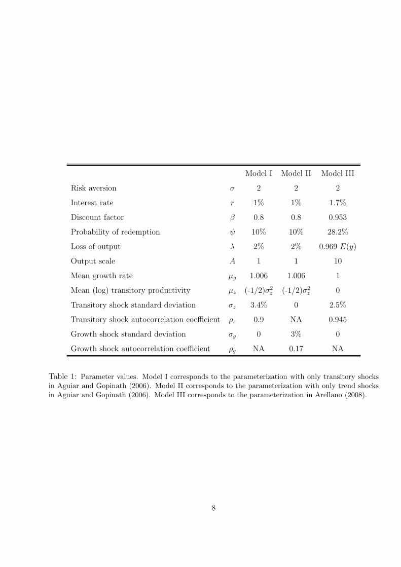
denoted as Model III. Each period corresponds to a quarter. Parameter values are specified in

Table 1.

4 Computation

We solve the model numerically using value function iteration. The algorithms find the value

functions V0 and V1. Following Aguiar and Gopinath (2006), we recast the Bellman equations in

de-trended form in order to find the solutions for Models I and II. In those cases, all variables are

normalized by µgyt−1. Since the government’s objective function may not be globally concave,

when we solve the model using interpolation methods, we first find a candidate value for the

optimal borrowing level using a global search procedure. That candidate value is then used as

an initial guess in a non-linear optimization routine. When using interpolation methods, we

use a first-order Taylor approximation to evaluate the value functions at endowment and asset

levels outside the grids. Following previous default studies, we do not extrapolate when we use

DSS. A more detailed explanation of the algorithm is presented in the appendix. Codes were

compiled using Fortran 90 and were run in serial mode on a Unix platform using Intel Xeon 5160

processors with a speed of 3.0 GHz.

7

Model I Model II Model III

Risk aversion σ 2 2 2

Interest rate r 1% 1% 1.7%

Discount factor β 0.8 0.8 0.953

Probability of redemption ψ 10% 10% 28.2%

Loss of output λ 2% 2% 0.969 E(y)

Output scale A 1 1 10

Mean growth rate µg 1.006 1.006 1

Mean (log) transitory productivity µz (-1/2)σ2z (-1/2)σ2

z 0

Transitory shock standard deviation σz 3.4% 0 2.5%

Transitory shock autocorrelation coefficient ρz 0.9 NA 0.945

Growth shock standard deviation σg 0 3% 0

Growth shock autocorrelation coefficient ρg NA 0.17 NA

Table 1: Parameter values. Model I corresponds to the parameterization with only transitory shocksin Aguiar and Gopinath (2006). Model II corresponds to the parameterization with only trend shocksin Aguiar and Gopinath (2006). Model III corresponds to the parameterization in Arellano (2008).

8

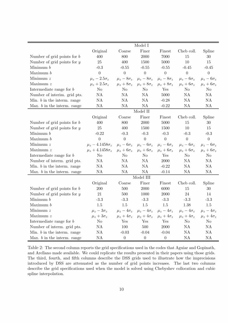
Table 2 reports the grid specifications used in this paper. In order to compare the performance

of different numerical methods, we report results obtained using various DSS grid specifications,

one grid for Chebyshev collocation, and one grid for cubic spline interpolation. In Section 5.7 we

show that the results obtained using Chebyshev collocation and spline interpolation are robust

to using more grid points.

We either use evenly spaced DSS grids (as most default studies do) or we concentrate evenly

spaced asset points in an intermediate range of the DSS grids, as noted in Table 2. We also use

evenly spaced grids when we solve the model with cubic spline interpolation.

When solving Model III with interpolation methods, we use two grids for endowments, each

with the same number of points. We use one grid for endowments lower than λ, and one for

endowments higher than λ. Note that the derivative of the output cost of defaulting with

respect to output presents a discontinuity at y = λ (see equation 5). Consequently, the function

V1 displays a kink at y = λ.

Aguiar and Gopinath (2006) and Arellano (2008) do not report the exact DSS grid specifica-

tions they use, but we are able to infer that information from their codes. The second column

of Table 2 presents the grids we use to replicate their results. We refer to these grids as the

“original” grids.

5 Results

We first document how computation time can be decreased by using a one-loop algorithm that

iterates simultaneously on the value and bond price functions. Then, we present simulation

results and computation times obtained using the grids introduced in Table 2 (and one-loop

algorithms). We show that the results we obtain using Chebyshev collocation are consistent

with the results we obtain using cubic spline interpolation and that our DSS results converge

toward our interpolation results as we increase the number of grid points and the width of the

endowment grid. We later discuss inaccuracies introduced by inappropriate DSS grids. We also

discuss the inefficiency of DSS compared with interpolation methods. At the end of the section,

we show that our results with interpolation methods appear to be robust to increases in the

9

Model I

Original Coarse Finer Finest Cheb coll. Spline

Number of grid points for b 400 800 2000 7000 15 30

Number of grid points for y 25 400 1500 5000 10 15

Minimum b -0.3 -0.55 -0.55 -0.55 -0.45 -0.45

Maximum b 0 0 0 0 0 0

Minimum z µz − 2.5σz µz − 8σz µz − 8σz µz − 8σz µz − 6σz µz − 6σz

Maximum z µz + 2.5σz µz + 8σz µz + 8σz µz + 8σz µz + 6σz µz + 6σz

Intermediate range for b No No No Yes No No

Number of interim. grid pts. NA NA NA 5000 NA NA

Min. b in the interm. range NA NA NA -0.28 NA NA

Max. b in the interm. range NA NA NA -0.22 NA NA

Model II




Minimum b -0.22 -0.3 -0.3 -0.3 -0.3 -0.3

Maximum b 0 0 0 0 0 0

Minimum z µz − 4.1458σz µz − 6σz µz − 6σz µz − 6σz µz − 6σz µz − 6σz

Maximum z µz + 4.1458σz µz + 6σz µz + 6σz µz + 6σz µz + 6σz µz + 6σz

Intermediate range for b No No No Yes No No

Number of interm. grid pts. NA NA NA 2000 NA NA

Min. b in the interm. range NA NA NA -0.22 NA NA

Max. b in the interm. range NA NA NA -0.14 NA NA

Model III




Minimum b -3.3 -3.3 -3.3 -3.3 -3.3 -3.3

Maximum b 1.5 1.5 1.5 1.5 1.38 1.5

Minimum z µz − 3σz µz − 4σz µz − 4σz µz − 4σz µz − 4σz µz − 4σz

Maximum z µz + 3σz µz + 4σz µz + 4σz µz + 4σz µz + 4σz µz + 4σz

Intermediate range for b No Yes Yes Yes No No

Number of interm. grid pts. NA 100 500 2000 NA NA

Min. b in the interm. range NA -0.03 -0.04 -0.04 NA NA

Max. b in the interm. range NA 0 0 0 NA NA

Table 2: The second column reports the grid specifications used in the codes that Aguiar and Gopinath,and Arellano made available. We could replicate the results presented in their papers using those grids.The third, fourth, and fifth columns describe the DSS grids used to illustrate how the imprecisionsintroduced by DSS are attenuated as the number of grid points increases. The last two columnsdescribe the grid specifications used when the model is solved using Chebyshev collocation and cubicspline interpolation.

10

number of grid points and we conduct the test proposed by den Haan and Marcet (1994) for

evaluating the accuracy of numerical solutions.

5.1 One-loop and two-loop algorithms

In most default studies, models are solved using DSS and two loops: the outside loop iterates on

the bond price function and the inside loop iterates on the value functions. Once convergence

is attained in the value functions, the bond price function is updated using the optimal default

decisions implied by the value functions.

We find that the computation time can be decreased significantly by using a one-loop al-

gorithm that iterates simultaneously on the value and the bond price functions. For example,

using DSS with our original grids for Model III, the one-loop algorithm takes 31 seconds and the

two-loop algorithm takes 182 seconds to converge.5 The computation time per value function

iteration is smaller with the two-loop algorithm (0.11 seconds vs. 0.13 seconds) because the bond

price function is not updated in every iteration of the value function. But the number of itera-

tions of the value function required by the two-loop algorithm to converge is significantly higher.

The difference in computation time between the two algorithms would become more significant

if we wanted to use the simulated method of moments to calibrate the model, as many default

studies do.

In the remainder of the paper, we only use solutions obtained with one-loop algorithms. This

computation strategy, along with using the solution of the last period of the finite horizon version

of the model as an initial guess, implies that the algorithm approximates the equilibrium as the

limit of the equilibrium of the finite-horizon economy. We only deviate from this approach when

we use the finest grid specifications described in Table 2. In those cases, we use as the initial

guess the value functions found using the finer grids presented in the fourth column of Table 2.

(We use linear interpolation to evaluate these functions at points that do not lie on the grid.)

5We also compare the DSS computation time required by Aguiar’s and Gopinath’s (2006) Matlab code withthe computation time required by our one-loop Fortran code, using the original grids. With only transitoryshocks, their code takes 16 minutes and 58 seconds to converge and our code takes 2 minutes and 8 seconds.With only trend shocks, their code takes 7 minutes and 44 seconds to converge and our code takes 1 minute and13 seconds.

11

5.2 Simulations

Table 3 reports business cycle statistics obtained in the simulations and the computation time for

each exercise. The logarithm of income and consumption are denoted by y and c, respectively.

The trade balance (output minus consumption, TB) is expressed as a fraction of income (Y ), and

the interest rate spread (margin of extra yield over the risk-free rate, Rs) is expressed in annual

terms. Standard deviations are denoted by σ and are reported in percentage terms; correlations

are denoted by ρ.

The statistics for Models I and II were computed following Aguiar and Gopinath (2006). We

use 500 simulation samples of 1,500 periods each.6 In order to eliminate the effect of initial

conditions, we use only the last 500 periods of each sample to compute the moments reported

in the table. We detrended each variable using the Hodrick-Prescott filter with a smoothing

parameter of 1,600 and then computed standard deviations and correlations using the detrended

series. Statistics reported in Table 3 correspond to the average value of each moment across 500

samples of 500 periods.

Similarly, the moments for Model III were computed following Arellano (2008). We simulate

the model and extract samples that satisfied the following criteria: i) a default is declared

immediately after the end of the sample, ii) the sample contains 74 periods, and iii) the last

exclusion period was observed at least two periods before the beginning of the sample. Statistics

reported in Table 3 correspond to the average value of each moment across 2,000 samples of 74

periods (Arellano 2008 uses only 100 samples).

Table 3 shows that the results we obtain using Chebyshev collocation are consistent with the

results we obtain using cubic spline interpolation. In addition, Table 3 shows that the results

obtained using DSS converge to the ones we obtain using interpolation methods when the model

is solved using DSS with (i) wider endowment grids, (ii) more endowment grid points, and (iii)

more asset grid points. We explain next how each of these modifications to DSS grids helps

mitigate approximation errors.

6Aguiar and Gopinath (2006) used samples of 10,000 periods, but we do not observe any difference in resultswhen we use samples of 1,500 periods.

12

Model I


σ(y) 4.33 4.35 4.35 4.35 4.34 4.35

σ(c) 4.39 4.49 4.49 4.48 4.47 4.48

σ (TB/Y ) 0.23 0.50 0.49 0.48 0.49 0.49

σ (Rs) 0.05 0.08 0.04 0.02 0.01 0.01

ρ (c, y) 0.99 0.99 0.99 0.99 0.99 0.99

ρ (TB/Y, y) -0.37 -0.31 -0.31 -0.31 -0.30 -0.31

ρ (Rs, y) 0.56 -0.09 -0.17 -0.42 -0.61 -0.59

ρ (Rs, TB/Y ) -0.28 0.06 0.20 0.51 0.69 0.70

Defaults per 10,000 quarters 3 7 8 8 8 8

Mean debt output ratio (%) 27 25 25 25 25 25

Time to converge 2’:8” 53’:43” 27 hours 55’ 323 hours 38’:23” 13’:11”

Time per iteration 1.17” 27” 11’: 23” 8 hours 31’ 11” 5”

Model II


σ(y) 4.46 4.43 4.43 4.43 4.43 4.43

σ(c) 4.72 4.68 4.68 4.68 4.68 4.68

σ (TB/Y ) 0.98 0.94 0.94 0.94 0.95 0.94

σ (Rs) 0.33 0.15 0.08 0.07 0.07 0.07

ρ (c, y) 0.98 0.98 0.98 0.98 0.98 0.98

ρ (TB/Y, y) -0.18 -0.18 -0.18 -0.18 -0.18 -0.18

ρ (Rs, y) 0.02 0.05 0.09 0.08 0.09 0.09

ρ (Rs, TB/Y ) 0.04 0.15 0.34 0.46 0.52 0.52



Time to converge 1’:13” 46’:7” 19 hours 26’ 45 hours 4’ 28’:58” 19’:42”

Time per iteration 0.94” 33” 13’ 69’ 15” 10”

Model III


σ(y) 5.81 5.62 5.61 5.62 5.63 5.63

σ(c) 6.31 6.00 5.99 6.00 6.00 6.00

σ (TB/Y ) 1.38 1.10 1.09 1.09 1.08 1.08

σ (Rs) 6.20 2.91 2.75 2.73 2.71 2.70

ρ (c, y) 0.97 0.98 0.98 0.98 0.98 0.98

ρ (TB/Y, y) -0.23 -0.24 -0.24 -0.24 -0.23 -0.23

ρ (Rs, y) -0.20 -0.44 -0.46 -0.47 -0.48 -0.48

ρ (Rs, TB/Y ) 0.41 0.77 0.83 0.84 0.84 0.83

E(Rs) 3.78 3.40 3.40 3.39 3.37 3.34



Time to converge 31” 68’:5” 29 hours 1’ 21 hours 35’ 2 hours 29’: 58”

Time per iteration 0.13” 17” 7’:20” 1 hour 57’ 30” 9”

Table 3: Simulation results and computation time for different DSS grids and interpolation methods.

13

5.3 The width of the endowment grid

Figure 1 shows that the width of the endowment grid may affect the computation of the gov-

ernment’s borrowing decision. We chose Model I to construct Figure 1 because this is the

parameterization for which we found the highest sensitivity of the results to an increase in the

width of the endowment grid. We use the original grid specification described in the second

column of Table 2 as the starting point, and as we increase the width of the endowment grid

we also increase the number of grid points so that the distance between endowment grid points

remain constant. This allows us to control for distortions generated by using coarse grids. All

functions were constructed using the original grid for asset positions.

0.85 0.9 0.95 1 1.05 1.1 1.15 1.2

−0.285

−0.28

−0.275

−0.27

−0.265

−0.26

−0.255

−0.25

−0.245

−0.24

y

b’(

y,b

)

+−2.5 σy

+−4 σy

+−6 σy

+−8 σy

Figure 1: Optimal savings as a function of income for DSS endowment grids of different width, forModel I, and for an initial debt level of 0.252 (the average debt observed in the simulations with thefinest grid specification).

Wider endowment grids enable the DSS algorithm to compute the true default probabilities

and, therefore, the government’s true borrowing decision. For any borrowing level, the govern-

ment will choose to default in the next period if the endowment falls below some threshold.

A DSS algorithm with a narrow endowment grid would impute a zero default probability on

borrowing levels such that the lowest value in the endowment grid is above those thresholds.

14

This would introduce a downward bias in the default probability, which in turn would increase

the value of having access to capital markets, and make defaults more costly. A higher cost

of defaulting helps in sustaining higher borrowing levels in equilibrium. This may explain the

higher borrowing levels for narrower endowment grids presented in Figure 1.

5.4 The number of endowment grid points

The discretization of income shocks may generate distortions in the behavior of the equilibrium

interest rate spread. These distortions may be mitigated by using more endowment grid points.

It is apparent from Table 3 that the dispersion of the spread computed with DSS decreases and

converges toward the one computed with interpolation as the number of points in the endowment

grid increases. To make this point clearer, Table 4 presents simulation results for Model III for

the original grid specification and for two alternative grid specifications. One specification has

the original asset grid and 10 times more grid points than the original grid for endowments.7

The other specification has the original endowment grid and 10 times more grid points than the

original grid for asset levels. Table 4 indicates that, for Model III, the main problem with the

results obtained with our original DSS grids is the insufficient number of points in the endowment

grid. Keeping the number of points in the asset grid constant, a tenfold increase in the number

of points in the endowment grid (from 21 to 211) reduces the standard deviation of the spread in

the simulations from 6.20 to 3.84. In contrast, keeping the number of points in the endowment

grid constant, a tenfold increase in the number of asset grid points (from 200 to 2000) only

reduces the standard deviation of the spread in the simulations to 4.91.

Figure 2 illustrates the source of the imprecisions caused by using coarse grids for endowment

levels when solving for Model III (similar figures could be constructed for other parameterizations

of the model). The left panel of Figure 2 describes the zero-profit bond price as a function

of the borrowing level when the endowment realization equals the unconditional mean of the

endowment process. The bond price functions computed using DSS were constructed using the

original grid for asset positions (200 points). The graph also presents the bond price function

7The choice of 211 instead of 210 points for the endowment grid is meant to force the grid to contain theunconditional mean of the endowment distribution. This is useful for computing Figure 2.

15

Method DSS DSS DSS Chebyshev Spline

Number of points for b 200 200 2000 15 30

Number of points for y 21 211 21 24 14

σ (TB/Y ) 1.38 1.11 1.37 1.08 1.08

σ (Rs) 6.20 3.84 4.91 2.71 2.70

ρ (Rs, y) -0.20 -0.32 -0.16 -0.48 -0.48

ρ (Rs, TB/Y ) 0.41 0.59 0.43 0.84 0.83

E(Rs) 3.78 3.34 3.58 3.37 3.34

Table 4: Model III simulation results.

obtained using cubic splines, which is indistinguishable from the one we obtain using Chebyshev

or DSS with fine grids. The figure shows that the discretization of the income shock introduces

discontinuities in the bond price schedule, and that these discontinuities are more pronounced

when a coarser grid for endowment levels is used. The zero-profit bond price schedule represents

the set of combinations of issuance levels and bond prices the government can choose from. The

discontinuities illustrated in Figure 2 imply that there are bond prices that are taken out from

the government’s choice set. Note that these distortions could appear even without discretizing

the set of borrowing levels the government can choose from.

−0.3 −0.25 −0.2 −0.15 −0.1 −0.05 00

0.1

0.2

0.3

0.4

0.5

0.6

0.7

0.8

0.9

1

b’/A

q(b’

,y)

−0.3 −0.25 −0.2 −0.15 −0.1 −0.05 0

# point for y = 21# point for y = 211

Spline

−0.06 −0.05 −0.04 −0.03 −0.02 −0.01 0−2.13

−2.1296

−2.1292

−2.1288

b’/A

−0.06 −0.05 −0.04 −0.03 −0.02 −0.01 0−2.128

−2.1276

−2.1272

−2.1268

# y = 21 and b/y = −0.066# y = 211 and b/y = −0.066

# y = 21 and b/y = −0.042# y = 211 and b/y = −0.042

Figure 2: The left panel illustrates the zero-profit bond price as a function of the borrowing level whenthe current endowment realization coincides with the unconditional mean of the endowment process(y = 10). The right panel illustrates the government’s objective as a function of its borrowing level.The left (right) vertical axis corresponds to the case in which b/y = −0.066 (b/y = −0.042).

16

The right panel of Figure 2 illustrates how the distortions in the bond price menu affect the

optimal saving decision. The figure presents the government’s objective function and it shows

that this function tends to be increasing with respect to the borrowing level for borrowing levels

where the bond price function is flat (i.e., for levels such that the government can increase its

borrowing without decreasing the bond price). The right panel of Figure 2 shows that this may

introduce spurious convexities in the government’s objective function and, thus, it may distort

the optimal saving levels.

5.5 The number of asset grid points

The statistics presented in Tables 3 and 4 make apparent that the results obtained using DSS

depend on the number of asset grid points and converge toward the results computed with

interpolation methods as the number of asset—and endowment—grid points increases. Figure

3 shows how the optimal savings and equilibrium bond prices obtained with DSS change as the

number of grid points for assets increases. The figure considers the equilibrium functions derived

for Model II, but the same rationale applies to Models I and III. As illustrated by the figures, for

low enough growth rates, the government defaults and is excluded from capital markets, i.e., it

borrows zero. Following Aguiar and Gopinath (2006), Figure 3 imputes the price of the risk-free

bond when the country defaults and is excluded from capital markets.

In the left panel of Figure 3, the DSS borrowing level presents steps, that is, it does not

always change when (the growth rate of) income changes. Figure 3 also shows that the steps

become smaller as the number of grid points for assets increases. In models of sovereign default,

the increase in borrowing implied by an increase in income moderates the decrease in the interest

rate implied by an increase in income. Consequently, when the discrete set of borrowing levels

available to the government precludes adjustments in the borrowing level, interest rate movements

are exacerbated. This is illustrated in the right panel of Figure 3, which illustrates the bond

prices traded in equilibrium. The graph shows how the spurious spread movements generated

by the discretization of asset levels can be mitigated by augmenting the number of points in the

DSS asset grid. Note that the right panel of Figure 3 also shows that the correlation between

17

0.9 0.95 1 1.05 1.1−0.196

−0.194

−0.192

−0.19

−0.188

−0.186

−0.184

g

b’(b

,g)

DSS 5000DSS 400

0.9 0.95 1 1.05 1.10.986

0.9865

0.987

0.9875

0.988

0.9885

0.989

0.9895

0.99

0.9905

g

q(b’

(b,g

),g)

DSS 5000DSS 400

Figure 3: Model II optimal savings and bond prices accepted in equilibrium as a function of the trendshock. The graphs were computed using DSS with 1500 endowment grid points and asset grids of 400and 5000 points. The initial asset position is assumed to be equal to -0.19.

income and spread paid in equilibrium may be contaminated with the spurious spread volatility

introduced by using DSS with coarse grids.

5.6 Computation efficiency

As expected, Table 3 shows that we can mitigate the approximation errors implied by DSS as

we increase the number of grid points. It also shows that, for the model considered in the paper,

the number of DSS grid points needed to produce accurate results is such that it makes using

DSS with an evenly spaced grid less efficient than interpolation methods.

Table 3 also illustrates how one can improve the performance of DSS by concentrating grid

points in asset levels at which the bond price is more sensitive to the borrowing level, and in

levels that are observed more often in the model simulations. To make this point clearer, Table

5 presents simulation results for Model III obtained using DSS grids with the same number of

points but with different distributions of asset points. (In order to facilitate comparisons, we

also include the results obtained using the original DSS grid and using interpolation methods.)

The fourth column of Table 5 reports results obtained allocating 100 asset grid points between

-0.03 and 0. Note that in order to attain the density of points in this intermediate range with

an evenly distributed grid, it would be necessary to use 16,000 grid points. Table 5 shows

18

Method DSS DSS DSS Chebyshev Spline

Number of points for b 200 500 500 15 30

Number of points for y 21 500 500 24 14

Distributed Evenly Evenly Non-evenly NA Evenly

σ (TB/Y ) 1.38 1.10 1.10 1.08 1.08

σ (Rs) 6.20 3.38 2.91 2.71 2.70

ρ (Rs, y) -0.20 -0.41 -0.44 -0.48 -0.48

ρ (Rs, TB/Y ) 0.41 0.67 0.77 0.84 0.83

E(Rs) 3.78 3.44 3.40 3.37 3.34

Time to converge 31” 67’:51” 68’:5” 2 hours 29’: 58”

Time per iteration 0.13” 17” 17” 30” 9”

Table 5: Model III simulation results for different allocations of DSS asset grid points.

that the computation time does not change significantly when we modify the distribution of

asset grid points, and that DSS imprecisions are mitigated by concentrating asset points in the

intermediate range. One disadvantage of using DSS with an uneven distribution of grid points

is that grids have to be tailor-made for the model’s parameterization, which would make it

more cumbersome to perform tasks such as calibrating the model using the simulated method of

moments or conducting comparative static exercises.

In addition, Table 3 illustrates that the computation time is lower with spline interpolation

than with Chebyshev collocation for the three parameterizations considered in the paper. In

fact, for Model III, the computation time with Chebyshev collocation is higher than with our

DSS coarse grids, which only produce small inaccuracies in the results. Recall that the discussion

of the imprecisions implied by DSS presented in the previous subsections indicates that these

imprecisions appear because the bond price is quite sensitive to the borrowing level. In Model

III, the bond price is less sensitive to the borrowing level and, therefore, it is less difficult to

mitigate the effect of the imprecisions implied by DSS.

5.7 Robustness of results obtained with interpolation methods

Table 6 illustrates that the results we obtain with interpolation methods reported in Table

3 are robust to increasing the number of grid points. The first (second) number in the pair

19

Model I

Cheb coll. Spline(15, 10) (30,20) (30,15) (50,30)

σ(y) 4.34 4.34 4.36 4.35σ(c) 4.47 4.47 4.48 4.48σ (TB/Y ) 0.49 0.49 0.49 0.49σ (Rs) 0.01 0.01 0.01 0.01ρ (c, y) 0.99 0.99 0.99 0.99ρ (TB/Y, y) -0.30 -0.30 -0.31 -0.31ρ (Rs, y) -0.61 -0.58 -0.59 -0.59ρ (Rs, TB/Y ) 0.69 0.70 0.70 0.70Rate of default (per 10,000 quarters) 8 8 8 8Mean debt output ratio (%) 25 25 25 25

Model II

(15, 10) (30,20) (30,15) (50,30)σ(y) 4.43 4.43 4.43 4.43σ(c) 4.69 4.68 4.68 4.68σ (TB/Y ) 0.95 0.95 0.94 0.94σ (Rs) 0.07 0.07 0.07 0.07ρ (c, y) 0.98 0.98 0.98 0.98ρ (TB/Y, y) -0.18 -0.18 -0.18 -0.18ρ (Rs, y) 0.09 0.09 0.09 0.09ρ (Rs, TB/Y ) 0.52 0.51 0.52 0.53Rate of default (per 10,000 quarters) 22 23 22 22Mean debt output ratio (%) 19 19 19 19

Model III

(15, 24) (30,34) (30,14) (50,30)σ(y) 5.63 5.62 5.63 5.63σ(c) 6.00 6.00 6.01 6.00σ (TB/Y ) 1.08 1.08 1.08 1.08σ (Rs) 2.71 2.67 2.70 2.68ρ (c, y) 0.98 0.98 0.98 0.98ρ (TB/Y, y) -0.23 -0.23 -0.24 -0.23ρ (Rs, y) -0.48 -0.49 -0.48 -0.48ρ (Rs, TB/Y ) 0.84 0.84 0.83 0.85E(Rs) 3.38 3.38 3.34 3.34Rate of default (per 10,000 quarters) 74 75 74 74Mean debt output ratio (%) 4 4 4 4

Table 6: Simulation results using different grid configurations for Chebyshev collocation and splineinterpolation.

20

characterizing a column is the number of points in the asset (endowment) grid.

5.8 A test of the accuracy of the numerical solutions

In this subsection we conduct the test proposed by den Haan and Marcet (1994) for evaluating

the accuracy of numerical solutions. We conduct the test for each of the numerical solutions

analyzed in this paper and summarized in Table 3. The test evaluates whether the Euler equation

is satisfied in the simulations and is implemented using 5,000 samples of 1,500 periods each. We

remove the first 10 periods of each sample, all periods in which the economy is excluded with the

exception of periods in which a default is declared, and the first 10 periods after the end of an

exclusion spell. We did not observe significant changes in results if more periods after the end

of exclusion spells were removed from the samples.

den Haan and Marcet (1994) derive the asymptotic distribution of any weighted sum of resid-

uals of the Euler equation under the null hypothesis that the Euler equation is satisfied in the

simulations. The test consists of comparing that probability distribution with the distribution

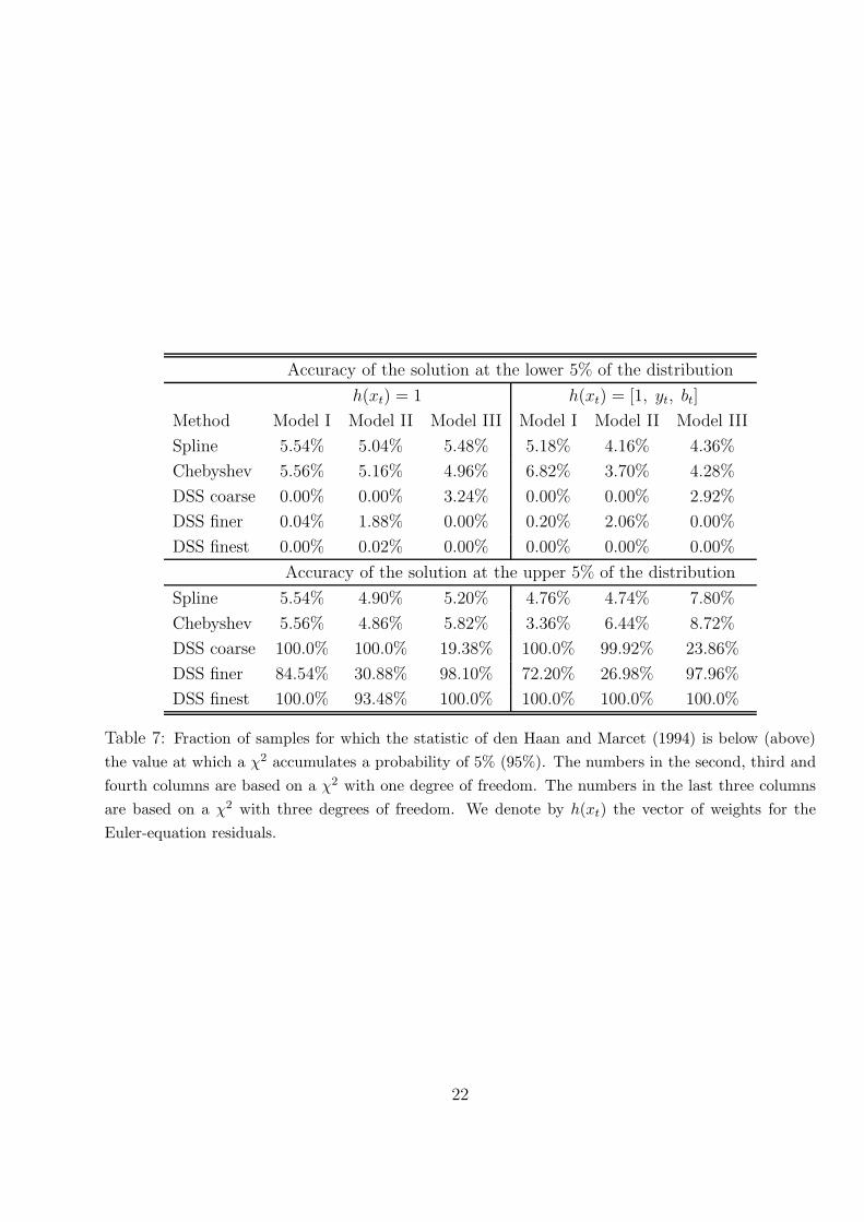
observed in the simulations. Table 7 summarizes the comparison using two statistics: the fre-

quency of samples for which the weighted sum of residuals takes values within the 5 percent

left (right) tail of the asymptotic distribution. Table 7 indicates that interpolation procedures

approximate the equilibrium with reasonable accuracy (values are close to 5 percent).8

One might also conclude from Table 7 that DSS does not approximate the solution with

reasonable accuracy. However, we found evidence suggesting that the main reason for the large

discrepancies reported in Table 7 can be traced back to approximation errors in the calculation

of the residuals of the Euler equation. One of the terms of the Euler equation depends on the

derivative of the zero-profit bond price with respect to the borrowing level (see, for example,

Hatchondo and Martinez 2009). We denote this derivative by q1. When the model is solved

using DSS, the value of q1 evaluated at the ith component of the grid for asset positions and at

the jth component of the grid for endowment shocks is approximated as

8The larger discrepancies are observed in the last column of Table 7 for the right tail of the distribution.When the Euler equation residuals in period t + 1 weighted by the vector [1, yt, bt], the correlation between theresiduals and the residuals weighted by the endowment realization in the previous period is close to 0.99. Thehigh co-linearity between these two series reduces the precision of the test.

21

Accuracy of the solution at the lower 5% of the distribution

h(xt) = 1 h(xt) = [1, yt, bt]

Method Model I Model II Model III Model I Model II Model III

Spline 5.54% 5.04% 5.48% 5.18% 4.16% 4.36%

Chebyshev 5.56% 5.16% 4.96% 6.82% 3.70% 4.28%

DSS coarse 0.00% 0.00% 3.24% 0.00% 0.00% 2.92%

DSS finer 0.04% 1.88% 0.00% 0.20% 2.06% 0.00%

DSS finest 0.00% 0.02% 0.00% 0.00% 0.00% 0.00%

Accuracy of the solution at the upper 5% of the distribution

Spline 5.54% 4.90% 5.20% 4.76% 4.74% 7.80%

Chebyshev 5.56% 4.86% 5.82% 3.36% 6.44% 8.72%

DSS coarse 100.0% 100.0% 19.38% 100.0% 99.92% 23.86%

DSS finer 84.54% 30.88% 98.10% 72.20% 26.98% 97.96%

DSS finest 100.0% 93.48% 100.0% 100.0% 100.0% 100.0%

Table 7: Fraction of samples for which the statistic of den Haan and Marcet (1994) is below (above)

the value at which a χ2 accumulates a probability of 5% (95%). The numbers in the second, third and

fourth columns are based on a χ2 with one degree of freedom. The numbers in the last three columns

are based on a χ2 with three degrees of freedom. We denote by h(xt) the vector of weights for the

Euler-equation residuals.

22

q1(bi, yj) =q (bi+∆, yj) − q (bi−∆, yj)

bi+∆ − bi−∆

, (6)

with ∆ = 1. We find that the sample distribution of the Den Haan and Marcet’s statistic is quite

sensitive to the value of ∆ used to approximate q1. Furthermore, the value of ∆ that generates

the best results for the test depends on the model parameterization and grid configuration. The

approximation of q1 is highly sensitive to the value of ∆ because, as illustrated by Figure 2,

typically the zero-profit bond price obtained with DSS presents steps. As the number of asset

grid points increases, the steps become narrower but more frequent, so the local approximation

of q1 does not necessarily become more accurate. We find that, even for our finest DSS grids

(for which we obtained results very similar to those obtained with interpolation methods), the

bond-price derivative is quite sensitive to the choice of ∆. Overall, we cannot conclude that the

poor performance of the DSS solutions according to Den Haan and Marcet’s test is due to the

lack of accuracy in the approximation of the equilibrium.

6 Robustness of findings in Aguiar and Gopinath (2006)

and Arellano (2008)

This section discusses inaccuracies in the results presented by Aguiar and Gopinath (2006) and

Arellano (2008). In order to do so, we compare key statistics from the simulations presented

in those papers with the same statistics computed using spline interpolation and Chebyshev

collocation (the latter are similar to statistics obtained using DSS with fine grids).9

The second and fifth columns of Table 8 present the statistics reported by Aguiar and

Gopinath (2006) in Table 3 of their paper (page 77). The remaining columns present the same

statistics computed using spline interpolation and Chebyshev collocation. Table 8 indicates that

9Note that the results reported in Table 3 for the original grids resemble the ones reported in Aguiar andGopinath (2006) and Arellano (2008). The largest differences between our results with the original grids andtheirs appear in Model III. This is explained by a bug in the code used by Arellano (2008), where the post-defaultvalue function is computed without considering the possibility that the sovereign may regain access to capitalmarkets in the next period. Once the value function is computed correctly, the default rate and mean spreadincrease while the debt-to-output ratio decreases.

23

Model I Model II

AG Spline Chebyshev AG Spline Chebyshev

σ(y) 4.32 4.35 4.34 4.45 4.43 4.43

σ(c) 4.37 4.48 4.47 4.71 4.68 4.69

σ (TB/Y ) 0.17 0.49 0.49 0.95 0.94 0.95

σ (Rs) 0.04 0.01 0.01 0.32 0.07 0.07

ρ (c, y) 0.99 0.99 0.99 0.98 0.98 0.98

ρ (TB/Y, y) -0.33 -0.31 -0.30 -0.19 -0.18 -0.18

ρ (Rs, y) 0.51 -0.59 -0.61 -0.03 0.09 0.09

ρ (Rs, TB/Y ) -0.21 0.70 0.69 0.11 0.52 0.52



Maximum Rs (basis point) 23 29 30 151 97 97

Table 8: Simulation results in Aguiar and Gopinath (2006) and with spline interpolation and Chebyshev

collocation.

the co-movement between the spread and income reported by Aguiar and Gopinath (2006) is

affected by inaccuracies introduced by inappropriate DSS grids. We find that the correlation

between spread and income is -0.6 in Model I (with shocks to the income level) and 0.1 in Model

II (with shocks to the growth rate of income). In contrast, Aguiar and Gopinath (2006) report

that this correlation is 0.5 in Model I and -0.03 in Model II. Thus, our results cast doubt on their

claim that with Model II, “Some improvements over Model I are immediately apparent. Both

the current account and interest rates are countercyclical and positively correlated.... ” (page 79

in Aguiar and Gopinath 2006). Our findings imply that the ability of the model to fit the data

does not necessarily improve when one assumes an income process with shocks to the growth

rate instead of a standard process with shocks to the level.

At the top of Table 9, we present the statistics reported in Table 4 (page 706) of Arellano

(2008). The table also presents the same statistics computed using spline interpolation and

Chebyshev collocation. Table 9 indicates that more than half of the spread volatility reported in

Arellano (2008) is accounted for by inaccuracies introduced by inappropriate DSS grids. Figure

4 further illustrates the effects of these inaccuracies. The figure replicates the counterfactual

exercise presented in Arellano (2008) on page 707. We feed Model III with the time series of

the Argentine GDP between 1993 and 2001, and then compute the spread behavior predicted

24

Arellano (2008)

Default episodes σ(x) ρ(x, y) ρ(x, Rs)

Interest rate spread 24.32 6.36 -0.29

Trade balance -0.01 1.50 -0.25 0.43

Consumption -9.47 6.38 0.97 -0.36

Output -9.60 5.81 -0.29

Other statistics

Mean debt (percent output) 5.95 Mean Spread 3.58

Default probability 3.00 Output deviation in default -8.13

Spline



Trade balance -0.72 1.08 -0.23 0.83

Consumption -9.39 6.00 0.98 -0.59

Output -9.48 5.63 -0.48

Other statistics



Chebyshev



Trade balance -0.72 1.08 -0.23 0.84

Consumption -9.42 6.00 0.98 -0.60

Output -9.50 5.63 -0.48

Other statistics



Table 9: Simulation results in Arellano (2008) and with spline interpolation and Chebyshev collocation.

by the model. The behavior we compute using the original grids resembles the one computed by

Arellano (2008), which displays a significantly higher spread prior to the default episode of 2001

than in the 1995 Tequila crisis. This is inconsistent with the spread behavior obtained using

interpolation methods or DSS with our finest grid specification. Figure 4 also shows that the

implied spread behavior obtained using DSS with the finest grid is indistinguishable from the

behavior obtained using interpolation methods.

The imprecisions described in Table 9 and Figure 4 are caused by imprecisions in the ap-

proximations of the optimal policies. This is illustrated in Figure 5, which replicates the optimal

saving rule and equilibrium interest rates described by Figures 3 and 4 in Arellano (2008) (pages

25

93 Q2 95 Q2 97 Q2 99 Q2 01 Q20

0.05

0.1

0.15

0.2

0.25

0.3

0.35

Spr

ead

ChebychevSplineDSS 200/21DSS 6000/200

Figure 4: Implied spread behavior when the endowment realization coincides with the time series ofArgentine GDP between 1993 and 2001.

704 and 705). Figure 5 shows that the optimal saving policies and equilibrium interest rates

obtained with interpolation methods or with DSS and a sufficiently dense grid specification are

significantly different from the optimal saving rule and equilibrium interest rates obtained using

the original grids.

7 Conclusions

We show that the use of DSS with inappropriate grid specifications introduces approximation

errors that contaminate the results presented by Aguiar and Gopinath (2006) and Arellano

(2008). These imprecisions led Aguiar and Gopinath (2006) to conclude that income processes

with shocks to the growth rate help models of sovereign default generate a countercyclical interest

rate and, thus, help the baseline default model generate the positive correlation between the

interest rate and the current account observed in the data. Besides, more than half of the

spread volatility reported by Aguiar and Gopinath (2006) and Arellano (2008) results from

approximation errors.

We also find that interpolation methods may be significantly more efficient than DSS for

26

−0.25 −0.2 −0.15 −0.1 −0.05 0 0.05 0.1 0.15−0.12

−0.1

−0.08

−0.06

−0.04

−0.02

0

0.02

0.04

0.06

0.08

b/A

b’(b

,y)/

A

y low

y high

DSS 6000/2000DSS 200/21 & y lowDSS 200/21 & y highChebychevSpline

−0.08 −0.06 −0.04 −0.02 0 0.020.06

0.08

0.1

0.12

0.14

0.16

0.18

0.2

b/A

Inte

rest

Rat

e

y low

y high

DSS 6000/2000DSS 200/21 & y lowDSS 200/21 & y highChebychevSpline

Figure 5: Model III optimal savings and implied interest rate as functions of the initial asset positionfor y = 0.93 (y low) and y = 1.02 (y high).

solving default models and that the inefficiency of DSS is more severe for parameterizations

that feature a high sensitivity of the bond price to the borrowing level for the borrowing levels

observed more often in the simulations. As in Aguiar and Gopinath (2006) and Arellano (2008),

the models studied in the growing literature on sovereign default are usually solved using DSS

with evenly spaced grid points and algorithms that use two loops. We show that the efficiency of

DSS can be greatly improved by (i) using a one-loop algorithm and (ii) concentrating grid points

in asset levels at which the bond price is more sensitive to the borrowing level, and in levels that

are observed more often in the simulations.

27

A Appendix

In this section we describe our computational strategy. For expositional simplicity, the discussion

assumes that shocks affect only the endowment level and not the growth rate of the endowment.

When solving the model using Chebyshev collocation, the value functions V0 and V1 are

approximated as a weighted sum of Chebyshev polynomials for all (b, y) ∈ [b b] × [y y]. When

b or y takes values outside the set [b b] × [y y], the value functions are approximated using a

first-order Taylor approximation evaluated at the closest point in the set [b b] × [y y].

When solving the model using cubic spline interpolation, we first define evenly distributed

grids of asset positions and endowment shocks. Those grid vectors and the matrices of values

for V0 and V1 are used to compute the breakpoints and coefficients for the piecewise cubic

representation using the routine CSDEC from the IMSL library. The routine is based on de Boor

(1977), chapter 4. More precisely, when evaluating V0 at a point (b, y) in the set [b b]× [y y], we

first interpolate over asset positions and compute the vector(

V0(b, y1), ...V0(b, yNy))

, where Ny

denotes the number of grid points for endowment shocks. Then, we interpolate over endowment

positions to compute V0(b, y). As with Chebyshev collocation, when the asset position or the

endowment shock takes values outside the minimum or maximum grid values, we evaluate the

value functions using a first-order Taylor approximation. We use the not-a-knot condition to

determine the value of the derivatives at the end points.

The algorithm used to solve for the equilibrium with interpolation methods works as follows.

First, we specify initial guesses for V0 and V1. We use as initial guesses the continuation values

at the last period of the finite-horizon version of the model, i.e., for values of (bi, yj) on the grid

for asset levels and endowment shocks,

V(0)0 (bi, yj) = u (yj + bi) and

V(0)1 (yj) = u (yj − φ(yj)) .

Second, we solve the optimization problem defined in equations (2)-(4) for each point on

the grid of assets and endowment shocks. In order to solve for the optimum, we first find a

28

candidate value for the optimal borrowing level using a global search procedure. That candidate

value is then used as an initial guess in the optimization routine UVMIF from the IMSL library.

That routine uses a quasi-Newton method to find the maximum value of a function. Each time

the borrower’s objective function is evaluated, it computes the expectation E (V (b′, y′ | y)) using

Gauss-Legendre quadrature points and weights, and using V(0)0 and V

(0)1 to approximate for the

next-period continuation values. The bond price function q(b, y) is evaluated using the optimal

default decision derived from V(0)0 and V

(0)1 . The solution found at each point on the grid for

asset and endowment shocks is then used to compute the new continuation values V(1)0 and V

(1)1 .

Third, we evaluate whether the maximum absolute deviation between the new and previous

continuation values is below 10−6. If it is, a solution has been found. If it is not, we repeat the

optimization exercise using the new continuation values V(1)0 and V

(1)1 to compute the expected

value function at each grid point for assets and endowments and to evaluate the bond price

function q(b, y) faced by the borrower. We repeat the procedure until the maximum absolute

deviation between the new and previous continuation values is below 10−6.

Note that the algorithm only imposes differentiability on V0 and V1.10 The algorithm may

very well capture discontinuities in the optimal saving rule (as illustrated in Figure 5) or kinks

in the bond price function (as illustrated in Figure 2).

10For that reason, when solving Model III, we partition the grid for endowment shocks. The output costassumed in Arellano (2008) displays a kink at y = λ, which generates a kink in the function V1.

29

References

Aguiar, M. and Gopinath, G. (2006). ‘Defaultable debt, interest rates and the current account’.

Journal of International Economics, volume 69, 64–83.

Aguiar, M. and Gopinath, G. (2007). ‘Emerging markets business cycles: the cycle is the trend’.

Journal of Political Economy , volume 115, no. 1, 69–102.

Arellano, C. (2008). ‘Default Risk and Income Fluctuations in Emerging Economies’. American

Economic Review , volume 98(3), 690–712.

Athreya, K. (2002). ‘Welfare Implications of the Bankruptcy Reform Act of 1999’. Journal of

Monetary Economics, volume 49, 1567–1595.

Benjamin, D. and Meza, F. (2009). ‘Total Factor Productivity and Labor Reallocation: The

Case of the Korean 1997 Crisis’. The B.E. Journal of Macroeconomics (Advances), volume 9,

Article 31.

Chatterjee, S., Corbae, D., Nakajima, M., and Rıos-Rull, J.-V. (2007). ‘A Quantitative Theory

of Unsecured Consumer Credit with Risk of Default’. Econometrica, volume 75, 1525–1589.

Cuadra, G., Sanchez, J. M., and Sapriza, H. (forthcoming). ‘Fiscal policy and default risk in

emerging markets’. Review of Economic Dynamics .

Cuadra, G. and Sapriza, H. (2008). ‘Sovereign default, interest rates and political uncertainty in

emerging markets’. Journal of International Economics, volume 76, 78–88.

de Boor, C. (1977). A Practical Guide to Splines. Springer-Verlag.

den Haan, W. J. and Marcet, A. (1994). ‘Accuracy in simulations’. Review of Economic Studies ,

volume 61, 3–17.

Eaton, J. and Gersovitz, M. (1981). ‘Debt with potential repudiation: theoretical and empirical

analysis’. Review of Economic Studies , volume 48, 289–309.

30

Hatchondo, J. C. and Martinez, L. (2009). ‘Long-duration bonds and sovereign defaults’. Journal

of International Economics, volume 79, 117–125.

Hatchondo, J. C., Martinez, L., and Sapriza, H. (2007). ‘Quantitative Models of Sovereign

Default and the Threat of Financial Exclusion’. Economic Quarterly , volume 93, 251–286.

No. 3.

Hatchondo, J. C., Martinez, L., and Sapriza, H. (2009). ‘Heterogeneous borrowers in quantitative

models of sovereign default.’ International Economic Review . Forthcoming.

Li, W. and Sarte, P.-D. (2006). ‘U.S. consumer bankruptcy choice: The importance of general

equilibrium effects’. Journal of Monetary Economics, volume 53, 613–631.

Livshits, I., MacGee, J., and Tertilt, M. (2008). ‘Consumer Bankruptcy: A Fresh Start’. Amer-

ican Economic Review , volume 97, 402–418.

Neumeyer, P. and Perri, F. (2005). ‘Business cycles in emerging economies: the role of interest

rates’. Journal of Monetary Economics, volume 52, 345–380.

Schmitt-Grohe, S. and Uribe, M. (2003). ‘Closing small open economy models’. Journal of

International Economics, volume 61, 163–185.

Uribe, M. and Yue, V. (2006). ‘Country spreads and emerging countries: Who drives whom?’

Journal of International Economics, volume 69, 6–36.

31

Quantitative properties of sovereign default models: Solution methods matter

Documents

Transcript of Quantitative properties of sovereign default models: Solution methods matter