1

The Dynamics of Sovereign Credit Default Swap and Bond Markets:

Empirical Evidence from the 2001-2007 Period*

Erdem Aktug Doctoral Candidate College of Business

& Economics Lehigh University

rea204@lehigh.edu (610) 758-5930

Geraldo Vasconcellos Professor of Finance College of Business

& Economics Lehigh University gmv0@lehigh.edu (610) 758-3440

Youngsoo Bae Assistant Professor of Economics

College of Business & Economics

Lehigh University yob206@lehigh.edu

(610) 758-5342

Abstract

This paper evaluates the dynamic relationship between sovereign credit default swap (CDS) and bond markets for the 2001-2007 period. We compare monthly five year CDS premiums with Emerging Market Bond Index Global (EMBIG) stripped spreads for thirty sovereign bonds, providing a thorough analysis of sovereign credit markets with an extensive and high quality data set. Our first finding is that the relationship between sovereign CDS and bond markets has strengthened over time. Second, we show bond markets’ leading role in the price discovery mechanism. This result is in sharp contrast with studies on corporate credit markets and it reveals the inefficiencies surrounding sovereign credit markets. Third, we provide an econometric methodology which is more meaningful in the sovereign context. Consequently, we propose a new measure to check for the appropriate error correction mechanism in the Vector Error Correction Model (VECM) framework. The results of our study possess valuable information for issuers, regulators, investors, and traders of sovereign securities.

This draft: October 20th, 2008. Comments welcomed.

Please do not quote without permission of the authors. * This paper is an outgrowth of the doctoral dissertation work of the first author at Lehigh University. We are grateful to the other members of the dissertation committee, Nandu (Nandkumar) Nayar, Vladimir Dobric, and Parveen Gupta for providing their input. Special thanks to JPMorgan and Markit Group for providing the data.

2

1 - Introduction Credit Default Swap (CDS) markets give bond holders the opportunity to hedge their risks. An investor who owns a sovereign bond can eliminate his risk by buying the corresponding CDS. A hedge fund manager can make arbitrage profits if buying the bond and the CDS of the same sovereign gives a higher rate of return compared to her cost of borrowing. Similarly, a speculator who predicts that a sovereign will be in distress in the near future can bet on the increase on CDS prices. Or, more commonly, an issuing entity such as a bank can take advantage of the asymmetric information in the sovereign markets and make mark-up profits from the insurance business (Andritzky, 2005). Recently, it has also become a common practice for rating agencies to adopt various new marked-to-market risk indicators, such as CDS Implied Ratings, revealing the significance of CDS markets. Sovereign bonds are the securities issued by sovereign governments. Sovereign CDSs, however, are insurance policies provided by a third financial party, such as a bank or a hedge fund, against the risk of default by a sovereign. The protection seller has to deliver the reference bond at its par value when a credit event occurs. In return, the protection buyer makes periodic payments to the seller until the maturity date of the CDS contract or until a credit event occurs. The periodic payment, which is usually expressed as a percentage (in basis points) of the principal, is called the CDS premium (Zhu, 2006). The CDS markets also serve as a financial tool for investors and traders to short the sovereign bonds without any liquidity problem (Blanco et al., 2005). The major players (buyers and sellers) in the CDS markets are, in order of importance, banks, insurance companies, security houses, and hedge funds (Chan-Lau and Kim, 2004). A sovereign bond spread is a premium paid by the issuing government to compensate for the additional risk. This premium is generally calculated as the difference between the yield of the risky sovereign bond and the yield of a risk-free bond, such as a US or German government bond, or a risk-free market rate such as a LIBOR or Swap Rate. Unlike the bond spreads, the CDS premiums (or spreads) do not incorporate any risk-free benchmarks into their calculations. However, this premium is determined by the issuing entity with a careful eye on the sovereign bond markets, therefore there is a very close relationship between the sovereign bond spreads and the sovereign CDS premiums. In efficient markets (such as the US corporate bond markets), arbitrage forces CDS spreads to be approximately equal to the underlying bond spreads in the absence of market friction, therefore driving the basis, the difference between the CDS and the corresponding bond spread, to zero in the long-run (Hull-White, 2000 and Zhu, 2006). Starting in the mid 1990s, the international bond markets gained more importance. During this time period, international financial crises and subsequent restructurings led to better functioning markets for sovereign debt. In terms of sovereign CDS markets, however, it is hard to come to any conclusions since these markets are in their infancy. Therefore, the interaction between sovereign CDS and bond markets stands as a promising research area. Uncovering the recent development or irregularities in the sovereign credit markets will help governments, investors, and various regulators improve the transparency of these markets.

3

In modern finance literature, there are numerous studies focusing on the relationship between bond and CDS spreads. One group of the studies emphasizes the relationship between bond spreads, CDS spreads, stock prices or stock market indices, and the ratings assigned by major agencies such as S&P, Moody’s, and Fitch. Most of these studies focus on the corporate bond markets as opposed to sovereigns, since the data availability for the latter is very limited. Another group of authors focus on the local (macroeconomic) and global factors affecting the spreads. Specifically, this group tries to explain the sovereign CDS and bond spreads with more frequent data such as daily equity indices, daily volatility measures, exchange rates, and interest rates. A third line of research deals with the pricing issues in sovereign CDS markets. This line of investigation studies terms such as recovery value, loss rate, and credit event intensities. For instance, Andritzky (2005) reveals that the recovery values are higher than traditional assumptions (25%) in general CDS pricing models. Thus we observe over-pricing in Sovereign CDS Markets in recent distress periods. In addition, Pan and Singleton (2005) assert that the term structure of sovereign bonds and CDSs convey important signals about the implied default probabilities and recovery rates. A more detailed summary about the literature on sovereign CDS and bond markets can be found in Appendix 1. In this paper, we evaluate the dynamics of sovereign credit default swap (CDS) and bond markets for the 2001-2007 period. The main contribution of our study is to provide a thorough analysis of the sovereign credit markets with an extensive and high quality data set. Our results can be summarized as follows. First, we find that sovereign CDS and bond markets have become more integrated over time. However, these markets are still less efficient than the corporate bond markets. This is mainly the result of the sovereign bond markets’ leading role in price discovery mechanism. Next, we provide an econometric methodology which is more meaningful in the sovereign context. Additionally, we provide a new measure to check for the appropriate error correction mechanism in the Vector Error Correction Model (VECM) framework. The results of our study possess valuable information for regulators, investors, and traders of sovereign securities. For instance, our results might help to alert international authorities about the impending problems in sovereign markets. Accordingly, this might bring additional assistance to those sovereigns in aligning the bond markets with the CDS markets. Additionally, as Andritzky (2005) points out, banks and arbitrageurs might face more restrictions in the mark-up pricing for insurance or trading activities which might bring instability to these economies. Since the CDS spreads are marked-to-market signals for country risk, any speculation in these markets might cause significant harm to the emerging economies as a whole. Lastly, our study also points to some arbitrage opportunities for traders and hedge-funds which have an interest in sovereign securities. Our paper proceeds as follows. First, we provide a brief literature review on the relationship between the sovereign CDS and bond markets. Next, we state our hypotheses and explain how we contribute to existing literature. Third, we describe our data set in detail and go over some definitions. Fourth, we lay out the econometric methodology and perform empirical time series analysis. In this step we also provide comprehensive tables to summarize the majority of our findings. In the final step, we wrap up the whole discussion, and relate the findings to the modern economic and finance theory. We also point out some of the shortcomings of our study and address some potential directions for further research in our conclusion.

4

2 - Literature Review

A - The Relationship between CDS & Bond Markets First, the paper by Zhu (2006) covers daily rates from 1999 to 2002 for twenty-four (19 US, 2 Europe, 2 Asia) corporate entities. Zhu demonstrates (via cointegration test) that the long-run equilibrium relationship holds between CDS and Bond markets. In general, a long-run equilibrium is a stable and arbitrage free state in which CDS and Bond spreads converge to each other, thus the basis converges to zero. Zhu adds that short-run deviations occur due to the high responsiveness of CDS markets to changing credit conditions. Specifically, the author argues that the changes in credit and liquidity conditions are the most important factors affecting the basis. In terms of market efficiency, Zhu shows that CDS markets lead bond markets in price discovery. In a similar paper, Blanco, Brennan, and Marsh (2005) perform an empirical study for a sample of thirty-three (16 US, 17 European) investment grade firms with a time series data which covers January 2, 2001 through June 20, 2002. They find two key factors accounting for the deviation from the parity. In the long run, the imperfections in the contract specifications and measurement errors cause markets to drift away from the equilibrium. Specifically, the authors suggest cheapest-to-deliver (CTD) options, unavailability or cost of short selling (non-zero repo costs) in bond markets, and the liquidity premium as potential imperfections. In the short-run, the deviation from the parity is mainly a result of the leading role of CDS spreads in the price discovery process. Overall, the authors confirm that the cointegration relation holds in the majority of the entities, and CDS prices lead bond prices. They also note that US markets are much more efficient compared to European Markets. Third, Norden and Weber (2004) analyze a sample of fifty-eight (35 Europe, 20 US, 3 Asia) firms over the 2000-2002 period. They conclude that the change in stock prices lead the changes in CDS and bond spreads in their three dimensional vector autoregressive (VAR) model. The cointegration relation is shown to hold in the majority of the entities (US 15/20, Europe 20/35). In addition, the study confirms that the CDS markets lead bond markets in price discovery for the US firms, whereas bond markets contribute to price discovery for European firms. In other words, their analysis shows that the markets are more efficient for US compared to non-US entities, which is in line with the first two papers above. However, the authors also use Granger Causality test to make predictions on the CDS and bond markets. This approach casts a considerable doubt since the econometric literature asserts that the Granger Causality is not an appropriate test for cointegrated systems (Enders, 2004). Fourth, we can refer to the European Bond Market Study Annex B (ECB, 2004) as a comparable study. Data includes fifteen companies with liquid euro-dominated bonds from October 2001 to June 2004 on a daily basis. The analysis shows that for 68% of the analyzed companies, the cointegration relation is confirmed. In addition, this study also uses the Gonzalo-Granger (1995) measure for the price discovery, and concludes that for 67% of the entities, the CDS markets are leading the bond markets. The last paper we can mention related to corporate markets is by Hull, Predescu, and White (2004). Their study concludes that the CDS prices rise

5

sharply and predict all types of negative rating actions (actual downgrade, negative outlook, negative review) for a large sample of corporate bonds. Our work extends the literature concerning corporate studies towards sovereign CDS and bond markets. The only two papers which focus on the sovereign case are the IMF working paper by Chan-Lau and Kim (2004), and the Federal Reserve System Discussion Paper by Ammer and Cai (FRB, 2007). In the former paper, the authors use daily CDS spreads, daily JPMorgan’s EMBI+ spreads, and daily MSCI equity indices for eight emerging markets covering the March 2001 - May 2003 period. Specifically, they perform cointegration and causality tests, and price discovery analysis for three markets: the stock market, the bond market, and the CDS market. They conclude that there is no equilibrium relationship between Bond and CDS markets in Mexico, the Philippines, and Turkey; whereas the cointegration relation is significant for Brazil, Bulgaria, Colombia, Russia, and Venezuela. In addition, they find mixed results in terms of price discovery and causality. For instance, in Russia and Colombia, the CDS market is claimed to be the source of price discovery. For Brazil and Bulgaria, the study reveals that the bond and CDS markets are equally important in price discovery. The study also demonstrates the negligible effect of the equity markets in price discovery (except Russia). In the latter paper, Ammer and Cai (FRB, 2007) emphasize the effect of Cheapest-to-Deliver (CTD) option in sovereign CDS contracts. In addition to the 5-year CDS spreads, the authors obtain the corresponding bond spreads from Bloomberg’s fair market curve analysis. The authors also criticize the use of EMBI+ spreads for several reasons, such as the variation in maturity structure over time and across sovereign entities, and inclusion of Brady Bonds with collateral enhancements. This paper covers nine emerging markets and daily spreads from 2001 to 2005. However, the price discovery tests are only performed for seven countries and 58% of the time CDS spreads are found to lead bond spreads, which is in contrast with the IMF study by Chan-Lau and Kim. Both papers on sovereign credit markets conclude that the most liquid markets lead the others in general. Furthermore, they assert that the CTD option shows up as an important factor in market imperfections. From this point of view, it makes sense to see CDS markets leading bond markets during periods of distress, since the liquidity shifts towards CDS markets during distress periods, making them more liquid. Overall, the findings in these studies deviate from the findings of the corporate literature. These findings lead to question the efficiency of the sovereign bond markets. Compared to the studies above, our research spans a more comprehensive period and it covers a larger cross section. We extend the corporate research to sovereign cases while improving the existing literature on sovereign credit markets technically as well as conceptually. Overall, we examine sovereign CDS and bond markets from a broader and a more robust point of view.

6

B - Explaining the Spreads: Global and Local Factors Longstaff, Pan, Pederson, and Singleton (NBER, 2007) assert that sovereign risk is mainly driven by global factors (VIX Index, US corporate high yield spreads) rather than local factors (local stock market return, exchange rates, foreign reserves). The authors use monthly CDS spreads in 2000-2007 for 23 emerging markets plus 3 developed markets in their study. They find that the CDS spreads are majorly driven by three main classes of global factors: global financial markets, global risk premia, and global investment flows. The details can be found in Appendix 1. In addition, Powell and Martinez (Inter-American Development Bank, 2008) argue in the same way that a small number of global factors can explain the variation in CDS spreads. However, they do show that the growth, fiscal balance, and EU membership effect the spreads over and above the effect of the credit ratings assigned by the agencies. Their data includes daily CDS spread information for 20 emerging markets for the 2006-2007 time period. In contrast to the studies highlighted in part B, our paper focuses solely on the relationship between sovereign CDS and Bond Spreads rather than explaining the spread levels. However, it is useful to include them in our review, since some of the factors pointed out in these papers might give some helpful insights on sovereign credit markets. 3 - Hypotheses and Contributions Our study is an important bridge between the corporate and sovereign literature related to the time-series characteristics of CDS and bond markets. We extend previous research in three major aspects. First, our study spans a longer time period and covers a larger cross section that has never been examined before. Specifically, we cover 30 emerging markets (monthly observations) for the 2001-2007 period. Our findings confirm that the cointegration relation between sovereign CDS and Bond markets have become stronger, thus the sovereign credit markets have matured over time. Second, our study follows a slightly different econometric methodology compared to the earlier studies. Similar to the existing literature, we use Johansen’s Cointegration Test to find out whether there is a long-run equilibrium relationship between CDS and bond markets. As a proxy for price discovery, we adopt the adjustment coefficients of the VECM framework. These coefficients tell us the speed of adjustment of the CDS and bond spreads to deviations from the long-run equilibrium. We differ from the existing literature in that we question the validity of Gonzalo-Granger (1995) scaling for price discovery in our case. Alternatively, we suggest a more meaningful and simple measure for the appropriate error correction mechanism. Third, we bring up an important discussion related to lag-length selection procedures. Our sensitivity analysis demonstrates the departure in results when we use different measures for lag-length selection. Overall, our results strengthen some of the previous findings while contradicting others. In terms of price discovery, we find that bond markets lead CDS markets, which is in line with the IMF study (Chan-Lau &

7

Kim, 2004) but in contrast with most of the corporate literature. However, we show that the equilibrium relationship between the CDS and Bond markets are more significant compared to earlier periods (Table-1). In terms of econometric methodology, we test the following interdependent sets of hypotheses.

Ho1: The time series CDS and bond spreads data is non-stationary Ha1: The time series CDS and bond spreads data is stationary Ho2: There is no cointegration between sovereign bond and CDS spreads. Ha2: There is a strong cointegration between sovereign bond and CDS Spreads

In the last step, we try to detect any significant lead-lag relationship between the two markets with the use of VECM framework. Briefly, our results show that the data is non-stationary (30/30) and in the majority (27/30) of countries, with SBIC measure for lag-length selection, we have the cointegration relationship confirmed. The exceptions are Brazil, Turkey, and Hungary. Unfortunately, we are not able find a general price discovery rule for the two markets. In the majority of the markets (13/27) we have the CDS spreads adjusting faster, whereas in some we have Bond Markets acting faster (6/27). We also find out that, in eight countries the two markets are equally important. These findings point out the leading role of bonds over CDSs in the sovereign case. For the three countries mentioned above, we cannot perform a test since we cannot confirm that the spreads are cointegrated (see Tables 1 to 3 for details). Blanco et al. (2005) and Zhu (2006) show that CDS markets clearly lead bond markets in the corporate world. Therefore, our results cast some doubt on the extent of efficiency in the sovereign CDS and bond markets compared to corporate world.

8

4 - Data Description Our comprehensive data set includes daily CDS spreads from 2001 January to 2007 November covering eighty countries (55 Emerging Markets, 25 Developed Markets), thanks to Markit Group - London. Markit Group is an independent source of credit derivative pricing, including portfolio valuations and over-the-counter (OTC) derivatives processing. Markit has privileged relationships with 16 major banks, and its clients include investment banks, hedge funds, asset managers, central banks, regulators, rating agencies and insurance companies. Some of the IMF working papers and Credit Trade also refer to Markit Group as their data provider. For the emerging markets, the average CDS spread is 2.6% (standard deviation = 1.1%), whereas for the developed markets this figure is only 0.1% (standard deviation = 0.023%). In addition to the five year CDS spreads, the most liquid derivative instruments, we also have access to spreads with different maturities, from 6 month CDS spreads to 30 year CDS spreads. However, the data includes a lot of discontinuities. We also would like to thank JP Morgan for the EMBIG spread (monthly) data they have provided for 32 countries. EMBIG spreads are frequently used in IMF and NBER papers in similar studies. EMBIG is a traditional, market-capitalization weighted index. The index includes U.S. dollar denominated Brady Bonds, Eurobonds, traded loans, and local market debt instruments issued by sovereign and quasi-sovereign entities. EMBIG only includes the emerging market debt denominated in U.S. dollars, with a minimum current face value outstanding of US$500 million, and at least 2.5 years to maturity. Once added, an instrument may remain in the EMBIG until twelve months before it matures. Unlike EMBI+, EMBIG does not consider additional liquidity tests; therefore it covers nearly twice as many countries (JPMorgan Securities Inc., Emerging Market Research, 1999). Overall, our data set covers the 2001-2007 period (monthly) for 30 emerging markets (see appendix II for a detailed picture). While other empirical studies employ daily spreads, we use monthly observations. Since cointegration tests are to examine the long-run relationship between the two markets, monthly frequency appears more robust compared to daily or weekly data.

9

5 - Econometrics and Time Series Analysis A - Econometric Methodology Our econometric discussion heavily borrows from recent literature on the relationship between the CDS and Bond markets. However, we provide some extensions to the straightforward time-series methodologies. In general, a three-step procedure is widely used by the related econometric studies. The first step checks the stationarity. If the variables in question are non-stationary then we can move on with the next step. In the second step, we perform cointegration tests which examine whether the long-run equilibrium relationship holds for the two markets. If the variables are cointegrated, then a Vector Error Correction Model (VECM) is appropriate to check for the price discovery mechanism as the final step. If the variables in question are not cointegrated, we can perform Granger Causality tests with or without the first differences depending on the stationarity aspect. An important point raised about the dynamics of a cointegrated system is that the conventional wisdom was incorrect. If the linear relationship between two variables is already stationary, meaning that they are cointegrated, differencing the relationship entails a misspecification error. Therefore, as we pointed out earlier, some of the findings of the literature on CDS and Bond Markets are simply wrong in using Granger Causality tests as the two markets are theoretically cointegrated. The crucial feature of the cointegrated systems is that the extent of any deviation from the long-run equilibrium has an impact on the time path of the variables, i.e. at least some of the variables have to adjust in order for the system to return to equilibrium. A typical example of such a feedback mechanism is the interest rate markets. Term Structure Theory of the Interest Rates implies that there is a long-run equilibrium relationship between the long and short term interest rates. If the gap between the two is too large, the short term rate has to rise relative to the long term rate or vice versa. This is called the Vector Error Correction Model (VECM). Below is the application of the three step methodology applied to our case, the dynamic relation between sovereign CDS and bond markets.

10

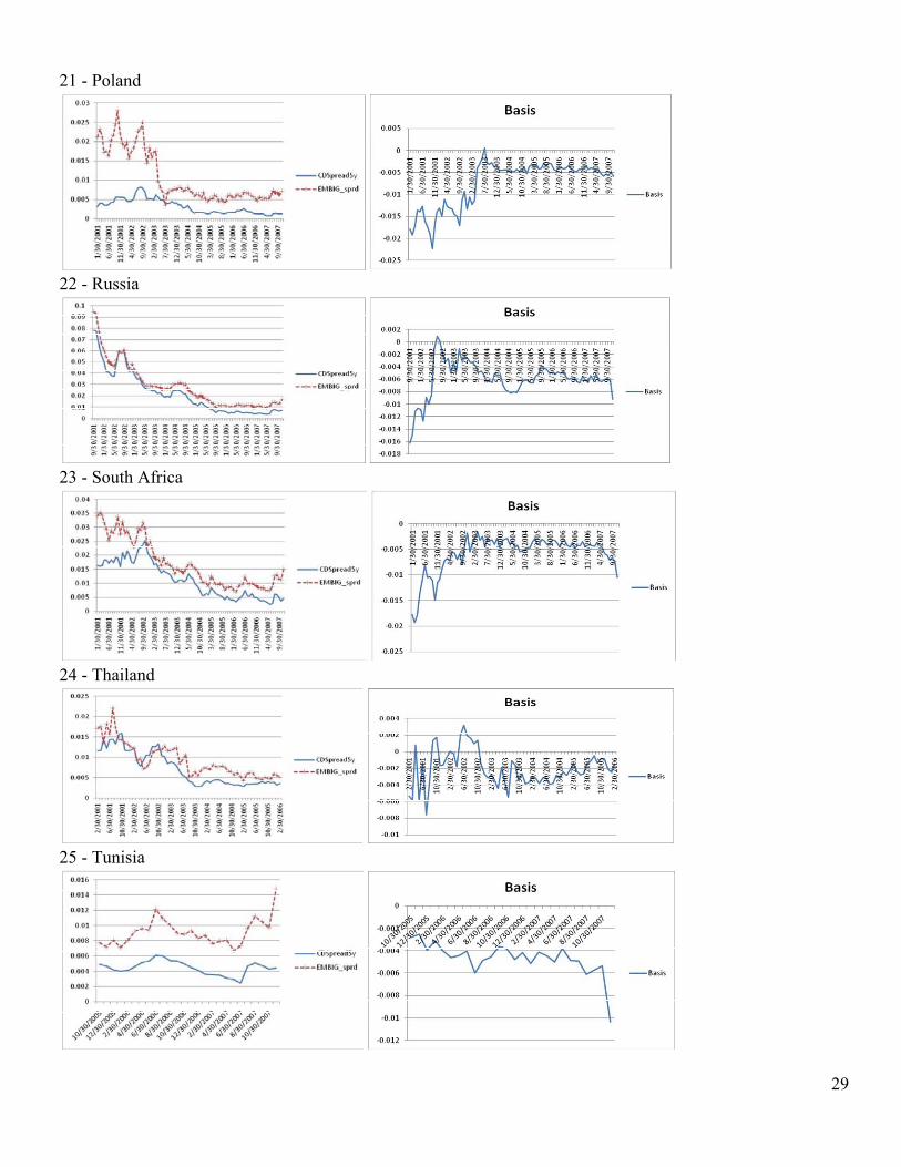
1 - First, we perform Augmented Dickey-Fuller (ADF) with Schwarz Criterion (SC) lag length selection method, and confirm that the data is non-stationary so that we can proceed with the cointegration test. We also specify a time trend in our model, since we observe that the spreads have been steadily decreasing since 2001. The model and the hypothesis tests are as follows. Detailed ADF tests up to 12 month lags can be found in Appendix III.

∆Y a a t βY C ∆Y C ∆Y … CP∆Y P e (1)

: 0, ,

: 0, ,

2 - After confirming the non-stationarity in the previous step, we can move on with the cointegration tests, to test the long-term relationship between the Bond and CDS markets. Initially, the following vector auto regression (VAR) model is constructed.

X A A X A X AP X P (2)

where, X = (2x1) vector of CDS and Bond Spreads, A = (2x1) vector of intercept terms

A = (2x1) vector of coefficient parameters = (2x1) vector of stochastic shocks that may or may not be correlated with each other

The cointegration test estimates the following form.

∆X δX ∑ R ∆X (3) The rank of the matrix is crucial since the term δX has to be stationary, i.e. I(0). In our case, the determinant of this matrix should be equal to zero, or the rows should be linearly dependent, in order for the cointegration relation to hold. If the two markets are cointegrated, the coefficient matrix has a rank of 1, and there exist 2x1 vectors α and β, such that δ αβT, where β is the cointegrating vector and is the vector of speed of adjustment parameters. The null and the alternative hypothesis take the following form.

: δ has a full rank of 2, the two spreads are not cointegrated : δ has a reduced rank of 1, the two spreads are cointegrated

In the cointegration tests, to determine the optimal lag length we used the pre-estimation version of STATA varsoc procedure which reports the final prediction error (FPE), Akaike's information criterion (AIC), Schwarz's Bayesian information criterion (SBIC), and the Hannan and Quinn information criterion (HQIC) for lag-order selection statistics for a series of vector autoregressions (VAR) of order maximum length up to 12 lags. When there is a conflict between the criterions, we used SBIC for optimal lag selection. After determining the optimal lag length, we performed Johansen's maximum likelihood cointegration rank test via

11

johans procedure in Stata. We observed that the results are very sensitive to the specified optimal lag lengths and maximum lag option. A short discussion and a sensitivity analysis related to lag-length selection procedures can be found in Table-1 in Part B. 3 - The final step is to estimate the Vector Error Correction Model (VECM) framework to find out the dynamic lead-lag relationship between the CDS and Bond markets.

CDS Bond z = I(0) (4)

∆∆ z +

∑ r , ∆CDS∑ r , ∆CDS

∑ k , ∆Bond∑ k , ∆Bond

(5)

The residuals of the first regression, cointegrating equation (4), should be stationary, I(0), in order for the two markets to be cointegrated. The second equation (5) is the VECM, which is a simultaneous regression equations matrix. In such a framework, one would mainly focus on the adjustment parameters. The alphas, speed of adjustment parameters, are interpreted as price discovery measures which give us an idea of the relative efficiency of the markets. In our case, by comparing the magnitudes and the signs of the alpha coefficients we can conclude whether the CDS or bond markets are leading in price discovery. The β matrix gives us the long run equilibrium relationship between sovereign CDS and bond markets. As an example, we can talk about Ukraine. In this case (after confirming that the data is non-stationary) the AIC and SBIC measures choose the same lag length for cointegration. The β and α matrices give us the following cointegrating equation and accompanying adjustment speeds.

CDS 1.22 Bond 0.01 = I (0)

0.5840.063

The adjustment coefficients tell us that CDS spreads adjust to close the gap, and bond spreads do not significantly adjust. In other words, this means that bond spreads are leading CDS spreads. A more interesting example is Brazil. In this case, we reject the cointegrating relation with SBIC statistic, whereas we cannot reject with AIC statistic. We believe that this finding is surprising and requires more in-depth research. We will focus on the lag selection methods in detail in the next section (Table-1 and Table-2). In evaluating the appropriate error correction mechanism, we make an important departure from Blanco et al. (2005) and Zhu (2006). In their study, the authors only consider significantly negative , and significantly positive , as the appropriate adjustments to correct the error. Enders (2004), on the other hand, argues that the gap can be closed with at least three different scenarios. We argue that there are five different cases that a positive gap can be closed, for a negative gap we would add another five scenarios similar to the ones below.

12

1 - An increase in CDS spread and a larger increase in bond spread 2 - A decrease in CDS spread and a smaller decrease in bond spread 3 - A decrease in CDS spread and an increase in bond spread 4 - A decrease in CDS spread and no change in bond spread 5 - No change CDS spread + an increase in bond spread In Table-3, we provide a very simple measure, , to check whether one of the five scenarios above occurs as an appropriate error correction mechanism. In any of the five cases, a positive value for will be enough for the appropriate error correction.

13

B - Time Series Analysis - Empirical Results B.1 Cointegration and the Long-Run Equilibrium Relationship Table - 1: Cointegration & Lag Length Selection

According to Akaike Information Criterion (AIC), we have 5 countries for which we cannot confirm the cointegration, the long-run equilibrium relationship. Namely, we have Colombia, El Salvador, Hungary, Malaysia, and Panama as the exceptions in cointegration tests. According to Schwarz's Bayesian information criterion (SBIC), we have only 3 countries that we cannot confirm the cointegration relation, Brazil, Hungary, and Turkey. Reviewing the literature on the lag selection procedures, we have Blanco et al. (2005) and Euro Bond Market Study (ECB, 2004) using AIC measure. Whereas Zhu (2006) and Norden and Weber (2004) use both AIC and SBIC. On the other hand, Chan-Lau & Kim (IMF, 2004) and Ammer & Cai (FRB, 2007) favor SBIC. Lastly, we have Stata Time Series Manual (Release 9) favoring SBIC and HQIC over FPE and AIC based on the discussion of Lutkepohl (1993). Lutkepohl asserts that SBIC and HQIC provides consistent estimates of the true lag order, whereas AIC and FPE will overestimate the true lag order with a positive probability. At this point, we believe that it would not make any difference for corporate studies to use AIC or SBIC since both measures will give approximately the same results. That is probably why these studies did not emphasize the lag length selection procedures as an important part of their discussion. However, for the sovereign case we need to choose one measure over the others since they do not necessarily yield the same results.

5 YEAR CDS & EMBIG SPREADSTIME ‐ SERIES ANALYSIS SUMMARY

Johansen FPE Johansen AIC Johansen HQIC Johansen SBICCountries #obs cds #lags bond #lags Cointegration #lags Cointegration #lags Cointegration #lags Cointegration #lags

1 BRAZIL 1/30/2001 ‐ 11/30/2007 83 no 3 no 4 yes 11 yes 12 yes 11 no 42 BULGARIA 2/30/2001 ‐ 11/30/2007 82 no 11 no 2 yes 12 yes 12 yes 12 yes 13 CHILE 2/30/2002 ‐ 11/30/2007 70 no 4 no 1 yes 9 yes 9 no 4 yes 14 CHINA 1/30/2001 ‐ 11/30/2007 83 no 1 no 1 yes 1 yes 1 yes 1 yes 15 COLOMBIA 3/30/2001 ‐ 11/30/2007 81 no 1 no 1 no 9 no 9 yes 1 yes 16 CROATIA 1/30/2001 ‐ 5/30/2004 41 no 1 no 1 yes 10 yes 12 yes 12 yes 17 DOMINICAN REP. 6/30/2003 ‐ 11/30/2007 54 no 2 no 1 yes 12 yes 12 yes 2 yes 28 ECUADOR 1/30/2004 ‐ 11/30/2007 47 no 2 no 1 yes 1 yes 1 yes 1 yes 19 EGYPT 3/30/2002 ‐ 11/30/2007 69 no 7 no 1 yes 6 yes 6 yes 6 yes 2

10 EL SALVADOR 4/30/2003 ‐ 11/30/2007 56 no 1 no 1 no 2 no 2 yes 1 yes 111 HUNGARY 2/30/2001 ‐ 11/30/2007 82 no 1 no 1 no 1 no 2 no 1 no 112 KOREA 3/30/2001 ‐ 3/30/2004 37 no 1 no 1 yes 11 yes 12 yes 12 yes 1213 LEBANON 3/30/2003 ‐ 11/30/2007 57 no 1 no 1 yes 1 yes 1 yes 1 yes 114 MALAYSIA 4/30/2001 ‐ 11/30/2007 80 no 3 no 1 no 9 no 9 yes 1 yes 115 MEXICO 1/30/2001 ‐ 11/30/2007 83 no 1 no 1 yes 9 yes 11 yes 2 yes 116 MOROCCO 3/30/2001 ‐ 10/30/2006 68 no 1 no 1 yes 2 yes 2 yes 2 yes 117 PAKISTAN 6/30/2004 ‐ 11/30/2007 42 no 1 no 1 yes 1 yes 12 yes 12 yes 118 PANAMA 2/30/2002 ‐ 11/30/2007 70 no 1 no 2 no 2 no 2 no 2 yes 119 PERU 2/30/2002 ‐ 11/30/2007 70 no 1 no 1 yes 1 yes 1 yes 1 yes 120 PHILIPPINES 3/30/2001 ‐ 11/30/2007 81 no 1 no 1 yes 1 yes 1 yes 1 yes 121 POLAND 1/30/2001 ‐ 11/30/2007 83 no 5 no 1 yes 8 yes 12 yes 8 yes 122 RUSSIA 1/30/2002 ‐ 9/30/2007 73 no 1 no 1 yes 9 yes 9 no 6 yes 123 SOUTH AFRICA 1/30/2001 ‐ 11/30/2007 83 no 1 no 1 yes 1 yes 1 yes 1 yes 124 THAILAND 1/30/2002 ‐ 2/30/2006 61 no 1 no 1 no 10 yes 12 yes 1 yes 125 TUNISIA 10/30/2005 ‐ 11/30/2007 26 no 1 no 1 yes 8 yes 7 yes 7 yes 726 TURKEY 1/30/2001 ‐ 11/30/2007 83 no 1 no 1 yes 12 yes 12 yes 5 no 227 UKRAINE 7/30/2003 ‐ 11/30/2007 53 no 1 no 1 yes 1 yes 1 yes 1 yes 128 URUGUAY 1/30/2005 ‐ 11/30/2007 35 no 1 no 1 yes 1 yes 1 yes 1 yes 129 VENEZUELA 2/30/2001 ‐ 11/30/2007 82 no 1 no 1 yes 1 yes 1 yes 1 yes 130 VIETNAM 11/30/2005 ‐ 11/30/2007 25 no 1 no 1 yes 7 yes 8 yes 8 yes 8

CDS & EMBIG Spreads ADF stationarityData Coverage

14

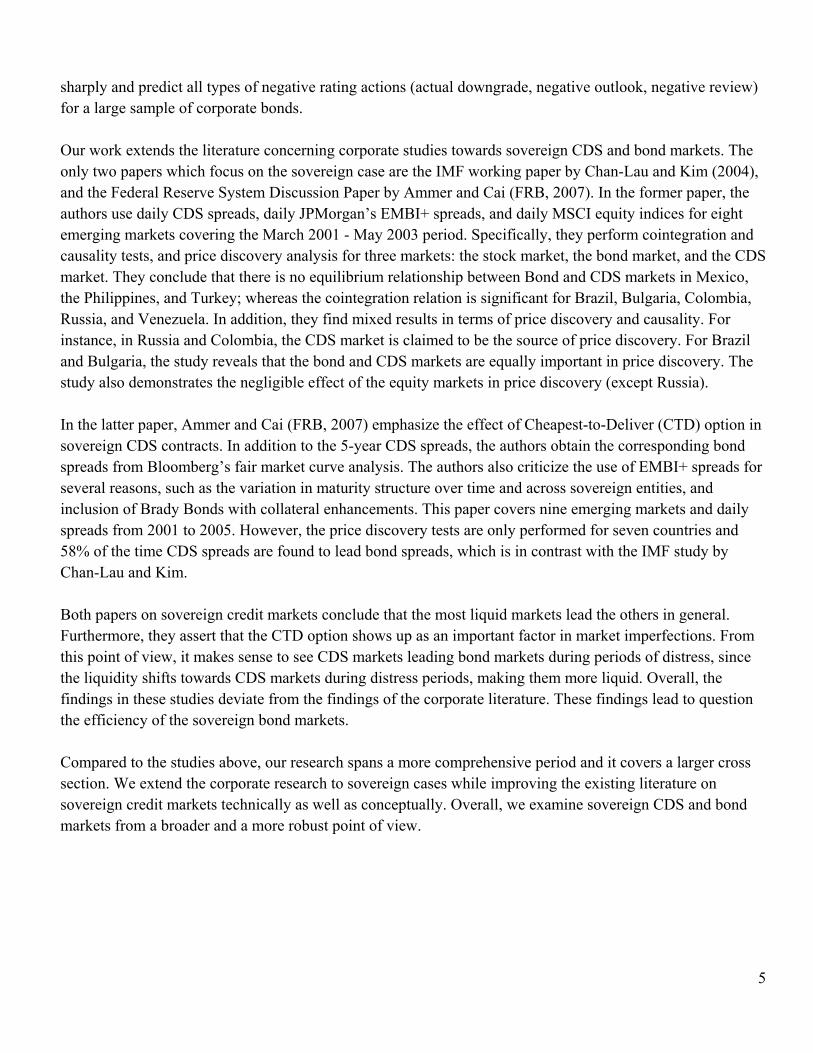
Zhu (2006) claims that the AIC and SBIC measures generally point to one or two periods with a maximum of five days as the optimal lag length. Similarly, Norden and Weber (2004), with daily and weekly frequencies of data, mention that the maximum lag order for daily frequency is 5 and for weekly frequency is 2. The IMF study by Chan-Lau and Kim use 1, 5, 10, and 20 days lag lengths to compare their results. Considering the corporate studies and the sovereign study by IMF, it makes more sense to have a short (i.e. one or two months) optimal lag length. Accordingly, we prefer SBIC measure over other measures since this measure gives us shorter and reasonable lag lengths (Table-1). If we ignore the countries with very low number of observations (i.e. less than 40, Korea, Tunisia and Vietnam), generally we have one or two lags (except Brazil). After we conclude the discussion of lag-length selection procedures and cointegration among the sovereign CDS and bond markets, our third and last step is to move on with the VECM framework. Table-2 summarizes the whole discussion. It is important to note that the CDS markets are very new in the sovereign case, and it is very natural to see some countries deviating from the theoretical cointegrating relation. Namely, we have Brazil, Hungary, and Turkey as the three markets which are not in line with the theory. In general, one can count liquidity conditions, contract specifications (i.e. CTD), and investor base as the potential explanations for such deviations (Chan-Lau & Kim, IMF, 2004, and Ammer & Cai, FRB, 2007). However, we believe that the liquidity conditions need further exploration, and some microeconomic and behavioral aspects can be underlined. Concerning Brazil, the big jump in basis occurs in 2001-2003 period when the country suffered from a major financial crisis and political tensions related to presidential elections (Appendix II - Graph 1). We believe that this sharp increase is primarily due to the increasing concerns about the economy and rising demand for default protection (Deutsche Bank Research). One can also argue that the active players (hedge funds and short-term traders) in the CDS markets overreacted to news, whereas the more passive-committed players (i.e. major banks) did not panic since they form their strategies for the long-term. Concerning Hungary, (Appendix II - Graph 11), one can argue that the integration to the European Union in 2004 might uncover some issues related to the regulations. Additionally, the fiscal deficit and uncertainties in mid-2006 put a pressure on the economy, and the integration to the EU has not been very smooth for Hungary. In addition, deteriorating growth and weak domestic demand contributed to the undesired economic picture. More importantly, Hungary is recognized as falling behind regional peers in maintaining its overall business climate according to competitiveness measures (IMF Country Report, July 2007). All these factors can be combined to explain why the long-run equilibrium relation is rejected for Hungary. Concerning Turkey, the crisis with the following currency devaluation in 2001 and the continued financial uncertainties during the 2001-2003 period seemed to contribute to the irregularities in bond markets. Even though the IMF agreements have reduced the tensions, a large current-account deficit and heavy reliance on short-term capital inflows leave the economy vulnerable to sharp changes in investor sentiment (the Economist, Country Briefings, Turkey).

15

There is no doubt that a more in-depth research is required to learn the specific reasons for the deviations from the long-run equilibrium relation.1 All the factors mentioned above are reasons of macroeconomic instability and do not necessarily explain why bond and the CDS markets deviate from each other. A quick microeconomic explanation might be that the two markets are still segmented, and the investor base is completely separate. For the corporate world, the CDS market is dominated by hedge funds and Wall Street firms, whereas in cash (bond) markets we have longer-term investors such as mutual funds, insurance companies and pension funds (Ng and Lauricella, WSJ, May-23-2008). In other words, one can argue that the CDS market is dominated by active money managers who focus majorly on the short-run, whereas bond investors are more dedicated, and less prone to speculation. For the sovereign case, we can tell a similar story and point to the different players and their short-run vs. long-run motivations in explaining some of the anomalies. In addition, the measures we use for CDS markets (5 Year CDS Premium) and Bond Markets (EMBIG) are not perfect matches, and the differences in the instruments and methodologies in calculating the two spreads might also account for some of the deviations. Therefore, a specific regulation or a specific bond issuance policy for a sovereign might well account for the disequilibrium in bond markets. B.2 VECM Framework and the Price Discovery Analysis Looking at the picture in Table-2, our first observation is that with SBIC, the number of countries (17) which have proper adjustment is larger compared to the number suggested by AIC (13). Second, we have numerous (8 with AIC, 4 with SBIC) countries in which the error correction works in an unexpected direction. We interpret this result as the outcome of market imperfections for those markets. Compared to the Chan-Lau Kim (IMF, 2004) study, our results are much stronger. In their study, which covers 2001-2003 period, the authors could not confirm the cointegration relationship in three (Mexico, Philippines, Turkey) out of eight emerging markets. In our study, we can see that in all countries the spreads are non-stationary, and in twenty-seven (with SBIC measure) out of thirty countries they are cointegrated with the exceptions of Brazil, Turkey, and Hungary. These results confirm that the sovereign CDS and bond markets have been developing, so that in the long-run they move in the same direction. However, in terms of market efficiency there are still some problems. Namely, we cannot see the expected error correction mechanism in some markets with our VECM framework. This finding is a sign that sovereign CDS and bond markets still have a long way to go to reach the corporate market efficiency levels.

1 We have also performed Granger Causality tests for the three countries we could not confirm the cointegration. We find no significant one-way causality in these cases. Results are available upon request.

16

Table - 2: Cointegration Equations & VECM Speed of Adjustment (Alpha) Coefficients

CDS Bond z = I(0)

∆∆ z +

∑ r , ∆CDS∑ r , ∆CDS

∑ k , ∆Bond∑ k , ∆Bond

5 YEAR CDS & EMBIG SPREADSCointegration and VECM Coefficients with Significance Levels

proper proper

Countries constant β1 α1 α2 adjustment constant β1 α1 α2 adjustment

1 BRAZIL 0.029 ‐1.490 *** ‐1.13 *** ‐0.64 *** yes no cointegration2 BULGARIA ‐0.003 0.006 ‐0.11 *** ‐0.09 ** yes 0.003 ‐0.823 *** ‐0.28 *** 0.14 yes3 CHILE ‐0.003 ‐0.083 ‐0.15 *** ‐0.17 *** no 0.012 ‐1.706 *** ‐0.21 *** 0.04 yes4 CHINA ‐0.001 ‐0.227 ‐0.13 *** ‐0.21 ** no ‐0.001 ‐0.227 ‐0.13 *** ‐0.21 ** no5 COLOMBIA no cointegration 0.013 ‐1.414 *** 0.12 0.34 *** yes6 CROATIA ‐0.011 0.059 ‐0.39 ‐0.72 ** no ‐0.030 1.508 ‐0.05 * ‐0.05 ** ?7 DOMINICAN REP. 0.017 ‐1.578 *** ‐1.50 *** 0.05 yes 0.021 ‐1.689 *** ‐0.81 *** 0.03 yes8 ECUADOR 0.018 ‐1.247 *** ‐0.44 *** ‐0.15 yes 0.018 ‐1.247 *** ‐0.44 *** ‐0.15 yes9 EGYPT 0.002 ‐1.408 *** ‐0.50 *** 0.02 yes 0.000 ‐1.137 *** ‐0.35 *** ‐0.18 *** yes

10 EL SALVADOR no cointegration 0.021 ‐1.635 *** ‐0.04 0.22 *** yes11 HUNGARY no cointegration no cointegration12 KOREA ‐0.006 ‐0.065 0.23 ‐0.49 ? ‐0.006 ‐0.065 0.23 ‐0.49 ?13 LEBANON ‐0.043 0.121 ‐0.16 *** ‐0.08 * yes ‐0.043 0.121 ‐0.16 *** ‐0.08 * yes14 MALAYSIA no cointegration 0.005 ‐0.887 *** ‐0.09 0.22 ?15 MEXICO 0.011 ‐1.161 *** ‐0.33 0.27 ? 0.010 ‐1.089 *** ‐0.16 0.10 ?16 MOROCCO 0.006 ‐1.196 *** ‐0.23 *** 0.21 ** yes 0.006 ‐1.136 *** ‐0.24 *** 0.08 yes17 PAKISTAN ‐0.031 0.421 ‐1.32 *** ‐1.42 *** no ‐0.002 ‐0.999 *** ‐0.41 * ‐0.05 yes18 PANAMA no cointegration 0.017 ‐1.420 *** ‐0.48 *** 0.03 yes19 PERU 0.006 ‐1.062 *** ‐0.29 * ‐0.12 yes 0.006 ‐1.062 *** ‐0.29 * ‐0.12 yes20 PHILIPPINES 0.008 ‐1.161 *** ‐0.10 0.11 ? 0.008 ‐1.161 *** ‐0.10 0.11 ?21 POLAND 0.000 ‐0.308 *** ‐0.29 *** ‐0.61 yes 0.000 ‐0.365 *** ‐0.11 *** 0.09 yes22 RUSSIA 0.007 ‐0.990 *** ‐0.86 *** ‐0.38 * yes 0.007 ‐1.146 *** 0.28 *** 0.40 *** yes23 SOUTH AFRICA 0.004 ‐0.990 *** ‐0.06 0.09 ? 0.004 ‐0.990 *** ‐0.06 0.09 ?24 THAILAND ‐0.083 16.300 *** ‐0.01 *** 0.00 yes 0.003 ‐1.128 *** ‐0.09 0.42 *** yes25 TUNISIA 0.016 ‐2.210 *** 1.04 *** 0.56 no 0.016 ‐2.210 *** 1.04 *** 0.56 no26 TURKEY 0.014 ‐1.637 *** 0.14 0.25 no no cointegration27 UKRAINE 0.006 ‐1.219 *** ‐0.58 *** ‐0.06 yes 0.006 ‐1.219 *** ‐0.58 *** ‐0.06 yes28 URUGUAY 0.014 ‐1.335 *** ‐0.23 0.40 ** yes 0.014 ‐1.335 *** ‐0.23 0.40 ** yes29 VENEZUELA 0.026 ‐1.439 *** ‐0.22 ‐0.28 no 0.026 ‐1.439 *** ‐0.22 ‐0.28 no30 VIETNAM 0.006 ‐0.994 *** 2.27 *** 7.22 ** no 0.006 ‐0.994 *** 2.27 *** 7.22 ** no

> Cointegration hypotheses testing performed according to Trace Statistic yes = 13/30 yes = 17/30

SBIC ‐ Cointegrating EquationAIC ‐ Cointegrating Equation AIC ‐ VECM SBIC ‐ VECM

17

B.3 A New Price Discovery Measure Blanco et al. (2005) and Zhu (2006) suggest Gonzalo-Granger (GG) measure (1995) as a scale for the causality relation between CDS and Bond Markets. The measure is simply given as / . If GG is less than 0.5 we can conclude that the Bond markets lead CDS markets in price discovery. If GG is larger than 0.5, we can conclude that the CDS markets lead Bond markets in price discovery. However, the GG measure would not give us meaningful results if is not significantly negative, and is not significantly positive. As noted earlier, we argue that this measure is only appropriate for highly efficient markets. For the sovereign case, we suggest to accept any case out of our five possible scenarios if the coefficients work in an error correcting direction. As a new and comprehensive measure, we suggest (ignoring the significance levels of the coefficients) to check for the correct sign of adjustment. For instance, if the error at previous time period is positive, the measure should be positive for the gap to close in any of the five scenarios we discussed earlier. Similarly, if the error is negative, again the measure should be positive for the gap to close. So, regardless of the sign of the error at time t-1, measure should be positive for the error correction mechanism to work properly. Table-3 reports the values. With the SBIC measure as a reference, 5 countries out of 27, China, Croatia, Korea, Tunisia, and Venezuela, the price discovery mechanism is not appropriate and we observe inefficiency in sovereign credit markets. In 14 cases (with SBIC), we have CDS spreads significantly adjusting (decrease) in the expected direction. Whereas we have only 6 cases in which Bond spreads significantly adjust (increase) to correct the error. These results tell us that, in general, CDS spreads adjust to correct the errors; therefore bond spreads lead the CDS spreads. These results are partly in line with the paper by Chan-Lau & Kim (IMF, 2004). The authors note that the bond market may dominate price discovery because the banks are both the investors and the insurance (CDS) buyers. In addition, they assert that the CDS positions are more buy-and-hold natured since the banks do not trade these instruments, whereas bond markets are more active. They conclude that the bond market has a greater liquidity and trading volume, therefore it leads the CDS market. As a footnote, the authors note that the CDS markets price the default risk better in times of financial crises, therefore one might argue that the CDS spreads should lead bond spreads during market turbulence.

18

Table - 3: A New Price Discovery Measure

VECM ‐ Appropriate Error Correction Appropriate AppropriateAIC Error SBIC Error

Countries constant β1 α1 α2 α2‐α1 Correction constant β1 α1 α2 α2‐α1 Correction

1 BRAZIL 0.029 ‐1.490 *** ‐1.13 *** ‐0.64 *** 0.49 yes no cointegration2 BULGARIA ‐0.003 0.006 ‐0.11 *** ‐0.09 ** 0.02 yes 0.003 ‐0.823 *** ‐0.28 *** 0.14 0.42 yes3 CHILE ‐0.003 ‐0.083 ‐0.15 *** ‐0.17 *** ‐0.02 no 0.012 ‐1.706 *** ‐0.21 *** 0.04 0.25 yes4 CHINA ‐0.001 ‐0.227 ‐0.13 *** ‐0.21 ** ‐0.08 no ‐0.001 ‐0.227 ‐0.13 *** ‐0.21 ** ‐0.08 no5 COLOMBIA no cointegration 0.013 ‐1.414 *** 0.12 0.34 *** 0.22 yes6 CROATIA ‐0.011 0.059 ‐0.39 ‐0.72 ** ‐0.33 no ‐0.030 1.508 ‐0.05 * ‐0.05 ** ‐0.003 no7 DOMINICAN REP. 0.017 ‐1.578 *** ‐1.50 *** 0.05 1.55 yes 0.021 ‐1.689 *** ‐0.81 *** 0.03 0.84 yes8 ECUADOR 0.018 ‐1.247 *** ‐0.44 *** ‐0.15 0.29 yes 0.018 ‐1.247 *** ‐0.44 *** ‐0.15 0.29 yes9 EGYPT 0.002 ‐1.408 *** ‐0.50 *** 0.02 0.52 yes 0.000 ‐1.137 *** ‐0.35 *** ‐0.18 *** 0.18 yes

10 EL SALVADOR no cointegration 0.021 ‐1.635 *** ‐0.04 0.22 *** 0.26 yes11 HUNGARY no cointegration no cointegration12 KOREA ‐0.006 ‐0.065 0.23 ‐0.49 ‐0.71 no ‐0.006 ‐0.065 0.23 ‐0.49 ‐0.71 no13 LEBANON ‐0.043 0.121 ‐0.16 *** ‐0.08 * 0.08 yes ‐0.043 0.121 ‐0.16 *** ‐0.08 * 0.08 yes14 MALAYSIA no cointegration 0.005 ‐0.887 *** ‐0.09 0.22 0.31 yes15 MEXICO 0.011 ‐1.161 *** ‐0.33 0.27 0.60 yes 0.010 ‐1.089 *** ‐0.16 0.10 0.27 yes16 MOROCCO 0.006 ‐1.196 *** ‐0.23 *** 0.21 ** 0.44 yes 0.006 ‐1.136 *** ‐0.24 *** 0.08 0.31 yes17 PAKISTAN ‐0.031 0.421 ‐1.32 *** ‐1.42 *** ‐0.10 no ‐0.002 ‐0.999 *** ‐0.41 * ‐0.05 0.36 yes18 PANAMA no cointegration 0.017 ‐1.420 *** ‐0.48 *** 0.03 0.51 yes19 PERU 0.006 ‐1.062 *** ‐0.29 * ‐0.12 0.18 yes 0.006 ‐1.062 *** ‐0.29 * ‐0.12 0.18 yes20 PHILIPPINES 0.008 ‐1.161 *** ‐0.10 0.11 0.21 yes 0.008 ‐1.161 *** ‐0.10 0.11 0.21 yes21 POLAND 0.000 ‐0.308 *** ‐0.29 *** ‐0.61 ‐0.32 no 0.000 ‐0.365 *** ‐0.11 *** 0.09 0.19 yes22 RUSSIA 0.007 ‐0.990 *** ‐0.86 *** ‐0.38 * 0.48 yes 0.007 ‐1.146 *** 0.28 *** 0.40 *** 0.12 yes23 SOUTH AFRICA 0.004 ‐0.990 *** ‐0.06 0.09 0.15 yes 0.004 ‐0.990 *** ‐0.06 0.09 0.15 yes24 THAILAND ‐0.083 16.300 *** ‐0.01 *** 0.00 0.003 yes 0.003 ‐1.128 *** ‐0.09 0.42 *** 0.51 yes25 TUNISIA 0.016 ‐2.210 *** 1.04 *** 0.56 ‐0.48 no 0.016 ‐2.210 *** 1.04 *** 0.56 ‐0.48 no26 TURKEY 0.014 ‐1.637 *** 0.14 0.25 0.11 yes no cointegration27 UKRAINE 0.006 ‐1.219 *** ‐0.58 *** ‐0.06 0.52 yes 0.006 ‐1.219 *** ‐0.58 *** ‐0.06 0.52 yes28 URUGUAY 0.014 ‐1.335 *** ‐0.23 0.40 ** 0.63 yes 0.014 ‐1.335 *** ‐0.23 0.40 ** 0.63 yes29 VENEZUELA 0.026 ‐1.439 *** ‐0.22 ‐0.28 ‐0.05 no 0.026 ‐1.439 *** ‐0.22 ‐0.28 ‐0.05 no30 VIETNAM 0.006 ‐0.994 *** 2.27 *** 7.22 ** 4.94 yes 0.006 ‐0.994 *** 2.27 *** 7.22 ** 4.94 yes

AIC ‐ Cointegrating Equation AIC ‐ VECM SBIC ‐ Cointegrating Equation SBIC ‐ VECM

19

6 - Conclusions and Further Research

In this paper, we showed that the ties between sovereign CDS and bond markets have strengthened substantially in 2001-2007 period compared to earlier periods. Our analysis extended the literature with three major contributions. First, we have looked at a period and a cross section that has never examined before. This has become possible through the use of EMBIG which uses an expanded sample compared to the earlier studies which made use of EMBI+ or corresponding bond spreads. Second, we questioned the long-run equilibrium relationship between the two markets. Consequently, we have shown that sovereign CDS and bond markets have been more and more integrated. At first, we measured the improvement via cointegration tests, and confirmed that twenty-seven out of thirty countries (90%) have a long-run equilibrium relationship between bond and CDS markets. A measure for market efficiency is the condition that the derivative markets dominate the asset markets in price discovery. For example, the changes in the value of a call option should give an early signal for the direction of the underlying stock price; therefore the call option price should be leading the underlying stock price. In our case the CDS markets should be leading the bond markets since the market view is more frequently reflected via CDS spreads. Even though the recent studies confirmed that this principle holds in the US and European corporate markets (Zhu, 2006, Norden and Weber, 2004), the findings in sovereign context are in sharp contrast. However, our results are in line with Chan-Lau and Kim’s (2004) discussion. We show that bond markets lead CDS markets in general (48% of the time), but lag CDS spreads in some cases (22% of the time). Even though we can argue that the efficiency of sovereign markets have improved over the 2001-2007 period, the bond market still matters more because of its higher liquidity and trading volume. Third, we improved the time-series econometric analysis. Specifically, we extended the adjustment mechanism to more than two possible scenarios, and we created a simple measure to check for the appropriate error correction. Additionally, we provided an extensive sensitivity analysis for the lag length selection procedures, and argued that the SBIC measure is more robust compared to AIC for the sovereign case. There are a few candidates for explaining the deviation of sovereign markets from corporate markets in terms of efficiency. First, the no-arbitrage assumptions do not perfectly hold in sovereign markets. For instance, it is not possible to short the sovereign bonds in many cases. This is also pointed out by Blanco et al. (2005) with the emphasis on non-zero repo costs. Second, the contract specifications matter. As Blanco et al. (2005) and Chan-Lau & Kim (2004) asserted, the cheapest-to-deliver option (CTD) has a significant effect on the behavior of the markets. Third, shifts in liquidity are also a common factor mentioned in most of the studies. Moreover, it is important to keep in mind that the EMBIG spreads are only proxies for five year sovereign bond spreads. In addition, the results are still sensitive to the specific instruments and methods used by JP Morgan in calculating the EMBIG. The calculation of the EMBIG spread for each sovereign involves accumulating Brady Bonds, Eurobonds, traded loans, and local market debt instruments into the same pool. Unfortunately, we do not have access to the specific weights of these debt instruments in the pool used to calculate for each sovereign bond spread. An uneven composition in these pools might as well lead to some anomalies.

20

There is no doubt that our study can be improved in various directions. First, acquiring a daily frequency data would be desirable to check for the robustness of our results. In addition, the VAR modeling can be extended with various variables such as stock market indices, exchange rates or global factors, such as VIX. In addition, case studies can be performed to see anomalies such as political instability or dependence on commodity prices in different countries. Lastly, the incentives in international finance and the impact of the contract specifications can be examined. Some sovereigns have begun to issue bonds with Collective Action Clauses (CAC) to prevent the moral hazard and deadweight losses in the international finance paradigm (Eichengreen, 2003). A closer look at the contract specifications, i.e. whether the sovereign bond issue has CAC mechanism or not, might as well lead to interesting findings.

21

REFERENCES

Amato, Remolona. (2003). The Credit Spread Puzzle. BIS Quarterly Review

Ammer, Cai. (2007). Sovereign CDS and Bond Pricing Dynamics in Emerging Markets: Does the Cheapest-to-Deliver Option Matter? Federal Reserve Board. SSRN.

Andritzky. (2006) Sovereign Default Risk Valuation. Springer.

Blanco, Brennan, Marsh. (2005). An Empirical Analysis of the Dynamic Relation between Investment Grade Bonds and Credit Default Swaps. The Journal of Finance.

Chan-Lau, Kim. (2004). Equity Prices, Credit Default Swaps, and Bond Spreads in Emerging Markets. IMF. SSRN.

Cavanagh, Long. (1999). Introducing the J.P. Morgan Emerging Markets Bond Index Global (EMBI Global).

Deutsche Bank Research. Financial Market Monitoring. How do CDS spreads compare to bond spreads?

Duffie. (1998). Credit Swap Valuation. Research Paper.

Duffie, Pedersen, Singleton. (2003). Modeling Sovereign Yield Spreads: A Case Study of Russian Debt. The Journal of Finance.

Eichengreen. 2003. Restructuring Sovereign Debt. Journal of Economic Perspectives.

Enders. (2004). Applied Econometric Time Series. Second Edition.

European Central Bank (2004). The Euro Bond Market Study.

Gonzalo, Granger. (1995). Estimation of Common Long-Memory Components in Cointegrated Systems. Journal of Business & Economic Statisctics.

Gaillard. (2007). Fitch, Moody's, and S&P's SovereignRatings, and EMBI Global Spreads: Lessons from 1993-2006. Des Sciences Fondation Nationale Politiques.

Hartelius. Kashiwase. Kodres. (2008). Emerging Market Spread Compression: Is it real or is it Liquidity? IMF. SSRN.

Hilscher. Nosbuch. (2007). Determinants of Sovereign Risk: Macroeconomic Fundamentals and Pricing of Sovereing Debt. Brandeis University. LSE.

Hull, Predescu, White. (2004). The Relationship between Credit Default Swap Spreads, Bond Yields, and Credit Rating Announcements. Journal of Banking and Finance.

Hull, White. (2000). Valuing Credit Default Swaps I: No Counter Party Default Risk

Jahjah. Yue. (2004). Exchange Rate Policy and Sovereign Bond Spreads in Developing Countries. IMF.

Johansen, Juselius (1990). Maximum Likelihood Estimation and Inference on Cointegration-with Applications to the Demand for money. Campos, Ericsson, Hendry (2005) General-to-Specific Modeling Volume I. International Library of Critical Writings in Econometrics.

Longstaff. Pan. Pederson. Singleton. (2007). How Sovereign is Sovereign Credit Risk ? NBER Working Paper. SSRN.

22

McGuire, Schrijvers. (2003). Common Factors in Emerging Market Spreads. BIS Quarterly Review.

Narag. (2004). The Term Structure and Default Risk in Emerging Markets. UCLA.

Norden, Weber. (2004). The comovement of Credit Default Swap, Bond and Stock Markets: An Empirical Analysis. CEPR.

Pan, Singleton. (2006). Default and Recovery Implicit in the Term Structure of Sovereign CDS Spreads. NBER.

Packer, Suthiphongchai. (2003). Sovereign Credit Default Swaps. BIS Quarterly Review.

Powell. Martinez. (2008). On Emerging Economy Sovereign Spreads and Ratings. Inter-American Development Bank.

Remolona. Scatigna. Wu. (2007). Interpreting Sovereign Spreads. BIS Quarterly Review

Singh. Andritzky. (2005). Overpricing in Emerging Market CDS Contracts: Some Evidence from Recent Distress Cases. IMF.

Singh. (2003). Are Credit Default Swap Spreads High in Emerging Markets? An Alternative Methodology for Proxying Recovery Value. IMF.

Singh. Andritzky. (2006) The Pricing of Credit Default Swaps During Distress. IMF.

Skinner, Nuri. (2007). Hedging Emerging Market Bonds and the Rise of the Credit Default Swap. International Review of Financial Analysis.

Sy. (2001). Emerging Market Bond Spreads and Sovereign Credit Ratings: Reconciling Market Views with Economic Fundamentals. IMF. SSRN

Sy. (2004). Rating the Rating Agencies: Anticipating Currency Crisis Or Debt Crisis? IMF. SSRN

Stata Time Series Reference Manual, Release 9 (2005). Stata Press.

Zhu. (2006). An Empirical Comparison of Credit Spreads between the Bond Market and the Credit Default Swap Market. Journal of Financial Services Research.

23

APPENDIX I – Literature Review

Date Authors Title of the Paper Data Major Conclusions Methodology

1 December 2003 McGuire & Schrijvers  Common Factors in Emerging  The changes in daily spreads, EMBIG The authors show that a common factor accounts for 1/3 of variation in the emerging market daily spreads,  Principal Component  AnalysisBIS Quarterly Review Market Spreads 15 Emerging Markets  remaining 2/3 attributed to the idiosyncratic factors. Factor Analysis

31 March 1997 to 18 June 2003 The common factor is highly correlated with (through PCA analysis) equity indices (S&P 500), OLS(25 Emerging Markets August 1999 to June 2003) US interest rates (10 year Treasury yield) and other measures (VIX index, High yield spread).(Investment Grade vs. Non‐Investment Grade ) The authors argue that this common factor is a reflection of the international investors' attitude toward risk. 

2 December 2007 Longstaff, Pan,  How Sovereign is Monthly CDS (5 year) Spread for 26 Countries Changes in Sovereign Credit Spreads are driven by changes in 3 common global factors;  Principal Component AnalysisPederson, Singleton Sovereign Credit Risk ? 23 Emerging + 3 Advanced Countries 1‐Global Financial Markets (US Corp. High Yield Spread) Credit Cluster AnalysisNBER SSRN Coverage: October 2000 ‐ May 2007 2‐ Global Risk Premia (VIX Index, Equity (S&P E/P) Risk Premium   OLS

Local Stock Market Returns (MSCI, S&P IFC), VIX 3‐Global Investment Flows (Bond & Equity Flows of Mutual Funds) Correlation AnalysisUS Stock Markets, Treasury & Corporate Yields as opposed to to country specific variables such as changes in local stock market return,  Sharpe Ratio AnalysisExchange Rates, Foreign Currency Reserves exchange rate, and foreign reserves which have a much smaller explanatory power.

3 January 2008 Powell, Martinez On Emerging Economy  Replicate AGR ‐ ECB 2007 Paper with (S&P, Moody's) Although a small number of economic fundamentals explain ratings reasonably well, variations/improvements OLSInter‐American  Sovereign Spreads and Ratings US Treasury, Corporate High Yield, VIX in those fundamentals are themselvers explained by a small number of global financial factors  Ordered Probit, LogitDevelopment Bank Coverage: 2004‐2007 Ratings do matter in determining EMBI Spreads even after controlling for the major macroeconomic variables. Principal Component Analysis

2006‐2007 Daily CDS(5yr) Spreads ‐ 20 Emerging Mrkts Growth, Fiscal Balance, and EU Membership effect EMBI spreads over and above ratings.Hausmann and Panizza Data Set for Debt  Changes in policies of FED and the ECB (injecting liquidity) served to reduce the CDS Spreads,Original Sin Variable, Volatility of Exchange Rate the news of Sub‐prime crisis was interpreted as a US centered problem, and did not effect the sovereign CDS spreads.

VIX and High Yield Variables Contribute to CDS spreads reduction.

4 January 2008 Hartelius, Kashiwase, Emerging Market Spread Sovereign Ratings/Outlooks, Moody's and S&P (monthly) Regress Bond Spreads over fundamentals (credit ratings) and  expectations/liquidity (US interest rates and volatility) OLSKodres Compression: 3 Month Fed Funds Futures Rates "Carry Trade", 90 Rolling Volatility measure for FFFR Fixed EffectsIMF Is it real or is it Liquidity? Daily/ Monthly observations from Jan 1991 to Feb 2007 VIX (CBOE); risk appetite

SSRN 30 Emerging Markets and US financial data,  Incorporates Outlooks (not a big imporovement)EMBI, EMBIG

5 March 2007 Remolona, Scatigna, Wu Interpreting Sovereign Spreads Corporate and Sovereign CDS Spreads (monthly) Sovereign Spreads can be divided into two major components; expected loss (default risk)  and risk premium (investors). OLSBIS Quarterly Review 26 Emerging Market Countries Risk premium is often larger part of the spread.

Ratings Implied Dafault Probabilities (mapping) Explain CDS Spreads with RIPD (or ratings), bond outstanding (liquidity), and VIX (global risk).Fitch, Moody's, S&P

6 October 2001 Sy Emerging Market Bond Spreads Perform a univariate regression (unbalanced panel)  Striking progression in the relationship between spreads and ratings from 1994 to 2001 Spearman Rank CorrelationIMF and Sovereign Credit Ratings:  using 17 EMBI+ Spreads and an average of  The relationship between the spreads and the ratings are less significant during period of crises (1997‐98) OLS

Reconciling Market Views with Moody's and S&P's long‐term foreign currency debt the spreads adjust asymmetrically when there are significant deviations from the estimated relationship: Residual AnalysisEconomic Fundamentals   from January 1994 to April 2001 when spreads are excessively low, the rating upgrade effect dominates the spread widening effectSSRN monthly observations when spreads are excessively high, the spread tightening effect is more important than the downgrade effect 

high spreads in Russia versus lower spreads in Asia in 1999‐2000 periods on a rating adjusted basispossibly because of liquidity conditions and broadening investor base for Asian Bonds.higher risk appetite of investors in 1994‐1997 periods

7 February 2004 Chan‐Lau, Kim. Equity Prices, Credit Default Swaps,  Daily CDS (from Deutsche Bank and Credit Trade) There is a strong correlation between CDS and bond spreads in Brazil, Bulgaria, Colombia, Russia, and Venezuela.  Cointegration Analysis IMF and Bond Spreads Bond (JPMorgan Chase EMBI+), and Equity prices (MSCI) No equilibrium price relationship between the CDS and bond markets in Mexico, the Philippines, and Turkey. Granger Causality Test

 in Emerging Markets from March 2001 to May 2003. Equity Markets, although very liquid, play a negligible role in price discovery except Russia. Price Discovery measuresSSRN 8 Emerging Markets CDS and bond spreads can diverge because of the "cheapest‐to‐deliver" option in the CDS contract, or because of  Hasbrouck (1995)

the relative liquidity in these two markets. Gonzalo & Granger (1995)In general, price discovery occurs in the most liquid market. Merton's ModelIn Emerging  Markets, however, the bond market tend to be more liquid, suggesting that the bond markets shouldalways dominate the bond markets. However, when default risk is high CDS market tend to price default risk betterthan the bond market. As a result, Bond Markets and CDS Markets tend to alternate in discovering the price.

8 March 2007 Norbert Gaillard Fitch, Moody's, and S&P's Sovereign  Unbalanced Panel 1 ‐ Moody's has more often disagreed with the market whereas Fitch Ratings have diverged more rarely.  OLSFondation Nationale  Ratings, and EMBI Global Spreads: Sovereign Ratings, JP Morgan EMBIG Spreads (DataStream) 2 ‐ Moody's adjust less to market spreads whereas S&P and Fitch generally try to stick to the spreads.Des Sciences  Lessons from 1993‐2006 32 Sovereigns 3 ‐ For all three agencies, there is an asymmetric adjustment of ratings, the agencies are more likely to downgrade Politiques. following the high spreads, whereas they are reluctant to upgrade when the spreads are very low. 

4 ‐  In line with Sy's results (2001), the relationship between ratings and market spreads is weaker in timesof market turbulence (1998) and in times of low risk aversion (2005‐2006). 5 ‐ Reactions of spreads to rating changes show that S&P downgrades and Moody's upgrades have the most significantimpact.

9 December 2007 Ammer, Cai Sovereign CDS and  Daily 5 Year Dollar Denominated Sovereign CDS CDS Markets seem to lead bond markets in price discovery in some instances, but lag bond prices in other cases. Johansen Cointegration VECMFederal Reserve Board Bond Pricing Dynamics in  from February 26, 2001 to March 31, 2005.  Relatively more liquid market tends to lead the other. Contract specifications is also another factor of deviation. Framework

Emerging Markets: Does the  9 Matching Emerging Mrkts 5 Yr Bond Spread (bloomberg) CTD Option is an important determinant of the CDS basis, and should be included in any pricing or risk model. Gonzalo and Granger Cheapest‐to‐Deliver Option  Price Discovery MeasureMatter? ‐ SSRN

10 2004 Hull, Predescu, White The relationship between credit default January 1998‐May 2002 CDS prices rise sharply, thus predict all three types of rating changes outlook)  well in advance Logistic RegressionJournal of Banking and swap spreads, bond yields, and credit Data on CDS of Corporations, Sovereigns, (actual downgrade, negative review, and negative outlook) McFadden's LRIFinance rating announcements and Quasi‐Sovereigns.

11 2004 SY Rating the Rating Agencies: 13 Emerging Markets, Monthly EMBI Spreads, 1990‐2002 Ratings do predict sovereign debt distress (spreads exceeding 1000 bp) cases.IMF Anticipating Currency Crisis Or Debt Crisis? ‐ SSRN

24

12 August 2004. Haibin Zhu.  An Empirical Comparison of credit  Daily US and EU Corporate Bond and CDS Markets  CDS Markets lead cash and bond markets in rating events and price adjustment in general. Cointegration TestBIS Working Papers spreads between the bond market  January 1st 1999 to December  31st 2002 Relative importance of CDS vs. Bond Markets depend on the specific firm, liquidity also matters. Granger Causality No 160  and the credit default swap market.  Panel Data Two Credit Markets are cointegrated in the long‐run. VECM

When swap rates are used as benchmark risk‐free rates, the price discrepancies between bond spreads and CDS EM Algorithmpremia are quite small.A number of explantory variables are suggested to explain basis spreads; lagged basis spread, changes in CDS spread,rating level and rating change, contractual arrangements, liquidity factors, macroeconomic conditions.Most of these factors (rating change being the most important)  seem to be significant except the last one.

13 June 2005 Singh, Andritzky,  Overpricing in Emerging Market CDS   Argentina, Brazil, Dominican Republic Restructurings result in high recovery values, much higher than the theoretical benchmark 20%. Contracts: Some Evidence 2001‐2004 period, unbalanced Thus the protection buyers should pay less for the CDS contract from Recent Distress Cases. EMBI and CDS spreads

14 December 2003.  Singh. IMF Are Credit Default Swap Spreads High in Emerging Markets? An Alternative Methodology for Proxying Recovery Value. 

15 November 2006 Andritzky & Singh, IMF The Pricing of Credit Default Swaps  1yr,3yr, 5yr CDS spreads, EMBIG country sub‐index,  the recovery rate for CDS contracts is much higher than traditionally assumed (25%) which drives "the basis"During Distress, and CTD bond from Brazil's distress in 2002‐2003 basis effects: delivery option, issuance of new bonds, short selling abilities, repo specialness (positive)

counterparty risk, bond illiquidity, funding risk (negative)most of these effects are hard to detect empiricallycompute implied recovery values from 3yr and 5yr CDS spreads and show that its significantly higher than 25%.Disagree with Pan & Singleton 2005 Paper on common global factors explaining a large part of variation in CDS spreads

16 November 2004 Jahjah & Yue Exchange Rate Policy and  51 Developing Countries over 1990‐2001 period There is a significant impact of exchange rate policy on sovereign bond issue decisions and bond spreads. OLSIMF Sovereign Bond Spreads Primary Bond Market Spreads Real Exchange rate overvaluation significantly increases sovereign bond issue probability and raises bond spreads

 in Developing Countries.  Exchange Rate Regime Classification (IMF) Exchange rate misalignment under a hard peg significantly increases bond spreads

17 November 2007 Hilscher, Nosbuch Determinants of Sovereign Risk 32 Emerging Markets, Emphasis on Volatility of Fundamentals, especially Terms of Trade and Gowth Volatlity. OLS, Logit RegressionBrandeis University Macroeconomic Fundamentals Daily  EMBIG from January 1994 to 2006 (or Annual Mean) Commodity (Exports) Prices LSE and Pricing of Sovereing Debt Annual Macroeconomic Variables 1994 to 2003 Very low R‐Squared values

25

APPENDIX II - 5 Year CDS Spreads and EMBIG Spreads over 2001 – 2007 Period 1 - Brazil

2 - Bulgaria

3 - Chile

4 - China

5 - Colombia

26

6 - Croatia

7 - Dominican Republic

8 - Ecuador

9 - Egypt

10 - El Salvador

27

11 - Hungary

12 - Korea

13 - Lebanon

14 - Malaysia

15 - Mexico

28

16 - Morocco

17 - Pakistan

18 - Panama

19 - Peru

20 – Philippines

29

21 - Poland

22 - Russia

23 - South Africa

24 - Thailand

25 - Tunisia

30

26 - Turkey

27 - Ukraine

28 - Uruguay

29 - Venezuela

30 - Vietnam

31

APPENDIX III - ADF Tests (with trend) for CDS and Bond Spreads (1 to 12 Lags – Monthly Observations)

BRAZIL BULGARIA CHILE CHINA

Augmented Dickey‐Fuller  for unit root         Number of obs   =        81 AugmentedDickey‐Full for unit root         Number of obs   =        80 Augmented Dickey‐Full for unit root         Number of obs   =        68 AugmentedDickey‐Full for unit root         Number of obs   =        815 YEAR CDS SPREADS 5 YEAR CDS SPREADS 5 YEAR CDS SPREADS 5 YEAR CDS SPREADS

interpolated Dickey‐Fuller interpolated Dickey‐Fuller interpolated Dickey‐Fuller Interpolated Dickey‐FullerTest 1% Critical 5% Critical 10% Critical Test 1% Critical 5% Critical 10% Critical Test 1% Critical 5% Critical 10% Critical Test 1% Critical 5% Critical 10% Critical

Statistic Value Value Value Statistic Value Value Value Statistic Value Value Value Statistic Value Value Valuelags lags lags lags

1 Z(t) ‐2.493 ‐4.082 ‐3.469 ‐3.161 1 Z(t) ‐1.132 ‐4.084 ‐3.47 ‐3.162 1 Z(t) ‐2.9 ‐4.11 ‐3.482 ‐3.169 1 Z(t) ‐4.859 ‐4.082 ‐3.469 ‐3.1612 Z(t) ‐3.343 ‐4.084 ‐3.47 ‐3.162 2 Z(t) ‐1.362 ‐4.086 ‐3.471 ‐3.163 2 Z(t) ‐2.763 ‐4.113 ‐3.483 ‐3.17 2 Z(t) ‐4.278 ‐4.084 ‐3.47 ‐3.1623 Z(t) ‐3.343 ‐4.084 ‐3.47 ‐3.162 3 Z(t) ‐1.594 ‐4.088 ‐3.472 ‐3.163 3 Z(t) ‐2.135 ‐4.115 ‐3.484 ‐3.17 3 Z(t) ‐3.034 ‐4.086 ‐3.471 ‐3.1634 Z(t) ‐3.127 ‐4.088 ‐3.472 ‐3.163 4 Z(t) ‐0.913 ‐4.091 ‐3.473 ‐3.164 4 Z(t) ‐2.074 ‐4.117 ‐3.485 ‐3.171 4 Z(t) ‐2.228 ‐4.088 ‐3.472 ‐3.1635 Z(t) ‐2.823 ‐4.091 ‐3.473 ‐3.164 5 Z(t) ‐1.003 ‐4.093 ‐3.474 ‐3.164 5 Z(t) ‐1.785 ‐4.119 ‐3.486 ‐3.172 5 Z(t) ‐2.328 ‐4.091 ‐3.473 ‐3.1646 Z(t) ‐2.654 ‐4.093 ‐3.474 ‐3.164 6 Z(t) ‐0.827 ‐4.095 ‐3.475 ‐3.165 6 Z(t) ‐2.027 ‐4.121 ‐3.487 ‐3.172 6 Z(t) ‐2.946 ‐4.093 ‐3.474 ‐3.1647 Z(t) ‐2.531 ‐4.095 ‐3.475 ‐3.165 7 Z(t) ‐1.158 ‐4.097 ‐3.476 ‐3.166 7 Z(t) ‐4.993 ‐4.124 ‐3.488 ‐3.173 7 Z(t) ‐2.79 ‐4.095 ‐3.475 ‐3.1658 Z(t) ‐2.491 ‐4.097 ‐3.476 ‐3.166 8 Z(t) ‐1.619 ‐4.099 ‐3.477 ‐3.166 8 Z(t) ‐6.12 ‐4.126 ‐3.489 ‐3.173 8 Z(t) ‐3.956 ‐4.097 ‐3.476 ‐3.1669 Z(t) ‐2.683 ‐4.099 ‐3.477 ‐3.166 9 Z(t) ‐1.711 ‐4.102 ‐3.478 ‐3.167 9 Z(t) ‐6.377 ‐4.128 ‐3.49 ‐3.174 9 Z(t) ‐2.389 ‐4.099 ‐3.477 ‐3.166

10 Z(t) ‐2.979 ‐4.102 ‐3.478 ‐3.167 10 Z(t) ‐2.721 ‐4.104 ‐3.479 ‐3.167 10 Z(t) ‐3.127 ‐4.13 ‐3.491 ‐3.175 10 Z(t) ‐2.439 ‐4.102 ‐3.478 ‐3.16711 Z(t) ‐3.152 ‐4.104 ‐3.479 ‐3.167 11 Z(t) ‐0.511 ‐4.106 ‐3.48 ‐3.168 11 Z(t) ‐3.869 ‐4.132 ‐3.492 ‐3.175 11 Z(t) ‐2.12 ‐4.104 ‐3.479 ‐3.16712 Z(t) ‐3.319 ‐4.106 ‐3.48 ‐3.168 12 Z(t) ‐0.843 ‐4.108 ‐3.481 ‐3.169 12 Z(t) ‐3.194 ‐4.135 ‐3.493 ‐3.176 12 Z(t) ‐2.087 ‐4.106 ‐3.48 ‐3.168

SC test result for Lag Length Selection = 3 SC test result for Lag Length Selection = 11 SC test result for Lag Length Selection = 4 SC test result for Lag Length Selection = 1(Stata "varlag" procedure) (Stata "varlag" procedure) (Stata "varlag" procedure) (Stata "varlag" procedure)EMBIG SPREADS EMBIG SPREADS EMBIG SPREADS EMBIG SPREADS

1 Z(t) ‐2.408 ‐4.082 ‐3.469 ‐3.161 1 Z(t) ‐1.858 ‐4.084 ‐3.47 ‐3.162 1 Z(t) ‐0.811 ‐4.11 ‐3.482 ‐3.169 1 Z(t) ‐1.819 ‐4.082 ‐3.469 ‐3.1612 Z(t) ‐3.001 ‐4.084 ‐3.47 ‐3.162 2 Z(t) ‐2.421 ‐4.086 ‐3.471 ‐3.163 2 Z(t) ‐0.7 ‐4.113 ‐3.483 ‐3.17 2 Z(t) ‐0.684 ‐4.084 ‐3.47 ‐3.1623 Z(t) ‐3.774 ‐4.086 ‐3.471 ‐3.163 3 Z(t) ‐2.282 ‐4.088 ‐3.472 ‐3.163 3 Z(t) ‐0.609 ‐4.115 ‐3.484 ‐3.17 3 Z(t) ‐0.458 ‐4.086 ‐3.471 ‐3.1634 Z(t) ‐3.266 ‐4.088 ‐3.472 ‐3.163 4 Z(t) ‐2.201 ‐4.091 ‐3.473 ‐3.164 4 Z(t) ‐0.599 ‐4.117 ‐3.485 ‐3.171 4 Z(t) 0.121 ‐4.088 ‐3.472 ‐3.1635 Z(t) ‐2.82 ‐4.091 ‐3.473 ‐3.164 5 Z(t) ‐2.622 ‐4.093 ‐3.474 ‐3.164 5 Z(t) ‐1.522 ‐4.119 ‐3.486 ‐3.172 5 Z(t) ‐0.462 ‐4.091 ‐3.473 ‐3.1646 Z(t) ‐2.675 ‐4.093 ‐3.474 ‐3.164 6 Z(t) ‐1.936 ‐4.095 ‐3.475 ‐3.165 6 Z(t) ‐1.032 ‐4.121 ‐3.487 ‐3.172 6 Z(t) ‐0.964 ‐4.093 ‐3.474 ‐3.1647 Z(t) ‐2.59 ‐4.095 ‐3.475 ‐3.165 7 Z(t) ‐4.06 ‐4.097 ‐3.476 ‐3.166 7 Z(t) ‐1.302 ‐4.124 ‐3.488 ‐3.173 7 Z(t) ‐1.307 ‐4.095 ‐3.475 ‐3.1658 Z(t) ‐2.272 ‐4.097 ‐3.476 ‐3.166 8 Z(t) ‐4.887 ‐4.099 ‐3.477 ‐3.166 8 Z(t) ‐2.441 ‐4.126 ‐3.489 ‐3.173 8 Z(t) ‐2.07 ‐4.097 ‐3.476 ‐3.1669 Z(t) ‐2.267 ‐4.099 ‐3.477 ‐3.166 9 Z(t) ‐3.343 ‐4.102 ‐3.478 ‐3.167 9 Z(t) ‐1.216 ‐4.128 ‐3.49 ‐3.174 9 Z(t) ‐1.372 ‐4.099 ‐3.477 ‐3.166

10 Z(t) ‐2.707 ‐4.102 ‐3.478 ‐3.167 10 Z(t) ‐2.076 ‐4.104 ‐3.479 ‐3.167 10 Z(t) ‐0.846 ‐4.13 ‐3.491 ‐3.175 10 Z(t) ‐0.23 ‐4.102 ‐3.478 ‐3.16711 Z(t) ‐3.002 ‐4.104 ‐3.479 ‐3.167 11 Z(t) ‐2.714 ‐4.106 ‐3.48 ‐3.168 11 Z(t) ‐0.812 ‐4.132 ‐3.492 ‐3.175 11 Z(t) ‐0.135 ‐4.104 ‐3.479 ‐3.16712 Z(t) ‐3.15 ‐4.106 ‐3.48 ‐3.168 12 Z(t) ‐1.435 ‐4.108 ‐3.481 ‐3.169 12 Z(t) ‐0.462 ‐4.135 ‐3.493 ‐3.176 12 Z(t) ‐0.085 ‐4.106 ‐3.48 ‐3.168

SC test result for Lag Length Selection = 4 SC test result for Lag Length Selection = 2 SC test result for Lag Length Selection = 1 SC test result for Lag Length Selection = 1

COLOMBIA CROATIA DOMINICAN ECUADOR

AugmentedDickey‐Full for unit root         Number of obs   =        81 AugmentedDickey‐Full for unit root         Number of obs   =        40 AugmentedDickey‐Full for unit root         Number of obs   =        81 AugmentedDickey‐Full for unit root         Number of obs   =        455 YEAR CDS SPREADS 5 YEAR CDS SPREADS 5 YEAR CDS SPREADS 5 YEAR CDS SPREADS

Interpolated Dickey‐Fuller Interpolated Dickey‐Fuller Interpolated Dickey‐Fuller Interpolated Dickey‐FullerTest 1% Critical 5% Critical 10% Critical Test 1% Critical 5% Critical 10% Critical Test 1% Critical 5% Critical 10% Critical Test 1% Critical 5% Critical 10% Critical

Statistic Value Value Value Statistic Value Value Value Statistic Value Value Value Statistic Value Value Valuelags lags lags lags

1 Z(t) ‐2.643 ‐4.086 ‐3.471 ‐3.163 1 Z(t) ‐2.211 ‐4.251 ‐3.544 ‐3.206 1 Z(t) ‐2.115 ‐4.146 ‐3.498 ‐3.179 1 Z(t) ‐3.197 ‐4.196 ‐3.52 ‐3.1922 Z(t) ‐3.243 ‐4.088 ‐3.472 ‐3.163 2 Z(t) ‐3.756 ‐4.26 ‐3.548 ‐3.209 2 Z(t) ‐2.486 ‐4.148 ‐3.499 ‐3.179 2 Z(t) ‐2.299 ‐4.205 ‐3.524 ‐3.1943 Z(t) ‐3.01 ‐4.091 ‐3.473 ‐3.164 3 Z(t) ‐3.702 ‐4.27 ‐3.552 ‐3.211 3 Z(t) ‐2.576 ‐4.15 ‐3.5 ‐3.18 3 Z(t) ‐2.227 ‐4.214 ‐3.528 ‐3.1974 Z(t) ‐2.375 ‐4.093 ‐3.474 ‐3.164 4 Z(t) ‐2.78 ‐4.279 ‐3.556 ‐3.214 4 Z(t) ‐2.531 ‐4.159 ‐3.504 ‐3.182 4 Z(t) ‐1.761 ‐4.224 ‐3.532 ‐3.1995 Z(t) ‐2.747 ‐4.095 ‐3.475 ‐3.165 5 Z(t) ‐2.162 ‐4.288 ‐3.56 ‐3.216 5 Z(t) ‐2.731 ‐4.168 ‐3.508 ‐3.185 5 Z(t) ‐1.688 ‐4.233 ‐3.536 ‐3.2026 Z(t) ‐3.399 ‐4.097 ‐3.476 ‐3.166 6 Z(t) ‐2.104 ‐4.297 ‐3.564 ‐3.218 6 Z(t) ‐3.097 ‐4.178 ‐3.512 ‐3.187 6 Z(t) ‐2.294 ‐4.242 ‐3.54 ‐3.2047 Z(t) ‐3.279 ‐4.099 ‐3.477 ‐3.166 7 Z(t) ‐1.941 ‐4.306 ‐3.568 ‐3.221 7 Z(t) ‐2.625 ‐4.187 ‐3.516 ‐3.19 7 Z(t) ‐2.197 ‐4.251 ‐3.544 ‐3.2068 Z(t) ‐3.299 ‐4.102 ‐3.478 ‐3.167 8 Z(t) ‐1.693 ‐4.316 ‐3.572 ‐3.223 8 Z(t) ‐2.837 ‐4.196 ‐3.52 ‐3.192 8 Z(t) ‐2.523 ‐4.26 ‐3.548 ‐3.2099 Z(t) ‐3.373 ‐4.104 ‐3.479 ‐3.167 9 Z(t) ‐2.212 ‐4.325 ‐3.576 ‐3.226 9 Z(t) ‐2.45 ‐4.205 ‐3.524 ‐3.194 9 Z(t) ‐2.492 ‐4.27 ‐3.552 ‐3.21110 Z(t) ‐3.169 ‐4.106 ‐3.48 ‐3.168 10 Z(t) ‐2.377 ‐4.334 ‐3.58 ‐3.228 10 Z(t) ‐2.856 ‐4.214 ‐3.528 ‐3.197 10 Z(t) ‐1.675 ‐4.279 ‐3.556 ‐3.21411 Z(t) ‐2.975 ‐4.108 ‐3.481 ‐3.169 11 Z(t) ‐2.049 ‐4.343 ‐3.584 ‐3.23 11 Z(t) ‐1.995 ‐4.224 ‐3.532 ‐3.199 11 Z(t) ‐0.798 ‐4.288 ‐3.56 ‐3.21612 Z(t) ‐4.007 ‐4.11 ‐3.482 ‐3.169 12 Z(t) ‐2.506 ‐4.352 ‐3.588 ‐3.233 12 Z(t) ‐1.621 ‐4.233 ‐3.536 ‐3.202 12 Z(t) ‐0.803 ‐4.297 ‐3.564 ‐3.218

SC test result for Lag Length Selection = 1 SC test result for Lag Length Selection = 1 SC test result for Lag Length Selection = 2 SC test result for Lag Length Selection = 2(Stata "varlag" procedure) (Stata "varlag" procedure) (Stata "varlag" procedure) (Stata "varlag" procedure)EMBIG SPREADS EMBIG SPREADS EMBIG SPREADS EMBIG SPREADS

1 Z(t) ‐3.084 ‐4.086 ‐3.471 ‐3.163 1 Z(t) ‐1.735 ‐4.251 ‐3.544 ‐3.206 1 Z(t) ‐2.429 ‐4.146 ‐3.498 ‐3.179 1 Z(t) ‐2.821 ‐4.196 ‐3.52 ‐3.1922 Z(t) ‐3.484 ‐4.088 ‐3.472 ‐3.163 2 Z(t) ‐1.621 ‐4.26 ‐3.548 ‐3.209 2 Z(t) ‐2.764 ‐4.148 ‐3.499 ‐3.179 2 Z(t) ‐2.708 ‐4.205 ‐3.524 ‐3.1943 Z(t) ‐2.985 ‐4.091 ‐3.473 ‐3.164 3 Z(t) ‐1.729 ‐4.27 ‐3.552 ‐3.211 3 Z(t) ‐2.495 ‐4.15 ‐3.5 ‐3.18 3 Z(t) ‐2.461 ‐4.214 ‐3.528 ‐3.1974 Z(t) ‐2.61 ‐4.093 ‐3.474 ‐3.164 4 Z(t) ‐1.487 ‐4.279 ‐3.556 ‐3.214 4 Z(t) ‐2.511 ‐4.159 ‐3.504 ‐3.182 4 Z(t) ‐2.254 ‐4.224 ‐3.532 ‐3.1995 Z(t) ‐3.305 ‐4.095 ‐3.475 ‐3.165 5 Z(t) ‐1.39 ‐4.288 ‐3.56 ‐3.216 5 Z(t) ‐2.352 ‐4.168 ‐3.508 ‐3.185 5 Z(t) ‐1.927 ‐4.233 ‐3.536 ‐3.2026 Z(t) ‐3.038 ‐4.097 ‐3.476 ‐3.166 6 Z(t) ‐0.765 ‐4.297 ‐3.564 ‐3.218 6 Z(t) ‐2.125 ‐4.178 ‐3.512 ‐3.187 6 Z(t) ‐2.358 ‐4.242 ‐3.54 ‐3.2047 Z(t) ‐2.975 ‐4.099 ‐3.477 ‐3.166 7 Z(t) ‐0.582 ‐4.306 ‐3.568 ‐3.221 7 Z(t) ‐1.949 ‐4.187 ‐3.516 ‐3.19 7 Z(t) ‐2.265 ‐4.251 ‐3.544 ‐3.2068 Z(t) ‐3.425 ‐4.102 ‐3.478 ‐3.167 8 Z(t) ‐0.553 ‐4.316 ‐3.572 ‐3.223 8 Z(t) ‐2.488 ‐4.196 ‐3.52 ‐3.192 8 Z(t) ‐2.104 ‐4.26 ‐3.548 ‐3.2099 Z(t) ‐3.263 ‐4.104 ‐3.479 ‐3.167 9 Z(t) ‐0.889 ‐4.325 ‐3.576 ‐3.226 9 Z(t) ‐2.412 ‐4.205 ‐3.524 ‐3.194 9 Z(t) ‐1.51 ‐4.27 ‐3.552 ‐3.21110 Z(t) ‐3.007 ‐4.106 ‐3.48 ‐3.168 10 Z(t) ‐2.011 ‐4.334 ‐3.58 ‐3.228 10 Z(t) ‐2.619 ‐4.214 ‐3.528 ‐3.197 10 Z(t) ‐1.116 ‐4.279 ‐3.556 ‐3.21411 Z(t) ‐2.99 ‐4.108 ‐3.481 ‐3.169 11 Z(t) ‐2.36 ‐4.343 ‐3.584 ‐3.23 11 Z(t) ‐1.127 ‐4.224 ‐3.532 ‐3.199 11 Z(t) ‐0.689 ‐4.288 ‐3.56 ‐3.21612 Z(t) ‐4.495 ‐4.11 ‐3.482 ‐3.169 12 Z(t) ‐2.275 ‐4.352 ‐3.588 ‐3.233 12 Z(t) ‐2.617 ‐4.233 ‐3.536 ‐3.202 12 Z(t) ‐1.156 ‐4.297 ‐3.564 ‐3.218

SC test result for Lag Length Selection = 1 SC test result for Lag Length Selection = 1 SC test result for Lag Length Selection = 1 SC test result for Lag Length Selection = 1

32

EGYPT ELSALVADOR HUNGARY KOREA

AugmentedDickey‐Full for unit root         Number of obs   =        67 AugmentedDickey‐Full for unit root         Number of obs   =        54 AugmentedDickey‐Full for unit root         Number of obs   =        79 AugmentedDickey‐Full for unit root         Number of obs   =        355 YEAR CDS SPREADS 5 YEAR CDS SPREADS 5 YEAR CDS SPREADS 5 YEAR CDS SPREADS

Interpolated Dickey‐Fuller Interpolated Dickey‐Fuller Interpolated Dickey‐Fuller Interpolated Dickey‐FullerTest 1% Critical 5% Critical 10% Critical Test 1% Critical 5% Critical 10% Critical Test 1% Critical 5% Critical 10% Critical Test 1% Critical 5% Critical 10% Critical

Statistic Value Value Value Statistic Value Value Value Statistic Value Value Value Statistic Value Value Valuelags lags lags lags

1 Z(t) ‐1.638 ‐4.113 ‐3.483 ‐3.17 1 Z(t) ‐1.528 ‐4.141 ‐3.496 ‐3.178 1 Z(t) ‐2.116 ‐4.091 ‐3.473 ‐3.164 1 Z(t) ‐2.629 ‐4.288 ‐3.56 ‐3.2162 Z(t) ‐1.715 ‐4.115 ‐3.484 ‐3.17 2 Z(t) ‐1.454 ‐4.143 ‐3.497 ‐3.178 2 Z(t) ‐1.932 ‐4.095 ‐3.475 ‐3.165 2 Z(t) ‐2.156 ‐4.297 ‐3.564 ‐3.2183 Z(t) ‐2.256 ‐4.117 ‐3.485 ‐3.171 3 Z(t) ‐1.215 ‐4.146 ‐3.498 ‐3.179 3 Z(t) ‐2.342 ‐4.099 ‐3.477 ‐3.166 3 Z(t) ‐1.813 ‐4.306 ‐3.568 ‐3.2214 Z(t) ‐2.424 ‐4.119 ‐3.486 ‐3.172 4 Z(t) ‐0.512 ‐4.148 ‐3.499 ‐3.179 4 Z(t) ‐1.931 ‐4.104 ‐3.479 ‐3.167 4 Z(t) ‐1.84 ‐4.316 ‐3.572 ‐3.2235 Z(t) ‐1.926 ‐4.121 ‐3.487 ‐3.172 5 Z(t) 0.26 ‐4.15 ‐3.5 ‐3.18 5 Z(t) ‐2.186 ‐4.108 ‐3.481 ‐3.169 5 Z(t) ‐1.74 ‐4.325 ‐3.576 ‐3.2266 Z(t) ‐2.004 ‐4.124 ‐3.488 ‐3.173 6 Z(t) 0.218 ‐4.159 ‐3.504 ‐3.182 6 Z(t) ‐2.404 ‐4.113 ‐3.483 ‐3.17 6 Z(t) ‐2.936 ‐4.334 ‐3.58 ‐3.2287 Z(t) ‐2.744 ‐4.126 ‐3.489 ‐3.173 7 Z(t) ‐0.161 ‐4.168 ‐3.508 ‐3.185 7 Z(t) ‐2.227 ‐4.117 ‐3.485 ‐3.171 7 Z(t) ‐2.428 ‐4.343 ‐3.584 ‐3.238 Z(t) ‐3.004 ‐4.128 ‐3.49 ‐3.174 8 Z(t) 0.311 ‐4.178 ‐3.512 ‐3.187 8 Z(t) ‐2.524 ‐4.121 ‐3.487 ‐3.172 8 Z(t) ‐2.456 ‐4.352 ‐3.588 ‐3.2339 Z(t) ‐2.469 ‐4.13 ‐3.491 ‐3.175 9 Z(t) ‐0.32 ‐4.187 ‐3.516 ‐3.19 9 Z(t) ‐1.791 ‐4.126 ‐3.489 ‐3.173 9 Z(t) ‐2.386 ‐4.362 ‐3.592 ‐3.235

10 Z(t) ‐1.484 ‐4.132 ‐3.492 ‐3.175 10 Z(t) ‐0.166 ‐4.196 ‐3.52 ‐3.192 10 Z(t) ‐1.698 ‐4.13 ‐3.491 ‐3.175 10 Z(t) ‐2.795 ‐4.371 ‐3.596 ‐3.23811 Z(t) ‐1.539 ‐4.135 ‐3.493 ‐3.176 11 Z(t) ‐0.027 ‐4.205 ‐3.524 ‐3.194 11 Z(t) ‐1.652 ‐4.132 ‐3.492 ‐3.175 11 Z(t) ‐2.48 ‐4.38 ‐3.6 ‐3.2412 Z(t) ‐2.31 ‐4.137 ‐3.494 ‐3.176 12 Z(t) ‐0.066 ‐4.214 ‐3.528 ‐3.197 12 Z(t) ‐1.559 ‐4.135 ‐3.493 ‐3.176 12 Z(t) ‐2.278 ‐4.38 ‐3.6 ‐3.24

SC test result for Lag Length Selection = 7 SC test result for Lag Length Selection = 1 SC test result for Lag Length Selection = 1 SC test result for Lag Length Selection = 1(Stata "varlag" procedure) (Stata "varlag" procedure) (Stata "varlag" procedure) (Stata "varlag" procedure)EMBIG SPREADS EMBIG SPREADS EMBIG SPREADS EMBIG SPREADS

1 Z(t) ‐0.575 ‐4.113 ‐3.483 ‐3.17 1 Z(t) ‐3.482 ‐4.141 ‐3.496 ‐3.178 1 Z(t) ‐2.341 ‐4.084 ‐3.47 ‐3.162 1 Z(t) ‐2.674 ‐4.288 ‐3.56 ‐3.2162 Z(t) ‐0.729 ‐4.115 ‐3.484 ‐3.17 2 Z(t) ‐3.325 ‐4.143 ‐3.497 ‐3.178 2 Z(t) ‐2.095 ‐4.086 ‐3.471 ‐3.163 2 Z(t) ‐1.735 ‐4.297 ‐3.564 ‐3.2183 Z(t) ‐1.411 ‐4.117 ‐3.485 ‐3.171 3 Z(t) ‐2.827 ‐4.146 ‐3.498 ‐3.179 3 Z(t) ‐1.799 ‐4.088 ‐3.472 ‐3.163 3 Z(t) ‐1.926 ‐4.306 ‐3.568 ‐3.2214 Z(t) ‐1.334 ‐4.119 ‐3.486 ‐3.172 4 Z(t) ‐2.766 ‐4.148 ‐3.499 ‐3.179 4 Z(t) ‐1.954 ‐4.091 ‐3.473 ‐3.164 4 Z(t) ‐1.602 ‐4.316 ‐3.572 ‐3.2235 Z(t) ‐1.605 ‐4.121 ‐3.487 ‐3.172 5 Z(t) ‐3.191 ‐4.15 ‐3.5 ‐3.18 5 Z(t) ‐1.644 ‐4.093 ‐3.474 ‐3.164 5 Z(t) ‐1.532 ‐4.325 ‐3.576 ‐3.2266 Z(t) ‐2.919 ‐4.124 ‐3.488 ‐3.173 6 Z(t) ‐3.143 ‐4.159 ‐3.504 ‐3.182 6 Z(t) ‐1.412 ‐4.095 ‐3.475 ‐3.165 6 Z(t) ‐2.169 ‐4.334 ‐3.58 ‐3.2287 Z(t) ‐2.59 ‐4.126 ‐3.489 ‐3.173 7 Z(t) ‐3.127 ‐4.168 ‐3.508 ‐3.185 7 Z(t) ‐1.013 ‐4.097 ‐3.476 ‐3.166 7 Z(t) ‐2.983 ‐4.343 ‐3.584 ‐3.238 Z(t) ‐1.882 ‐4.128 ‐3.49 ‐3.174 8 Z(t) ‐3.249 ‐4.178 ‐3.512 ‐3.187 8 Z(t) ‐1.125 ‐4.099 ‐3.477 ‐3.166 8 Z(t) ‐3.213 ‐4.352 ‐3.588 ‐3.2339 Z(t) ‐1.365 ‐4.13 ‐3.491 ‐3.175 9 Z(t) ‐3.656 ‐4.187 ‐3.516 ‐3.19 9 Z(t) ‐1.42 ‐4.102 ‐3.478 ‐3.167 9 Z(t) ‐2.417 ‐4.362 ‐3.592 ‐3.235

10 Z(t) ‐0.497 ‐4.132 ‐3.492 ‐3.175 10 Z(t) ‐3.027 ‐4.196 ‐3.52 ‐3.192 10 Z(t) ‐2.059 ‐4.104 ‐3.479 ‐3.167 10 Z(t) ‐2.709 ‐4.371 ‐3.596 ‐3.23811 Z(t) ‐1.03 ‐4.135 ‐3.493 ‐3.176 11 Z(t) ‐2.684 ‐4.205 ‐3.524 ‐3.194 11 Z(t) ‐2.084 ‐4.106 ‐3.48 ‐3.168 11 Z(t) ‐2.165 ‐4.38 ‐3.6 ‐3.2412 Z(t) ‐1.964 ‐4.137 ‐3.494 ‐3.176 12 Z(t) ‐2.34 ‐4.214 ‐3.528 ‐3.197 12 Z(t) ‐2.504 ‐4.108 ‐3.481 ‐3.169 12 Z(t) ‐1.427 ‐4.38 ‐3.6 ‐3.24

SC test result for Lag Length Selection = 1 SC test result for Lag Length Selection = 1 SC test result for Lag Length Selection = 1 SC test result for Lag Length Selection = 1

LEBANON MALAYSIA MEXICO MOROCCO

AugmentedDickey‐Full for unit root         Number of obs   =       55 AugmentedDickey‐Full for unit root         Number of obs   =       78 AugmentedDickey‐Full for unit root         Number of obs   =       81 AugmentedDickey‐Full for unit root         Number of obs   =       665 YEAR CDS SPREADS 5 YEAR CDS SPREADS 5 YEAR CDS SPREADS 5 YEAR CDS SPREADS

Interpolated Dickey‐Fuller Interpolated Dickey‐Fuller Interpolated Dickey‐Fuller Interpolated Dickey‐FullerTest 1% Critical 5% Critical 10% Critical Test 1% Critical 5% Critical 10% Critical Test 1% Critical 5% Critical 10% Critical Test 1% Critical 5% Critical 10% Critical

Statistic Value Value Value Statistic Value Value Value Statistic Value Value Value Statistic Value Value Valuelags lags lags lags

1 Z(t) ‐2.697 ‐4.139 ‐3.495 ‐3.177 1 Z(t) ‐2.024 ‐4.088 ‐3.472 ‐3.163 1 Z(t) ‐3.156 ‐4.082 ‐3.469 ‐3.161 1 Z(t) ‐2.159 ‐4.115 ‐3.484 ‐3.172 Z(t) ‐2.638 ‐4.141 ‐3.496 ‐3.178 2 Z(t) ‐1.276 ‐4.091 ‐3.473 ‐3.164 2 Z(t) ‐3.555 ‐4.084 ‐3.47 ‐3.162 2 Z(t) ‐2.327 ‐4.117 ‐3.485 ‐3.1713 Z(t) ‐1.959 ‐4.143 ‐3.497 ‐3.178 3 Z(t) ‐1.529 ‐4.093 ‐3.474 ‐3.164 3 Z(t) ‐3.012 ‐4.086 ‐3.471 ‐3.163 3 Z(t) ‐2.501 ‐4.119 ‐3.486 ‐3.1724 Z(t) ‐1.485 ‐4.146 ‐3.498 ‐3.179 4 Z(t) ‐1.216 ‐4.095 ‐3.475 ‐3.165 4 Z(t) ‐2.987 ‐4.088 ‐3.472 ‐3.163 4 Z(t) ‐2.877 ‐4.121 ‐3.487 ‐3.1725 Z(t) ‐1.666 ‐4.148 ‐3.499 ‐3.179 5 Z(t) ‐2.737 ‐4.097 ‐3.476 ‐3.166 5 Z(t) ‐2.948 ‐4.091 ‐3.473 ‐3.164 5 Z(t) ‐3.323 ‐4.124 ‐3.488 ‐3.1736 Z(t) ‐1.804 ‐4.15 ‐3.5 ‐3.18 6 Z(t) ‐1.754 ‐4.099 ‐3.477 ‐3.166 6 Z(t) ‐2.81 ‐4.093 ‐3.474 ‐3.164 6 Z(t) ‐1.533 ‐4.126 ‐3.489 ‐3.1737 Z(t) ‐1.457 ‐4.159 ‐3.504 ‐3.182 7 Z(t) ‐0.993 ‐4.102 ‐3.478 ‐3.167 7 Z(t) ‐2.421 ‐4.095 ‐3.475 ‐3.165 7 Z(t) ‐1.172 ‐4.128 ‐3.49 ‐3.1748 Z(t) ‐1.63 ‐4.168 ‐3.508 ‐3.185 8 Z(t) ‐0.679 ‐4.104 ‐3.479 ‐3.167 8 Z(t) ‐1.737 ‐4.097 ‐3.476 ‐3.166 8 Z(t) ‐1.235 ‐4.13 ‐3.491 ‐3.1759 Z(t) ‐1.332 ‐4.178 ‐3.512 ‐3.187 9 Z(t) ‐0.867 ‐4.106 ‐3.48 ‐3.168 9 Z(t) ‐1.616 ‐4.099 ‐3.477 ‐3.166 9 Z(t) ‐1.484 ‐4.132 ‐3.492 ‐3.175

10 Z(t) ‐0.91 ‐4.187 ‐3.516 ‐3.19 10 Z(t) ‐0.823 ‐4.108 ‐3.481 ‐3.169 10 Z(t) ‐1.978 ‐4.102 ‐3.478 ‐3.167 10 Z(t) ‐2.038 ‐4.135 ‐3.493 ‐3.17611 Z(t) ‐0.828 ‐4.196 ‐3.52 ‐3.192 11 Z(t) ‐0.626 ‐4.11 ‐3.482 ‐3.169 11 Z(t) ‐2.217 ‐4.104 ‐3.479 ‐3.167 11 Z(t) ‐2.167 ‐4.137 ‐3.494 ‐3.17612 Z(t) ‐0.663 ‐4.205 ‐3.524 ‐3.194 12 Z(t) ‐0.583 ‐4.113 ‐3.483 ‐3.17 12 Z(t) ‐2.373 ‐4.106 ‐3.48 ‐3.168 12 Z(t) ‐3.727 ‐4.139 ‐3.495 ‐3.177

SC test result for Lag Length Selection = 1 SC test result for Lag Length Selection = 3 SC test result for Lag Length Selection = 1 SC test result for Lag Length Selection = 1(Stata "varlag" procedure) (Stata "varlag" procedure) (Stata "varlag" procedure) (Stata "varlag" procedure)EMBIG SPREADS EMBIG SPREADS EMBIG SPREADS EMBIG SPREADS

1 Z(t) ‐1.289 ‐4.139 ‐3.495 ‐3.177 1 Z(t) ‐1.645 ‐4.088 ‐3.472 ‐3.163 1 Z(t) ‐3.233 ‐4.082 ‐3.469 ‐3.161 1 Z(t) ‐3.234 ‐4.115 ‐3.484 ‐3.172 Z(t) ‐0.921 ‐4.141 ‐3.496 ‐3.178 2 Z(t) ‐1.298 ‐4.091 ‐3.473 ‐3.164 2 Z(t) ‐3.355 ‐4.084 ‐3.47 ‐3.162 2 Z(t) ‐3.113 ‐4.117 ‐3.485 ‐3.1713 Z(t) ‐0.903 ‐4.143 ‐3.497 ‐3.178 3 Z(t) ‐1.873 ‐4.093 ‐3.474 ‐3.164 3 Z(t) ‐3.048 ‐4.086 ‐3.471 ‐3.163 3 Z(t) ‐3.038 ‐4.119 ‐3.486 ‐3.1724 Z(t) ‐0.674 ‐4.146 ‐3.498 ‐3.179 4 Z(t) ‐1.188 ‐4.095 ‐3.475 ‐3.165 4 Z(t) ‐2.283 ‐4.088 ‐3.472 ‐3.163 4 Z(t) ‐2.456 ‐4.121 ‐3.487 ‐3.1725 Z(t) ‐0.884 ‐4.148 ‐3.499 ‐3.179 5 Z(t) ‐2.786 ‐4.097 ‐3.476 ‐3.166 5 Z(t) ‐2.439 ‐4.091 ‐3.473 ‐3.164 5 Z(t) ‐1.899 ‐4.124 ‐3.488 ‐3.1736 Z(t) ‐1.113 ‐4.15 ‐3.5 ‐3.18 6 Z(t) ‐2.279 ‐4.099 ‐3.477 ‐3.166 6 Z(t) ‐2.302 ‐4.093 ‐3.474 ‐3.164 6 Z(t) ‐1.601 ‐4.126 ‐3.489 ‐3.1737 Z(t) ‐0.858 ‐4.159 ‐3.504 ‐3.182 7 Z(t) ‐0.859 ‐4.102 ‐3.478 ‐3.167 7 Z(t) ‐1.765 ‐4.095 ‐3.475 ‐3.165 7 Z(t) ‐1.509 ‐4.128 ‐3.49 ‐3.1748 Z(t) ‐0.475 ‐4.168 ‐3.508 ‐3.185 8 Z(t) ‐0.222 ‐4.104 ‐3.479 ‐3.16 8 Z(t) ‐1.823 ‐4.097 ‐3.476 ‐3.166 8 Z(t) ‐1.4 ‐4.13 ‐3.491 ‐3.1759 Z(t) ‐0.479 ‐4.178 ‐3.512 ‐3.187 9 Z(t) ‐0.46 ‐4.106 ‐3.48 ‐3.168 9 Z(t) ‐1.592 ‐4.099 ‐3.477 ‐3.166 9 Z(t) ‐1.546 ‐4.132 ‐3.492 ‐3.175

10 Z(t) ‐0.304 ‐4.187 ‐3.516 ‐3.19 10 Z(t) ‐0.326 ‐4.108 ‐3.481 ‐3.169 10 Z(t) ‐1.295 ‐4.102 ‐3.478 ‐3.167 10 Z(t) ‐1.791 ‐4.135 ‐3.493 ‐3.17611 Z(t) ‐0.053 ‐4.196 ‐3.52 ‐3.192 11 Z(t) 0.862 ‐4.11 ‐3.482 ‐3.169 11 Z(t) ‐1.148 ‐4.104 ‐3.479 ‐3.167 11 Z(t) ‐1.706 ‐4.137 ‐3.494 ‐3.17612 Z(t) 0.136 ‐4.205 ‐3.524 ‐3.194 12 Z(t) 0.585 ‐4.113 ‐3.483 ‐3.17 12 Z(t) ‐1.65 ‐4.106 ‐3.48 ‐3.168 12 Z(t) ‐1.759 ‐4.139 ‐3.495 ‐3.177

SC test result for Lag Length Selection = 1 SC test result for Lag Length Selection = 1 SC test result for Lag Length Selection = 1 SC test result for Lag Length Selection = 1

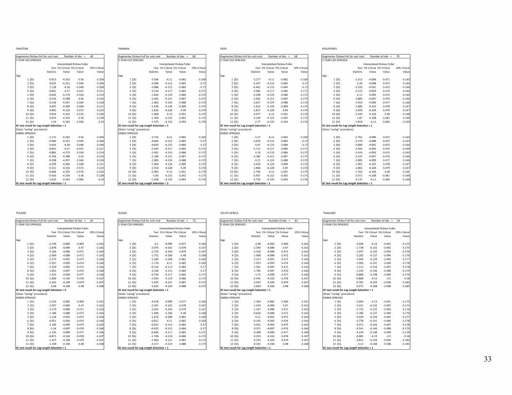
33

PAKISTAN PANAMA PERU PHILIPPINES

AugmentedDickey‐Full for unit root         Number of obs   =       40 AugmentedDickey‐Full for unit root         Number of obs   =       68 AugmentedDickey‐Full for unit root         Number of obs   =       68 AugmentedDickey‐Full for unit root         Number of obs   =       795 YEAR CDS SPREADS 5 YEAR CDS SPREADS 5 YEAR CDS SPREADS 5 YEAR CDS SPREADS

Interpolated Dickey‐Fuller Interpolated Dickey‐Fuller Interpolated Dickey‐Fuller Interpolated Dickey‐FullerTest 1% Critical 5% Critical 10% Critical Test 1% Critical 5% Critical 10% Critical Test 1% Critical 5% Critical 10% Critical Test 1% Critical 5% Critical 10% Critical

Statistic Value Value Value Statistic Value Value Value Statistic Value Value Value Statistic Value Value Valuelags lags lags lags

1 Z(t) ‐0.913 ‐4.242 ‐3.54 ‐3.204 1 Z(t) ‐3.504 ‐4.11 ‐3.482 ‐3.169 1 Z(t) ‐3.277 ‐4.11 ‐3.482 ‐3.169 1 Z(t) ‐2.315 ‐4.086 ‐3.471 ‐3.1632 Z(t) 0.025 ‐4.251 ‐3.544 ‐3.206 2 Z(t) ‐4.286 ‐4.113 ‐3.483 ‐3.17 2 Z(t) ‐4.307 ‐4.113 ‐3.483 ‐3.17 2 Z(t) ‐2.29 ‐4.088 ‐3.472 ‐3.1633 Z(t) 1.128 ‐4.26 ‐3.548 ‐3.209 3 Z(t) ‐3.888 ‐4.115 ‐3.484 ‐3.17 3 Z(t) ‐4.461 ‐4.115 ‐3.484 ‐3.17 3 Z(t) ‐2.524 ‐4.091 ‐3.473 ‐3.1644 Z(t) ‐0.601 ‐4.27 ‐3.552 ‐3.211 4 Z(t) ‐3.516 ‐4.117 ‐3.485 ‐3.171 4 Z(t) ‐3.485 ‐4.117 ‐3.485 ‐3.171 4 Z(t) ‐2.273 ‐4.093 ‐3.474 ‐3.1645 Z(t) ‐0.644 ‐4.279 ‐3.556 ‐3.214 5 Z(t) ‐1.826 ‐4.119 ‐3.486 ‐3.172 5 Z(t) ‐2.238 ‐4.119 ‐3.486 ‐3.172 5 Z(t) ‐2.11 ‐4.095 ‐3.475 ‐3.1656 Z(t) ‐0.103 ‐4.288 ‐3.56 ‐3.216 6 Z(t) ‐2.392 ‐4.121 ‐3.487 ‐3.172 6 Z(t) ‐2.562 ‐4.121 ‐3.487 ‐3.172 6 Z(t) ‐1.885 ‐4.097 ‐3.476 ‐3.1667 Z(t) ‐0.139 ‐4.297 ‐3.564 ‐3.218 7 Z(t) ‐1.963 ‐4.124 ‐3.488 ‐3.173 7 Z(t) ‐2.027 ‐4.124 ‐3.488 ‐3.173 7 Z(t) ‐1.453 ‐4.099 ‐3.477 ‐3.1668 Z(t) 0.497 ‐4.306 ‐3.568 ‐3.221 8 Z(t) ‐2.528 ‐4.126 ‐3.489 ‐3.173 8 Z(t) ‐1.622 ‐4.126 ‐3.489 ‐3.173 8 Z(t) ‐1.685 ‐4.102 ‐3.478 ‐3.1679 Z(t) 0.891 ‐4.316 ‐3.572 ‐3.223 9 Z(t) ‐1.832 ‐4.128 ‐3.49 ‐3.174 9 Z(t) ‐1.817 ‐4.128 ‐3.49 ‐3.174 9 Z(t) ‐1.659 ‐4.104 ‐3.479 ‐3.167

10 Z(t) 0.943 ‐4.325 ‐3.576 ‐3.226 10 Z(t) ‐1.668 ‐4.13 ‐3.491 ‐3.175 10 Z(t) ‐2.077 ‐4.13 ‐3.491 ‐3.175 10 Z(t) ‐1.444 ‐4.106 ‐3.48 ‐3.16811 Z(t) 0.914 ‐4.334 ‐3.58 ‐3.228 11 Z(t) ‐1.383 ‐4.132 ‐3.492 ‐3.175 11 Z(t) ‐3.194 ‐4.132 ‐3.492 ‐3.175 11 Z(t) ‐1.87 ‐4.108 ‐3.481 ‐3.16912 Z(t) 1.54 ‐4.343 ‐3.584 ‐3.23 12 Z(t) ‐1.475 ‐4.135 ‐3.493 ‐3.176 12 Z(t) ‐2.77 ‐4.135 ‐3.493 ‐3.176 12 Z(t) ‐1.818 ‐4.11 ‐3.482 ‐3.169

SC test result for Lag Length Selection = 1  SC test result for Lag Length Selection = 1 SC test result for Lag Length Selection = 1 SC test result for Lag Length Selection = 1(Stata "varlag" procedure) (Stata "varlag" procedure) (Stata "varlag" procedure) (Stata "varlag" procedure)EMBIG SPREADS EMBIG SPREADS EMBIG SPREADS

1 Z(t) ‐1.171 ‐4.242 ‐3.54 ‐3.204 1 Z(t) ‐3.733 ‐4.11 ‐3.482 ‐3.169 1 Z(t) ‐3.17 ‐4.11 ‐3.482 ‐3.169 1 Z(t) ‐2.761 ‐4.086 ‐3.471 ‐3.1632 Z(t) ‐0.906 ‐4.251 ‐3.544 ‐3.206 2 Z(t) ‐4.464 ‐4.113 ‐3.483 ‐3.17 2 Z(t) ‐3.655 ‐4.113 ‐3.483 ‐3.17 2 Z(t) ‐2.574 ‐4.088 ‐3.472 ‐3.1633 Z(t) 0.416 ‐4.26 ‐3.548 ‐3.209 3 Z(t) ‐4.835 ‐4.115 ‐3.484 ‐3.17 3 Z(t) ‐3.67 ‐4.115 ‐3.484 ‐3.17 3 Z(t) ‐2.899 ‐4.091 ‐3.473 ‐3.1644 Z(t) ‐0.601 ‐4.27 ‐3.552 ‐3.211 4 Z(t) ‐2.935 ‐4.117 ‐3.485 ‐3.171 4 Z(t) ‐2.711 ‐4.117 ‐3.485 ‐3.171 4 Z(t) ‐2.502 ‐4.093 ‐3.474 ‐3.1645 Z(t) ‐0.885 ‐4.279 ‐3.556 ‐3.214 5 Z(t) ‐2.401 ‐4.119 ‐3.486 ‐3.172 5 Z(t) ‐3.19 ‐4.119 ‐3.486 ‐3.172 5 Z(t) ‐2.424 ‐4.095 ‐3.475 ‐3.1656 Z(t) ‐0.766 ‐4.288 ‐3.56 ‐3.216 6 Z(t) ‐2.189 ‐4.121 ‐3.487 ‐3.172 6 Z(t) ‐3.184 ‐4.121 ‐3.487 ‐3.172 6 Z(t) ‐2.537 ‐4.097 ‐3.476 ‐3.1667 Z(t) ‐0.358 ‐4.297 ‐3.564 ‐3.218 7 Z(t) ‐2.065 ‐4.124 ‐3.488 ‐3.173 7 Z(t) ‐3.21 ‐4.124 ‐3.488 ‐3.173 7 Z(t) ‐2.085 ‐4.099 ‐3.477 ‐3.1668 Z(t) ‐0.299 ‐4.306 ‐3.568 ‐3.221 8 Z(t) ‐1.966 ‐4.126 ‐3.489 ‐3.173 8 Z(t) ‐2.426 ‐4.126 ‐3.489 ‐3.173 8 Z(t) ‐1.901 ‐4.102 ‐3.478 ‐3.1679 Z(t) ‐0.311 ‐4.316 ‐3.572 ‐3.223 9 Z(t) ‐2.554 ‐4.128 ‐3.49 ‐3.174 9 Z(t) ‐1.844 ‐4.128 ‐3.49 ‐3.174 9 Z(t) ‐1.861 ‐4.104 ‐3.479 ‐3.167

10 Z(t) ‐0.686 ‐4.325 ‐3.576 ‐3.226 10 Z(t) ‐2.003 ‐4.13 ‐3.491 ‐3.175 10 Z(t) ‐1.745 ‐4.13 ‐3.491 ‐3.175 10 Z(t) ‐1.763 ‐4.106 ‐3.48 ‐3.16811 Z(t) ‐0.443 ‐4.334 ‐3.58 ‐3.228 11 Z(t) ‐1.83 ‐4.132 ‐3.492 ‐3.175 11 Z(t) ‐2.937 ‐4.132 ‐3.492 ‐3.175 11 Z(t) ‐2.072 ‐4.108 ‐3.481 ‐3.16912 Z(t) ‐1.623 ‐4.343 ‐3.584 ‐3.23 12 Z(t) ‐1.638 ‐4.135 ‐3.493 ‐3.176 12 Z(t) ‐3.732 ‐4.135 ‐3.493 ‐3.176 12 Z(t) ‐2.137 ‐4.11 ‐3.482 ‐3.169

SC test result for Lag Length Selection = 1  SC test result for Lag Length Selection = 2 SC test result for Lag Length Selection = 1 SC test result for Lag Length Selection = 1

POLAND RUSSIA SOUTH AFRICA THAILAND

AugmentedDickey‐Full for unit root         Number of obs   =       81 AugmentedDickey‐Full for unit root         Number of obs   =       73 AugmentedDickey‐Full for unit root         Number of obs   =       81 AugmentedDickey‐Full for unit root         Number of obs   =      595 YEAR CDS SPREADS 5 YEAR CDS SPREADS 5 YEAR CDS SPREADS 5 YEAR CDS SPREADS

Interpolated Dickey‐Fuller Interpolated Dickey‐Fuller Interpolated Dickey‐Fuller Interpolated Dickey‐FullerTest 1% Critical 5% Critical 10% Critical Test 1% Critical 5% Critical 10% Critical Test 1% Critical 5% Critical 10% Critical Test 1% Critical 5% Critical 10% Critical

Statistic Value Value Value Statistic Value Value Value Statistic Value Value Value Statistic Value Value Valuelags lags lags lags

1 Z(t) ‐2.744 ‐4.082 ‐3.469 ‐3.161 1 Z(t) ‐4.1 ‐4.099 ‐3.477 ‐3.166 1 Z(t) ‐2.48 ‐4.082 ‐3.469 ‐3.161 1 Z(t) ‐2.028 ‐4.13 ‐3.491 ‐3.1752 Z(t) ‐2.878 ‐4.084 ‐3.47 ‐3.162 2 Z(t) ‐3.075 ‐4.102 ‐3.478 ‐3.167 2 Z(t) ‐2.593 ‐4.084 ‐3.47 ‐3.162 2 Z(t) ‐1.738 ‐4.132 ‐3.492 ‐3.1753 Z(t) ‐3.166 ‐4.086 ‐3.471 ‐3.163 3 Z(t) ‐2.724 ‐4.104 ‐3.479 ‐3.167 3 Z(t) ‐2.518 ‐4.086 ‐3.471 ‐3.163 3 Z(t) ‐1.937 ‐4.135 ‐3.493 ‐3.1764 Z(t) ‐2.669 ‐4.088 ‐3.472 ‐3.163 4 Z(t) ‐1.752 ‐4.106 ‐3.48 ‐3.168 4 Z(t) ‐1.908 ‐4.088 ‐3.472 ‐3.163 4 Z(t) ‐2.205 ‐4.137 ‐3.494 ‐3.1765 Z(t) ‐2.375 ‐4.091 ‐3.473 ‐3.164 5 Z(t) ‐1.289 ‐4.108 ‐3.481 ‐3.169 5 Z(t) ‐2.257 ‐4.091 ‐3.473 ‐3.164 5 Z(t) ‐1.949 ‐4.139 ‐3.495 ‐3.1776 Z(t) ‐2.037 ‐4.093 ‐3.474 ‐3.164 6 Z(t) ‐1.176 ‐4.11 ‐3.482 ‐3.169 6 Z(t) ‐1.923 ‐4.093 ‐3.474 ‐3.164 6 Z(t) ‐1.903 ‐4.141 ‐3.496 ‐3.1787 Z(t) ‐2.459 ‐4.095 ‐3.475 ‐3.165 7 Z(t) ‐0.116 ‐4.113 ‐3.483 ‐3.17 7 Z(t) ‐1.941 ‐4.095 ‐3.475 ‐3.165 7 Z(t) ‐1.115 ‐4.143 ‐3.497 ‐3.1788 Z(t) ‐1.853 ‐4.097 ‐3.476 ‐3.166 8 Z(t) 0.169 ‐4.115 ‐3.484 ‐3.17 8 Z(t) ‐1.785 ‐4.097 ‐3.476 ‐3.166 8 Z(t) ‐1.242 ‐4.146 ‐3.498 ‐3.1799 Z(t) ‐1.915 ‐4.099 ‐3.477 ‐3.166 9 Z(t) ‐0.749 ‐4.117 ‐3.485 ‐3.171 9 Z(t) ‐1.71 ‐4.099 ‐3.477 ‐3.166 9 Z(t) ‐0.889 ‐4.148 ‐3.499 ‐3.179

10 Z(t) ‐1.839 ‐4.102 ‐3.478 ‐3.167 10 Z(t) ‐1.924 ‐4.119 ‐3.486 ‐3.172 10 Z(t) ‐2.441 ‐4.102 ‐3.478 ‐3.167 10 Z(t) ‐0.808 ‐4.15 ‐3.5 ‐3.1811 Z(t) ‐2.101 ‐4.104 ‐3.479 ‐3.167 11 Z(t) ‐1.925 ‐4.121 ‐3.487 ‐3.172 11 Z(t) ‐1.507 ‐4.104 ‐3.479 ‐3.167 11 Z(t) ‐0.781 ‐4.159 ‐3.504 ‐3.18212 Z(t) ‐2.06 ‐4.106 ‐3.48 ‐3.168 12 Z(t) ‐2.623 ‐4.124 ‐3.488 ‐3.173 12 Z(t) ‐1.654 ‐4.106 ‐3.48 ‐3.168 12 Z(t) ‐0.271 ‐4.168 ‐3.508 ‐3.185

SC test result for Lag Length Selection = 5 SC test result for Lag Length Selection = 1 SC test result for Lag Length Selection = 1 SC test result for Lag Length Selection = 1(Stata "varlag" procedure) (Stata "varlag" procedure) (Stata "varlag" procedure) (Stata "varlag" procedure)EMBIG SPREADS EMBIG SPREADS EMBIG SPREADS EMBIG SPREADS

1 Z(t) ‐2.254 ‐4.082 ‐3.469 ‐3.161 1 Z(t) ‐4.678 ‐4.099 ‐3.477 ‐3.166 1 Z(t) ‐1.364 ‐4.082 ‐3.469 ‐3.161 1 Z(t) ‐2.604 ‐4.13 ‐3.491 ‐3.1752 Z(t) ‐2.007 ‐4.084 ‐3.47 ‐3.162 2 Z(t) ‐2.587 ‐4.102 ‐3.478 ‐3.167 2 Z(t) ‐1.419 ‐4.084 ‐3.47 ‐3.162 2 Z(t) ‐2.451 ‐4.132 ‐3.492 ‐3.1753 Z(t) ‐2.279 ‐4.086 ‐3.471 ‐3.163 3 Z(t) ‐2.054 ‐4.104 ‐3.479 ‐3.167 3 Z(t) ‐1.547 ‐4.086 ‐3.471 ‐3.163 3 Z(t) ‐2.732 ‐4.135 ‐3.493 ‐3.1764 Z(t) ‐1.186 ‐4.088 ‐3.472 ‐3.163 4 Z(t) ‐1.689 ‐4.106 ‐3.48 ‐3.168 4 Z(t) ‐0.656 ‐4.088 ‐3.472 ‐3.163 4 Z(t) ‐2.786 ‐4.137 ‐3.494 ‐3.1765 Z(t) ‐1.124 ‐4.091 ‐3.473 ‐3.164 5 Z(t) ‐1.476 ‐4.108 ‐3.481 ‐3.169 5 Z(t) ‐0.11 ‐4.091 ‐3.473 ‐3.164 5 Z(t) ‐4.559 ‐4.139 ‐3.495 ‐3.1776 Z(t) ‐0.951 ‐4.093 ‐3.474 ‐3.164 6 Z(t) ‐0.812 ‐4.11 ‐3.482 ‐3.169 6 Z(t) ‐0.101 ‐4.093 ‐3.474 ‐3.164 6 Z(t) ‐3.778 ‐4.141 ‐3.496 ‐3.1787 Z(t) ‐1.185 ‐4.095 ‐3.475 ‐3.165 7 Z(t) ‐0.651 ‐4.113 ‐3.483 ‐3.17 7 Z(t) 0.021 ‐4.095 ‐3.475 ‐3.165 7 Z(t) ‐3.971 ‐4.143 ‐3.497 ‐3.1788 Z(t) ‐1.24 ‐4.097 ‐3.476 ‐3.166 8 Z(t) ‐0.425 ‐4.115 ‐3.484 ‐3.17 8 Z(t) 0.371 ‐4.097 ‐3.476 ‐3.166 8 Z(t) ‐3.541 ‐4.146 ‐3.498 ‐3.1799 Z(t) ‐1.135 ‐4.099 ‐3.477 ‐3.166 9 Z(t) ‐0.846 ‐4.117 ‐3.485 ‐3.171 9 Z(t) 0.289 ‐4.099 ‐3.477 ‐3.166 9 Z(t) ‐4.144 ‐4.148 ‐3.499 ‐3.179

10 Z(t) ‐0.871 ‐4.102 ‐3.478 ‐3.167 10 Z(t) ‐1.746 ‐4.119 ‐3.486 ‐3.172 10 Z(t) 0.253 ‐4.102 ‐3.478 ‐3.167 10 Z(t) ‐4.081 ‐4.15 ‐3.5 ‐3.1811 Z(t) ‐1.257 ‐4.104 ‐3.479 ‐3.167 11 Z(t) ‐1.963 ‐4.121 ‐3.487 ‐3.172 11 Z(t) 0.233 ‐4.104 ‐3.479 ‐3.167 11 Z(t) ‐3.812 ‐4.159 ‐3.504 ‐3.18212 Z(t) ‐1.169 ‐4.106 ‐3.48 ‐3.168 12 Z(t) ‐3.217 ‐4.124 ‐3.488 ‐3.173 12 Z(t) ‐0.161 ‐4.106 ‐3.48 ‐3.168 12 Z(t) ‐3.12 ‐4.168 ‐3.508 ‐3.185

SC test result for Lag Length Selection = 1 SC test result for Lag Length Selection = 1 SC test result for Lag Length Selection = 1 SC test result for Lag Length Selection = 1

34

TUNISIA TURKEY UKRAINE URUGUAY

AugmentedDickey‐Full for unit root         Number of obs   =      24 AugmentedDickey‐Full for unit root         Number of obs   =      81 AugmentedDickey‐Full for unit root         Number of obs   =      51 AugmentedDickey‐Full for unit root         Number of obs   =     335 YEAR CDS SPREADS 5 YEAR CDS SPREADS 5 YEAR CDS SPREADS 5 YEAR CDS SPREADS

Interpolated Dickey‐Fuller Interpolated Dickey‐Fuller Interpolated Dickey‐Fu10% Critical Interpolated Dickey‐FullerTest 1% Critical 5% Critical 10% Critical Test 1% Critical 5% Critical 10% Critical Test 1% Critical 5% Critical Value Test 1% Critical 5% Critical 10% Critical

Statistic Value Value Value Statistic Value Value Value Statistic Value Value Statistic Value Value Valuelags lags lags lags

1 Z(t) ‐2.096 ‐4.38 ‐3.6 ‐3.24 1 Z(t) ‐3.165 ‐4.082 ‐3.469 ‐3.161 1 Z(t) ‐2.615 ‐4.148 ‐3.499 ‐3.179 1 Z(t) ‐1.437 ‐4.306 ‐3.568 ‐3.2212 Z(t) ‐2.119 ‐4.38 ‐3.6 ‐3.24 2 Z(t) ‐3.091 ‐4.084 ‐3.47 ‐3.162 2 Z(t) ‐2.723 ‐4.15 ‐3.5 ‐3.18 2 Z(t) ‐1.249 ‐4.316 ‐3.572 ‐3.2233 Z(t) ‐2.259 ‐4.38 ‐3.6 ‐3.24 3 Z(t) ‐3.237 ‐4.086 ‐3.471 ‐3.163 3 Z(t) ‐2.266 ‐4.159 ‐3.504 ‐3.182 3 Z(t) ‐1.757 ‐4.325 ‐3.576 ‐3.2264 Z(t) ‐2.936 ‐4.38 ‐3.6 ‐3.24 4 Z(t) ‐3.022 ‐4.088 ‐3.472 ‐3.163 4 Z(t) ‐3.215 ‐4.168 ‐3.508 ‐3.185 4 Z(t) ‐1.592 ‐4.334 ‐3.58 ‐3.2285 Z(t) ‐3.809 ‐4.38 ‐3.6 ‐3.24 5 Z(t) ‐2.521 ‐4.091 ‐3.473 ‐3.164 5 Z(t) ‐1.618 ‐4.178 ‐3.512 ‐3.187 5 Z(t) ‐0.975 ‐4.343 ‐3.584 ‐3.236 Z(t) ‐2.599 ‐4.38 ‐3.6 ‐3.24 6 Z(t) ‐2.061 ‐4.093 ‐3.474 ‐3.164 6 Z(t) ‐1.41 ‐4.187 ‐3.516 ‐3.19 6 Z(t) ‐0.977 ‐4.352 ‐3.588 ‐3.2337 Z(t) ‐2.244 ‐4.38 ‐3.6 ‐3.24 7 Z(t) ‐1.984 ‐4.095 ‐3.475 ‐3.165 7 Z(t) ‐1.233 ‐4.196 ‐3.52 ‐3.192 7 Z(t) ‐1.532 ‐4.362 ‐3.592 ‐3.2358 Z(t) ‐1.451 ‐4.38 ‐3.6 ‐3.24 8 Z(t) ‐1.683 ‐4.097 ‐3.476 ‐3.166 8 Z(t) ‐1.004 ‐4.205 ‐3.524 ‐3.194 8 Z(t) ‐1.813 ‐4.371 ‐3.596 ‐3.2389 Z(t) ‐1.052 ‐4.38 ‐3.6 ‐3.24 9 Z(t) ‐1.702 ‐4.099 ‐3.477 ‐3.166 9 Z(t) ‐1.125 ‐4.214 ‐3.528 ‐3.197 9 Z(t) ‐1.473 ‐4.38 ‐3.6 ‐3.24

10 Z(t) ‐2.177 ‐4.38 ‐3.6 ‐3.24 10 Z(t) ‐1.598 ‐4.102 ‐3.478 ‐3.167 10 Z(t) ‐1.122 ‐4.224 ‐3.532 ‐3.199 10 Z(t) ‐1.751 ‐4.38 ‐3.6 ‐3.2411 Z(t) 11 Z(t) ‐1.867 ‐4.104 ‐3.479 ‐3.167 11 Z(t) ‐0.959 ‐4.233 ‐3.536 ‐3.202 11 Z(t) ‐1.729 ‐4.38 ‐3.6 ‐3.2412 Z(t) 12 Z(t) ‐2.272 ‐4.106 ‐3.48 ‐3.168 12 Z(t) ‐1.277 ‐4.242 ‐3.54 ‐3.204 12 Z(t) ‐1.238 ‐4.38 ‐3.6 ‐3.24

SC test result for Lag Length Selection = 1  SC test result for Lag Length Selection = 1 SC test result for Lag Length Selection = 1 SC test result for Lag Length Selection = 1(Stata "varlag" procedure) (Stata "varlag" procedure) (Stata "varlag" procedure) (Stata "varlag" procedure)EMBIG SPREADS EMBIG SPREADS EMBIG SPREADS EMBIG SPREADS

1 Z(t) ‐1.124 ‐4.38 ‐3.6 ‐3.24 1 Z(t) ‐3.029 ‐4.082 ‐3.469 ‐3.161 1 Z(t) ‐1.086 ‐4.148 ‐3.499 ‐3.179 1 Z(t) ‐2.084 ‐4.306 ‐3.568 ‐3.2212 Z(t) ‐0.569 ‐4.38 ‐3.6 ‐3.24 2 Z(t) ‐2.611 ‐4.084 ‐3.47 ‐3.162 2 Z(t) ‐1.001 ‐4.15 ‐3.5 ‐3.18 2 Z(t) ‐1.23 ‐4.316 ‐3.572 ‐3.2233 Z(t) ‐0.926 ‐4.38 ‐3.6 ‐3.24 3 Z(t) ‐3.069 ‐4.086 ‐3.471 ‐3.163 3 Z(t) ‐0.431 ‐4.159 ‐3.504 ‐3.182 3 Z(t) ‐1.086 ‐4.325 ‐3.576 ‐3.2264 Z(t) ‐1.567 ‐4.38 ‐3.6 ‐3.24 4 Z(t) ‐2.411 ‐4.088 ‐3.472 ‐3.163 4 Z(t) ‐0.701 ‐4.168 ‐3.508 ‐3.185 4 Z(t) ‐1.176 ‐4.334 ‐3.58 ‐3.2285 Z(t) ‐1.919 ‐4.38 ‐3.6 ‐3.24 5 Z(t) ‐2.186 ‐4.091 ‐3.473 ‐3.164 5 Z(t) ‐1.301 ‐4.178 ‐3.512 ‐3.187 5 Z(t) ‐1.366 ‐4.343 ‐3.584 ‐3.236 Z(t) ‐1.434 ‐4.38 ‐3.6 ‐3.24 6 Z(t) ‐1.97 ‐4.093 ‐3.474 ‐3.164 6 Z(t) ‐1.01 ‐4.187 ‐3.516 ‐3.19 6 Z(t) ‐0.998 ‐4.352 ‐3.588 ‐3.2337 Z(t) ‐1.205 ‐4.38 ‐3.6 ‐3.24 7 Z(t) ‐1.565 ‐4.095 ‐3.475 ‐3.165 7 Z(t) ‐0.933 ‐4.196 ‐3.52 ‐3.192 7 Z(t) ‐1.592 ‐4.362 ‐3.592 ‐3.2358 Z(t) ‐0.168 ‐4.38 ‐3.6 ‐3.24 8 Z(t) ‐1.48 ‐4.097 ‐3.476 ‐3.166 8 Z(t) ‐0.802 ‐4.205 ‐3.524 ‐3.194 8 Z(t) ‐0.714 ‐4.371 ‐3.596 ‐3.2389 Z(t) ‐0.406 ‐4.38 ‐3.6 ‐3.24 9 Z(t) ‐1.275 ‐4.099 ‐3.477 ‐3.166 9 Z(t) ‐0.735 ‐4.214 ‐3.528 ‐3.197 9 Z(t) ‐1.117 ‐4.38 ‐3.6 ‐3.24

10 Z(t) ‐0.752 ‐4.38 ‐3.6 ‐3.24 10 Z(t) ‐0.921 ‐4.102 ‐3.478 ‐3.167 10 Z(t) ‐0.626 ‐4.224 ‐3.532 ‐3.199 10 Z(t) ‐1.089 ‐4.38 ‐3.6 ‐3.2411 Z(t) 11 Z(t) ‐1.189 ‐4.104 ‐3.479 ‐3.167 11 Z(t) ‐0.03 ‐4.233 ‐3.536 ‐3.202 11 Z(t) ‐1.077 ‐4.38 ‐3.6 ‐3.2412 Z(t) 12 Z(t) ‐1.409 ‐4.106 ‐3.48 ‐3.168 12 Z(t) 0.236 ‐4.242 ‐3.54 ‐3.204 12 Z(t) 0.751 ‐4.38 ‐3.6 ‐3.24

SC test result for Lag Length Selection = 1  SC test result for Lag Length Selection = 1 SC test result for Lag Length Selection = 1 SC test result for Lag Length Selection = 1

VENEZUELA VIETNAM

AugmentedDickey‐Full for unit root         Number of obs   =     80 AugmentedDickey‐Full for unit root         Number of obs   =     235 YEAR CDS SPREADS 5 YEAR CDS SPREADS

Interpolated Dickey‐Fuller Interpolated Dickey‐FullerTest 1% Critical 5% Critical 10% Critical Test 1% Critical 5% Critical 10% Critical

Statistic Value Value Value Statistic Value Value Valuelags lags

1 Z(t) ‐2.687 ‐4.084 ‐3.47 ‐3.162 1 Z(t) ‐1.678 ‐4.38 ‐3.6 ‐3.242 Z(t) ‐2.431 ‐4.086 ‐3.471 ‐3.163 2 Z(t) ‐1.051 ‐4.38 ‐3.6 ‐3.243 Z(t) ‐2.62 ‐4.088 ‐3.472 ‐3.163 3 Z(t) ‐0.631 ‐4.38 ‐3.6 ‐3.244 Z(t) ‐2.172 ‐4.091 ‐3.473 ‐3.164 4 Z(t) 0.431 ‐4.38 ‐3.6 ‐3.245 Z(t) ‐2.092 ‐4.093 ‐3.474 ‐3.164 5 Z(t) 0.616 ‐4.38 ‐3.6 ‐3.246 Z(t) ‐2.306 ‐4.095 ‐3.475 ‐3.165 6 Z(t) 0.618 ‐4.38 ‐3.6 ‐3.247 Z(t) ‐2.042 ‐4.097 ‐3.476 ‐3.166 7 Z(t) 0.266 ‐4.38 ‐3.6 ‐3.248 Z(t) ‐2.265 ‐4.099 ‐3.477 ‐3.166 8 Z(t) ‐0.039 ‐4.38 ‐3.6 ‐3.249 Z(t) ‐1.931 ‐4.102 ‐3.478 ‐3.167 9 Z(t) ‐0.315 ‐4.38 ‐3.6 ‐3.2410 Z(t) ‐1.17 ‐4.104 ‐3.479 ‐3.167 10 Z(t) ‐0.167 ‐4.38 ‐3.6 ‐3.2411 Z(t) ‐0.774 ‐4.106 ‐3.48 ‐3.168 11 Z(t)12 Z(t) ‐1.237 ‐4.108 ‐3.481 ‐3.169 12 Z(t)

SC test result for Lag Length Selection = 1 SC test result for Lag Length Selection = 1 (Stata "varlag" procedure) (Stata "varlag" procedure)EMBIG SPREADS EMBIG SPREADS

1 Z(t) ‐1.981 ‐4.084 ‐3.47 ‐3.162 1 Z(t) ‐1.464 ‐4.38 ‐3.6 ‐3.242 Z(t) ‐1.917 ‐4.086 ‐3.471 ‐3.163 2 Z(t) 0.021 ‐4.38 ‐3.6 ‐3.243 Z(t) ‐1.95 ‐4.088 ‐3.472 ‐3.163 3 Z(t) 0.526 ‐4.38 ‐3.6 ‐3.244 Z(t) ‐1.475 ‐4.091 ‐3.473 ‐3.164 4 Z(t) 0.61 ‐4.38 ‐3.6 ‐3.245 Z(t) ‐1.394 ‐4.093 ‐3.474 ‐3.164 5 Z(t) ‐0.066 ‐4.38 ‐3.6 ‐3.246 Z(t) ‐1.717 ‐4.095 ‐3.475 ‐3.165 6 Z(t) 0.086 ‐4.38 ‐3.6 ‐3.247 Z(t) ‐1.327 ‐4.097 ‐3.476 ‐3.166 7 Z(t) 0.05 ‐4.38 ‐3.6 ‐3.248 Z(t) ‐1.581 ‐4.099 ‐3.477 ‐3.166 8 Z(t) 0.624 ‐4.38 ‐3.6 ‐3.249 Z(t) ‐1.286 ‐4.102 ‐3.478 ‐3.167 9 Z(t) 1.019 ‐4.38 ‐3.6 ‐3.2410 Z(t) ‐0.716 ‐4.104 ‐3.479 ‐3.167 10 Z(t) ‐1.561 ‐4.38 ‐3.6 ‐3.2411 Z(t) ‐0.266 ‐4.106 ‐3.48 ‐3.168 11 Z(t)12 Z(t) ‐0.997 ‐4.108 ‐3.481 ‐3.169 12 Z(t)

SC test result for Lag Length Selection = 1 SC test result for Lag Length Selection = 1