Working Paper Series

This paper can be downloaded without charge from: http://www.richmondfed.org/publications/

Heterogeneous Borrowers in Quantitative Models of

Sovereign Default∗

Juan Carlos Hatchondo† Leonardo Martinez‡ Horacio Sapriza§

Federal Reserve Bank of Richmond Working Paper No. 07-01R

Abstract

We extend the model used in recent quantitative studies of sovereign default, allowingpolicymakers of different types to alternate in power. We show that a default episode maybe triggered by a change in the type of policymaker in office, and that such a default islikely to occur only if there is enough political stability and if policymakers encounter pooreconomic conditions. Under high political stability, political turnover enables the model togenerate a weaker correlation between economic conditions and default decisions, a higherand more volatile spread, and lower borrowing levels after a default episode.

JEL classification: F34, F41.

Keywords: Sovereign Default, Political Risk, Endogenous Borrowing Constraints, Markov-Perfect Equilibrium.

∗We thank two anonymous referees, our colleagues at the Federal Reserve Bank of Richmond, and seminarparticipants at the 2006 Midwest Theory Meetings, the 2006 Midwest Macroeconomics Meetings, the Institute forInternational Economic Studies at the University of Stockholm, the 2006 SED, the 2006 Federal Reserve SystemMeeting on International Economics, the 2006 Wegmans Conference, the 2007 North American Winter Meetingsof the Econometric Society, the 2008 Federal Reserve System Macroeconomics Meeting, the Universidad Nacionalde Tucuman, and the Pontificia Universidad Catolica de Chile for comments and suggestions. In particular, wethank Cristina Arellano, Marina Azzimonti Renzo, and Martin Bodenstein for helpful discussions of this paper.We also thank Elaine Mandaleris-Preddy for editorial comments. All remaining mistakes are our own. Anyopinions expressed in this paper are those of the authors and do not necessarily reflect those of the FederalReserve Bank of Richmond or the Federal Reserve System.

†Federal Reserve Bank of Richmond, e-mail: juancarlos.hatchondo@rich.frb.org.‡Federal Reserve Bank of Richmond, e-mail: leonardo.martinez@rich.frb.org.§Rutgers University, e-mail: hsapriza@andromeda.rutgers.edu.

1

1 Introduction

Business cycles in small emerging economies differ from those in developed economies. Emerging

economies feature interest rates that are higher, more volatile and countercyclical (interest rates

are usually acyclical in developed economies), and have higher output volatility, higher volatility

of consumption relative to income, and more countercyclical net exports.1 Because the interest

rate is highly volatile and countercyclical, a state-dependent interest rate schedule plays an

important role in any model designed to explain the cyclical behavior of quantities and prices in

emerging economies. Some studies assume an exogenous interest rate schedule.2 Others provide

microfoundations for this schedule based on the risk of default.3 This is the approach followed

by recent quantitative models of sovereign default, based on the framework proposed by Eaton

and Gersovitz (1981).4 The present paper introduces political turnover into the second class of

models.

In addition to pure economic variables, political factors are often considered to play a non-

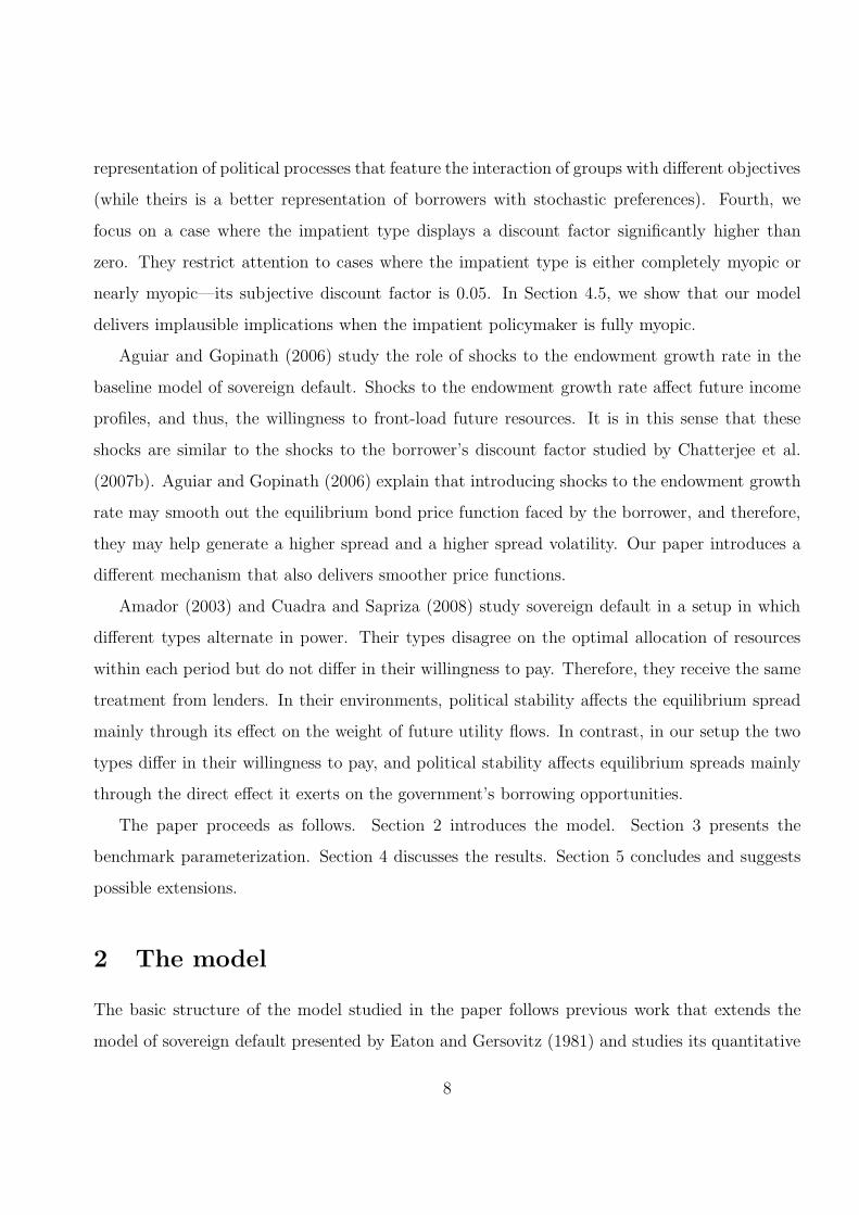
trivial role as determinants of defaults.5 Figure 1 illustrates the behavior of the sovereign spread

in Brazil before and after the 2002 election. This behavior is often mentioned as an example of

the importance of political factors as determinants of default decisions. As discussed by Goretti

(2005), the concerns raised because of left-wing candidate Luiz Inacio “Lula” Da Silva’s declara-

tions in favor of a debt repudiation is the most accepted explanation for the sharp increase in the

country spread preceding the Brazilian election. Pimentel and Murphy (2006) explain that more

recently, the elected president of Ecuador—Rafael Correa—declared his intentions to restructure

the country’s debt, which was linked to a decline in sovereign bond prices. Our paper contributes

to the understanding of how political risk may affect borrowing and default decisions.

1See, for example, Aguiar and Gopinath (2007), Neumeyer and Perri (2005), and Uribe and Yue (2006).2See, for example, Aguiar and Gopinath (2007), Neumeyer and Perri (2005), Schmitt-Grohe and Uribe (2003),

and Uribe and Yue (2006).3Tomz and Wright (2007) document 250 sovereign defaults by 106 countries between 1820 and 2004. Some of

the latest episodes are Russia in 1998, Ecuador in 1999, and Argentina in 2001.4See, for example, Aguiar and Gopinath (2006), Arellano (2008), Arellano and Ramanarayanan (2006), Bai

and Zhang (2006), Bi (2006), Cuadra and Sapriza (2006, 2008), Eyigungor (2006), Hatchondo and Martinez(2008), Hatchondo et al. (2006, 2007b), Lizarazo (2005, 2006), and Yue (2005).

5See, for example, Balkan (1992), Citron and Nickelsburg (1997), Kohlscheen (2003), Meyersson (2006), Rein-hart et al. (2003), Moser (2006), Santiso (2003), Sturzenegger and Zettelmeyer (2006), and Van Rijckeghem and

2

12/3/2001 4/26/2002 9/17/2002 2/8/2003 7/2/2003

2002 - 2003

2

7

12

17

22

Inte

rest

rat

e sp

read

(in

%)

Elections: first round

Argentinian Default

Elections: second round

Figure 1: Elections and sovereign bond spread in Brazil. Source: JP Morgan (EMBI Global)

We introduce a stylized political process into the framework used in recent quantitative studies

on sovereign default. We study a small open economy that receives a stochastic endowment

stream of a single tradable good. The objective of the policymaker in office is to maximize the

expected present value of future utility flows. As in Cole et al. (1995) and Alfaro and Kanczuk

(2005), we assume that two types of policymakers who assign different weights to future utility

flows alternate in power. One type is more patient than the other. The only financial assets

available are one-period non-contingent bonds. These assets are priced in a competitive market

inhabited by a large number of identical risk-neutral lenders. Lenders have perfect information

about the economy’s endowment and the type of policymaker in office. In each period, the

policymaker in office makes two decisions. First, he decides whether to refuse to pay previously

issued debt. Second, he decides how much to borrow or save. The cost of declaring a default is

that the endowment is reduced by a fixed percentage in the following period.

Two types of defaults may be observed in equilibrium. First, a sufficiently low endowment

realization may trigger a default during the spell of a “patient” or “impatient” type. The second

type is a “political default,” which is triggered by a change in the policymaker in power. We find

Weder (2004).

3

that in equilibrium, a political default may only occur when a patient policymaker is replaced

by an impatient policymaker.

We show that a political default is likely to occur only when there is enough political stability.

The intuition behind the role of political stability is the following. The price received by the

government for the bonds issued today incorporates a discount that mirrors the probability of a

default in the following period (recall that the government can only issue one-period bonds). If a

patient type chooses borrowing levels that would lead an impatient type to default next period,

it has to compensate lenders for this contingency, i.e., for the contingency that an impatient type

becomes the decision maker in the following period. If the probability of this contingency is high

enough (political stability is low), it is too expensive for the patient type to choose borrowing

levels that would lead an impatient type to default. In this scenario, the patient type does not

borrow so heavily and, therefore, a change in the government’s type does not trigger a default.

It is shown that our model displays a non-monotonic relationship between the default prob-

ability and political stability. On the one hand, for low levels of political stability (i.e., a high

probability of change in the type in power), an increase in political stability increases the prob-

ability that a patient government chooses debt levels that would lead an impatient government

to default and, therefore, it increases the default probability. On the other hand, for high levels

of political stability, a patient government is already choosing debt levels that would lead an

impatient government to default. In this case, the default risk premia charged on current bond

issuances already incorporate the probability that the type in power may change tomorrow.

Therefore, a decrease in that probability (i.e., more political stability) decreases the probability

of default.

We find that even in an economy with high political stability, a default does not occur every

time a patient policymaker is replaced by an impatient policymaker. The reason is that a patient

policymaker chooses high issuance volumes (that would lead an impatient policymaker to default)

only after experiencing a stream of sufficiently low endowment realizations during his tenure.

Furthermore, we show that the occurrence of political defaults enables the model to partially

disentangle default decisions from poor economic conditions. Tomz and Wright (2007) report

that even though most default episodes occur in periods of low output (below the trend), the

4

correlation between default decisions and economic conditions is much weaker than that implied

by existing quantitative models of sovereign default (without political turnover). They conjecture

that introducing “political shocks” to the model may help explain the moderate correlation

between output and default decisions found in the data. Our results support their conjecture.

In addition, we find that a distinctive feature of political defaults is that post-default debt

levels are lower than pre-default levels. The observed difficulties in market access after a default

episode—for example, Gelos et al. (2004) and IMF (2002) discuss evidence of a drainage in capital

flows to countries that defaulted—has been used in recent quantitative work on sovereign default

to motivate the assumption that countries are exogenously excluded from capital markets after

a default. In this paper, we do not assume that a defaulting country is exogenously excluded

from capital markets. However, we show that difficulties in market access after a political default

may be triggered by the political turnover that preceded the default. Recall that in our model,

a political default occurs because a patient government is replaced by an impatient one. After a

political default, investors are still willing to lend to the post-default (impatient) government but

under more stringent conditions: The bond price schedule offered to the post-default government

is below that offered to the pre-default (patient) government. We show that this induces impa-

tient post-default governments to choose debt levels that are lower than the pre-default levels.

Furthermore, and consistent with historical evidence, our model predicts that in the periods that

follow a political default, market access improves after the defaulting government loses power.6

On the contrary, if a default is non-political, the model does not predict significant differences

between post-default and pre-default debt levels. Without political turnover, in general, there is

no reason why the optimal debt level chosen by the post-default government should be signifi-

cantly different from the pre-default levels. We show that post-default debt levels quickly come

back to pre-default levels after a non-political default.

Our simulations show that introducing political turnover improves the ability of the model

to reproduce the high spread (margin of extra yield over U.S. Treasury bonds) paid by emerging

6A clear example is discussed by Cole et al. (1995): They explain that “the ability of Reconstruction govern-ments in Florida and Mississippi to borrow after the Civil War suggests that the old creditors could not blocknew loans once the states’ reputations had been restored by an observable change in regime.”

5

economies. The average spread observed in the politically stable economy is 6.3%. This spread

level is substantially higher than that obtained when political turnover is shut down. In an

economy where all policymakers are patient, the average spread is 0.3%. In an economy where

all policymakers are impatient, the average spread is 1.5%. Given that the mean spread in the

model mirrors the default probability, the previous finding implies that an economy in which

investor-friendly governments alternate in power with less investor-friendly governments displays

a higher default probability than an economy in which governments are never friendly to investors.

It is the alternation in power of different types of policymakers that is crucial for generating a

higher default probability.

It is also shown that the presence of political turnover narrows the gap between the spread

volatility generated by the model and the spread volatility observed in the data. The model

with political turnover and high political stability generates a standard deviation of the spread

of 0.42%. It should be stressed that this measure of spread volatility derives from samples where

only the patient type is in office, and therefore, it is not trivially driven by having two different

policymakers willing to accept different spread levels. The standard deviation obtained when

the model is simulated without political turnover is less than 0.03%. Thus, introducing political

turnover narrows the gap between the spread volatility in the model and the one in the data.7

Mechanically, the presence of political turnover smoothes out the bond price schedule faced by

the government. This helps the model generate a higher and more volatile spread. The shape of

the bond price function plays a key role in the quantitative performance of models of sovereign

default—see, for example, the discussions in Aguiar and Gopinath (2006) and Hatchondo et al.

(2007b). In addition to improving the spread behavior in the simulations, the model with political

turnover is able to replicate other salient features of the macroeconomic performance of emerging

economies.

7Emerging economies feature relatively high spread volatility. For instance, the standard deviation of thespread in Argentina between 1993 and 2001 equals 2.51%.

6

1.1 Related literature

This paper is closely related to Cole et al. (1995) and Alfaro and Kanczuk (2005). They study

models of sovereign default with heterogeneous borrowers in which a default occurs if a “pa-

tient” policymaker is replaced by an “impatient” policymaker. In contrast to the present paper,

they assume that there is asymmetric information about the government’s type. In order to

simplify the lenders’ learning process and make their models tractable, these studies limit the

government’s ability to choose its borrowing level. The drawback of this approach is that it is

less suitable to study macroeconomic behavior over the business cycle. These papers also focus

on equilibria in which patient policymakers never default and impatient policymakers always

default. We consider a political process similar to the one used by Cole et al. (1995) and Alfaro

and Kanczuk (2005), but ours is embedded in the setup used in recent quantitative models of

sovereign default. This means that the government does not face any restriction when choosing

the optimal borrowing level. We show that a default is likely to be triggered by political turnover

only if there is enough political stability and patient governments encounter poor economic con-

ditions during their tenure. We also show that in politically stable economies, the presence of

political turnover increases the volatility of the spread paid by patient governments.

The models used in recent quantitative studies of sovereign default share blueprints with the

models used in quantitative studies of household bankruptcy—see, for example, Athreya (2002),

Chatterjee et al. (2007a), Chatterjee et al. (2007b), Li and Sarte (2006), and Livshits et al. (2007).

Within the second literature, Chatterjee et al. (2007b) is the study that is most closely related

to this paper. They too analyze a setup with heterogenous borrowers, but our model differs from

theirs in several dimensions. First, we assume that the type of policymaker in power is public

information. They assume that lenders cannot directly observe a borrower’s type. Second, we

allow policymakers to choose debt levels from a continuum. As in Cole et al. (1995) and Alfaro

and Kanczuk (2005), they restrict the set of savings levels available to borrowers to a discrete

and coarse grid (with only three possible asset positions). Third, we assume that borrowers of

different types alternate in power. They assume that the borrower’s discount factor follows a

stochastic process, i.e., the borrower’s type changes over time. We consider ours to be a better

7

representation of political processes that feature the interaction of groups with different objectives

(while theirs is a better representation of borrowers with stochastic preferences). Fourth, we

focus on a case where the impatient type displays a discount factor significantly higher than

zero. They restrict attention to cases where the impatient type is either completely myopic or

nearly myopic—its subjective discount factor is 0.05. In Section 4.5, we show that our model

delivers implausible implications when the impatient policymaker is fully myopic.

Aguiar and Gopinath (2006) study the role of shocks to the endowment growth rate in the

baseline model of sovereign default. Shocks to the endowment growth rate affect future income

profiles, and thus, the willingness to front-load future resources. It is in this sense that these

shocks are similar to the shocks to the borrower’s discount factor studied by Chatterjee et al.

(2007b). Aguiar and Gopinath (2006) explain that introducing shocks to the endowment growth

rate may smooth out the equilibrium bond price function faced by the borrower, and therefore,

they may help generate a higher spread and a higher spread volatility. Our paper introduces a

different mechanism that also delivers smoother price functions.

Amador (2003) and Cuadra and Sapriza (2008) study sovereign default in a setup in which

different types alternate in power. Their types disagree on the optimal allocation of resources

within each period but do not differ in their willingness to pay. Therefore, they receive the same

treatment from lenders. In their environments, political stability affects the equilibrium spread

mainly through its effect on the weight of future utility flows. In contrast, in our setup the two

types differ in their willingness to pay, and political stability affects equilibrium spreads mainly

through the direct effect it exerts on the government’s borrowing opportunities.

The paper proceeds as follows. Section 2 introduces the model. Section 3 presents the

benchmark parameterization. Section 4 discusses the results. Section 5 concludes and suggests

possible extensions.

2 The model

The basic structure of the model studied in the paper follows previous work that extends the

model of sovereign default presented by Eaton and Gersovitz (1981) and studies its quantitative

8

performance. Among these studies, the closest reference to the present paper is Aguiar and

Gopinath (2006). The advantage of their model is that its simplicity allows us to analyze the

effects of political factors more transparently.

2.1 The environment

There is a single tradable good. The economy receives a stochastic endowment stream of y,

where

log(yt) = (1 − ρ) µ + ρ log(yt−1) + εt, (1)

|ρ| < 1, and εt ∼ N (0, σ2

ǫ ).

The government determines the consumption level in the economy, c. The per-period utility

function is of the CRRA type, i.e.,

u (c) =c1−σ − 1

1 − σ.

The objective of the policymaker in power is to maximize the present discounted value of future

utility flows. As in Cole et al. (1995) and Alfaro and Kanczuk (2005), we assume that two types

of policymakers who assign different weights to future utility flows alternate in power. Patient

policymakers discount future utility flows at a rate βH . Impatient policymakers discount future

utility flows at a rate βL, where βH > βL. At the end of every period, the type of policymaker in

power changes with probability π. The value of π is not state dependent. This simple political

process has the advantage of making our model a parsimonious generalization of the framework

used in recent quantitative studies and, thus, helps gauge the role played by the new mechanism

introduced in this paper.

The policymaker in power makes two decisions every period. First, he decides whether to pay

back previously issued debt. Second, he chooses how much to borrow or save for the following

period. Defaults imply a total repudiation of government debt. The only financial assets available

are one-period non-contingent bonds. Let b denote the bond position at the beginning of the

period. A negative value of b denotes that the country was an issuer of bonds in the previous

period. Each bond delivers one unit of the good in the next period (provided a default is not

9

declared). The cost of declaring a default is that the endowment in the following period is

reduced by a fraction λ.

There is a continuum of risk-neutral lenders. Each lender can borrow or lend at the risk-

free rate r. Lenders have perfect information regarding the economy’s endowment and the

government’s type.

The equilibrium bond price is determined as follows. First, the government announces how

many bonds it wants to issue. Second, lenders offer a price for the bonds. Finally, the government

sells bonds to the lenders who offered the highest price. Let qjd (b′, y) denote the equilibrium

price offered for each bond when the government issues a total of −b′ bonds. The subindex

j ∈ {H, L} indicates the government’s type. The subindex d is equal to 1 if the government

has defaulted in the current period and is equal to 0 if it has not. The price qjd (b′, y) does not

depend on default decisions in previous periods because we assume that the effect of a default

on output only lasts for one period and lenders are forward looking.

The following equation summarizes the government’s budget constraint in a given period:

c + qjd (b′, y) b′ = (1 − hλ) y + (1 − d) b,

where h denotes the credit history. The variable h takes a value of 1 if a default was declared in

the previous period and takes a value of 0 otherwise.

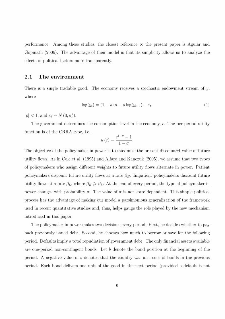
The timing in the model is summarized in Figure 2. At the beginning of the period, there

is a type-j policymaker in power. He observes the endowment realization and decides whether

to pay back previously issued debt. If the decision is to pay back, the policymaker issues an

amount −b′j0 (bt, yt, ht) of bonds. If the decision is to default, the policymaker issues an amount

−b′j1 (yt, ht) of bonds. Before the beginning of period t + 1, the type of policymaker in power

changes with probability π and does not change with probability 1 − π. In the period following

a default, the economy suffers an output loss of λ percent.

When deciding whether to default, the policymaker in power compares two continuation

values, Vj1 (y, h) and Vj0 (b, y, h). The former denotes the value function of a policymaker of

type j if a default is declared in the current period, the current endowment realization is y, and

the credit history is h. The second expression denotes the value function of a policymaker of

10

t

β j is inpower

yt is realized

Pay backbt

Default onbt

Issueb’j0(bt , yt , ht)

Issueb’j1(yt , ht)

Type j is replaced

Type j continues

Type j is replaced

Type j continues

t +1

t +1

t +1

t +1

Output loss

of λ %

Figure 2: Order of events in period t.

type j if a default is not declared in the current period, the current endowment realization is y,

and the credit history is h.

Let Vj(b, y, h) denote the value function of a policymaker of type j at the beginning of a

period when he is in power. Let Wj(b, y, h) denote the value function of a policymaker of type j

at the beginning of a period when he is not in power. Since the behavior of the two types may

differ, the value functions Vj and Wj do not need to coincide. The optimal borrowing decision of

a government that has defaulted in the current period solves the following dynamic programming

problem:

Vj1 (y, h) = maxb′

u (y (1 − hλ) − qj1 (b′, y) b′)+

βj

[

π∫

Wj(b′, y′, 1)F (dy′ | y) + (1 − π)

∫

Vj(b′, y′, 1)F (dy′ | y)

]

, (2)

where F (·) denotes the cumulative distribution function for y′. The value function of a policy-

maker of type j when he has decided to pay back its debt is obtained from the following Bellman

equation:

11

Vj0 (b, y, h) = maxb′

u (y (1 − hλ) + b − qj0 (b′, y) b′) +

βj

[

π∫

Wj(b′, y′, 0)F (dy′ | y) + (1 − π)

∫

Vj(b′, y′, 0)F (dy′ | y)

]

. (3)

The function Vj (b, y, h) is computed as follows:

Vj (b, y, h) = max{Vj1 (y, h) , Vj0 (b, y, h)}. (4)

Let dj (b, y, h) denote the optimal default decision of a policymaker of type j, namely,

dj (b, y, h) =

1 if Vj1 (y, h) > Vj0 (b, y, h)

0 if Vj1 (y, h) ≤ Vj0 (b, y, h) .(5)

The value function of a policymaker of type j when he is not in office depends on the optimal

behavior of the other type, denoted by −j. In the set of states where type −j finds it optimal to

default (d−j (b, y, h) = 1), the value function of a policymaker of type j when he is not in office

is given by

Wj (b, y, h) = u(

y (1 − hλ) − q−j1

(

b′−j1 (y, h) , y

)

b′−j1 (y, h)

)

+ (6)

βj

[

π∫

Vj(b′

−j1 (y, h) , y′, 1)F (dy′ | y) + (1 − π)∫

Wj(b′

−j1 (y, h) , y′, 1)F (dy′ | y)]

,

where b′−j1 (y, h) denotes the optimal saving behavior of a policymaker of type −j if a default has

been declared in the current period. Similarly, when type −j is in power and finds it optimal to

pay back previously issued debt (when states are such that d−j (b, y, h) = 0), the value function

of a policymaker of type j is given by

Wj (b, y, h) = u(

y (1 − hλ) + b − q−j0

(

b′−j0 (b, y, h) , y

)

b′−j0 (b, y, h)

)

+ (7)

βj

[

π∫

Vj(b′

−j0 (b, y, h) , y′, 0)F (dy′ | y) + (1 − π)∫

Wj(b′

−j0 (b, y, h) , y′, 0)F (dy′ | y)]

,

where b′−j0 (b, y, h) denotes the optimal savings of a policymaker of type −j in a period where a

default is not declared.

Bond prices satisfy the lenders’ zero profit condition. That is, bond prices are given by

12

qjd (b′, y) =1

1 + r

[

1 − π

∫

d−j (b′, y′, h′) F (dy′ | y) − (1 − π)

∫

dj (b′, y′, h′)F (dy′ | y)

]

. (8)

Bond prices depend on the credit history that the future government will inherit (h′), which

is determined by the default decision in the current period (d). Recall that defaulting in the

current period decreases future output and, therefore, affects future default decisions. Prices also

depend on the type of policymaker in power because the latter conveys information about the

probability distribution over future types and, therefore, it affects the probability distribution

over next-period default decisions.

2.2 Equilibrium Concept

We focus on differentiable Markov-perfect equilibria. Krusell and Smith (2003) show that, typ-

ically, there is a problem of indeterminacy of Markov-perfect equilibria in an infinite-horizon

economy. In order to avoid this problem, we analyze the equilibrium that arises as the limit of

the finite-horizon economy equilibrium.

Definition 1 A Markov-perfect equilibrium is characterized by

1. a set of value functions Vj (b, y, h), Vj1 (y, h), Vj0 (b, y, h), and Wj (b, y, h) for j = L, H ,

2. a set of savings rules b′j0 (b, y, h) and b′j1 (y, h), and a default decision rule dj (b, y, h) for

j = L, H ,

3. and a bond price function qjd (b′, y) for j = L, H ,

such that

(a) Vj (b, y, h), Vj1 (y, h), Vj0 (b, y, h), and Wj (b, y, h) satisfy the system of functional equations

(2)-(8);

(b) the default policy dj (b, y, h) and the savings rules b′j0 (b, y, h) and b′j1 (y, h) solve the

dynamic programming problem specified by equations (2)-(8);

(c) the bond price function qjd (b′, y) satisfies the lenders’ zero profit condition implicit in

equation (8).

13

2.3 Comparison with existing models

The environment presented above departs from the baseline model of sovereign default used in

recent quantitative studies in three dimensions. First, we do not assume that countries can be

exogenously excluded from capital markets after a default episode.8 The observed difficulties in

market access after a default episode has been used by most recent quantitative work on sovereign

default to motivate the assumption that countries are exogenously excluded from capital markets

after a default. However, the exogenous exclusion assumption is controversial on several grounds.

First, it appears to be at odds with the existence of competitive international capital markets

(assumed in this type of model). Wright (2005) discusses how in the past three decades, the

sovereign debt market has become more competitive and explains how an increase in compe-

tition (number of creditors) may diminish the creditors’ ability to coordinate; see also Wright

(2002).9 Second, empirical studies suggest that once variables such as the quality of policies and

institutions are used as controls, market access is not significantly influenced by previous default

decisions; see, for example, Eichengreen and Portes (2000), Gelos et al. (2004), and Meyersson

(2006). This suggests that it may very well be that difficulties in market access observed after

a default episode respond to the same factors that triggered the default decision itself. In this

paper, defaults and difficulties in market access that follow a default can be jointly explained by

political turnover.

The second difference between our model and previous studies is that in this paper the

output loss triggered by a default is realized in the period after the default, whereas in previous

studies the output loss lasts for a stochastic number of periods. Our assumption is motivated by

tractability reasons. Hatchondo et al. (2007b) explain that the assumption that the output loss

only takes place in one period allows us to abandon the exclusion assumption without increasing

the dimensionality of the state space. In addition, Hatchondo et al. (2007b) show that the

predictions of the model with exclusion are not affected by whether the output loss occurs in

the period after the default or for a stochastic number of periods. The output-loss assumption

8Hatchondo et al. (2007b) show that the model delivers a slightly higher equilibrium default probability withoutexclusion.

9Athreya and Janicki (2006) and Cole et al. (1995) raise a similar point.

14

intends to capture the disruptions in economic activity caused by a default decision. It has

been argued that a government default decreases private financing and, thus, it reduces output.

Using micro-level data, Arteta and Hale (2008) find that sovereign debt crises are systematically

accompanied by a large decline in foreign credit to domestic private firms. This may be the

case because a sovereign default may signal to investors a higher risk of expropriation or bad

economic conditions, and therefore, it may reduce firms’ net worth and their ability to borrow;

see Sandleris (2006) and the references therein. IMF (2002), Kumhof (2004), and Kumhof and

Tanner (2005) discuss how financial crises that lead to severe recessions follow sovereign defaults.

Similarly, Kaminsky and Reinhart (1999) show that debt devaluations in developing countries

tend to cause banking problems. Kobayashi (2006) presents a model in which a shock that

disturbs the payments system causes a decrease in aggregate productivity. Mendoza and Yue

(2007) study the link between default risk and output.

Finally, and more importantly, we allow for the possibility that the composition of the govern-

ment or the distribution of power among government officials changes over time. This possibility

is embedded in the assumption that policymakers with different time preferences alternate in

power. It should be stressed that the change of the type in power does not need to be caused

by an election. For instance, as discussed by Moser (2006) and Santiso (2003), the turnover of

finance ministers is often linked to changes in desired policies.

3 Parameterization

The model is solved numerically using value function iteration and interpolation.10 Table 1

presents the parameter values of our benchmark parameterization. We assume a coefficient of

relative risk aversion of 2. A period in the model refers to a quarter. The risk-free interest

rate is set equal to 1%. The parameter values that govern the endowment process are chosen

so as to mimic the behavior of GDP in Argentina from the fourth quarter of 1993 to the third

10The model is solved using Chebychev collocation. The algorithm finds four value functions, conditional onthe type being in office or not, and conditional on a default having been declared today or not. We use 15polynomials on the asset space and 10 on the endowment level. The results do not change significantly whenmore polynomials are used. We also verified that the conclusions presented in the paper are not altered when wesolve the model using discrete state space.

15

Risk aversion σ 2

Interest rate r 1%

Output autocorrelation coefficient ρ 0.9

Standard deviation of innovations σǫ 2.7%

Mean log output µ (-1/2)σ2

ǫ

Output loss λ 8.3%

Higher discount factor βH 0.9

Lower discount factor βL 0.6

Table 1: Parameter values.

quarter of 2001. In Section 4.4, we compare our simulation results with macroeconomic data

from Argentina during this period. The parameterization of the output process would essentially

not change if a longer sample period were considered. Aguiar and Gopinath (2006) use a similar

parameterization of the endowment process to mimic the behavior of GDP in Argentina between

1983 and 2000.

The value of λ is taken from Hatchondo et al. (2007b). When λ = 8.3%, the present value

of the cost of defaulting is similar to the cost implied by the process of output loss assumed in

Aguiar and Gopinath (2006) (a loss of 2% per period for an average duration of 10 periods).

As in previous studies, high impatience is necessary to generate default in equilibrium. For

instance, Aguiar and Gopinath (2006) choose a discount factor of 0.8. Here, we choose a higher

discount factor for the patient policymaker and a lower discount factor for the impatient policy-

maker.11

11The difference between the two discount factors could be calibrated to match differences in the actionsof different types of government. For instance, as explained in Section 4, the differences between the averageborrowing level chosen by patient and impatient governments in the model is a direct consequence of the assumeddifference between discount factors. However, the presence of other factors that affect debt levels makes it difficultto identify the extent to which differences in debt levels result from differences in political circumstances. Forexample, differences in debt levels chosen by Argentina before and after its default are not only explained bydifferences in political factors but also by the large devaluation that occurred in Argentina, as well as by changesin other economic conditions. Section 4.5 discusses how our results depend on the assumed difference betweenthe two discount factors.

16

The degree of political stability is left as a free parameter. We consider two economies that

are identical except for the degree of political stability. In the “stable” economy, the probability

that the current government type is replaced (π) is set equal to 1.5%. This implies an average

tenure in office of 16 years independently of the type. In the “unstable” economy, the value of π

is set equal to 2.5%. The latter implies an average tenure in office of 10 years. We also compare

the equilibrium in these economies with the equilibrium in economies without political turnover.

4 Results

We show that political defaults may occur in equilibrium and are likely to occur only if there is

enough political stability and if patient policymakers encounter poor economic conditions during

their tenure. Furthermore, it is shown that when the degree of political stability is high, the

presence of political turnover enables the model to generate (i) the moderate correlation between

economic conditions and default decisions documented by Tomz and Wright (2007), (ii) lower

borrowing levels after a default episode, and (iii) a higher and more volatile spread, even when

we focus on samples in which only the patient type is in office.

4.1 Political risk, default risk, and political stability

Can changes in political circumstances trigger sovereign defaults? Cole et al. (1995) and Alfaro

and Kanczuk (2005) present models in which this is the case. We add to their insight by showing

that a sovereign default is likely to be triggered by political turnover only if there is enough

political stability in the economy. Furthermore, even in an economy with high political stability,

a political default occurs only when patient policymakers encounter sufficiently poor economic

conditions during their tenure.

In order to explain how political stability may affect the relationship between political risk

and default risk, we solve the model using the parameterization in Table 1.12 We simulate the

12Bilson et al. (2002) define political risk as “the risk that arises from the potential actions of governments andother influential domestic forces, which threaten expected returns on investment.” In our environment, default isthe government’s action that affects the return obtained by lenders and, for a given debt level, political risk islow (high) when a patient (impatient) policymaker is in power.

17

model for 750,000 periods (500 samples of 1,500 observations each).

We find that in the economy with high political stability (π = 1.5%), 96% of the changes

from a patient to an impatient government trigger a default. The remaining 4% correspond to

situations in which patient governments do not encounter poor economic conditions during their

tenure. The result is different in the unstable economy. When π = 2.5%, a change in type from

βH to βL triggers a default only 4% of the time.

In what follows, we explain the link between the degree of political stability and the frequency

with which political defaults occur in equilibrium. We show that in a politically stable economy

it is more likely that a patient policymaker chooses debt levels that would lead an impatient

policymaker to default. First, we explain that impatient policymakers choose to default on lower

debt levels than do patient policymakers (Figures 3 and 4). Second, we show how differences in

the default rules of the two types and the presence of political turnover affect the bond price menu

faced by patient policymakers (Figure 5). Third, we show how the shape of the objective function

of the patient policymaker depends on the bond price menu, which helps in understanding how

the degree of political stability affects the optimal borrowing decision of a patient type (Figure 6).

We illustrate how a patient policymaker may find it optimal to choose debt levels that can trigger

a political default in the politically stable economy, but may find those debt levels suboptimal in

the politically unstable economy. Finally, we show that the patient type only chooses a borrowing

level that would lead an impatient type to default if the endowment realization is sufficiently low

(Figure 7).

In order to illustrate the mechanics of the model using two-dimensional charts, it is necessary

to hold the values of some variables fixed. For that reason, Figures 3-7 rely on specific assumptions

about the current default decision, the previous period default decision, the current endowment

level, and/or the debt level at the beginning of the period. The behavior described in the figures

would not be substantially different under alternative assumptions about those variables.

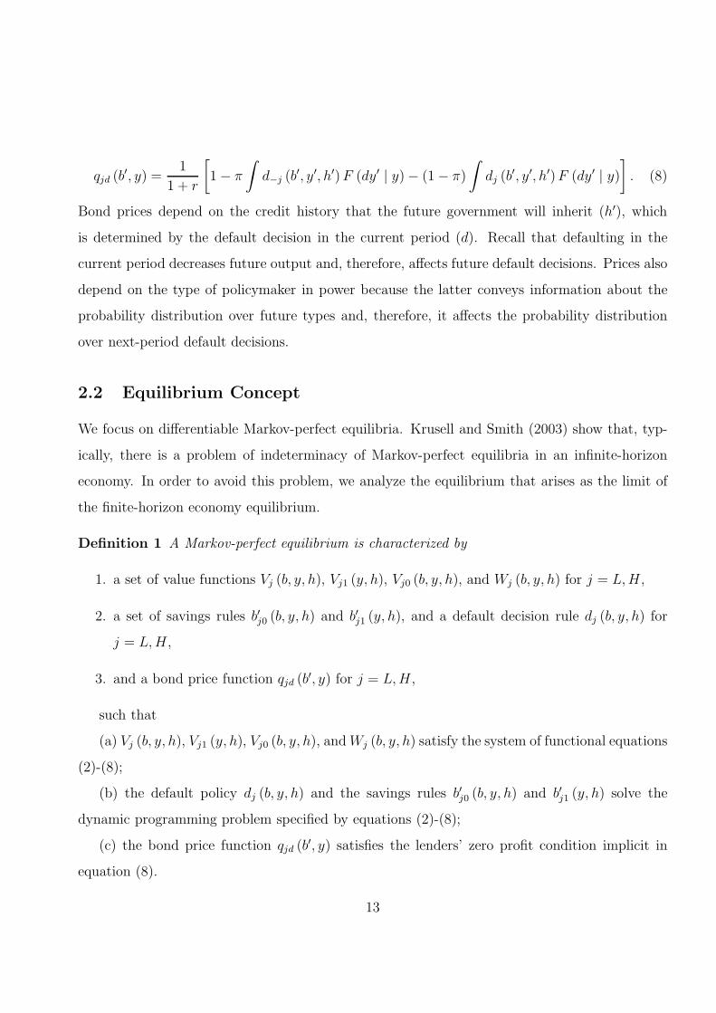
We first show that there are combinations of debt levels and endowment realizations at which

an impatient type defaults and a patient type does not default. Furthermore, for combinations of

debt levels and endowment realizations such that a patient government would choose to default,

an impatient government would also choose to default. Figure 3 shows the value functions of

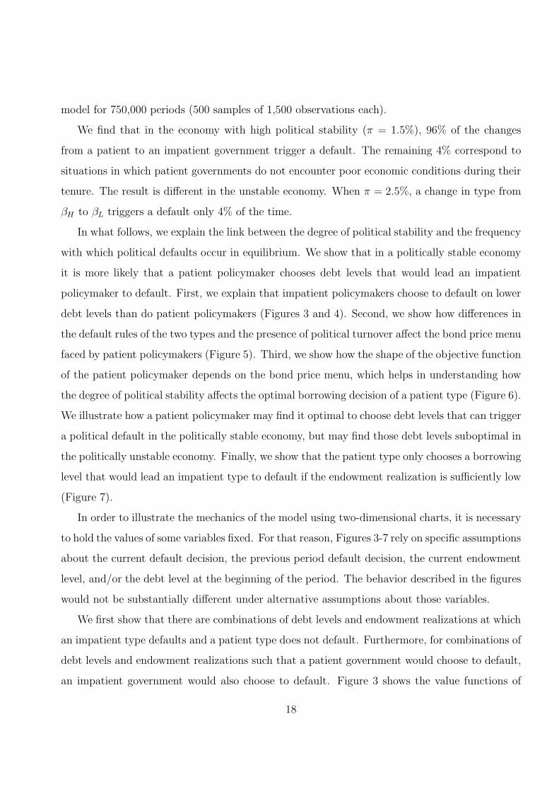
18

patient and impatient policymakers when they have defaulted and when they have not defaulted.

The value functions under default do not depend on b because a default resets the value of initial

debt to zero. The increasing curves illustrate that the expected utility of both policymakers

decreases with debt when they do not default. The scales of the left and right vertical axes of

Figure 3 were chosen so that the lines describing the value function under default of the two types

overlap. The fact that the line describing the value function under no default of a patient type

lies above the line describing the value function under no default of an impatient type implies

that there are debt levels (between 0.058 and 0.079) at which an impatient type defaults and a

patient type does not default. This is also illustrated in Figure 4, which describes the optimal

default decision of both types of policymakers.

−0.12 −0.1 −0.08 −0.06 −0.04 −0.02 0

−2.6

−2.5

b

Val

ue fu

nctio

ns fo

r β =

0.6

−0.12 −0.1 −0.08 −0.06 −0.04 −0.02 0

−10.1

−10

Val

ue fu

nctio

ns fo

r β =

0.9

No default, β = 0.6Default, β = 0.6

No default, β = 0.9Default, β = 0.9

Figure 3: Value functions in a stable economy. The figure corresponds to the case where the governmentinherits a good credit history (h = 0), and the endowment realization coincides with the unconditionalmean of the distribution.

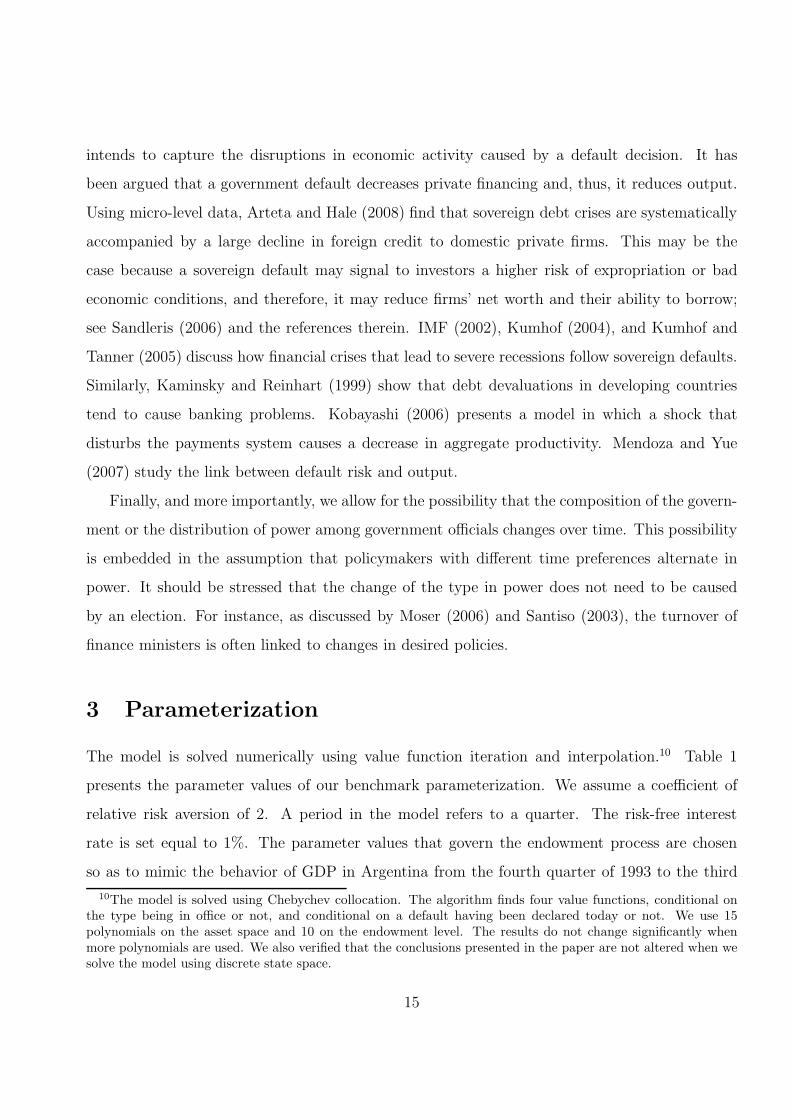
The optimal default strategies affect the shape of the bond price function faced by the pol-

icymaker in office. Figure 5 describes how the bond price menu faced by a patient type differs

across different economies: the politically stable economy, the politically unstable economy, and

the economy without political turnover. The price received by the government for the bonds

issued today incorporates a discount that mirrors the probability of a default in the following

19

−0.12 −0.1 −0.08 −0.06 −0.04 −0.02 0

0.85

0.9

0.95

1

1.05

1.1

1.15

1.2

Bond position

Out

put

Figure 4: Default regions in a stable economy. The graph corresponds to the case where the governmentinherits a good credit history (h = 0). The dark area shows combinations of bond positions andendowment realizations at which an impatient type defaults and a patient type does not default. Thegray area shows combinations of bond positions and endowment realizations at which both types default.The white area shows combinations of bond positions and endowment realizations at which neither thepatient nor the impatient type defaults.

period. This explains why the price functions in economies with political turnover display three

steps. The first step corresponds to “low” issuance volumes. At these volumes, the debt issued

is sufficiently low that the government will almost surely pay it back in the following period,

regardless of the type in power. When the issuance level is within this range of values, investors

charge the risk-free rate (bond prices are high). The second step corresponds to “intermediate”

issuance levels. In this range of issuance values, the debt issued is such that an impatient pol-

icymaker would default in the next period if he becomes the decision maker, while a patient

policymaker would pay the debt back if he remains in office. For these issuance volumes, the

default premia (spread) charged by lenders coincides with the probability of a change in the gov-

ernment type. Finally, the third step corresponds to “high” issuance volumes. At these volumes,

investors realize that the government will almost surely default tomorrow, regardless of the type

in power. Therefore, they offer a zero price for the bonds issued today (this cannot be seen in

Figure 5 because of the scale of the vertical axis).

20

Figure 5 shows that the higher the degree of political stability (i.e., the lower π), the better

the price at which a patient government can issue “intermediate” borrowing levels. As explained

above, when a patient type chooses these borrowing levels, he compensates lenders for the con-

tingency that an impatient type (who would default on “intermediate” debt levels) becomes the

decision maker in the following period. Thus, if the probability of this contingency decreases

(i.e., if π becomes lower), bond prices at “intermediate” borrowing levels increase. In addition,

Figure 5 shows that in the economy in which there is no alternation in power and all governments

are patient, the bond price menu does not feature the intermediate step.

−0.08 −0.075 −0.07 −0.065 −0.06 −0.055 −0.05 −0.045 −0.040.95

0.955

0.96

0.965

0.97

0.975

0.98

0.985

0.99

0.995

1

b’

Bon

d pr

ice

1 − π

1 + r

1

1 + r

1 − π

1 + r

−0.08 −0.075 −0.07 −0.065 −0.06 −0.055 −0.05 −0.045 −0.04

π = 1.5%

π = 2.5%No turnover

Figure 5: Bond price faced by a patient policymaker in the economies with high and low political stabil-ity and in economies without political turnover. The figure considers the case in which the endowmentrealization coincides with the unconditional mean of the distribution and in which the government hasnot defaulted today.

The shape of the government’s objective function is closely related to the shape of the bond

price function. Figure 6 shows the objective function of a patient policymaker as a function of

the current issuance volume. Typically, the objective function is not globally concave.13 For

“low” borrowing levels, the objective function is increasing with respect to the issuance volume

(−b′). For issuance values in the transition from the first to the second step of the bond price

13We use a nonlinear optimization routine to find the optimal borrowing level. The initial guess is found usinga global search procedure.

21

function, the objective function decreases with the issuance level. This accounts for the right local

maximum. Once the second step of the bond price function is reached, the objective function

becomes increasing again. Finally, as the issuance volume moves from the second to the third step

of the bond price function, the objective function declines. This explains the left local maximum.

The objective function remains low after the third step has been reached, so the optimal issuance

volume coincides with one of the two local maxima. The increasing portions of the objective

function are mostly explained by the difference between the rate at which future utility flows are

discounted and the interest rate. The decreasing portions of the objective function are mostly

explained by the decline in the bond price implied by an increase in the issuance volume.

−0.08 −0.07 −0.06 −0.05 −0.04 −0.03 −0.02 −0.01 0

−10.04

−10.03

b’

Obj

ectiv

e fu

nctio

n w

hen π

= 1

.5%

−0.08 −0.07 −0.06 −0.05 −0.04 −0.03 −0.02 −0.01 0−10.05

−10.04

Obj

ectiv

e fu

nctio

n w

hen π

= 2

.5%

π = 1.5%

π = 2.5%

Figure 6: Objective function of a patient policymaker in the stable and unstable economy. The graphconsiders the case where the government has decided not to default, the initial endowment realizationcoincides with the unconditional mean of the endowment process, the government inherits a good credithistory, and the initial bond position takes a value of -0.0715, which is within the range of valuesobserved in the simulations of the stable economy.

Figure 6 illustrates how the optimal issuance volume may be at “intermediate” borrowing

levels (left local maximum) in the politically stable economy and at “low” borrowing levels

(right local maximum) in the politically unstable economy. Recall that as the degree of political

instability decreases (π is lower), the patient type pays a lower spread at intermediate borrowing

levels, which makes those levels more attractive. This is the mechanism by which a politically

22

stable economy induces patient policymakers to be willing to choose intermediate borrowing

levels and makes political defaults more likely.

0.85 0.9 0.95 1 1.05 1.1 1.15 1.20

0.01

0.02

0.03

0.04

0.05

0.06

0.07

0.08

Current endowment

Bor

row

ing

(−b’

)

b = −0.073

Figure 7: Optimal bond issuance of a patient type that inherits a good credit history and a debt levelof −0.073 in an economy with π = 1.5%. The issuance decision is computed after the optimal defaultdecision has been made.

Finally, we show that even in the politically stable economy, a political default occurs only

when patient policymakers encounter relatively poor economic conditions. Figure 7 shows that

patient policymakers choose “low” borrowing levels if the current endowment realization is suf-

ficiently high. Thus, political turnover does not trigger a default when it occurs after a patient

policymaker encounters good economic conditions. Figure 7 also shows that a patient poli-

cymaker only chooses “intermediate” borrowing levels after intermediate current endowment

realizations. At the left end of the graph, a patient type has low borrowing needs given that it

has no debt to roll over: the endowment level is so low that the patient type finds it optimal to

default and reset the debt level to zero.

4.2 The correlation between default and output

Using a historical data set with 169 sovereign default episodes, Tomz and Wright (2007) report

a weak correlation between economic conditions and default decisions. They find that 38% of

23

default episodes in their sample occurred in years when the output level in the defaulting country

was above the trend value. They argue that the baseline model of sovereign default (without

political turnover) is ill-suited to replicate this weak correlation. In order to illustrate this, we

shut down political turnover and simulate the economy with patient governments only. We find

that only 3% of default episodes occur in periods where the output level is above its long-run

mean. The fraction increases to only 7% in an economy where all policymakers are impatient.

Tomz and Wright (2007) suggest that the inability of the baseline model to generate the weak

correlation observed in the data may be a result of the lack of political turnover in the model. We

show that introducing political turnover may weaken the correlation between default and output

generated by the model but only when there is enough political stability. In our simulations of

the economy with high political stability, 38% of the default episodes take place in periods where

output is above its long-run mean. This percentage decreases to 7% in the politically unstable

economy.

4.3 Distinctive features of debt and spread behavior around political

defaults

In this section, we describe properties of political defaults in the politically stable economy (where

political defaults are likely to occur). We find two distinctive features of political defaults in our

simulations of this economy.

First, if a default is political, post-default issuance levels are lower than pre-default issuance

levels. On the contrary, if a default is non-political, the baseline model of sovereign default does

not predict significant differences between post-default and pre-default issuance levels. This is

illustrated in Figure 8, which shows that issuance levels before and after a non-political default

are similar (in default periods, though, debt issuances are low because after defaulting, the

government does not have any debt to roll over). In general, in the absence of political turnover,

there is no reason why the optimal debt level chosen by the government after a default should

differ from pre-default levels.

Around a political default, post-default issuance levels are lower than pre-default issuance

24

−4 −3 −2 −1 0 1 2 3 40.02

0.03

0.04

0.05

0.06

0.07

0.08

0.09

Gro

ss is

suan

ce /

outp

ut

Period

Political defaultNon−political default

Figure 8: Mean issuance level before and after a default episode in the politically stable economy.Non-political defaults are only considered if a patient policymaker is in office. Period 0 is the defaultperiod.

levels, because impatient policymakers choose lower issuance levels than patient policymakers—

recall that a political default occurs when a patient policymaker is replaced by an impatient

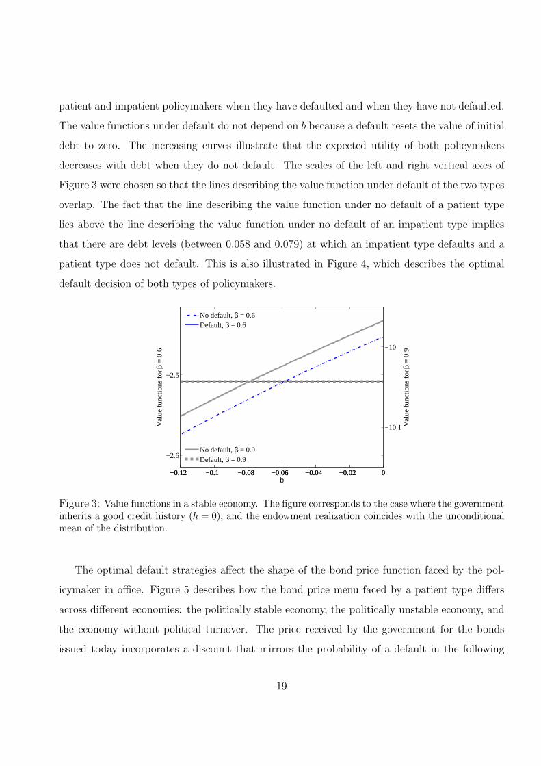
policymaker. Figure 9 helps one understand why impatient policymakers choose lower issuance

volumes. It illustrates how bond price schedules faced by impatient policymakers display three

steps as do the schedules faced by patient policymakers. If the current policymaker is impatient, it

is highly likely that the next-period policymaker will also be impatient. Given that the impatient

type defaults on “intermediate” debt levels, lenders demand a high discount for “intermediate”

borrowing levels, which explains why the intermediate step in Figure 9 is close to zero. The fact

that the bond price for intermediate issuance levels is significantly lower than the bond price for

“low” issuance levels leads impatient governments to choose “low” issuance levels. As explained

before, in politically stable economies, patient governments often choose intermediate issuance

levels. That is, our theory predicts that even though impatient governments assign more weight

to current utility flows, they may decide to borrow less than patient governments.

The second distinctive feature of political defaults is that post-default equilibrium spreads are

lower than pre-default spreads. Before a political default, patient governments choose “interme-

25

−0.08 −0.075 −0.07 −0.065 −0.06 −0.055 −0.05 −0.045 −0.040

0.2

0.4

0.6

0.8

1

b’

Bon

d pr

ice

−0.08 −0.075 −0.07 −0.065 −0.06 −0.055 −0.05 −0.045 −0.04

π = 1.5%

π = 2.5%

Figure 9: Bond price faced by an impatient policymaker in economies with high and low political stabil-ity. The graph considers the case in which the endowment realization coincides with the unconditionalmean of the distribution and in which the government has defaulted today.

diate” issuance levels and, therefore, they pay “intermediate” spreads. After a political default,

impatient governments choose “low” issuance levels and, therefore, they pay “low” spreads. That

is, our theory predicts that more investor-friendly governments pay higher spreads in equilibrium

than less investor-friendly governments. On the contrary, if a default is non-political, post-default

spreads are similar to pre-default spreads. In our model, if there is no political turnover, lenders

have no reason to offer a different treatment to a country that has defaulted in the past and,

in general, there is no reason for the equilibrium government’s behavior after the default to be

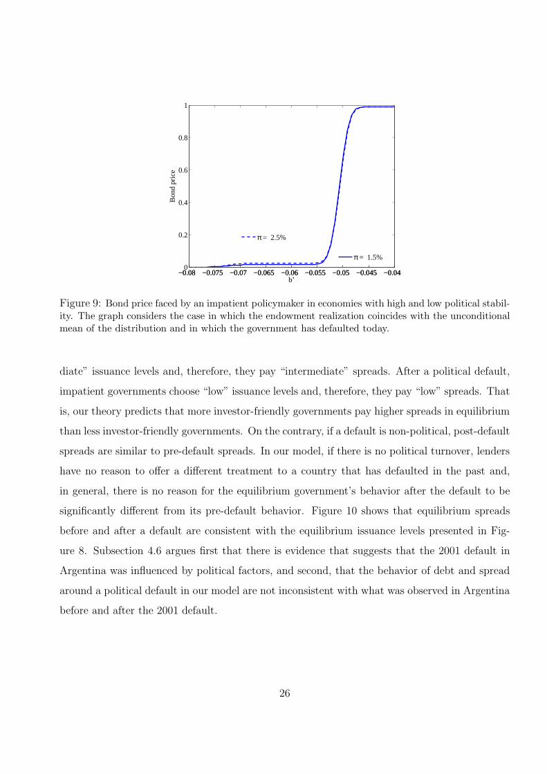
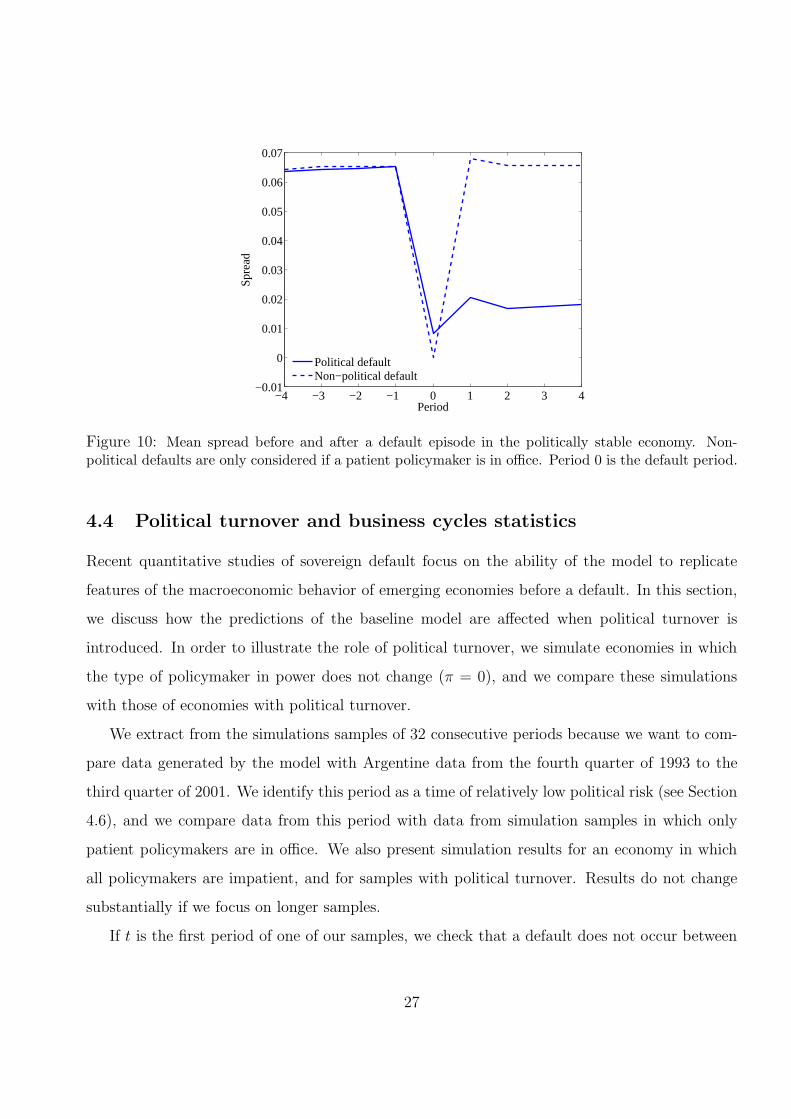
significantly different from its pre-default behavior. Figure 10 shows that equilibrium spreads

before and after a default are consistent with the equilibrium issuance levels presented in Fig-

ure 8. Subsection 4.6 argues first that there is evidence that suggests that the 2001 default in

Argentina was influenced by political factors, and second, that the behavior of debt and spread

around a political default in our model are not inconsistent with what was observed in Argentina

before and after the 2001 default.

26

−4 −3 −2 −1 0 1 2 3 4−0.01

0

0.01

0.02

0.03

0.04

0.05

0.06

0.07

Spr

ead

Period

Political defaultNon−political default

Figure 10: Mean spread before and after a default episode in the politically stable economy. Non-political defaults are only considered if a patient policymaker is in office. Period 0 is the default period.

4.4 Political turnover and business cycles statistics

Recent quantitative studies of sovereign default focus on the ability of the model to replicate

features of the macroeconomic behavior of emerging economies before a default. In this section,

we discuss how the predictions of the baseline model are affected when political turnover is

introduced. In order to illustrate the role of political turnover, we simulate economies in which

the type of policymaker in power does not change (π = 0), and we compare these simulations

with those of economies with political turnover.

We extract from the simulations samples of 32 consecutive periods because we want to com-

pare data generated by the model with Argentine data from the fourth quarter of 1993 to the

third quarter of 2001. We identify this period as a time of relatively low political risk (see Section

4.6), and we compare data from this period with data from simulation samples in which only

patient policymakers are in office. We also present simulation results for an economy in which

all policymakers are impatient, and for samples with political turnover. Results do not change

substantially if we focus on longer samples.

If t is the first period of one of our samples, we check that a default does not occur between

27

periods t − 2 and t + 31. This makes our samples free from the effects of within-sample de-

fault episodes and, therefore, comparable with the Argentine sample (the Argentine government

honored its debt between the fourth quarter of 1993 and the third quarter of 2001).

From the simulations of economies without political turnover, we extract the first 500 samples

before a default. From the simulations of economies with political turnover, we present two sets of

results. First, we extract the first 500 samples that satisfy the following criteria: (i) the beginning

of the sample is determined by a change of the policymaker in power, from an impatient type

to a patient type, (ii) the patient type remains in office for 32 consecutive periods, and (iii) in

the first period after the end of the sample, an impatient policymaker gains power and declares

a default. We also present unconditional results using the first 500 samples before any type of

default episode and without imposing any restriction on the type of policymaker in power.

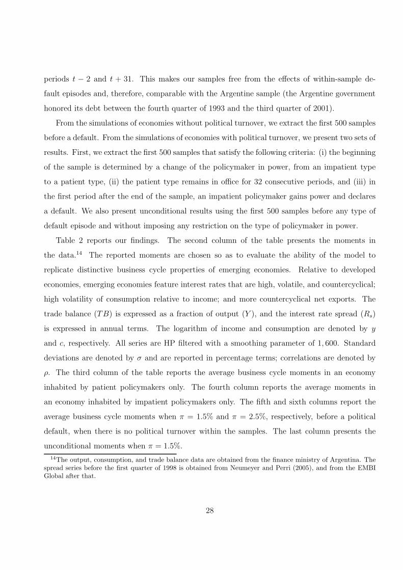
Table 2 reports our findings. The second column of the table presents the moments in

the data.14 The reported moments are chosen so as to evaluate the ability of the model to

replicate distinctive business cycle properties of emerging economies. Relative to developed

economies, emerging economies feature interest rates that are high, volatile, and countercyclical;

high volatility of consumption relative to income; and more countercyclical net exports. The

trade balance (TB) is expressed as a fraction of output (Y ), and the interest rate spread (Rs)

is expressed in annual terms. The logarithm of income and consumption are denoted by y

and c, respectively. All series are HP filtered with a smoothing parameter of 1, 600. Standard

deviations are denoted by σ and are reported in percentage terms; correlations are denoted by

ρ. The third column of the table reports the average business cycle moments in an economy

inhabited by patient policymakers only. The fourth column reports the average moments in

an economy inhabited by impatient policymakers only. The fifth and sixth columns report the

average business cycle moments when π = 1.5% and π = 2.5%, respectively, before a political

default, when there is no political turnover within the samples. The last column presents the

unconditional moments when π = 1.5%.

14The output, consumption, and trade balance data are obtained from the finance ministry of Argentina. Thespread series before the first quarter of 1998 is obtained from Neumeyer and Perri (2005), and from the EMBIGlobal after that.

28

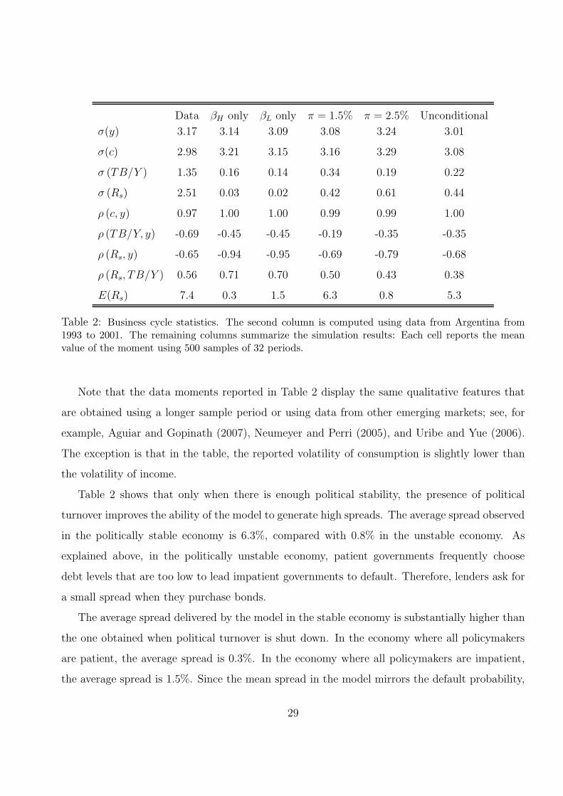
Data βH only βL only π = 1.5% π = 2.5% Unconditional

σ(y) 3.17 3.14 3.09 3.08 3.24 3.01

σ(c) 2.98 3.21 3.15 3.16 3.29 3.08

σ (TB/Y ) 1.35 0.16 0.14 0.34 0.19 0.22

σ (Rs) 2.51 0.03 0.02 0.42 0.61 0.44

ρ (c, y) 0.97 1.00 1.00 0.99 0.99 1.00

ρ (TB/Y, y) -0.69 -0.45 -0.45 -0.19 -0.35 -0.35

ρ (Rs, y) -0.65 -0.94 -0.95 -0.69 -0.79 -0.68

ρ (Rs, TB/Y ) 0.56 0.71 0.70 0.50 0.43 0.38

E(Rs) 7.4 0.3 1.5 6.3 0.8 5.3

Table 2: Business cycle statistics. The second column is computed using data from Argentina from1993 to 2001. The remaining columns summarize the simulation results: Each cell reports the meanvalue of the moment using 500 samples of 32 periods.

Note that the data moments reported in Table 2 display the same qualitative features that

are obtained using a longer sample period or using data from other emerging markets; see, for

example, Aguiar and Gopinath (2007), Neumeyer and Perri (2005), and Uribe and Yue (2006).

The exception is that in the table, the reported volatility of consumption is slightly lower than

the volatility of income.

Table 2 shows that only when there is enough political stability, the presence of political

turnover improves the ability of the model to generate high spreads. The average spread observed

in the politically stable economy is 6.3%, compared with 0.8% in the unstable economy. As

explained above, in the politically unstable economy, patient governments frequently choose

debt levels that are too low to lead impatient governments to default. Therefore, lenders ask for

a small spread when they purchase bonds.

The average spread delivered by the model in the stable economy is substantially higher than

the one obtained when political turnover is shut down. In the economy where all policymakers

are patient, the average spread is 0.3%. In the economy where all policymakers are impatient,

the average spread is 1.5%. Since the mean spread in the model mirrors the default probability,

29

an economy in which investor-friendly governments alternate in power with less investor-friendly

governments has a higher default probability than one where governments are never friendly

to investors. It is the presence of political turnover—and not the low discount factor of the

impatient type—that is crucial for generating a higher default probability.

Mechanically, political turnover enables the model to generate a higher average spread because

it smoothes out the bond price function, i.e., political turnover makes the bond price less sensitive

to the issuance volume. With a smoother price function, a given decrease in the bond price

allows for a larger increase in the issuance level. This makes the choice of lower bond prices more

attractive and induces the government to pay a higher spread.15

Table 2 illustrates the non-monotonic relationship between the mean spread and the degree

of political stability. The third column can be interpreted as an extreme case where π = 0 and

the patient policymaker is in power in the first period. Starting from this case, a decrease in the

level of political stability to π = 1.5% increases the mean spread from 0.3% to 6.3%. A further

decrease in the level of political stability to π = 2.5% decreases the mean spread from 6.3% to

0.8%.

There are two forces through which changes in π affect the mean spread. First, an increase

in π increases the spread paid at intermediate borrowing levels. Second, an increase in π makes

intermediate borrowing levels less attractive and, therefore, less frequent in equilibrium. The

first effect is dominant when π is sufficiently low, i.e., when the discount in the bond price at

intermediate borrowing levels is sufficiently low. For a low π, the government chooses interme-

diate borrowing levels often, and small changes in π have a direct effect on the spread paid at

these borrowing levels. The second effect is dominant when π is sufficiently high and, therefore,

intermediate borrowing levels are chosen less frequently.

The previous discussion illustrates that in our model, the degree of political stability affects

spreads mainly by changing the shape of the bond price. This is not the case in the environments

studied by Amador (2003) and Cuadra and Sapriza (2008). In their models, political stability

affects spreads by changing the value of future utility flows.

15In the economy with low political stability, a smoother price function does not increase the mean spreadbecause intermediate debt levels are rarely observed in equilibrium.

30

In addition, Table 2 shows that the presence of political turnover enables the model to generate

higher spread volatility. In the economy with high political stability, the standard deviation

of the spread is 0.42%. In contrast, we find a standard deviation of 0.03% in the economies

without political turnover. The higher spread volatility is also a consequence of a smoother bond

price function. It should be stressed that this higher volatility is not driven by the presence of

policymakers of different types (who are willing to pay different spread levels) in the simulation

samples. Recall that this higher standard deviation is computed using samples in which only

patient policymakers are in power.

The last column of Table 2 shows that, in the politically stable economy, the unconditional

business cycle moments are similar to the ones obtained when only pre-political-default samples

without within-sample political turnover are considered (fifth column). This is the case because

most defaults in the stable economy are political defaults. In addition, the table shows that the

introduction of political turnover does not significantly affect other business cycle moments.16

4.5 Equilibrium with a completely myopic type

In this section, we study the stable (π = 1.5%) and unstable (π = 2.5%) economies assuming

the impatient type is completely myopic (βL = 0). This corresponds to the case studied in Cole

et al. (1995), and Alfaro and Kanczuk (2005). Chatterjee et al. (2007b) consider cases where the

impatient type is fully myopic and nearly myopic (βL = 0.05).

We find that when the impatient type is fully myopic, our model generates predictions that are

strongly counterfactual. Spreads paid by impatient governments are too high. For instance, the

maximum annualized spread paid by an impatient government in the politically stable (unstable)

economy is 2, 062, 878, 145% (267, 244, 563%). Even though completely myopic types always

16As in the benchmark case without heterogeneity, one may think that the debt levels generated by the modelare low (between 5% and 7% of quarterly output). In part, this is because we do not assume that a defaultingeconomy is excluded from capital markets; see Hatchondo et al. (2007b). Furthermore, simplifying assumptionslimit the ability of the model to generate higher debt levels. For instance, it is assumed that governments cannotsave and borrow at the same time, that defaults imply a total repudiation of debt, and that all the debt is heldby foreigners. Moreover, there are costs of defaulting that are not present in the model; see Hatchondo et al.(2007a) for a discussion of defaulting cost. Since our model builds on the baseline framework that has been usedin recent quantitative studies and also shares the same parameterization, it generates debt levels comparable tothe ones in those studies.

31

default, a completely myopic government may be offered a positive bond price, because with

positive probability, the next-period default decision is going to be made by a patient type—who

would choose to honor its debt. Since the impatient type only cares about current consumption,

it is optimal for it to issue bonds even when these bonds are sold at a large discount.

We also find that when βL = 0, patient governments often prefer “intermediate” issuance

levels over “low” issuance levels even in the politically unstable economy. This is the case

because the extra borrowing that can be obtained by paying the intermediate spread level is

large—i.e., the length of the intermediate step in the bond price function faced by patient types

is large. Thus, it pays off to choose intermediate spread levels as this enables patient governments

to increase the borrowing level by a relatively large amount. This illustrates how, in general,

the larger the difference between βH and βL (the more politically polarized is the economy), the

more likely patient governments choose debt levels that would lead impatient governments to

default. When βL = 0, for any borrowing level, a patient government would have to pay at least

the intermediate spread level.

4.6 The 2001 default in Argentina

In this subsection, we present a brief case study of the 2001 default episode in Argentina. We

first argue that political circumstances around this default episode are similar to the ones in the

political defaults of our model. Then, we show that the behavior of the spread and the debt level

in Argentina around the default episode are not inconsistent with the predictions of our theory.

Let us discuss first why the default episode in Argentina can be interpreted as a political

default. Recall that we defined political defaults as episodes triggered by political turnover.

Political turnover preceded the default in Argentina. After president De La Rua resigned on

December 20, 2001, Congress appointed Rodriguez Saa as the interim president on December

23, 2001. As discussed by Sturzenegger and Zettelmeyer (2006), the next day, Rodriguez Saa

announced the suspension of all payments on debt instruments.

In addition, in our model, a political default occurs when an investor-friendly government is

replaced by a government that is less friendly to investors. Everything else being equal, political

32

risk for investors (default risk) is higher (lower) when impatient (patient) policymakers are in

power. Thus, our model predicts that—everything else being equal—pre-political-default levels

of political risk for investors are lower than post-political-default levels. In order to gauge whether

such a change in political risk for investors occurred in Argentina, we look at the composite index

of political risk for investors constructed by the International Country Risk Guide (ICRG). This

index of political risk is one of the three components of the overall risk index constructed by the

ICRG (the other two indexes are the financial risk index and the economic risk index). The index

of political risk is supposed to reflect political risk only, independently from economic risk and

financial risk (which are captured by the other two indexes).17 Thus, the index of political risk

does not necessarily mirror default risk. In fact, we will explain that default risk in Argentina

was presumably higher (the spread was higher) when political risk was lower.

We compare the mean value of the index of political risk in the eight years prior to the default

date with the mean value between the default date and June 2006. The index of political risk

for investors is such that a higher value indicates less political risk. The pre-default mean value

of the index is 74.4, and the post-default value is 64.3.18 If we identify the higher (lower) values

of the index with an “investor-friendly” (less friendly) type being in power, the variations of the

index of political risk in Argentina suggest that the default episode in Argentina is characterized

by the type of regime change our model indicates is necessary for political defaults to occur.

That is, in Argentina, post-default governments were considered more risky for investors than

pre-default governments.19

17The ICRG indexes are widely used in empirical studies. See, for example, Erb et al. (1996), Erb et al. (2003),Bilson et al. (2002), Bekaert and Harvey (1996), Bekaert et al. (2007a), and Bekaert et al. (2007b). These studiesprovide a more thorough discussion of the indexes.

18The higher political risk after the default does not seem to be a mere consequence of the default itself. Othercountries do not exhibit such large increase in political risk after defaulting. For instance, when we repeat thesame exercise conducted for Argentina for the recent defaults in Ecuador (1999), Pakistan (1999), Russia (1998),and Uruguay (2003), we find that (i) in Ecuador, the pre-default mean value of the index of political risk forinvestors is 60.7, and the post-default value is 57.0; (ii) in Pakistan, the pre-default value is 51.4, and the post-default value is 47.3; (iii) in Russia, the pre-default value is 56.7 (considering data since April 1992), and thepost-default value is 60.7; and (iv) in Uruguay, the pre-default value is 72.1, and the post-default value is 72.4.

19Of course, higher values of the index of political risk cannot be mapped exactly with more patient governmentsin our model. The index is a noisy measure of the government type. For instance, while our stylized model assumesthat the government stability parameter (π) is constant, the index may be affected by changes in governmentstability. However, the decrease in the average value of the index after the default is indicative of a regime change.

33

Furthermore, Argentina exhibits a relatively high degree of political stability, a feature that

this paper identifies as necessary for the occurrence of political defaults. In the ten years prior

to the default episode, the index of political risk is higher than the average post-default index.

This indicates that it is plausible that investor-friendly governments in Argentina may have been

perceived as stable during the 1990s.

As explained in Section 4.3, our theory predicts that a distinctive feature of political defaults

is that post-default debt levels are lower than pre-default levels. This is consistent with what

we observed in Argentina. The per capita public external debt in Argentina expressed in 2006

U.S. dollars ranged from $2084 to $2801 between March 1994 and December 2001. It was $2659

in December 2001. After the default, it was $1311 in March 2006 (without considering $121 of

arrears).

Our theory predicts that another distinctive feature of political defaults is that post-default

spreads are lower than pre-default spreads. This seems consistent with what we observed in

Argentina. As reported in Table 2, the average annualized spread for Argentina between the

fourth quarter of 1993 and the third quoter of 2001 is 7.4%. The average spread for Argentina

between the third quarter of 2005 and the second quarter of 2007 is 3.4%.20 Thus, as our theory

predicts, governments that were considered to be “less friendly” to investors paid lower spreads

in Argentina.

5 Conclusions and extensions

This paper introduces a stylized political process into the framework used in recent quantita-

tive studies of sovereign default. We show that a default episode is likely to be triggered by

political turnover only if there is enough political stability in the economy and investor-friendly

governments encounter sufficiently poor economic conditions during their tenure. The presence

of political turnover enables the model to generate (i) a moderate correlation between economic

conditions and default decisions, (ii) lower borrowing levels after a default episode, and (iii) a

20We do not consider the spread between the default episode in 2001 and the debt exchange in 2005, becauseduring that period, the spread is computed using the price of defaulted bonds and, therefore, does not reflect theinterest rate at which Argentina borrowed over that period.

34

higher and more volatile spread.

Our stylized political process simplifies the analysis and enables us to provide a transparent

description of the mechanism behind our results. Allowing for a richer political process could

improve the performance of the model. For example, if the probability of political turnover

reacts to changes in output or consumption, the model may be able to generate a higher spread

volatility.

35

References

Aguiar, M. and G. Gopinath, “Defaultable debt, interest rates and the current account,” Journal

of International Economics 69 (2006), 64–83.

Aguiar, M. and G. Gopinath, “Emerging markets business cycles: the cycle is the trend,” Journal

of Political Economy 115 (2007), 69–102.

Alfaro, L. and F. Kanczuk, “Sovereign debt as a contingent claim: a quantitative approach,”

Journal of International Economics 65 (2005), 297–314.

Amador, M., “A Political Economy Model of Sovereign Debt Repayment,” mimeo, Stanford

University, 2003.

Arellano, C., “Default Risk and Income Fluctuations in Emerging Economies,” American Eco-

nomic Review 98 (2008), 690–712.

Arellano, C. and A. Ramanarayanan, “Default and the term structure in sovereign bonds,”

mimeo, University of Minnesota, 2006.

Arteta, C. and G. Hale, “Sovereign Debt Crises and Credit to the Private Sector,” Journal of

International Economics 74 (2008), 53–69.

Athreya, K., “Welfare Implications of the Bankruptcy Reform Act of 1999,” Journal of Monetary

Economics 49 (2002), 1567–1595.

Athreya, K. B. and H. P. Janicki, “Credit exclusion in quantitative models of bankruptcy: does

it matter?,” Economic Quarterly 92 (2006), 17–50.

Bai, Y. and J. Zhang, “Financial integration and international risk sharing,” mimeo, Michigan

University, 2006.

Balkan, E., “Political Instability, Country Risk and Probability of Default,” Applied Economics

24 (1992), 999–1008.

36

Bekaert, G. and C. R. Harvey, “Emerging Markets Finance,” Journal of Empirical Finance 10

(1996), 46–58.

Bekaert, G., C. R. Harvey and C. Lundblad, “Political Risk, Financial Risk and Economic Risk,”

Review of Financial Studies 20 (2007a), 1783–1831.

Bekaert, G., C. R. Harvey, C. Lundblad and S. Siegel, “Global Growth Opportunities and Market

Integration,” The Journal of Finance 62 (2007b), 1081–1137.

Bi, R., “Debt Dilution and the Maturity Structure of Sovereign Bonds,” mimeo, University of

Maryland, 2006.

Bilson, C., T. Brailsford and V. Hooper, “The Explanatory Power of Political Risk in Emerging

Markets,” International Review of Financial Analysis 11 (2002), 1–27.

Chatterjee, S., D. Corbae, M. Nakajima and J.-V. Rıos-Rull, “A Quantitative Theory of Unse-

cured Consumer Credit with Risk of Default,” Econometrica 75 (2007a), 1525–1589.

Chatterjee, S., D. Corbae and J.-V. Rıos-Rull, “Credit Scoring and Competitive Pricing of De-

fault Risk,” mimeo, University of Texas at Austin, 2007b.

Citron, J. and G. Nickelsburg, “Country Risk and Political Instability,” Journal of Development

Economics 25 (1997), 385–392.

Cole, H., J. Dow and W. English, “Default, settlement, and signaling: lending resumption in a

reputational model of sovereign debt,” International Economic Review 36 (1995), 365–385.

Cuadra, G. and H. Sapriza, “Sovereign default, terms of trade, and interest rates in emerging

markets,” working paper 2006-01, Banco de Mexico, 2006.

Cuadra, G. and H. Sapriza, “Sovereign default, interest rates and political uncertainty in emerg-

ing markets,” Journal of International Economics (2008), forthcoming.

Eaton, J. and M. Gersovitz, “Debt with potential repudiation: theoretical and empirical analy-

sis,” Review of Economic Studies 48 (1981), 289–309.

37

Eichengreen, B. and R. Portes, “Debt Restructuring With and Without the IMF,” mimeo, UC

Berkeley, 2000.

Erb, C., C. R. Harvey and T. Viskanta, “Political Risk, Financial Risk and Economic Risk,”

Financial Analysts Journal 52 (1996), 28–46.

Erb, C., C. R. Harvey and T. Viskanta, “Expected Returns and Volatility in 135 Countries,”

Journal of Portfolio Management 10 (2003), 3–56.

Eyigungor, B., “Sovereign Debt Spreads in a Markov Switching Regime,” mimeo, UCLA, 2006.

Gelos, G., R. Sahay and G. Sandleris, “Sovereign Borrowing by Developing Countries: What

Determines Market Access?,” working paper 04/221, IMF, 2004.

Goretti, M., “The Brazilian currency turmoil of 2002: a nonlinear analysis,” International Jour-

nal of Finance and Economics 10 (2005), 289–306.

Hatchondo, J. C. and L. Martinez, “Long-duration Bonds and Sovereign Defaults,” working

paper 08-2, Federal Reserve Bank of Richmond, 2008.

Hatchondo, J. C., L. Martinez and H. Sapriza, “On the cyclicality of the interest rate in emerging

economies: solution methods matter,” mimeo, Federal Reserve Bank of Richmond, 2006.

Hatchondo, J. C., L. Martinez and H. Sapriza, “The economics of sovereign default,” Economic

Quarterly 93 (2007a), 163–197.

Hatchondo, J. C., L. Martinez and H. Sapriza, “Quantitative Models of Sovereign Default and

the Threat of Financial Exclusion,” Economic Quarterly 93 (2007b), 251–286.

IMF, “Sovereign Debt Restructurings and the Domestic Economy Experience in Four Resent

Cases,” Policy development and review department, 2002.

Kaminsky, G. and C. M. Reinhart, “The Twin Crises: The Causes of Banking and Balance of

Payments Crises,” American Economic Review 89 (1999), 473–500.

38

Kobayashi, K., “Payment uncertainty, the division of labor, and productivity declines in great

depressions,” Review of Economic Dynamics 9 (2006), 715–741.

Kohlscheen, E., “Constitutions Rule,” mimeo, IIES, 2003.

Krusell, P. and A. Smith, “Consumption-savings decisions with quasi-geometric discounting,”

Econometrica 71 (2003), 365–375.

Kumhof, M., “Fiscal crisis resolution: taxation versus inflation,” mimeo, Stanford University,

2004.

Kumhof, M. and E. Tanner, “Government Debt: A Key Role in Financial Intermediation,”

working paper 05/57, IMF, 2005.

Li, W. and P.-D. Sarte, “U.S. consumer bankruptcy choice: The importance of general equilib-

rium effects,” Journal of Monetary Economics 53 (2006), 613–631.

Livshits, I., J. MacGee and M. Tertilt, “Consumer Bankruptcy: A Fresh Start,,” American

Economic Review 97 (2007), 402–418.

Lizarazo, S., “Sovereign risk and risk averse international investors,” mimeo, ITAM, 2005.

Lizarazo, S., “Contagion of financial crises in sovereign debt markets,” mimeo, ITAM, 2006.

Mendoza, E. and V. Yue, “A Solution to the Default Risk-Business Cycle Disconnect,” mimeo,

New York University, 2007.

Meyersson, E., “Debt intolerance and institutions, an empirical investigation into the institutional

effect of sovereign debt,” mimeo, Stockholm University, 2006.

Moser, C., “The Impact of Political Risk on Sovereign Bond Spreads. Evidence from Latin

America,” mimeo, University of Mainz, 2006.

Neumeyer, P. and F. Perri, “Business cycles in emerging economies: the role of interest rates,”

Journal of Monetary Economics 52 (2005), 345–380.

39

Pimentel, L. and H. Murphy, “Ecuador’s Bonds Fall on Correa’s Restructure Pledge, Oil Prices,”

Bloomberg (2006), november 17.

Reinhart, C., K. S. Rogoff and M. A. Savastano, “Debt Intolerance,” Brookings Papers on Eco-

nomic Activity 34 (2003), 1–74.

Sandleris, G., “Sovereign Defaults: Information, Investment and Credit,” mimeo, Johns Hopkins

University, 2006.

Santiso, J., The Political Economy of Emerging Markets: Actors, Institutions and Crisis in Latin

America (New York / London, Palgrave, 2003).

Schmitt-Grohe, S. and M. Uribe, “Closing small open economy models,” Journal of International

Economics 61 (2003), 163–185.

Sturzenegger, F. and J. Zettelmeyer, “Defaults in the 90s,” mimeo, Universidad Torcuato Di

Tella, 2006.

Tomz, M. and M. L. J. Wright, “Do Countries Default in “Bad Times”?,” Journal of the European

Economic Association 5 (2007), 352–360.

Uribe, M. and V. Yue, “Country spreads and emerging countries: Who drives whom?,” Journal

of International Economics 69 (2006), 6–36.

Van Rijckeghem, C. and B. Weder, “The Politics of Debt Crises,” mimeo, University of Mainz,

2004.

Wright, M. L. J., “Reputations and Sovereign Debt,” mimeo, Stanford University, 2002.

Wright, M. L. J., “Coordinating Creditors,” American Economic Review Papers and Proceedings

95 (2005), 388–392.

Yue, V., “Sovereign default and debt renegotiation,” mimeo, NYU, 2005.

40