HAL Id: halshs-00692038https://halshs.archives-ouvertes.fr/halshs-00692038

Preprint submitted on 27 Apr 2012

HAL is a multi-disciplinary open accessarchive for the deposit and dissemination of sci-entific research documents, whether they are pub-lished or not. The documents may come fromteaching and research institutions in France orabroad, or from public or private research centers.

L’archive ouverte pluridisciplinaire HAL, estdestinée au dépôt et à la diffusion de documentsscientifiques de niveau recherche, publiés ou non,émanant des établissements d’enseignement et derecherche français ou étrangers, des laboratoirespublics ou privés.

The sovereign default puzzle: Modelling issues andlessons for Europe

Daniel Cohen, Sébastien Villemot

To cite this version:Daniel Cohen, Sébastien Villemot. The sovereign default puzzle: Modelling issues and lessons forEurope. 2012. �halshs-00692038�

WORKING PAPER N° 2012 – 21

The sovereign default puzzle: Modelling issues and lessons for Europe

Daniel Cohen Sébastien Villemot

JEL Codes: F34

Keywords: Sovereign debt ; Lévy stochastic processes

PARIS-JOURDAN SCIENCES ECONOMIQUES 48, BD JOURDAN – E.N.S. – 75014 PARIS

TÉL. : 33(0) 1 43 13 63 00 – FAX : 33 (0) 1 43 13 63 10

www.pse.ens.fr

CENTRE NATIONAL DE LA RECHERCHE SCIENTIFIQUE – ECOLE DES HAUTES ETUDES EN SCIENCES SOCIALES

ÉCOLE DES PONTS PARISTECH – ECOLE NORMALE SUPÉRIEURE – INSTITUT NATIONAL DE LA RECHERCHE AGRONOMIQUE

The sovereign default puzzle:

Modelling issues and lessons for Europe∗

Daniel Cohen† Sebastien Villemot‡

April 26, 2012

Abstract

Why do countries default? This seemingly simple question has yet to be adequately

answered in the literature. Indeed, prevailing modelling strategies compel the to choose

between two unappealing model features: depending on the cost of default selected by the

modeler, either the debt ratios are too high and the probability of default is too low or

the opposite is true. In view of the historical evidence that countries always default after a

crisis, we propose a novel approach to the theory of debt default and develop a model that

matches the key stylized facts regarding sovereign risk.

Keywords: Sovereign debt, Levy stochastic processes

JEL Classification: F34

1 Introduction

Europe has recently been hit by a sovereign debt crisis which has caused three of its members

to be ousted from financial markets. Those three countries, Greece, Ireland and Portugal, had

to ask for the support of the other eurozone countries to refinance their debt. Additionally,

in the case of Greece the eventual implementation of a nominal haircut of more than 50%

was decided. In response to this unexpected crisis, Europe decided to impose a much stricter

budgetary discipline, aiming for a near zero deficit rule. How did the eurozone suddenly become

so vulnerable to sovereign risk? Is Europe overreacting by imposing budget constraints that are

too restrictive?

Sovereign debt crisis specialists have been asked for answers. Trying to understand why

some countries default is the theme of a large body of literature. Reinhart et al. (2003) have

investigated the nature of what they called the “debt intolerance” of many countries over the

centuries. Greece is certainly one of these, having already defaulted many times over the past

two centuries. The key paradox of the academic literature however, is that it is actually very

hard to satisfactorily fit the data on default probabilities and debt levels. Work by Aguiar and

∗Many thanks to Houtan Bastani for proofreading this text.†Paris School of Economics and CEPR. E-mail: daniel.cohen@ens.fr‡Paris School of Economics and CEPREMAP. E-mail: sebastien.villemot@ens.fr

1

Gopinath (2006) or Arellano (2008) for instance struggled with the fact that a debt-to-GDP

ratio in excess of only 5% could trigger a default within reasonably calibrated models. These

papers have, on the surface, trivialized the problem, as almost any level of debt seems to create

a risk of default.

These difficulties led Rogoff (2011) to argue that the narrative approach to debt default,

as exemplified in Reinhart and Rogoff (2009), does a better job at understanding default than

simulated models. This is clearly a provocative statement. Barring a calibrated model, how

can one think about what the proper debt levels should be? Further, how can one rationalize

the eurozone policymakers’ attempts to set safe debt levels in order to avoid another crisis?

In previous models of sovereign risk, default is a costly decision that the country weighs

against the alternative of repaying its debt. From a modeler’s perspective, the following trade

off arises. Either the cost of default is high, in which case high debt-to-GDP ratios can be

sustained at the expense of a low frequency of default, as countries don’t default when the costs

are high. Or the cost of default is set at low levels, in which case the frequency of default can

fit the data, but the sustainable debt levels become abnormally low; this is the outcome of most

calibrated models today.

In this paper, we revisit existing sovereign debt models and amend them in order to get

predictions which better fit real world debt levels. The key motivation of our analysis comes

from the following observation of which the Greek crisis is one illustration: countries usually do

not want to default unilaterally. In fact, as well documented by the Inter-American Development

Bank (2007) and Levy-Yeyati and Panizza (2011), in all cases of sovereign debt crises but one,

the “decision” to default was never really a decision of the country: it came after the crisis

already took place. The only case of a “strategic default” is Ecuador in 2009. This leads us

to the following new modelling assumption. In our model, the sequencing of events is inverted:

the crisis begins before the decision to default has been taken. Think of a bank panic or a

temporary collapse of a key industrial sector. In these “trembling times,” the cost of default

becomes lower as the financial panic or the economic meltdown already happened. Default does

add extra costs, but lower than those which would have be borne in “normal times.” With this

distinction, we show that we can simultaneously model high levels of debt with a high frequency

of default.

The paper is organized as follows. In section 2, we provide a brief overview of recent debt

models, then convey an intuitive outline of our contribution. In section 3, relying on the key

insights of the theory of Levy processes which allows one to split output into a Brownian and

a Poisson process, we develop a simplified model. We interpret “trembling times” as shocks

generated by Poisson jumps; in our model, they are those which have the potential to generate

default. We demonstrate that Brownian shocks instead do not have the property of triggering

default events. In a continuous time setting, we show that an optimizing social planner should

always absorb Brownian shocks so as to avoid default. This allows us to discriminate among

two key causes of debt crises. One is the failure to adjust in real time to a smooth shock, the

solution to which being to have a more efficient monitoring of intra-annual deficit. The second is

2

the challenge of a discontinuous shock, which is where the core problem comes from. We argue

that previous models’ difficulties in replicating default owe much to the lack of understanding

of this distinction. In section 4, we then simulate the full-fledged version of the model using the

standard assumptions of emerging economies. In section 5, we recast the model in the European

setting and draw some policy conclusions for the eurozone. Section 6 concludes.

2 Calibrating sovereign debt models

Calibrated models of sovereign debt owe much to the papers by Aguiar and Gopinath (2006),

Arellano (2008) and Mendoza and Yue (2011), which followed in the (earlier) tradition of Eaton

and Gersovitz (1981), Cohen and Sachs (1986) and Bulow and Rogoff (1989).

Their framework is as follows. An indebted country can decide to default, paying as a

consequence a (lump-sum) cost. This cost sets the upper limit of debt, as lenders attempt to

monitor the risks. These models have successfully reproduced key business cycle correlations

regarding aggregate spending and balance of payments in particular. The problem encountered

by these models however, is that they meet great difficulties in calibrating reasonable debt

thresholds and probabilities of default at the same time. Table 1 summarizes the key results

obtained by several recent papers along these dimensions.

Table 1: Overview of mean debt-to-GDP ratios and default probabilities in the literature

Debt-to-GDP DefaultPaper Main feature mean ratio probability

(%, annual) (%, annual)Arellano (2008) Non-linear default cost 1 3.0Aguiar and Gopinath (2006) Shocks to GDP trend 5 0.9Cuadra and Sapriza (2008) Political uncertainty 2 4.8Fink and Scholl (2011) Bailouts and conditionality 1 5.0Yue (2010) Endogenous recovery 3 2.7Mendoza and Yue (2011) Endogenous default cost 6 2.8Hatchondo and Martinez (2009) Long-duration bonds 5 2.9Benjamin and Wright (2009) Endogenous recovery 16 4.4Chatterjee and Eyigungor (2011) Long-duration bonds 18 6.6

Most papers report the debt-to-GDP ratio using GDP measured at a quarterly frequency; we chooseto use GDP measured at an annual frequency, since this is the convention used by policymakers and inthe policy debate. For Aguiar and Gopinath (2006), we report results for their model II (with shocksto GDP trend). For Arellano (2008) and Aguiar and Gopinath (2006), the reported values come fromHatchondo et al. (2010) who resimulate these models using more precise numerical techniques. ForHatchondo and Martinez (2009), the reported values are those obtained for their λ parameter equalto 20%.

Before discussing the results of these papers, one should note the improbably high discount

factor that some models have to rely on to sustain their equilibrium. For example, Yue (2010)

and Aguiar and Gopinath (2006) set respective values of 0.72 and 0.8 for the (quarterly!)

discount factor. This high impatience helps to generate frequent defaults and a desire to hold

debt, but it is unrealistically high, even when accounting for political instability. Others, like

3

Arellano (2008), Benjamin and Wright (2009) or Chatterjee and Eyigungor (2011) use values

close to 0.95, which is more realistic. We will use this last value in our simulations (see section

4.4).

In order to fit the conventional wisdom of markets and international financial institutions,

one would want a model that could predict:

• Threshold debt levels in the vicinity of 40% of yearly GDP. The mean debt-to-GDP ratio in

2009 was 42% across countries, according to our computations using World Bank (2010).

Note that World Bank (2004) classifies as “severely indebted” countries with a debt-to-

GNI ratio above 80%, and as “moderately indebted” countries with a ratio above 48%:

our target of 40% is therefore in the lower end of the range of interest; in section 5.3 we

show how to reach higher levels of debts.

• Annual default probabilities in the range of 3%. Yue (2010) reports that the average default

rate of Argentina since 1824 is 2.7%. Benjamin and Wright (2009) estimate an average

default rate across countries of 4.4% for the period 1989–2006. In the data collected by

Cohen and Valadier (2011) over the period 1970–2007, which includes “soft defaults” such

as IMF loans, an even higher probability of default of about 7% is documented. We stick

to the 3% target preferred by most papers, to make the comparison easier.

Even though many papers listed in Table 1 reach the target in terms of default probabilities,

they all fail with respect to the sustainable debt ratios; the two best results along this dimension

are Benjamin and Wright (2009) and Chatterjee and Eyigungor (2011) who respectively reach

debt levels of 16% and 18% of yearly GDP.1

We now turn to the task of proposing a quantitative sovereign debt model that matches

the two stylized facts regarding debt levels and default probabilities, with a minimal departure

from the canonical model. Our modifications hinge on the following arguments:

1. The cost of default in the models found in the literature is too low to be true. Based

on historical averages they typically assume that it usually takes two and a half years of

financial autarky to pay for the consequences of a default. We revise upwards this cost

by adding one first trick: post default countries are rarely debt free. As documented

by Sturzenegger and Zettelmeyer (2007) and Cruces and Trebesch (2011), creditors do

capture a recovery value of debt after default. Cohen (1992) also showed that post-Brady

recovery values were quite significant in the eighties. Even in the most celebrated default

incident, Argentina, creditors clawed back about one third of their claims. By taking into

account the post-default recovery value, we significantly raise the upper limits of debt.

Although the point is often acknowledged in the literature,2 it has seldom been theorized

1Note that Benjamin and Wright (2009) argue that the historical average of the yearly debt-to-GDP ratioover their data set is precisely 18%. They choose their calibration in order to match that target and are ableto do so using a relatively low value for the output cost of default. Their model may therefore be able to reachhigher levels of debt while still keeping the output cost at a reasonable value, but we did not check that.

2See, for example, Hatchondo and Martinez (2009, footnote 15).

4

or calibrated in previous models (Yue (2010) and Benjamin and Wright (2009) are two

notable exceptions).

2. In framing our model, we add another critical ingredient, building on the theoretical in-

spiration of the Levy stochastic processes. These processes can be roughly defined as the

generalization of random walks to continuous time. More precisely, any stochastic process

in continuous time with stationary and independent increments is a Levy process. The

Levy-Ito decomposition states that any Levy process is essentially the sum of two com-

ponents: a Brownian process and a compound Poisson process. As we shall demonstrate,

Brownian processes do not have the ability to generate defaults. Instead they function

as in deterministic models; whatever the cost of default, the corresponding probability of

default is zero. Default must depend on exogenous shocks, creating discrete jumps in the

wealth of a nation. Such shocks are well-represented by the Poisson process.

3. This insight allows us to add the critical change that we alluded to in the introduction,

namely that crises almost always precede the decision to default, rather than the other

way round, as assumed by the literature. We use the Poisson component as generating

the “trembling times” during which a transitory crisis hits the country. They correspond

to the episodes when default becomes possible.

3 A Levy driven model of default

In this section we develop a very stylized model of sovereign default to demonstrate that the

properties of these models dramatically change with the type of stochastic process assumed

for output. Our discussion is based on the theory of Levy processes, that we briefly introduce

below. Building on this intuition, in section 4 we will present a quantitative sovereign debt

model designed to match the quantitative targets identified in section 2.

3.1 Levy processes

3.1.1 Definition and key properties

A Levy process is a stochastic process that has stationary and independent increments.3 It

is the generalization in continuous time of random walks in discrete time. As the Levy-Ito

decomposition shows, a Levy process is the sum of three terms: a Brownian process with

deterministic drift; a compound Poisson process; and a third term which intuitively represents

an infinite sum of infinitesimally small jumps. We ignore the third term since it is more a

mathematical curiosity, and thus consider a process which is simply the sum of a Brownian

process with drift and of a compound Poisson process.

In order to simplify the presentation, we shall consider a discrete time approximation of this

process, calling h the time horizon that we shall shrink to zero in the analysis. We first examine

3In addition to these two basic properties, there are also technical regularity conditions. See for exampleApplebaum (2004) for more details.

5

the two limiting cases at hand.

3.1.2 The Brownian case

A first simple case is when the law of motion of (the log of) output corresponds (asymptotically)

to a discrete time version of a Brownian process:

Qt+h =

eσ√hQt with probability 1

2 + µ2σ

√h

e−σ√hQt with probability 1

2 −µ2σ

√h

As h goes to zero, this process converges towards a geometric Brownian process of “percentage

drift” µ and “percentage volatility” σ.

3.1.3 The Poisson case

The second simple case is when the law of motion of (the log of) output corresponds (asymp-

totically) to a discrete time version of a compound Poisson process:

Qt+h =

Qt with probability e−p0h

k mtQt with probability 1− e−p0h

where mt is a stationary process. For the purpose of our economic analysis, we shall assume

that the support of mt is included in the interval (0, 1), and therefore represents a “malus:”

with an infinitesimal probability, the country loses a non infinitesimal amount of output. The

term k = p0h1−e−p0h is a technical artefact of the discretization,4 and it goes to 1 as h goes to 0.

As h goes to zero, Qt converges towards a geometric compound Poisson process. More

precisely, lnQt converges towards a compound Poisson process whose rate is p0 and whose

jump size distribution equals the stationary distribution of mt.

3.1.4 General form

A discrete time approximation of a Levy process can be embedded in the following model:

Qt+h =

eσ√hQt with probability

(12 + µ

2σ

√h)e−p0h

e−σ√hQt with probability

(12 −

µ2σ

√h)e−p0h

k mtQt with probability 1− e−p0h

4To be precise, k corresponds to the expectation of the number of shocks of the continuous Poisson processduring a period of length p0h, conditional on the fact that there is at least one shock in this interval.

6

3.2 Financial markets

3.2.1 Financial environment

The world financial markets are characterized by an instantaneous, constant, riskless rate of

interest r. Lenders are risk-neutral and subject to a zero-profit condition by competition. We

further suppose that debt is short-term and needs to be refinanced every year.

The timing of events unfolds as follows. First assume that the country has incurred a

debt obligation Dt due at time t, and has always serviced it in full in previous years. At the

beginning of period t, the country learns the value of its output Qt. It then either defaults on

its debt or reimburses it. If the debt is reimbursed in full, the country can contract a new loan,

borrowing Lt, which must be repaid at time t+h in the amount of Dt+h. Note that the implicit

instantaneous interest rate is equal tolog(Dt+h/Lt)

h . Such financial agreements being concluded,

the country eventually consumes, in the event it services its debt in full:

Ct = Qt + Lt −Dt.

Alternatively, in the event of a debt crisis the country may default (see below). This occurs

when output is too low to allow the country to service its debt. Call πt+h the probability of

default at time t+ h, from the perspective of date t.

The zero-profit condition for creditors may be written as:

Lterh = Dt+h(1− πt+h) (1)

Note that we have assumed that in case of default, the investors recover nothing. We will relax

this assumption further in the paper.

3.2.2 Default

At any time t, a country that has accumulated a debt Dt may decide to default upon it. When

it does so, we assume that the country suffers a penalty λ ∈ [0, 1) on output as a consequence of

the crisis. This penalty is captured by no one and is therefore a net social loss. We call Qdt the

post-penalty value of income (which we distinguish from output) and for the time being simply

write:

Qdt = (1− λ)Qt.

As another cost, we assume that the country is subject to financial autarky, being unable to

borrow again later on.5 We then write consumption as:

Cdt = Qdt = (1− λ)Qt.

5A milder form of a sanction would be, more realistically, that the country is barred from the financial marketfor some time only, as in Aguiar and Gopinath (2006). We explore this less demanding assumption in the modelof section 4.

7

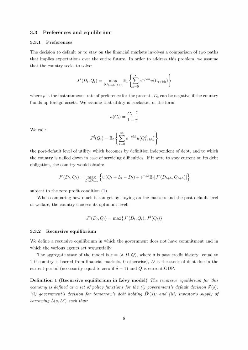
3.3 Preferences and equilibrium

3.3.1 Preferences

The decision to default or to stay on the financial markets involves a comparison of two paths

that implies expectations over the entire future. In order to address this problem, we assume

that the country seeks to solve:

J∗(Dt, Qt) = max{Ct+kh}k≥0

Et

{ ∞∑k=0

e−ρkhu(Ct+kh)

}

where ρ is the instantaneous rate of preference for the present. Dt can be negative if the country

builds up foreign assets. We assume that utility is isoelastic, of the form:

u(Ct) =C1−γt

1− γ

We call:

Jd(Qt) = Et

{ ∞∑k=0

e−ρkhu(Qdt+kh)

}the post-default level of utility, which becomes by definition independent of debt, and to which

the country is nailed down in case of servicing difficulties. If it were to stay current on its debt

obligation, the country would obtain:

Jr(Dt, Qt) = maxLt,Dt+h

{u (Qt + Lt −Dt) + e−ρhEt[J∗(Dt+h, Qt+h)]

}subject to the zero profit condition (1).

When comparing how much it can get by staying on the markets and the post-default level

of welfare, the country chooses its optimum level:

J∗(Dt, Qt) = max{Jr(Dt, Qt), Jd(Qt)}

3.3.2 Recursive equilibrium

We define a recursive equilibrium in which the government does not have commitment and in

which the various agents act sequentially.

The aggregate state of the model is s = (δ,D,Q), where δ is past credit history (equal to

1 if country is barred from financial markets, 0 otherwise), D is the stock of debt due in the

current period (necessarily equal to zero if δ = 1) and Q is current GDP.

Definition 1 (Recursive equilibrium in Levy model) The recursive equilibrium for this

economy is defined as a set of policy functions for the (i) government’s default decision δ′(s);

(ii) government’s decision for tomorrow’s debt holding D′(s); and (iii) investor’s supply of

borrowing L(s,D′) such that:

8

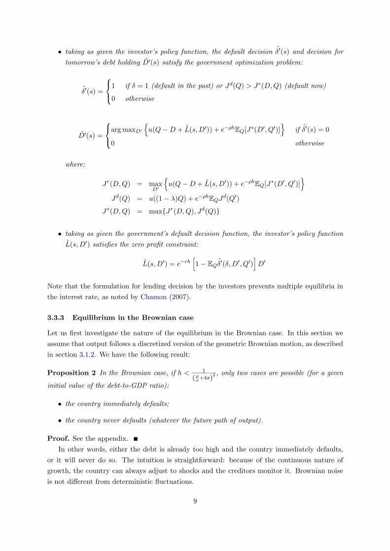
• taking as given the investor’s policy function, the default decision δ′(s) and decision for

tomorrow’s debt holding D′(s) satisfy the government optimization problem:

δ′(s) =

1 if δ = 1 (default in the past) or Jd(Q) > Jr(D,Q) (default now)

0 otherwise

D′(s) =

arg maxD′{u(Q−D + L(s,D′)) + e−ρhEQ[J∗(D′, Q′)]

}if δ′(s) = 0

0 otherwise

where:

Jr(D,Q) = maxD′

{u(Q−D + L(s,D′)) + e−ρhEQ[J∗(D′, Q′)]

}Jd(Q) = u((1− λ)Q) + e−ρhEQJd(Q′)

J∗(D,Q) = max{Jr(D,Q), Jd(Q)}

• taking as given the government’s default decision function, the investor’s policy function

L(s,D′) satisfies the zero profit constraint:

L(s,D′) = e−rh[1− EQδ′(δ,D′, Q′)

]D′

Note that the formulation for lending decision by the investors prevents multiple equilibria in

the interest rate, as noted by Chamon (2007).

3.3.3 Equilibrium in the Brownian case

Let us first investigate the nature of the equilibrium in the Brownian case. In this section we

assume that output follows a discretized version of the geometric Brownian motion, as described

in section 3.1.2. We have the following result:

Proposition 2 In the Brownian case, if h < 1

(µσ+4σ)2 , only two cases are possible (for a given

initial value of the debt-to-GDP ratio):

• the country immediately defaults;

• the country never defaults (whatever the future path of output).

Proof. See the appendix.

In other words, either the debt is already too high and the country immediately defaults,

or it will never do so. The intuition is straightforward: because of the continuous nature of

growth, the country can always adjust to shocks and the creditors monitor it. Brownian noise

is not different from deterministic fluctuations.

9

One empirical question that this result points to is whether, in the real world, decisions

are indeed taken continuously. The Greek case provides an instructive example. When Prime

Minister Papandreou took office, he realized that the deficit he inherited was much larger than he

originally thought. Having been given the wrong information in the beginning inevitably delayed

the right policy choices on his part. Perhaps, the lag in evaluating the situation is responsible

for the crisis. We return to this question in the empirical analysis that we submit below. One

can nevertheless compute the length of the time window h∗ during which a policymaker can

prevent crises triggered by Brownian shocks. For reasonable parameterizations of the model,

one has a time window of about one quarter (this would be roughly the case when µ/σ is near

one). For more volatile economies, say when µ = 2% and σ = 3% in quarterly frequency, the

time window is about 5 months. A paradox here is that the more volatile an economy is, the

more time a policymaker has to react to the shocks.

3.3.4 Equilibrium in the Poisson case

Let us now investigate the nature of the equilibrium in the Poisson case. In this section we

assume that output follows a discretized version of the geometric compound Poisson process,

as described in section 3.1.3. We arrive at the following result:

Proposition 3 In the Poisson case, the probability of default between dates t and t + 1 is

inferior to 1− e−p0.

Proof. By lemma 8, default never happens in the good state of nature. So the probability of

not having a default between dates t and t + h is superior to e−p0h. Therefore the probability

of not having a default between dates t and t+ 1 is superior to e−p0 (using the independence of

growth shocks between periods).

There are cases in which the probability of not having a default at each period is exactly

equal to e−p0 . Consider the extreme case where the country totally ignores the future (ρ = 0).

The default threshold (expressed as a debt-to-GDP ratio) is clearly d∗ = λ. Since, by lemma 8,

default never happens in the good state of nature, the country will always choose the maximum

debt level conditional to not defaulting in the good state (i.e. Dt+1 = λQt). This means that

the country will default in the bad state, and therefore the probability of default at each period

is equal to the probability of moving to the bad state: e−p0 .

The comparison between the Brownian and Poisson cases is straightforward. When the

economy is smooth, countries can continuously adjust their debt levels and never default. Ob-

viously, when the economy is disrupted by a Poisson shock, default becomes a possibility of

probability p0 (per unit of time).

3.3.5 Comparison with Aguiar and Gopinath (2006)

Aguiar and Gopinath (2006) suggested an interesting line of reasoning, which can be summarized

as follows: in emerging countries, growth rates (not output) are highly volatile. When growth

is expected to be high, this raises the willingness to borrow (as fast growth raises debt by

10

raising the permanent income) and therefore it also raises the risk of a debt overhang. Yet

the outcome is less satisfactory than expected as shown in Table 1: despite very high discount

factors, the debt levels remain quite low. Aguiar and Gopinath (2006) fail to recognize that the

volatility of the growth rate is not enough to trigger the risk of default; what is really needed

is a discontinuous jump in the parameters that switch the probability of default.

3.4 Numerical results

In order to get a better understanding of the properties of the models presented in this section,

we perform numerical exercises with calibrated versions of those models and analyze the sensi-

tivity of the results to the period duration h. Table 2 shows the calibration that we use for this

exercise.

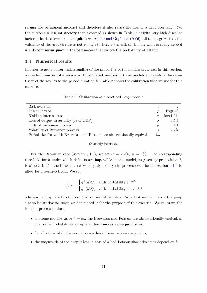
Table 2: Calibration of discretized Levy models

Risk aversion γ 2Discount rate ρ log(0.8)Riskless interest rate r log(1.01)Loss of output in autarky (% of GDP) λ 0.5%Drift of Brownian process µ 1%Volatility of Brownian process σ 2.2%Period size for which Brownian and Poisson are observationally equivalent h0 4

Quarterly frequency.

For the Brownian case (section 3.1.2), we set σ = 2.2%, µ = 1%. The corresponding

threshold for h under which defaults are impossible in this model, as given by proposition 2,

is h∗ ' 3.4. For the Poisson case, we slightly modify the process described in section 3.1.3 to

allow for a positive trend. We set:

Qt+h =

g+(h)Qt with probability e−p0h

g−(h)Qt with probability 1− e−p0h

where g+ and g− are functions of h which we define below. Note that we don’t allow the jump

size to be stochastic, since we don’t need it for the purpose of this exercise. We calibrate the

Poisson process so that:

• for some specific value h = h0, the Brownian and Poisson are observationally equivalent

(i.e. same probabilities for up and down moves, same jump sizes);

• for all values of h, the two processes have the same average growth;

• the magnitude of the output loss in case of a bad Poisson shock does not depend on h.

11

These constraints translate into the following relationships, which identify p0, g+(h) and g−(h):

e−p0h0 =1

2+

µ

2σ

√h0

∀h, e−p0hg+(h) + (1− e−p0h)g−(h) =

(1

2+

µ

2σ

√h

)eσ√h +

(1

2− µ

2σ

√h

)e−σ√h

∀h, g−(h)p0h

1− e−p0h= e−σ

√h0

p0h01− e−p0h0

Finally, the value chosen for h0 is one year.

Table 3 reports the results from the numerical simulations of these two models for various

values of h, which range approximately from one year to one week.

Table 3: Moments of discretized Levy processes for various period durations

Period duration (h, in quarters) 4 2 1 0.33

Discretized Brownian processDefault threshold (debt-to-GDP, quarterly, %) 48.4 51.9 68.8 79.3Default probability in 10 years (%) 35.7 0.0 0.0 0.0

Discretized Poisson processDefault threshold (debt-to-GDP, quarterly, %) 48.4 47.7 47.6 47.5Default probability in 10 years (%) 35.1 34.6 34.3 40.0

The processes are parametrized as described in section 3.4. The solution to the detrended model isapproximated using value function iteration on a grid of 25 points for the debt-to-GDP ratio. Momentsare obtained by averaging over 1,000 simulations of a length of 10 years.

One can see that proposition 2 is verified empirically: for h < h∗, the Brownian model has

zero default; conversely, the Poisson case still exhibits defaults as h goes to zero.

4 The full-fledged model

Building on the ideas presented in the previous section, we now construct a new model of

sovereign debt. It shares the core features of the model presented by Aguiar and Gopinath

(2006) and incorporates a few key ingredients which enable it to perform better with respect to

default frequency and average debt-to-GDP ratio.

4.1 The stochastic process

4.1.1 General form

We assume that the output of the country is described by the following stochastic process:

QtQt−1

= gt = eyt + zt

12

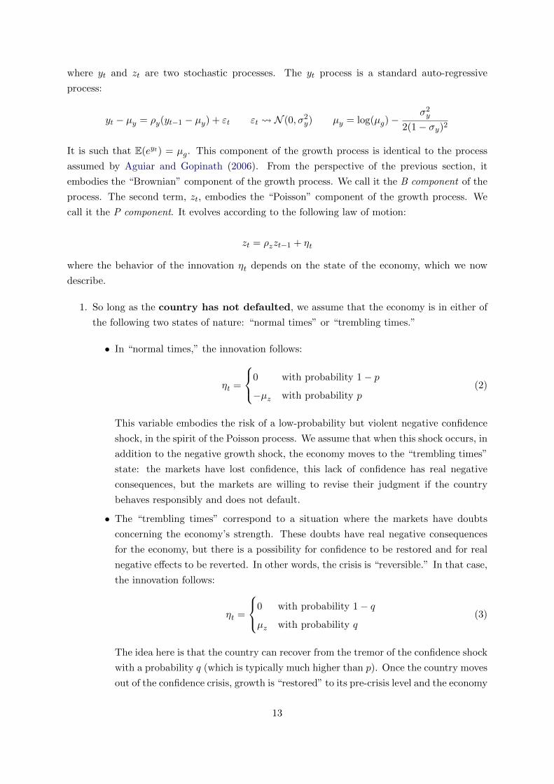
where yt and zt are two stochastic processes. The yt process is a standard auto-regressive

process:

yt − µy = ρy(yt−1 − µy) + εt εt N (0, σ2y) µy = log(µg)−σ2y

2(1− σy)2

It is such that E(eyt) = µg. This component of the growth process is identical to the process

assumed by Aguiar and Gopinath (2006). From the perspective of the previous section, it

embodies the “Brownian” component of the growth process. We call it the B component of the

process. The second term, zt, embodies the “Poisson” component of the growth process. We

call it the P component. It evolves according to the following law of motion:

zt = ρzzt−1 + ηt

where the behavior of the innovation ηt depends on the state of the economy, which we now

describe.

1. So long as the country has not defaulted, we assume that the economy is in either of

the following two states of nature: “normal times” or “trembling times.”

• In “normal times,” the innovation follows:

ηt =

0 with probability 1− p

−µz with probability p(2)

This variable embodies the risk of a low-probability but violent negative confidence

shock, in the spirit of the Poisson process. We assume that when this shock occurs, in

addition to the negative growth shock, the economy moves to the “trembling times”

state: the markets have lost confidence, this lack of confidence has real negative

consequences, but the markets are willing to revise their judgment if the country

behaves responsibly and does not default.

• The “trembling times” correspond to a situation where the markets have doubts

concerning the economy’s strength. These doubts have real negative consequences

for the economy, but there is a possibility for confidence to be restored and for real

negative effects to be reverted. In other words, the crisis is “reversible.” In that case,

the innovation follows:

ηt =

0 with probability 1− q

µz with probability q(3)

The idea here is that the country can recover from the tremor of the confidence shock

with a probability q (which is typically much higher than p). Once the country moves

out of the confidence crisis, growth is “restored” to its pre-crisis level and the economy

13

returns to “normal times.”

2. Following a default, the economy evolves as follows:

• If the country defaults during “normal times,” then the country suffers the same

negative growth shock that it would have undergone in case of a confidence crisis

(i.e. ηn+1 = −µz). However after default it remains in “normal times,” which means

that the output loss is not reversible (since the country has already defaulted).

• If the country defaults during “trembling times,” then it loses the ability to restore

output to pre-crisis levels. The country does not suffer an additional negative growth

shock (it has already undergone one), but the economy returns to “normal times,”

which means that it can no longer expect that positive news may end the crisis.

Since the country has defaulted, the doubts of the investors about the strength of

the economy have been confirmed and there is no reason to revert the shock.

In other words, a confidence shock acts like a “trembling hand” event: it shakes the economy

for a while. If during such an episode the country defaults, then the trembling shock becomes

permanent and no recovery takes place. When instead a country defaults while being in good

times, default creates on its own a confidence shock from which the economy does not recover

(except for the fact that the growth loss dies out naturally over time). The whole process is

summarized in Figure 1.

Figure 1: Law of motion of the economy

N is “normal times”, T is “trembling times”.

It should be noted here that the process assumed for the output shares some features with

the Markov-switching model for GDP introduced by Hamilton (1989). Like Hamilton’s, our

model has an underlying state variable corresponding to the current regime, and the mean of

the growth rate is different across regimes. But there are two critical differences. First, in

14

our model, the growth rate is only temporarily lowered in the “trembling” state, even if the

economy stays in that state for a long time (because zt is a mean reverting process), while in

Hamilton’s model, the growth rate is permanently lowered as long as the economy is in the bad

state. More importantly, the switch between the two regimes is partly endogenous in our model

(it can be triggered by a default decision), while it is entirely exogenous in Hamilton’s model.

4.2 The other costs of default

Beyond the output costs that we just described, a defaulting country is subject, as in the previous

models, to the following costs. First, creditors manage to inflict, on top of the trembling shock,

a penalty λ (which they do not monitor). Furthermore, they impose financial autarky on the

debtor, at least for a while, so that:

Cdt = Qdt = (1− λ)Qt

as long as the country is in default.

Following Arellano (2008) and others we assume that a defaulting country can return to

financial markets after a while. We call x the probability of a settlement at a given period.

When the settlement occurs, the penalty λ is lifted (but not the effect of the trembling shock).

Once a settlement is reached, debt is not canceled; it is only written down to a level consistent

with the post-default level of output and the historical data on post-default haircuts (see more

on this in section 4.4). We call V the settlement value of post default debt.

The pair (x, V ) (the duration of financial autarky after a default and the post-default recov-

ery value) have been modeled by Yue (2010) and Benjamin and Wright (2009) as the endogenous

outcome of a bargaining process following a default. Contrary to these authors, we assume that

the recovery value is not a function of past debt. The idea is simply that, after a default, prior

commitments become irrelevant.

Also note that if the recovery value V were too high (for example greater or equal to the debt

threshold above which the country defaults), then the resulting model would be conceptually

equivalent to a model where no settlement is ever reached after a default (i.e. where x = 0).6

4.3 The equilibrium

We define a recursive equilibrium in a similar fashion as in section 3.3.2. The government does

not make decisions under commitment, and the various agents act sequentially in response to a

state as defined below.

Definition 4 (State of the economy) The state of the economy is:

s = (δ, θ,D, y, z,Q)

6Note that in our framework the two options are not strictly equivalent because, in the case of a high V , thecountry will repeatedly pay the negative growth shock that occurs after a default. In the x = 0 case, the countrypays the negative growth shock only once.

15

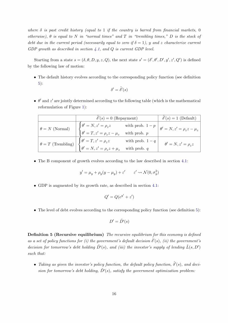
where δ is past credit history (equal to 1 if the country is barred from financial markets, 0

otherwise), θ is equal to N in “normal times” and T in “trembling times,” D is the stock of

debt due in the current period (necessarily equal to zero if δ = 1), y and z characterize current

GDP growth as described in section 4.1, and Q is current GDP level.

Starting from a state s = (δ, θ,D, y, z,Q), the next state s′ = (δ′, θ′, D′, y′, z′, Q′) is defined

by the following law of motion:

• The default history evolves according to the corresponding policy function (see definition

5):

δ′ = δ′(s)

• θ′ and z′ are jointly determined according to the following table (which is the mathematical

reformulation of Figure 1):

δ′(s) = 0 (Repayment) δ′(s) = 1 (Default)

θ = N (Normal)

θ′ = N, z′ = ρzz with prob. 1− p

θ′ = T, z′ = ρzz − µz with prob. pθ′ = N, z′ = ρzz − µz

θ = T (Trembling)

θ′ = T, z′ = ρzz with prob. 1− q

θ′ = N, z′ = ρzz + µz with prob. qθ′ = N, z′ = ρzz

• The B component of growth evolves according to the law described in section 4.1:

y′ = µy + ρy(y − µy) + ε′ ε′ N (0, σ2y)

• GDP is augmented by its growth rate, as described in section 4.1:

Q′ = Q(ey′+ z′)

• The level of debt evolves according to the corresponding policy function (see definition 5):

D′ = D′(s)

Definition 5 (Recursive equilibrium) The recursive equilibrium for this economy is defined

as a set of policy functions for (i) the government’s default decision δ′(s), (ii) the government’s

decision for tomorrow’s debt holding D′(s), and (iii) the investor’s supply of lending L(s,D′)

such that:

• Taking as given the investor’s policy function, the default policy function, δ′(s), and deci-

sion for tomorrow’s debt holding, D′(s), satisfy the government optimization problem:

16

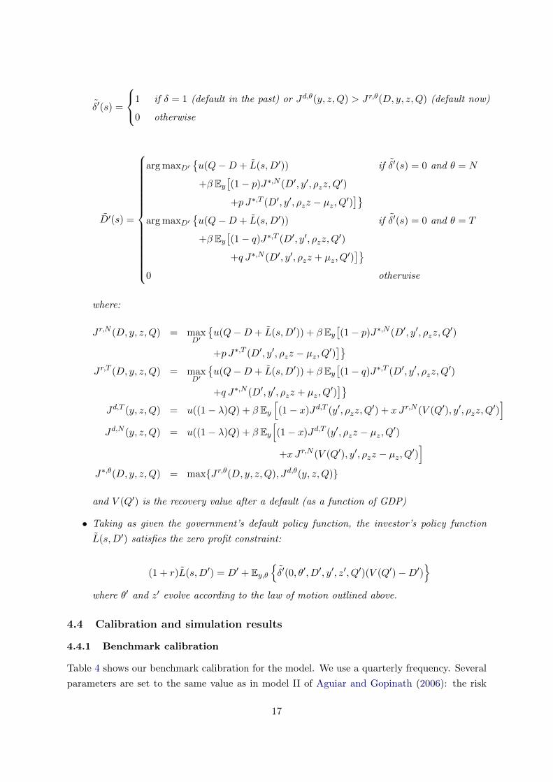
δ′(s) =

1 if δ = 1 (default in the past) or Jd,θ(y, z,Q) > Jr,θ(D, y, z,Q) (default now)

0 otherwise

D′(s) =

arg maxD′{u(Q−D + L(s,D′)) if δ′(s) = 0 and θ = N

+β Ey[(1− p)J∗,N (D′, y′, ρzz,Q

′)

+p J∗,T (D′, y′, ρzz − µz, Q′)]}

arg maxD′{u(Q−D + L(s,D′)) if δ′(s) = 0 and θ = T

+β Ey[(1− q)J∗,T (D′, y′, ρzz,Q

′)

+q J∗,N (D′, y′, ρzz + µz, Q′)]}

0 otherwise

where:

Jr,N (D, y, z,Q) = maxD′

{u(Q−D + L(s,D′)) + β Ey

[(1− p)J∗,N (D′, y′, ρzz,Q

′)

+p J∗,T (D′, y′, ρzz − µz, Q′)]}

Jr,T (D, y, z,Q) = maxD′

{u(Q−D + L(s,D′)) + β Ey

[(1− q)J∗,T (D′, y′, ρzz,Q

′)

+q J∗,N (D′, y′, ρzz + µz, Q′)]}

Jd,T (y, z,Q) = u((1− λ)Q) + β Ey[(1− x)Jd,T (y′, ρzz,Q

′) + xJr,N (V (Q′), y′, ρzz,Q′)]

Jd,N (y, z,Q) = u((1− λ)Q) + β Ey[(1− x)Jd,T (y′, ρzz − µz, Q′)

+xJr,N (V (Q′), y′, ρzz − µz, Q′)]

J∗,θ(D, y, z,Q) = max{Jr,θ(D, y, z,Q), Jd,θ(y, z,Q)}

and V (Q′) is the recovery value after a default (as a function of GDP)

• Taking as given the government’s default policy function, the investor’s policy function

L(s,D′) satisfies the zero profit constraint:

(1 + r)L(s,D′) = D′ + Ey,θ{δ′(0, θ′, D′, y′, z′, Q′)(V (Q′)−D′)

}where θ′ and z′ evolve according to the law of motion outlined above.

4.4 Calibration and simulation results

4.4.1 Benchmark calibration

Table 4 shows our benchmark calibration for the model. We use a quarterly frequency. Several

parameters are set to the same value as in model II of Aguiar and Gopinath (2006): the risk

17

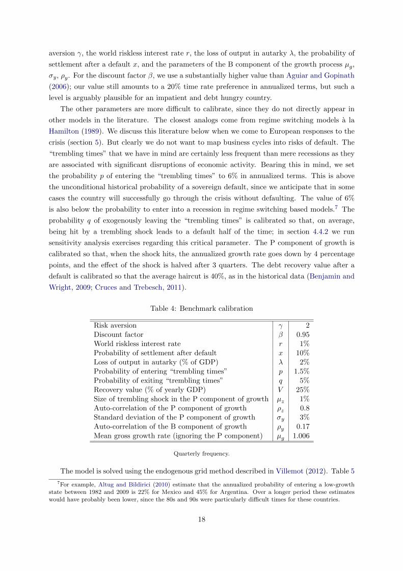
aversion γ, the world riskless interest rate r, the loss of output in autarky λ, the probability of

settlement after a default x, and the parameters of the B component of the growth process µg,

σy, ρy. For the discount factor β, we use a substantially higher value than Aguiar and Gopinath

(2006); our value still amounts to a 20% time rate preference in annualized terms, but such a

level is arguably plausible for an impatient and debt hungry country.

The other parameters are more difficult to calibrate, since they do not directly appear in

other models in the literature. The closest analogs come from regime switching models a la

Hamilton (1989). We discuss this literature below when we come to European responses to the

crisis (section 5). But clearly we do not want to map business cycles into risks of default. The

“trembling times” that we have in mind are certainly less frequent than mere recessions as they

are associated with significant disruptions of economic activity. Bearing this in mind, we set

the probability p of entering the “trembling times” to 6% in annualized terms. This is above

the unconditional historical probability of a sovereign default, since we anticipate that in some

cases the country will successfully go through the crisis without defaulting. The value of 6%

is also below the probability to enter into a recession in regime switching based models.7 The

probability q of exogenously leaving the “trembling times” is calibrated so that, on average,

being hit by a trembling shock leads to a default half of the time; in section 4.4.2 we run

sensitivity analysis exercises regarding this critical parameter. The P component of growth is

calibrated so that, when the shock hits, the annualized growth rate goes down by 4 percentage

points, and the effect of the shock is halved after 3 quarters. The debt recovery value after a

default is calibrated so that the average haircut is 40%, as in the historical data (Benjamin and

Wright, 2009; Cruces and Trebesch, 2011).

Table 4: Benchmark calibration

Risk aversion γ 2Discount factor β 0.95World riskless interest rate r 1%Probability of settlement after default x 10%Loss of output in autarky (% of GDP) λ 2%Probability of entering “trembling times” p 1.5%Probability of exiting “trembling times” q 5%Recovery value (% of yearly GDP) V 25%Size of trembling shock in the P component of growth µz 1%Auto-correlation of the P component of growth ρz 0.8Standard deviation of the P component of growth σy 3%Auto-correlation of the B component of growth ρy 0.17

Mean gross growth rate (ignoring the P component) µg 1.006

Quarterly frequency.

The model is solved using the endogenous grid method described in Villemot (2012). Table 5

7For example, Altug and Bildirici (2010) estimate that the annualized probability of entering a low-growthstate between 1982 and 2009 is 22% for Mexico and 45% for Argentina. Over a longer period these estimateswould have probably been lower, since the 80s and 90s were particularly difficult times for these countries.

18

reports the moments of the model simulated with the benchmark calibration. Like most models

in the quantitative sovereign debt literature, our model is able to replicate some important

stylized facts of the business cycle in emerging countries, such as a counter-cyclical current

account, counter-cyclical spreads and a more volatile consumption than output. But unlike

most models in the literature, it is able to sustain both a realistic frequency of defaults and a

realistic indebtment level (close to 40% of annual GDP).

Table 5: Moments of benchmark model

Benchmark With no Poisson (p = 0)

Rate of default (%, per year) 2.50 0.26Mean debt output ratio (%, annualized) 38.17 46.82σ(Q) (%) 4.45 4.42σ(C) (%) 6.04 6.89σ(TB/Q) (%) 2.63 3.47σ(Rs) (%) 0.57 0.18ρ(C,Q) 0.92 0.89ρ(TB/Q,Q) −0.41 −0.49ρ(Rs, Q) −0.60 −0.41ρ(Rs, TB/Q) 0.64 0.90

Parameters of the model are set to their benchmark values as in Table 4. The solution to the detrendedmodel is computed using the endogenous grid method described in Villemot (2012). The policyfunction are interpolated using a cubic spline on a 3-dimensional grid of 10 points for y, z and thedebt-to-GDP ratio. Moments are obtained by averaging over 500 simulated series of 1,500 points each,the first 1,000 of which are discarded. Q is GDP, C is consumption, TB/Q is trade balance over GDP,Rs is the spread. GDP, consumption, trade balance and spread are detrended with an HP filter ofparameter 1600.

In the last column of this table we also report the moments of the model when all parameters

are set to the benchmark calibration except for the probability p of a trembling shock coming

from the P component of growth, which is set to zero. One can see that in this configuration

defaults almost disappear. This shows the importance of the Poisson shock in this class of

models. As another consequence, the volatility of spreads almost goes to zero since there is

almost no risk of default.

4.4.2 Sensitivity analysis

We first investigate the sensitivity of the results to the probability q of exiting the “trembling

times.” As Figure 2 shows, three ranges appear. When q is high, no default ever takes place:

the trembling shock is expected to be short lived, the country will not destroy the recovery with

a default. At the other extreme, when q is low, the shock “pre-pays for the default.” Although

the country would not do it by on its own, the default now becomes the cheap option. In the

intermediate case, the choice being made depends on when and how the shock occurs. When the

economy is on a positive streak, default can be avoided, when instead the economy is already

down, then default becomes more palatable.

19

Figure 2: Default probability as a function of probability q of exiting the “trembling times”

0.05 0.10 0.15 0.20

12

34

5

Probability of getting out of the crisis state (q)

Def

ault

prob

abili

ty (

annu

al, %

)

Figure 3 shows the sensitivity of the mean debt-to-GDP ratio to the recovery value V of

the debt. The mean debt-to-GDP ratio is an increasing function of the recovery value: this was

to be expected since a higher recovery value means that default is more costly, and therefore a

higher level of debt can be sustained by the sovereign country. On this graph we also plot the

line corresponding to a fixed 40% haircut: one can see that the recovery level consistent with

this observed historical haircut is close to the 25% that we have chosen for our calibration.

4.4.3 A self-fulfilling re-interpretation

We show in this section that, when q is low enough, it is possible to reinterpret our model in the

spirit of self-fulfilling models pioneered by Cole and Kehoe (1996, 2000). Taking into account

the possibility of a self-fullfilling effect is important because, as shown by Cohen and Villemot

(2011), this effect plays a role in a significant minority of crises (around 20%).

In the cases when q is low enough, the trembling shock always triggers a default: this is so

because “the default is prepaid” through the crisis. A self-fulfilling reinterpretation becomes

possible, as outlined below.

Assume that markets fear a default anytime they see a sunspot. When markets starts

anticipating a default on their own, assume that they create a negative wave which is expected

to be long lasting, corresponding to low values of q. The country then defaults with probability

one. The shock is self-fulfilling. The difference with the model that we presented above is

that, in the self-fulfilling interpretation, the shock is triggered because of the fear of a default

20

Figure 3: Mean debt-to-GDP as a function of recovery value

10 20 30 40 50

2530

3540

4550

55

Recovery (% of annual GDP)

Deb

t/GD

P (

annu

al, %

)

The dotted line indicates the debt-to-GDP value corresponding to a 40% haircut.

rather than for reasons independent of the fear of default. But for low values of q the two are

observationally equivalent.

5 Eurozone policies

5.1 Analysis at business cycle frequencies

As we already mentionned, our modelling strategy for the output process is close to that of

Hamilton (1989). Let us now see what the consequences would be of plugging the parameter

values estimated by the Markov-switching literature into our model.

The original model of Hamilton (1989) estimated on US data for the period 1952–1984

gives p = 9.5% and q = 24.5%. Later, Goodwin (1993) has estimated a similar model on 8

advanced economies from the late 1950s/early 1960s to the late 1990s, and came up with values

for p ranging from 1% to 9%, and for q ranging from 21% to 49%.8 Table 6 reports default

probabilities and mean debt-to-GDP ratios obtained with the model of section 4 for values of p

and q lying in the estimated range for business cycles of advanced countries.

As we can see from this table, the most prominent fact exhibited by this exercise is that the

risk of default at business cycle frequencies of advanced economies is negligible. The trembling

times that we are talking about are therefore events which are less frequent and more severe

8We disregard the result for Italy, since the author labels it a pathological case and explains that a 3-statespecification would probably better fit the data for that country.

21

Table 6: Model simulations using business cycle frequencies in advanced economies

Probability of entering “trembling times” (p, per quarter) 1% 1% 10% 10%Probability of exiting “trembling times” (q, per quarter) 20% 50% 20% 50%

Rate of default (per year) 0.38% 0.27% 0.32% 0.29%Mean debt output ratio (annualized) 45% 47% 43% 46%

The simulations are done using the model presented in section 4. The values tested for p and qcorrespond approximately to the extreme values estimated by Hamilton (1989) and Goodwin (1993)on 7 advanced economies over the postwar period. Other parameters of the model are set to theirbenchmark values as in Table 4.

downturns than business cycles downturns (such as a banking crises or a very severe recession).

This is why we chose parameter values such that crises are less frequent (lower p) and longer

lasting (lower q) than mere recessions.

5.2 Credit ceilings

Following the Greek crisis, the eurozone imposed a new set of stringent rules to avoid future

crises. The idea of policymakers is to impose a tougher credit ceiling on eurozone countries

in order to protect the zone from any risk of default. The following questions are therefore of

major importance from a policy perspective: how low should the debt ceilings be to avert any

risk of crisis? What are the welfare implications of these constraints?

In order to address these questions, we have computed the levels of debt that are consistent

with no default in either “normal” or “trembling” times in our model. Figure 4 summarizes

the results as a function of the key parameter q. The solid line represents the mean debt-to-

GDP ratio, the dotted line represents the maximum debt-to-GDP level under which there is

no default in “normal times,” and the dashed line represents the maximum debt-to-GDP level

under which there is no default in “trembling times.”

It is interesting to note that, for values of q less than 5%, the mean debt-to-GDP ratio is a

decreasing function of q; the country becomes less prudent and is willing to take on more debt

as the risk of default becomes higher because it knows that it will not repay its debt in bad

states of nature. This is the “Panglossian effect” described in Cohen and Villemot (2011).

One should also note that the proper way to introduce a relevant credit ceiling is to allow for

two different levels: one pertaining to “normal times” and one pertaining to “trembling times.”

Imposing one only ceiling for both states of nature would be quite an inefficient way to avoid

default. Extraordinary times call at extraordinary debt ceilings. This is a key distinction that

tends to be lost in current policy debates.

Figure 4 shows, as expected, that debt ceilings to avoid default are an increasing function

of the parameter q. For a short-lived crisis episode (q around 20%), countries take care of

themselves as they do not default and are able to stabilize their debt. Thus, no debt ceiling is

needed in this situation. This is in line with the business cycle properties that we examined in

section 5.1.

22

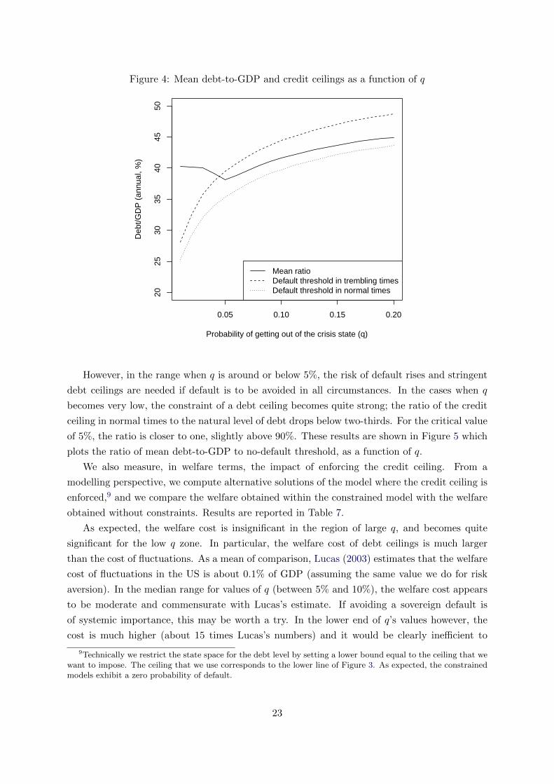
Figure 4: Mean debt-to-GDP and credit ceilings as a function of q

0.05 0.10 0.15 0.20

2025

3035

4045

50

Probability of getting out of the crisis state (q)

Deb

t/GD

P (

annu

al, %

)

Mean ratioDefault threshold in trembling timesDefault threshold in normal times

However, in the range when q is around or below 5%, the risk of default rises and stringent

debt ceilings are needed if default is to be avoided in all circumstances. In the cases when q

becomes very low, the constraint of a debt ceiling becomes quite strong; the ratio of the credit

ceiling in normal times to the natural level of debt drops below two-thirds. For the critical value

of 5%, the ratio is closer to one, slightly above 90%. These results are shown in Figure 5 which

plots the ratio of mean debt-to-GDP to no-default threshold, as a function of q.

We also measure, in welfare terms, the impact of enforcing the credit ceiling. From a

modelling perspective, we compute alternative solutions of the model where the credit ceiling is

enforced,9 and we compare the welfare obtained within the constrained model with the welfare

obtained without constraints. Results are reported in Table 7.

As expected, the welfare cost is insignificant in the region of large q, and becomes quite

significant for the low q zone. In particular, the welfare cost of debt ceilings is much larger

than the cost of fluctuations. As a mean of comparison, Lucas (2003) estimates that the welfare

cost of fluctuations in the US is about 0.1% of GDP (assuming the same value we do for risk

aversion). In the median range for values of q (between 5% and 10%), the welfare cost appears

to be moderate and commensurate with Lucas’s estimate. If avoiding a sovereign default is

of systemic importance, this may be worth a try. In the lower end of q’s values however, the

cost is much higher (about 15 times Lucas’s numbers) and it would be clearly inefficient to

9Technically we restrict the state space for the debt level by setting a lower bound equal to the ceiling that wewant to impose. The ceiling that we use corresponds to the lower line of Figure 3. As expected, the constrainedmodels exhibit a zero probability of default.

23

Figure 5: Credit ceilings as a fraction of equilibrium levels in normal times

0.05 0.10 0.15 0.20

0.65

0.70

0.75

0.80

0.85

0.90

0.95

Probability of getting out of the crisis state (q)

Rat

io o

f mea

n de

bt−

to−

GD

P to

no−

defa

ult t

hres

old

This graph shows the ratio of the credit ceiling to avoid default (in “normal times”) to the meandebt-to-GDP ratio, as presented on Figure 4.

Table 7: Welfare cost of imposing credit ceilings

Probability of exiting “trembling times” (q, per quarter) 1% 5% 10% 20%

Unconstrained welfare −18.273 −18.510 −18.524 −18.570Constrained welfare −18.573 −18.581 −18.578 −18.573

Cost of ceiling (permanent loss of GDP) 1.64% 0.39% 0.30% 0.02%

Welfare is computed in both models for a level of debt equal to the ceiling, and at the mean productivitylevel (y = µy, z = 0) and in “normal times” (θ = N). The cost of imposing the ceiling as a percentageof GDP is computed using a Lucas (1987) type calculation; we first consider an economy with the

same preferences but no fluctuations(i.e. an economy where the welfare is W = u((1−∆)Q)

1−β

), and

then we report the value of ∆ that generates the same drop in welfare as the one observed betweenthe unconstrained and constrained economies reported in the table.

24

target a zero default equilibrium. In our simulations, we picked a 5% value for q, for which the

constrained equilibrium remains reasonably close to the unconstrained one.

5.3 Further insights

When investigating the policy implications of our model for the eurozone, we did not modify

the value of the parameter governing the magnitude of the trembling shock (µz) from the

value set for the emerging country benchmark; we left it at 1 percentage point of the GDP

growth rate. Quantitatively, this means that following a trembling shock, the GDP level will

be permanently lowered by 3.8% relative to the pre-shock trend.10 This is a sizable shock,

but not so big compared to what Greece is currently undergoing.11 When it comes to the

eurozone, it could therefore make sense to use greater values for the magnitude of the trembling

shock, and for the two other parameters governing the cost of default (the direct penalty on

output λ and the recovery value V ).12 This would reflect the fact that in a monetary union

with a highly integrated banking system, eurozone countries face a higher cost for default. For

example, if we increase these three parameters by a factor of 1.5 (i.e. µz = 0.015, λ = 3%

and V = 37.5% of GDP), and with other parameters being held at the benchmark values given

in Table 4, the mean debt-to-GDP ratio jumps to 58.8% (which is an increase by a factor of

1.5 compared to the benchmark case given in Table 5). Only the default frequency remains

relatively unchanged at 2.4%. Our model is therefore capable of delivering an arbitrarily high

level of debt-to-GDP through a homothetic re-scaling of the three parameters µz, λ and V ,

while keeping the default probabilities at a constant level.

Another point worth mentioning is that in the framework under which the eurozone operates,

up to 50% of public debt is held by foreigners. In fact the three countries which have been most

vulnerable to the recent crisis (Greece, Portugal and Ireland) all had more than 70% of their

public debt held by foreigners. A straightforward policy lesson to avoid default risk on sovereign

issuers could be to make sure that sovereign debt is primarily held by domestic institutions or

individuals, as is the case in Japan for instance. Of course, for a given path of current accounts,

this would imply that other (private) debt would be held outside the country. This is irrelevant

in our model, since we don’t distinguish between public and private external debt.13 However,

10If gt is the growth rate without trembling shock, and gt is the growth rate following a trembling shock att = 0, then the long-term ratio of the two corresponding GDP levels is:∏+∞

t=0 gt∏+∞t=0 gt

=

+∞∏t=0

(1 +

ρtzµzeµy

)' 0.962

11According to some estimates, Greece GDP level could be more than 10% below its pre-crisis trend.12Note that the size of the trembling shock µz influences the cost of default, because upon default the country

loses the possibility of having its output restored to the pre-crisis level; since the size of the output restorationdepends on µz as shown in (3), so does the cost of default. If we were to distinguish the size of the tremblingshock in (2) from the size of the restoration in (3), then only the latter would have an impact on the default cost.

13The rationale for not distinguishing between public and private debt is that private external loans generallycome with an explicit or implicit public guarantee, as documented by Reinhart and Rogoff (2011). This isconfirmed by a positive correlation between sovereign default and access of the private sector to foreign credit,as documented by Arteta and Hale (2008). These considerations have led Mendoza and Yue (2011) to present amodel where private and public external debt bear the same interest rate spread and the same credit risk.

25

in a more thoughtful model where the distinction is introduced, this could have interesting

policy implications.

6 Conclusion

We have analyzed a model in which countries usually do not like to default, but rather are

forced into default when the economy turns sour, arguing that this modelling choice better fits

the historical reality. Based on this postulate, the key message of the paper is simply that in

order to avoid default, the critical parameter to analyze is the speed at which economies can

move out of these “trembling times” (the parameter q in our model). Clearly, this is a lesson

that European policymakers should understand, as the more protracted the economic crisis

(and, hence, the perception that countries entering into “trembling times” will stay there for a

while), the higher the risk of default. In the worst case scenario when a crisis is expected to

be very long lasting, the debt ceiling needed to avoid default may become very low. Building

institutions that avoid default risk should not only rely on debt ceilings, but also on mechanisms

that limit the duration of the “trembling times.” One key distinction between advanced and

poor countries is the supposedly superior ability of advanced economies to recover from crisis

(rather than sheer recessions), as documented by Hausmann et al. (2006). The mess created

in Europe by the management of the sovereign crisis has certainly shifted the perception of

the European ability to exit “trembling times,” making the risk of a default much higher for

all sovereigns within the eurozone. This is where the debate on the macro-management of the

crisis would certainly need to be addressed. Reassuring investors of the policymakers’ ability

to address trembling episodes is perhaps more important than imposing credit ceilings that are

too stringent.

References

Aguiar, M. and G. Gopinath (2006): “Defaultable debt, interest rates and the current

account,” Journal of International Economics, 69, 64–83.

Altug, S. G. and M. Bildirici (2010): “Business Cycles around the Globe: A Regime-

switching Approach,” CEPR Discussion Papers 7968, C.E.P.R. Discussion Papers.

Applebaum, D. (2004): Levy Processes and Stochastic Calculus, Cambridge studies in ad-

vanced mathematics, Cambridge University Press, second ed.

Arellano, C. (2008): “Default Risk and Income Fluctuations in Emerging Economies,” The

American Economic Review, 98, 690–712.

Arteta, C. and G. Hale (2008): “Sovereign debt crises and credit to the private sector,”

Journal of International Economics, 74, 53–69.

26

Benjamin, D. and M. L. J. Wright (2009): “Recovery Before Redemption: A Theory

Of Delays In Sovereign Debt Renegotiations,” CAMA Working Papers 2009-15, Australian

National University, Centre for Applied Macroeconomic Analysis.

Bulow, J. and K. Rogoff (1989): “A Constant Recontracting Model of Sovereign Debt,”

Journal of Political Economy, 97, 155–78.

Chamon, M. (2007): “Can debt crises be self-fulfilling?” Journal of Development Economics,

82, 234–244.

Chatterjee, S. and B. Eyigungor (2011): “Maturity, indebtedness, and default risk,”

Working Papers 11-33, Federal Reserve Bank of Philadelphia.

Cohen, D. (1992): “The Debt Crisis: A Postmortem,” in NBER Macroeconomics Annual

1992, Volume 7, National Bureau of Economic Research, Inc, NBER Chapters, 65–114.

Cohen, D. and J. Sachs (1986): “Growth and external debt under risk of debt repudiation,”

European Economic Review, 30, 529–560.

Cohen, D. and C. Valadier (2011): “40 years of sovereign debt crises,” CEPR Discussion

Papers 8269, Centre for Economic Policy and Research.

Cohen, D. and S. Villemot (2011): “Endogenous debt crises,” CEPR Discussion Papers

8270, Centre for Economic Policy and Research.

Cole, H. L. and T. J. Kehoe (1996): “A self-fulfilling model of Mexico’s 1994–1995 debt

crisis,” Journal of International Economics, 41, 309–330.

——— (2000): “Self-Fulfilling Debt Crises,” Review of Economic Studies, 67, 91–116.

Cruces, J. J. and C. Trebesch (2011): “Sovereign Defaults: The Price of Haircuts,” CESifo

Working Paper Series 3604, CESifo Group Munich.

Cuadra, G. and H. Sapriza (2008): “Sovereign default, interest rates and political uncer-

tainty in emerging markets,” Journal of International Economics, 76, 78–88.

Eaton, J. and M. Gersovitz (1981): “Debt with Potential Repudiation: Theoretical and

Empirical Analysis,” Review of Economic Studies, 48, 289–309.

Fink, F. and A. Scholl (2011): “A Quantitative Model of Sovereign Debt, Bailouts and Con-

ditionality,” Working Paper Series of the Department of Economics, University of Konstanz

2011-46, Department of Economics, University of Konstanz.

Goodwin, T. H. (1993): “Business-Cycle Analysis with a Markov-Switching Model,” Journal

of Business & Economic Statistics, 11, 331–39.

Hamilton, J. D. (1989): “A New Approach to the Economic Analysis of Nonstationary Time

Series and the Business Cycle,” Econometrica, 57, 357–84.

27

Hatchondo, J. C. and L. Martinez (2009): “Long-duration bonds and sovereign defaults,”

Journal of International Economics, 79, 117–125.

Hatchondo, J. C., L. Martinez, and H. Sapriza (2010): “Quantitative properties of

sovereign default models: solution methods,” Review of Economic Dynamics, 13, 919–933.

Hausmann, R., F. Rodriguez, and R. Wagner (2006): “Growth Collapses,” Working

Paper Series rwp06-046, Harvard University, John F. Kennedy School of Government.

Inter-American Development Bank (2007): Living with Debt: How to Limit Risks of

Sovereign Finance, Economic and Social Progress Report (IPES), IADB.

Levy-Yeyati, E. and U. Panizza (2011): “The elusive costs of sovereign defaults,” Journal

of Development Economics, 94, 95–105.

Lucas, R. E. (1987): Models of business cycles, Basil Blackwell.

——— (2003): “Macroeconomic Priorities,” American Economic Review, 93, 1–14.

Mendoza, E. G. and V. Z. Yue (2011): “A General Equilibrium Model of Sovereign Default

and Business Cycles,” NBER Working Papers 17151, National Bureau of Economic Research,

Inc.

Reinhart, C. M. and K. S. Rogoff (2009): This Time is Different, Princeton University

Press.

——— (2011): “From Financial Crash to Debt Crisis,” American Economic Review, 101, 1676–

1706.

Reinhart, C. M., K. S. Rogoff, and M. A. Savastano (2003): “Debt Intolerance,”

Brookings Papers on Economic Activity, 34, 1–74.

Rogoff, K. S. (2011): “Sovereign Debt in the Second Great Contraction: Is This Time

Different?” NBER Reporter, 3, 1–5.

Sturzenegger, F. and J. Zettelmeyer (2007): Debt Defaults and Lessons from a Decade

of Crises, MIT Press Books, The MIT Press.

Villemot, S. (2012): “Solving sovereign debt models faster: an endogenous grid method,”

Dynare working paper (forthcoming), CEPREMAP.

World Bank (2004): World Development Indicators 2004, World Bank.

——— (2010): Global Development Finance 2011: External Debt of Developing Countries,

World Bank.

Yue, V. Z. (2010): “Sovereign default and debt renegotiation,” Journal of International Eco-

nomics, 80, 176–187.

28

A Extra results and proofs

A.1 General case

Proposition 6 (Eaton and Gersovitz (1981)) Default incentives are stronger the higher

the debt

Proposition 7 Default occurs if and only if debt-to-GDP ratio is higher than a given threshold

d∗.

Proof. This is a straightforward implication of the isoelasticity of preferences and of the

Markovian nature of the stochastic process driving output and recovery.

A.2 Brownian or Poisson case

In this section we establish a lemma valid for both the Brownian case (section 3.1.2) and the

Poisson case (section 3.1.3).

Lemma 8 For both the Brownian and the Poisson cases, the country never chooses an indebt-

ment level such that default is sure tomorrow (i.e. a level for which L′(s, D′(s)) = 0).

Proof. By contradiction.

We denote by g+ the growth rate in the good case and g− in the bad case,14 and p is the

probability of a being in the bad case.

Suppose that for some state s, the optimal choice is to repay and have L′(s, D′(s)) = 0.

Since it means that default is sure tomorrow, we have:

d∗ <D′(s)

g+Q

We also have:

Jr(s) = u(Q−D) + (1− p)e−ρhJd(g+Q) + p e−ρhJd(g−Q)

Now let D′2 = d∗g−Q. It is clear that this level of indebtment is in the safe zone, so that

L(s,D′2) = e−rhD′2. If the country was choosing that level of indebtment, it would get:

Jr2 (s) = u(Q−D + e−rhD′2) + (1− p)e−ρhJr(D′2, g+Q) + p e−ρhJr(D′2, g−Q)

But since Jr(D′2, g+Q) ≥ Jd(g+Q) and Jr(D′2, g

−Q) ≥ Jd(g−Q) by construction of D′2, we

therefore have:

Jr2 (s) > Jr(s)

14In the Poisson case, g− can actually be a random variable (see section 3.1.3). The demonstration still appliesin this case, with the following modifications:

• in the definition of D′2, replace g− by the minimum value that growth can take in the case of a bad shock;

• add conditional expectation operators in the last terms defining Jr(s) and Jr2 (s).

29

This is in contradiction with the optimality of D′(s).

A.3 Brownian case

In this section, we denote by p the probability that output is low tomorrow, i.e. p = 12 −

µ2σ

√h.

In order to demonstrate proposition 2, we begin by establishing the following lemma:

Lemma 9 In the Brownian case, if h ≤ 1

(4σ+µσ )

2 , the risky interest rate (r + p in first approx-

imation) does not happen in equilibrium.

Proof. By contraposition. Assume that for some state s, the optimal choice is to repay and

L(s, D′(s)) is equal to e−rh(1− p)D′(s): this is the risky case where the country will repay next

period in the good state of nature, but default in the bad state (the other two possible values

for L(s, D′(s)) are e−rhD′(s) and 0, since output can take only two values). This implies that:

D′(s)

eσ√hQ≤ d∗ < D′(s)

e−σ√hQ

We also have:

Jr(s) = u(Q−D + e−rh(1− p)D′(s)) + (1− p)e−ρhJr(D′(s), eσ√hQ) + p e−ρhJd(e−σ

√hQ)

Let D′2 = e−2σ√hD′(s). We therefore have

D′2e−σ√hQ≤ d∗, which means that this level of indebt-

ment is in the safe zone, and that L(s,D′2) = e−rhD′2. If the country was choosing that level of

indebtment, it would get:

Jr2 (s) = u(Q−D + e−rhD′2) + (1− p)e−ρhJr(D′2, eσ√hQ) + p e−ρhJr(D′2, e

−σ√hQ)

By optimality of D′(s), we have Jr(s) > Jr2 (s). And since we have Jr(D′2, eσ√hQ) > Jr(D′(s), eσ

√hQ)

(by proposition 6) and Jr(D′2, e−σ√hQ) > Jd(e−σ

√hQ) (by construction of D′2), this implies that

u(Q−D+ e−rh(1− p)D′(s)) > u(Q−D+ e−rhD′2). In turn, this implies that (1− p) > e−2σ√h,

or ln(1 − p) > −2σ√h. Using the concavity of the logarithm, this implies p < 2σ

√h, which is

equivalent to h > 1

(4σ+µσ )

2 .

Intuitively, when h is small, then the variance of next period output conditionally to today’s

output is small. The country will prefer to borrow a little less, in order to be in the safe zone,

since the effort to be done is small and tends towards zero, while the cost of a default remains

high.

Proof of proposition 2. Assume that the country decides to repay. Given that next period

output can take only two values, three cases are possible for tomorrow:

1. the country will repay in both states,

2. the country will repay in the good state of nature and default in the bad state,

3. the country will default in both states.

30

The second and third cases are excluded by lemmas 8 and 9.

By forward recursion, it is clear that the country will always repay in the future.

31