DETERMINANTS OF MULTIFAMILY

MORTGAGE DEFAULT

By

Wayne R. ArcherPeter J. Elmer

David M. Harrisonand

David C. Ling

June, 1999

Working Paper 99-2(Electronic copies of FDIC Working Papers are available at www.fdic.gov)

Federal Deposit Insurance Corporation

DETERMINANTS OF MULTIFAMILY MORTGAGE DEFAULT

Wayne R. ArcherCenter for Real Estate Studies

Department of Finance, Insurance & Real EstateUniversity of Florida

Peter J. ElmerDivision of Research and Statistics

Federal Deposit Insurance Corporation

David M. HarrisonSchool of Business Administration

University of Vermont

David C. Ling*Center for Real Estate Studies

Department of Finance, Insurance & Real EstateUniversity of Florida

Abstract

Option-based models of mortgage default posit that the central measure of default risk is the loan-to-value (LTV) ratio. We argue, however, that an unrecognized problem with extending the basicoption model to existing multifamily and commercial mortgages is that key variables in the optionmodel are endogenous to the loan origination and property sale process. This endogeneity implies,among other things, that no empirical relation may be observed between default and LTV. Thisis because lenders may require lower LTVs in order to mitigate risk, so mortgages with low andmoderate LTVs may be as likely to default as those with high LTVs. Mindful of this riskendogeneity and its empirical implications, we examine the default experience of 9,639multifamily mortgage loans securitized by the Resolution Trust Corporation (RTC) and theFederal Deposit Insurance Corporation (FDIC) during the period 1991!1996. The extensivenature of the data supports multivariate analysis of default incidence in a number of respects notpossible in previous studies.

* The views expressed in this paper are those of the authors and not necessarily those of theFederal Deposit Insurance Corporation. Correspondence may be directed either to Center forReal Estate Studies, Department of Finance, Insurance & Real Estate, University of Florida,Gainesville, FL 32611-7168. Phone: (352) 392-9307, Fax: (352) 392-0301, E-mail:ling@dale.cba.ufl.edu or to Peter Elmer, FDIC Division of Research and Statistics, 550 17th St.N.W., Washington, D.C. 20429. Phone: (202) 898-7366, Fax: (202) 898-7189, E-mail:pelmer@fdic.gov.

1Bradley, Nothaft, and Freund (1998) show that the share of multifamily mortgages heldby life insurance companies and pension funds declined steadily from 17.8 percent in 1980 to 9.0percent in 1997. The largest recent growth occurred in the private-label commercial mortgagesecurity sector, which jumped from 0 to over 12 percent between 1990 and 1997. The FreddieMac and Fannie Mae share rose from 10.5 to 12.3 percent between 1990 and 1997. Banks andsavings institutions maintained the largest share, although their share fell from 50.5 percent in1980 to 33.8 percent in 1997.

DETERMINANTS OF MULTIFAMILY MORTGAGE DEFAULT

1. INTRODUCTION

Default of commercial mortgage loans during the last decade has been a significant

investment risk. The collective evidence suggests that default may occur with over 15 percent of

commercial (income-producing property) loans (Snyderman [1994]) and that the resultant yield

degradation, given foreclosure, may approach 1,000 basis points (Ciochetti [1998]). Although many

partial bodies of data attest to this default risk, available sources have revealed only very limited

views of the problem. Early studies rely primarily on the foreclosure experience of major life

insurance companies. However, although this experience is important, insurance companies

represent less than one-fifth of the multifamily investor market and the analysis focuses on only one

form of commercial mortgage default (foreclosure).1 Recent work examines the experience of other

investors in the same activity class as life insurance companies, such as Freddie Mac and Fannie Mae

(Goldberg and Capone [1998]) and FHA (Follain et al. [1999]), and also focuses on restricted

definitions of default.

This paper examines the determinants of multifamily mortgage default for the largest class of

multifamily originators and investors, banks and savings institutions, using a broad definition of

default that recognizes all types of default-related events, such as loan modifications and workouts as

2Snyderman (1994) reports a variety of default-related data from all types of commercialmortgages held by life insurance companies, 10!20 percent of which are multifamily. Vandell etal. (1993) and Episcopos et al. (1998) distinguish multifamily loans from other types ofcommercial mortgages, but only in the context of a general model of commercial mortgagedefault. Interestingly, these two studies consistently find multifamily to be one of the strongestproperty-type variables in their default analysis.

3 Although conduit loans are generally “thrift” quality, Quigg (1998) argues that theydiffer from our RTC/FDIC loans in that they are originated with more recent underwritingstandards and are subject to the scrutiny of rating agencies and investors.

4 Fitch (1996) provides a practitioner analysis of multifamily and commercial loans thatincludes portions of the data covered by our analysis. Unfortunately, all of the analyses in theFitch report were done by looking at the effects of a single variable on default and losses (that is, univariate regressions). For a thorough discussion of the drawbacks of the Fitch report, seeQuigg (1997).

well as foreclosures.2 We examine the default experience of multifamily mortgages found in 22 pools

of loans securitized by the RTC and the FDIC during the 1991!1996 period. These pools contain

mortgages of all sizes located in almost every state and originated by many institutions. As a result,

these RTC/FDIC loans may be closer than life insurance loans to the quality of typical conduit loans.3

The loan-level data contain extensive property, loan, and underwriting data, plus a record of loan

performance over time. The loans are also unique by virtue of the fact that most are believed to have

been held as portfolio investments by the originating institution. Interestingly, the overall default rate

of our sample is 17.5 percent, which is not significantly different from the default frequencies

reported for the loan portfolios of major life insurance companies over similar time periods.4 The

extensive nature of the data supports multivariate analysis of default in a number of respects not

possible in previous studies.

In formulating our empirical model, we look for guidance to option-based models of

commercial mortgage default. Although these models clearly suggest LTV and related factors as

central to the default “story,” their meaning fails to transfer to the case of multifamily mortgages.

We hypothesize that option-based models encounter problems in the commercial mortgage arena

because they fail to recognize key variables as endogenously affected by the loan origination process.

In particular, rational lenders will react to higher risk by setting LTV to offset or mitigate the risk.

Moreover, the observed “value” may vary with the availability and/or terms of the financing. These

endogenous elements imply that no empirical relationship may be found between default and LTV.

Overall, our results strongly suggest that the borrower’s ability to service the debt, or debt coverage

ratio (DCR), is more important in explaining default than LTV---a result inconsistent with the

predictions of option-based models.

In addition to examining the role of LTV and DCR, we also estimate the effects of property

characteristics, originating institution, and location on the incidence of default. The general finding is

that a limited explanatory role is played by each of these characteristics. For example, one of our

four property characteristics (number of units) is significant along with several location and lender

control variables. However, since many similar control variables have little explanatory power,

default rates appear more closely related to the characteristics of the loans than to those of the

property, originator, or location. Although the extent to which our results can be generalized

remains an open question, our findings contribute to the sparse collection of evidence on the

determinants of multifamily mortgage default.

In Section 2, we summarize the results of several previous default studies and clarify the

various phases of default experience that they represent. Section 3 discusses mortgage default in the

context of option theoretic models while exploring complications introduced when key elements of

those models are endogenously determined. The pervasive problem of censuring is also addressed.

In Section 4, we describe the RTC/FDIC data and compare them with other data that have been

studied. A logistic regression model is specified and estimated in Section 5, while a number of

5 However, he expands to 14 companies and updates the data to 1995.

robustness checks are detailed in Section 6. Section 7 summarizes the results, and concludes.

2. EXISTING EMPIRICAL STUDIES

Empirical analysis of commercial mortgage default is limited to a handful of studies. Two

important characteristics of existing studies are the sample source and the point in the process of

default that is the focus of the study. The significance of the latter issue is highlighted in figure 1.

Clearly, the “default rate” indicated by data can depend on how early in the process the point of

“default” is chosen. This is particularly important, as the diagram suggests, because various studies

have focused on different points in the default process.

Of the two components of the default problem, incidence and loss severity, studies have

tended to focus on one or the other. Two benchmark analyses rely on data from life insurance

company annual statements to regulators. Snyderman (1994) examines both the incidence of default

and loss severity using all individually reported commercial mortgage loans of eight large life

insurance companies originated from 1972 through 1986, as reported in 1991 annual statements.

The commercial mortgages in this study represented roughly 25 percent of the commercial

mortgages held by life insurance companies, and approximately 5 percent of all commercial

mortgages. The default rates from these data are potentially affected by size bias (all loans are $1

million or greater) and by censuring, and have no control for property type.

Ciochetti (1997) looks at loss severity using the same data source as the Snyderman study.5

He examines only foreclosed loans, estimating the loss recovery through the point when a loan is

transferred to REO (real estate owned). Ciochetti’s data set is slightly more comprehensive (loans

down to $500,000 and taken from 14 companies). This gives coverage of roughly 30 percent of life

6 Data are from various quarterly Investment Bulletins of the American Council of LifeInsurance.

insurance company commercial loans and approximately 6 percent of all commercial mortgage loans.

The Ciochetti study is limited by the same sparse set of information as in the Snyderman study.

Ciochetti (1998) extends his analysis of loss recovery rates. From a single lender, he obtains

308 foreclosed loans with complete histories through the final property sale. These records have

extensive detail on loan and property characteristics, property sale prices, and expenses between

foreclosure and property sale. Thus, for this small set of data, Ciochetti constructs decidedly the

most complete estimates to date of the loss recovery from foreclosure and the factors affecting it.

The study does not attempt to deal with broader definitions of default that include, for example, loan

modifications, discounted payoffs, note sales, or other loss-related resolutions commonly observed in

multifamily and commercial mortgage default.

Vandell (1992) examines default incidence using a time series of aggregate loan commitment

data reported by 20 of the largest life insurance companies.6 From the same source he uses

aggregate foreclosure rates representing approximately two-thirds of all commercial mortgage loans

made by life insurance companies. He examines the ability of the estimated average loan market

value/property value ratio to explain the aggregate foreclosure rate. Dealing strictly in aggregate

ratios, he is not able to examine any other factors affecting the aggregate foreclosure rate.

The study using the most complete data is Vandell et al. (1993). This study includes every

commercial mortgage loan from 1962 through 1989 made by one large life insurance company. Each

loan record is very extensive, supporting analysis of foreclosure rates by loan characteristics,

underwriting ratios, property type, and borrower type. The method of analysis is estimation of a

proportional hazards model. In summary, this is the most extensive and complete analysis of default

incidence (as defined by foreclosure). However, the study is nevertheless restricted to the loans of a

single life insurance company and, by ending with loans originated through the third quarter of 1989,

stops at the beginning of a very important period in commercial mortgage foreclosure history.

Moreover, this study fails to consider loan modifications and other loss-related resolutions commonly

observed in multifamily and commercial default.

A more recent study, conducted by Fitch (1996), uses data from the same source as this

study, namely the securitized pools of commercial loans arising from the operations of the RTC and

the FDIC. The Fitch study examines incidence of default through bivariate analysis of default over

numerous characteristics of individual loans. Although the study benefits from extensive data, it is

naturally limited by the bivariate nature of its analysis.

The most recent studies of commercial mortgage default include papers by Goldberg and

Capone (1998) and by Follain, Huang, and Ondrich (1999). These two papers have in common that

they estimate proportional hazard models that focus on post-origination changes in metropolitan

rental market conditions to explain default. The two papers also have numerous significant

differences. Goldberg and Capone use multifamily loans purchased by Fannie Mae and Freddie Mac

during the years 1983!1995, while Follain et al. use data from FHA 221(d)(4) market-rate loans

made between 1965 and 1995. Goldberg and Capone use a “structured” approach to modeling

where they synthesize current LTV, current DCR, and tax depreciation value from empirical data to

use as explanatory variables. On the other hand, Follain et al. use market data directly as explanatory

variables, and they use a more elaborate competing risks version of the proportional hazards model.

Both of these studies confirm the importance of post-origination events as factors in default. Both of

them observe important loan populations, but populations that are largely complementary to the loan

pools studied here. Neither study appears to consider property characteristics or original loan

underwriting information at the level of detail considered here.

Finally, a study by Ciochetti and Vandell (1999) focuses on the performance of commercial

mortgages using a contingent claims model of default behavior. Their approach is a unique

departure in examining commercial mortgage returns. However, it derives default probability only

implicitly, in the context of the model (a theoretically attractive approach). As a result, their default

analysis is not easily compared with explicit estimates of default risk. Since they derive costs of

default from other studies, their most important contribution to default analysis is to estimate implied

volatilities of property prices using a data set from a single large insurance company.

Several points are clear from the analysis to date of default experience with commercial

mortgage loans. First, extremely valuable information has been derived by past investigations.

However, on at least two fronts vast challenges remain. All of the published investigations of default

except the Fitch study have relied on a subset of loans from a small number of life insurance

companies and have considered only very narrow definitions of default. This leaves approximately

95 percent of commercial mortgage lending experience in dollar volume, and a much greater share by

number of loans, largely unexamined, while omitting many loss-related events from consideration.

Second, much of the research to date, with the important exceptions of Ciochetti (1998), Ciochetti

and Riddiough (1998), and to some extent Fitch, does not account for the “stress test” of the

economy of the early 1990s.

With respect to specification, prior studies have not considered the importance of the location

of the collateral property---despite the significant cross-sectional variation in price appreciation

across metro markets and across time. In addition, no evidence has been presented on whether the

observed variation in default rates by originating lender is attributable to the characteristics of the

loans or to the characteristics of the lenders. Finally, little is known about the reliability of other loan

7 Elmer and Seelig (1999) emphasize that significant implications of option-based modelsof default encounter difficulties in recourse lending environments, which are common in thesingle-family mortgage arena. However, since multifamily mortgages often have nonrecourseclauses and prepayment penalties, option-based models provide a reasonable starting point formodeling the determinants of default. Moreover, in contrast to single-family borrowers,multifamily borrowers may be partnerships, subsidiaries, or other vehicles that have limitedresources to cover liability even in the event the lender pursues a claim.

8 See, for example, Kau et al. (1987, 1990) or Cox and Rubinstein (1985), chap. 5.

9 Capozza, Kazarian, and Thomson (1998) point out that a higher dividend rate, that is, alower reinvestment in the property, should lower the expected growth rate in value and increasethe default rate.

10 The application of option-based models to default decisions and commercial mortgagevaluation has received substantial criticisms. For example, Riddiough and Wyatt (1994) arguethat the strategic effect of foreclosure costs on the default and foreclosure decisions are neglected,while Vandell (1995) and others have repeatedly stressed the importance of transaction costs.

and property attributes (property age, size, quality, etc.) as predictors of default.

3. MODELING ISSUES

Option Theoretic Factors

Option-based models of mortgage default view default as a put option according borrowers

the right to demand that lenders purchase their properties in exchange for mortgage elimination.7

The central theme of these models is that the value of the put (the likelihood of default) increases as

the market value of equity declines, which occurs if either property value declines or mortgage value

increases.8 Because the two variables most directly responsible for these movements are local

property prices and interest rates, they serve, along with related volatilities, as the primary variables

explaining default.9 Cash flow variables, such as DCR, play a secondary role distinct from LTV. For

example, Vandell et al. (1993) include DCR as a proxy for a cash shortfall effect that is “irrelevant”

in a transaction-costless option environment.10

11 Two examples from single-family analysis are Deng (1997) and Hilliard, Kau, andSlawson (1998).

12 See Archer, Ling, and McGill (1996).

A second theme of option-based models is that prepayment and default are “competing”

risks.11 Exercising one option terminates the other, and increasing the probability of exercising one

option tends to diminish the probability of exercising the other. Competing risk issues seem

especially relevant to multifamily and commercial mortgage default because prepayment penalties are

common. In the absence of the right to prepay, a decline in interest rates increases the value of the

default option, as default becomes a means for gaining more favorable mortgage terms. From

another perspective, competing risk issues also enhance the likelihood of default because of collateral

constraint problems.12 That is, eroding equity increases the difficulty of finding lenders willing to

refinance a project or otherwise provide replacement debt. This problem is also relevant to

multifamily and commercial mortgages because credit availability is more volatile and less subsidized

at the national level than for single-family mortgages. Combining this effect with the widespread use

of prepayment penalties appears to underscore the importance of declining interest rates as an

option-based variable that carries over to the multifamily and commercial arena.

The Endogeneity Problem

An important and as yet unrecognized problem with extending option-based models to

multifamily and commercial mortgages is that key variables in the option model are endogenous to

the loan origination and property sale process. That is, rational lenders can manage default risk by

adjusting the terms of the mortgage in a manner that offsets or mitigates risk of loss. For example,

lenders confronted with high-risk loan applications may simply request higher down payments (lower

13 Endogeneity may be less of an issue for mortgages earmarked for sale to investors, suchas life insurance companies or conduits. Purchasers in the secondary markets may be more willingto set standard underwriting limits that effectively reduce the need to negotiate restrictions orcredit enhancements beyond those required by the secondary market purchaser.

LTVs). If the lender perceives a low level of default risk, the response might be to accept a larger

loan (higher LTV), all other things being equal. Similarly, the lender may reduce the loan term,

impose recourse requirements, or enact other modifications in an effort to mitigate risk. This type of

negotiation can be expected to be common for multifamily mortgages because their balances are

relatively large, borrowers are sophisticated, and loan documentation is not standardized. It is also

likely in the case of portfolio lenders that expect to live with the risk of the mortgages they

originate.13

Endogenous influences may extend to the sale process and the price paid, or value assumed,

for the property. Multifamily and commercial property markets are far more heterogeneous than

single-family markets, and sales often require long negotiation periods and complex financing

arrangements. Buyers may be willing to pay a number of prices depending on the availability and/or

terms of the financing, especially if the loan is nonrecourse. Comparable sales may be sufficiently

difficult to obtain that appraisers cannot check the sale “price” against other market transactions or

otherwise account for interdependency between financing and sale price or property value. The

reported LTV may be contaminated by these influences, thereby limiting its usefulness as a measure

of risk.

Endogeneity issues may also affect the interaction between prepayment and default in a

competing risk framework. Given that prepayment fees or penalties can be contracted to offset the

value of the prepayment option, the same penalties can be easily extended to offset the incentive to

14 In fact this endogenous element may be common, as it appears in standard multifamilymortgage contracts found in Nelson and Whitman (1993), sections 14.16 and 14.17.

15 It is important to note, however, that the risk-adjusted interest rate does not necessarilymap monotonically to variation in the contractual interest rate. The risk adjustment may occurthrough points charged at origination, or through requirement of mortgage insurance.

use default as a means of prepayment.14 That is, prepayment penalties can be contracted to apply in

the event of default in the same manner that they apply in the event of prepayment. The value of

default as a strategic alternative to prepayment is thereby eliminated, at least with respect to the gain

accruing to lower interest rates.

Endogenizing option-related measures of risk into the loan origination and contract process

has several implications for evaluating the default risk of existing mortgage pools. First, no empirical

relation may be observed between default and the most basic risk variable found in option models,

LTV. If lenders require lower LTVs to offset higher risk, then low and moderate LTVs may be as

likely to default as high LTV mortgages. Moreover, if the value of the property is at least partially

influenced by the availability or terms of financing, then the importance of LTV as a measure of risk

is further diminished. These factors counter the simple option theoretic notion that default risk

necessarily increases with LTV.

A second implication is that other variables in option-based models may be contaminated or

reoriented as a result of negotiated risk arrangements. In particular, if lenders recognize higher-risk

applications, they may react by incorporating a premium into the mortgage contract rate to

compensate for the added risk. In this case the mortgage rate would vary positively with residual

risk, but only after adjustment for LTV, loan term, and other variables.15 This effect necessarily

clouds interpretation of the value that accrues to declining interest rates. For example, the

prepayment option for a high-risk, high-rate mortgage may not come into the money until observed

16 For more on the role of recourse clauses in commercial mortgage contracting, seeChilds, Ott, and Riddiough (1996).

mortgage rates fall several hundred basis points below the contract rate, as any refinancing would

require the same risk premium as the initial mortgage. If high rates are associated with high default

risk, then the value of the prepayment option is also reduced by the fact that substitute refinancing

may be difficult to find. Similarly, the inclusion of a recourse provision does not imply a lower risk

of default if the reason for the inclusion is to protect against a higher level of perceived risk not

controlled for by the other underwriting variables.16

The Problem of Censuring

All empirical databases on mortgage loans can be subject to both “left” and “right”censuring,

as suggested in figure 2. Data can be censured at origination with underwriting rules or restrictions

imposed by individual lenders. In practice, restrictions along these lines are common at the

individual-lender level, which attests to the importance of sampling from multiple lenders. As loans

season, “left censuring” also occurs when loans with specific properties disappear from the database.

This can happen if the loan is paid off before the reporting date or if it is foreclosed and the property

is sold before the observation date. Data are subject to “right censuring” to the extent that loans are

still current as of the observation date but subsequently default. The existence of censuring can

significantly limit the conclusions drawn from univariate analysis of the sample.

A Proposed Solution to Risk Rating with Typically Available Data

The RTC/FDIC data we use allow us to address numerous issues not considered in prior

studies. First, the loans in our sample were originated by a large number of lenders. Thus, we avoid

17 After adjustment for points charged and any mortgage insurance.

the sample selectivity problem associated with data from one lender (for example, life insurer) while

changing the focus from life insurance loans---the subject of most published default studies. Second,

our sample period includes the commercial real estate recession of the early 1990s. The data also

allow us to control at least partly for the effect of local appreciation rates because the location of the

property is available at the metropolitan (or, in the largest cities, submetropolitan) level. In addition,

the loans vary greatly by date of origination, with some originated in years of high price inflation and

others in periods of low price inflation.

Other factors captured in our analysis that may affect default incidence include property

characteristics such as age, size, and quality, as well as the riskiness or volatility of the property

value. These risks, as perceived by the lender, may be inculcated in the size of the spread between

the original loan interest rate and the contemporaneous risk-free market interest rate.17 Increased

loan size should reduce the resistance of any fixed default transactions costs, thus increasing default

risk. Finally, decreases in the interest-rate level since origination should increase default risk, unless

either the prepayment option is freely available or related penalties extend to default as they do to

prepayment. The greater the decline in interest rates since loan origination, the greater the strike

price of the default option and the likelihood of its being exercised.

As noted above, the relationship between standard underwriting criteria and default risk is not

clear. If lenders under-adjust LTV or DCR, a relation to default may arise despite endogenous

influences. If lenders over-adjust either ratio, there could be the opposite relationship.

A number of variables in the study also relate to the prepayment option. Most important, the

change in interest-rate level since loan origination should strongly indicate the incentive to prepay.

However, since this change affects the likelihood of both default and prepayment, it should be

strongly associated with default only if access to the prepayment option is limited.

4. DATA

Description

The data for our analysis arise from multifamily mortgages securitized by the RTC and FDIC

during the 1991!1996 period. These mortgages came from the portfolios of a large number of

savings and loans taken over by the RTC. During this period the RTC created 11 securitization

pools composed entirely of multifamily mortgages (“M” deals), followed by other pools that mixed

multifamily with other commercial mortgages (“C” deals). The mortgages placed in these pools

included fixed as well as adjustable rates, with a wide variety of seasoning, term, geographic, and

other characteristics. The mortgages were generally performing when placed in the securitization

pools.

The data set was constructed by assembling information on all multifamily and commercial

loans incorporated in the RTC/FDIC securitizations. This yielded 42,165 loan records, of which

13,747 represented multifamily loans. As shown in table 1, the loans in most deals came from many

institutions. The percentage of original loans contained in our sample varies across the 22

multifamily and commercial deals. For example, our data set contains 50.2 percent of the original

1991-M5 loans, but 84.9 percent of the original 1991-M1 loans. Subsequent to the issuance of the

1992-C1 deal, multifamily loans were included in commercial deals. We obtained data from 11

commercial deals with 5,362 multifamily loans. Our data set contains 4,017 (or 75 percent) of these

5,362 multifamily loans. In 1994, the FDIC began tracking status and performance data for each

loan on a monthly basis. These post-origination records were available for 9,639 (or 70 percent) of

18 Because many of the data fields in this performance data set either are sparselypopulated or contain unreliable information, the analyses that follow must often use a subset ofthe 9,639 observations.

19 A broad definition of default is useful because, in addition to foreclosure, a variety ofloss-related workout arrangements are common to multifamily default resolution, such asmodifications, discounted payoffs, and note sales. As discussed by Elmer and Haidorfer (1997),RTC deals began requiring a special servicer to deal with these arrangements in 1992. Sinceloans are typically referred to special servicers when they become 60 days delinquent, and specialservicer fees are substantially higher than those of other types of servicers, delinquency-relatedcosts begin to accrue very early in the default process.

the 13,747 multifamily loans.18 Of the 9,639 loans contained in our performance data set, we have

sufficient data for multivariate analysis on 6,985 (or 72 percent).

Loans were classified as having defaulted if they were ever 90 days or more late.19 The right-

hand column in table 1 contains default rates, by deal and in total, for our sample of 9,639

multifamily mortgages. As can be seen, the rate of default varies significantly across the 22 deals,

ranging from a low of 6.9 percent (1996-C1F) to a high of 68.5 percent (1992-C6). The mean

default rate is 17.5 percent.

Summary Statistics

Censuring effects naturally limit conclusions arising from single dimensions of the sample.

Nevertheless, comparing simple (one-way) distributions of default rates with our subsequent

multivariate findings provides insight on the validity of the more-common univariate analysis.

Therefore, we report origination, and by selected originating lenders. Default rates by loan size,

LTV, and DCR are of special interest and are also shown.

Variation across States

Table 2 contains default rates by state. Panel A sorts these rates by sample size, while panel

20 According to the FDIC, the 52 percent default rate in Lewiston, Maine, was the resultof fraud, which accounts for the anomalous summary statistics at the related state or local levels.

B sorts by default rates. Loans originated in California dominate the multifamily loans securitized by

the RTC, accounting for 42.9 percent of our sample. Florida is a distant second, providing 6.2

percent of our sample. Texas, Arizona, Pennsylvania, and Oregon follow Florida in sample weight,

providing 5.9, 5.1, 3.7, and 3.6 percent, respectively, of our sample loans.

Panel B in table 2 displays a tremendous amount of variation in default rates across states. In

states with a sample size of at least 100, Maine has experienced the highest rate of default, at 44.1

percent.20 New York, New Jersey, Virginia, and California follow, with default rates of 29.0, 25.6,

24.1, and 22.3 percent, respectively. Conversely, seven states with 100 or more loans in our sample

have experienced default rates of less than 10 percent: Florida, Arizona, Iowa, Kansas, Washington,

Colorado, and most noatably Oregon, whose default rate has been just 2.9 percent on 349 loans.

Variation across Local Markets

The tremendous variation in default rates across states suggests, not surprisingly, that the

location of the collateral property is a fundamental determinant of default. To investigate this issue

further, we identified submetropolitan areas (using three-digit zip codes) that contain at least 75 of

our multifamily observations. Information on these 26 market areas is reported in table 3. The

largest percentage of our loan sample (8.9 percent) comes from the CBD of Los Angeles.

Southwestern LA accounts for an additional 3.4 percent of our total 9,639 loan sample, while

Tucson and San Francisco account for 2.1 and 2.0 percent, respectively. The remaining three-digit

zip codes each contain less than 2 percent of our total sample, although the combined weight of the

LA market areas is significant. Again, the variation in default rates across these market areas is

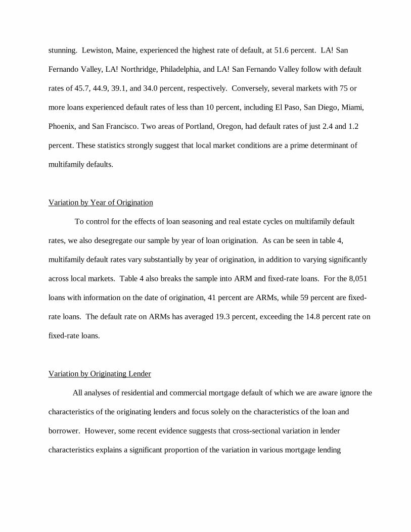
stunning. Lewiston, Maine, experienced the highest rate of default, at 51.6 percent. LA!San

Fernando Valley, LA!Northridge, Philadelphia, and LA!San Fernando Valley follow with default

rates of 45.7, 44.9, 39.1, and 34.0 percent, respectively. Conversely, several markets with 75 or

more loans experienced default rates of less than 10 percent, including El Paso, San Diego, Miami,

Phoenix, and San Francisco. Two areas of Portland, Oregon, had default rates of just 2.4 and 1.2

percent. These statistics strongly suggest that local market conditions are a prime determinant of

multifamily defaults.

Variation by Year of Origination

To control for the effects of loan seasoning and real estate cycles on multifamily default

rates, we also desegregate our sample by year of loan origination. As can be seen in table 4,

multifamily default rates vary substantially by year of origination, in addition to varying significantly

across local markets. Table 4 also breaks the sample into ARM and fixed-rate loans. For the 8,051

loans with information on the date of origination, 41 percent are ARMs, while 59 percent are fixed-

rate loans. The default rate on ARMs has averaged 19.3 percent, exceeding the 14.8 percent rate on

fixed-rate loans.

Variation by Originating Lender

All analyses of residential and commercial mortgage default of which we are aware ignore the

characteristics of the originating lenders and focus solely on the characteristics of the loan and

borrower. However, some recent evidence suggests that cross-sectional variation in lender

characteristics explains a significant proportion of the variation in various mortgage lending

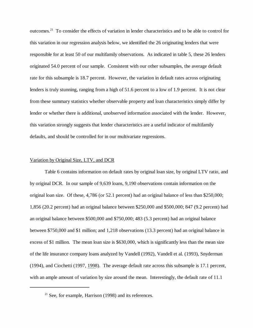
21 See, for example, Harrison (1998) and its references.

outcomes.21 To consider the effects of variation in lender characteristics and to be able to control for

this variation in our regression analysis below, we identified the 26 originating lenders that were

responsible for at least 50 of our multifamily observations. As indicated in table 5, these 26 lenders

originated 54.0 percent of our sample. Consistent with our other subsamples, the average default

rate for this subsample is 18.7 percent. However, the variation in default rates across originating

lenders is truly stunning, ranging from a high of 51.6 percent to a low of 1.9 percent. It is not clear

from these summary statistics whether observable property and loan characteristics simply differ by

lender or whether there is additional, unobserved information associated with the lender. However,

this variation strongly suggests that lender characteristics are a useful indicator of multifamily

defaults, and should be controlled for in our multivariate regressions.

Variation by Original Size, LTV, and DCR

Table 6 contains information on default rates by original loan size, by original LTV ratio, and

by original DCR. In our sample of 9,639 loans, 9,190 observations contain information on the

original loan size. Of these, 4,786 (or 52.1 percent) had an original balance of less than $250,000;

1,856 (20.2 percent) had an original balance between $250,000 and $500,000; 847 (9.2 percent) had

an original balance between $500,000 and $750,000; 483 (5.3 percent) had an original balance

between $750,000 and $1 million; and 1,218 observations (13.3 percent) had an original balance in

excess of $1 million. The mean loan size is $630,000, which is significantly less than the mean size

of the life insurance company loans analyzed by Vandell (1992), Vandell et al. (1993), Snyderman

(1994), and Ciochetti (1997, 1998). The average default rate across this subsample is 17.1 percent,

with an ample amount of variation by size around the mean. Interestingly, the default rate of 11.1

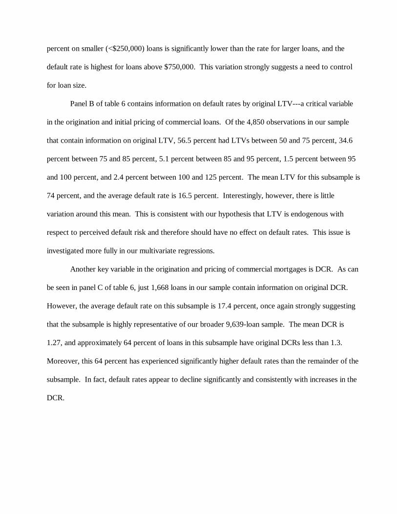
percent on smaller (<$250,000) loans is significantly lower than the rate for larger loans, and the

default rate is highest for loans above $750,000. This variation strongly suggests a need to control

for loan size.

Panel B of table 6 contains information on default rates by original LTV---a critical variable

in the origination and initial pricing of commercial loans. Of the 4,850 observations in our sample

that contain information on original LTV, 56.5 percent had LTVs between 50 and 75 percent, 34.6

percent between 75 and 85 percent, 5.1 percent between 85 and 95 percent, 1.5 percent between 95

and 100 percent, and 2.4 percent between 100 and 125 percent. The mean LTV for this subsample is

74 percent, and the average default rate is 16.5 percent. Interestingly, however, there is little

variation around this mean. This is consistent with our hypothesis that LTV is endogenous with

respect to perceived default risk and therefore should have no effect on default rates. This issue is

investigated more fully in our multivariate regressions.

Another key variable in the origination and pricing of commercial mortgages is DCR. As can

be seen in panel C of table 6, just 1,668 loans in our sample contain information on original DCR.

However, the average default rate on this subsample is 17.4 percent, once again strongly suggesting

that the subsample is highly representative of our broader 9,639-loan sample. The mean DCR is

1.27, and approximately 64 percent of loans in this subsample have original DCRs less than 1.3.

Moreover, this 64 percent has experienced significantly higher default rates than the remainder of the

subsample. In fact, default rates appear to decline significantly and consistently with increases in the

DCR.

22 Data are for 20 large life insurance companies as reported by the American Council ofLife Insurance (ACLI) Investment Bulletin series. The data are reported to represent two-thirdsof all life insurance company loan commitments.

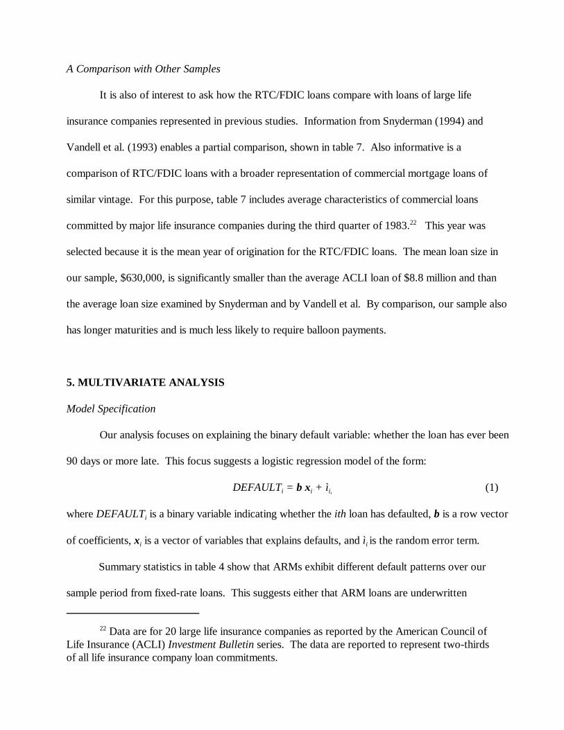
A Comparison with Other Samples

It is also of interest to ask how the RTC/FDIC loans compare with loans of large life

insurance companies represented in previous studies. Information from Snyderman (1994) and

Vandell et al. (1993) enables a partial comparison, shown in table 7. Also informative is a

comparison of RTC/FDIC loans with a broader representation of commercial mortgage loans of

similar vintage. For this purpose, table 7 includes average characteristics of commercial loans

committed by major life insurance companies during the third quarter of 1983.22 This year was

selected because it is the mean year of origination for the RTC/FDIC loans. The mean loan size in

our sample, $630,000, is significantly smaller than the average ACLI loan of $8.8 million and than

the average loan size examined by Snyderman and by Vandell et al. By comparison, our sample also

has longer maturities and is much less likely to require balloon payments.

5. MULTIVARIATE ANALYSIS

Model Specification

Our analysis focuses on explaining the binary default variable: whether the loan has ever been

90 days or more late. This focus suggests a logistic regression model of the form:

DEFAULTi = b xi + ìi, (1)

where DEFAULTi is a binary variable indicating whether the ith loan has defaulted, b is a row vector

of coefficients, xi is a vector of variables that explains defaults, and ìi is the random error term.

Summary statistics in table 4 show that ARMs exhibit different default patterns over our

sample period from fixed-rate loans. This suggests either that ARM loans are underwritten

23 Only mortgage loan observations exhibiting an original contract interest rate in excess ofthe corresponding ten-year constant maturity risk-free rate, an original LTV less than or equal to100 percent, an original DCR greater than or equal to 0.9 and less than 5.0, and an originalcontract interest rate greater than 5 percent and less than 20 percent were included in ourregression sample.

24 See Green (1977), 431.

differently from fixed-rate loans or that the underlying properties may differ between the two types

of loans, causing the “right-hand-side” variables to have relationships that differ between the two

cases. We therefore estimate separate logistic regressions for ARMs and fixed-rate mortgages.

Cleaning procedures are used to ensure that only reliable data enter our regression specifications.23

To mitigate the effect of missing values among explanatory variables, we use a technique

known as modified zero-order regression. Right-hand-side missing values for the five variables of

primary interest are set to zero. Then a companion dummy variable is created for each of the five

dummy variables, which are assigned the value of one for cases with missing data, and zero

otherwise. The regression coefficient of the dummy takes on the average incremental value

associated with the “missing value” cases, while the main coefficient of the variable represents the

marginal effect of the main variable within the set of nonmissing cases. The benefit of the technique

for this application is that it permits a very large number of cases to be used that otherwise would

have to be discarded.24 Our final fixed-rate logistic regression uses 2,966 observations; our ARM

regression sample uses 4,019. Variable definitions are provided below.

Loan and Underwriting Variables

Notwithstanding the discussion in Section 3 about the complexity of the spread variable, in

the regressions that follow a naive measure of the interest-rate risk premium is used as a predictor of

default (SPREAD). The premium is measured as the simple difference between the reported interest

rate at origination and the contemporaneous value of the ten-year constant maturity Treasury rate

(without consideration of points or mortgage insurance as substitutes for the risk premium).

SPREAD is expected to vary positively with default probability.

In addition to SPREAD, the ten-year Treasury yield (TREASYLD) also is used as a proxy

for default risk. As noted in Section 2, a higher level of interest rates at origination implies greater

subsequent decline and a greater increase in the value of the outstanding obligation, with greater

resultant reduction of borrower equity. Another argument for the variable is that mortgage rates on

loans made in a high Treasury-rate environment will be higher, and higher contract rates should be

associated with an increased probability of default, all other things being equal. Consistent with the

effect of interest-rate change on loan obligation value, the value of the borrower’s refinancing option

at any time is also higher, all other things being equal, the higher the original contract rate of interest.

Models of strategic default predict that default incidence is positively related to the incentive to

refinance. Thus, option-based models of mortgage termination predict that default rates will vary

positively with the level of interest rates at origination.

If original LTVs and DCRs are not perfect controls for loan risk, they may still correlate with

default, even after the best loan underwriting. Therefore, these ratios are also included in our

empirical analysis. Default is expected to vary positively with LTV, though if the lender over-adjusts

the ratio in underwriting, it is possible that the reverse could be true. Default is expected to vary

negatively with DCR, though again an over-adjustment of the ratio in underwriting could result in

the opposite.

All of the loans in the performance data set were/are in securitized pools. To control for

unobserved differences in pool (deal) structures, such as the presence and effectiveness of special

servicers, we include deal dummies in the logistic estimations.

Finally, all of the loans in our study were originated by financial institutions that were

eventually closed. It is likely that much variation existed in the lending and underwriting strategies of

these firms. However, by not including lender characteristics, we would effectively be assuming that

lenders are homogeneous with respect to their risk tolerances and preferences as well as their

information-gathering and processing capabilities. Therefore, controls are also constructed whereby

each financial institution represented by 50 or more loans is distinguished by a unique control

variable (INSTj). Twenty-six financial institutions are explicitly represented, with all other lenders

representing the default case. These binary variables have no expected sign. Rather, they are

intended to control for variation by lender in underwriting practices, and to test for the importance of

this variation.

Size and Property Variables

Characteristics of the collateral property may affect the likelihood of default even after

underwriting adjustments are made in the loan terms. Prominent characteristics that may be factors

are size, quality, age, and whether the property is new. It is argued in some lending circles that

larger properties are more prone to default. To account for this possibility, the number of apartment

units is included in the estimating equations to represent size (NUMUNITS), which would be

expected to have a positive sign. It has also been argued that default varies with quality. Some

have suggested that middle-quality apartments are the safest because during slumps they gain tenants

moving down and in a strong economy they gain tenants moving up. Others have argued that luxury

apartments are more risky than any others. As a measure of apartment quality, we use market value

25 As the base case, the years 1980!1982 are omitted.

per square foot at the time of loan origination (VALUE/SF). With mixed arguments as to the quality

effect, the expected sign is ambiguous.

The final property characteristic examined is age. It has been suggested by some that very

new properties present greater risk because of uncertain market acceptance, and that older properties

are risky because of cost uncertainty. Two variables are used to account for property age. A shift

variable is used to represent properties that are less than one year old at origination (NEWPROP).

In addition, the year the property was built is used to account for property age and vintage

(YRBUILT).

Seasoning and Location Variables

Both real estate markets and the interest-rate environment have shown extreme variation over

the years the loans in the study were originated, and this variation has affected default behavior in

complex ways. Rather than attempting to specify the relationship of market conditions to default,

the strategy here is to use annual shift or seasoning variables that identify either the time period

(YR71!75, YR76!79, YR83!86) or the year (YR87, . . . ,YR95) of loan origination.25 Distant

origination years are generally expected to have lower default rates than recent years because of a

higher likelihood of price appreciation.

Similarly, property location may also relate to default by capturing effects of local economic

conditions. Although this possibility is recognized by other studies, their models tend to include

location only at the state or, more commonly, regional levels. The richness of our data enable us to

distinguish location by MSA, and even sub-MSA, using three-digit zip codes. To capture the effects

of location, we identified every three-digit zip-code area represented by at least 75 loans with a shift

26 States with judicial foreclosure include Connecticut, Delaware, Florida, Illinois, Indiana,Kansas, Kentucky, Louisiana, New Jersey, New York, North Dakota, Ohio, Pennsylvania, SouthCarolina, and Wisconsin.

variable (ZIPCODEj). Twenty-six explicit three-digit zip-code areas are thus represented, as shown

in table 3, with all other areas represented in our sample constituting the default location.

Default rates may vary by state as well as by locality because of laws governing the

foreclosure process. Evidence from home mortgage loans, as shown by Clauretie (1987), indicates

that the more costly and time-consuming judicial foreclosure required by 15 states reduces the

likelihood of foreclosure relative to the likelihood in “power of sale” states.26 Ciochetti (1997) finds

that the incidence of foreclosure on commercial loans also correlates with the type of foreclosure

process. Using data reported by Ciochetti (1997), we control for the effect of foreclosure laws using

a binary variable (JUDFORE) that equals one for “judicial” states and zero for “power of sale”

states. If the requirement of judicial foreclosure inhibits foreclosure, we expect JUDFORE to have a

positive coefficient, reflecting a tendency for mortgagors to risk default more readily if foreclosure is

more difficult to effect.

Table 8 contains a comparison of our fixed-rate and ARM regression samples with all FDIC

loans that have a performance history, as well as with all 13,551 multifamily loans. The figures in

table 8 strongly suggest that our regression samples are representative of the larger multifamily data

sets. Mean loan size, percent ARMs, and the percentage of the regression sample from various

regions are generally very comparable to the larger data sets. Table 9 contains a complete list of

variable definitions for our regression sample.

Logistic Regression Results

Table 10 contains logistic regressions with parameter estimates, p-values of the associated

Wald Chi-Square statistics (in parentheses), and a measure of goodness-of-fit. The table also

contains simulation results that are discussed in the next section. The -2 Log Likelihood statistics are

highly significant for both models, indicating that the independent variables provide explanatory

power.

Loan and Underwriting Variables

None of the LTV shift variables contributes significantly to the explanatory power of the

fixed-rate default model. As discussed earlier, this would be expected if underwriters effectively use

LTV to control the level of risk. The significance of LTV for ARMs is higher, but more difficult to

interpret. The ARM LTV coefficient with the highest significance is for LTVs between 75 and 80

percent, which is the lowest risk class of the three LTV classes shown. The coefficient for the next-

higher LTV risk class (80!90 percent) is much smaller and insignificant, while the coefficient for the

highest risk class (90!100 percent) is barely significant at the 10 percent level. The LTV zero-order

coefficient is not distinguishable from zero in either the fixed-rate or ARM estimation, indicating that

the average default rate for loans missing LTV information is no different from the average default

rate on loans with LTV data. These results serve to reiterate the implications of the univariate

results shown in table 6B, which fail to show any consistent relation between LTV and default.

The coefficients on the DCR variables display some statistical significance. The probability of

default on fixed-rate and ARM loans with original DCRs between 1.1 and 1.3 are not statistically

different from loans with original DCRs between 0.90 and 1.1 (the base or omitted range).

However, the probability of default decreases as DCR increases in a reasonably consistent fashion.

For ARMs, the default rate on loans with DCRs greater than 1.3 is significantly lower (at the 7.3

percent confidence level) than the base case. The propensity to default is even lower when the DCR

exceeds 1.4. The effect of increasing DCRs on fixed-rate default is slightly less pronounced but still

statistically significant (at the 8.3 percent level) for DCRs greater than 1.4. The average default rate

for loans missing DCR information is no different from the average default rate on loans with DCR

data. In short, these DCR effects suggest that cash flow at the time of loan origination is an

important factor in default risk that is not fully controlled for by endogenous influences.

The interest-rate-risk premium coefficient (SPREAD) for both fixed-rate and ARM loans is

positive and highly significant. This suggests that lenders are cognizant of differential loan risk and

that lenders are able to rate-sort borrowers. A different effect is suggested by the positive and highly

significant coefficient on the variable for the level of interest rates at the time of origination

(TREASYLD). This coefficient suggests that higher initial interest-rate levels, hence greater decline

in rates subsequent to origination, are associated with a higher likelihood of default. From option

theory, this suggests a pattern of “strategic” default by borrowers seeking better debt terms, as

discussed in Section 2.

Size and Property Variables

There is no evidence that the probability of default varies inversely with either of the property

age variables (YRBUILT and NEWPROP) or with property quality (VALUE/SF). However, default

risk does vary positively with project size (NUMUNITS), possibly indicating that transactions costs

of default tend to be fixed and that they are less of a factor as the amount of debt is larger. The fact

that three of our four property characteristics are not significantly related to default is consistent with

the idea that lenders recognize and adjust for property risk issues, although it may also be explained

by underwriting restriction. In any event, their value as default indicators, subsequent to loan

origination, appears to be limited.

27 These include MSA191 (Central Philadelphia), MSA606 (Central Chicago), andMSA921 (San Diego). Note that all location dummy variables are included in the estimation. However, to conserve space in table 10, we report estimated coefficients and p-values only for

Seasoning Variables

An important set of coefficients concerns the year of loan origination (YR71!75, . . ., YR95),

which controls for seasoning effects. Although difficult to interpret, these coefficients provide a test

of whether changing market conditions over time are a factor in default risk. In the case of fixed-rate

mortgages, the results show the most recent (1995) and most distant origination-year (1971!1975;

1976!1979) coefficients as negative and significant, which is consistent with a “humped” shaped

default pattern commonly found in single-family mortgages. Unfortunately, since the coefficients on

the remaining fixed-rate origination-year variables cannot be distinguished from zero (not reported),

a consistent humped-shaped pattern does not emerge.

For ARMs, the story is much different. In this case the probability of default in the distant

1976!1979 period is lower than the base case, and in the more recent 1988!1991 period it is higher

than the base case. A tell-tale “hump” around the second most recent origination year is also

apparent in the ARM coefficients, and almost all are significant. Clearly, year of origination affects

ARM default rates.

Location and Lender Control Variables

An additional set of variables is included to control for the effects of local market conditions.

Six of the 26 zip-code locality variables (ZIPCODEj) dropped out of the fixed-rate model because of

a scarcity of default events. These dropout areas are effectively included in the base case. For the

remaining 20 zip-code areas, three shift coefficients are positive and significant in the fixed-rate

estimation, showing greater default likelihood.27

those location variables that are significant at the 10 percent level or greater (that is, variableswith p-values less than 0.100).

28 These include MSA852 (NE Phoenix), MSA857 (Tuscon), MSA920 (San Diego), andMSA941 (San Francisco).

29 This conclusion is supported by the fact that omission of the location variables decreasesthe overall explanatory power of the equation, as indicated by pseudo R2, from 0.2025 to 0.1904in the fixed-rate regression and from 0.1544 to 0.1308 in the ARM estimation.

Considerably more variation in default rates across zip codes is observed in ARMs. In fact,

12 of the three-digit zip-code areas experienced default rates significantly different from the base

case. Four of the ARM zip-code coefficients are negative and have relatively small standard errors,

indicating that the default experience in these areas was significantly below the base case, even after

controlling for other loan and property characteristics.28 Conversely, eight of the ARM zip-code

coefficients are significantly positive. Particularly interesting is that five of the eight are in the

greater Los Angeles area, which experienced economic weakness in the early 1990s. These results

suggest that more-refined submetropolitan data could be productive in explaining default probability,

especially for ARMs.29

The judicial foreclosure variable is difficult to interpret. Although the variable is highly

significant for fixed-rate loans, it has the opposite sign from what was expected, that is, it is negative

rather than positive. The variable also has an anomalous sign in the ARM model, although it is not

significant.

A final set of variables is included to control for the effect of lending institutions. Of the 26

originating institutions that account for at least 75 percent of the loans in our regression data sets, all

but 10 drop out because of scarcity of defaults. Of the surviving 10, 2 institutions have significant

shift coefficients in the fixed-rate regression. Only 4 institutions are associated with significantly

30 Omission of the lender identifiers decreases the pseudo R2 from 0.2025 to 0.1913 in thefixed-rate regression and from 0.1544 to 0.1448 in the ARM estimation.

different default rates in the ARM regression (2 positive, 2 negative).30 This indicates that the

extreme variation in default rates among lenders (see table 5) is attributable largely to the

characteristics of the loans rather than the lenders.

Simulated Effects of Regression Variables on Default

The previous analysis highlights the statistical significance of each loan-level attribute in

predicting default but gives no clear indication of the economic magnitude, or sensitivity, of the

characteristic. Therefore, a sensitivity analysis is performed to gauge the importance of statistically

significant characteristics. This analysis begins by constructing a base case in which each

independent variable is set at its mean value, so that it can be multiplied by its estimated regression

coefficient to determine the simulated probability of default for a standard loan. The simulated base

case probability of default is 4.1 percent for fixed-rate loans and 17.9 percent for ARMs. The base

case probabilities are similar to the actual default rates in our regression samples (8.0 percent for

fixed rate; 22.6 percent for ARMs). To simulate the magnitude of the effects of continuous variables

on default, we independently “shock” each statistically significant continuous variable by one

standard deviation, and calculate the revised probability of default. Finally, factor sensitivities are

constructed by comparing the revised probability of default with the base case. Columns two and

four of table 10 present simulated factor sensitivities for both the fixed-rate and ARM subsamples.

For example, a one standard deviation increase in the ten-year Treasury yield increases the

probability of fixed-rate and ARM default by 1.0 and 2.5 percentage points, respectively.

To simulate the effects of original DCR and LTV on default, the base case probability of

default is set to reflect the default propensity of loans with missing DCR and/or LTV data. For

example, a loan with a debt coverage ratio of 1.4 or greater has a simulated default rate that is 2.1

percentage points lower than the average default rate of loans with no DCR data. With ARM loans,

by contrast, the same probability differential is 10.8 percentage points. Overall, the effects of

increasing LTVs and decreasing DCRs are much more significant for ARMs.

To simulate the effects of three-digit zip-code location, the base case probability of default is

set to reflect the default propensity of loans from zip codes not separately identified in our sample

(that is, those with less than 100 loans in our sample). As can be seen in column two, just four zip

codes experienced higher fixed-rate default rates than the average of our noncoded zip codes.

However, location played a much more significant role in the ARM loans. In four specific zip-code

areas the probability of default was more than 25 percentage points above the base case. In two zip-

code areas it was more than 10 percentage points below.

Increases in initial DCRs are associated with decreasing default probabilities, but the effect on

ARM default rates is much more pronounced. For example, ARMs with initial DCRs in excess of

1.4 have a simulated probability of default that is 10.8 percentage points lower than ARMs with

DCRs below 1.1 (the base case). The corresponding reduction in simulated default for fixed-rate

loans is just 2.1 percentage points. Fixed-rate loans originated in states with judicial foreclosure

have a default rate that is 2.5 percentage points lower than fixed-rate loans originated in nonjudicial

foreclosure states. The existence of this characteristic has no significant effect on ARM loan default.

The simulations confirm the importance of origination year. Fixed-rate loans originated in the

1971!1975 period have an 8.8 percentage point lower probability of default than loans originated

1980!1982 (the base case range). Fixed-rate loans originated in 1976!1979 have an 8.2 percentage

point lower default probability than 1980!1982 loans. Similarly, the default probability of ARMs

originated between 1976 and 1979 is 10.5 percentage points lower than the base case ARMs. More

31 These sensitivity regressions are available from the authors upon request.

drastic is the effect on ARMs of origination during 1989, 1990, and 1991. Origination in these years

is associated with a 13.4, 19.6, and 18.3 percentage point increase, respectively, in default

probability.

The simulations also demonstrate significant effects, both positive and negative, for five

particular lending institutions. In summary, our logistic simulations provide strong evidence that our

estimated determinants of default are economically as well as statistically significant.

6. ROBUSTNESS CHECKS

Tests for Specification Sensitivity

To examine the sensitivity of our core results to variation in the specification of the logit

models, we selectively removed various combinations of variable groups. The results of this

sensitivity analysis are extremely comforting. Although overall explanatory power is reduced when a

set of control variables is eliminated, the magnitude and significance of our core loan variables

remain virtually unchanged.31

Tests for Left-Censuring Effects

As discussed in Section 3, left censuring is difficult to avoid in default studies and can clearly

bias univariate estimates of default frequency. Thus, all of the simple marginal distributions of

default frequency reported here are likely to understate or overstate the overall frequency of default

in the original loan population, depending on whether early defaults or early payoffs were

disproportionately high. However, the effect of left censuring is less obvious for the results of

multivariate analysis. The issue in the multivariate context is whether early exits from the loan

32 To illustrate the point, consider a set of 1,000 loans, of which 100 have defaulted. Further, suppose that some characteristic of the loans exhibits a 70 percent correlation withdefault, and that half of the defaulted loans have left the sample. While the estimated default rateclearly will be biased downward (50/950), there is no implied change in the observed correlation.

population, because of payoff or default, alter the interrelationships among the variables of the

analysis for the surviving population. While early exits may have a persuasively clear effect on

frequency distributions, they do not have a clear effect on multivariate relationships.32

To test for the effect of left censuring on multivariate findings, we identified all loans in the

sample that were originated within two and three years of the time of securitization (the beginning of

our records). Note that the substance of this distinction is “new” versus “seasoned” loans. The

conventional wisdom appears to be that loans with high original LTVs and loans with low original

DCRs will tend to default at high rates, and early. Thus the “seasoned” pool will evidence less

relationship of these underwriting variables to default as the high-risk loans are censured out through

default. The “new” versus “seasoned” distinction enables us to test for this possibility. If there is a

difference in the multivariate relationships, “new” loans should evidence positive coefficients for our

LTV categories and negative coefficients for our DCR categories.

The “new” loans constitute a relatively small portion of the entire sample of 9,637 (640 were

originated within two years before securitization and 1,262 were originated within three years).

Rather than analyzing them separately, we created interactive “dummy” variables in our main

equations (both fixed rate and ARM) for each underwriting variable category, including all LTV

categories, all debt coverage categories, and the interest-rate-spread variable.

The results of our tests can be summarized succinctly. Not one underwriting variable had an

additional significant coefficient result from the “new” loans for either fixed-rate loans or ARMs.

Only one “new” loan coefficient was significant, but this was for ARMs with DCRs above 1.4, which

33 This is the ARM coefficient for DCRs between 1.3 and 1.4 on “new” loans, where newloans are defined as three years before securitization. By conventional wisdom, this coefficientshould be negative, but it is positive, and significant at the 5 percent level. The second coefficient

were already significant when “new” loans were not distinguished. The related base coefficient

ceases to be significant when “new” loans are distinguished. Meanwhile, when “new” is defined as

two years before securitization, the interest-rate-spread variable for fixed-rate loans is positive and

significant at the 4 percent level of probability. (The latter result is consistent with the hypothesis

discussed in Section 2, that lenders adjust the spread to control for residual default risk.) In

summary, these results do not support the argument that populations of seasoned loans and new

loans show different relationships between underwriting variables and default risk.

Multicolinearity among Underwriting Variables

We have argued that the three variables LTV, DCR , and interest-rate spread are likely to be

endogenously and simultaneously determined. If so, they may also be strongly correlated, and this

multicolinearity may explain the insignificant coefficients for the underwriting variables. We test this

possibility using three modified sets of regressions. In each set only one of the three variables is used

in the regression. (However, the distinction between “new” and “seasoned” loans is maintained,

using both the two-year and three-year definition.) If multicolinearity is the explanation for

insignificant coefficients, removing two of the three variables should eliminate the problem, allowing

the remaining variable to proxy for the effect of all three.

The results of our tests for multicolinearity, again, may be summarized succinctly. In every

test, removing two of the three variables reduced the explanatory power of the equation as measured

by pseudo R2. However, only two underwriting coefficients became significant that previously were

not, and one of these has the wrong sign.33 Of 64 regression coefficients that could have signaled

that becomes positive is the ARM coefficient for LTVs between 90 and 100 percent on newloans. This coefficient is positive and significant at the 9 percent level.

some evidence of multicolinearity (16 in each of four test equations), only one was significantly

changed and carried the correct sign. In short, we see little support for the hypothesis that the

general lack of significance of our underwriting coefficients is due to multicolinearity.

7. SUMMARY AND CONCLUSIONS

The large growth in commercial mortgage securities during the past decade has led to

substantial research on the valuation and pricing of these securities. However, in contrast to research

involving the residential mortgage market, the available data have severely constrained research on

the patterns and causes of commercial mortgage defaults and prepayments. Despite the strong

implications of option-based default models regarding default risk indicators, little testing of their

usefulness has occurred. Further, little is known about the influences of property values, cash flows,

and other loan, property, and lender characteristics on default.

This paper examines the default experience of multifamily mortgages that were incorporated

in RTC/FDIC CMBS brought to market between 1991 and 1996. This unique data set contains

extensive property, loan, and underwriting data, plus a recent record of loan performance. The

performance record also contains the month of default and the default resolution (modification,

foreclosure, etc.). These data support multivariate analysis of default not possible in previous

studies.

Our loan performance data set contains 9,639 multifamily mortgages. The descriptive

statistics we report display substantial variation in default rates across states, zip codes, year of

origination, originating lender, original loan size, LTV, DCR, and loan type (fixed rate versus ARM).

The dependent variable is a binary classification: whether the loan has ever been 90 days late.

Recognizing that fixed-rate and ARM default patterns are very distinct, we performed separate

regressions on each loan type.

The original LTV does not contribute significantly to the explanatory power of the fixed-rate

model, and its significance in the ARM model is difficult to interpret. In contrast, the expected

inverse relation between incidence of default and DCR seems more consistent, although this effect is

again stronger in the ARM specification. The spread between the contract interest rate and the ten-

year Treasury yield at origination is positive and highly significant, which is consistent with the

notion that lenders recognize differential loan risk and are able to rate-sort borrowers. Moreover,

the coefficient on the interest-rate level at the time of origination is positive and highly significant,

suggesting that higher initial interest rates increase the likelihood of default, all other things being

equal. Somewhat surprisingly, the level of interest rates affects both ARM and fixed-rate defaults,

thereby limiting the ability to interpret the effect in a traditional option framework. More generally,

the results suggest that endogenous elements appear to interact with option-related factors to

produce considerable complexity in the determinants of multifamily default.

Three of our four property characteristics---year built, a proxy for quality, and an indicator of

a newly constructed property---are not significant. A number of our shift variables that capture (and

control for) the effects of origination year are statistically significant, especially in the ARM

regression. In addition, the inclusion of location control variables (three-digit zip codes) contributed

significantly to the explanatory power of the models, suggesting that even more refined

submetropolitan data could be productive in explaining default probability. Finally, the extreme

variation in default rates among lenders appears to be largely, but not entirely, attributable to the

characteristics of the loans rather than the lenders.

The degree to which the findings can be generalized is, of course, not fully clear, and further

investigation is needed. For example, although the mortgages studied in this paper came from many

institutions and geographic areas, they also came from institutions that were, or became, insolvent.

Although the loans were performing before being placed into the RTC/FDIC CMBS, we do not

know whether or how their derivation from insolvent institutions affects the results. However, this

concern is considerably assuaged by the fact that the cumulative default rate of the sample is 17.5

percent, which does not differ significantly from the apparent default frequency experience of loans

held by major life insurance companies. This fact is especially notable, given that our definition of

default is considerably broader than that employed by previous studies.

To the extent that our findings are valid, they generally confirm (for fixed-rate loans, though

less for ARMs) that underwriting variables, especially LTV, are endogenously affected by the loan

origination process and that this renders them poor indicators of subsequent default. On the other

hand, the spread between loan and market interest rates, which logically should reflect default risk in

an endogenous risk framework, shows empirical evidence of doing so.

References

Archer, Wayne R., David C. Ling, and Gary McGill. 1996. The Effect of Income and CollateralConstraints on Residential Mortgage Terminations. Regional Science and Urban Economics26:235!261.

Bradley, Donald S., Frank E. Nothaft, and James L. Freund. 1998. Financing MultifamilyProperties: A Play with New Actors and New Lines. Cityscape: A Journal of Housing andUrban Development 4:5!17.

Capozza, Dennis R., Dick Kazarian, and Thomas Thomson. 1998. The Conditional Probability ofMortgage Default. Real Estate Economics 26:359!390.

Childs, Paul D., Steven H. Ott, and Timothy Riddiough. 1996. The Value of Recourse and Cross-Default Clauses in Commercial Mortgage Contracting. Journal of Banking and Finance20:511!536.

Ciochetti, Brian A. 1997. Loss Characteristics of Commercial Mortgage Foreclosures. Real EstateFinance 14:53!69.

))))) . 1998. Investment Loss Characteristics Associated with Commercial Mortgage Foreclosures. Working Paper, University of North Carolina.

Ciochetti, Brian A., and Timothy J. Riddiough. 1998. Timing, Loss Recovery and EconomicPerformance of Foreclosed Commercial Mortgages. Working Paper, University of NorthCarolina and M.I.T.

Ciochetti, Brian A., and Kerry D. Vandell. 1999. The Performance of Commercial Mortgages. Real Estate Economics 27:27!61.

Clauretie, Terrence M. 1987. The Impact of Interstate Foreclosure Cost Differences and the Valueof Mortgages on Default Rates. AREUEA Journal 15:152!167.

Cox, John C., and Mark Rubinstein. 1985. Options Markets. Prentice Hall.

Cunningham, Donald, and Patric H. Hendershott. 1995. Pricing FHA Mortgage Default Insurance. Housing Finance Review 13:373!392.

Deng, Yongheng. 1997. Mortgage Termination: An Empirical Hazard Model with a StochasticTerm Structure. The Journal of Real Estate Finance and Economics 14:309!332.

Elmer, Peter J., and Anton E. Haidorfer. 1997. Prepayments of Multifamily Mortgage-BackedSecurities. Journal of Fixed Income 6:50!63.

Elmer, Peter J., and Steven A. Seelig. 1999. Insolvency, Trigger Events, and Consumer RiskPosture in the Theory of Single-Family Mortgage Default. Journal of Housing Research(forthcoming).

Episcopos, Athanasios, Andreas Pericli, and Jianxun Hu. 1998. Commercial Mortgage Default: AComparison of Logit with Radial Basis Function Networks. The Journal of Real EstateFinance and Economics, 17:163!178.

Fitch. 1996. Trends in Commercial Mortgage Default Rates and Loss Severity. Fitch InvestorsService, LP, Special Report, November 11.

Follain, James R., Wenyi-Vivien Huang, and Jan Ondrich. 1999. Stay, Pay or Walk Away: AHazard Analysis of FHA-Insured Multifamily Mortgage Terminations. Draft paper.

Foster, Charles, and Robert Van Order. 1985. FHA Terminations: A Prelude to Rational MortgagePricing. Journal of the American Real Estate and Urban Economics Association13:292!316.

Gau, George W., and Ko Wang. 1994. The Tax-Induced Holding Periods of Real Estate Investors:Theory and Empirical Evidence. The Journal of Real Estate Finance and Economics 8:71!85.

Goldberg, Lawrence, and Charles A. Capone, Jr. 1998. Multifamily Mortgage Credit Risk: Lessonsfrom Recent History. Cityscape: A Journal of Housing and Urban Development 4:93!113.

Green, William H. 1997. Econometric Analysis, 5th ed. Prentice Hall.

Harrison, David M. 1998. The Importance of Lender Heterogeneity in Mortgage Lending. Working Paper, University of Vermont.

Hilliard, Jimmy E., James B. Kau, and Carlos Slawson, Jr. 1998. Valuing Prepayment and Default

in a Fixed-Rate Mortgage: A Bivariate Binomial Options Pricing Technique. Real EstateEconomics 26:431!468.

Kau, James B., Donald C. Keenan, Walter J. Muller, and James F. Epperson. 1987. The Valuationof Commercial and Multifamily Mortgages. Journal of Banking and Finance 11: 525!546.

))))) . 1990. Pricing Commercial Mortgages and Their Mortgage-Backed Securities. The Journalof Real Estate Finance and Economics 3:333!336.

Nelson, Grant S., and Dale A. Whitman. 1993. Real Estate Finance Law. 3d ed. West PublishingCo.

Quigg, Laura. 1997. Analyzing CMBS Performance–A Discussion of the Fitch Study. J.P. MorganSecurities Inc. Credit Research, January 6.

))))) . 1998. Default Risk in CMBS Bond Classes. In Trends in Commercial Mortgage-Backed Securities, edited by Frank J. Fabozzi Associates.

Riddiough, Timothy J., and Steve B. Wyatt. 1994. Strategic Default, Workout, and CommercialMortgage Valuation. Journal of Real Estate Finance and Economics 9:5!22.

Snyderman, Mark P. 1994. Update on Commercial Mortgage Defaults. The Real Estate FinanceJournal (summer) 22!32.

Vandell, Kerry D. 1995. How Ruthless Is Mortgage Default? A Review and Synthesis of theEvidence. Journal of Housing Research 6:245!264.

))))) . 1992. Predicting Commercial Mortgage Foreclosure. Real Estate Economics 20:55!88.

Vandell, Kerry D., Walter Barnes, David Hartzell, Dennis Kraft, and William Wendt. 1993.Commercial Mortgage Defaults: Proportional Hazards Estimation Using Individual LoanHistories. Journal of the American Real Estate and Urban Economics Association21:451!480.

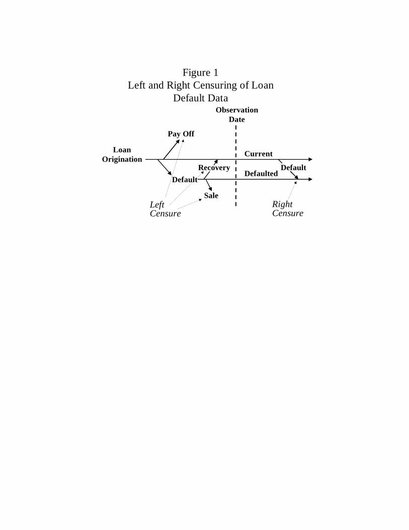
Figure 1Left and Right Censuring of Loan

Default Data

LoanOrigination

Pay Off

Default

Sale

ObservationDate

Defaulted

Current

Recovery Default

LeftCensure

RightCensure

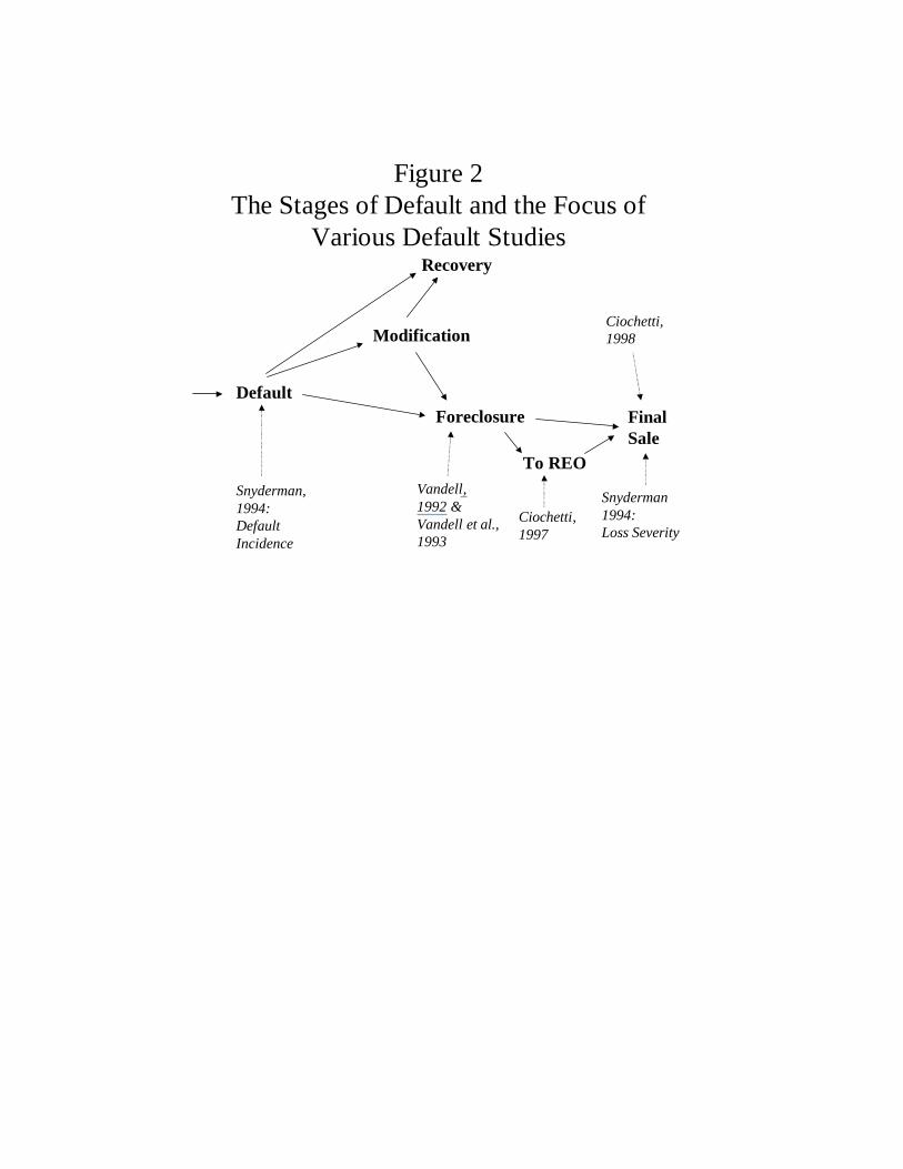
Default

Modification

Recovery

Foreclosure

To REO

FinalSale

Figure 2The Stages of Default and the Focus of

Various Default Studies

Snyderman, 1994:DefaultIncidence

Snyderman1994:Loss Severity

Vandell, 1992 & Vandell et al.,1993

Ciochetti,1997

Ciochetti,1998

Table 1Tabulation of Default Rates by Deal

Deal

# ofLendersin Deal

# of MultiLoans

Originally inDeal

Total # ofMulti

Loans inSample

% of OriginalMulti Loansin Sample

SampleLoans in

Deal as % ofTotal Sample

SampleDefault

Rate (%)

Multifamily Deals

1991-M11991-M21991-M31991-M41991-M51991-M61991-M71991-M11991-M21991-M31991-M4

2 1 5 5 3 321 2528975

218 517 137

1,388 548 391 591 787

1,410 1,410 988

185406100917275281334582962895685

84.978.573.066.150.271.956.574.068.263.569.3

1.94.21.09.52.92.93.56.0

10.0 9.37.1

41.648.528.015.710.221.714.413.413.312.019.9

8,385 5,622 67.0% 58.3% 18.4%

Commercial Deals*

1992-C41992-C51992-C61992-C71993-C21993-C31994-C11994-C21995-C11995-C21996-C1F

68169136 78272237238234222111183

303538633368662287941453629263285

174280 54237556225875437606283290

57.452.0 8.564.484.078.493.096.596.3

107.6 101.8

1.82.90.62.55.82.39.14.56.32.93.0

15.512.568.521.121.415.116.822.7 8.311.7 6.9

5,362 4,017 74.9% 41.7% 16.2%

Total Multi Loans in Multi and Com Deals

13,747 9,639 70.1% 100.0% 17.5%

*The number of multifamily loans in commercial deals is estimated from the prospectus. Thus, this number mayvary slightly from the actual number of loans in the transaction at closing.

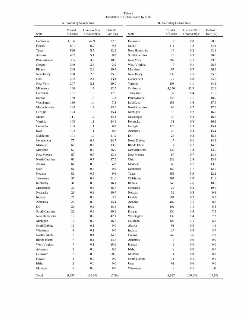
Table 2Tabulation of Default Rates by State

A. Sorted by Sample Size B. Sorted by Default Rate

StateTotal #of Loans

Loans as % of Total Sample

DefaultRate (%) State

Total #of Loans

Loans as % ofTotal Sample

DefaultRate (%)

CaliforniaFloridaTexasArizonaPennsylvaniaOregonIllinoisNew JerseyOhioNew YorkMinnesotaLouisianaKansasWashingtonMassachusettsGeorgiaMaineVirginiaColoradoIowaOklahomaConnecticutMissouriMarylandNew MexicoNorth CarolinaAlaskaUtahNevadaTennesseeKentuckyMississippiNebraskaIndianaArkansasDCSouth CarolinaNew HampshireMichiganSouth DakotaWisconsinNorth DakotaRhode IslandWest VirginiaArkansasDelawareHawaiiIdahoMontana

4,136 601566487355349249238232207160151150139133123111108103102101 77 69 67 67 63 61 61 52 37 31 30 28 27 26 26 26 19 18 11 9 7 7 7 3 2 2 2 1

42.9 6.25.95.13.73.62.62.52.42.11.71.61.61.41.41.31.21.11.11.11.00.80.70.70.70.70.60.60.50.40.30.30.30.30.30.30.30.20.20.10.10.10.10.10.00.00.00.00.0

22.3 9.312.2 8.818.9 2.910.825.613.429.012.517.9 7.3 7.213.515.444.124.1 6.8 8.811.924.713.026.913.417.5 4.9 0.0 9.621.616.116.710.7 3.715.415.430.842.116.7 0.0 0.014.314.328.6 0.050.0 0.0 0.0 0.0

DelawareMaineNew HampshireSouth CarolinaNew YorkWest VirginiaMarylandNew JerseyConnecticutVirginiaCaliforniaTennesseePennsylvaniaLouisianaNorth CarolinaMichiganMississippiKentuckyGeorgiaArkansasDCNorth DakotaRhode IslandMassachusettsNew MexicoOhioMissouriMinnesotaTexasOklahomaIllinoisNebraskaNevadaFloridaArizonaIowaKansasWashingtonColoradoAlaskaIndianaOregonArkansasHawaiiIdahoMontanaSouth DakotaUtahWisconsin

2111 19 26207 7 67238 77108

4,136 37355151 63 18 30 31123 26 26 7 7133 67232 69160566101249 28 52601487102150139103 61 27349 3 2 2 1 11 61 9

0.01.20.20.32.10.10.72.50.81.1

42.9 0.43.71.60.70.20.30.31.30.30.30.10.11.40.72.40.71.75.91.02.60.30.56.25.11.11.61.41.10.60.33.60.00.00.00.00.10.60.1

50.044.142.130.829.028.626.925.624.724.122.321.618.917.917.516.716.716.115.415.415.414.314.313.513.413.413.012.512.211.910.810.7 9.6 9.3 8.8 8.8 7.3 7.2 6.8 4.9 3.7 2.9 0.0 0.0 0.0 0.0 0.0 0.0 0.0

Total 9,637 100.0% 17.5% 9,637 100.0% 17.5%

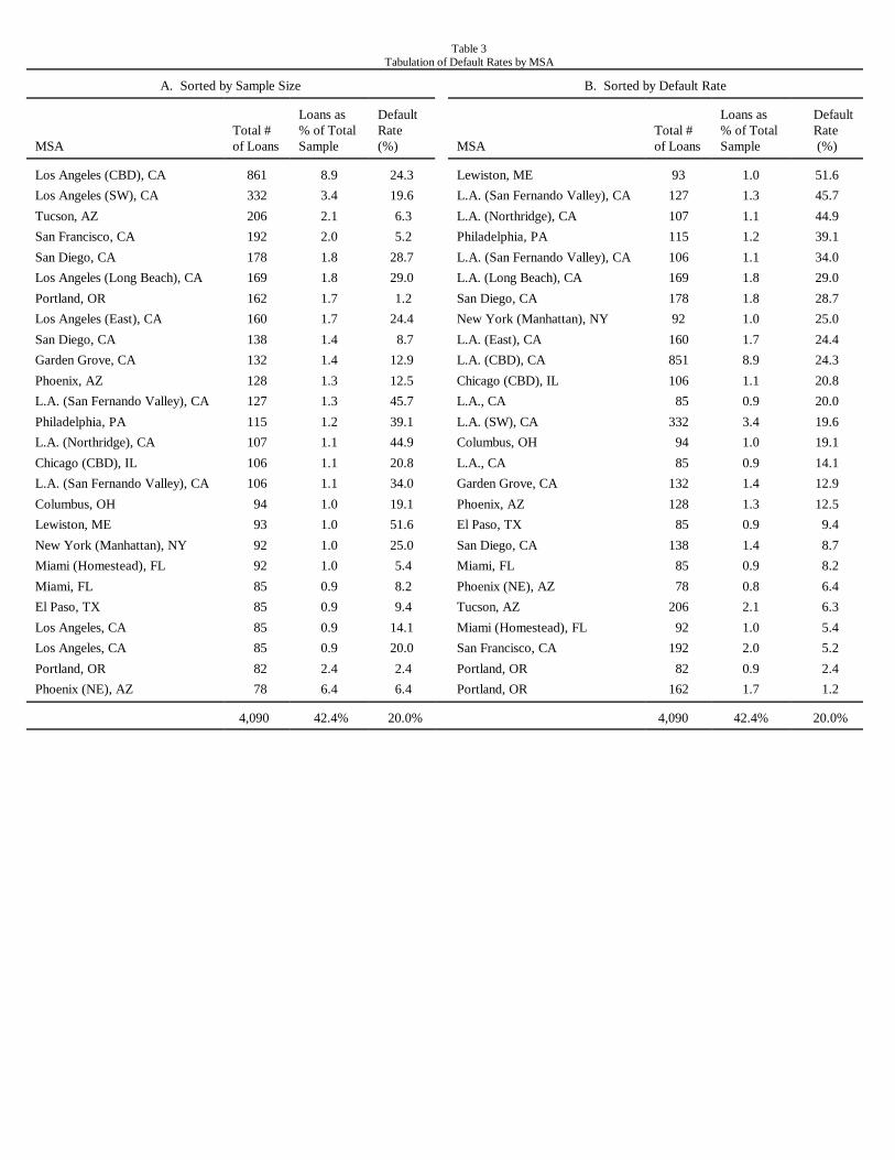
Table 3Tabulation of Default Rates by MSA

A. Sorted by Sample Size B. Sorted by Default Rate

MSATotal # of Loans

Loans as % of TotalSample

DefaultRate(%) MSA

Total # of Loans

Loans as % of TotalSample

Default Rate (%)

Los Angeles (CBD), CALos Angeles (SW), CATucson, AZSan Francisco, CASan Diego, CALos Angeles (Long Beach), CAPortland, ORLos Angeles (East), CASan Diego, CAGarden Grove, CAPhoenix, AZL.A. (San Fernando Valley), CAPhiladelphia, PAL.A. (Northridge), CAChicago (CBD), ILL.A. (San Fernando Valley), CAColumbus, OHLewiston, MENew York (Manhattan), NYMiami (Homestead), FLMiami, FLEl Paso, TXLos Angeles, CALos Angeles, CAPortland, ORPhoenix (NE), AZ

861332206192178169162160138132128127115107106106 94 93 92 92 85 85 85 85 82 78

8.93.42.12.01.81.81.71.71.41.41.31.31.21.11.11.11.01.01.01.00.90.90.90.92.46.4

24.319.6 6.3 5.228.729.0 1.224.4 8.712.912.545.739.144.920.834.019.151.625.0 5.4 8.2 9.414.120.0 2.4 6.4

Lewiston, MEL.A. (San Fernando Valley), CAL.A. (Northridge), CAPhiladelphia, PAL.A. (San Fernando Valley), CAL.A. (Long Beach), CASan Diego, CANew York (Manhattan), NYL.A. (East), CAL.A. (CBD), CAChicago (CBD), ILL.A., CAL.A. (SW), CAColumbus, OHL.A., CAGarden Grove, CAPhoenix, AZEl Paso, TXSan Diego, CAMiami, FLPhoenix (NE), AZTucson, AZMiami (Homestead), FLSan Francisco, CAPortland, ORPortland, OR

9312710711510616917892160851106 85332 94 85132128 85138 85 78206 92192 82162

1.01.31.11.21.11.81.81.01.78.91.10.93.41.00.91.41.30.91.40.90.82.11.02.00.91.7

51.645.744.939.134.029.028.725.024.424.320.820.019.619.114.112.912.5 9.4 8.7 8.2 6.4 6.3 5.4 5.2 2.4 1.2

4,090 42.4% 20.0% 4,090 42.4% 20.0%

Table 4Tabulation of Default Rates by Origination Year

All Loans ARM Loans Fixed-Rate Loans

Year ofOrigination

Total # ofLoans

Loans as %of Sample

DefaultRate

Total # ofARM Loans

Loans as % ofTotal Sample

DefaultRate (%)

Total # ofLoans

Loans as % ofTotal Sample

DefaultRate (%)

70717273747576777879808182838485868788899091929394959697

34149340264128242384463322138 68 41 49233272373618764

1,077 817327174138158353121 3 1

0.41.94.23.31.63.04.85.84.01.70.80.50.62.93.44.67.79.5

13.4 10.1 4.12.21.72.04.41.50.00.0

14.7 4.7 2.9 1.9 6.3 3.7 3.9 3.7 5.9 7.217.612.224.510.716.518.517.321.528.233.931.523.613.012.7 7.4 5.8 0.0 0.0

2 5 4 2 42081976110232029

178 211 258 365 473 723 346 151 89544056 9 1 1

0.00.10.00.00.00.21.01.20.80.10.30.20.42.22.63.24.55.99.04.31.91.10.70.50.70.10.00.0

0.00.0

25.0 0.0

50.0 0.02.55.23.3

20.0 17.4 5.0

20.7 9.6

11.4 14.7 14.0 18.4 27.2 27.2 35.1 30.3 20.4 20.0 14.3 0.00.00.0

321443362621242223033662611284521205561115253291354471176858411829711220

0.41.84.23.31.52.83.84.53.21.60.60.30.20.70.81.43.13.64.45.92.21.11.01.53.71.40.00.0

15.64.92.71.94.84.14.33.36.56.317.819.030.014.534.427.022.126.530.238.928.416.58.310.26.16.30.0

8,051 100.0% 16.6% 3,313 41.2% 19.3% 4,738 58.8% 14.8%

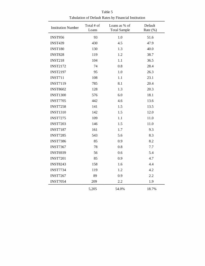
Table 5Tabulation of Default Rates by Financial Institution

Institution Number Total # of Loans

Loans as % of Total Sample

Default Rate (%)

INST956INST439INST180INST828INST218INST2172INST2197INST711INST7119INST8602INST1300INST7705INST7258INST1310INST7275INST7203INST7187INST7285INST7386INST7367INST6939INST7201INST8243INST7734INST7267INST7054

93 430 130 119 104 74 95 108 785 128 576 442 141 142 109 146 161 543 85 78 56 85 158 119 89 209

1.04.51.31.21.10.81.01.18.11.36.04.61.51.51.11.51.75.60.90.80.60.91.61.20.92.2

51.647.940.038.736.528.426.323.120.420.318.113.613.512.011.011.0 9.3 8.3 8.2 7.7 5.4 4.7 4.4 4.2 2.2 1.9

5,205 54.0% 18.7%

Table 6Default Rates by Original Loan Size, Original

Loan-to-Value (LTV) Ratio, and Original DCR

A. By Original Loan Size

Original Loan Size

($000)Total #

of Loans

Loans as % ofSample

DefaultRate (%)

Below $250$250<$500$500<$750

$750<$1,000Over $1,000

4,786 1,856 847 4831,218

52.120.2 9.2 5.313.3

11.120.522.429.427.1

9,190 100.0% 17.1%

B. By Original LTV

Original Loan Size

($000)Total #

of Loans

Loans as % of Sample

DefaultRate (%)

50%<75%75%<85%85%<95%

95%<100%100%<125%

2,7381,677 246 75 114

56.534.6 5.1 1.5 2.4

15.218.816.314.714.9

4,850 100.0% 16.5%

C. By Original Debt Coverage Rate

DCR Total #of Loans

Loans as % of Sample

DefaultRate (%)

Below 1.01.0<1.11.1<1.21.2<1.31.3<1.41.4<1.51.5<1.61.6<1.71.7<1.81.8<1.91.9<2.02.0<3.0

390 224 244 206 140 100 64 62 42 50 23 123

23.413.414.612.4 8.4 6.0 3.8 3.7 2.5 3.0 1.4 7.4

23.122.826.618.410.010.0 7.8 4.8 2.4 8.0 8.7 5.7

1,668 100.0% 17.4%

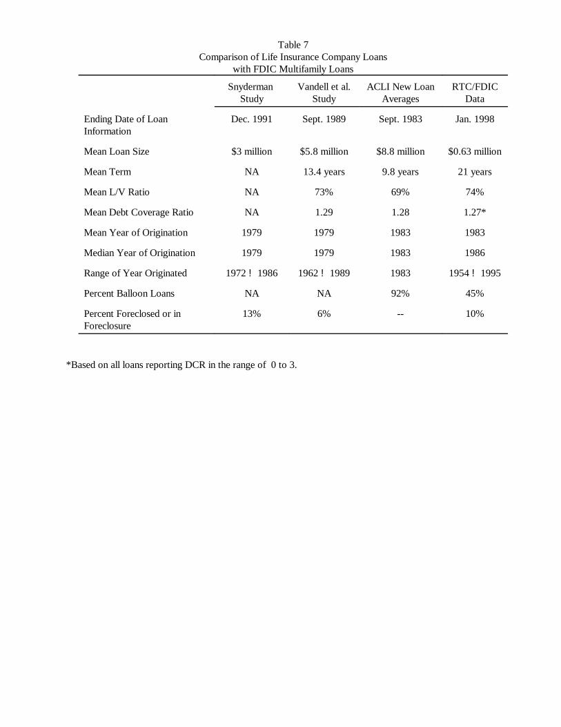
Table 7Comparison of Life Insurance Company Loans

with FDIC Multifamily Loans

Snyderman Study

Vandell et al.Study

ACLI New LoanAverages

RTC/FDICData

Ending Date of LoanInformation

Dec. 1991 Sept. 1989 Sept. 1983 Jan. 1998

Mean Loan Size $3 million $5.8 million $8.8 million $0.63 million

Mean Term NA 13.4 years 9.8 years 21 years

Mean L/V Ratio NA 73% 69% 74%

Mean Debt Coverage Ratio NA 1.29 1.28 1.27*

Mean Year of Origination 1979 1979 1983 1983

Median Year of Origination 1979 1979 1983 1986

Range of Year Originated 1972 ! 1986 1962 ! 1989 1983 1954 ! 1995

Percent Balloon Loans NA NA 92% 45%

Percent Foreclosed or inForeclosure

13% 6% -- 10%

*Based on all loans reporting DCR in the range of 0 to 3.

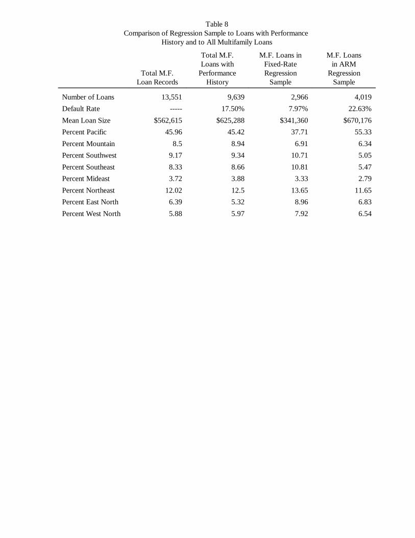
Table 8Comparison of Regression Sample to Loans with Performance

History and to All Multifamily Loans

Total M.F.Loan Records

Total M.F.Loans with

PerformanceHistory

M.F. Loans inFixed-RateRegression

Sample

M.F. Loansin ARM

RegressionSample

Number of LoansDefault RateMean Loan SizePercent PacificPercent MountainPercent SouthwestPercent SoutheastPercent MideastPercent NortheastPercent East NorthPercent West North

13,551-----

$562,61545.96

8.59.178.333.72

12.026.395.88

9,63917.50%

$625,28845.428.949.348.663.8812.55.325.97

2,9667.97%

$341,36037.716.91

10.7110.813.33

13.658.967.92

4,01922.63%

$670,17655.336.345.055.472.79

11.656.836.54

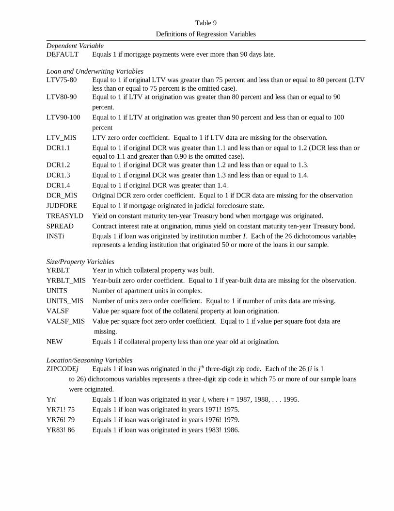
Table 9Definitions of Regression Variables

Dependent VariableDEFAULT Equals 1 if mortgage payments were ever more than 90 days late.

Loan and Underwriting VariablesLTV75-80 Equal to 1 if original LTV was greater than 75 percent and less than or equal to 80 percent (LTV

less than or equal to 75 percent is the omitted case).LTV80-90 Equal to 1 if LTV at origination was greater than 80 percent and less than or equal to 90

percent.LTV90-100 Equal to 1 if LTV at origination was greater than 90 percent and less than or equal to 100

percentLTV_MIS LTV zero order coefficient. Equal to 1 if LTV data are missing for the observation.DCR1.1 Equal to 1 if original DCR was greater than 1.1 and less than or equal to 1.2 (DCR less than or

equal to 1.1 and greater than 0.90 is the omitted case). DCR1.2 Equal to 1 if original DCR was greater than 1.2 and less than or equal to 1.3.DCR1.3 Equal to 1 if original DCR was greater than 1.3 and less than or equal to 1.4.DCR1.4 Equal to 1 if original DCR was greater than 1.4.DCR_MIS Original DCR zero order coefficient. Equal to 1 if DCR data are missing for the observationJUDFORE Equal to 1 if mortgage originated in judicial foreclosure state.TREASYLD Yield on constant maturity ten-year Treasury bond when mortgage was originated.SPREAD Contract interest rate at origination, minus yield on constant maturity ten-year Treasury bond. INSTi Equals 1 if loan was originated by institution number I. Each of the 26 dichotomous variables

represents a lending institution that originated 50 or more of the loans in our sample.

Size/Property VariablesYRBLT Year in which collateral property was built.YRBLT_MIS Year-built zero order coefficient. Equal to 1 if year-built data are missing for the observation.UNITS Number of apartment units in complex.UNITS_MIS Number of units zero order coefficient. Equal to 1 if number of units data are missing. VALSF Value per square foot of the collateral property at loan origination. VALSF_MIS Value per square foot zero order coefficient. Equal to 1 if value per square foot data are

missing.NEW Equals 1 if collateral property less than one year old at origination.

Location/Seasoning VariablesZIPCODEj Equals 1 if loan was originated in the jth three-digit zip code. Each of the 26 (i is 1

to 26) dichotomous variables represents a three-digit zip code in which 75 or more of our sample loanswere originated.

Yri Equals 1 if loan was originated in year i, where i = 1987, 1988, . . . 1995.YR71!75 Equals 1 if loan was originated in years 1971!1975.YR76!79 Equals 1 if loan was originated in years 1976!1979.YR83!86 Equals 1 if loan was originated in years 1983!1986.

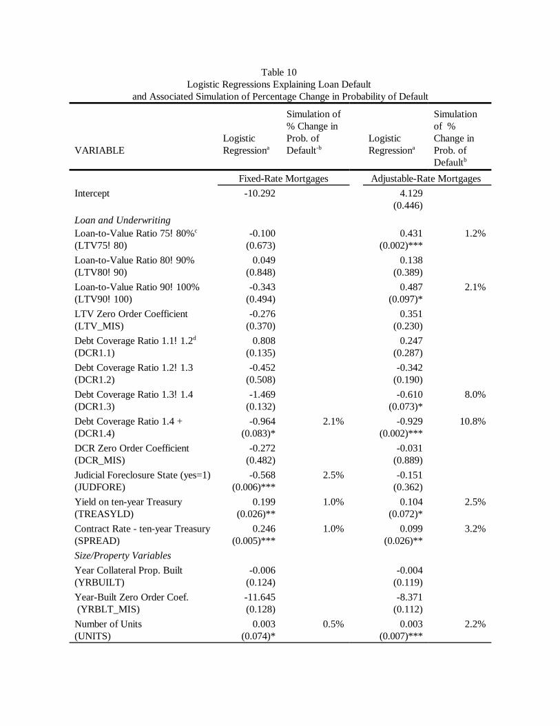
Table 10 Logistic Regressions Explaining Loan Default

and Associated Simulation of Percentage Change in Probability of Default

VARIABLELogisticRegressiona

Simulation of% Change inProb. ofDefault-b

LogisticRegressiona

Simulationof %Change inProb. ofDefaultb

Fixed-Rate Mortgages Adjustable-Rate Mortgages Intercept -10.292 4.129

(0.446)Loan and UnderwritingLoan-to-Value Ratio 75!80%c

(LTV75!80)-0.100

(0.673)0.431

(0.002)***1.2%

Loan-to-Value Ratio 80!90%(LTV80!90)

0.049(0.848)

0.138(0.389)

Loan-to-Value Ratio 90!100%(LTV90!100)

-0.343(0.494)

0.487(0.097)*

2.1%

LTV Zero Order Coefficient(LTV_MIS)

-0.276(0.370)

0.351(0.230)

Debt Coverage Ratio 1.1!1.2d

(DCR1.1)0.808

(0.135)0.247

(0.287)Debt Coverage Ratio 1.2!1.3(DCR1.2)

-0.452(0.508)

-0.342(0.190)

Debt Coverage Ratio 1.3!1.4(DCR1.3)

-1.469(0.132)

-0.610(0.073)*

8.0%

Debt Coverage Ratio 1.4 +(DCR1.4)

-0.964(0.083)*

2.1% -0.929(0.002)***

10.8%

DCR Zero Order Coefficient(DCR_MIS)

-0.272(0.482)

-0.031(0.889)

Judicial Foreclosure State (yes=1)(JUDFORE)

-0.568(0.006)***

2.5% -0.151(0.362)

Yield on ten-year Treasury(TREASYLD)

0.199(0.026)**

1.0% 0.104(0.072)*

2.5%

Contract Rate - ten-year Treasury(SPREAD)

0.246(0.005)***

1.0% 0.099(0.026)**

3.2%

Size/Property VariablesYear Collateral Prop. Built(YRBUILT)

-0.006(0.124)

-0.004(0.119)

Year-Built Zero Order Coef. (YRBLT_MIS)

-11.645(0.128)

-8.371(0.112)

Number of Units(UNITS)

0.003(0.074)*

0.5% 0.003(0.007)***

2.2%

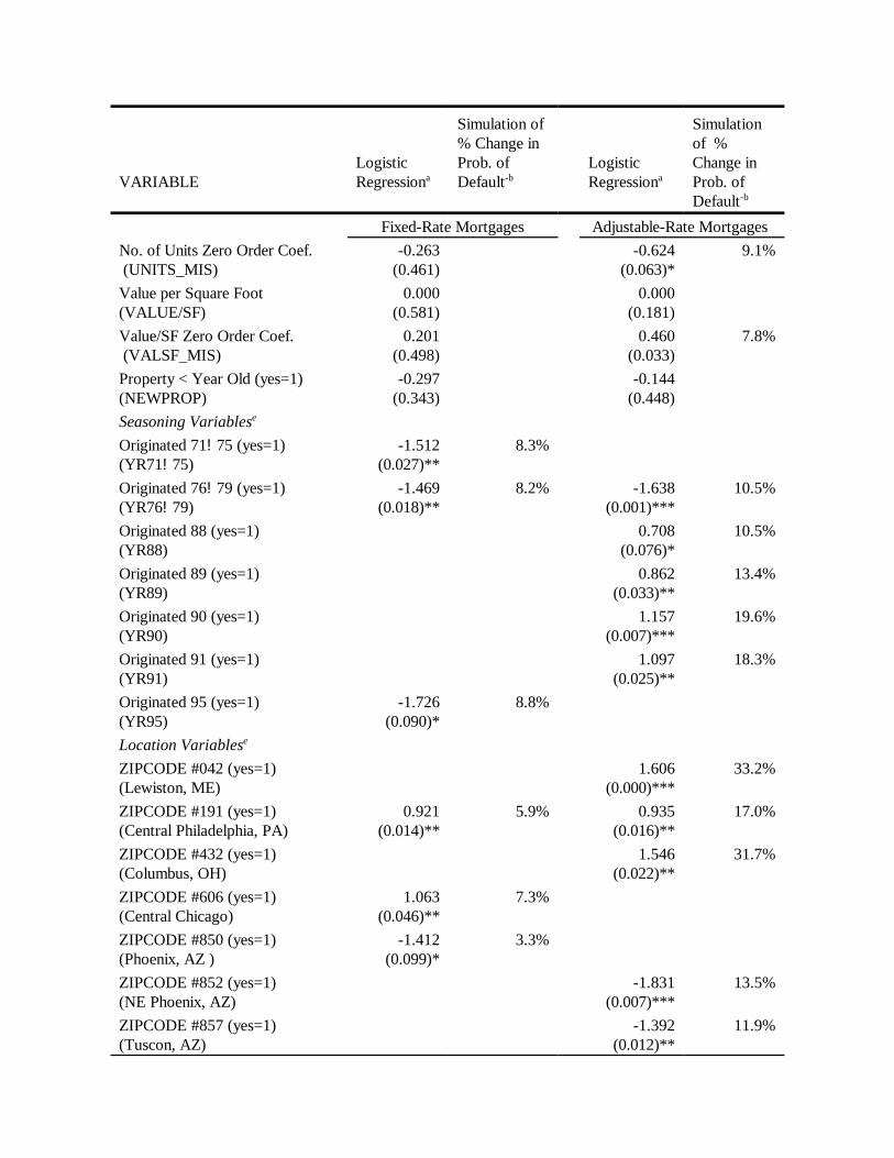
VARIABLELogisticRegressiona

Simulation of% Change inProb. ofDefault-b

LogisticRegressiona

Simulationof %Change inProb. ofDefault-b

Fixed-Rate Mortgages Adjustable-Rate Mortgages No. of Units Zero Order Coef. (UNITS_MIS)

-0.263(0.461)

-0.624(0.063)*

9.1%

Value per Square Foot(VALUE/SF)

0.000(0.581)

0.000(0.181)

Value/SF Zero Order Coef. (VALSF_MIS)

0.201(0.498)

0.460(0.033)

7.8%

Property < Year Old (yes=1)(NEWPROP)

-0.297(0.343)

-0.144(0.448)

Seasoning Variablese

Originated 71!75 (yes=1)(YR71!75)

-1.512(0.027)**

8.3%

Originated 76!79 (yes=1) (YR76!79)

-1.469(0.018)**

8.2% -1.638(0.001)***

10.5%

Originated 88 (yes=1)(YR88)

0.708(0.076)*

10.5%

Originated 89 (yes=1)(YR89)

0.862(0.033)**

13.4%

Originated 90 (yes=1)(YR90)

1.157(0.007)***

19.6%

Originated 91 (yes=1)(YR91)

1.097(0.025)**

18.3%

Originated 95 (yes=1)(YR95)

-1.726(0.090)*

8.8%

Location Variablese

ZIPCODE #042 (yes=1)(Lewiston, ME)

1.606(0.000)***

33.2%

ZIPCODE #191 (yes=1)(Central Philadelphia, PA)

0.921(0.014)**

5.9% 0.935(0.016)**

17.0%

ZIPCODE #432 (yes=1)(Columbus, OH)

1.546(0.022)**

31.7%

ZIPCODE #606 (yes=1)(Central Chicago)

1.063(0.046)**

7.3%

ZIPCODE #850 (yes=1)(Phoenix, AZ )

-1.412(0.099)*

3.3%

ZIPCODE #852 (yes=1)(NE Phoenix, AZ)

-1.831(0.007)***

13.5%

ZIPCODE #857 (yes=1)(Tuscon, AZ)

-1.392(0.012)**

11.9%

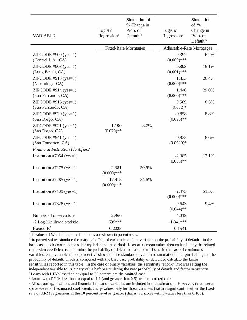
VARIABLELogisticRegressiona

Simulation of% Change inProb. ofDefault-b

LogisticRegressiona

Simulationof %Change inProb. ofDefault-b

Fixed-Rate Mortgages Adjustable-Rate Mortgages ZIPCODE #900 (yes=1)(Central L.A., CA)

0.392(0.009)***

6.2%

ZIPCODE #908 (yes=1)(Long Beach, CA)

0.893(0.001)***

16.1%

ZIPCODE #913 (yes=1)(Northridge, CA)

1.333(0.000)***

26.4%

ZIPCODE #914 (yes=1)(San Fernando, CA)

1.440(0.000)***

29.0%

ZIPCODE #916 (yes=1)(San Fernando, CA)

0.509(0.082)*

8.3%

ZIPCODE #920 (yes=1)(San Diego, CA)

-0.858(0.025)**

8.8%

ZIPCODE #921 (yes=1)(San Diego, CA)

1.190(0.020)**

8.7%

ZIPCODE #941 (yes=1)(San Francisco, CA)

-0.823(0.0089)*

8.6%

Financial Institution Identifierse

Institution #7054 (yes=1) -2.385(0.033)**

12.1%

Institution #7275 (yes=1) 2.381(0.000)***

50.5%

Institution #7285 (yes=1) -17.915(0.000)***

34.6%

Institution #7439 (yes=1) 2.473 (0.000)***

51.5%

Institution #7828 (yes=1) 0.643(0.044)**

9.4%

Number of observations 2,966 4,019-2 Log-likelihood statistic -699*** -1,841***Pseudo R2 0.2025 0.1541

a P-values of Wald chi-squared statistics are shown in parentheses.b Reported values simulate the marginal effect of each independent variable on the probability of default. In thebase case, each continuous and binary independent variable is set at its mean value, then multiplied by the relatedregression coefficient to determine the probability of default for a standard loan. In the case of continuousvariables, each variable is independently “shocked” one standard deviation to simulate the marginal change in theprobability of default, which is compared with the base case probability of default to calculate the factorsensitivities reported in this table. In the case of binary variables, the sensitivity “shock” involves setting theindependent variable to its binary value before simulating the new probability of default and factor sensitivity. c Loans with LTVs less than or equal to 75 percent are the omitted case.d Loans with DCRs less than or equal to 1.1 (and greater than 0.9) are the omitted case. e All seasoning, location, and financial institution variables are included in the estimation. However, to conservespace we report estimated coefficients and p-values only for those variables that are significant in either the fixed-rate or ARM regressions at the 10 percent level or greater (that is, variables with p-values less than 0.100).