Recursive valuation of Basket Default Swaps

Recursive valuation of Basket Default Swaps

Ian IscoeAlgorithmics Inc., 185 Spadina Avenue, Toronto, Ontario, Canada M5T 2C6

Alex KreininAlgorithmics Inc., 185 Spadina Avenue, Toronto, Ontario, Canada M5T 2C6

In this paper we consider an analytical valuation of Basket Default Swaps.Our solution is based on a continuous-time model in a conditional independenceframework. We use the order statistics of the default times of the names inthe basket to find a recursive algorithm for computation of the risk-neutraldistribution of the default process of the basket. We derive an analyticalexpression for the value of the first-to-default swap, which leads to a solutionfor an mth-to-default swap, using the recursive algorithm. The accuracy andperformance of the analytical method are compared with that obtained usingMonte Carlo simulation.

1 Introduction

In this paper we consider a simple continuous-time model for analytical val-uation of Basket Default Swaps (BDS). A BDS is a credit derivative securitywhose underlying reference assets are usually corporate bonds. The contingentpayment is triggered by a combination of default events of the reference entities.The simplest example of a BDS is the first-to-default contract under which theprotection seller is obliged to pay compensation after the first default event (if itoccurred prior to the maturity of the BDS).

Among many different models and methods proposed for analysis of basketcredit derivatives, the Gaussian multi-factor models with constant factor loadingshave become very popular (see Andersen et al. 2003; Bielecki and Rutkowski2002; Finger 2002; Huge 2002; Hull and White 2004; Kijima 2000; Kijima andMuromachi 2000; Lando 2004; Laurent 2003; Laurent and Gregory 2003; Madanet al. 2004; Schönbucher 2003). This model, with a piecewise constant hazard rateprocess, allows one to value the BDS and to compute a constant BDS premium.We find a closed-form solution for the first-to-default and for the second-to-default

We are very grateful to our colleagues Ben De Prisco, Asif Lakhany, Helmut Mausser andJennifer Lai for many comments and suggestions that helped to improve the paper. We wouldlike to thank David Lando and Brian Huge for providing us with Dr Huge’s thesis and for takingan interest in our research. We would also like to thank N. Balakrishnan for useful discussionson order statistics and in particular for the reference to his paper, cited in the bibliography.We discussed computational aspects of the recursion, proposed in this paper, with Luis Seco andDavid Saunders. Finally, we would like to thank Mark Broadie and a referee for their criticalcomments and suggestions.

95

96 I. Iscoe and A. Kreinin

contracts without assuming any homogeneity of the basket. We find a recursionfor probabilities of terminal default events1 in the basket in terms of first-to-default contracts with reduced sets of names. These default probabilities play thekey role in pricing different types of basket credit derivatives. We illustrate ourapproach by pricing mth-to-default swaps using a one-factor Gaussian model forthe conditional default probabilities.

The recursion for the probabilities of the terminal default events implies asimilar relation for the value of the BDS. Similar results for the value of a BDSwere obtained by Huge (2002) for a cumulative first-m-defaults contract usingarbitrage arguments (see also Lando (2004)).

The paper is organized as follows. In Section 2 we describe the pricing2

of a BDS and derive the main pricing equations for contracts slightly moregeneral than a BDS (this generalization includes, in particular, call and putoptions on mth-to-default losses). In Section 3 we review the model for correlateddefault events, including the specification of the default-time process and defaultintensities, to set the notation for our results. This specification allows one tocalibrate the risk-neutral default probability curves. This model is identical to thatdescribed in Andersen et al. 2003; Finger 2002; Huge 2002; Hull and White 2004;Kijima 2000; Kijima and Muromachi 2000; Lando 2004; Laurent 2003; Laurentand Gregory 2003; Madan et al. 2004; Schönbucher 2003.

Valuation of the BDS is considered in Section 4. We solve the valuationproblem explicitly for the first-to-default contract. Then we present an algorithmfor valuation of the mth-to-default contract for m > 1. The algorithm is a recursiveformula for the computation of the risk-neutral terminal default probabilities. It isimportant to mention that this recursion does not depend on the model of thedependence structure of default events; it does not even rely on the conditionalindependence framework. Calculation of the credit spread sensitivities is one ofthe most important and the most challenging problems in risk management ofportfolios of credit derivatives (Andersen et al. 2003). In Section 4.4 we brieflydiscuss the benefits of our analytical solution for BDS, for computation of theBDS sensitivities to the Credit Default Swaps (CDS) spreads.

In Section 5 we discuss performance of the recursive valuation algorithm andthe accuracy of the analytical solution described in Section 4. The paper concludeswith remarks related to the extension of the proposed approach to valuation ofmore complex credit derivatives and to future research directions.

2 Pricing equation

We consider a continuous-time model for the pricing of a BDS. Let T ={t1, t2, . . . , ti , . . . , tn = T } denote the set of premium times, with T denotingthe maturity of the swap; let t0 denote today. The basket of securities contains

1Those which trigger compensation payment.2More precisely, we price the credit-risk premium.

Journal of Computational Finance

Recursive valuation of Basket Default Swaps 97

K instruments (whose individual maturities are greater than T ). Denote by N(k)

the recovery-adjusted notional value of the kth instrument initially in the basket,k = 1, 2, . . . , K . We assume that the recovery rates are deterministic.

The buyer of protection against the mth default within the basket pays regularpremiums at the premium times ti ∈ T, (i = 1, 2, . . . , n), prior to the time ofthe mth default, expressed as an annualized rate s against a notional value N .The premium, s, is determined to balance the expected payout in the default event.

We make the following standing, financial assumptions.

(A1) There is no replacement of the underlying instruments in the basket.(A2) The premium s of the basket does not depend on time.

We consider two variants of the protection payment.

(C1) An amount of compensation is paid out at the terminal default time providedit occurs by the swap maturity.

(C2) An amount of compensation is paid out at the nearest premium datefollowing (or equal to) the terminal default time, provided it occurs by theswap maturity.

With frequent premium payments (eg, quarterly), it is most likely that defaultswill only be detected at a premium date; so (C2) is the appropriate variant in thiscase.

We also consider two variants of the premium payments.

(P1) Accrued interest is paid out at the terminal default time.(P2) No accrued interest is paid out.

The inclusion or exclusion of accrued interest is a feature of the particularcontract.

In order to mathematically express the value of the default and premium legs,for each of the variants, we introduce the following notation.

Let τ (k) denote the default time of the kth instrument (with a value +∞ ifdefault never occurs). The terminal default time, τ , triggering the compensationpayment, is a function of the random variables τ (1), τ (2), . . . , τ (K). For example,in the first-to-default contract, τ = min1≤k≤K τ(k).

For the contract variants (C2) and (P2), we introduce the notation

i(τ ) = max{i : ti < τ }and also for the variant (C2) we introduce the notation

τ ={

ti(τ )+1 if τ < T

T if τ ≥ T

Denote by L the loss of the BDS at the terminal default time:

L ={

g(N(k)) if τ = τ (k) ≤ T

0 otherwise

Volume 9/Number 3, Spring 2006


where g(·) is a payoff function. In particular, if g(x) = x and τ = min1≤k≤K τ(k),we obtain the payoff function of the first-to-default contract. If g(x) = max(x −g∗, 0) and τ is the time of the mth default, we obtain the payoff function of a calloption on the mth-to-default basket loss with the strike g∗. If g(x) = g0, and τ isthe time of the mth default, we obtain the payoff of the digital mth-to-defaultcontract.

We assume that the interest rate process is deterministic. It is not a significantloss of generality. If one assumes the hypothesis that the interest rate process isindependent of the default process of the basket, the effect of stochasticity ofinterest rates disappears.

Let D(t) = e−r(t)·(t−t0) be the discount factor corresponding to time t ; r(t)

is the risk-free interest rate corresponding to maturity t , linearly interpolatedbetween the premium dates. Thus,

r(t) = r(ti−1) + �ri

�ti(t − ti−1), ti−1 ≤ t ≤ ti

where �ri = ri − ri−1, ri = r(ti), �ti = ti − ti−1, and r(t0) is approximated bythe overnight rate. We denote the slopes of r(t) by ci :

ci = �ri

�ti, i = 1, 2, . . . , n (2.1)

We also introduce the discount factors, D(τ) and D(τ ), corresponding to thedefault time of the contract.

Throughout the paper, E denotes the risk-neutral expectation with respect toa risk-neutral probability, P. The value of the default leg in the case (C1) isE[L · D(τ)]. The value of the default leg in the case (C2) is E[L · D(τ )].The value of the premium leg in the case (P1) is E[sN ∫ τ∧T

0 D(t) dt]; in the case

(P2) the value is E[∑i(τ )i=1 s · �ti · N · D(ti)].

As in Lando (2004) and Laurent and Gregory (2003), for the purpose of numer-ical computation of the risk-neutral expectations, we introduce the probabilities

�(k)i = P(τ = τ (k), τ ∈ (ti−1, ti]), i = 1, 2, . . . , n, k = 1, 2, . . . , K (2.2)

and corresponding probability density functions, p(k)τ (t), satisfying the relation

P(τ = τ (k), τ ∈ (t, t + h]) =∫ t+h

t

p(k)τ (u) du

The following proposition is similar to the result obtained in Lando (2004) andin Laurent and Gregory (2003) for the mth-to-default contracts.

PROPOSITION 1 Under the condition (C1), the value of the default leg is

E[L · D(τ)] =K∑

k=1

g(N(k))

∫ T

0p(k)

τ (t)D(t) dt (2.3)



Under the condition (C2), it is

E[L · D(τ )] =K∑

k=1

g(N(k))

n∑i=1

D(ti)�(k)i =

n∑i=1

D(ti)

K∑k=1

g(N(k))�(k)i (2.4)

The value of the premium leg under the condition (P1) is

E

[sN

∫ τ∧T

0D(t) dt

]= sN

∫ T

0Fτ (t)D(t) dt (2.5)

where Fτ (t) = P(τ > t).Under the condition (P2), the value of the premium leg is

E

[sN

i(τ )∑i=1

�ti · D(ti)

]= sN

n∑i=1

�ti · D(ti)�i (2.6)

where the probabilities �i = P(τ > ti) satisfy the relations

�0 = 1

�i = �i−1 − �i, i = 1, 2, . . . , n

�i =K∑

k=1

�(k)i , i = 1, 2, . . . , n

The proof of Proposition 1 is straightforward and, therefore, is omitted.

REMARK. The default time, τ , can be somewhat general in Proposition 1. We needonly the following technical assumption:

the probability sample space decomposes asK⋃

k=1

{τ = τ (k) ≤ T } ∪ {τ > T }

(the event, {τ > T }, is the possibility that no compensation is ever paid).

3 Conditional independence framework

In this section we review the conditional independence framework based on amulti-factor Gaussian model with constant factor loadings.

3.1 Conditional default probabilities

Denote the risk-neutral, cumulative default probabilities of the kth name byπ (k)(t):

P(τ (k) ≤ t) = π (k)(t), k = 1, 2, . . . , K

Let X denote the vector of jointly normally distributed credit drivers X := (X1,

. . . , XC) with each Xc standardized and denote by R the correlation matrix of X.



Let x = (x1, . . . , xC) be a particular value of X. The conditional risk-neutraldefault probabilities are given by

π (k)(t, x) = �

([�−1(π (k)(t)) −

C∑c=1

β(k)c xc

]/σ (k)

)(3.1)

where � denotes the standard normal cumulative distribution function, and thecoefficients β

(k)c and σ (k) satisfy the relation

(σ (k))2 +C∑

c=1

C∑c′=1

β(k)c Rcc′β(k)

c′ = 1

for each k = 1, 2, . . . , K .In this framework, the default events of the names are conditionally indepen-

dent. This assumption allows us to reduce the problem of computation of thedensities p

(k)τ (·) in Proposition 1 to the case of independent names. The latter

satisfy the relation

p(k)τ (t) =

∫RC

p(k)τ (t, x) dϕ(x), k = 1, 2, . . . , K (3.2)

where p(k)τ (t, x) denotes the conditional density conditioned on X = x (ie, with

default probabilities given by (3.1)) and ϕ is the joint distribution of the creditdrivers.

We denote by Px the risk-neutral probability measure, conditional on X = x.

3.2 Default intensities

The conditional probability distribution function of τ (k) can be represented in theform

F(k)(t, x) ≡ Px(τ(k) ≤ t) = 1 − exp(−(k)(t, x))

where (k)(t, x) = ∫ t

t0λ(k)(u, x) du and the function λ(k)(·) is the conditional

default intensity of the kth name.The unconditional distribution of the default time of the kth name can be deter-

mined from the CDS credit spread quotes having maturities among t1, t2, . . . , tn.Let π

(k)i be the cumulative unconditional risk-neutral probability of default of

the kth name by time ti : π(k)i = P(τ (k) ≤ ti ), i = 1, 2, . . . , n. Using (3.1) we

compute the conditional risk-neutral default probabilities, π(k)i (x) at t = ti , and

set F(k)(ti, x) to be the latter, for i = 1, 2, . . . , n, in a given scenario, x, so thatPx(τ

(k) ≤ ti ) = π(k)i (x).

The function (k)(t, x) satisfies the equation

(k)(ti, x) = −ln π(k)i (x), k = 1, 2, . . . , K, i = 1, 2, . . . , n

where π(k)i (x) = 1 − π

(k)i (x). Since (k)(t, x) is determined only at times ti , we

have to interpolate the values of (k)(t, x) to compute it at an arbitrary value of t .



If we choose linear interpolation, then λ(k)(t, x) is a piecewise constant function:

λ(k)(t, x) = λ(k)i (x) for t ∈ (ti−1, ti]

Then we obtain that, for i = 1, 2, . . . , n,

λ(k)i (x) = 1

�tilog

(π

(k)i−1(x)

π(k)i (x)

)where �ti = ti − ti−1 (3.3)

Linear interpolation of (k)(t, x) is not the only way to construct the functionλ(k)(t, x). An alternative method of continuation can be based on linearinterpolation of the distribution function F(k)(t, x), which has the followingremarkable property: it maximizes the entropy of the random variable τ (k).Any choice of interpolation introduces a numerical (as opposed to financial)approximation because conditional and unconditional default probabilities cannotbe set arbitrarily and remain probabilistically consistent. In this paper we adoptlinear interpolation.

4 Valuation of BDS

In this section we continue the evaluations of the right-hand sides of (2.2)–(2.6),in the setting of Section 3.

Let τ1 < τ2 < · · · < τK be the order statistics of the default times3

τ1 = min1≤k≤K

τ(k),

τ2 = min1≤k≤K

{τ (k) : τ (k) > τ1}, . . .

. . . , τm = min1≤k≤K

{τ (k) : τ (k) > τm−1}, . . . , τK = max1≤k≤K

τ(k)

If the BDS is structured as an mth-to-default contract, the default time τ ≡ τm isthe mth of the order statistics of τ (k) (k = 1, 2, . . . , K).

4.1 First-to-default contract

In this case τ ≡ τ1 = min1≤k≤K τ(k).To formulate the result for the first-to-default contract we introduce the special

functions Daw± , usually called Dawson’s integrals:4

Daw+(u) = e−u2∫ u

0ev2

dv

Daw−(u) = eu2∫ u

0e−v2

dv

3Note that the default times τ (k) are distinct almost surely. For this reason, the definition of theorder statistics requires strict inequality.4The properties of the Dawson’s integrals can be found in Abramovitz and Stegun (1972) andSpanier and Oldham (1987).



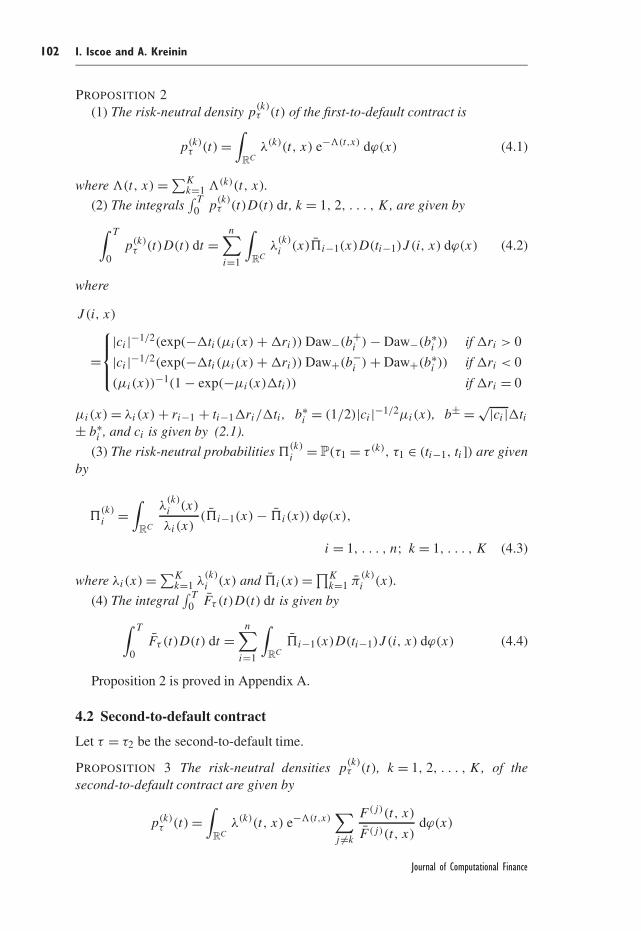
PROPOSITION 2(1) The risk-neutral density p

(k)τ (t) of the first-to-default contract is

p(k)τ (t) =

∫RC

λ(k)(t, x) e−(t,x) dϕ(x) (4.1)

where (t, x) = ∑Kk=1 (k)(t, x).

(2) The integrals∫ T

0 p(k)τ (t)D(t) dt , k = 1, 2, . . . , K , are given by∫ T

0p(k)

τ (t)D(t) dt =n∑

i=1

∫RC

λ(k)i (x)�i−1(x)D(ti−1)J (i, x) dϕ(x) (4.2)

where

J (i, x)

=

|ci |−1/2(exp(−�ti(µi(x) + �ri)) Daw−(b+

i ) − Daw−(b∗i )) if �ri > 0

|ci |−1/2(exp(−�ti(µi(x) + �ri)) Daw+(b−i ) + Daw+(b∗

i )) if �ri < 0

(µi(x))−1(1 − exp(−µi(x)�ti)) if �ri = 0

µi(x) = λi(x) + ri−1 + ti−1�ri/�ti , b∗i = (1/2)|ci|−1/2µi(x), b± = √|ci |�ti

± b∗i , and ci is given by (2.1).

(3) The risk-neutral probabilities �(k)i = P(τ1 = τ (k), τ1 ∈ (ti−1, ti]) are given

by

�(k)i =

∫RC

λ(k)i (x)

λi(x)(�i−1(x) − �i(x)) dϕ(x),

i = 1, . . . , n; k = 1, . . . , K (4.3)

where λi(x) = ∑Kk=1 λ

(k)i (x) and �i(x) = ∏K

k=1 π(k)i (x).

(4) The integral∫ T

0 Fτ (t)D(t) dt is given by∫ T

0Fτ (t)D(t) dt =

n∑i=1

∫RC

�i−1(x)D(ti−1)J (i, x) dϕ(x) (4.4)

Proposition 2 is proved in Appendix A.

4.2 Second-to-default contract

Let τ = τ2 be the second-to-default time.

PROPOSITION 3 The risk-neutral densities p(k)τ (t), k = 1, 2, . . . , K, of the

second-to-default contract are given by

p(k)τ (t) =

∫RC

λ(k)(t, x) e−(t,x)∑j �=k

F (j)(t, x)

F (j)(t, x)dϕ(x)



The risk-neutral probabilities �(k)i are given by

�(k)i =

∫RC

∑1≤j≤K

j �=k

Qkj (i, x) dϕ(x), k = 1, 2, . . . , K, i = 1, 2, . . . , n (4.5)

where

Qkj (i, x) = λ

(k)i (x)

λi(x) − λ(j)

i (x)(�

i−1(x) − �

i (x))

− λ(k)i (x)

λi(x)(�i−1(x) − �i(x)) (4.6)

and

�

i (x) =∏

1≤k≤Kk �=j

π(k)i (x), λi(x) =

K∑k=1

λ(k)i (x)

Using Equations (2.4), (2.6), (4.5) and (4.6), we can find simple expressionsfor the risk-neutral credit-risk premium or the value of the second-to-defaultcontract of variant (C2) and (P2). For other variants, one can use Proposition 2and Theorem 1 of the next section, but the resulting expressions are complicatedand therefore not detailed here.

Proposition 3 is a corollary of Proposition 2 and Theorem 1 in the next section.The structure of the expression for the probabilities Qk

j (i, x) in Proposition 3reveals that the computation of the probabilities, �

(k)i , for the second-to-default

contract is reduced to computation of the probabilities �(k)i for the first-to-default

contract on two types of baskets: (i) B , (j = 1, 2, . . . , K, j �= k) containing allbut the j th name from the original basket; and (ii) the original basket. We makedirect use of this idea in handling the general case of an mth-to-default contract inthe next section.

4.3 Valuation of mth-to-default contract

We first derive a recurrence relation (in m) for the risk-neutral probabilitydensities, p

(k)τm , and the risk-neutral probabilities, �

(k)i , associated with the mth-

to-default BDS, for m ≥ 2.Let us introduce again the modified basket, B , containing all but the j th

name from the original basket. Denote by τm

(B)

the mth-to-default time inthe basket B .

We use the notation p(k)m (t; B) for the risk-neutral density p

(k)τm (t; B) in the orig-

inal basket, and the notation p(k)m (t; B ) for the risk-neutral density p

(k)τm (t; B )

in the basket B .



THEOREM 1 The risk-neutral densities p(k)m (t; B ) and p

(k)m−1(t; B ) satisfy the

relation

(m − 1)p(k)m (t; B ) =

∑j �=k

p(k)m−1(t; B ) − (K − m + 1)p

(k)m−1(t; B ) (4.7)

Theorem 1 is proved in Appendix B.Let us also introduce the probabilities Pm(B) = P(τm = τ (k), τm ∈ (ti−1, ti])

in the original basket, and the probabilities Pm(B ) = P(τm(B ) = τ (k), τm ∈(ti−1, ti]) in the basket B . Note that Pm is the same as �

(k)i for the mth-to-default

contract, but when k and i are fixed, we use the former notation to focus on thevariable parameter, m, and also the choice of the basket, B or B .

Denote Fτm(t; B) = P(τm > t) in the original basket, and Fτm(t; B ) =P(τm > t) in the basket B .

The following corollary is immediate from Theorem 1.

COROLLARY 1 The probabilities Pm(B) and Pm(B ) satisfy the relation

(m − 1)Pm(B) =∑j �=k

Pm−1(B ) − (K − m + 1)Pm−1(B), m = 2, 3, . . . , K (4.8)

The integrals I(k)m (B) = ∫ T

0 p(k)τm (t; B)D(t) dt , k = 1, 2, . . . , K , satisfy the

recursion

(m − 1)I (k)m (B) =

∑j �=k

I(k)m−1(B ) − (K − m + 1)I

(k)m−1(B) (4.9)

The integrals Im(B) = ∫ T

0 Fτm(t; B)D(t) dt satisfy the same relation (4.9) with

I substituted for I (k).

Theorem 1 and Corollary 1 allow us to compute recursively the risk-neutraldefault probabilities and expectations for the mth-to-default BDS, from which wecan then find the risk-neutral credit-risk premium or the value of the contract,using the results (2.3)–(2.6). When the recursion arrives at m = 1, we can useProposition 2 to finish computation.

REMARK. The recursion in Theorem 1 does not depend explicitly on the choice ofinterpolation used to construct the default distributions, F(k), nor does it dependon the conditional independence assumption. The latter follows from the proofin Appendix B. This is useful for implementations, as Theorem 1 is valid form = 2, so that only the simplest case of the first-to-default BDS need be workedout in detail (although performance must also be considered). For the first-to-default BDS, the choice of interpolation must come into play; and it is for thefirst-to-default BDS result that we have used the conditional independence.



It is at least of theoretical interest to find an explicit expression that reducesthe general case down to the case of first-to-default contracts. To do that, we mustgeneralize our notation for reduced baskets.

With the names in the original basket enumerated by K = {1, 2, . . . , K}, foreach subset J ⊂ K, we let |J | denote the number of names in J. Denote by BJ ,

the reduced basket obtained by omitting from B, the names in J. When |J | = 1,with say J = {j}, then BJ is simply B . When |J | = 0, ie, when J is empty,BJ ≡ B. The complete reduction for the probabilities Pm(B) can now beexpressed as

Pm(B) =m−1∑ν=0

(−1)m−ν−1(

K − ν − 1

m − ν − 1

) ∑J⊂K:|J |=ν

P1(BJ ) (4.10)

This result follows from Theorem 1, by induction on m.Naive implementation of recursion (4.8) leads to recalculation of the same

probabilities many times for m > 2. Therefore, it is recommended to cache theresults or, alternatively, to implement (4.10) for which there is no redundancy.

4.4 Computation of sensitivities

In this section we address the problem of computation of sensitivities (greeks)for a BDS, ie, the partial derivatives of the value function, V , with respect to thebasic parameters, on which it depends. In order to make the discussion reasonablygeneral but also explicit, we shall restrict our attention to those parameters thatinfluence the conditional default probabilities, π

(k)i (x). These parameters are the

factor loadings (β(k)), the volatilities (σ (k)), and the par CDS credit spreads (s(k)i )

which determine the unconditional default probabilities from the bootstrappeddefault intensity. (Thus we are excluding the recovery rates, the risk-neutralinterest rates, and the time to maturity, but only for the sake of concreteness.There is no essential difficulty in handling them.) Sensitivities to the par CDScredit spread quotes are perhaps the most complex and perhaps also of thegreatest interest. We denote by θ any one of the scalar parameters that we areconsidering.

Having analytic solutions for the valuation of a BDS reduces the computationof sensitivities to nothing more than a lengthy exercise in differential calculus.This approach is described in general terms in Andersen et al. (2003), which wemake more explicit for our results.

There are two key aspects of the computation for an mth-to-default contract:(i) a constant-coefficient, linear recursion for m > 1; and (ii) an explicit resultfor m = 1. These two aspects apply not only for valuation; they can be usedin exactly the same way for the computation of sensitivities. Indeed, the linearrecursion(s) for the case of an mth-to-default contract (see Corollary 1), canbe differentiated with respect to the parameter, θ , yielding recursions required



for the desired sensitivity – recursions of the same algebraic form as theundifferentiated ones. In particular, the problem is reduced to that for a first-to-default contract, for which we have an explicit result for differentiation– see Propositions 1 and 2. Together with (3.1), those results show that, intaking the derivative, ∂/∂θ , we can apply the chain rule, going through theintermediate variables, π

(k)i (x). In other words, the formula for the value of a

first-to-default contract is of the form,∫RC G(x) dϕ(x), where G is an alge-

braic function (including an exponential composite) of the variables, π(k)i (x).

Thus we obtain the desired sensitivity as∫RC

∑k,i

∂G(x)

∂[π (k)i (x)]

∂π(k)i (x)

∂θdϕ(x)

where the partials, ∂G(x)/∂[π (k)i (x)], will be explicit. The quantities ∂π

(k)i (x)/∂θ

are calculated with the chain rule applied to (3.1). For θ being one of thefactor loadings or volatilities, the latter derivatives are explicit and thereforeimmediate. In the case that θ is one of the par CDS credit spread quotes, θ

appears only implicitly in π(k)i (x), through �−1(π

(k)i ): for each name k, π

(k)i =

1 − exp(− ∫ tit0

λ(k)(t) dt); and λ(k)(t) is piecewise constant and bootstrapped fromthe par CDS credit spread quotes in the usual way. Suppose we have B spreadquotes, (sb)

Bb=1, corresponding to maturities (Tb)

Bb=1. (With k fixed, we suppress

it from the notation.) Denoting the theoretical value of the bth CDS by Vb, we havethe following system of equations for (λb)

Bb=1, λb being the constant value of λ(t)

for t in (Tb−1, Tb]:0 = V1(λ1; s1) ⇒ λ1 ≡ λ1(s1)

0 = V2(λ1, λ2; s2) ⇒ λ2 ≡ λ2(s1, s2)

...

0 = VB(λ1, . . . , λB; sB) ⇒ λB ≡ λB(s1, . . . , sB)

from which it follows by implicit differentiation that, for 1 ≤ b ≤ B and1 ≤ j < b,

∂λb

∂sb= − ∂Vb/∂sb

∂Vb/∂λb

∂λb

∂sj= −

b−1∑�=j

(∂Vb/∂λ�)(∂λ�/∂sj )

∂Vb/∂λb

The quantities ∂G(x)/∂[π (k)i (x)] are common to large parts of these computa-

tions, and can be precalculated for use with all θs of interest. For credit-spreadsensitivities, the partials, ∂Vb/∂λ�, 1 ≤ � ≤ b, are common to all computations,∂λb/∂sj .



TABLE 1 Parameters of the BDS.

Name Notional Credit rating Correlation

1 190 C7 0.52 80 C2 0.63 70 C4 0.94 360 C6 0.65 100 C5 0.56 200 C6 0.47 150 C6 0.78 123 C5 0.649 95 C6 0.55

10 107 C3 0.22

5 Accuracy and performance

In this section we compare the accuracy and performance of Monte Carlosimulation of BDS with that of the analytical solution. All examples follow thecontract variant with the assumptions (C2) and (P2).

The method of valuation of BDS contracts invokes numerical integrationin Equations (4.2)–(4.5). Clearly the computation time is proportional to thenumber of points in the numerical quadrature. In the context of risk management,where each BDS will be valued under thousands of scenarios, the choice ofnumerical quadrature becomes important. An optimal choice of the numericalquadrature depends on the type of the model describing the joint distribution ofdefault times. Both the Gauss–Legendre quadrature and the Hermite quadratures(Press et al. 2002) can be used for pricing BDS in the Gaussian one-factor andmulti-factor models.

In our numerical experiments, we used the Gaussian one-factor model for thejoint distribution of default times. We also used a special quadrature originallydesigned for pricing of interest rate derivatives (Curran 2001). It performs well inthe computation of Gaussian integrals and often outperforms the Gauss–Legendreand Hermite quadratures.

5.1 Accuracy

The first basket used in our numerical experiments contains 10 names with theparameters shown in Table 1. This BDS has an inhomogeneous structure: all theinstruments in the basket have different notionals as well as different correlationsβ(k) with the credit driver and different risk-neutral default probability curves.The maturity of the BDS is 5 years and ti = i, (i = 1, 2, 3, 4, 5). The recoveryrates in the basket are 15%. The interest rate curve (rates are continuouslycompounded) is

r(t1) = 0.046, r(t2) = 0.05, r(t3) = 0.056, r(t4) = 0.058, r(t5) = 0.06



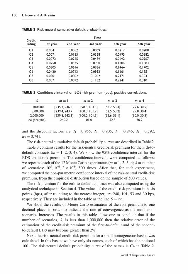
TABLE 2 Risk-neutral cumulative default probabilities.

TimeCreditrating 1st year 2nd year 3rd year 4th year 5th year

C1 0.0041 0.0052 0.0069 0.0217 0.0288C2 0.0071 0.0185 0.0328 0.0495 0.0682C3 0.0072 0.0225 0.0439 0.0692 0.0967C4 0.0258 0.0575 0.0930 0.1304 0.1683C5 0.0305 0.0616 0.0936 0.1464 0.1702C6 0.0420 0.0713 0.0953 0.1661 0.195C7 0.0501 0.0802 0.1062 0.2171 0.303C8 0.0571 0.0872 0.1132 0.2241 0.310

TABLE 3 Confidence interval on BDS risk premium (bps): positive correlations.

S m = 1 m = 2 m = 3 m = 4

100,000 [235.3, 246.5] [98.3, 103.3] [52.2, 53.4] [29.6, 30.5]1,000,000 [239.4, 243.7] [100.0, 101.7] [52.5, 53.2] [29.8, 30.4]2,000,000 [239.8, 242.1] [100.0, 101.5] [52.6, 53.1] [30.0, 30.3]

∞ (analytic) 240.2 101.0 52.8 30.2

and the discount factors are d1 = 0.955, d2 = 0.905, d3 = 0.845, d4 = 0.792,d5 = 0.741.

The risk-neutral cumulative default probability curves are described in Table 2.Table 3 contains results for the risk-neutral credit-risk premium for the mth-to-

default contracts (m = 1, 2, 3, 4). We show the 95% confidence interval for theBDS credit-risk premium. The confidence intervals were computed as follows:we repeated each of the 12 Monte Carlo experiments (m = 1, 2, 3, 4; S = numberof scenarios: 105, 106, 2 × 106) 500 times. After that, for each experiment,we computed the non-parametric confidence interval of the risk-neutral credit-riskpremium, from the empirical distribution based on the sample of 500 values.

The risk premium for the mth-to-default contract was also computed using theanalytical technique in Section 4. The values of the credit-risk premium in basispoints (bps), after rounding to the nearest integer, are 240, 101, 53 and 30 bps,respectively. They are included in the table as the line S = ∞.

We show the results of Monte Carlo estimation of the risk premium to onedecimal place, in order to indicate the rate of convergence as the number ofscenarios increases. The results in this table allow one to conclude that if thenumber of scenarios, S, is less than 1,000,000 then the relative error of theestimation of the credit-risk premium of the first-to-default and of the second-to-default BDS may become greater than 2%.

Next, the risk-neutral credit-risk premium for a small homogeneous basket wascalculated. In this basket we have only six names, each of which has the notional100. The risk-neutral default probability curve of the names is C4 in Table 2.



TABLE 4 Confidence interval on BDS risk premium (bps): signed correlations.

S m = 1 m = 2 m = 3 m = 4

100,000 [222.9, 232.1] [98.1, 104.5] [43.9, 45.2] [0, 0.1]1,000,000 [226.2, 229.6] [100.0, 102.4] [44.2, 44.9] [0, 0]4,000,000 [227.0, 228.6] [100.6, 102.1] [44.3, 44.8] [0, 0]

∞ (analytic) 227.6 101.3 44.6 0

The names in the basket have the following correlations with the credit driver:

β(1) = −0.94, β(2) = 0.92, β(3) = 0.91

β(4) = −0.87, β(5) = 0.85, β(6) = −0.79

Thus, the names in the basket are split into two subgroups (according to thesign of β), both having strong correlations with the credit driver. The maturityof each of the contracts is 5 years. The discount curve and premium dates in thisexperiment are the same as in the previous one.

Table 4 contains the results of Monte Carlo simulation of the risk-neutral credit-risk premium for four mth-to-default contracts (m = 1, 2, 3, 4). Again, the resultswould be rounded to the nearest integer in practice.

In this case, the analytical values of the credit-risk premium are: 228 bps for thefirst-to-default contract; 101 bps for the second-to-default contract; 45 bps for thethird-to-default contract. Since the probability of four defaults during the lifetimeof the contract is very small, the risk-neutral credit-risk premium for the fourth-to-default contract is zero after rounding. (Four defaults entails the same behaviorbetween two highly negatively correlated groups.) Again, the relative error in theMonte Carlo estimation of the credit-risk premium may become greater than 2%if the number of scenarios S < 1,000,000.

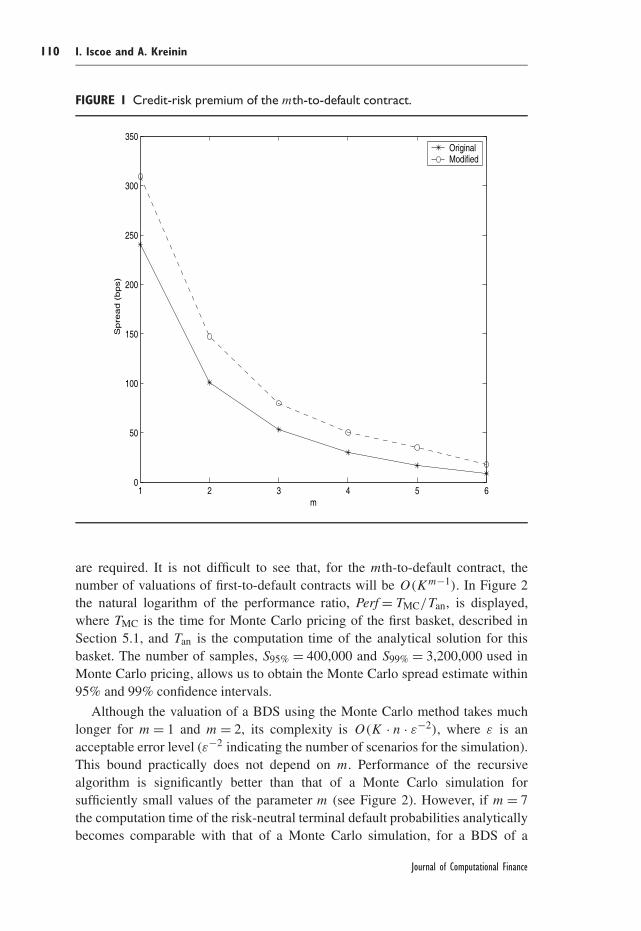
Figure 1 represents the credit-risk premiums of the mth-to-default contract as afunction of m. The first (solid) curve is the credit-risk premiums of the first BDS,described in this section. The second curve represents the credit-risk premiumsof the contracts having the same notionals and the same correlation coefficients,β(k) but with the risk-neutral default probabilities of the names increased asfollows: if the default probability curve of a name is Cj in the original basket thenin the modified basket this name will be attached to the curve Cj+1. The results inFigure 1 demonstrate that in this case the credit-risk premium sensitivity (relativedifference) of the mth-to-default contract is a monotonically increasing functionof the parameter m.

5.2 Performance of recursive algorithm

The algorithm described in Theorem 1 has a combinatorial nature. Indeed,to compute the risk-neutral default probabilities for the second-to-default contract,K valuations of first-to-default contracts on K baskets, B (j = 1, 2, . . . , K),



FIGURE 1 Credit-risk premium of the mth-to-default contract.

1 2 3 4 5 60

50

100

150

200

250

300

350

m

Spre

ad (

bps)

OriginalModified

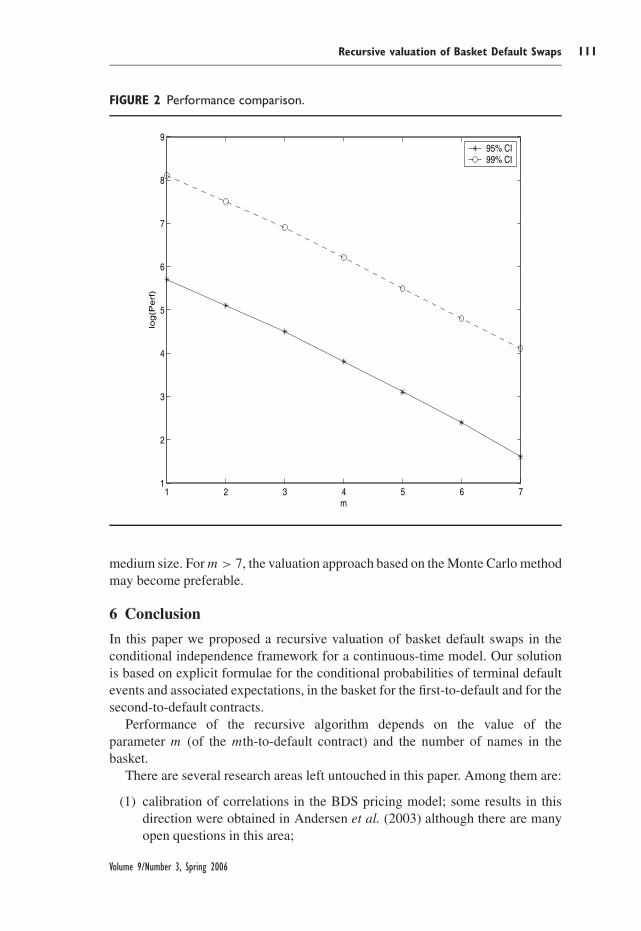
are required. It is not difficult to see that, for the mth-to-default contract, thenumber of valuations of first-to-default contracts will be O(Km−1). In Figure 2the natural logarithm of the performance ratio, Perf = TMC/Tan, is displayed,where TMC is the time for Monte Carlo pricing of the first basket, described inSection 5.1, and Tan is the computation time of the analytical solution for thisbasket. The number of samples, S95% = 400,000 and S99% = 3,200,000 used inMonte Carlo pricing, allows us to obtain the Monte Carlo spread estimate within95% and 99% confidence intervals.

Although the valuation of a BDS using the Monte Carlo method takes muchlonger for m = 1 and m = 2, its complexity is O(K · n · ε−2), where ε is anacceptable error level (ε−2 indicating the number of scenarios for the simulation).This bound practically does not depend on m. Performance of the recursivealgorithm is significantly better than that of a Monte Carlo simulation forsufficiently small values of the parameter m (see Figure 2). However, if m = 7the computation time of the risk-neutral terminal default probabilities analyticallybecomes comparable with that of a Monte Carlo simulation, for a BDS of a



FIGURE 2 Performance comparison.

1 2 3 4 5 6 71

2

3

4

5

6

7

8

9

m

log

(Pe

rf)

95% CI99% CI

medium size. For m > 7, the valuation approach based on the Monte Carlo methodmay become preferable.

6 Conclusion

In this paper we proposed a recursive valuation of basket default swaps in theconditional independence framework for a continuous-time model. Our solutionis based on explicit formulae for the conditional probabilities of terminal defaultevents and associated expectations, in the basket for the first-to-default and for thesecond-to-default contracts.

Performance of the recursive algorithm depends on the value of theparameter m (of the mth-to-default contract) and the number of names in thebasket.

There are several research areas left untouched in this paper. Among them are:

(1) calibration of correlations in the BDS pricing model; some results in thisdirection were obtained in Andersen et al. (2003) although there are manyopen questions in this area;



(2) analysis and valuation of BDS options;(3) extension of the approach to stochastic recoveries and a random interest rate

process.

Our approach to pricing of BDS contracts can be significantly generalizedto more complex contracts including options on basket losses and Asian-typeoptions. These are directions for future research.

Appendix A Proof of Proposition 2

Equation (4.1) for the density can be found in Lando (2004).Consider the conditional probability density function, q(k)(t, x), of the random

variable τ (k). We have

q(k)(t, x) = ∂(k)(t, x)

∂texp(−(k)(t, x)), k = 1, 2, . . . , K (A.1)

The conditional probability that the index of the first-to-default name is k and thedefault time τ1 ∈ (ti−1, ti] is

�(k)i (x) ≡ Px(τ1 = τ (k) ∈ (ti−1, ti])

=∫ ti

ti−1

q(k)(t, x)Px

(mink′ �=k

τ (k′) > t

)dt

=∫ ti

ti−1

q(k)(t, x)∏k′ �=k

exp(−(k′)(t, x)) dt (A.2)

From (A.1) and (A.2) we obtain

�(k)i (x) =

∫ ti

ti−1

∂(k)(t, x)

∂texp(−(t, x)) dt (A.3)

where (t, x) = ∑Kk=1 (k)(t, x). The function (t, x) satisfies the equation

(t, x) = (ti−1, x) + λi(x) · (t − ti−1), t ∈ (ti−1, ti] (A.4)

where λi(x) = ∑Kk=1 λ

(k)i (x).

Denote �i(x) = Px(τ1 > ti). Then we have

�i(x) =K∏

k=1

π(k)i (x) = exp(−(ti, x))

The latter relation, (A.3) and (A.4) yield

�(k)i (x) = λ

(k)i (x)�i−1(x)

∫ ti

ti−1

exp(−λi(x)(t − ti−1)) dt (A.5)



and, finally,

�(k)i (x) = λ

(k)i (x)

λi(x)[�i−1(x) − �i(x)] (A.6)

Equation (4.3) follows from (A.6) by integrating. The proof of (4.2) is similarto that of (4.3): starting from Equation (3.2), one reduces the calculation to∫ T

0p(k)

τ (t, x)D(t) dt =n∑

i=1

λ(k)i (x)�i−1(x)D(ti−1)

×∫ ti

ti−1

exp(λi(x)(t − ti−1)) exp(−ci · t · (t − ti−1)) dt

which follows in the same way as was done for (A.5). The rest is calculus.Proof of (4.4) goes along the same lines as those for (4.2), starting from the

representation∫ T

0Fτ (t)D(t) dt =

∫RC

dϕ(x)

n∑i=1

∫ ti

ti−1

e−(t,x)D(t) dt �

Appendix B Proof of Theorem 1

Theorem 1 follows immediately from a very general result on order statistics,which we first establish.

Let (�, F, P) be a probability space and let A1, . . . , An be n events. For 1 ≤r ≤ n, denote by �r and Pr , the probabilities

�r = P(exactly r of the Aj occur)

Pr = P(at least r of the Aj occur)

so that

Pr =n∑

R=r

�R, 1 ≤ r ≤ n

�r = Pr − Pr+1, 1 ≤ r ≤ n − 1 (B.1)

We similarly denote by �[i]r and P [i]

r the probabilities corresponding to thereduced list of n − 1 events, obtained by omitting Ai from the original list,A1, . . . , An. The indicator technique used by Balasubramanian and Balakrishnanto prove their theorem in Balasubramanian and Balakrishnan (1992) can also beused to establish the following more general result. (Indeed, the proof essentiallyfollows verbatim their proof, with only a small change in notation: replace theirF with our P. See also the Remark at the end of this appendix, for an alternativeapproach.)



THEOREM 2 For 1 ≤ r ≤ n − 1,

(r + 1)�r+1 + (n − r)�r =n∑

i=1

�[i]r (B.2)

rPr+1 + (n − r)Pr =n∑

i=1

P [i]r (B.3)

The result in Balasubramanian and Balakrishnan (1992) is a special case ofthis theorem, corresponding to the choice Aj = {Xj ≤ x}, where X1, . . . , Xn

are random variables on � and x is any fixed real number. Continuing with thisnotation, we let Xr:n denote the rth-order statistic from this family of randomvariables, and X

[i]r:n the rth-order statistic from the same family but with Xi

omitted. The following corollary generalizes the result in Balasubramanian andBalakrishnan (1992), in the case where the joint distribution of the randomvariables is continuous, so that we may speak of the rth-order statistic coincidingwith one of the original random variables.

COROLLARY 2 Assuming that the joint distribution of the random variablesX1, . . . , Xn is continuous, the following identity holds for 1 ≤ r ≤ n − 1, 1 ≤k ≤ n, and x ∈ R:

rP(Xr+1:n = Xk ≤ x) + (n − r)P(Xr:n = Xk ≤ x)

=∑

1≤i≤n,i �=k

P(X[i]r:n = Xk ≤ x)

PROOF. If P(Xk ≤ x) = 0, then the corollary is trivial; so we assume other-wise and apply the identity (B.2) of Theorem 2 to the probability measure,P(· | Xk ≤ x), and the events Aj = {Xj ≤ Xk}. The corollary then follows fromthe following three observations:

(1) the two events, {exactly r Xj ’s ≤ Xk} and {Xr:n = Xk}, coincide;(2) for i �= k, {exactly r Xj ’s (j �= i) ≤ Xk} = {X[i]

r:n = Xk};(3) {exactly r Xj ’s (j �= k) ≤ Xk} = {Xr+1:n = Xk}; so �

[k]r = �r+1. �

PROOF OF THEOREM 1. We need only make the following identifications inCorollary 2:

n = K, i = k, r = m − 1, Xj = τ (j), x = t

and then differentiate with respect to t . (For (4.8) in Corollary 1, one can directlytake a difference, in Corollary 2, at the two times ti−1, ti in (2.2).) �

REMARK. The identity (B.3) in Theorem 2 can be completely reduced to thefollowing form:

Pr =r−1∑ν=0

(−1)r−ν−1(n − ν − 1

r − ν − 1

) ∑|J |=ν

P [J ]1 (B.4)



where J ranges over subsets of {1, 2, . . . , n}, |J | denotes the number of elementsin J , and P [J ]

1 denotes the probability of occurrence of at least one of the eventsA1, A2, . . . , An, other than (Aj)j∈J . Consequently, by (B.1),

�r =r∑

ν=0

(−1)r−ν−1(

n − ν

r − ν

) ∑|J |=ν

P [J ]1 (B.5)

Identities of the type (B.2), (B.3), (B.4) and (B.5) are a subject unto themselves.The interested reader may consult Rényi (1970, Section 2.6). In particular, theidentity (2.6.23) therein, due to Jordan, is a different (unreduced) version of (B.5).An alternative proof of Theorem 2 can be based on Rényi (1970, Theorem 2.6.1).

REFERENCES

Abramovitz, M., and Stegun, I. (1972). Handbook of Mathematical Functions with Formulas,Graphs and Mathematical Tables, 9th edn. Dover, New York.

Andersen, L., Sidenius, J., and Basu, S. (2003). All your hedges in one basket. RISK 16(11),67–72.

Balasubramanian, K., and Balakrishnan, N. (1992). Indicator method for a recurrence relationfor order statistics. Statistics and Probability Letters 14, 67–69.

Bielecki, T. R., and Rutkowski, M. (2002). Credit Risk: Modeling, Valuation and Hedging.Springer, Berlin.

Curran, M. (2001). Willow power: optimizing derivatives pricing trees. Algo ResearchQuarterly 4(4), 15–23.

Finger, C. (2002). Closed-form Pricing of Synthetic CDO’s and Applications. ICBI RiskManagement, Geneva, December 2002.

Huge, B. (2002). On defaultable claims and credit derivatives. PhD Thesis, Department ofStatistics and Operations Research, University of Copenhagen.

Hull, J., and White, A. (2004). Valuation of a CDO and an nth to default CDS without MonteCarlo simulation. Journal of Derivatives 12(2), 8–23.

Kijima, M. (2000). Valuation of credit swap of the basket type. Review of Derivatives Research4, 81–97.

Kijima, M., and Muromachi, Y. (2000). Credit events and the valuation of credit derivatives ofbasket type. Review of Derivatives Research 4, 55–79.

Lando, D. (2004). Credit Risk Modeling: Theory and Applications. Princeton University Press,Princeton.

Laurent, J.-P. (2003). Accurately Valuing Basket Default Swaps and CDO’s using Factor Models(Quant’03). London, September (http://www.defaultrisk.com).

Laurent, J.-P., and Gregory, J. (2003). Basket default swaps, CDO’s and factor copulas. WorkingPaper, 21 pp. (http://www.defaultrisk.com).

Madan, D., Konikov, M., and Marinescu, M. (2004). Credit and basket default swaps, RobertH. Smith School of Business and Bloomberg L. P. Working Paper, 23 pp.(http://www.defaultrisk.com).



Press, W., Teukolsky, S, Vetterling, W., and Flannery B. (2002). Numerical Recipes in C++:The Art of Scientific Computing. Cambridge University Press, Cambridge.

Rényi, A. (1970). Foundations of Probability. Holden-Day, San Francisco, CA.

Schönbucher, P. (2003). Credit Derivatives Pricing Models: Models, Pricing and Implementa-tion. Wiley, Chichester.

Spanier, J., and Oldham, K. (1987). An Atlas of Functions. Hemisphere, Washington, DC.


Recursive valuation of Basket Default Swaps

Documents

Transcript of Recursive valuation of Basket Default Swaps