Country Default Risk: An Empirical Assessment

A joint Initiative of Ludwig-Maximilians-Universität and Ifo Institute for Economic Research

Working Papers

April 2001

CESifoCenter for Economic Studies & Ifo Institute for Economic Research

Poschingerstr. 5, 81679 Munich, GermanyTel.: +49 (89) 9224-1410Fax: +49 (89) 9224-1409e-mail: [email protected]

!An electronic version of the paper may be downloaded• from the SSRN website: www.SSRN.com• from the CESifo website: www.CESifo.de

COUNTRY DEFAULT RISK: ANEMPIRICAL ASSESSMENT

Jerome L. SteinGiovanna Paladino

CESifo Working Paper No. 469

http://www.ssrn.com/

http://www.cesifo.de/

CESifo Working Paper No. 469April 2001

COUNTRY DEFAULT RISK:AN EMPIRICAL ASSESSMENT

Abstract

We provide benchmarks to evaluate what is an optimal foreign debt and amaximal foreign debt (debt-max), when risk is explicitly considered. Whenthe actual debt exceeds debt-max, then the economy will default when a"bad shock" occurs. This paper is an application of the stochastic optimalcontrols models of Fleming and Stein (2001), which gives empirical contentto the question of how one should measure "vulnerability" to shocks, whenthere is uncertainty concerning the productivity of capital. We consider twosets of high- risk countries during the period 1978-99: a subset of 21countries that defaulted on the debt, and another set of 13 countries that didnot default. Default is a situation where the firms or government of a countryreschedule the interest/principal payments on the external debt. We therebyexplain how our analysis can anticipate default risk, and add anotherdimension to the literature of early warning signals of default/credit risk.JEL Classification: C61, F34.Keywords: Default risk, foreign debt, stochastic optimal control, debtrescheduling, uncertainty.

Jerome L. SteinDivision of Applied Mathematics

Box FBrown University

Providence RI 02912USA

[email protected]

Giovanna PaladinoSan Paolo IMI

Economic Research Department25 viale dell’Arte

00144 RomaItaly

[email protected]

mailto:Giovanna.paladino@sanpaoloimi

Stein - Paladino, Country Default Risk 2

COUNTRY DEFAULT RISK: AN EMPIRICAL ASSESSMENT

Jerome L. Stein and Giovanna Paladino

I. IS THE FOREIGN DEBT A RESULT OF A BUBBLE?

Data on the credit rating of bonds issued in the first half of the 1990s suggest that

investors in emerging market securities paid little attention to credit risk, or that they were

comfortable with the high level of credit risk that they were incurring1. The compression

of the interest rate yield spread prior to2 and the subsequent turmoil in emerging markets

have raised doubts about the ability of investors to appropriately assess and price risk.

Moody's indicated that there was a need for a "paradigm shift" that involves a greater

analytic emphasis on the risks associated with the reliance on short-term debt for

otherwise creditworthy borrowers.

There is a general agreement about the qualitative or broad aspects of the Asian

crises of 19973. In 1990 the International Monetary Fund commended Thailand's strategy

for growth. Trade and finance were liberalized, and there was a relatively restrictive fiscal

policy. The liberalization stimulated investment, and the excess of investment over

private saving was financed through capital inflows. There was little inflation. After the

crises of 1997, the common view was that the Asian economies were in a bubble and

were"vulnerable" to shocks.

The description of the bubble and "vulnerability" implied that the private external

debt was "excessive". The bubble was characterized by "overinvestment" in real capital,

because there were implicit government guarantees. The main guarantee was that there

was a pegged exchange rate, so that the exchange risk was ignored. This led to an

1 This section relies on International Monetary Fund, International Capital Markets, Washington DC (1999),and International Monetary Fund, Anticipating Balance of Payments Crises, Occasional Paper #186,(1999).2 The market expectations as embodied in interest rates did not widen significantly prior to the Mexicancrisis. In the Asian crises, spreads hardly increased in the months prior to the floatation of the Bhat. Thecredit rating agencies and the market analysts all failed to signal the Asian crises in advance. Theydowngraded these countries only after the crises.3 See Alba et al. (1999) and Corbett and Vines (1999), Corsetti, Pesenti and Roubini(1999).


"unduly" large private external debt. There were also implicit "bailout" provisions that

encouraged bank lending.

A bubble is an unsustainable phenomenon, which is burst by shocks that have

positive probability. The latter results from (i) a decline in the productivity of capital, for

example as a result of declines in export prices, (ii) a loss of competitiveness due to an

overvalued real exchange rate, or (iii) rises in the world interest rate. It then becomes

more difficult to service the external debt. When the market perceives that there will be

problem servicing the debt, there will be a capital flight which drains reserves. Since

banks are highly levered, the resulting depreciation of the currency leads to bank failures

and rises in interest rates. A destabilizing feedback occurs where a decline in the

productivity of capital interacts with rises in interest rates to generate the currency and

banking crises.

A difficulty with the consensus description is that there is no benchmark for

measuring "vulnerability" or "excessive" external debt. Corbett and Vines, who present

this "consensus" view, nevertheless write that: vulnerability is an idea that is surprisingly

difficult to pin down. One needs a "benchmark" of what is an optimal foreign debt in a

world of uncertainty.

There is an extensive theoretical literature that purports to describe the evolution

of the foreign debt, investment and consumption as an intertermporal optimization

process by a "representative agent". The foreign debt just results from consumption

smoothing. These models fail to explain exchange rate developments, currency, banking

or debt crises4. This literature ignores risk, by making assumptions that imply certainty

equivalence, and there is no constraint that the country repays the debt. Our paper

develops a paradigm for risk management or inter-temporal optimization under

uncertainty, in a finite horizon discrete time context5 with the constraint that there be no

default on foreign currency denominated debt. The finite time horizon model concerns

4 For a critique of this literature see Stein and Paladino (1997). Similarly, the use of the Maximum Principlein continuous time assumes perfect certainty. Neither approach is useful in a world of risk and uncertainty.By contrast, Infante and Stein (1973) used dynamic programming to solve for inter-temporal optimization inan environment where there is not perfect knowledge. The derived suboptimal feedback control drives theeconomy to the unknown perfect certainty optimal path.5 An infinite horizon continuous time context is provided in Fleming and Stein (1999)


short-term external debt. The constraint in a repeating cycle of two period models is that,

regardless of the state of nature in the second period, there will be no default on the debt.

We derive: (a) benchmarks for optimal foreign debt, which will not be defaulted

in the event of adverse shocks, and (b) a quantitative measure of the maximum debt that

satisfies the no-default constraint. Insofar as the actual debt exceeds the benchmark, the

risk of default is increased. An excessive debt occurs for several reasons. (a) The agents

use certainty equivalence, as is done in the theoretical literature. (b) There is the moral

hazard issue, which has been stressed in the literature on crises cited above. The

government provides implicit insurance, such as a pegged exchange rate, that induces

firms to ignore/underemphasize risk. When the shocks occur however, the government

cannot fulfill its promise. (c) The borrower is overly optimistic about the distribution

function of the return to investment. (d) Both borrowers and lenders neglect to constrain

the optimization that there be no default/rescheduling.

1.1 Organization

In part 2 we outline alternative theoretical approaches to evaluate quantitatively

whether the foreign debt is either sustainable or optimal. Part 2.1 summarizes the

conventional solvency/sustainability criteria. Parts 2.2 - 2.3 summarize the stochastic

optimal control model of Fleming and Stein (2001). They provide benchmarks to measure

"vulnerability" to shocks based on the notion of "optimal" investment, saving and short-

term foreign debt, when there is uncertainty concerning the productivity of capital.

In part 3, the research design, data and sample are discussed. We consider a set of

21 countries during the period 1978-99 which "defaulted" on the debt, and a "control"

group of 13 countries that did not default. Default is defined as a situation where private

firms or the government of a country reschedule the interest/principal payments on the

external debt owed to either commercial banks or to official institutions. On the basis of

the theoretical presentation in parts 2.2 - 2.3 and research design in part 3, we compare

the external liabilities of private or public debtors in countries that defaulted/did not

default on their bonds with our concepts of the optimal or maximal debt/GDP. In part 3.1,

we compare two countries in the two groups: Mexico and Tunisia. Parts 3.2 and 3.3


concern a comparison of the two groups based upon panel data, and state our main

conclusions.

II. THEORETICAL APPROACHES TO EVALUATING EXTERNAL DEBT

2.1 The Solvency/Sustainability Criterion6

The literature has used a “solvency-sustainability” approach to monitor foreign

debt. An economy is considered solvent if the ratio of external liabilities/GDP will remain

bounded, and the debt service payments/GDP will not explode. The sustainability of the

current account deficit relies on projecting into the future the current policy stance of the

government and/or of the private sector. Sustainability is ensured if the resulting path of

the foreign debt is consistent with “inter-temporal solvency”. We explain why the

solvency-sustainability approach is not capable of revealing vulnerability.

Denote by h(t) = L(t)/Y(t) the ratio of the foreign debt L(t) denominated in foreign

currency $US to Y(t), the real GDP also measured in $US. The rate of change of the

foreign debt/GDP is equation (1). The interest rate at which the dollars are borrowed is

r(t), the growth rate of the real GDP is g(t), and m(t) is the trade deficit/GDP. The trade

defcit/GDP is equal to j(t) = investment/GDP less s(t) =saving/GDP. The growth rate g(t)

= (dY(t)/dt)/Y(t) is equal to the productivity of capital b(t) = dY(t)/dK(t) times j(t) =

(dK(t)/dt)/Y(t) the ratio of investment/GDP. The equation for the growth of the debt is (1),

where: a(t) = r(t) - g(t) = the interest rate less the growth rate ; m(t) = [j(t) - s(t)] = trade

defcit/GDP; g(t) = b(t)j(t) = growth rate of GDP.

dh(t)/dt = [r(t) – g(t)]h(t) + m(t) = a(t)h(t) + m(t), (1)

Solve for h(t) the debt/GDP at any time and derive equation (2), where term

A(t) = ∫ a(v)dv = ∫ [r(v)- b(v)j(v)]dv, t > v > 0. Think of A(t)/t as the average interest rate

less the growth rate over the interval (0,t); and A(v)/v as the average interest rate less the

growth rate over the interval (0,v<t).

6 See for example International Monetary Fund, WEO May 1998, Box 8, pp. 86-87.


h(t) = h(0)eA(t) + ∫ e(A(t) – A(v)) m(v)dv, t > v > 0. (2)

The debt/GDP can be attributable statistically to the components of (2): sustained

trade deficits, m(t) > 0 equal to sustained excess of investment minus saving, interest

rates in excess of growth rate a(t) > 0, and low growth rates b(t)j(t) due to either low

productivity of capital or low investment ratios.

The solvency-sustainability literature looks at the "debt burden" as a measure of

"vulnerability". The "debt burden" DB(T) is defined in equation (2.1) as the trade surplus

[-m(T)] required to keep the ratio of the debt/GDP ratio constant at its current level at

time T, denoted h(T). The solvency/sustainability argument assumes that current [r(T) -

g(T)] is given. Then the higher is DB(T), the more burdensome is the debt, and the greater

the likelihood of default.

DB(T) = [r(T) – g(T)]h(T) (2.1)

This approach does not allow one to evaluate whether a debt is excessive and

whether it will lead to vulnerability, for the following reasons. First: it is impossible to

know the future value of the debt h(t) for t > T, because the future growth rates and

interest rates are unknown. This means that quantities A(t) and A(v) in equation (2) are

unknown. Second: the trade deficit m(t) and the growth rate g(t) are not independent. A

trade deficit that finances investment j(t) will lead to a higher growth rate in the future,

since the growth rate is the product of the productivity of capital and the investment rate.

Third: a trade deficit in the present does not imply a high debt in the future. For example,

a high rate of return on investment relative to the world interest rate stimulates capital

formation. The latter raises investment less saving, generates a capital inflow, which

appreciates the real exchange rate. The latter leads to a trade deficit, which accomplishes

the transfer of resources, and the debt rises. The higher investment ratio times the

productivity of capital will eventually raise the growth rate. In other words, the higher

productivity of capital will eventually raise GDP and saving, and generate a trade balance

to repay the debt. The debt may go through a cycle: it first may rise and then decline

below its initial level. Consequently, it is misleading to look the debt burden DB(T) =

[r(T) - g(T)]h(T) based upon the current values, and infer whether or not there will be a

debt crisis. Nor is it useful to look at the current trade deficit [j(T) - s(T)] to infer


vulnerability. It is no surprise that the researchers who have used the solvency-

sustainability approach have doubted its usefulness. The International Monetary Fund

WEO Report (May 1998, Box 1, p. 87) wrote: “…these simple solvency tests would

clearly have failed to signal problems ahead for the fast-growing Asian economies,

including Indonesia and Korea”.

2.2 Stochastic Optimal Control

Fleming and Stein [F-S:1999, F-S:2001] derived the optimal levels of the foreign

debt L(t), investment J(t) and consumption C(t) in a world of uncertainty, subject to the

constraint that there be no default/rescheduling. [F-S:1999] analyze optimization over an

infinite horizon in continuous time, using the techniques of stochastic optimal control-

dynamic programming. [F-S:2001], focus on a repeating two period model where the debt

is short-term. Risk is explicitly considered: there is no certainty equivalence, as is

assumed in the literature. The "no default" constraint in the optimization is crucial. The

derivations in both the models are extremely technical. We therefore just present an

intuitive discussion of the discrete time case, which leads into the empirical analysis.

2.3 Stochastic Optimal Control: Discrete Time over a Two Period Horizon

We consider a series of repeating two period cycles. In the first period, the GDP

denoted by Y(1) = b(1)K(1), where K(1) is the capital stock and b(1) is the current

productivity of capital. In period t =1, the country selects consumption and investment.

The trade deficit, equal to consumption plus investment less the GDP, is financed through

short-term foreign debt. The interest rate r is known. The productivity of capital b(2) in

period t =2 is the crucial stochastic variable. The GDP in the second period is Y(2) =

b(2)[K(1) + J(1)], where K(1) is the initial capital and J(1) is the rate of investment in the

first period. The variables are measured in $US.

The productivity of investment b(2) is stochastic for the following reason. Dollars

are borrowed at interest rate r to purchase capital and produce an output, which is sold in

the world market. The dollar value of the output depends upon several factors: the terms

of trade (export/import prices), the exchange rate of the country and the productivity of


the investment. If the terms of trade deteriorate, the investment is ill advised or the

exchange rate depreciates, the productivity of the investment b(2) measured in $US

declines. Then the repayment of the dollar denominated debt is more costly. Instead of

viewing the effect of exchange rate uncertainty upon the interest payments denominated

in foreign currency, we view the uncertainty via the productivity of investment.

The risk/uncertainty is contained in the net return on investment x = [b(2) - r], the

stochastic productivity of capital b(2) less r, the known interest rate. The range of b(2) is

r + a/2, a > 0. The values of the net return x = [b(2) - r] are symmetrical around zero with

a range a > 0, as described in Box 1, with probabilities (p, 1-p), 1 > p > 0, in the good and

bad case respectively. This is a simple and general formulation that makes minimal

assumptions about the distribution function.

BOX 1. UNCERTAINTY CONCERNING THE NET RETURN x = [b(2) - r] b(2) Pr(b) Consumption C(2)b+ (2) = r + a/2 1 > p > 0 good case C+(2)b- (2) = r – a/2 (1-p) > 0 bad case C-(2)

Productivity of capital in the second period is b(2) = Y(2)/K(2). The interest rate is r. Thenet return is x = b(2) - r. The expected net return E(x) = E[b(2)-r] = a(p - 1/2); range[b(2)-r] = a > 0. Risk concerns the realization of the "bad" case. Var (x) = a2p(1-p)

The optimization concerns the sum of the utility of consumption in the first period

plus the expectation of utility of consumption in the second period. The consumption in

the second period is equation (3). It is equal to the stochastic GDP less the repayment of

debt and interest (1+r)L(2) less investment I(2). Default/rescheduling of debt will occur

if consumption in period two falls below a certain minimum tolerable level, which we

shall call C(t)min = 0. The "no default" constraint is that C(2) in equation (3) be positive.

C(2) = b(2)[K(1) + J(1)] - (1+r)L(2) - I(2) > 0. (3)

The debt carried into the second period L(2) is consumption plus investment less

GDP in the first period, the trade deficit, equation (4)

L(2) = C(1) + J(1) - b(1)K(1). (4)

In a series of repeating cycles, we use a terminal condition that the capital at the

beginning of period t = 3 is the same as the initial capital K(1). This implies condition (5).

J(1) + J(2) = 0. (5)


Then the consumption in the second period is equation (6), using (3)(4) and (5). The no-

default constraint is that C(2) > 0.

C(2) = b(2)K(1) + [b(2) - r]J(1) + (1+r)[b(1)K(1) - C(1)] > 0 (6)

The net return on investment [b(2) - r] is a/2 in the good case with probability p, and

(-a/2) in the bad case with probability (1-p). The consumption in the good case is C+(2),

and is C-(2) in the bad case.

The utility is a HARA function U(C(t)) = (1/γ)C(t)γ, where γ < 1. Risk aversion is

(1-γ) > 0. The most interesting and useful cases are when γ < 0. The γ = 0 case is the

logarithmic utility function. Then the utility of zero consumption is minus infinity; and

the optimization will avoid that situation. Controls C(1) and J(1) are selected in period

t=1 to maximize the sum of the expected utility of consumption over the two periods,

subject to the no-default constraint. This is equation (7), using (6).

max E[J] = max {(1/γ)C(1)γ + (1/γ)[pC+(2)γ + (1-p)C-(2)γ] } (7)

[F-S:2001] then derive the optimal consumption, saving and investment in the

first period, and resulting debt. An asterisk denotes constrained optimal values. The

constrained optimization (C-O) explicitly considers risk, since there is no assumption of

certainty equivalence.

2.3.1 The Maximal Debt: No default constraint

The maximal debt is defined as the debt associated with zero consumption, if the bad case

materializes. Hence if the actual debt exceeds the maximal debt, this is a sufficient

condition that there will be default/renegotiation. The no default constraint is described as

follows. Divide equation (6) by initial output Y(1) = b(1)K(1), where c(1) = C(1)/Y(1),

c(2) = C(2)/Y(1), j(1) = J(1)/Y(1) and f(2) = L(2)/Y(1). We obtain equation (8).

c(2) = b(2)/b(1) + [b(2) - r]j(1) + (1+r)[1 - c(1)] > 0 (8)

Consumption c(2) will be zero in the bad case where b-(2) = r - a/2 if equation (9),

graphed in figure 1, is satisfied. The higher the investment rate j(1), which has a negative

net return (b-(2) - r)= -a/2 < 0, the lower must be initial consumption c(1) to ensure that

c(2) = C(2)/Y(1) > 0.


c(1) = {[(b-(2)/b(1)] /(1+r) + 1} + [(b-(2) - r)/(1+r)] j(1) => c(2) = 0 (9)

Equation (9) is the hypotenuse of right triangle 0AB in figure 1. Call the interior of 0AB

the no default constraint. For values of {c(1), j(1)} outside the triangle, c(2) will be

negative.

Figure 1. Consumption c(1) and investment j(1), per unit of Y(1). No default constraint

c(2) > 0 is that [c(1), j(1)] lie inside triangle 0AB.


The debt L(2)/Y(1) = f(2) = c(1) + j(1) - 1. Substitute c(1) = f(2) + 1 - j(1) in

equation (9) to obtain the maximal debt, denoted (f-max). Equation (10) is a

transformation of equation (9) in terms of debt f(2) and investment j(1). If the actual debt

exceeds the maximal then the economy is above triangle 0AB, and with probability (1-p)

> 0 there will be a default.

f-max = [b-(2)/b(1) + (1 + b-(2)) j(1)] / (1 + r). (10)

2.3.2 Optimization

The C-O debt, investment and saving are described in figure 2 based upon

equations (10)-(12). All are measured as fractions of current GDP, which is Y(1) =

b(1)K(1). The expected net return denoted by E(x) = E[b(2) - r] = a(p - 1/2), is plotted on

the abscissa. Here, we only present the results where the utility of consumption is

logarithmic7.Optimal saving/GDP in period one s*(1) is independent of the expected net

return8, equation (11).

S(1)/Y(1) = s*(1), independent of E(x) . (11)

In the standard literature, which makes the certainty equivalence (CE)

assumptions, the optimal stock of capital is adjusted until the expected marginal

productivity is equal to the interest rate. If the expected productivity of capital is

independent of the stock of capital, there will be a "bang-bang" solution. If E(x) = E[b(2)

- r] > 0, a maximal/infinite amount will be borrowed at rate r to finance the maximal

investment. A maximal amount of risk is assumed. If E(x) < 0, then investment is zero,

and the country is a creditor equal to saving s*(1). The CE debt is CE-0-CE' in figure 2,

where 0C' practically coincides with the ordinate.

In our model where risk is explicitly taken into account and there is a no-

default/rescheduling constraint, we obtain a very different result. Even though there are

no diminishing returns to capital, the investment ratio j(1) in equation (12) does not have

a bang-bang solution. Optimal investment j*(1) is zero, for values of the expected net

7 The general case is shown in tables 2 and 3 in Fleming-Stein (2001).


return E(x) = E[b(2) - r] less than d, where d = (a/2)2 /A > 0. The numerator is the square

of downside risk (a/2)2, and coefficient A = [(1+b(1))(1+r) - 1] > 0. For values of E(x) >

d, the investment rises in proportion to coefficient A > 0. Unlike the certainty equivalent

case in the literature, the (C-O) rate of investment is zero, even if the expected

productivity of capital exceeds the interest rate, but by less than d>0.

When E(x) > d = (a/2)2/[(1+b(1))(1+r) - 1] > 0:

I(1)/Y(1) = j*(1) = A(E(x) - d), (12a)

When E(x) < d:.

j*(1) = 0 (12b)

The C-O debt/GDP carried into period two, f*(2) = L(2)/Y(1) = j*(1) - s*(1) is the

doubly bent line CE-A-e-B-C in figure 2, equal to the vertical difference between

investment, equation (12) less the constant saving ratio s*(1). Equation (13) and figure 2

describe the C-O foreign debt f*(2) carried into period two, per unit of GDP in period

one, where s*(1) and j*(1) are given by the equations above. Section BC of the curve in

figure 2 embodies the no default constraint (f-max).

(13) f-max > f*(2) = j*(1) - s*(1).

Figure 2. Constrained optimal (CO) debt f*(2) as fraction of GDPin a repeating 2-period

model. x = b(2) - r. When E(x) < d, the country is a creditor/GDP equal to s*. The

debt/Y(1) is zero at E(x) = e and rises linearly to a maximum of f-max. The certainty

equivalent (CE) debt is CE. The creditor position is saving s* for E(x) < 0; and for E(x) >

0, the debt/GDP is infinite.

8 This is the logarithmic case.


In figure 2, the country should be a net creditor if the expected net return on

investment E(x) = a(p - 1/2) is less than e It should be a debtor when E(x) exceeds

e. The maximum debt/GDP is f-max. With the derived C-O debt and investment, the

present value of expected utility is maximal, subject to the constraint that there will be no

default if the "bad event" occurs: x = (-a/2) < 0. As the actual debt exceeds the C-O debt

f*(2), the present value of expected utility declines, and the probability of default

increases.

One benchmark for evaluating the actual debt/GDP is that it should be the constrained

optimal debt f*(2) = j*(1) - s*(1), curve CE-A-e-B-C in figure 2. A weaker benchmark for

the debt is that there should be no default: f(2) < f-max.

III. RESEARCH DESIGN: SAMPLE, DATA AND TESTABLE HYPOTHESIS

The [F-S:2001] stochastic optimal control model relates the constrained optimal

total external public plus private debt of a country to fundamental variables. In our

empirical work, we consider a set of 21 countries that concluded rescheduling agreements

on their external private9 plus public debt with commercial banks and with official

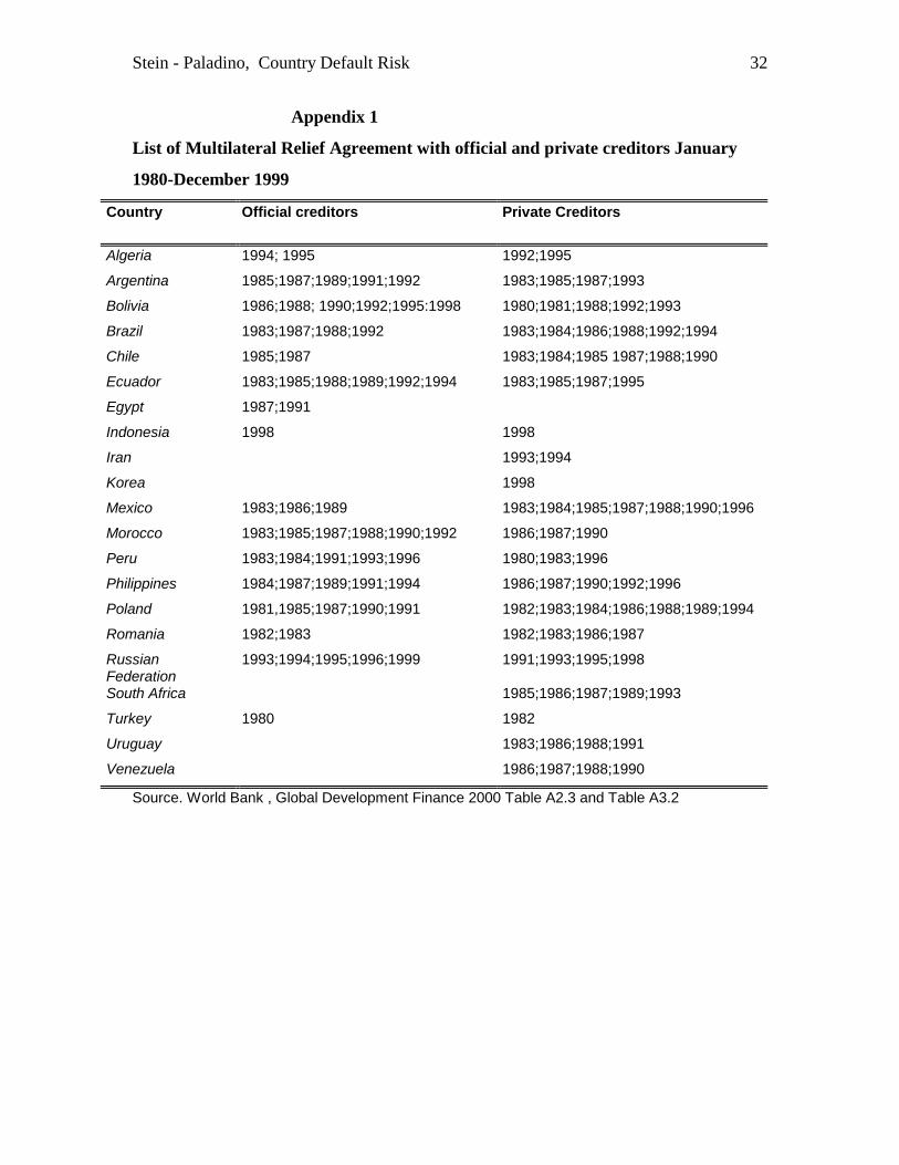
creditors during the period January 1980 - December 1999. Appendix 1 and table A2,

derived from the World Bank "Global Development Finance", list the entire set of

countries that rescheduled and the dates of agreement. These countries are contrasted

with thirteen emerging market countries that did not default, table A3.

The basic variables are10: the actual external public debt/GDP ratio h(t), the

productivity of capital b(t), the interest rate r(t) on foreign currency denominated debt, the

growth rate g(t) of real GDP, and the ratio j(t) of investment/GDP. An estimate of the

gross productivity of capital b(t) is the inverse ICOR11, where b(t) = dY(t)/dK(t) =

[dY(t)/dt /Y(t)] / [J(t)/Y(t)] = g(t)/j(t), equal to the growth rate of GDP divided by the ratio

9 In some cases, private borrowing was supported by implicit government guarantees.10 Our data are from: World Bank (Global Development Finance), the IMF(International Financial Statistics) and IIF( countries data sets).11 ICOR is the incremental capital output ratio.


of gross investment/GDP. The net return x(t) = b(t) - r(t). The productivity of investment

b(t) is gross of depreciation and obsolescence.

The debt/GDP ratio combines short and long term external debt, but the

theoretical analysis is based upon a two period model where the debt plus interest must be

repaid. A similar relation between the optimal debt/GDP and the net return is found in

both the infinite horizon model and in the two period model. The difference is that in the

two period model, the debt plus interest must be repaid by the end of period two; and in

the infinite horizon model, the only requirement is that the debt must always be serviced.

Operationally, the only significant difference is in the concept of the maximal debt f-max.

Given the mix of maturities, we use the inclusive measure of the external debt.

The application of the Fleming-Stein theoretical analysis is carried out in two

parts. First: we compare Mexico, a country that defaulted/rescheduled his debt, with

Tunisia which did not default. Second: we examine the panel data of the countries that

defaulted relative to those that did not.

3.1. Comparison between Mexico and Tunisia

Mexico experienced currency crises in September 1976, February and December

1982 and December 1994, and concluded ten debtrescheduling agreements with

commercial banks, and three with official creditors, during the two decades January 1980

- December 1999 (see appendix 1). These agreements were concentrated in the periods

1983-90 and 1996. Tunisia is not listed among the countries that rescheduled. A

comparison of the two countries provides us a better understanding of the subsequent

panel data analysis. Table 1 summarizes the basic relations used in our analysis.

Table 1. COMPARISON OF MEXICO AND TUNISIA

The median debt/GDP, row 1, was higher in Tunisia (0.61), which did not default

than in Mexico (0.45), which rescheduled many times in our sample period 1980-99. It is

not the debt ratio h(t) that determines the probability of default, but rather an excess of the

actual ratio h(t) compared to the debt-max.


Equation (10), repeated here, is the relation between the debt and j(1) which will

lead to a zero consumption in the bad case, when b(2) = b-(2). This corresponds to the

situation in figure 1. When c(1) is on or above the triangle 0AB, then default will occur in

the bad case. The f-max corresponds to the hypotenuse line AB, as described in section

2.3.1 above. The value of f-max in (10) is conditional upon the rate of investment j(1).

We see in table 1, row 5, that there was a small variance to the rate of investment/GDP in

the countries. We use the median rate of investment as j(1). The interest rate is in row 4.

Box 1 above presents our theoretical concept of the distribution of the gross return

b(2) in the good and bad cases. Figures 3 and 4 are histograms of the gross return b(t)

denoted B1 in Mexico which defaulted/rescheduled and Tunisia which did not,

respectively. It is essential to study these histograms to estimate b(2) in the good and bad

cases.

In the Mexican case, the left tail of the gross return b(t) figure 3, reflects the debt

crises periods 1994-95, where the return fell drastically as a consequence of the crisis. We

minimize the weight of these outliers in the distribution of b (t) the gross return, by taking

as our measure of the expected return E[b(2)] = 0.15 in row 2 to be the median gross

return. We assume that b(1) was equal to the expected return The distribution of b(t) is

stationary/mean-reverting. The standard deviation of the gross return 0.16 is taken to be

an estimate of (a/2). Therefore the bad case b-(2) = .15 - .16 = -0.01, in row 3. The

investment ratio j(1) is the median investment/GDP ratio 0.22, in row 5; and the interest

rate r is taken as the median 0.08 in row 4.

The f-max for Mexico, based upon (10) is (10-MEX) equal to the maximal

debt/GDP that Mexico can have and yet repay if the bad event occurs. It is based upon the

histogram in figure 3 and data in table 1. Row 8, column 1 in table 1, states that f-max for

Mexico is 0.13. A similar calculation for Tunisia implies that f-max is 0.73: row 8,

column 2, in table 1 above.

f-max = [(b-(2)/b(1)) + (1 + b-(2))j(1)] / (1 + r) (10)

f-max = [(-0.12)/(.15) + (1 - .012)(.22)] / (1.08) = .13 (10-MEX)

It is not the debt ratio h(t) that is relevant for default (DEF), but the excess of the

actual debt over f-max. We calculate the difference (DEF) between the actual median

debt and f-max. If DEF > 0, then the debt is “excessive” and the country is likely to


default in the event that the bad case occurs. The resulting values of DEF = [actual

median debt/GDP - (f-max)] is in the row 9 of table 1. In Mexico, DEF = .45 - .13 = .32

and in Tunisia, DEF = -.116. Since the Mexican debt exceeded f-max, then default would

occur if the bad event arose.

Figure 5 is even more revealing. We plot the annual DEF(t) = h(t) - (f-max) =

actual debt/GDP in each year less the f-max (row 9 in table 1), for Mexico and Tunisia. In

Mexico, there was an excess debt DEF > 0 in every year 1978-99. In Tunisia, the excess

debt DEF < 0, except for a short period when it was slightly positive. The conclusions are

Mexico would default/reschedule, whereas Tunisia could repay the debt.

Figure 3. Mexico. Histogram of gross return b(t) = growth/investment ratio

Figure 4. Tunisia. Histogram of gross return b(t) =growth/investment ratio

Figure 5: Excess debt = DEF = debt/GDP - (debt/GDP)max, in Mexico and Tunisia


0

2

4

6

8

-40 -30 -20 -10 0 10 20 30 40

Series: B1_MEXSample 1981 1999Observations 19

Mean 10.19493Median 15.12098Maximum 30.97354Minimum -31.11466Std. Dev. 16.27297Skewness -1.193285Kurtosis 3.450504

Jarque-Bera 4.669781Probability 0.096821

Figure 3Mexico Histogram of rate of return B1 = b(t)= growth rate/investment ratio


0

1

2

3

4

5

-0.1 0.0 0.1 0.2 0.3

Series: B1_TUSample 1979 1998Observations 20

Mean 0.153383Median 0.166540Maximum 0.271218Minimum -0.081165Std. Dev. 0.093626Skewness -0.833685Kurtosis 3.102572

Jarque-Bera 2.325536Probability 0.312620

Figure 4.

Tunisia. Histogram of rate of return B1 = b(t).


-0.4

-0.2

0.0

0.2

0.4

0.6

0.8

78 80 82 84 86 88 90 92 94 96 98

DEF_MEX DEF_TUFigure 5MEXico, TUnisiaExcess debt/GDP, DEF(t) = (debt/GDP)(t) - (f-max),


Table ICOMPARISON OF MEXICO AND TUNISIA

Variable: median, [range], (σ) MEXICO ADF TUNISIA ADF

1.Debt/gdp = h(t) .45 [.81, .29](.14) -2.5 .61 [.74, .44](.09) -1.8

2.Gross return = b(t) .15 [.30, -.31](.16) -3.3* .167[.27,-.08] (.09) -3.5*

3. bad case b-(2) (median b(2)- 1σ) =-.012

(median b(2)-1σ) =.077

4.Interest rate= r(t) .08 [.15, .07] (.02) -1.89 .05[.06,.04] (.004) -3.67*

5.Investment/gdp = j(t) .22 (.02) -1.55 .28 (.04) -3.67*

6.Net return= x(t) .057[.17,- .39](.16) -2.1 .107 [.21,-.13](.09) -3.47*

7.Growth = g(t) .035[.08,-.06] (.036) -3.07* .049[.086, -.02] (.028) -3.5*

8.f-max .13 .73

9.DEF = h(t) - f-max .322 -.116

10.Cor(h,x) -.67 -.24

11.Cor(b,r) .02 -.11

Actual debt/GDP = h(t); maximal debt/GDP = f-max. We use median b(1), j(1), r(1) to eliminate the outlierwhich may have been the consequence of the currency crisis. ADF is significant if there is an asterisk. f-max = [b-(2)/b(1) + (1+b-(2)) j(1)]/(1+r) is evaluated at the median investment ratio j(t). The net return is:x(t) = b(t) - r(t).


3.2. Panel data analysis

The theory figure 2 describes the relation between f*(t) the constrained optimal

debt/GDP and the expected net return E[x(t)]. The net return x(t) = b(t) - r(t) = g(t)/j(t) -

r(t), where g(t) is the growth rate and j(t) is the investment ratio. As x(t) varies around a

stationary mean E[x(t)], the optimal f(t) should be constant. If one simply compared the

actual net return x(t) = g(t)/j(t) - r(t) with the actual debt/GDP , there is a negative bias.

When a crisis occurs, the growth rate g(t) declines and the actual GDP may fall. This

tends to raise h(t) = L(t)/Y(t) and lower the net return x(t). A noteworthy example is

Mexico (default), during the crisis 1980-82. The drastic decline in the return and the rise

in the debt/GDP may have been consequences of the crisis and reactions to it. An analysis

of panel data: country by sub-period may diminish the effect of the bias between

debt/GDP and net return.

Appendix tables A2 and A3 contain the panel data for the two sets of countries:

default/reschedule and a control group that did not default. The default countries are:

Algeria, Argentina, Bolivia, Brazil, Chile, Ecuador, Egypt, Honduras, Indonesia, Iran,

Korea, Mexico, Morocco, Peru, Philippines, Poland, Romania, Russia, South Africa,

Turkey, Uruguay, Venezuela. The control countries are: China, Czech Republic, Estonia,

Hungary, Slovenia; India, Kuwait, Lebanon, Malaysia, Saudi Arabia, Tunisia, United

Arab Emirates, Zimbabwe. The growth and stability in the control set of countries are

tenuous, investment there is very risky, but they have not as yet defaulted. Tables A2 and

A3 contain the values of debt/GDP = h(t), the return = b(t), the interest rate r(t), the net

return x(t) = b(t) - r(t), and the investment/GDP ratio = j(t), during four periods: 1980-84,

1985-89, 1990-94, 1995-99. Table 2 summarizes the key relations that are pertinent to our

analysis.

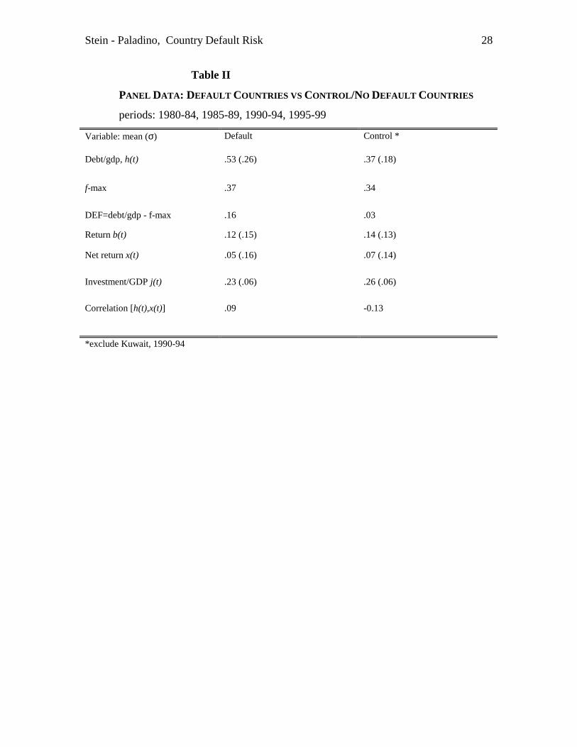
Table II


Scatter diagram figure 6 relates the h(t) = debt/GDP ratio to the x(t) = net return in a

panel of default/reschedule countries. Figure 7 does the same for the countries that did not

default/reschedule.

Figure 6. Scatter diagram, panel data Default countries: debt/GDP on net return

Figure 7. Scatter diagram, panel data Control countries: debt/GDP on net return


0.0

0.5

1.0

1.5

2.0

-0.6 -0.4 -0.2 0.0 0.2 0.4 0.6

DEB

T

NETRETURN

Figure 6. Default/reschedule countriespanel: 1980-84, 1985-89,1990-94,1995-99h(t) = debt/GDP on x(t) = net return


0.0

0.2

0.4

0.6

0.8

1.0

-0.5 0.0 0.5 1.0 1.5

DBT

GD

P

NETRETURNFigure 7Control group panel: 1980-84, 1985-89,1990-94,1995-99h(t) = debt/GDP on x(t) = net return


Our conclusions are the following, based upon scatter diagrams figures 5,6,7 and

table 2. (A) In neither set of countries was the debt-net return relation even qualitatively

optimal. Both sets of countries are poor credit risks indeed. (A1) In neither set of

countries is the debt/GDP ratio positively and significantly correlated with the net return

(A2) Positive debt is associated with a zero net return, despite the great risk measured by

the standard deviation of the return. Compare figures 6-7 with the constrained optimal

case figure 2, where a positive debt is only optimal if the expected net return exceeds a

quantity d > 0, where d is positively related to the downside risk. (B) Both sets of

countries were similar except in one respect. Table 2 shows that: (B1) The median net

return x was higher, but not significantly so, in the control group. (B2) The investment

ratios j(t) were similar. (B3) The maximal debt/GDP was similar in the two groups. The

crucial difference was that: (C1) the actual debt/GDP was significantly higher in the

default group. (C2) Since the value of f-max was similar, the DEF = excess debt/GDP

was significantly positive 0.16 among the default countries, whereas DEF was not

significantly positive among the control countries.


Table II

PANEL DATA: DEFAULT COUNTRIES VS CONTROL/NO DEFAULT COUNTRIES

periods: 1980-84, 1985-89, 1990-94, 1995-99

Variable: mean (σ) Default Control *

Debt/gdp, h(t) .53 (.26) .37 (.18)

f-max .37 .34

DEF=debt/gdp - f-max .16 .03

Return b(t) .12 (.15) .14 (.13)

Net return x(t) .05 (.16) .07 (.14)

Investment/GDP j(t) .23 (.06) .26 (.06)

Correlation [h(t),x(t)] .09 -0.13

*exclude Kuwait, 1990-94


3.3 Early Warning Signals (EWS) of bubbles, vulnerability to shocks and default

We can derive early warning signals that an economy is vulnerable to shocks that

will lead to a default/rescheduling. Based upon the evidence in tables 1 and 2, the EWS of

the rescheduling should be a DEF(default) variable that is significantly positive and

persistent. To avoid false signals we require that, to be taken as an on-signal, DEF = [h(t)

- (f-max)] = [debt/GDP - (debt max /GDP)] be positive and either exceed one standard

deviation or that it has been rising. To examine the explanatory power of such a system

we construct a 2X2 contingency table 3. Each country in each sub-period is considered

one observation. The default (control) country data are in appendix table A2 (A3).

The rows of table 3 are the signal on/off. The first row refers to the on-signal. It is

conditioned on (a) the sign of DEF and whether either (b1) or (b2) below is satisfied. The

second row is the off- signal: the complement of the first row.

On-signal

(a) DEF= [h(t) - (f-max)] > 0, and one of the following:(b1) DEF > 1σ or (b2) DEF rising.

The columns in table 3 refer to the occurrence/non-occurrence of rescheduling during the

subperiod. Rescheduling is a legal act and comes after a period of difficulties. A caveat is

that political factors are operating so that there is often a political bailout. However, if the

country falls in row 1, this may be an EWS of a political bailout.

Table III, Contingency table by country

In 84% ( = 43/51) of the periods of rescheduling the DEF variable has been

positive and was either greater than 1 standard deviation or rising. In contingency table 3,

each country has been analysed by sub-period. The rows refer to the on/off signal. The

columns refer to the occurrence/non-occurence of rescheduling during the subperiod.

The χ2 test concerns the independence of the rows and columns. Since the value of χ2(1)


= 17.6 falls in the rejection region, we have to reject the null hypothesis of independence

of the two classification12.

The conclusion is that: In the event of the bad case the countries in row 1, those

who have large and positive DEF, are expected to default, whereas those in row 2 where

DEF < 0 are not. Applying the Fleming/Stein mathematical analysis, we have provided

quantitative measures of whether economies are vulnerable to shocks that may lead to

default. These measures have been shown to have significant explanatory value.

12 To further investigate the explicative power of the DEF= [h(t) - (f-max)] variable, we carried out a probitanalysis. The results are encouraging. The DEF is significant and positive, with a marginal effect of 11%.


Table IIICONTINGENCY TABLE BY COUNTRY

Number of observation in that category (expected cell frequency);Total Number of obs. 127

Recheduling No Rescheduling Total

DEF>0; and(i)DEF >1 σor (ii) DEF rising

43(30.8) 36(46.2) 79

DEF<0and(i)DEF<1 σor (ii) DEFdeclining

8(19.2) 40(28.8) 48

Totals

χ2 = 17.6 (1 d.f)**

51 76 127

Note: Each country has been analysed by sub-period, based upon appendixes 2 and 3.


Appendix 1

List of Multilateral Relief Agreement with official and private creditors January

1980-December 1999

Country Official creditors Private Creditors

Algeria 1994; 1995 1992;1995

Argentina 1985;1987;1989;1991;1992 1983;1985;1987;1993

Bolivia 1986;1988; 1990;1992;1995:1998 1980;1981;1988;1992;1993

Brazil 1983;1987;1988;1992 1983;1984;1986;1988;1992;1994

Chile 1985;1987 1983;1984;1985 1987;1988;1990

Ecuador 1983;1985;1988;1989;1992;1994 1983;1985;1987;1995

Egypt 1987;1991

Indonesia 1998 1998

Iran 1993;1994

Korea 1998

Mexico 1983;1986;1989 1983;1984;1985;1987;1988;1990;1996

Morocco 1983;1985;1987;1988;1990;1992 1986;1987;1990

Peru 1983;1984;1991;1993;1996 1980;1983;1996

Philippines 1984;1987;1989;1991;1994 1986;1987;1990;1992;1996

Poland 1981,1985;1987;1990;1991 1982;1983;1984;1986;1988;1989;1994

Romania 1982;1983 1982;1983;1986;1987

RussianFederation

1993;1994;1995;1996;1999 1991;1993;1995;1998

South Africa 1985;1986;1987;1989;1993

Turkey 1980 1982

Uruguay 1983;1986;1988;1991

Venezuela 1986;1987;1988;1990

Source. World Bank , Global Development Finance 2000 Table A2.3 and Table A3.2


Appendix 2

Table A2

Summary Table Default Group

1980-1984 1985-1989 1990-1994 1995-1999

Country b(t) Rn(t) j(t) h(t) b(t) rn(t) j(t) h(t) b(t) rn(t) j(t) h(t) b(t) rn(t) j(t) h(t)

Algeria (ALG) 0.117 0.085 0.370 0.394 0.056 0.072 0.309 0.421 -0.012 0.070 0.278 0.611 0.148 0.065 0.241 0.722

Argentina (AR) 0.013 0.106 0.201 0.373 -0.073 0.082 0.125 0.640 0.333 0.064 0.176 0.369 0.117 0.069 0.188 0.446

Bolivia (BOL) -0.053 0.114 0.142 0.594 0.089 0.063 0.146 0.996 0.277 0.049 0.151 0.826 0.212 0.050 0.190 0.694

Brazil (BR) 0.683 0.122 0.169 0.369 0.225 0.087 0.223 0.396 0.079 0.058 0.215 0.348 0.098 0.062 0.217 0.317

Chile (CHL) 0.082 0.127 0.156 0.696 0.289 0.093 0.212 0.968 0.303 0.077 0.244 0.486 0.206 0.054 0.255 0.410

Ecuador (ECU) 0.097 0.110 0.218 0.508 0.125 0.085 0.207 0.917 0.178 0.056 0.201 1.015 -0.034 0.059 0.185 0.879

Egypt (EGY) 0.334 0.052 0.302 0.904 0.184 0.054 0.298 1.521 0.154 0.049 0.226 0.885 0.262 0.034 0.208 0.408

Indonesia (INDO) 0.249 0.084 0.258 0.200 0.160 0.066 0.325 0.599 0.229 0.056 0.335 0.601 -0.008 0.057 0.248 0.883

Iran (IR) 0.331 0.030 0.201 0.070 -0.097 0.013 0.145 0.022 0.354 0.008 0.199 0.207 0.093 0.052 0.229 0.195

Korea (KOR) 0.213 0.099 0.304 0.510 0.307 0.072 0.311 0.383 0.203 0.049 0.371 0.208 0.125 0.046 0.320 0.341

Mexico (MEX) 0.061 0.135 0.226 0.448 0.062 0.086 0.205 0.628 0.174 0.079 0.220 0.384 0.101 0.079 0.237 0.446

Morocco (MOR) 0.152 0.050 0.253 0.840 0.214 0.045 0.231 1.02 0.146 0.056 0.228 0.768 0.097 0.058 0.212 0.592

Peru (PER) 0.012 0.098 0.282 0.472 0.010 0.072 0.281 0.601 0.157 0.057 0.180 0.665 0.171 0.058 0.234 0.521

Philippines (PHIL) -0.018 0.074 0.268 0.656 0.176 0.063 0.170 0.839 0.077 0.056 0.286 0.606 0.161 0.047 0.220 0.671

Poland (POL) -0.112 0.117 0.247 0.383 0.105 0.086 0.314 0.514 -0.025 0.057 0.187 0.619 0.259 0.048 0.222 0.362

Romania (ROM) 0.111 0.095 0.356 0.228 -0.023 0.078 0.308 0.093 -0.143 0.039 0.286 0.127 -0.061 0.051 0.219 0.240

Russian Fed (RUS) na na na na na na na na -0.390 0.065 0.236 0.401 -0.104 0.072 0.189 0.515

South Africa (SAF) 0.100 0.105 0.267 0.266 0.077 0.087 0.191 0.325 0.012 0.077 0.153 0.213 0.141 0.075 0.161 0.267

Turkey (TUR) 0.207 0.085 0.264 0.331 0.257 0.070 0.231 0.482 0.140 0.063 0.241 0.376 0.164 0.056 0.239 0.494

Uruguay (URU) -0.141 0.081 0.146 0.562 0.317 0.075 0.122 0.889 0.299 0.062 0.137 0.672 0.134 0.058 0.155 0.637

Venezuela (VEN) -0.124 0.133 0.206 0.586 0.020 0.100 0.211 0.651 0.249 0.081 0.169 0.661 0.132 0.075 0.184 0.431


Table A3

Summary Table Control Group

1980-84 1985-89 1990-94 1995-99

Country + x(t) rn(t) j(t) h(t) x(t) rn(t) j(t) h(t) x(t) rn(t) j(t) h(t) x(t) rn(t) j(t) h(t)

China (CI) na 0.11 na 0.03 0.21 0.03 0.36 0.12 0.22 0.05 0.38 0.18 0.17 0.04 0.39 0.18

Cezch Republic (CK) na na na na 0.04 0.10 0.27 0.14 -0.16 0.08 0.25 0.24 -0.03 0.08 0.32 0.39

Estonia (ESTO) na na na na na na na na -0.12 0.03 0.26 0.15 0.10 0.05 0.27 0.45

Hunghary (HUNG) -0.03 0.10 0.28 0.49 -0.03 0.08 0.27 0.70 -0.23 0.07 0.21 0.64 0.03 0.08 0.28 0.58

India (IN) 0.21 0.02 0.24 0.15 0.20 0.03 0.25 0.24 0.14 0.05 0.24 0.32 0.20 0.06 0.25 0.26

Kuwait (KW) -0.10 0.10 0.16 0.47 0.47 0.07 0.13 0.43 1.28 0.06 0.17 0.87 -0.08 0.08 0.12 0.58

Lebanon (LB) na na na na na na na na 0.25 0.06 0.27 0.34 0.01 0.10 0.36 0.37

Malaysia (MAL) 0.11 0.07 0.36 0.46 0.10 0.07 0.28 0.71 0.37 0.06 0.38 0.50 0.05 0.06 0.37 0.45

Saudi Arabia (SARA) -0.12 0.12 0.25 0.14 0.01 0.07 0.19 0.20 0.13 0.07 0.21 0.16 -0.01 0.08 0.19 0.20

Slovenia (SLO) na na na na na na na na -0.21 0.09 0.18 0.32 0.11 0.05 0.24 0.36

Tunisia (TU) 0.10 0.06 0.33 0.48 0.04 0.05 0.24 0.48 0.11 0.05 0.28 0.60 0.13 0.05 0.27 0.63

United ArabEmirates

(UAE) -0.09 0.14 0.28 0.22 0.02 0.08 0.24 0.36 0.15 0.06 0.25 0.45 0.08 0.05 0.27 0.46

Zimbawe (ZW) 0.16 0.08 0.2 0.27 0.18 0.07 0.17 0.03 0.05 0.06 0.21 0.53 0.08 0.04 0.22 0.69


REFERENCES

Alba, Pedro et al. (1999), "The Role of macroeconomics and financial sector linkages inEast Asia's financial crisis", in Pierre-Richard Agénor, Marcus Miller, David Vines andAxel Weber, (ed.), The Asian Financial Crisis, Cambridge University Press.

Corbett, J.and D. Vines (1999), "The Asian crisis: lessons from the collapse of financialsystems, exchange rates and macroeconomic policy", in Pierre-Richard Agénor, MarcusMiller, David Vines and Axel Weber, (ed.), The Asian Financial Crisis, CambridgeUniversity Press.

Corsetti, G., P. Pesenti and N. Roubini, (1999), "The Asian Crisis: an overview of theempirical evidence and policy debate", in Pierre-Richard Agénor, Marcus Miller, DavidVines and Axel Weber, (ed.), The Asian Financial Crisis, Cambridge University Press.

Fleming, Wendell H. and Jerome L. Stein (1999), “A Stochastic Optimal ControlApproach to International Finance and Foreign Debt”, CESifo Working Paper # 204,available at http://www/CESifo.de

Fleming, Wendell H. and Jerome L. Stein (2001), “Stochastic Inter-temporalOptimization in Discrete Time”, in Negishi, T., Rama Ramachandran and Kazuo Mino(ed.), Economic Theory, Dynamics and Markets: Essays in Honor of Ryuzo Sato, Kluwer.An earlier version is available as CESifo Working Paper #338, available athttp://www/CESifo.de

Infante, Ettore and Jerome L. Stein (1973),”Optimal Growth with Robust FeedbackControl”, Review Economic Studies, XL(1)

International Monetary Fund, (1999) ,International Capital Markets, Washington DC

International Monetary Fund, (1999).Anticipating Balance of Payments Crises,Occasional Paper #186,

Stein, Jerome L. and Giovanna Paladino (1997) “Recent Developments in InternationalFinance: A Guide to Research”, Journal of Banking and Finance 21 (11-12).

Country Default Risk: An Empirical Assessment

Documents

Transcript of Country Default Risk: An Empirical Assessment