Balance sheet effects and the country risk premium: an empirical investigation

DOCUMENTO DE TRABAJO

BALANCE SHEETEFFECTS AND THE

COUNTRY RISKPREMIUM:

AN EMPIRICALINVESTIGATION

Documento de Trabajo n.º 0316

BANCO DE ESPAÑA

SERVICIO DE ESTUDIOS

and Alicia García HerreroJuan Carlos Berganza, Roberto Chang

BALANCE SHEET EFFECTS AND THE

COUNTRY RISK PREMIUM:

AN EMPIRICAL INVESTIGATION (1)

Documento de Trabajo nº 0316

Juan Carlos Berganza (2), Roberto Chang (3)

and Alicia García Herrero (4) (1) We would like to thank Raquel Carrasco for her valuable suggestions and Lucía Cuadro for her excellent research assistance. W e are also grateful for comments from Guillermo Le Fort, Klaus Schmidt -Hebbel, Ugo Panizza, Javier Valles, an anonymous referee, and participants to seminars in the Kiel Institute of World Economics, Banco de España, and the Euro-Latin IADB network on regional integration. Remaining errors are only ours. Finally, the opinions expressed are those of the authors’ and do not necessarily reflect those of the Banco de España. (2) Banco de España ([email protected]) (3) Rutgers University.( [email protected]). Much of Chang’s work for this project was completed while a visiting scholar at Banco de España, whose hospitality he acknowledges with gratitude. He also thanks the National Science Foundation for financial support. (4) Banco de España ( alicia.garcia [email protected])

BANCO DE ESPAÑA SERVICIO DE ESTUDIOS

The Working Paper Series seeks to disseminate original research in economics and finance. All papers have been anonymously refereed. By publishing these papers, the Banco de España

aims to contribute to economic analysis and, in particular, to knowledge of the Spanish economy and its international environment.

The opinions and analyses in the Working Paper Series are the responsibility of the authors and,

therefore, do not necessarily coincide with those of the Banco de España or the Eurosystem.

The Banco de España disseminates its main reports and most of its publications via the INTERNET at the following

website: http://www.bde.es

Reproduction for educational and non-commercial purposes is permitted provided that the source is acknowledged

© BANCO DE ESPAÑA, Madrid, 2003 ISSN: 0213-2710 (print)

ISSN: 1579-8666 (online) Depósito legal: M. 55150-2003Imprenta del Banco de España

Abstract

This paper investigates empirically whether there is a negative relationship between a country’s

risk premium and the balance sheet effect, as implied by recent theories emphasizing financial

imperfections. We find evidence that balance sheet effects, stemming from the increase in the

external debt service after an unexpected real depreciation, significantly raise the risk premium.

We also show that the increase in the risk premium is not due to the debt service as such. While

the result holds for the whole sample, we show that it is mainly driven by those countries with the

largest financial imperfections, as argued by imperfect capital market theories. Particularly large

real depreciations also seem to be disproportionately important, meaning that the balance sheet

effects may be strongest at times of economic crisis, when large devaluations occur.

JEL Classification: F3, F31, F34

Key words: balance sheet effects, country risk premium, sovereign spreads

7

1. INTRODUCTION

Conventional open economy models, and in particular the influential Mundell-Fleming model,

imply that a real devaluation switches demand towards domestic production and is expansionary.

But recent theories on credit constraints and balance sheet effects have challenged this view. The

argument starts with the observation that if a country has a large debt with the rest of the world,

and the value of the debt depends on the real exchange rate, a devaluation causes a fall in the

country’s net worth. In the presence of financial imperfections, the balance sheet effect of a

devaluation implies an increase in the cost of credit, a fall in aggregate demand, and hence a

contraction in economic activity5. This mechanism may be particularly strong in emerging

countries since these countries generally borrow in foreign currency and are subject to sharp real

exchange rate depreciations (or devaluations).

Recent theoretical studies have developed the above argument in some detail; noteworthy

contributions include Aghion, Bacchetta and Banerjee (2001), and Céspedes, Chang and

Velasco (2000). The empirical evidence is, however, scarce at this point, although sorely needed

since the theory by itself cannot determine whether the balance sheet effect of a devaluation is

strong enough to reverse conventional wisdom.

This paper is an attempt to investigate the issue empirically. Our approach is to test whether

balance sheet effects that emerge when the value of the external debt burden changes due to a

real exchange depreciation significantly increase country risk in emerging countries. An

affirmative answer is supported by our evidence.

For a panel of emerging economies in the last decade, we construct a “balance sheet” variable by

computing the change in the value of the debt service associated with unanticipated real

depreciations. We find that this variable is significant in explaining the variation of the cost of

credit in those economies. We argue that our findings are not due to the effect of the amount of

debt owed, and that the impact of the balance sheet effects of a real depreciation are stronger

during economic crises and in countries with higher degrees of financial imperfections. These

results should obviously be corroborated by further work, but seem highly stimulating and

relevant to current debates.

5 Country risk excludes the changes that might occur in US interest rates, which are obviously exogenous. The external cost of credit includes both.

8

The only paper that attempts an empirical exercise similar to ours is Bleakley and Cowan (2002)

but it differs from ours in substantial ways. Bleakley and Cowan investigated a panel of firms

from Latin America countries, and hence focused on micro data, as opposed to our work which is

based on macro data. Bleakley and Cowan focused on investment, not the cost of credit. And,

finally, their results are quite different: they found that firms with a larger amount of debt in

dollar tend to invest more after a real depreciation, which runs contrary to the implications of the

recent literature on credit constraints although the authors do not control for the degree of

constraints for each firm. Our results, in turn, are much more supportive of that literature.

Section 2 offers a simple theoretical framework for our empirical test. Section 3 describes the

data used and the empirical challenges. Section 4 offers the findings. Finally, Section 5 draws

some preliminary conclusions and points to venues of future research.

2. THEORETICAL AND EMPIRICAL FRAMEWORK

This section illustrates with a very simple theoretical framework the implications of recent

theories on the interaction between balance sheet effects, dollarized liabilities, and exchange rates

that justify our empirical focus. Consider a small open economy, indexed by i , whose residents

borrow in the international capital markets. One may assume that the borrowing amount is fixed

in terms of an international currency (henceforth called dollar). We denote by it the spread

between the interest rate charged to that borrower and the world interest rate, or risk premium for

short. The key question we address is whether there is an inverse relation between the risk

premium and the value of the borrower´s own funds available for investment:

)(1 itit (1)

where is a strictly decreasing function and it denotes real net worth, that is, net worth

measured in terms of the country´s final (consumption or investment) goods. Final goods are

assumed to be a composite of tradables and nontradables.

Equation (1) is the hallmark of recent theories of balance sheet effects and financial

imperfections and can be justified in at least two different but related ways. The first one,

associated with the work of Cespedes, Chang and Velasco (2000), and Gertler, Gilchrist and

Natalucci (2001), and others, stresses the effects of a devaluation on the financial agency costs

9

due to asymmetric information or imperfect enforcement: the smaller a borrower´s net worth, the

more he or she needs to rely on external finance, which increases agency costs. Since the

international capital market is assumed to be competitive and foreign lenders base their decisions

on their opportunity cost of funds, higher expected agency costs raise the risk premium. A

slightly different view, associated with Hart and Moore (1994) and Kiyotaki and Moore (1997),

is that the costs of borrowing decrease in the value of the collateral that the borrower can post

against the loan. If collateral is given by the real value of the borrower´s net assets, (1) follows.

Recent international macro models take the above formulation as a starting point, and add the

observation that international debt obligations are very often “dollarized”, that is, denominated in

foreign currency. Under such circumstances, which are typical of emerging economies, a real

exchange depreciation can easily reduce the dollar value of domestic net worth so that, under (1),

the cost of credit must increase relative to the world interest rate (i.e., the country risk must rise).

To see how that implication is derived, let us assume that the net worth can be expressed as

itititit XDZ (2)

where itD is the country´s debt, in dollars, due in period t , itX is the real exchange rate (the

price of dollars in terms of the country´s final good), and itZ denotes other determinants of net

worth in period t . Let i and i denote the mean values of it and it . Then, taking a linear

approximation to (1) around i ,

)()(1 iitiit

it

ititit XDZ (3)

where ' denotes the negative of the first derivative of evaluated at i , is a

constant, and the last equality follows from (2).

The value of is of particular interest, as it is crucial for the recent debate on the implications

of a real exchange depreciation. If country i has a substantial debt burden in dollar, a real

depreciation (an increase in itX ) will make i's net worth fall, ceteris paribus. Then, if is

10

significantly positive, the risk premium it must increase. This reasoning, however, is based on

the crucial assumption of a positive . In reality, these theories do not necessarily predict

that should be different from zero: in the absence of financial imperfections, there should be

no connection between the cost of credit and i’s net worth, and should be zero. In turn,

should be larger than zero if there are financial imperfections. Our empirical work will,

therefore, focus on testing whether is significantly positive and in which circumstances, in

terms of financial imperfections. This requires further elaboration of the basic relationship (3).

The immediate empirical problem is that the net worth is not directly observable: while it

depends on the external debt burden, it may also depend on other variables, such as the amount of

current resources available to reduce the need for external finance. In practice, these other

variables (which we have collapsed into the variable itZ ) are very difficult to observe. So we

proceed in a slightly different direction.

A convenient assumption to reach a testable equation is that itD is predetermined as of period t .

Then, taking the expectation of (3) conditional on information available at 1t , and subtracting

the result from (3), we get:

itittititittit XEXDE )( 11 (4)

where )(1tE denotes the conditional expectation operator, and )( 1 lttltit ZEZ is the

unexpected component of itZ .

Equation (4) simply decomposes the unexpected change in i's country risk into two components. The

first is the impact of an unanticipated increase in the external debt burden, given by a linear

function of the debt burden times the unexpected real depreciation. The second component is the

effect of unanticipated changes in other components of net worth. If we treated the latter as an

unobservable shock, we could estimate equation (4) provided that it is uncorrelated

with )( 1 ittitit XEXD . Since itD is assumed to be predetermined, the latter condition would

imply that it be uncorrelated with ittit XEX 1 . As a first step, we assume this to be the case,

11

but we will test for omitted variables in the empirical part. There, we shall also relax the

assumption that the debt burden is predetermined.

To implement equation (4) econometrically, we resort to two further approximations. First, we

replace the expectation of the country risk in t-1, it1-tE , with a linear function of predetermined

variables, 1,tiiY (where 1,tiY and i are conformable vectors). Second, we replace the term

itt XE 1 with 1,tiX ; this is likely to entail little loss, since real exchange rates are usually very

close to random walks, at least in the case of pure floats or fixed exchange regimes6. In the case

of intermediate regimes, the lack of hedging opportunities in many emerging countries could

make this assumption less restrictive than thought at first sight.

The resulting equation to estimate is:

ittiitit YS 1, (5)

where )( 1*

itititit XXDS is interpreted as the change in the value of country’s i’s external

debt burden due to an unanticipated real exchange depreciation in period t. As already mentioned,

our key concern is whether the impact of the balance sheet effects on the cost of credit, the

coefficient , is significantly positive and whether this depends on the degree of financial

imperfections.

3. THE DATA

The empirical implementation of equation (5) involves several data difficulties, the main one

being related to measuring the risk premium variable ( it). That variable represents, in theory, the

cost of credit on the marginal funding for country i during year t. In practice, unfortunately,

available measures of the cost of credit seem very far from that ideal. The best available proxy,

and the most widely used in the literature, are the returns implicit in the Emerging Markets Bonds

Indices (EMBI), provided by JP Morgan. For each country and year in that dataset we construct a

credit spread measure (COSTBORROWING) by subtracting total returns on US Treasury bonds

from that country’s EMBI returns. We limited our sample to countries with at least four

observations of EMBI returns, which reduces the sample to twenty-seven countries. Ten of them

6 The exception would be crawling pegs.

12

have data from 1993, when the EMBI started being produced and all countries have data for the

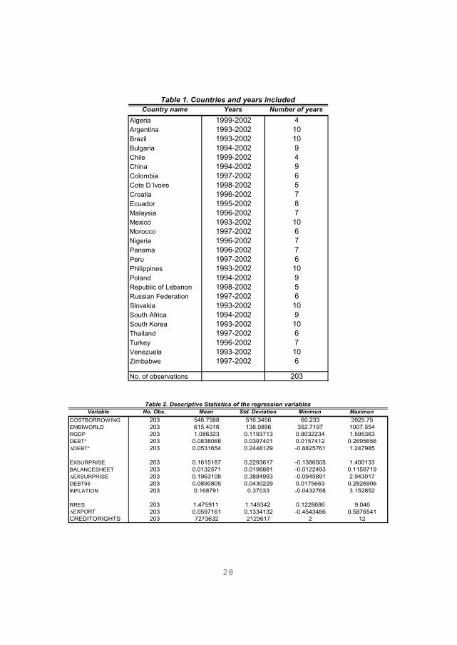
last year, 2002. Given this data constraints, the total sample is composed of 203 yearly

observations. Table 1 in Appendix 1 lists the countries and the data availability while Appendix 2

offers a detailed description of the variable definitions and sources.

To proxy for the balance sheet term itS in equation (5), we construct a variable called

BALANCESHEET, which is an interaction term, namely the product of EXSURPRISE and

DEBT*. EXSURPRISE equals the change in i’s real exchange rate (EX as defined in

Appendix 2) between year t and year t-1, and DEBT* is the US dollar value of i’s debt service

due in year t divided by i’s GDP in 1995 prices. The latter is done to avoid country’s size

determining the results.

Finally, (5) includes the vector 1itY of predetermined variables that help predict the risk

premium in t. In principle, any variable available in period t-1 may be included in that vector, as

long as it helps predicting it . We limited attention, however, to the level of the risk premium

in t-1 (COSTBORROWING_1), given its high persistence and the real GDP in t-1 (RGDP_1).

We also include other control variables, which are: the global JP Morgan index for emerging

countries (EMBIWORLD), as a proxy for the cost of borrowing for all emerging countries as

asset class; and the level of international reserves in real terms (RRES). At a later stage, we shall

also include the increase in the dollar value of exports ( EXPORT) to control for changes in

other aspects of net wealth related to the real exchange depreciation. This will reduce the

probability of a bias when estimating because of omitted variables.

As a first step, in estimating via OLS, we assume that the error term it is uncorrelated with

itS or, in other words, that unexpected changes in net worth, other than the balance sheet effect

of a real depreciation, are uncorrelated with the latter. Given the potential restrictiveness of this

hypothesis, we test that the coefficient does not change when potentially relevant variables

(such as EXPORT) is included in the regression. The fact that does not change can be taken as

tentative confirmation that the potential omitted variables problem is not biasing the coefficient

of our objective variable (BALANCESHEET). In any event, we do include EXPORT as

additional regressors since they are found significant and add useful information.

13

Table 2 in Appendix 1 presents some descriptive statistics, and Table 3 the matrix of correlations

between the different variables. Observe the relatively high correlation (0.43) between

COSTBORROWING and BALANCESHEET; interestingly, COSTBORROWING has a lower

correlation with the total amount borrowed, proxied by the debt service in current prices

(DEBT*). Although no firm conclusions can be drawn from simple bi-variate correlations, it

suggests, as emphasized in the theory, that it is not the amount borrowed that influences the

external cost of borrowing but rather unexpected changes in net wealth. On the other hand, the

correlation between COSTBORROWING and the change in real exchange rate, EXSURPRISE,

is the highest of the three. Finally, the correlation of the dependent variable in t and in t-1 is very

high (0.71), showing that stationarity may be an issue. Also in line with the literature, the two

control variables related to positive wealth effects ( EXPORT and RRES) are negatively

correlated with the dependent variable (-0.12 and -0.06, respectively).

Graphs 1-3 in Appendix 1 depict the evolution of COSTBORROWING against

BALANCESHEET, EXSURPRISE, and DEBT from 1993 to 2002. COSTBORROWING and

BALANCESHEET show a positive co-movement in a number of years, stronger in the period

1994-95 and weaker in 1997-98 and 2001-02. There is a positive co-movement between

COSTBORROWING and EXSURPRISE and DEBT*, respectively, although in both cases there

are clear exceptions in 1995-96, 1999 and 2000.

4. ECONOMETRIC RESULTS

4. 1. Basic Findings

The results are obtained by estimating equation (5) with pooled data. In the first regression,

which is given by the middle column of Table 1, the coefficient of BALANCESHEET is positive

and significant at the one percent level. Its magnitude is also reasonable in economic terms: it

implies that if there is an unexpected devaluation that makes a country’s debt service increase by

one percent of its 1995 GDP, the cost of credit will increase by about 61 basis points, ceteris

paribus. The coefficients of the control variables have the expected sign. The level of reserves

reduces the cost of borrowing and is significant at the 5% level. The coefficients of

EMBIWORLD and COSTBORROWING_1 are positive.

14

In a second regression, given by the rightmost column in Table 1, we included the year to year

change in exports ( EXPORT) as an explanatory variable. As stressed earlier, our aim is to test

whether the significance of BALANCESHEET in the regression hinges on an omitted variable

problem, stemming from the effect of an unexpected variation in the real exchange rate on

components of net wealth other than the value of the debt service. The most obvious such

component is the increase in exports due to the impact of a real devaluation on competitiveness.

While the inclusion of EXPORT results in a lower estimate for the BALANCESHEET

coefficient, the fall is relatively small: in fact a Wald test, shown at the bottom of Table 1, cannot

reject the hypothesis of equal BALANCESHEET coefficients in the two regressions in the table

at conventional significance levels. This favors the view that the significance of

BALANCESHEET is not due to omitted variables bias. On the other hand, EXPORT turns out

to be significant in explaining the country risk premium, with the expected negative sign, so we

keep it in the remaining regressions.

Number of obs 177 177R-squared 0.5733 0.5909

COSTBORROWING_1 0.7480 *** 0.7713 ***(0.0618) (0.0613)

EMBIWORLD 0.4373 ** 0.5259 **(0.2142) (0.2129)

RGDP_1 330.4769 219.9883(250.1205) (248.9829)

BALANCESHEET 6093.6530 *** 4945.7070 ***(1375.477) (1415.688)

RRES -48.4515 ** -47.1219 **(23.3747) (22.9589)

EXPORT -566.2357 ***(209.1413)

CONS -484.3599 -387.5060(328.3529) (324.4174)

Wald test 0.03(p-value) 0.8689

Standard errors in parenthesis* significant at 10% ; ** significant at 5%; *** significant at 1%

Note: The Wald test assesses the equality of the coefficient of the variable balancesheet in both regressions. It is destributed as a

Table 1. Baseline regression

Dependent variable: COSTBORROWING

2

OLS estimation

15

The next question we address is whether the significance of the BALANCESHEET variable is

really due to the impact of debt accumulation on the cost of credit and not to the presence of

balance sheet effects. In a way, we are testing whether the assumption of debt being

predetermined is key for the results. To this end, in Table 2 we ask what, if any, is the impact of

including measures of the accumulation of debt as explanatory variables in our regression.

Column I reproduces our basic regression for convenience. In column II, the change in debt

service in US dollar ( DEBT*) is included as an additional regressor. We find that DEBT* is

not significant and that the coefficient of BALANCESHEET is not significantly affected. The

same happens when we include the real value of the debt service (DEBT*), as indicated in

column III. Hence the evidence is supportive of the view that, an increase in the amount

borrowed is not as relevant for the risk premium as unexpected changes in the debt service due to

the variation in the real exchange rate (the balance sheet effect).

Number of obs 177 177 177R-squared 0.5909 0.5955 0.5909

(I) (II) (III)COSTBORROWING_1 0.7713 *** 0.7712 *** 0.7713 ***

(0.0613) (0.0598) (0.0601)EMBIWORLD 0.5259 ** 0.5263 0.5259 **

(0.2129) (0.2075) (0.2087)RGDP_1 219.9883 219.6566 219.9884

(248.9829) (242.6493) (244.0073)DEBT* -0.0010

(3.52476)DEBT* (-1.7149)

(11,4414)BALANCESHEET 4945.7070 *** 4947.757 *** 4945.708 ***

(1415.688) (1379.687) (1387.399)RRES -47.1219 ** -47.11273 ** -47.1219 **

(22.9589) (22.3739) (22.5001)EXPORT -566.2357 *** -565.8555 ** -566.2357 ***

(209.1413) (203.8285) (204.9618)CONS -387.5060 -387.2029 -387.506

(324.4174) (316.1583) (317.9343)

Wald test 0.00 0.00(p-value) 0.9889 0.9654


Note: The Wald test assesses the equality of the coefficient of the variable balancesheet in regressions II vs I and III vs I. It is destributed as a

Table 2. Testing for the role of indebtness


2

OLS regression.

16

4.2. Robustness Issues

An obvious objection to these results is that there may be a simultaneity bias. Our regression

equation (5) may be only one of the equations determining equilibrium; other equations may

imply that variations in the cost of borrowing affect exchange rates contemporaneously. In such a

case, our estimate of the coefficient of BALANCESHEET can only be interpreted as a reduced

form one, and not as giving the impact of balance sheet effects on the cost of credit.

To determine whether a simultaneity bias is a significant concern, we perform a Hausman test,

which requires finding an adequate instrument for BALANCESHEET. But this implies finding

an instrument for EXSURPRISE only, as the debt service is assumed to be predetermined. Of the

available alternatives, the inflation rate (INFLATION) seems to be best suited to act as an

instrument for EXSURPRISE. In theory, INFLATION and EXSURPRISE should be highly

correlated if exchange rate pass through coefficients are constant. On the other hand, it is

plausible to believe that the cost of credit does not react strongly to inflation rates. This is

corroborated by Graphs 4 and 5, which show that there is a significant correlation between

EXSURPRISE and INFLATION but a much weaker one between INFLATION and

COSTBORROWING.

Using INFLATION as an instrument for EXSURPRISE, we run a regression with this

instrumental variable, and conduct a Hausman test on the differences between the coefficients of

the balance sheet variable. The basic and parallel regressions are both given in Table 3, as well as

the value of the Hausman test, which does not reject the hypothesis of equality of coefficients at

conventional levels. Hence, one cannot reject the hypothesis of no simultaneity bias. However,

this result must be taken with some caution, since the coefficient of BALANCESHEET in the

instrumental variable regression is estimated very imprecisely. It is, therefore, not clear whether

the low value of the Hausman test reflects the absence of a simultaneity bias or just the large

variance of the estimate of the BALANCESHEET coefficient.

17


OLS IVCOSTBORROWING_1 0.7713 *** 0.8257 ***

(0.0613) (0.0674)EMBIWORLD 0.5259 ** 0.5078 **

(0.2129) (0.2181)RGDP_1 219.9883 108.2206

(248.9829) (259.7695)BALANCESHEET 4945.7070 *** 919.8002

(1415.688) (2322.362)RRES -47.1219 ** -53.8454 **

(22.9589) (23.6933)EXPORT -566.2357 *** -744.3636 ***

(209.1413) (228.6243)CONS -387.5060 -207.7844

(324.4174) (341.7857)

Hausman test 4.78

(p-value) 0.31IV regression: DEBT*×INFLATION used as an instrumentfor the variable BALANCESHEET.Standard errors in parenthesis* significant at 10% ; ** significant at 5%; *** significant at 1%

Note: Instrument for the variable "balancesheet" is Debt * Inflation

Table 3. Testing for the simultaneity bias


Note: The Hausman test assesses the equality of the coefficient of the variable balancesheet in both regressions. It is destributed as a 2

Another possible objection to our basic regressions is that the dependent variable,

COSTBORROWING, may not be stationary. From Table 3 in Appendix 1, we know that

COSTBORROWING is very persistent. On the other hand, it is hard to believe that credit spreads

are integrated of order greater than zero. In any case, we run the baseline regression with

COSTBORROWING in differences. As Table 4 shows, the results are not significantly affected,

and BALANCESHEET remains significant at a 5% level.

18

.


Dependent variable COSTBORROWING COSTBORROWINGCOSTBORROWING_1 0.7713 ***

(0.0613)EMBIWORLD 0.5259 ** 0.5123 **

(0.2129) (0.2208)RGDP_1 219.9883 378.2230

(248.9829) (254.4276)BALANCESHEET 4945.7070 *** 3299.6270 **

(1415.688) (1394.921)RRES -47.1219 ** -60.0196 **

(22.9589) (23.5376)EXPORT -566.2357 *** -676.0843 ***

(209.1413) (214.7257)CONS -387.5060 -627.5390 *

(324.4174) (329.7444)

Wald test 0.10(p-value) 0.7529


Note: The Wald test assesses the equality of the coefficient of the variable balancesheet in both regressions. It is destributed as a

Table 4. Controlling for the order of integration of the dependent variable

2

Unfortunately, the number of observations per country is too low to apply the asymptotic

properties needed for a panel regression, with random or fixed effects. However, a panel

regression with fixed effects is conducted with our unbalanced panel data to test for the role of

unobserved heterogeneity. As shown in Table 5, the coefficient of the control variable

COSTBORROWING_1 shows that the countries’ idiosyncratic factors are very important to

explain the persistence of the coefficient in the pooled regressions. For the rest of the

coefficients, the results are very similar except for the variable EXPORT which is not

significant.

OLS regression.

19


Pooled data Fixed effectsCOSTBORROWING_1 0.7713 *** 0.3296 ***

(0.0613) (0.0918)EMBIWORLD 0.5259 ** 0.5146 ***

(0.2129) (0.1942)RGDP_1 219.9883 652.9439 **

(248.9829) (305.5127)BALANCESHEET 4945.7070 *** 9147.4290 ***

(1415.688) (1714.155)RRES -47.1219 ** -176.9099 ***

(22.9589) (52.7997)EXPORT -566.2357 *** -206.5469

(209.1413) (215.6765)CONS -387.5060 -4951.7310

(324.4174) (344.9654)OLS estimationStandard errors in parenthesis* significant at 10% ; ** significant at 5%; *** significant at 1%

Table 5. Testing for the role of unobserved heterogeneity.


4.3. On the Impact of Crises and Financial Development

As shown in Table 2, BALANCESHEET has a large variance. It may therefore be of interest to

check whether its significance in explaining the credit spread is due to the impact of outliers. This

may also be noteworthy, given the prominence of crises episodes in the recent debate and in the

generation of the theory.

In Table 6 we exclude observations associated with 5% of the extreme values of EXSURPRISE

(column II), DEBT* (column III) and BALANCESHEET (column IV). The coefficient of

BALANCESHEET drops to the 10% level when the extreme values of BALANCESHEET or

EXSURPRISE are excluded but remains significant at the 1% level when those of DEBT* are

excluded. These results show that large real exchange rate surprises (treated here as outliers) are

particularly detrimental in terms of an increase in the external cost of borrowing. This suggests

that the balance sheet effects may be greatest at times of crisis, when large devaluations occur.

Large amounts of debt do not appear to be as nearly as important.

20

Number of obs 177 168 168 168R-squared 0.5909 0.5956 0.5907 0.5651

(I) (II) (III) (IV)COSTBORROWING_1 0.7713 *** 0.7454 *** 0.7636 *** 0.7227 ***

(0.0613) (0.0540) (0.0635) (0.0583)EMBIWORLD 0.5259 ** 0.5352 *** 0.5644 ** 0.5185 ***

(0.2129) (0.1915) (0.2229) (0.1863)RGDP_1 219.9883 41.4915 272.3117 54.5201

(248.9829) (225.6729) (262.8171) (228.8350)BALANCESHEET 4945.7070 *** 2338.6970 * 6055.9660 *** 3059.9090 *

(1415.688) (1365.009) (1645.485) (1702.886)RRES -47.1219 ** 38.3002 * -46.2490 *** -35.7364 *

(22.9589) (20.3438) (23.3018) (20.5379)EXPORT -566.2357 *** -619.7141 *** -522.5837 ** -602.7257 ***

(209.1413) (184.6994) (215.8192) (185.9734)CONS -387.5060 -167.4934 -478.0692 -173.2618

(324.4174) (291.0600) (341.5268) (295.3951)


Note: Regression I: OLS with all the data. Regression II: OLS excluding 5% extreme values of EXSURPRISE variable. Regression III: OLS excluding 5% extreme values of DEBT* variable. Regression IV: OLS excluding 5% extreme values of BALANCESHEET variable.

Table 6. OLS without extreme values


Finally, it is important to recall that the theory assigns primary importance to the degree of

financial imperfections in explaining why a reduction in net worth increases the country risk

premium. So far we have implicitly assumed that countries are similar in the degree of their

financial imperfections, but it is interesting to explore the consequences of dropping that

assumption.

As a first exercise, a measure of creditor rights, compiled by the International Country Risk

Guide (ICRG), is used as a proxy for the degree of financial imperfections. This variable has

yearly variation. CREDITORIGHTS_TOTAL is the original ICRG classification, which can vary

from 0 to 12, while CREDITORIGHTS is a simplified version composed of 3 possible levels to

classify countries. As Table 7 shows, both variables negatively, and significantly, affect the

sovereign risk premium, other things given.

21

Number of obs 177 177 177R-squared 0.5909 0.5955 0.5948

COSTBORROWING_ 0.7713 *** 0.7235 *** 0.7448 ***(0.0613) (0.0611) (0.0612)

EMBIWORLD 0.5259 ** 0.3915 * 0.3955 *(0.2129) (0.2125) (0.2177)

RGDP_1 219.9883 438.3407 * 384.3926(248.9829) (249.7730) (252.9829)

BALANCESHEET 4945.7070 *** 4458.5970 *** 4322.8080 ***(1415.688) (1382.293) (1414.765)

RRES -47.1219 ** -43.1622 * -46.6392 **(22.9589) (22.3129) (22.6138)

EXPORT -566.2357 *** -520.4036 ** -573.4242 ***(209.1413) (203.4031) (205.9993)

CREDITORIGHTS -47.0503 ***(13.3174)

CREDITORIGHTS_ -96.4687 ***TOTAL (35.7396)CONS -387.5060 -170.1404 -267.8797

(324.4174) (323.5910) (325.3788)


Table 7. Controlling for financial imperfections


In a second exercise, we divide the sample into three groups, from worst to better financial

imperfections (proxied by the CREDITORIGHTS), and estimate our basic regression for each

group. As shown in Table 8, only in the group with the worst creditor rights do balance sheet

effects significantly increase the risk premium, other things given. This result expected from our

theoretical framework, where changes in net worth affect the risk premium only in the presence

of financial imperfections.

22

Number of obs 177 56 58 62R-squared 0.5909 0.6163 0.6291 0.6989

(I) (II) (III) (IV)COSTBORROWING_1 0.7713 *** 1.0141 *** 0.5579 *** 0.6256 ***

(0.0613) (0.1442) (0.0645) (0.0762)EMBIWORLD 0.5259 ** 0.4603 0.3264 0.5886 **

(0.2129) (0.5154) (0.2547) (0.2377)RGDP_1 219.9883 283.1467 490.0614 -239.6217

(248.9829) (947.0221) (306.6608) (167.3363)BALANCESHEET 4945.7070 *** 7837.3830 ** 1005.2180 341.4880

(1415.688) (3251.488) (1743.933) (1143.936)RRES -47.1219 ** -33.2864 -39.0033 -32.4217 *

(22.9589) (58.6459) (27.2231) (17.1944)EXPORT -566.2357 *** 469.3215 -759.0974 *** -234.5716

(209.1413) (472.8350) (273.3566) (197.8651)Cons -387.5060 -553.2324 -464.2393 118.5409

(324.4174) (1106.189) (386.3817) (203.6649)OLS estimationStandard errors in parenthesis* significant at 10% ; ** significant at 5%; *** significant at 1%

Table 8. Controlling for financial imperfections per country group


Note: We have divided the sample into three subsamples according to the quality of CREDITORIGHTS. Regression I: all countries included. Regression II: only countries with worst CREDITORIGHTS Regression III: only countries with average CREDITORIGHTS. Regression IV: only countries with best CREDITORIGHTS.

5. FINAL REMARKS AND FURTHER RESEARCH

This paper tests empirically whether, as implied by recent theories of imperfect capital markets,

there is a negative relationship between a country’s risk premium and balance sheet effects, in the

presence of financial imperfections. We find evidence that balance sheet effects (i.e., the increase

in the debt service because of an unexpected real depreciation) significantly raise the risk

premium, other things given. On the whole, the evidence is supportive. However, further research

should be directed at confirming or refuting our results.

If one accepts our evidence that balance sheet effects are significant for the cost of credit, the

policy implications are severe. There is an argument to avoid sharp changes in the real exchange

rate unless financial imperfections are small, in the line suggested by Hausmann, Panizza and

Stein (2000) in the literature of original sin.

23

Given the frequency of large real exchange rate depreciations in emerging countries, this issue is

clearly worth a deeper look. There are several venues for further research. First, an analysis of the

net effect of a real depreciation seems warranted, which includes both balance sheet effects and

competitiveness into one single coefficient. In our study both coefficients are significant (except

when fixed effects are included which takes away the significance of the competitiveness factor)

and with the expected opposite sign but we cannot say which one is larger. Second, the impact of

domestic dollarization and its interrelation with external dollarization needs further theoretical

analysis. Third, it would be interesting to test whether a particular exchange rate regime reduces

the impact of balance sheet effects on country risk, as argued by Céspedes, Chang and

Velasco (2000). Finally, the definition of financial imperfections, key in these types of models,

would also need to be expanded from creditor rights to broader measures.

24

REFERENCES

AGHION, BACCHETTA and BANERJEE, (2001). “A Corporate Balance-Sheet Approach to

Currency Crises”, Working Paper Nº 01-5, Study Center Gerzensee.

BLEAKLEY and COWAN, (2002). “Corporate dollar debt and depreciations: much ado about

nothing?”, Working Papers, Nº 02-5, Federal Reserve Bank of Boston.

BERNANKE and GERTLER,(1989). “Agency Costs, Net Worth, and Business Fluctuations”, The

American Economic Review, Vol. 79, Nº 1, pp. 14-31.

CÉSPEDES, CHANG and VELASCO (2000). “Balance Sheet Effects and Exchange Rate Policy”,

NBER Working Paper Nº 7840.

GERTLER, GILCHRIST and NATALUCCI (2001). “External Constraints on Monetary Policy and the

Financial Accelerator”, mimeo.

HART and MOORE (1994). “A Theory of Debt Based on the Inalienability of Human Capital”.

The Quarterly Journal of Economics, Vol. 109, Nº 4, pp. 841-879.

HAUSMANN, PANIZZA and STEIN (2000), “Why do Countries Float the Way They Float?”,

Research Department Inter-American Development Bank Working Paper Nº 418.

KIYOTAKI and MOORE, (1997). “Credit Cycles”, Journal of Political Economy, 1997, Vol. 105

Nº 2, pp. 211-248.

25

Appendix 1

Stylized facts and robustness tests

Graph 1. COSTBORROWING and BALANCHEET

0,0075

0,0100

0,0125

0,0150

0,0175

0,0200

0,0225

1993

1994

1995

1996

1997

1998

1999

2000

2001

2002

BALA

NCES

HEET

200

300

400

500

600

700

800

COST

BO

RRO

WIN

G (i

n bp

)COSTBORROWING (right axis)

Graph 2. COSTBORROWING and EXSURPRISE

0,08

0,10

0,12

0,14

0,16

0,18

0,20

0,22

0,24

0,26

0,28

1993

1994

1995

1996

1997

1998

1999

2000

2001

2002

EXSU

RPR

ISE

200

300

400

500

600

700

800

CO

STB

ORR

OW

ING

(in

bp)

,

COSTBORROWING (right axis)

26

Graph3. COSTBORROWING and DEBT*

0,04

0,05

0,06

0,07

0,08

0,09

0,1019

93

1994

1995

1996

1997

1998

1999

2000

2001

2002

DEB

T*

200

300

400

500

600

700

800

COST

BORR

OW

ING

(in

bp)


Graph 4. EXSURPRISE and INFLATION

0,00

0,10

0,20

0,30

0,40

0,50

0,60

1993

1994

1995

1996

1997

1998

1999

2000

2001

2002

INFLATION

27

Graph 5. COSTBORROWING and INFLATION

0,00

0,10

0,20

0,30

0,40

0,50

0,6019

93

1994

1995

1996

1997

1998

1999

2000

2001

2002

INFL

ATI

ON

200

300

400

500

600

700

800

COST

BORR

OW

ING

(in

bp)


28

Country name Years Number of yearsAlgeria 1999-2002 4Argentina 1993-2002 10Brazil 1993-2002 10Bulgaria 1994-2002 9Chile 1999-2002 4China 1994-2002 9Colombia 1997-2002 6Cote D´lvoire 1998-2002 5Croatia 1996-2002 7Ecuador 1995-2002 8Malaysia 1996-2002 7Mexico 1993-2002 10Morocco 1997-2002 6Nigeria 1996-2002 7Panama 1996-2002 7Peru 1997-2002 6Philippines 1993-2002 10Poland 1994-2002 9Republic of Lebanon 1998-2002 5Russian Federation 1997-2002 6Slovakia 1993-2002 10South Africa 1994-2002 9South Korea 1993-2002 10Thailand 1997-2002 6Turkey 1996-2002 7Venezuela 1993-2002 10Zimbabwe 1997-2002 6

No. of observations 203

Table 1. Countries and years included

Variable No. Obs. Mean Std. Deviation Minimun MaximunCOSTBORROWING 203 548.7588 516.3456 60.233 3925.75EMBIWORLD 203 615.4016 138.0896 352.7197 1007.554RGDP 203 1.086323 0.1193713 0.8032234 1.595363DEBT* 203 0.0838068 0.0397401 0.0157412 0.2695656

DEBT* 203 0.0531654 0.2448129 -0.8825761 1.247985

EXSURPRISE 203 0.1615187 0.2293617 -0.1386505 1.400133BALANCESHEET 203 0.0132571 0.0198881 -0.0122493 0.1159719

EXSURPRISE 203 0.1963108 0.3884993 -0.0945891 2.943017DEBT95 203 0.0890805 0.0430229 0.0175663 0.2826906INFLATION 203 0.168791 0.37033 -0.0432768 3.152852

RRES 203 1.475911 1.149342 0.1228686 9.046EXPORT 203 0.0597161 0.1334132 -0.4543486 0.5876541

CREDITORIGHTS 203 7273632 2123617 2 12

Table 2. Descriptive Statistics of the regression variables

COSTBOR-ROWING

COSTBOR-ROWING_1

EMBIWORLD RGDP DEBT* DEBT*

EXSUR-PRISE

BALANCESHEET SURPRISE DEBT95 INFLATION RRES EXPORT

CREDITORIGTHS

COSTBORROWING 1.0000

COSTBORROWING_1 0.7062 1.00000.0000

EMBIWORLD 0.1580 0.0456 1.00000.0244 0.5469

R GDP -0. 2331 - 0. 2384 -0. 0512 1. 00000.1033 0.0030 0.6009

DEBT* 0.2023 0.1849 0.0002 0.1578 1.00000.0038 0.0137 0.9975 0.0245

DEBT* -0.1661 -0.1345 0.0078 -0.0682 0.1544 1.00000.0178 0.0742 0.9119 0.3334 0.0278

EXSURPRISE 0.4838 0.3513 -0.0205 -0.3857 -0.0308 -0.0082 1.00000.0000 0.0000 0.7716 0.0000 0.6627 0.9070

BALANCESHEET 0.4290 0.3036 -0.0072 -0.2780 0.2948 0.0204 0.8278 1.00000.0000 0.0000 0.9183 0.0001 0.0000 0.7724 0.0000

SURPRISE 0.2644 0.2353 0.0346 -0.3331 -0.0615 0.0765 0.8582 0.6227 1.00000.0001 0.0016 0.6243 0.0000 0.3835 0.2781 0.0000 0.0000

DEBT95 0.3245 0.2351 0.0162 0.1266 0.8762 0.1258 0.1488 0.4554 0.0024 1.00000.0000 0.0016 0.8181 0.0719 0.0000 0.0738 0.0341 0.0000 0.9732

INFLATION 0.2060 0.2844 -0.0404 -0.3354 -0.0519 0.0121 0.6802 0.4249 0.7278 -0.0147 1.00000.0032 0.0001 0.5669 0.0000 0.4623 0.8641 0.0000 0.0000 0.0000 0.8348

RRES -0.0633 0.0608 -0.0391 0.3386 0.1969 -0.0759 -0.1827 -0.1100 -0.1116 0.0087 -0.1229 1.00000.3695 0.4212 0.5799 0.0000 0.0049 0.2818 0.0091 0.1182 0.1128 0.9015 0.0807

EXPORT -0.1242 0.0929 0.1387 -0.0797 -0.1114 0.0930 -0.1986 -0.2381 -0.1266 -0.1810 0.0601 0.1017 1.00000.0774 0.2189 0.0485 0.2584 0.1136 0.1867 0.0045 0.0006 0.0719 0.0097 0.3944 0.1487

CREDITORIGTHS -0.3829 -0.3040 -0.1474 0.4764 0.0827 -0.0116 0.2864 -0.2236 -0.1926 0.0533 -0.1874 1.607 -0.0611 1.0000.0000 0.0000 0.0368 0.0000 0.2431 0.8706 0.0000 0.0014 0.0061 0.4521 0.0077 0.0227 0.3892

Table 3. Matrix of Correlation

29

30

Appendix 2

Data sources and definitions of variables

Below we list the variables and sources used for this study, as well as the transformations we

have made to the data . The data are annual and cover the periods and countries shown in

Table 1.

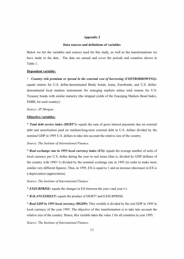
Dependent variable:

* Country risk premium or spread in the external cost of borrowing (COSTBORROWING):

equals returns for U.S. dollar-denominated Brady bonds, loans, Eurobonds, and U.S. dollar-

denominated local markets instruments for emerging markets minus total returns for U.S.

Treasury bonds with similar maturity (the stripped yields of the Emerging Markets Bond Index,

EMBI, for each country).

Source: JP Morgan.

Objective variables:

* Total debt service index (DEBT*): equals the sum of gross interest payments due on external

debt and amortization paid on medium/long-term external debt in U.S. dollars divided by the

nominal GDP in 1995 U.S. dollars to take into account the relative size of the country.

Source: The Institute of International Finance.

* Real exchange rate in 1995 local currency index (EX): equals the average number of units of

local currency per U.S. dollar during the year in real terms (that is, divided by GDP deflator of

the country with 1995=1) divided by the nominal exchange rate in 1995 (in order to make more

similar very different figures). Thus, in 1995, EX is equal to 1 and an increase (decrease) in EX is

a depreciation (appreciation).

Source: The Institute of International Finance

* EXSURPRISE: equals the changes in EX between the year t and year t-1.

* BALANCESHEET: equals the product of DEBT* and EXSURPRISE.

* Real GDP in 1995 local currency (RGDP): This variable is divided by the real GDP in 1995 in

local currency of the year 1995. The objective of this transformation is to take into account the

relative size of the country. Hence, this variable takes the value 1 for all countries in year 1995.


31

Control variables and instruments:

* Average emerging country risk premium or spread in the external cost of borrowing for the

emerging market asset class (EMBIWORLD): equals the stripped yields of the Emerging

Markets Bond Index, EMBI.

Source: JP Morgan.

* Exports (EXPORT): equals the total value of transactions arising from the export of goods and

services to nonresidents, valued at market prices in millions of U.S. dollars.


* Reserves excluding gold in 1995 U.S. dollars (RRES): equals official international reserves at

the end of the reporting year in millions of U.S. dollars, excluding gold, but including foreign

exchange, SDRs, and the reserve position in the IMF divided by the nominal GDP in 1995 U.S.

dollars (again, to take into account the relative size of the country).

Source: International Monetary Fund, International Financial Statistics.

* Factors affecting the risk to investment (CREDITORIGHTS): measure the quality of the

institutional setting affecting the risk of investment. The rating assigned is the sum of three

subcomponents, each with a maximum score of 4 and a minimum score of 0. A score of 4

indicates a very good environment for creditors and 0 a very poor. The subcomponents are:

contract viability/expropriation, profits repatriation and payment delays.

Source: International Country Risk Guide.

* Inflation (INFLATION): equals the yearly percentage change in the GDP deflator.


Balance sheet effects and the country risk premium: an empirical investigation

Documents

Transcript of Balance sheet effects and the country risk premium: an empirical investigation