Debt and Macro Stability:

by

Marc Jarsulic*

Working Paper No. 22

May 1989

Submitted to The Jerome Levy Economics Institute

Bard College

*Department of Economics, University of Notre Dame, Notre Dame, IN 46556

This research has been supported in part by The Jerome Levy Economics Institute, Bard College, Annandale-On-Hudson, NY. The views expressed are those of the author and do not necessarily reflect the views of The Levy Institute.

l_ Introduction

There has been much recent interest in the problem of fina.ncia.1

instability in the macro economy. Some researchers have looked for cyclical

and secular co-movements between debt accumulaticn., financial crises, and

problems in the real economy. Others have tried tr, rationalize, in formal

models, the apparent connections between finance, changes in expectations,

and macro inst%bility. Two different points of view are embodied in t&is

work. One, deriving from the work of Minsky, emphasizes the importance

of ignorance and psychology. Firms are seen as financing accu.mulation on

the basis of unverifiable expectations, accumula.ting debt burdens in the

process. When the debt burdens are large enough, the economy becomes

vulnerable to downward revisions of expectations. Su.ch revisions reduce

effective demand and stimulate financial crises. A second view emphasizes a.

structural determinant of instability -- declining profitability. Problems

with profits are viewed as a major cause of debt burdens, and the source of

potential financial crisis.

What follows is an attempt to synthesize these two viewpoints in a

manageable analytical framework. To set the stage, we begin with a brief

review of Minsky’s ideas, which have to this point received the grea&r

attention. This is followed by a discussion of the st.ructuralist. view and some

of the key supporting empirical evidence. Next a Keynes-Kalecki model of

growth with debt is constructed. It suggests that in economies where debt

fina.nces accumula.tion, stable and unstable configurations of economic

variables coexist simultaneously. The proximity of these regions is shown ti

depend an expectational and distributional factors. The model therefore

introduces a way to characterize financial fragility in terms of stability

theory, and shows how structuralist and Minskian ideas complement each

other.

2. Recent Work on Finance and Macro Stability

Minsky ( 1982) has long worked to develop a theoretica. connection

between debt and economic fluctuations. It is basically Keynesian is spirit.

He begins by looking at an economy at the end of a large scale depressio’n.

As a consequence of widely expefienced economic disaster, existing firms

will accept little debt, will prizs liquidity, and will make cautious estimates

of the potential profits from investment projects. Their rates of

accumulation will therefore be low, they will easily meet their debt

commitments, and gradually their confidence in the future will rise. Hence

they will raise estimates of future profitability, accept lower liquidity and

higher debt burdens., and increase rates of accumulation. This becomes a

self-reinforcing process which proceeds happily along until some event

disrupts the financial system. Minsky suggests that an increase in interest

fates is the usual culprit. In an economy where the demand for credit is

interest inelastic, because of high debt burdens, and where its supply is also

inelastic, because of policy of endogenous restrictions, the increase sparks a

crisis. The difficulty firms have in making debt payments causes them the

revalue the wisdom of investments. As investment demand declines, so do

profits, which amplifies the problem. The depth of the decline will depend

on how indebted firms are and how the goverment reacts. If the ultimate

downtu.rn is not ~JDO severe, it sets the stage for further expansion of debt

and larger problems in the future.

Now Minsky’s account is clearly driven by changes in expectations. Those

expectations are presumed to be formed in a Keynesian world,, that is where

the future is truly unknown; in which there are no contingent claim market.

for all enumerable eventualities; and in which actfirs have enough

experience to know that the future may generate events for which there is

no current. vocabulary. A neat, partial formulation of the Minsky view has

bsen prcjvided by Taylor and O’Connell ( 1%35). Using a linear dynamic

model, and making expected future profitability dependent on the deviation

of interest r&s from some normal value, they are able tfi show that ch&ges

household liquidity preference -- a proxy fGr confidence in the economy --

can switch the mc:jdel from a stable tfi an unstable state.

In the Minsky-inspired strand of analysis, variability of income shares

is not considered an important pal-t of the story. Recent empirical work

suggests this may be a significant omission. There is a long txadition of ne+

Martian research on the cyclical and b-end profit squeeze in the U. S.

economy (e.g. Boddy and Crotty, 1475; Weisskopf,, 1979; Hahnel and

Sherman, 1982; Gordon, Weisskllspf and Pxwles, 19 6 3). Recently Wolfson

( 1986~ made a very detailed study of financial crises in the post-war 11. S.

economy, using NBER business cycle dating techniques. He observed

(Wolfson, 1386, pp. 145-6) a regular relationship bet.ween changes in the

profit share and financial crisis:

In every crisis period, a pxticular timing relationship has -- witW

only one exception -- occurred. Peaks ha.ve been reached in profit. and

investment variables for the nonfinancial corporate sector, in relation

to the financial crisis, in the following order: C 1) the profit [share], i2>

new ox&acts and orders for plant and equipment (in constant

dollars), (3) investment and plant and equipment (in constant doltars),

(4) the financial crisis and (5) the financing gap [that is, the difference

between capital expenditures and internal funds]. (materials in

brackets added)

He concludes:

. . . t-&e financing gap increased in periods immediately preceding

financial crises not only because investment spending increased, But 1

also because internal funds declined. The failure of internal funds to

ma.intain their rate of growtA, in fact their tendency to decline,

resulted in an increasing financing gap...a decline in profits occurring

near the peak of We expansion generally has been responsible for this

decrease in inbrnal fundsAt was the decline in profits that resulted

in the corporations having difficulty in meeting their fixed payment

committ&Ients -- due TV involuntary plant and equipment investment

as well as debt.

Robert Pollin has looked at competing hypotheses which explain the

rising corporate debt in the post-war period. He concludes ( 1986, p.22 7)

that the increase is a function of declining profitability and competitive

pressure:

The overall results of the econometric test and other statistical

evidence point to one central conclusion: the trend decline in the

corporate profit level and rate over phase two, 1967-80, provides the

primary e,xplanation for the rise of corpora& debt dependency over

that period...With internal funds down, corporations were forced tfi

borrow tr, an increasing extent in order to maintain a competitive

level of spending and support their markets through trade credit

extensions.

The model developed in the subsequent section incofporates ideas fr6m

Minsky and from thi:tSe Who emphasize profitability. It Will be ?I.sed ti sh0W

why an economy with debt can have stable and unstable regions, and hbw

changes in expectational and structjJ.ral factfirs may iaffect the proximit)) of

those regions.

_ 3_ A Model of Accumulation with Debt

To keep life simple, we will begin witA a closed economy in which

aggregate demand., composed of investment and consumption, dekrmines

the rate of output. Goods markets ~411 be assumed to clear immediat&ly, and

money prices will be assumed fixed. To det..rmine flows of output we need

an investment function. This is always a difficulty for anyone const.ructing a

Keynesian-Kaleckian macro model. If the world is rea.lly cha.racterized by

ungrounded expectation s, how does one represent accumula.~ton as a.

function? Perhaps the best we can do is su.ggest that lcng term expectXii>ns

are given, but within the constraint of those expect-ations, scme functional

relationships obtain One common sense rela.tionship might be that capacity

u.t.ilization below a minimally acceptable level will exert downwa.rd pressure

on accumulation. Unless there is investment in innovative processes, t.here

will be no need to add to spare capacity. Another sensible step iS to carry

over some of the insights of Kalecki, which have reappeared in the so-called

“New Keynesian” li&ratu.re on fina.nce constiaints and accumulation (e.g.

Fazzari et a.l., NM). One begins with the not too startling assumption that

capital markets are not perfect. Lenders have difficulty evaluating

investment projecti, and have agent problems in monitoring and assessing

outcomes. Hence firms may be forced t’ wait for self -finance tc~ support

viable projects, and lenders may use cash-flow or indebtedness measures to

evalu.ate suitability of borrowers. Also, as Kalecki suggests, fifms may ‘knave

definite aversion tx bankruptcy risk, and thus restrict their use of finance a.s

cash-flow declines or debt rises. Hence, even when the Cheshire cat smile of

capitalists’ expectations is hanging firmly in place, variations in debt or cash-

flow will alter the rate of accumulation. This view will be represented by

writing the desired rate of capital accumulation, gd, as

where I’ is real output, K is real capital st.ock, n is the flow of profits divided

by the capital stock, r is the rate of interest, and d is the ratio of firm debt to

capital stock. This functional form is self-explanatory, will the exception of

the differing parameters (3 and v. This allows positive cash flows IX have a

negative effect on desired accumulation, which makes sense if dividends are

to be paid to stockholders and principal is to be retired. A larger relative

value of v would indicate a more cautious mood on the part of capitalists.

Since there are acknowledged lags between order and construction in the

capital good s sector, we will assume that the rate of accumulatWn, g = F;/K,

moves according to

will be no need to add to spare capacity. Another sensible step is tc carry

over some of the insights of Kalecki, which have reappeared in the so-called

“New Keynesian” literature on finance constraints and accumulation (e.g.

Fazzari et al., l%S>. One begins with the not too startling assumption that

capital markets are not perfect. Lenders have difficulty evaluating

investment projects, and have agent problems in monitoring and assessing

out_omes. Hence firms may be forced ti wait for self-finance to support

viable projects, and lenders rnay use cash-flow or indebtedness measures to

evaluate suitability of borrowers. Also, as Kalecki suggests, firms may have

definite aversion to bankruptcy risk, and thus restrict their use of finance as

cash-flow declines or debt rises. Hence, even when the Cheshire cat srnile of

capitalists’ expectations is hanging firmly in place, va.riations in debt or cash-

flow will alter the rate of accumulation. This view will be represented by

writing the desired rate of capital accumulation, gd, as

gd = a(Y,X - c) + J3n - ‘urd K, c, ~3, y > 0 , ~3 13

where Y is real output, K is real capital stock, p is the flow of profits divided

by the capital stock, r is the rate of inter-est, and d is the ratio of firm debt to

capital stock. This funCtiOna form is self-explanatory, will the eXceptiOn of

the differing parameters p and y. This allows positive cash flows to have a

negative effect on desired accumulation, which makes sense if dividends are

to be paid to stockholders and principal is to be retired. A larger relative

value of B would indicate a rnore cautious rnood on the part of capitalists.

Since there are acknowledged lags between order and construction in the

capital goods sector, we will assume that the rate of accumulation, g = i/K,

moves according to

k =h(gd-g -,-,gz), ~xbO,rpO (21

This is a standard part%.1 adjustment model with one innovation. The Mm

in g2 is added to fepJre%?nt an upper limit to the rate of growth. Even if gd -g

is large and positive, i will be limit&d by the current va.lue of g. Given this

relationship, we ne-xt turn our attention to the det&rmination of the debt

burden in this economy. It will be assumed that borrowing Qkes place only

to finance capital accumulation or make interest. pa.yments which ca.nnM be,

cOVered by ret&ed eXliingS. Thus we IiaW t.he relationship

b=rDtI-Bn (3)

where D is the real value of debt, I is investment, 1 > 8 x o is the corporat&

retention ratio, and l-I is the real value of profits. If corporate retained

earning always exceed investment eqJenbitures, there will be no debt.

Defining d= D/K, we have the identity

b = D/K - dg (4)

and substitution of (3) inti (41 gives

2 = rd + 8n - g - dg

The dynamical system given by (2 1 and (5) is tAe one which will be used

to analyze the ideas on finance and stability which were discussed in %he

previous section. This will be done in a series of cases, which make different

assumptions about income distribution, aggregate demand, and the

determination of the interest rate.

Case 1: Keynesian savings, interest rate and income shares fixed.

As a. first case consider an economy in which savings is proportional to

income, and in which la.bor’s share of income is taken to be determined

exOgeno?lsly by the relative power of workers and capitalists. Then capacity

utilization is given by . <

where s is the constant savings propensity. The rate of profit is

n=(l -w)g/s (7)

where w is labor’s share. The rate of interest will be taken as fixed. Now

this assumption may not be as strong as it seems. Unless one believes tha.t

the central bank can drive the long term rate of in&rest to zero, which

would imply unlimited funds for every borrower and a very lenient

capitalist system indeed, then it is likely that there is minimum rate of

interest on debt used to finance accumulation. So long as there is, the

following argument will go through. Expressions (6) and (7) can be

substitued into (2 ) and (5) to- obtain the corresponding dynamical system.

Assuming Q = [(CC + p( 1 - CO))&] - 1 > 0, which is necessary for g ever ~JD be

positive, and v = 1 - [8( 1 - d/s] > 0, which is necessary to explain the

existence of debt, we can write the dynamical system as

h = rd + vg - dg

where coefficients are implicitly redefined to account for the value of h. The

dynamics of (6) can be represented by the phase diagram given in Figure 1.

Assuming that (8) has two solutions, they will correspond to critical points A .

and B in the diagram. \

The motion around these pointz is indicatid in Figure 2, which ca.n be

derived from consideration of the vectors of motion given in Figure 1.

Clearly point A, with a lower rate of growth and higher debt capital ratio, is

locally a saddle point; while I3 is locally stable.1 Their juxtaposition suggests

the following intuitions about this model economy. Near point B, the

economy will respond to small enough shocks by oscillating about point B.

This might be taken to represent non-explosive business cycle behavior.

Larger shocks, however, might move the economy so far to the northwest

that it would begin to experience self -amplifying difficulties. Growth rates

would decline and debt burdens would increase. That is, a financial crisis

would develop.

Consider now the effects of a change in the distribution of income. An

increase in labor’s share would decrease profitability at every rat& of

accumulation, thus shifing the i = 0 isocline downward. Similarly, the

decline in profitability would shift t&e ‘d = 0 isocline upward, reflecting the

fact that for any rate of accumulation, more external finance would be

required. The net effect of these changes, iiiustuated in Figure 3, is to move

the stable point and the equilibrium point_ closer together. A shock which

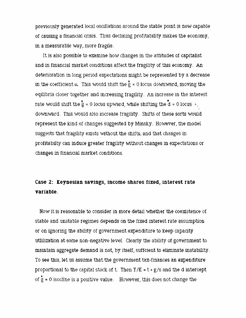
previously generated local QscillatiQns around the stable point is now capable

of causing a financial crisis. Thus declining profitability makes the ecQnQmy,

in a measurable way, mQre fragile.

It is alsQ pQssible to ey;amine how cha.nges in the attitudes of capitalist

and in financial market conditions affect the fragility of this economy. An

det&riQratiQn in long period c3p?Ct&iQnS might be represented by a decrease

in the cQefficient. CC. This WQUid shift the b = 0 ~QCUS downward, moving the

eqilibria clcrser tclgether and increasing fragility. An increase in the interest

rat& would shift the i = 0 locus upward, while shifting the & = 0 locus t I \

downward. This WQuld alsa increase fragility Shifts of these sclrts WQuld

represent the kind Qf changes suggest&d by Minsky. HQWeVer, the mQde1

suggests that ffagility exists without. the shifts, and that changes in

prQfitabilty can induce greater fragility withQut changes in expect&iQns or

changes in financial market cQnditiQns.

Case 2: Keynesian savings, income shares fixed, interest fate

variable.

NQW it is reasonable to consider in mQre detail whether the cQexist.nce Qf

stable and unstable regimes depends on the fixed interest rate assumption

Qr on ignoring the ability of gQvernrnent expenditure to keep ca.paCity

utlilization at sQme non-negative level. Clearly the ability of government to

maintain aggregate demand is not, by itself, suffcient to eliminate instability.

TQ see this, let us assume tha.t the government tax-finances an expenditure

prQpQrtiQna.1 to the capital stock of t. Then Y/K = t t g/s and the d intercept

of i = 0 isocline is a positive value. HQWeVer, this dQeS not change the

qualit&ve dynamics of the economy. Then what about a variable interest,

ra.te, together with aggregate dema.nd help from the government? To ma.ke

the rate of interest responsive to levels of demand, write a Keynesian

market clearing function for an exqenously given stock of money, M, as

This assumes an interest. sensitive transactions demand for money only. If

centWa1 S>ank policy is represented by M = mK, m > 0, t&e bank can dri+ the

in&rest rate up or down depending on how m changes. Then (9) can be

rewritten 8s

In t&is ca.se, unless m is infin&, a somewhat unlikely ba.nk policy, the ra%e

of interest is not Zer6. Substitution of ( 1 ct j intO (8 j will leave the dynamics

UliCfi~llgHi.

Case 3: Classical savings, income shares variable, interest fate

fixed.

As a final exercise with this model, let us consider the classical case,

where workers do not save, while ca.pitalisQ &I. If we choose to interpret

this in a Ka.leckian fashion, Y/K = g/C 1 -wj, and the rate of profit is equal to

the rate of accumulation. Here there is no possible impact of income shares

on We rati2 of borrowing. If some profits are distributed by corporat.ions and

capitalist households consume some part of diS&ibUted earnings, the

proportion of investment which will be financed is 1 - a/(( i-c)+c6) ) 0 ,

where 1 > c > 0 is capitalist propensity to consu.me from distributed profits

However, an increase in the wage share increases utilization rates, shifting

the i = 0 locus upward. This would make t1ie System less fragile.

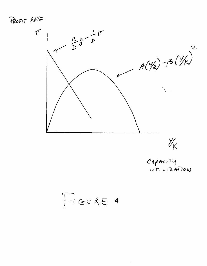
Since the elementary Kaleckian model does not accord with the behavior

of profit rates Over the business cycle, we need something slightly more

complex. Let us assume that possible rates of profit vary with the rate of

capxity utilization according to . \

This may be taken to reflect decreasing productivity as employment rates

increase along with capacity utilization. A relationship such as this is

suggest&d in the work c>f Gordon et al ( 1 M3). Let us also assume that , at a

given level of accumulation, aggregate demand will be related to profita.bility

according to

Y/K = cg - Dn C,bO WI

This reflects the fact that workers do not save while capitalists do. These

two relationships are represented in Figure 4. It is clear from this figu.re

that capacity utilization will increase with accumu.lation, but the profit rate

will increase and then decrease. Hence ( 11) and ( 12 > can be resM+d as

and

Y/K = J.Qg , y.3 > Q (l-4)

Substituticrn of ( 1.3) and ( 14) into (2) and (5) then gives us a dynamical

system of the form

b = rd + B(~i.~g - ~.~g2) - g - dg

This system is represented in the phase diagram of Figure 5 under the

assu.mptiion that ( 1 - Eljkl> j 0. In this case, there are now stable and unstable

points (If the &rm in bracket3 is less t&an zero there will be only an

unstable point.) In this system, changes in exI>ectWU-ial factors have the

same effects on the proximity of U-e stable and u.nstAble pointz 3.5 in 6%.

And a decrease in the potential profits at any rate of capacity utilizat&Xi,,

With would be representted by an decrease in the parameter kq, will shift

the i = 0 locus down and the ‘d = 0 locus up, thereby making this system

more fragile. Thus changes in potential profits have the same effects in all

three systems.

4 _ Conclusion

The model developed in the previous section provides a tractable

framework for examining the connection of debt to macroeconomic stability.

It shows that, under a va.riety of assu.mptions common tB the Keynes-Kale&i

tradition, an economy will have both stable and unstable regions. For some

combinations of growth rate and debt burden, an economy will be stable.

Shocks of a reasonable size may cause oscillations, but the economy will tend

toward acceptable values. For other growth rate-debt burden combinations

-- generally for lower growth rates and higher debt burdens -- the system

will be unstable. The closer these regions, the more vulnerable is the system

to shocks which move it away from the locally stable region.

The model therefore has the virtue of providing a definition of financial

fragility in terms of stability theory. The closer the stable and unstable

basins, the more financially fragile is t&e system. Moreover, since proximity

is determined by expectational, distributional, a.nd inter-est rate factors, the

model argues for a multivariate analysis of the causes of any financial crisis.

Finally, since some of the implications of the model are quite unambiguous, it

is gives potentially falsifiable form to some of the ideas in the financial

stability literature.

FootnotRs

1. While the stability properties can be deduced from the phase diagram,

they can be easily established algebraically in a particular case. Note that

for the dynamical system (6), which has a i = 0 isocline given by d = ($ - qg2

- c)/pr, the slope of the ‘g = 0 isocline is given by I$ - 2qg. To the left of g*=

$/Zq the slope is positive, and to the right it is negative. Note also that d > v

when2 = 0. Now the stability of a fixed point like A or I3 can be deriv?d

from the Jacobian matrix

evaluated at the fixed point (Arrowsmith and Place, pp. 85-6). When Det(Jj >

0 and Tr(Jj < 0, the point is stable. When Bet(J) < 0, it is a saddle. Taking the

derivatives of (8) gives the Jacobian

J =

v-d r-g

Now D&(J) = (4 - 2vg)(r - g) + /3r(v-d) = (4 - zqg>(r - g> + prv( 1-g/(g-r>j.

Therefore Det(J) > 0 if (I$ - zqg)(r - g)g - przd > 0. Substitution shows that.

this inequality is equivalent to 2qg3 + rc - qrg2 - 4g2 > 0. Since by

assumption g ) r, this can be reduced to g2(2qg - qr - 4) + rc ) 0. This will be

satisfied if g > ((I$ + qrj/2$. In the case where c = 0, (8) can be solved for g to

give an equilibrium value of g = {-(@+y) + [($+r)r)2 - 4qr(4 + v@11,2}/-27. If

g is to have two solutions, then it will be the case that the larger equilibrium

value of g will be greater than (4 + qr )/a?. The smaller value of g will be less

than this value. Hence A will be a saddle point, while B will be a stable

point. For cases in which t # 0, direct solutions for g require solving a cubic

equa.t.ion. Hence we are cont&nt with the qualitative analysis of the phase

diagrams.

Bibliogf aphy

Arrowsmith, D. and Place, C. 1982. Ordinary Differential Equations. New

York: Chapman and Hall.

Eocidy, J. and Crotty, R. 1975. Class Conflict and Macro Policy: The Political

Business Cycle. Review of Radical Political Economics, Spring.

Gordon, D., Weisskopf, T. and Bowles, S. 1983. Long Swings and We ‘I \

Nonreproductive Cycle. American Economic Review, May.

Fazzari, S., Hubbard, R., and Petersen, B. 1988. Financing Constraints and

Corporate Investment. Brookinps Papers on Economic Activity, Number 1.

Hahnel, R. and Sherman, H. 1962. The Rate of Profit Over the Business

Cycle. Cambridge Journal of Economics, June.

Minsky, H. 1982. Can “It” HaEpugain? Armor&, NY: M. E. Sharpe.

Pollin, R. 1966. Alternative Perspectives on the Rise of Corporate Debt

Dependency: The U. S. Postwar E,xperience. Review of Radical Political

Economics, Number 2.

Taylor, L. and 0’ Connell, S. 1985. A Minsky Crisis. Quarterly_Journal of

Economics, Supplement.

Wolfson, M. 1966. Financial Crises. Armor& NY: M. E. Sharpe.

.

.

\

8

!

, i !

3

*

i :

.

,

d :*

, I