Modeling the Macro-Economy of Bangladesh
76
Modeling the Macro-Economy of Bangladesh Final Report Prepared by Montague Lord, Staff Consultant Asian Development Bank January 2002
-
Upload
independent -
Category
Documents
-
view
0 -
download
0
Transcript of Modeling the Macro-Economy of Bangladesh

Modeling the Macro-Economy of Bangladesh Final Report Prepared by Montague Lord, Staff Consultant Asian Development Bank January 2002

MODELING THE MACRO-ECONOMY OF BANGLADESHA
Table of Contents Contents .............................................................................................................................. ii List of Tables .................................................................................................................... iv List of Figures ................................................................................................................... iv Acronyms ............................................................................................................................v Executive Summary......................................................................................................... vi 1.0 Introduction............................................................................................................1
1.1 Motivation for the Study.................................................................................1 1.2 Background and Modeling Methodology .......................................................1 1.3 Scope of the Study ..........................................................................................3
2.0 Characterization of the Economy.........................................................................5
2.1 Characteristics of the Data ..............................................................................5 2.2 Dynamic Specification....................................................................................8 2.3 Linking Poverty and Economic Growth .......................................................11
3.0 Modeling the Output Market..............................................................................14
3.1 Overview.......................................................................................................14 3.2 Output Determination ...................................................................................14 3.3 Aggregate Demand and the IS-Curve ...........................................................19 3.4 Aggregate Supply..........................................................................................21
4.0 Modeling the Monetary and Fiscal Sectors .......................................................23
4.1 The Supply and Demand for Money.............................................................23 4.2 Derivation of the LM Curve .........................................................................35 4.3 Government Revenue and Expenditures.......................................................26 4.4 Monetarization of the Fiscal Deficit .............................................................27
5.0 Modeling the External Sector .............................................................................28
5.1 Balance of Payments Components................................................................28 5.2 Demand for Imports......................................................................................31 5.3 Demand for Exports......................................................................................35 5.4 Overall Equilibrium ......................................................................................37
6.0 Modeling Economic Policies................................................................................40
6.1 Structure of the Model ..................................................................................40
- ii -
MODELING THE MACRO-ECONOMY OF BANGLADESHA
6.2 Specification of the Model............................................................................41 6.3 Aggregate Demand and Overall Equilibrium ...............................................43 6.4 Monetary Policy............................................................................................43 6.5 Fiscal Policy..................................................................................................45 6.6 Exchange Rate Policy ...................................................................................46
7.0 Projections and Policy Impact Assessments ......................................................48
7.1 Overview.......................................................................................................48 7.2 Baseline Forecasts.........................................................................................48 7.3 Fiscal Implications of Trade Liberalization..................................................51
8.0 Summary and Conclusions..................................................................................53 Annex: Model Listing in Eviews.....................................................................................54 References.........................................................................................................................65
- iii -

MODELING THE MACRO-ECONOMY OF BANGLADESHA
List of Tables Table 2.1 Descriptive Statistics of Key Macroeconomic Variables 6 Table 2.2 Poverty in Bangladesh, FY96-FY99 11 Table 2.3 Growth and Inequality Elasticities of Poverty in Bangladesh 12 Table 2.4 Comparative Poverty Elasticities 12 Table 3.1 Bangladesh: Value Added by Sector 21 Table 7.1 Major Baseline Assumptions, 2000-2010 48 Table 7.2 Baseline Projections of Key Macroeconomic Variables 50 Table 7.3 Poverty Changes in under Base Forecast 51 Table k7.4 Multiplier Analysis of Trade Liberalization on Key Macroeconomic Variables 52 List of Figures Figure 3.1 Real Effective Exchange Rate and Trade Volume Indices 19 Figure 3.2 The IS Curve 21 Figure 4.1 Velocity of M2 in Bangladesh 24 Figure 5.1 The FE Curve 30 Figure 6.2 Aggregate Demand and Output Equilibrium 38 Figure 7.1 Aggregate Output, Prices and the Exchange Rate 44
- iv -

MODELING THE MACRO-ECONOMY OF BANGLADESHA
Acronyms and Abbreviations
ADB Asian Development Bank ADF Augmented Dickey-Fuller ECM Error-correction mechanism ESAF Enhanced Structural Adjustment Facility DF Dickey-Fuller DW Durbin-Watson FE Foreign exchange IMF International Monetary Fund IS Investment-Savings MPC Marginal propensity to consume MPI Marginal propensity to invest MPX Marginal propensity to export REER Real effective exchange rate SAF Structural Adjustment Facility VAR Vector autoregressive
- v -

MODELING THE MACRO-ECONOMY OF BANGLADESHA
Executive Summary The present model provides a parsimonious representation of the macro economy of Bangladesh. It aims to serve a dual purpose. First, it provides a framework for making rational and consistent predictions about Bangladesh's overall economic activity, the standard components of the balance of payments, the expenditure concepts of the national accounts, and the financial sector balances. Secondly, it offers a means of quantitatively evaluating the impact of alternative policy reforms on the economy, and assessing the feedback effects that changes in key macroeconomic variables of the economy produce in other sectors. These two objectives are closely related since the capacity to make successful predictions depends on the model's ability to capture the interrelationships of the real and financial components of the economy. The modeling procedure described in this study has sought to account for the structure of the Bangladesh economy, the availability of data, and the degree of stability of time-series estimates of parameters. The nature of the modeling process of the Bangladeshi economy has motivated the design of a system that can grow and evolve with the economy. The present version of the model incorporates both the real and financial sectors of the economy within the existing exchange rate system. The objective is to provide a mechanism to link policies and targets while, at the same time, providing an easy and adaptable means of both forecasting key macroeconomic variables and simulating the interrelationships between economic policy initiatives. The present form of the model therefore provides a representation of the economy of Bangladesh that allows for considerable flexibility in its usage for forecasting, selection of the policy mix and instruments for the targets of a program, and determination of the appropriate sequencing of policy changes. The model applies a conventional framework to the economic system and, as a policy-oriented system, it incorporates key parameters for policy formulation. At the onset, the model is designed as a parsimonious representation of the underlying data generating system for key behavior relationships. The conceptual approach to the present model is based on conventional economic theory, although the empirical specification of the conventional theory is not well established since there are numerous approaches to the specification, estimation and testing procedures in standard macro models. The parsimonious nature of the model makes it tractable from an operational point of view, and it provides the basis for subsequent extensions of the public and financial sectors, as well as the domestic and external sectors of the economy. The study was undertaken by Montague Lord, ADB staff consultant, between July and October 2001. At the onset, discussions were held with government officials on macroeconomic policy and data availability, and documents and studies related to macroeconomic issues in Bangladesh were reviewed. Based on those data and reports, a macroeconomic model has been formulated using Eviews software. Simulations with the model are linked to an Excel spreadsheet to facilitate its use. This report contains the theoretical and empirical specification of the model, as well as sample forecasts and simulations.
- vi -
MODELING THE MACRO-ECONOMY OF BANGLADESHA
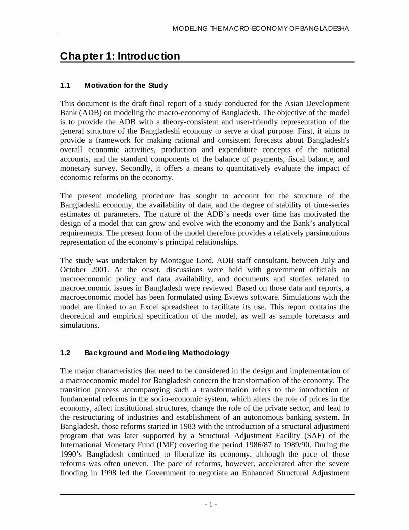
Chapter 1: Introduction 1.1 Motivation for the Study This document is the draft final report of a study conducted for the Asian Development Bank (ADB) on modeling the macro-economy of Bangladesh. The objective of the model is to provide the ADB with a theory-consistent and user-friendly representation of the general structure of the Bangladeshi economy to serve a dual purpose. First, it aims to provide a framework for making rational and consistent forecasts about Bangladesh's overall economic activities, production and expenditure concepts of the national accounts, and the standard components of the balance of payments, fiscal balance, and monetary survey. Secondly, it offers a means to quantitatively evaluate the impact of economic reforms on the economy. The present modeling procedure has sought to account for the structure of the Bangladeshi economy, the availability of data, and the degree of stability of time-series estimates of parameters. The nature of the ADB’s needs over time has motivated the design of a model that can grow and evolve with the economy and the Bank’s analytical requirements. The present form of the model therefore provides a relatively parsimonious representation of the economy’s principal relationships. The study was undertaken by Montague Lord, ADB staff consultant, between July and October 2001. At the onset, discussions were held with government officials on macroeconomic policy and data availability, and documents and studies related to macroeconomic issues in Bangladesh were reviewed. Based on those data and reports, a macroeconomic model has been formulated using Eviews software. Simulations with the model are linked to an Excel spreadsheet to facilitate its use. This report contains the theoretical and empirical specification of the model, as well as sample forecasts and simulations. 1.2 Background and Modeling Methodology The major characteristics that need to be considered in the design and implementation of a macroeconomic model for Bangladesh concern the transformation of the economy. The transition process accompanying such a transformation refers to the introduction of fundamental reforms in the socio-economic system, which alters the role of prices in the economy, affect institutional structures, change the role of the private sector, and lead to the restructuring of industries and establishment of an autonomous banking system. In Bangladesh, those reforms started in 1983 with the introduction of a structural adjustment program that was later supported by a Structural Adjustment Facility (SAF) of the International Monetary Fund (IMF) covering the period 1986/87 to 1989/90. During the 1990’s Bangladesh continued to liberalize its economy, although the pace of those reforms was often uneven. The pace of reforms, however, accelerated after the severe flooding in 1998 led the Government to negotiate an Enhanced Structural Adjustment
- 1 -

MODELING THE MACRO-ECONOMY OF BANGLADESHA
Facility (ESAF) with the IMF in exchange for foreign assistance. The ESAF included government revenue enhancement measures, reforms in the financial and public sectors, and privatization measures. Modeling these processes in Bangladesh requires the explicit recognition of how the transmission mechanism affects development on the real and financial sides of the economy. One approach is to incorporate uncertainty in the model and measure its effects on consumption and investment patterns. Another way is to include the propagation mechanism for the adjustment process on the cost side of the model, and use it to determine possible effects of incomes policies on price level increases and the rate of inflation. The inclusion of these transmission mechanisms is particularly important since there is general consensus that macroeconomic stabilization needs to be addressed early on in the reform process of economies in transition towards a market-oriented system. The movement towards more flexible market-determined prices in Bangladesh has also brought about fundamental changes in the way businesses and households respond to economic conditions. In modeling economic behavior, these changes imply a greater responsiveness of economic agents to changes in relative prices, and therefore possible parameter changes in the system of equations.1 If parameter changes occur, then the use of time-invariant parameters can make the system of equations unstable. The alternative approach consists of the introduction of time-varying parameters that capture the transition process in the structure of the economic system. These types of parameters can introduce an element of subjectivity in the operation of the model, and a decision to adopt time-varying parameters therefore should be approached with caution. Initial developments of macroeconomic modeling of transition economies were often based on the use of a vector autoregressive (VAR) system. More recently, the use of theory-consistent structural models, particularly those based on systems of dynamic time-series equations, has been found to forecast better for long horizons, especially when the equations take the form of the error-correction mechanism (ECM).2 As a result, a decision was made to develop a medium-size model for Bangladesh that would provide details as to the overall structure and operation of the economy, and which could be modified and expanded according to the needs of the ADB. This approach is a considerable expansion of earlier efforts to model the economy using a RMSM-type approach, which provided limited forecasting and simulation capabilities in a spreadsheet environment (ADB, 1991 and 1992). The present macroeconomic model aims to provide a theory-consistent representation of the general structure of the economy of Bangladesh and, as such, it offers real and financial sector forecasting and policy simulation capabilities targeted to the needs of the 1A parallel issue is that put forward under the Lucas (1976) critique of large-scale model that do not take into account changing expectations as policy rules change. Considerable progress has been made in addressing expectations variables that address Lucas' concerns, and the use of structural forward-looking models that take into account information updates by agents in their expectations generating equations. For an application of Hendry's (1988) distinction between forward-looking and backward-looking models, see Lord (1991). 2See, for example, Banerjee, Dolado, Galbraith, and Hendry (1993), Chapter 11, and references therein.
- 2 -

MODELING THE MACRO-ECONOMY OF BANGLADESHA
ADB. The model serves a dual purpose. First, it provides a framework for making rational and consistent predictions about overall economic activity in Bangladesh, the standard components of the balance of payments, and the production and expenditure concepts of the national accounts. Secondly, it offers a means of quantitatively evaluating the impact of exchange rate policies and other policy changes on the economy of Bangladesh, and assessing the feedback effects that changes in key macroeconomic variables of the economy produce in other sectors. These two objectives are, of course, closely related since the capacity to make successful predictions depends on the model's ability to capture the interrelationships between the real and financial sectors of the economy. The modeling procedure has sought to account for the structure of the economy of Bangladesh, the availability of data, and the degree of stability of time-series estimates of parameters during the country's transition process.3 The nature of the transition process of the economy of Bangladesh has motivated the design of a model that can grow and evolve with the economy. The present model therefore aims to provide a mechanism to link policies and targets while, at the same time, providing an easy and adaptable means of both forecasting key macroeconomic variables and simulating the interrelationships between economic policy initiatives. As such, the model provides a relatively parsimonious representation of the economy of Bangladesh that allows for considerable flexibility in its usage for forecasting, selection of the policy mix and instruments for the targets of a program, and determination of the appropriate sequencing of policy changes. 1.3 Scope of the Study This report is organized as follows: ♦ Chapter 1 explains the motivation for the construction of the model, and it provides a
general introduction to the macroeconomic framework of the Bangladeshi economy and past efforts to model it.
♦ Chapter 2 examines key time series of the Bangladeshi economy and dynamic
specification used to characterize economic relationships. ♦ Chapter 3 describes the modeling framework for the real sectors of the economy. ♦ Chapter 4 presents the modeling framework for the money market and fiscal sector. ♦ Chapter 5 sets forth the modeling framework for the balance of payments and the
foreign exchange market.
3For a recent application of this type of model to Eastern European and Central Asian economies, see Lord (1994) and Lord et al. (1995).
- 3 -

MODELING THE MACRO-ECONOMY OF BANGLADESHA
♦ Chapter 6 it describes the major blocks of the system of equations in the model, and it
explains the use of macroeconomic policy instruments under the system. ♦ Chapter 7 provides a baseline forecast and illustrates the impact of economic policy
reform measures on the economy. ♦ Chapter 8 provides a summary overview of the report. ♦ The Annex lists the model specification in the Eviews econometric software program
used to estimate and simulate the macroeconomic model. ♦ References lists the citations in the study.
- 4 -

MODELING THE MACRO-ECONOMY OF BANGLADESHA
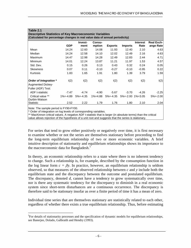
Chapter 2: Characterization of the Economy 2.1 Characterization of the Data The first step in modeling the economy of Bangladesh is to study the data-generating processes of key variables in the economy. In principle, one would expect that the long-term relationships between consumption and income, between investment and output, between imports of primary and intermediate products and output, between imports of final products and income would be cointegrated. Variables are said to be cointegrated if individually each is nonstationary but there exists a linear combination of the variables that is stationary. An error correction mechanism (ECM) can show how adjustments occur between variables to correct for short-term disequilibrium associated with the long-term equilibrium growth path of the variables. In the market-oriented system of the Bangladeshi economy, changes in prices, interest rates and exchange rates are generally not expected to impact on the long-run equilibrium growth path of the economy. Instead, the economy has a transient response to changes in these variables, and it is appropriate to constrain their long-term effects to zero.4 As such, it is important to differentiate between long-term equilibrium relationships of cointegrated variables, and the transient effects of changes in prices, interest rates, and exchange rates on the key macro variables in the present market-oriented economy. Table 2.1 presents some descriptive statistics of data series. The statistics on the first four moments (mean, standard deviation, skewness, excess kurtosis) refer to the change in the log of each variable since, if the variables are nonstationary, the statistics themselves will be nonstationary; moreover, the log change is an approximation of the percentage change, so that the minimum and maximums are the minimum and maximum percentage change of each variable, and the standard deviation is expressed as a percentage. The statistics generally follow the pattern of similar ones for developing and transition economies (see for example, Engel and Meller, 1993). For the national income account components, the standard deviations range from a low of 13 percent for consumption to a high of 43 percent for exports. The standard deviation for interest rates is much larger than that for the exchange rate. All the variables have excess kurtosis, indicating that the distributions have fat tails, and implying that there is a large probability of wide fluctuations, compared with those that would be expected from changes in series having a normal distribution. The tests reject normality for these variables.
4The intuitive explanation for limiting the effects of changes in prices, interest rates, and exchange rates on variables such as consumption and investment is that relative prices for goods cannot continue to deviate from one another since otherwise consumers will eventually purchase only the increasingly cheaper good; similarly, differences between the prices of the same good originating from different countries could not continue indefinitely without consumers eventually only purchasing the good from the country with the decreasing relative price for that product.
- 5 -
MODELING THE MACRO-ECONOMY OF BANGLADESHA
Table 2.1 Descriptive Statistics of Key Macroeconomic Variables (Calculated for percentage changes in real value data of annual periodicity)
GDP
Invest-ment
Consu-mption Exports Imports
Interest Rate
Real Exch-ange Rate
Mean 14.24 12.60 14.08 11.93 12.40 2.10 4.63 Median 14.24 12.58 14.10 12.02 12.49 2.16 4.63 Maximum 14.47 12.98 14.28 12.49 12.83 2.44 4.71 Minimum 14.01 12.24 13.87 11.21 11.97 1.53 4.57 Std. Dev. 0.15 0.26 0.13 0.43 0.32 0.24 0.05 Skewness 0.07 0.11 -0.10 -0.27 -0.10 -0.95 0.22 Kurtosis 1.83 1.65 1.91 1.80 1.39 3.79 1.59
Order of Integration * I(2) I(2) I(2) I(2) I(2) I(2) I(2)Augmented Dickey- Fuller (ADF) Test: ADF t-statistic -7.47 -4.74 -4.90 -5.67 -3.70 -4.26 -2.25 Critical value ** 1%=-4.89 5%=-4.35 1%=4.88 5%=-4.35 5%=-2.00 1%=3.05 5%=-2.00
Durbin-Watson Statistic 2.52 2.22 1.79 1.76 1.80 2.10 2.04
Note: The sample period is FY90-FY00.
* Order of integration on log levels of corresponding variables. ** MacKinnon critical values. A negative ADF t-statistic that is larger (in absolute terms) than the critical value allows rejection of the hypothesis of a unit root and suggests that the series is stationary.
For series that tend to grow either positively or negatively over time, it is first necessary to examine whether or not the series are themselves stationary before proceeding to find the long-term equilibrium relationship of two or more economic variables. A brief intuitive description of stationarity and equilibrium relationships shows its importance to the macroeconomic data for Bangladesh.5 In theory, an economic relationship refers to a state where there is no inherent tendency to change. Such a relationship is, for example, described by the consumption function in the log linear form c = βy. In practice, however, an equilibrium relationship is seldom observed, so that measures of the observed relationship between c and y include both the equilibrium state and the discrepancy between the outcome and postulated equilibrium. The discrepancy, denoted d, cannot have a tendency to grow systematically over time, nor is there any systematic tendency for the discrepancy to diminish in a real economic system since short-term disturbances are a continuous occurrence. The discrepancy is therefore said to be stationary insofar as over a finite period of time it has a mean of zero. Individual time series that are themselves stationary are statistically related to each other, regardless of whether there exists a true equilibrium relationship. Thus, before estimating
5For details of stationarity processes and the specification of dynamic models for equilibrium relationships, see Banerjee, Dolado, Galbraith and Hendry (1993).
- 6 -

MODELING THE MACRO-ECONOMY OF BANGLADESHA
the economic relationships in the model for Bangladesh, it is useful to determine whether the data generating process of each of the series is itself stationary. Since national account variables have a tendency to grow (positively or negatively) over time, the variables themselves cannot be stationary, but changes in those series might be stationary. Series that are integrated of the same order are said to be cointegrated and to have a long-run equilibrium relationship.6 For trending variables that are themselves non-stationary, but can be made stationary by being differenced exactly k times, then the linear combination of any two of those series will itself be stationary. It is therefore important to test the order of integration of the key series in the model. Tests for stationarity are derived from the regression of the changes in a variable against the lagged level of that variable. Consider the following simple levels regression: yt = a + byt-1 + d (2.1) where a and b are constants and d is an error term. If y is non-stationary, then b will be close to unity. By subtracting yt-1 from both sides, we obtain ∆yt = a + (b-1)yt-1 + d (2.2) The disturbance term d now has a constant distribution and the t-statistic on yt-1 provides a means for testing non-stationarity. If the coefficient on yt-1 is less than the absolute value of 1, then b must be less than 1, and y is therefore stationary. The Augmented Dickey-Fuller test is a test on the t-statistic of the coefficient on yt-1. The second test for non-stationarity is the Durbin-Watson (DW) test on the levels regression specified above. Since the DW statistically is given by DW = 2(1-r) (2.3) where r is the correlation coefficient between yt and yt-1, then y is white noise when r is zero. The DW is therefore 2 when y is stationary. In practice, when only a one-period lag of the dependent variable is included in the regression, then a Dickey-Fuller (DF) test is performed to determine whether the series is stationary. When first difference terms are included in the regression, then an Augmented Dickey-Fuller (ADF) test is performed. The number of lagged first difference terms to include in the regression should be sufficient to remove any serial correlation in the residuals, in which case the DW statistic should approximate 2. A constant and trend variable should be included if the series exhibits a trend and non-zero mean in the descriptive statistics. Alternatively, if the series does not exhibit any
6A series is said to be integrated of order k, denoted I(k), if the series needs to be difference k times to form a stationary series. Thus, for example, a trending series that is I(1) needs to be differenced one time to achieve stationarity.
- 7 -

MODELING THE MACRO-ECONOMY OF BANGLADESHA
trend but has a non-zero mean, only a constant should be included in the test regression. Finally, if the series appears to fluctuate around a zero mean, neither a constant nor a trend should be included in the test regression. Initially the test is performed on the levels form of the regression. If the test fails to reject the test in levels then a first difference test regression should be performed. If the test fails to reject the test in levels but rejects the test in first differences, then the series is of integrated order one, I(1). If, on the other hand, the test fails to reject the test in levels and first differences but rejects the test in second differences, then the series is of integrated order two, I(2). For real GDP of Bangladesh, for example, the following statistics are reported for the second difference of its log level, with an intercept
ADF Test Statistic = -7.49 The critical values for rejection of hypothesis of non-stationarity are as follows:
1% Critical Value* = -4 88 5% Critical Value = -3.42 10% Critical Value = -2.86
The test therefore failed to reject the test in levels and first differences but rejects the test in second differences, which indicated that the series is of integrated order I(2). The results of the ADF test and the DW test are presented in the bottom of Table 2.1. As expected, the tests all fail to establish stationarity of the log levels and indicate that all the log levels are integrated processes. In particular, investment, consumption, imports, and GDP are all of integrated order 2, as are exports, interest rates and the real exchange rate. To facilitate the presentation of the IS-LM framework used for policy analysis in Bangladesh, the behavioral equations have been presented in the levels form of the variables. However, empirical estimates in the levels form of the behavioral equations would yield parameters whose implied elasticities would vary over the historical and forecast period. In contrast, behavioral equations estimated in their log-linear form yield direct elasticity estimates whose values remain constant over both the historical and the forecast periods. The present estimates of the model for Bangladesh are therefore based on log-linear relationships. 2.2 Dynamic Specification The dynamic processes underlying adjustments of key economic variables to changes in their determinants are described by stochastic difference equations. The general form of the equation for any dependent variable Y and the explanatory variables Zi is: Yt = Σm
i=1 αi Yt-i + Σni=0 βi Zit + εt (2.4)
- 8 -

MODELING THE MACRO-ECONOMY OF BANGLADESHA
Like all dynamic equations, the stochastic difference equation imposes an a priori structure on the form of the lag to reduce the number of parameters that need to be estimated. Since national income account data of Bangladesh are limited in terms of their range and annual periodicity, the parsimonious representation of the data generating process afforded by the stochastic difference equation is advantageous to the modeling process. This class of equations has three other important advantages. First, as pointed out by Harvey (1991: ch. 8), the stochastic difference equation lends itself to a specification procedure that moves from a general unrestricted dynamic model to a specific restricted model. At the outset all the explanatory variables postulated by economic theory and lags of a relatively higher order are deliberately included. Whether or not a particular explanatory variable should be retained and which lags are important are decided by the results obtained. The approach is appropriate for an economy like that of Bangladesh where there is uncertainty about the explanatory variables to be included in the behavioral equation. The second advantage of the use of the stochastic difference equation lies in the estimation procedure. Mizon (1983) has noted that, given sufficient lags in the dependent and explanatory variables, the stochastic difference equation can be so defined as to have a white noise process in the disturbance term. As a result, the ordinary least squares estimator for the coefficients will be fully efficient. Finally, stochastic difference equations lend themselves to long-run solutions that are consistent with economic theory. This characteristic is useful for the present modeling framework for Bangladesh, which builds from theory to dynamic specification, and finally to estimation and testing of the theory. When restrictions are imposed by economic theory, the relationships between variables are determined by co-integration analysis, and equations known as error correction models are used to yield long-run solutions that are consonant with economic theory. Engle and Granger (1987) have demonstrated that a data-generating process of the form known as the error-correction mechanism (ECM) adjusts for any disequilibrium between variables that are cointegrated. The ECM specification thus provides the means by which the short-run observed behavior of variables is associated with their long-run equilibrium growth paths. Davidson et al. (1978) established a closely related specification know as the “equilibrium-correcting mechanism” (also having the acronym ECM) that models both the short and long-run relationships between variables. Rearranging the terms of a first-order stochastic difference equation yields the following ECM: ∆yt = αo + α1(y – z)t-1 + α2∆zt + α3zt-1 + vt (2.5) where -1 < α1 < 0, α2 > 0 and α3 > -1, and where all variables are measured in logarithmic terms.
- 9 -

MODELING THE MACRO-ECONOMY OF BANGLADESHA
The second term, α1(y – z)t-1, is the mechanism for adjusting any disequilibrium in the previous period. When the rate of growth of the dependent variable yt falls below its steady-state path, the value of the ratio of variables in the second term decreases in the subsequent period. That decrease, combined with the negative coefficient of the term, has a positive influence on the growth rate of the dependent variable. Conversely, when the growth rate of the dependent variable increases above its steady-state path, the adjustment mechanism embodied in the second term generates downward pressure on the growth rate of the dependent variable until it reaches that of its steady-state path. The speed with which the system approaches its steady-state path depends on the proximity of the coefficient to minus one. If the coefficient is close to minus one, the system converges to its steady-state path quickly; if it is near to zero, the approach of the system to the steady-state path is slow. Since the variables are measured in logarithms, ∆y and ∆z can be interpreted as the rate of change of the variables. Thus the third term, α2∆zt, expresses the steady-state growth in Y associated with Z. Finally, the fourth term, α3zt-1, shows that the steady-state response of the dependent variable Y to the variable Z is non-proportional when the coefficient has non-zero significance. Open economies, such as that of Bangladesh, have a long-term relationship with one or more series in the global economy after transient effects from all other series have disappeared. That part of the response of real GDP that never decays to zero is the steady-state response, while that part that decays to zero in the long run is the transient response. Examples of relationships in which steady-state responses occur are those between the real domestic private consumption and real GDP. An example of a transient response is exchange rate movements, since if relative price changes were not transient, the disparity between prices of the home country and the foreign market would continuously widen. In that case, consumers would eventually switch entirely to the supplier with the lower priced products. Hence, it is important to distinguish the short-run adjustment component from the long-run equilibrium component. The equilibrium solution of equation (2.5) is a constant value if there is convergence. Since the solution is unrelated to time, the rate of change over time of the dependent variable Y (given by ∆yt) and the explanatory variable Z (given by ∆zt) are equal to zero. However, in dynamic equilibrium, equation (2.5) generates a steady-state response in which growth occurs at a constant rate, say g. For the dynamic specification of the relationship in (A.4), if g1 is defined as the steady-state growth rate of the dependent variable Y, and g2 corresponds to the steady-state growth rate of the explanatory variable Z, then, since lower-case letters denote the logarithms of variables, g1 = ∆y and g2 = ∆z in dynamic equilibrium. In equilibrium the systematic dynamics of equation (2.5) are expressed as: g1 = αo + α1(y – z) + α2g2 + α3z (2.6) or, in terms of the original (anti-logarithmic) values of the variables: Y = k0 Zβ (2.7)
- 10 -

MODELING THE MACRO-ECONOMY OF BANGLADESHA
where k0 = exp{(-αo/α1) + [(α1 - α2α1 - α3)/ α1
2]g2}, and where β = 1 - α3/α1. The dynamic solution of equation (2.7) therefore shows Y to be influenced by changes in the rate of growth of Z, as well as the long-run elasticity of Y with respect to Z. For example, were the rate of growth of the explanatory variable accelerate, say from g2 to g’2, the value of the variable Y would increase. However, it is important to reiterate that the response to each explanatory variable can be either transient or steady-state. When theoretical considerations suggest that an explanatory variable generates a transient, rather than steady-state, response, it is appropriate to constrain its long-run effect to zero. 2.3 Linking Poverty and Economic Growth In April 2000 the ADB and the Government of Bangladesh signed the Partnership Agreement on Poverty Reduction (PAPR) (ADB, 2001). The Government’s emphasis on economic growth as a strategy to alleviate poverty is well founded on the large and growing empirical evidence that sustainable economic growth rates successfully lower poverty levels. Recent studies undertaken for a cross-section of countries by Dollar and Kraay (2000), Chen and Ravallion (2000), Gallup et al. (1998) and Lundberg and Squire (2000) have demonstrated that, on average, economic growth at the national level leads to a proportional growth in the incomes of the poor within those countries. The effectiveness of economic growth as an engine of poverty reduction, however, varies greatly across countries. We therefore need to determine the poverty reduction responsiveness to economic growth in a country such as Bangladesh to identify the kinds of economic policies that will be most conducive to reducing poverty. For Bangladesh, available data on the incidence of poverty in Bangladesh are derived from assessments undertaken by the Bangladesh Bureau of Statistics. According to the results of the Household Income and Expenditure Survey (HIES) 2000, the headcoupercent between FY92 and 2000.7 Over 80 perc
7 There are several indices for measuring poverty, the mospoverty gap, and the more complex Sen and Foster, Greerdictates that the measure used for quantitative poverty analheadcount index. The headcount index measure the pconsumption expenditures lies below the poverty line, w
- 11
Table 2.2Poverty in Bangladesh, FY96-FY99 FY92 2000 Change
Headcount Index:
Bangladesh, of which 58.8 49.8 -9.00
Rural Areas 61.2 53.0 -8.20
Urban Areas 44.9 36.6 -8.30Decomposition of Poverty Change
Bangladesh, of which - - -9.00
Rural Areas - - -6.84
Urban Areas - - -1.37
Migration - - -0.25
Inequality (Gini Coefficient)
Bangladesh, of which 38.8 41.7 2.9
Rural Areas 36.4 36.6 0.2
Urban Areas 39.8 45.2 5.4 Source: Headcount index from World Bank (1996) and MOP (1999); for decomposition of poverty change, see methodology explanation in text.
nt index fell from 58.8 percent to 49.8 ent of the poor are located in rural areas
t common of which are the headcount index, the and Thorbecke (FGT) indices. Data availability yses and policy evaluations in Bangladesh be the roportion of the population whose income or hich is defined as the cash equivalent of food
-

MODELING THE MACRO-ECONOMY OF BANGLADESHA
and the remaining poor are in urban areas. As a result, the incidence of rural poverty tends to dominate the national average. The dominance of the rural sector is apparent
Table 2.3 Growth and Inequality Elasticities of Poverty in Bangladesh
Explained by
Poverty
Elasticity Growth
Elasticity Inequality Elasticity
Pro-Poor Growth Index
Cambodia -0.87 -1.44 0.57 0.79
Rural Areas -0.82 -0.85 0.03 0.96
Urban Areas -1.09 -4.09 3.00 0.27 Source: See methodology explanation in text.
when we decompose the overall change in poverty into its rural, urban and migration components. The rural and urban components reflect the change in the rural and urban poverty incidence, weighted by their respective share of the total population. The migration component measures the movement from the rural area to urban areas, or visa-versa, and is weighted by the difference in the poverty incidence between the two areas.8 Table 2.2 demonstrates how the 9.0 percentage point decline in the overall poverty of Bangladesh was mainly attributed to the 6.84 percentage point decline in rural poverty. Migration to urban areas contributed a small portion of the decline. The nature of the poverty response economic growth can be ascertained from the effect on the rate of poverty reduction of the distribution-corrected rate of growth in average income.9 This effect can be measured, first, by calculating the overall responsiveness of poverty to changes in real per capita income and, second, by decomposing the effect into that portion associated with economic growth and that portion associated with income inequality (Table 2.3). The first calculation yields the ‘elasticity of poverty’, and is measured as the percentage change in absolute poverty incidence relative to the growth rate of income. Notationally, the poverty elasticity is θ = p/y, where θ denotes the elasticity of poverty, p is the percentage change in poverty incidence and y is the growth rate of real per capita income.
Table 2.4 Comparative Poverty Elasticities
Growth
Elasticity
Bangladesh -0.87
Cambodia -0.61 a/
Lao PDR -0.70 b/
Philippines -0.73 c/
India -0.92 c/
Indonesia -1.38 c/
Thailand -2.04 c/
Malaysia -2.06 c/
Taipei, China -3.82 c/ a/ Lord (2001) b/ Kakwani and Pernia (2000). c/ Warr (2001).
consumption providing at least 2,100 calories of energy (plus 58 grams of protein) per person per day, plus a small allowance for non-food consumption to cover basic items like clothing and shelter. Data from household socioeconomic surveys conducted in 1993-94 and 1997 have been used to estimate the headcount index. This index and the aforementioned alternatives measure material deprivation and excludes dimensions of poverty reflected in low achievements in education and health, and vulnerability and exposure to risk addressed most recently by the World Bank’s World Development Report 2000/2001 (World Bank, 2001a). 8 For a derivation of the equation for the change in poverty in terms of these three components, see Weiss (2001) and Anand and Kanbur (1985). 9 While the survey by Rodriguez C. (2000) finds little evidence on the role of inequality in determining economic growth, there is strong evidence that inequality can be harmful to long run economic growth by undermining economic reforms.
- 12 -

MODELING THE MACRO-ECONOMY OF BANGLADESHA
By way of contrast with other countries in the Asian region, Table 2.4 presents estimates by Lord (2001), Warr (2000) and Kakwani and Pernia (2000). These estimates underscore the moderate overall elasticity of Bangladesh relative to other countries. We can determine the extent of pro-poor policies in Bangladesh by differentiating between the effects on poverty associated with changes in aggregate incomes and those associated with changes in the distribution of that income. Kakwani (2000) has shown that changes in the incidence of poverty can be expressed as a simple additive function of (a) the effect associated with overall economic growth when the distribution of income does not change, and (b) the effect associated with changes in the distribution of income when overall growth does not change. The change in the absolute poverty incidence relative to the change in real per capita GDP growth, denoted θ, can therefore be decomposed into the pure economic growth component, θg, and the change in inequality component, θi:10
θ = θg + θi …(2.8) such that
dP/P = θgdY/Y + θidG/G …(2.9) where P is the incidence of poverty, Y is real per capita income, and G is the Gini coefficient. Since the estimated poverty elasticity is always equal to the (unadjusted) economic growth elasticity, we need to adjust the economic growth elasticity so that the sum of the calculated growth and inequality elasticities sum to that of the poverty elasticity. Kakwani and Pernia (2000, and references therein) derive their component elasticities by normalizing the observed growth and inequality elasticities so that they sum to the poverty elasticity. Using this approach for Bangladesh, we obtain the growth and inequality elasticities reported in Table 2.4. The growth elasticity is about average of those calculated for a cross-section of countries by Easterly (2000). We can incorporate these growth and inequality elasticities for rural and urban areas of Bangladesh into the macro model to show the linkages between economic growth projections and the incidence of rural and urban poverty in the country. Chapters 6 and 7 discuss the linkage and demonstrate their importance in a series of simulations of the model.
10 Datt and Ravallion (1992) provide a similar decomposition with an additional term that is excluded by Kakwani (2000) for computational ease.
- 13 -

MODELING THE MACRO-ECONOMY OF BANGLADESHA
Chapter 3: Modeling the Output Market 3.1 Overview The present model represents an application of the conventional Mundell-Fleming model using the IS-LM framework for the open economy of Bangladesh and, as a forecasting and policy-oriented system, it incorporates key parameters for the formulation of economic decisions. At the onset, the model is designed as a parsimonious representation of the underlying data generating system for key behavior relationships. A similar approach is adopted by the International Monetary Fund (IMF) staff's macroeconomic model-building applications and is used in IMF-sponsored adjustment programs, except that the underlying structure of those models are related to the monetary approach to the balance of payments (Frenkel and Johnson, 1976).11 The conceptual approach of the present model is instead based on conventional economic theory as described in standard textbooks such as Obstfeld and Rogoff (1997), Hall and Taylor (1997), Mankiw (1997), Barro (1997), and Sachs and Larrain (1993). The empirical specification of the conventional theory, however, is not well established since there are numerous approaches to the specification, estimation and testing procedures in standard macro models. Moreover, no one theory or dynamic specification can provide a complete description of the economy of Bangladesh. What is essential is that key features of the economic and financial process be represented in the system used to characterize the economy. The resulting system can therefore be viewed as an interpretation of the process by which real and financial transactions in the economy take place, and the way in which economic policies operate to affect those transactions. 3.2 Determination of Output To simplify the exposition that follows, Box 1 summarizes the notations used in the model. The present section describes the components for aggregate demand, and the output market in terms of the relationships for consumption, investment, government expenditures, exports and imports. Together these make up the Investment-Savings (IS)-curve. The following section examines factors effecting movements along the curve and those bringing about a shift in the curve.
11A description of the monetary approach to the balance of payments can be found in Frenkel and Mussa (1985); and Krugman and Obstfeld (1997). For a prototype IMF monetary model, see Khan and Montiel (1989); for a sampling of IMF macro models, see Khan, Montiel and Haque (1991).
- 14 -

MODELING THE MACRO-ECONOMY OF BANGLADESHA
Box 1 Notations in the Model
A = real domestic absorption Bb = overall balance of payments Bc = current account balance Bk = capital account balance Bt = trade balance C = real consumption expenditures Cg = real government consumption expenditures Cp = real private consumption expenditures D = domestic credit from the monetary sector Dp = domestic credit from the monetary sector to the private sector Dg = domestic credit from the monetary sector to the public sector Dgs = domestic credit from the monetary sector to the government En = nominal exchange rate Er = real effective exchange rate F = external debt of public sector, denominated in foreign currencies G = government expenditures Gr = government expenditures on other Gw = government expenditures on wages H = nominal debt of government I = real gross domestic investment expenditure If = foreign direct investment i = nominal interest rate if = nominal interest rate prevailing in world market K = stocks M = broad money N = real non-tax revenue of public sector P = domestic price level Pf = foreign currency price of goods purchased abroad r = real interest rate R = net foreign assets Rb = net foreign assets of commercial banks Rg = net foreign assets of government Rp = net foreign assets of private sector Tt = taxes from trade Tr = taxes from other sources V = velocity of money X = real exports Xs = export value of services Y = real aggregate demand Ya = real output of primary sector Yb = real output of secondary sector Yc = real output of tertiary sector Yd = real net household income Yf = real foreign market income Yg = real government revenue Z = real imports of merchandise Zs = import value of services
- 15 -
MODELING THE MACRO-ECONOMY OF BANGLADESHA
3.2.1 Aggregate Demand In an open economy, aggregate demand, Y, is the sum of domestic absorption, A, and the trade balance, B: Y = A + B (3.1) Domestic absorption measures total spending by domestic residents and public and private entities. It is composed of total private consumption, investment, and government expenditures: A = C + I + G (3.2) where C is real private consumption expenditure, I represents real gross domestic investment expenditures, and G is real government expenditures. The trade balance measures the net spending by foreigners on domestic goods. It is defined as: B = X - Z (3.3) where X denotes real exports, and Z represents real imports. As with domestic absorption, the trade balance is defined in real terms. 3.2.2 The Output Market Conventional IS-LM curves offer a useful analytical tool for examining the effects of policy initiatives or shocks on the Bangladeshi economy. These curves, along with that for foreign exchange (FE), provide a framework within which to show the equilibrium output solution of the Bangladeshi economy under different predetermined variables, including those representing policy instruments. We begin with the derivation of the IS curve, and in the next chapter derive the LM curve. After examining the fiscal component of the model, we derive the FE curve, and consider the effect of current account imbalances on capital flows, national savings and investment, and the Government’s budget deficit. There are four steps to the derivation of the IS curve. The first consists of the determination of the long run, or steady state, equilibrium solutions of the individual behavior relationships. The second involves the addition of the government's budget constraint to the system of equations. The third consists of the derivation of the reduced-form equation relating output to the predetermined variables in the economy. The final step consists of the determination of the relationship between interest rates and output to find the slope of the IS curve.
- 16 -

MODELING THE MACRO-ECONOMY OF BANGLADESHA
The steady state solution of a variable is a timeless concept. Thus for any variable Yt = Y = Yt-1. Similarly, ∆Yt = ∆Y = ∆Yt-1 is the rate of growth. In what follows, we present the steady-state solution for the behavioral equations that make up the system of equations in the model: Private Consumption is positively related to income and negatively related to interest rates. C = k1 + β11Y + β12r (3.4) The coefficient β11 is the marginal propensity to consume out of current income (MPC). In Bangladesh consumption by the private sector depends on income. As real interest rates have been negative in the early years of the sample period, the ratio of interest to inflation rather than the difference was used to make all values positive, thereby allowing the logarithm of all values in the series to be calculated. Nevertheless, the real interest rate measured in this form was not significant and of the right sign. The income elasticity is reasonable in magnitude and has the expected signs. Changes in income produce a strong impact on consumption in the same period, and then abate during subsequent years. Despite the relatively simple definition of income, the variable provided a reasonably good explanation of private consumption behavior in Bangladesh. The final equation using the ECM specification described in equation (2.5) is as follows12: ∆lnCt = 1.47 - 0.77 ln(C/Y) t-1 - 0.11 lnYt-1 (3.5) (11.2) (9.4)
R2 = 0.98 DW = 2.1 Period: 1992-2000 and the long-run, or steady-state solution, of the estimated equation is as follows: C = e3.6 Y0.85 (3.6) Hence the long-run elasticity of consumption with respect to income is 0.66 in the short run (after a one-period lag) and 0.85 in the long run. Investment is positively related to income and negatively related to interest rates and taxes. I = k2 + β21Y + β22r + β23T (3.7)
12 A binary variable (1 in 1998; 0 otherwise) was included in the equation to account for disruptions during the massive 1998 floods.
- 17 -

MODELING THE MACRO-ECONOMY OF BANGLADESHA
The coefficient β21 is the marginal propensity to invest out of current income (MPI). Investment in Bangladesh is composed of fixed investment and changes in stocks. Domestic economic activity in Bangladesh, the real domestic interest rates (lending rate), and taxes were included as explanatory variables. While total taxes entered the equation with a statistically significant coefficient, trade taxes had a greater power of explanation of investment movements. The final equation is as follows:13
∆lnIt = -11.3 - 0.73 ln(I/Y) t-1 + 0.70 lnYt-1 - 0.06∆ln r t-1 – 0.03 ln r t (3.8) (5.7) (4.5) (5.1) (2.0)
R2 = 0.99 DW = 3.5 Period: 1993-2000 The elasticity of investment with respect to income is 1.96 in the long run; with respect to the real interest rate it is -0.06 in the short run and -0.04 in the long run. Exports are positively related to foreign market income and negatively related to both the price of exports and the real exchange rate. X = k4 + β41Yf + β42 Pn+ β43er (3.10) The coefficient β41 is the marginal propensity to export out of foreign market income (MPX). The price effect in equation (3.10) is decomposed into the own-price effect, measured in terms of the domestic currency, and the real effective exchange rate (REER) effect. The REER takes into account changes in the price of domestic goods, Pn, relative to that of foreign goods, Pf, and the nominal exchange rate, Rn. At the bilateral trade level, the real exchange rate is measured by the ‘real cross-rate’, which takes into account changes in the nominal exchange rate of Bangladesh with the foreign country and the relative price levels between Bangladesh and that country. The decomposition allows us to separate the own-price (transmitted through their effect on the domestic-currency-denominated price level) and cross-rate effects to measure the impact of changes in both trade taxes and the exchange rate on the balance of trade and the macro-economy. Estimates of equation (3.10) for Bangladesh are presented in Chapter 5. Imports are positively related to domestic income and the real exchange rate, and they are negatively related to the price of imports. Zt = k5 + β51Y + β52P + β53er (3.11) The coefficient β51 is the marginal propensity to import out of domestic income (MPM). The price effect is decomposed into the foreign currency denominated import price, P,
13 binary variable (1 in 1998; 0 otherwise) was included in the equation to account for disruptions during the massive 1998 floods.
- 18 -
MODELING THE MACRO-ECONOMY OF BANGLADESHA
and the real effective exchange rate, er.14 The equation estimates for
swd(wa
Figure 3.1
P
tde
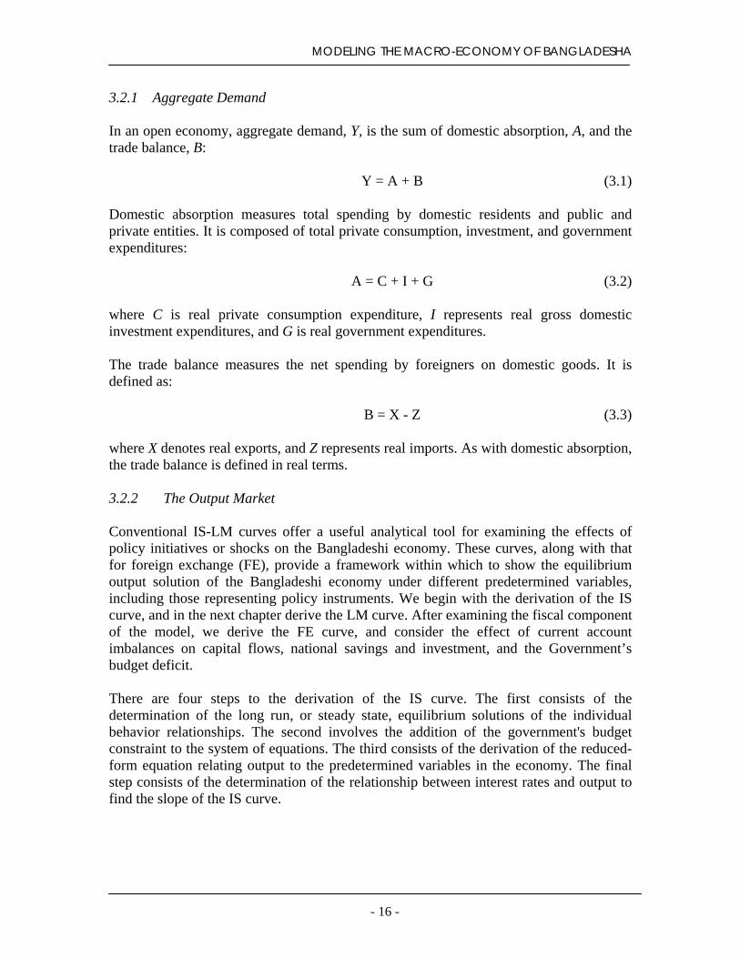
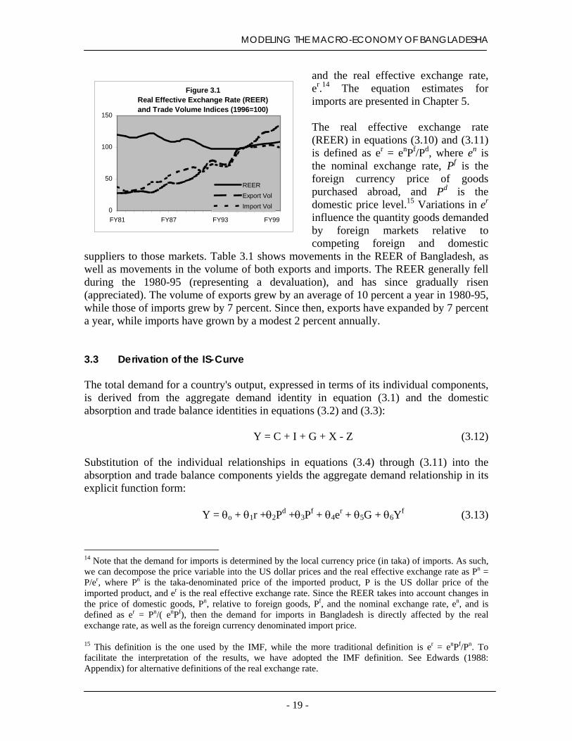
imports are presented in Chapter 5. The real effective exchange rate (REER) in equations (3.10) and (3.11) is defined as er = enPf/Pd, where en is the nominal exchange rate, Pf is the foreign currency price of goods purchased abroad, and Pd is the domestic price level.15 Variations in er influence the quantity goods demanded by foreign markets relative to competing foreign and domestic
uppliers to those markets. Table 3.1 shows movements in the REER of Bangladesh, as ell as movements in the volume of both exports and imports. The REER generally fell uring the 1980-95 (representing a devaluation), and has since gradually risen appreciated). The volume of exports grew by an average of 10 percent a year in 1980-95, hile those of imports grew by 7 percent. Since then, exports have expanded by 7 percent
year, while imports have grown by a modest 2 percent annually.
Real Effective Exchange Rate (REER) and Trade Volume Indices (1996=100)
0
50
100
150
FY81 FY87 FY93 FY99
REERExport VolImport Vol
3.3 Derivation of the IS-Curve The total demand for a country's output, expressed in terms of its individual components, is derived from the aggregate demand identity in equation (3.1) and the domestic absorption and trade balance identities in equations (3.2) and (3.3): Y = C + I + G + X - Z (3.12) Substitution of the individual relationships in equations (3.4) through (3.11) into the absorption and trade balance components yields the aggregate demand relationship in its explicit function form: Y = θo + θ1r +θ2Pd +θ3Pf + θ4er + θ5G + θ6Yf (3.13)
14 Note that the demand for imports is determined by the local currency price (in taka) of imports. As such, we can decompose the price variable into the US dollar prices and the real effective exchange rate as Pn =
/er, where Pn is the taka-denominated price of the imported product, P is the US dollar price of the imported product, and er is the real effective exchange rate. Since the REER takes into account changes in he price of domestic goods, Pn, relative to foreign goods, Pf, and the nominal exchange rate, en, and is efined as er = Pn/( enPf), then the demand for imports in Bangladesh is directly affected by the real xchange rate, as well as the foreign currency denominated import price.
15 This definition is the one used by the IMF, while the more traditional definition is er = enPf/Pn. To facilitate the interpretation of the results, we have adopted the IMF definition. See Edwards (1988: Appendix) for alternative definitions of the real exchange rate.
- 19 -

MODELING THE MACRO-ECONOMY OF BANGLADESHA
where θ1 < 0, θ2 < 0, θ3 < 0, θ4 > 0, θ5 > 0, θ6 > 0. Aggregate demand is therefore negatively related to the real interest rate and domestic and foreign trade prices, and positively related to, the real exchange rate, government expenditures, and foreign market income. The total effects of a change in interest rates, government expenditures, the real exchange rate, and foreign income are given by the corresponding coefficients of these variables in equation (3.13). An increase in foreign income, Yf, for example, causes aggregate domestic income, Y, to increase by an amount that is always greater than the original increase in foreign economic activity. The increase in foreign income initially increases exports, which expands domestic aggregate income. The expansion then increases consumption and investment, though there is also some leakage from the accompanying increase in imports. That expansion then leads to a further increase in consumption and investment, thereby leading to a new round of aggregate income increases, until the full impact of the increase in foreign income has been completed. Hence, a unit increase in foreign income always leads to a more than proportional increase in aggregate domestic income. Similar multiplier effects occur with change in interest rates, domestic and foreign trade prices, government expenditures, and the real exchange rate. In each case, the final effect on aggregate demand is more than proportional to the change in these variables. The effect of a change in the real exchange rate on aggregate demand, however, is less clearly defined. For a relatively small country like Bangladesh, the Law of One Price will ensure that the demand curve for traded goods is perfectly elastic, so that a devaluation will shift the export demand curve in proportion to the devaluation if there is underutilization of capacity. There is a large literature on possible contractionary effects of a devaluation of output (for a survey, see Lizondo and Montiel, 1989). Edwards has summarized the theoretical reasons for contractionary devaluations (1991: 311-330). They arise from the effects that a devaluation can have through either price rises that cause a negative real balance effect, the redistribution of demand from a sector having a low marginal propensity to save to one with a high one, low price elasticities of demand for exports and imports, or supply-side rigidities. The IS (investment-savings) curve relates the level of output of Bangladesh to its real interest rate. The IS curve is obtained from the relationship between the level of aggregate demand and the level of the interest rate in equation (3.13): ∆r/∆Y = 1/θ1 < 0 (3.14) The curve relating the level of aggregate demand to the level of interest rates is therefore downward sloping. Shifts in the IS curve result from changes in domestic and foreign trade prices, the real exchange rate, government expenditures, and foreign income. An increase in the real exchange rate causes both foreign and domestic residents to shift their consumption to relatively less expensive Bangladeshi goods, causing aggregate demand to rise and the IS
- 20 -

MODELING THE MACRO-ECONOMY OF BANGLADESHA
curve shifts to the right for the given level of
3ti
TB V
V
V
GS
interest rates. The amount by which the curve shifts is ∆Y/∆er = θ2 > 0. A similar rightward shift in the IS curve occurs when there is an increase in foreign market income, and the amount by which aggregate demand increases equals ∆Y/∆Yf = θ4 > 0. For government expenditures, the increase in aggregate demand equals ∆Y/∆G = θ3 > 0. These shifts are demonstrated in Figure
.2. If we were to include taxes, an increase in taxes would reduce disposable income, hereby lowering consumption and shifting the IS curve to the left for the given level of nterest rates. The amount of the shift would be given by ∆Y/∆T = θ5 < 0.
Figure 3.2 The IS Curve
IS
∆ Y/ ∆ e r
∆ Y/∆ Yf
∆ Y/∆ G
∆ Y/ ∆ T
Y
i
3.4 Aggregate Supply Having determined aggregate demand, we need to find aggregate supply to determine the output of the economy. Aggregate supply is given by the value added by each sector. The value added of all industries in a sector is the sum of the difference between their total revenue and the cost of their purchases from other industries or firms. In the present model, the output levels of both the primary and tertiary sectors are endogenous, while the secondary sector is predetermined.
able 3.1 angladesh: Value Added by Sector (percent contribution)
FY90 FY91 FY92 FY93 FY94 FY95 FY96 FY97 FY98 FY99 FY00 alue Added: Primary Sector 30% 30% 29% 26% 26% 26% 26% 26% 25% 26% 26%
alue Added: Secondary Sector 21% 22% 22% 24% 24% 25% 25% 25% 26% 25% 25% of which: manufacturing 13% 13% 14% 15% 15% 15% 15% 16% 16% 15% 15%
alue Added: Tertiary Sector 48% 48% 48% 50% 50% 49% 49% 49% 49% 49% 49%
DP at factor costs 100% 100% 100% 100% 100% 100% 100% 100% 100% 100% 100%
ources: Bangladesh Bureau of Statistics and World Bank.
In modeling the value added of these three sectors, we determine the output level of secondary sector by the economy's overall expenditure level and the activity of the other two sectors. Output of the primary sector, measured in 1991 taka, is a positive function of aggregate investment, I, and the real exchange rate:
- 21 -

MODELING THE MACRO-ECONOMY OF BANGLADESHA
Yb
t = α60 + α61It + α62er t + µ6 (3.15)
The final equation in its ECM form is as follows16: ∆lnYb
t = 3.3 - 0.83 ln(Yb/I) t-1 -0.50 ln It-1 + 0.64 ln er t-1 (3.16)
(2.4) (2.0) (2.0)
R2 = 0.77 DW = 2.8 Period: 1991-2000 The elasticity of primary sector activity with respect to gross fixed capital formation is 0.33 in the short run and 0.4 in the long run. With respect to the real exchange rate, it is 0.64 in the short run (after a one period lag) and 0.85. in the long run. Similarly, the output of the tertiary sector is a positive function of gross fixed capital formation, I, and the real exchange rate: Yc
t = α63 + α64It + α65er t + µ6 (3.17)
and the estimated equation is:17
∆lnYc
t = 4.0 - 0.67 ln(Yc/I) t-1 + 0.59∆lnI t - 0.27 lnI t-1 (3.18) (2.9) (7.8) (2.7)
R2 = 0.96 DW = 1.7 Period: 1991-2000 The elasticity of tertiary sector activity with respect to gross fixed capital formation is 0.6 in both the short run and long run.
16 A binary variable was included for 1995 (1 in 1995; 0 otherwise). 17 A binary variable was also included for 1993-94 (1 in 1993 and 1994; 0 otherwise).
- 22 -

MODELING THE MACRO-ECONOMY OF BANGLADESHA
Chapter 4: Modeling the Monetary and Fiscal Sectors 4.1 Overview The banking system of Bangladesh is composed of the Bangladesh Bank as the central bank and a commercial banking system that is regulated by the Bangladesh Bank. The Bangladesh Bank controls the monetary base, or supply of currency in circulation and commercial bank reserves, through a set of policy instruments that are gradually evolving in importance. The current limitations on international movements of capital imply that the growth of the money supply is closely related to the domestic component of the stock of money. In general, the domestic money stock is made up of net foreign assets of the consolidated banking system, plus bank credit to the public and private sector. Thus, control over capital movements has allowed the Bangladesh Bank to focus on the domestic stock of money component. In general, money is classified into the following categories:
• High-powered money is made up of currency in circulation plus cash reserves of commercial banks in the Bangladesh Bank.
• M1 money consists of liquid assets that include currency, demand deposits, traveler's checks, and other types of deposits against which checks can be drawn.
• M2 money, or broad money, is composed of M1 plus quasi money such as savings deposits and money market deposits.
4.1.1. The Supply of Money The supply of money is composed of taka and foreign currency liquidity. The level of this liquidity equals M2, denoted M, and is composed of (a) net domestic assets, denoted D, and net foreign assets, denoted R (in domestic currency terms). Hence: Mt = Rt + Dt (4.1) where net domestic assets is given by: Dt = Dp
t + Dgt (4.2)
and net foreign assets is made up of net foreign assets of the Bangladesh Bank, denoted Rc, net foreign assets of commercial banks, denoted Rb, net foreign assets of the private sector, denoted Rp, and net foreign assets of the government, denoted Rg: Rt = Rc
t + Rbt + Rp
t + Rgt (4.3)
- 23 -

MODELING THE MACRO-ECONOMY OF BANGLADESHA
The velocity of money defines the number of times that the each unit of money circulates in the economy each year. For M2 money, the velocity of money, denoted V2, is defined as: V2 = YP / M2 (4.4) If V2 is relatively constant and real output, Y, is determined by other factors, then the
supply of money, M, should grow in a fixed proportion to Y to keep prices, P, stable, since equation (4.4) implies that P = MV/Y. These circumstances generally describe the monetarist doctrine, under which a stable growth of M precludes the use of a proactive monetary policy. In Bangladesh, however, V2 has not remained constant but rather declined, and under appropriate conditions, monetary policy can play an
important role in the economy.
Figure 4.1Velocity of M2 in Bangladesh
2.0
3.0
4.0
5.0
FY90 FY95 FY00
4.1.2. The Demand for Money The conventional approach to the demand for money derives from the Baumol-Tobin model (for details, see Obstfeld and Rogoff, 1997; Farmer, 1998; Hall and Taylor, 1997; Mankiw, 1997; Barro, 1997; and Sachs and Larrain, 1993). It defines the demand for money in an analogous way as the demand for stocks by companies. Money, like stocks, is held by individuals and firms to ensure that they have the necessary liquidity to pay for goods and services. Thus as income expands, the demand for money increases; as income contracts, money demand decreases. There is, however, an opportunity cost associated with holding money and associated with foregone earnings from holding interest-bearing financial assets such as bonds. The desire to hold money is therefore negatively related to the interest rate. As interest rates rise, the opportunity cost of holding money increases and the demand for money expands; as interest rates fall, the demand for money contracts due to the lower opportunity cost incurred from holding money. The aforementioned relationships between the demand for money and both income and interest rate are specified in real terms, since the demand for money is generally considered to be absent of any money illusion. Variations in prices therefore lead to proportional changes in nominal income, interest rates, and money demand.
- 24 -

MODELING THE MACRO-ECONOMY OF BANGLADESHA
The demand for money, M, is therefore defined in terms of real balances, M/P, and it relates the demand for those balances to the real rate of interest, r, and the level of income, Y: M/P = k70 + β71r + β72Y (4.5) The coefficient β71 is used to measure the interest elasticity of money demand, and the coefficient β72 serves to measure the real-income elasticity of money demand. In Bangladesh, the final price equation that we derive from equation (4.5) is as follows: ln Pt = 0.97 + 0.13 ln(M/Y) t-1 + 0.84ln(P)t-1 (4.5’) (1,8) (9.3)
R2 = 0.99 DW = 2.0 Period: 1991-2001 In Bangladesh the official rate of inflation has decelerated from over 20 percent a year in the early 1990s to around 4 percent by the end of the decade. However, the rate is affected by rigidity of prices in subsidized goods and fixed rents that enter into the consumer basket. 4.2 Derivation of the LM Curve The LM curve relates the level of aggregate demand to the interest rate for a given level of real money balances. Thus, at each point in the curve, the aggregate demand associated with a given interest rate is consistent with money market equilibrium. The LM curve is found from the steady-state equilibrium solution of equation (4.1) and equation (4.5) in terms of interest rate: r = κ0 - κ1Y + κ2(enR+D)/P (4.6) where κ0 = k'7, κ1 = (β72/β71), and κ2 = (1/β71). The slope of the LM curve is given by: ∆r/∆Y = - κ1 (4.7) Since κ1 = β72/β71, and β71 < 0 and β72 > 0, the slope of the LM curve is positive. A higher interest rate lowers the demand for money and a higher aggregate demand increases the demand for money. Hence, for a given real money balance, M/P, money demand can only be equal to the given money supply if an increase in interest rates is matched by an increase in aggregate demand. Increases in the money supply, say from an increase in net foreign assets, R, shifts the LM curve to the right. When the money supply expands, it creates an excess supply of
- 25 -

MODELING THE MACRO-ECONOMY OF BANGLADESHA
money at the prevailing interest rate and level of output. The excess supply causes households to convert their money to bonds and other securities, which drives down the interest rate. The lower interest rate, in turn, increases investment and leads to an overall expansion in aggregate demand. 4.3 Government Revenue and Expenditures The Government’s revenue collection has been hindered by the large informal sector and dependence on foreign trade taxes. As a result, the real value of tax revenue collections has grown by less than 1 percent on average since 1992. In order to reduce the overall budget deficit, government expenditures have had to be cut, especially on non-wage expenditures. While the burden of the budget deficit as a percentage of GDP has been reduced from 18 percent in 1990/91 to 5 percent in 1998/99, government investment activities, particularly in public infrastructure, have suffered. In addition to public sector wage payments, there has been a drain on government budget from the need to finance public sector programs. Taxes from trade, denoted Tt, are calculated from the level of imports and the average tariff rate. Other taxes, denoted To, is related to private consumption: ∆ln To
t = -1.11 - 0.67 ln(To/Y) t-1 (4.8) (3.0)
R2 = 0.65 DW = 1.2 Period: 1992-2000 Current government expenditures are separated into wages and other expenditures. Expenditures on wages, denoted Gw, are related to private consumption: ∆ln Gw
t = -1.26 - 0.50 ln(Gw/Cp) t-1 (4.9) (4.1)
R2 = 0.85 DW = 3.2 Period: 1994-2000 Other government expenditures, denoted Gr, are related to total government revenue: ∆ln Gr
t = -0.28 - 0.51 ln(Gr/Yg) t-1 (4.10) (1.6)
R2 = 0.55 DW = 2.1 Period: 1994-2000
- 26 -
MODELING THE MACRO-ECONOMY OF BANGLADESHA
4.4 Monetarization of the Fiscal Deficit The fiscal deficit, or the change in the government's debt, is the difference between the government's current expenditures and revenue. Government expenditures consist of nominal expenditures on domestic goods, PG, interest payments on domestic debt, it Dg
t-
1, and interest payments on foreign debt, it Ft-1. The government revenues derive from tax receipts (in nominal terms), PT, and income from capital and other sources (in nominal terms), PN. The difference between revenue and expenditures represents the change in government debt: ∆Dg
t = PG + it Dgt-1 + it Ft-1 - PT - PN (4.11)
The change in the government debt can be financed through an increase in the money supply, ∆Mt, a decrease in foreign exchange reserves, en
t∆Rt, an increase in the amount borrowed from the private sector, ∆Dp
t, or an increase in the amount transferred from extra-budgetary funds, ∆Dgr
t. These sources of deficit financing can be derived from the money supply equation (4.1) and equation (4.3): ∆Dg
t = ∆Mt - ent∆Rt - ∆Dp
t - ∆Dgrt (4.12)
The government budget relates the sources of the deficit in equation (4.12) to the financing of the deficit in equation (4.11): PG + it Dg
t-1 + it Fgt-1 - PT - PN = ∆Mt - en
t∆Rt - ∆Dpt - ∆Dgr
t (4.13) The budget constraint in equation (4.14) states that the government can finance its deficit by increasing the money supply, borrowing from the public sector, or reducing its foreign exchange holdings.
- 27 -

MODELING THE MACRO-ECONOMY OF BANGLADESHA
Chapter 5: Modeling the External Sector 5.1 The Balance of Payments The principal components of Bangladesh’s current account balance are made up of the individual balances on goods and non-factor services18, income19 and transfers20. Any deficit arising in the current account represents an imbalance between national savings and investment that needs to be financed by a capital inflow or the accumulation of debt. Offsetting financial cash flows in the capital account arise from foreign direct investment, portfolio investment and other investments, and any imbalance between the current and capital accounts of the balance of payments must be financed through changes in the official foreign reserves of Bangladesh. Traditionally, interest in the capital account has focused on FDI flows, which comprise capital transactions such as equity capital, earnings reinvestment, and other short and long-term capital that is used to acquire management interest in an enterprise operating in Bangladesh. Portfolio investments comprising long-term bonds and corporate equities other than direct investment and reserves have become important to Bangladesh since the mid-1990s. Financing of the current account deficit with portfolio investment tends to be less sustainable than a deficit financed by FDI flows since these so-called hot money flows are more sustainable to reversals when market conditions and sentiments change. 5.1.1 Balance of Payments Equilibrium Overall equilibrium in the balance of payments is the sum of the trade balance, B, and the balance in the capital account, K:
Bb
t = Bt + Kt (5.1)
The capital account is mainly associated with movements in FDI, which in turn depend on interest rates and foreign and domestic incomes. Using equation (3.10) for exports and
18Non-factor services comprise shipment, passenger and other transport services, and travel, as well as current account transactions not separately reported. These include transactions with nonresidents by government agencies and their personnel abroad, and also transactions by private residents with foreign governments and government personnel stationed in Bangladesh. 19This balance comprises income from (a) factor (labor and capital) services in the form of income from direct investment abroad, interest, dividends, and property and labor income; and (b) long-term interest on the disbursed portion of outstanding public and private loans repayable in foreign currencies, goods or services. 20Transfers include (a) private net transfer payments between private persons and nonofficial organizations of the reporting country and the rest of the world that carry no provisions for repayments and that include workers' remittances, transfers by migrants, gifts, dowries, and inheritances, and alimony and other support remittances; and (b) official net transfers in the form of payments between the GOE and governments of the rest of the world.
- 28 -

MODELING THE MACRO-ECONOMY OF BANGLADESHA
equation (3.11) for imports in the trade balance component, and the implicit relationship of FDI for the capital account component, we can specify the relationship for the balance of payments as follows: Bb
t = k8 + β81Yft + β82Yt + β83er
t + β84rt (5.2) 5.1.2 Derivation of the FE Curve The foreign exchange (FE) curve relates the level of domestic aggregate demand, Y, to the interest rate, r, for a given level of the exchange rate, er, and foreign aggregate demand, Yf. Thus, at each point in the curve, the aggregate demand associated with a given interest rate is consistent with equilibrium in the balance of payments such that Bb = 0. Hence, the FE curve is found from the steady-state equilibrium solution of equation (5.2) in terms of interest rate: r = ω0 + ω1Y + ω2Yf + ω3er (5.3) where ω1 = -(β82/β84), ω2 = -(β81/β84) and ω3 = -(β83/β84). The slope of the FE curve is given by: ∆r/∆Y = ω1 (5.4) Since ω1 = -β82/β84, and β82 > 0 and β84 < 0, the slope of the FE curve is positive. When capital is highly immobile, the curve is vertical. Shifts in the FE curve result from changes in the real exchange rate and foreign income. A devaluation of the real exchange rate causes the curve to shift to the right. The amount by which the curve shifts is ∆Y/∆er = ω3 > 0. A rightward shift in the FE curve also occurs when there is an increase in foreign market income, and the amount by which aggregate demand increases equals ∆Y/∆Yf = ω2 > 0. Figure 5.1 demonstrates the effects. 5.1.3 Balance of Payments Relation to Money Market Equilibrium The link between money and the balance of payments is through the change in foreign exchange reserves, ∆R. The balance on the current account can run down foreign exchange reserves in a deficit, or it can increase them with a surplus. Hence, the relationship between the current account, Bc, and the change in foreign exchange reserves, ∆Rt, is given by: ∆Rt = Bc = ∆Rc
t + ∆Rbt + ∆Rp
t + ∆Rgt (5.5)
In the same way, capital inflows from direct or portfolio investments and borrowing from banks, foreign governments and international organization such as the World Bank and International Monetary Fund can increase foreign exchange reserves. In this case the relationship between the capital account, Bk, and the change in foreign exchange
- 29 -

MODELING THE MACRO-ECONOMY OF BANGLADESHA
reserves, ∆Rt, excludes changes in foreign exchange reserves of the Bangladesh Bank. Hence,
r
∆Y/∆Yf
∆Y/∆er
Figure 5.1 The FE Curve
Bk = ∆Rb
t + ∆Rpt + ∆Rg
t (5.6) Finally, the overall balance of payments is the sum of the current and capital accounts. That difference equals the change in foreign exchange reserves of the Bangladesh Bank: Bb = ∆Rc
t (5.7) 5.1.4 Balance of Payments Relation to Savings and Investment Capital inflows allow domestic investment to exceed national savings when they finance a current account deficit. As such, capital inflows that finance the current account deficit can increase investment and the rate of economic growth of a country like Bangladesh. The relationship between the current account balance and domestic savings and investment can be demonstrated in the following manner. From equation (3.1) suggests that the balance on trade in goods and non-factor services (B) is the difference between total GDP (Y) and domestic absorption (A): Bt = Yt - At (5.8) Since consumption is composed of private (C) and public sector (G), and since domestic investment (I) is equal to national savings (S) plus the current account deficit (B) or foreign savings, then the following identity holds: St = Yt - Ct - Gt (5.9) Substituting equation (5.9) into equation (5.8) gives the expression for the trade balance in terms of savings and investment:
- 30 -
MODELING THE MACRO-ECONOMY OF BANGLADESHA
Bt = St - It (5.10) Hence the balance on trade in goods and non-factor services is the difference between savings and investment.21 If Bangladesh invests more than its saves, then the country is producing an amount of output Y that is smaller than the total spending on goods for consumption and investment purposes (C+G+I). The excess absorption over GDP, or the excess of investment over savings, implies that Bangladesh has a trade deficit. To finance the deficit and pay for the excess of consumption (C+G) over income/output (Y), Bangladesh needs to reduce its assets or borrow from abroad. Whether assets are run down or new foreign borrowing is undertaken, Bangladesh's net foreign assets (R) will be reduced by the amount of the current account deficit:
Bt = ∆Rt (5.11) Hence, the change in the net foreign assets (R), a stock concept, will be equal to the current account, a flow concept. 5.2 Demand for Imports 5.2.1 Merchandise Imports The demand for imports of Bangladesh is postulated to have a steady-state response to domestic economic activity, and a transient response to the constant local currency price of imports. The life-cycle approach to consumption emphasizes income as a determinant of intertemporal consumption planning and provides theoretical justification for the existence of the dynamic effect on import demand of changes in the rate of growth of domestic income (see Deaton and Muellbauer, 1980: Chap. 12). In contrast, there is no logical explanation for any dynamic effects of the price of imports. Were the import price of a product to change continually relative to the general price deflator, consumers would soon cease to purchase the product as the spread between the product price and the general price level widened. An important characteristic of the import demand for any one product is that its long-term response to the growth of domestic income is not necessarily proportional, and in fact has historically exceeded unity. Moreover, among individual countries the marginal propensity to import has varied greatly (see Houthakker and Magee, 1969). This characterization suggests that the dynamic specification of the import demand equation should not introduce any restrictions that would impose long-run unitary elasticity with respect to income. Nevertheless, the model should encompass long-term proportionality responses when they exist. 21Although the term B has been used to represent the balance on trade in goods and non-factor services, in practice, B should be treated as the current account balance, excluding official transfers, when calculating gross national savings.
- 31 -

MODELING THE MACRO-ECONOMY OF BANGLADESHA
A second feature of the present modeling approach is that the dynamics for import demand relationships can be restricted to one period since the adjustment of imports to price and income changes tends to decline exponentially over time. Accordingly, in terms of the general stochastic difference specification, the expression for imports, M, in terms of income, Y, the price of the product, P, in foreign currency terms, and the real effective exchange rate, R, can be expressed as: ln(M)t = α10 + α11ln(M)t-1 + α12ln(Y)t + α13ln(Y)t-1 + α14ln(P)t + α15 ln(P)t-1 + α16ln(er
)t + α17 ln(er)t-1 + u1t (5.12) where the expected signs of the coefficients are 0 < α11 < 1; α12 and α13 >0; α14 and α15 < 0; α16 and α17 > 0. Income is treated as (weakly) exogenous for the parameters of interest. The use of the logarithmic specification in equation (5.12) provides a means by which the elasticity can be calculated directly from the estimated equation; the results are consistent when the elasticities remain constant over time. Tests of parameter constancy provide a means of validating that hypothesis. The third characteristic is that the observed price for the Bangladeshi importer incorporates the tariff of the product. Expenditure-switch policies in the form of tariffs create a ‘price wedge’ between the domestic price to the consumer and the world market price of the product. This measure effectively imposes a tax on the consumer. The effective tax rate, denoted t, raises the price of the product to (1+t)Pb, where Pb is the border price of the product. The observed price of the domestic good, Pn, is therefore defined as: Pn = (1 + t)Pb (5.13) Changes in the tariff rate will be fully passed on to the importer when the foreign market export supply to small markets like that of Bangladesh is perfectly price elastic.22
The fourth important characteristic is that the demand for imports is determined by the local currency price (in taka) of imports. As such, we can decompose the price variable into the US dollar prices and the real effective exchange rate in equation (5.13) as follows: Pn = P/er
(5.14)
22The ‘small market’ assumption is important for the calculations that follow. In calculating the effects of a tariff reduction, the Bangladesh market is assumed to represent a fairly small proportion of its trading partners’ total exports and, hence, that the import supply schedule is infinite with respect to prices. Prices of each of Bangladesh’s imported products are therefore changed by the full amount of any tariff reduction on the products. Were the import supply schedule to be less than perfectly elastic with respect to prices, a change in tariffs would lead to less than proportional changes in prices and smaller increases in the volume of imports than would otherwise occur under a perfectly price elastic import supply schedule.
- 32 -

MODELING THE MACRO-ECONOMY OF BANGLADESHA
where Pn is the taka-denominated price of the imported product, P is the US dollar price of the imported product, and er is the real effective exchange rate. The real effective exchange rate takes into account changes in the price of domestic goods, Pn, relative to foreign goods, Pf, and the nominal exchange rate, en. It is defined as follows: er = Pe/( enPf) (5.15) As such, the demand for imports in Bangladesh is directly affected by the real exchange rate. A rise in er represents a real revaluation in a fixed exchange rate system, and an appreciation in a flexible exchange rate system, which can be brought about by either a fall in the nominal exchange rate en, or a rise in the relative price of domestic goods (equivalent to a relative rise in the price of foreign goods). Conversely, a fall in er represents a real devaluation under a fixed exchange rate system, and an depreciation under a flexible exchange rate system. The fall is associated with either a rise in the nominal exchange rate en or a rise in relative prices of foreign goods (equivalent to a fall in relative prices of domestic goods). The final characteristic is that if the import supply elasticity were to be less than infinite, then the pass-through of exchange rate changes from import price changes in foreign currency terms to import prices in local currency terms would be less than complete (see Branson, 1972, and the summary by Goldstein and Khan, 1985). Consequently, the estimated price and exchange rate coefficients in equation (5.12) could differ from one another.23 The estimated import demand equation for Bangladesh did not suggest any lagged response to the income and price variables:24
ln(M)t = -11.3 + 1.91 ln(Y)t - 1.57 ln(Pn)t + 4.29 ∆(er
)t (5.16) (2.1) (1.8) (8.3)
R2 = 0.99 DW = 2.2 Period: 1991-2000 The results suggest that import demand has a concurrent response to domestic income changes and taka-denominated import prices, and a short-term, transient response to the real effective exchange rate. Surprisingly and despite the annual periodicity of the data for the 1990s, there were no dynamics in the relationship between imports and domestic economic activity, based on estimates using an error-correction-mechanism (ECM). Using quarterly data for mid-1974 through the 1980s, Dutta and Ahmed (undated) were able to successfully apply an ECM to a similar relationship. Their estimated income elasticity of import demand ranged from 5.7 to 6.7, in contrast to that of 1.9 estimated in
23For a derivation of the import supply schedule, see Lord (1991a: Annex D). 24 Binary variable was included for 1993-94.
- 33 -

MODELING THE MACRO-ECONOMY OF BANGLADESHA
the present sample. 5.2.2 Import Expenditures on Services Bangladesh’s import expenditures on services are dominated by transportation-related activities such as freight, insurance and other distributive services. These activities are, in turn, related to merchandise imports and exports. It is common practice to model these types of service transactions with current value data. While real value data are preferred, the difficulty of obtaining price indices for services that would allow us to express the time series in real terms makes it preferable to use the current value variable and avoid possible error introduced from a crude price variable. Moreover, it has been argued that the ultimate objective of modeling import expenses from services is the determination of the current account in the balance of payments. A single equation estimate for the value of these import expenses is likely to provide a better estimate than two separate estimates for the real value of these imports and for the corresponding price index (Leamer and Stern, 1970). Since year-to-year variations in the value of import expenses from services reflect price and volume changes, the own-price variable is not included in the explanatory variables of the estimated relationship. Import expenses from services are, nevertheless, affected by movements in Bangladesh’s REER since the receipts are measures in US dollar terms and changes in the REER will affect the cost of transportation and other services to domestic residents. Accordingly, the specification for service expenditures, denoted Zs with an ECM driven by domestic real income, Y, and with a ‘differences’ formulation of the real effective exchange rate, er, term nested in the levels form of the equation is: ∆ln(Zs
t = β30 + β31ln(Zs/Y)t-1 + β32∆ln(Y)t + β33ln(Y)t-1 + β34∆ln(er)t + β35ln(er)t-1 + u3t (5.17) where -1 < β31 < 0; β32 > 0; β33 > β31; and β34 and β35 > 0; and where all variables are measured in logarithmic terms. In practice, service imports were not found to respond to changes in the real effective exchange rate. The following results of the equation estimate shows changes in domestic income produce a proportional change in expenditures on services: ∆ln(Zs
t = 3.9 - 0.49ln(Zs/Y)t-1 (5.18) (2.6) R2 = 0.88 dw = 2.3 Period: 1992-2000 where figures in parenthesis are t-statistics.
- 34 -
MODELING THE MACRO-ECONOMY OF BANGLADESHA
5.3 Demand for Exports 5.3.1 Merchandise Exports The demand for exports of Bangladesh has a steady-state response to the import demand of its geographic markets, and a transient response to its relative export price. The justification for these long-run dynamic properties is similar to that for the import demand of Bangladesh discussed in the previous section. The demand for exports of a product from all foreign suppliers is equivalent to the import demand for the product from that market. Thus the life-cycle model of consumption provides the same theoretical justification for the existence of a long-run dynamic effect associated with import demand in foreign markets as it did for the import demand function of Bangladesh. In contrast, unless relative-price movements generate only transient responses, a continuous change in the price of exports from one country relative to that of exports from competing suppliers would eventually cause importers to purchase the product from the lower-priced supplier(s). Thus it is appropriate to constrain the long-run effect from relative prices to zero. Consider the general first-order stochastic difference expression for export demand, X, of a geographic market j of Bangladesh’s products as a function of real GDP of the geographic market, Yf, and the price of Bangladesh’s exports measured in US dollar terms that has been double deflated, P: ln(X)t = β40 + β41ln(X)t-1 + β42ln(Yf)t + β43ln(Yf)t-1 + β44ln(P)t + β45∆ln(P)t-1 + v1t (5.19) where the expected signs of the coefficients are 0 < β41 < 1; β42 and β43 >0; β44 and β45 < 0. The price effect is decomposed into the own-price variable measured in terms of the domestic currency and the real cross-rate of each of Bangladesh’s export markets. The decomposition allows us to separate the own-price and cross-rate effects to measurement of the effects of changes in the exchange rate on the balance of trade. In particular, tThe price variable is defined as Pt = Pn
t/ert, where P is the US dollar price of the exported
product, Pn is the taka-denominated price of the imported product, and er is the real effective exchange rate (REER). Recall that a rise in er represents a real revaluation in a fixed exchange rate system, and an appreciation in a flexible exchange rate system. Conversely, a fall in er represents a real devaluation under a fixed exchange rate system, and an depreciation under a flexible exchange rate system. Hence, the inverse of the real exchange rate measures export competitiveness, since variations in er influence the quantity of goods demanded in the foreign markets relative to competing foreign and domestic suppliers to those markets. The estimated export demand equation for Bangladesh
- 35 -

MODELING THE MACRO-ECONOMY OF BANGLADESHA
ln(X)t = 3.2 + 3.09 ln(Yf)t - 1.98 (er
)t (5.20) (13.5) (3.5)
R2 = 0.99 DW = 2.3 Period: 1991-2000 The results suggest that import demand has a one-period lag to foreign income changes and a concurrent response to the real effective exchange rate. 5.3.2 Export Earnings from Services Bangladesh’s export earnings from services are dominated by tourism, and it is common practice to model these types of service transactions with current value data. While real value data are preferred, the difficulty of obtaining price indices for services that would allow us to express the time series in real terms makes it preferable to use the current value variable and avoid possible error introduced from a crude price variable. Moreover, it has been argued that the ultimate objective of modeling export earnings from services is the determination of the current account in the balance of payments. A single equation estimate for the value of these export earnings is likely to provide a better estimate than two separate estimates for the real value of these exports and for the corresponding price index (Leamer and Stern, 1970). Since year-to-year variations in the value of export earnings from services reflect price and volume changes, the own-price variable is not included in the explanatory variables of the estimated relationship. Export earnings from services are, nevertheless, affected by movements in Bangladesh’s REER since the receipts are measured in US dollar terms and changes in the REER will affect the cost of tourism and other services to foreigners. Accordingly, the specification for export earnings from services, denoted Xs, with an ECM driven by foreign real income, Yf, and with a ‘differences’ formulation of the real effective exchange rate, R, term nested in the levels form of the equation is: ∆ln(Xs)t = β60 + β61ln(Xs/Yf)t-1 + β62∆ln(Yf)t + β63ln(Yf)t-1 + β64∆ln(er)t + β65ln(er)t-1 + v3t 5.21) where -1 < β61 < 0; β62 > 0; β63 > -1; β64 and β65 < 0; and where all variables are measured in logarithmic terms. In the sample period 1990-2000, changes in the real effective exchange rate were not found to significantly affect the demand for services in Bangladesh. Insead, the final equation estimate shows that changes in foreign market income produce a proportional change in the demand for exports of services:25
∆ln(Xs)t = 1.6 - 0.83ln(Xs/Yf)t-1 (5.22)
25 A binary variable (1 in 1995; 0 otherwise) as included in the equation
- 36 -

MODELING THE MACRO-ECONOMY OF BANGLADESHA
(1.7) R2 = 0.49 dw = 1.3 Period: 1978-97 where figures in parenthesis are t-statistics. 5.4 Overall Equilibrium The equilibrium values for the interest rates and aggregate demand are determined by the intersection of the IS and LM curves. At that point, the real output demand and the money market are in equilibrium for a given levels of domestic prices, P, for a given level of foreign income, Yf, and for given levels of the policy instruments (taxes, T, government expenditures, G,, and the real exchange rate, er). To derive aggregate demand, substitute equation (4.7) of the LM-curve into equation (3.14) for the IS-curve, and solve for aggregate demand: Y = λ0 + λ1(M/P) + λ2er + λ3G + λ4T + λ5Yf (5.23) where λ1 = θ1κ2/(1+θ1κ1), λ2 = θ2/(1+θ1κ1), λ3 = θ3/(1+θ1κ1), λ4 = θ4/(1+θ1κ1), and λ5 = θ5/(1+θ1κ1). Thus aggregate demand, Y, is positively related to the real money balance, M/P, since λ1 is positive. However, since 0 < λ1 < 1, a change in real money balances always leads to a less than proportional change in aggregate demand, since the resulting change in interest rates also affects aggregate demand. An increase in real money balances, for example, leads to an excess supply and a shift from money to bond purchases. The resulting increase in bond prices lowers their interest rate, which in turn stimulates investment and consumption, and leads to an overall increase in aggregate demand. The effect on aggregate demand from changes in fiscal and exchange rate policy instruments, as well as exogenous foreign market demand are also shown in the final aggregate demand equation. Aggregate demand is negatively related to taxes since λ4 < 0; it is positively related to the real exchange rate, er, since λ2 > 0; it is positively related to government expenditures, G, since λ3 >0; and it is positively related to aggregate demand in foreign markets, Yf, since λ4 >0. As Figure 6.1 shows, the equilibrium level of output and prices is determined by the intersection of aggregate demand and aggregate supply. For supply of the secondary sector, the steady-state solution for the total aggregate supply is given by: Y = Ya + φ0 + φ1I + φ2Pb + Yc (5.24)
- 37 -

MODELING THE MACRO-ECONOMY OF BANGLADESHA
The price index of the secondary sector, Pb, is related to the general price level, P, according to the following relationship:
Figure 6.1 Aggregate Demand and Output Equilibrium
i LM
Pb = γ0 + γ1P + µ7 (5.25) Overall equilibrium of the Bangladeshi economy is achieved when aggregate demand in equation (6.1) is equal to aggregate supply in equation (6.2). The solution for the general price level is given by:26
P = ζ0 + ζ1M + ζ2er +ζ3G + ζ4T + ζ5Yf + ζ6(Ya + Yb) (5.26) where ζ1 = λ1/(τ1+θ2) > 0, ζ2 = λ2/(τ1+θ2) > 0, ζ3 = λ3/(τ1+θ2) > 0, ζ4 = λ4/(τ1+θ2) < 0, ζ5 = λ5/(τ1+θ2) > 0, and ζ6 = -1/(τ1+θ2) < 0. Prices are positively related to the monetary,
26For ease of computation, it is useful to approximate M/P by M-P.
P
IS
FM
i1
Y1 Y
DD
P1
SS
- 38 -

MODELING THE MACRO-ECONOMY OF BANGLADESHA
fiscal, and exchange rate policy instruments, M, G, and er, and they are negatively related to the fiscal policy instrument, T. However, since 0 < ζ1 < 1, the price rise associated with a monetary expansion is always less than proportional to the increase in the supply of money. Prices are positively related to foreign market demand, since an increase in demand with capacity unchanged leads to a price rise. In contrast, prices are negatively related to a real output expansion in the primary and tertiary sectors since the increase in productive capacity, with demand unchanged, drives down prices. Equilibrium output is found from the substitution of the price equation (6.4) into the aggregate demand equation (6.1):27
Y = ω0 + ω1M + ω2er + ω3G + ω4T + ω5Yf + ω6(Ya + Yb) (5.27) where ω1 = λ1-λ1ζ1 > 0, ω2 = λ2-λ1ζ2 > 0, ω3 = λ3-λ1ζ3 > 0, ω4 = λ4-λ1ζ4 < 0, ω5 = λ5-λ1ζ5 > 0, and ω6 = -λ1ζ6 > 0. Output is positively related to the monetary, fiscal, and exchange rate policy instruments, M, G, and er, and it is negatively related to the fiscal policy instrument, T. However, since 0 < ω1 < 1, the final effect on output is always smaller than the initial rise in aggregate demand associated with the policy change, the reason being that the associated price change dampens the initial shift in the demand schedule. A similar situation occurs with a change in foreign market income. The resulting rise in prices dampens the initial increase and causes a lower expansion in output. Finally, as expected, output is positively associated with a change in output from the primary and tertiary sectors.
27Again, for ease of computation, it is useful to approximate M/P by M-P.
- 39 -

MODELING THE MACRO-ECONOMY OF BANGLADESHA
Chapter 6: Modeling Economic Policies In a small open economy such as that of Bangladesh, the effectiveness of economic policy instruments varies considerably under alternative exchange rate regimes and the extent to which prices, wages, and capital are free to move in response to changes in market conditions. Trade also plays an important role in the basic macroeconomic adjustment process.28 When a current account deficit appears, for example, the less foreign credits that are available, the more quickly does the deficit have to be removed. The standard prescription is that total expenditures by the government and the private sector will need to fall. This process induces a reduction in absorption by lowering the demand for both tradables and non-tradables. Often a real devaluation will also be needed to shift the pattern of domestic demand from tradables towards non-tradables. The adjustment between tradables and non-tradables represents a switching policy that ensures that the process of external balance takes place while internal balance (overall employment) is maintained. Without such a switching, the reduction in domestic demand required to improve the current account would result in excess supply and lead to unemployment in the non-tradable sectors of the economy. In Bangladesh, exchange rate adjustment is the policy instrument used to bring about switching. As such, real exchange rate changes occur through a nominal exchange rate adjustments. If wages rise when the price of imports and the cost of living rise, or if the expenditure reduction has been inadequate so that the devaluation-induced rise in demand for non-tradables creates excess demand and then some inflation of non-tradable prices (or, more broadly, of prices of home-produced goods), a real devaluation will not be achieved. In other cases, a nominal devaluation does bring about an initial real devaluation, but its effects are partially eroded over time. A great deal hinges on whether monetary policies are accommodating or not in Bangladesh, where the primary monetary policy tools are the discount rate, the sale of Bangladesh Bank bills and, to a lesser extent the central bank’s influence over bank lending practices. The effectiveness of monetary policy partly depends on whether or not capital is allowed to move freely. With capital mobility, international investors arbitrage differences in interest rates across countries. Differences in real interest rates, adjusted for expectations about exchange rate movements, generate large capital movements that tend to eliminate those differences. Consequently, interest rates tend to equalize among countries without controls over capital movements. In contrast, when controls over capital movements exist, domestic interest rates do not adjust to international interest rates, with the result that the mechanism by which monetary policy operates differs from that under a system without capital controls.
28The analytical basis for macroeconomic adjustment is well summarized by Corden (1989). See also Corden (1985, chapter 1) for a diagrammatic exposition of this standard analysis. The basic theory originated with Meade (1951) and the concept of switching with Johnson (1958).
- 40 -

MODELING THE MACRO-ECONOMY OF BANGLADESHA
6.1 Structure of the Model The macroeconomic model for the Bangladesh economy aims to provide fairly detailed information on both Bangladesh’s import structure and its international competitiveness; as such, a relatively high degree of disaggregation has been introduced into the trade structure. The model solves for GDP and its components, and it can be inverted to solve for any of the other variables in the model for any target growth rate. The set of solutions provided by the system of equations therefore depends on the policy application of interest. To arrive at the overall and sector-specific levels of economic activity, the model derives solutions for four major blocks: the national income accounts block, the public sector block, the financial sector block, and the balance of payments block. The balance of payments block generates information about the major balance of payments components, and it yields a solution to the balance of goods and non-factor services, which is then used in the national income accounts block. The national income accounts block contains a considerable amount of interrelationships between the endogenous variables in the system in order to capture feedback effects in the economy, including those in the public sector block. The financial sector block helps to determine the real and nominal variables in the economy. The resulting system allows for a broader-ranged analysis of monetary policy: the interest rate can be determined through the Bangladesh Bank's adjustment of reserve requirements or the currency in circulation; the financing of the government deficit is linked to the financial sector, and can therefore be used to determine the government's level of net transfers, current expenditures, or public investment; monetary policy affecting the interest rate can influence the rate of inflation through the demand for money equation; the desired rate of increase of the money supply can be derived from the policy-determined target inflation and real GDP growth rates; and both credit availability and the interest rate will influence the level of investment. 6.6.1 Balance of Payments Block In modeling trade the key assumption about trade in the two-goods model is that the home country produces output that is differentiated from that of the rest of the world. The relative prices of goods produced in the home country and foreign countries vary according to quality, reliability of supply sources, differences in marketing and customs regulations, and historical and political ties with supply sources. As those prices vary to reflect changing differences, consumers will alter their demand for domestic and foreign goods. Indeed, suppliers often seek to increase product differentiation between their goods and those of other suppliers producing the same type of good to have greater control over the domestic or foreign markets through their pricing policies.29 As a result,
29Product differentiation underlies much of the new theory of international trade related to imperfect competition and economies of scale. Products are vertically differentiated when differences between suppliers of the same good arise from variations in the quality of a commodity. Products horizontally differentiated when importers differ in their choice of the geographic origin of the good even though its
- 41 -

MODELING THE MACRO-ECONOMY OF BANGLADESHA
the trade balance depends not only on the level of output and consumption in the domestic and foreign economies, but also on the relative price of domestic and foreign goods. The volume of exports depends on the economic activity of foreign markets, and the real exchange rate. In addition, relative export prices are important to the determination of Bangladesh's exports insofar as they reflect the country's competitiveness in the export markets; they therefore influence the quantity of Bangladesh’s goods demanded by foreign markets relative to competing foreign and domestic suppliers to those markets. By the very nature of relative export prices, calculations of these prices need to be undertaken from bilateral trade flow data. Merchandise imports depend on the economic activity of the domestic market, and the real exchange rate. Once exports and imports of goods and non-factor services are estimated, the model calculates the balances for the merchandise account, non-factor services, goods and non-factor services, factor services, and the current account. Changes in foreign reserves are currently endogenous in the model since the Government does not establish target levels of reserves relative to imports or other activity variables. Once target levels of reserves are established, it will be important to introduce this policy-determined target into the model. In its present form, the model calculates total borrowing needs, total external debt, and the balance on the capital account. The model can provide information on Bangladesh's external financial requirements. In its present form, the model calculates total borrowing needs, total external debt, and the balance on the capital account. The solution provides the total amount of borrowing needed to finance the deficit in the current account. It is straightforward to include estimates of the borrowing needs beyond existing commitments. To calculate the additional borrowing needs, programmed disbursements and amortization payments would be subtracted from the total borrowing needs estimated by the model. 6.6.2 Fiscal Block On the revenue side, taxes are divided into trade and other taxes. The average tax rate on trade is approximated from current trade levels. Rates on import duties are policy variables in the model. It would be useful to further divide import taxes in the form of tariffs into those applicable to three major import categories: intermediate goods, capital goods, and consumer goods. That level of disaggregation would permit an analysis of the effects of policy changes that, for example, raised the tax rate on imports of consumer goods, and lowered the rates on capital or intermediate goods. The disaggregation of quality does not vary from country to country. Importer distinctions of homogeneous products from different exporting countries arise because of attributes related to the export of the product. Among these attributes are adjustment costs involved in switching from one supplier to another, the reliability of supply sources, differences in marketing and customs regulations, the desire for diversification of supply sources, and historical and political ties with countries. For a formal treatment of product differentiation in the context of the new theory of international trade, and the resulting import and export demand functions, see Lord, 1991a, chapters 1 and 3.
- 42 -
MODELING THE MACRO-ECONOMY OF BANGLADESHA
major government revenue sources would allow more stable relationships to be derived between each of the tax collection flows and their more narrowly defined revenue bases, without the need to estimate new revenue base variables. 6.6.3 Financial Sector The earlier discussion of monetary policy in alternative exchange rate systems provides much of the motivation for the present design of the financial sector block in the model. There are a number of ways to model the financial sector, and the present formulation is intended to establish the basic relationships needed to characterize this sector in Bangladesh.30 The financial sector is divided into two components: the Bangladesh Bank and the banking system. The structure of the financial sector component reflects the balance sheets of Bangladesh Bank and the banking system. 6.2 Monetary Policy Under the present exchange rate system, monetary policy is generally ineffective in changing aggregate demand, whether or not capital controls exists. However, the mechanism through which monetary policy becomes ineffective differs. With capital controls, a monetary expansion shifts the LM-curve in Figure 6.2 to the right, and the increase in the money supply induces a fall in the interest rate. Domestic absorption, A, in equation (3.1) increases as both domestic consumption and investment expand. Thus the monetary expansion initially causes interest rates to fall and aggregate demand to increase. The increase in the domestic demand, however, induces an expansion in imports, and since exports remain unchanged with the exchange rate fixed, the trade balance, B, in equation (3.1) will decrease. As aggregate demand decreases, interest rates rise, and the process continues until the interest rate and aggregate demand return to the level prior to the monetary expansion. Although monetary policy is effective in the short run, it is otherwise ineffective. Indeed, the monetary expansion causes a loss in foreign exchange reserves equal to the expansion in the money supply.
30The motivation underlying the specification of the conventional financial sector components are well documented in the literature related to the World Bank's RMSM-X model and other macroeconomic models (see, for example, Easterly et al. (1990), De La Viña (1993), Everaert, Garcia-Pinto, and Ventura (1990), Everaert (1992), Serven (1990), and Serven and Solimano (1991).
- 43 -

MODELING THE MACRO-ECONOMY OF BANGLADESHA
P
e e1
P1
SS
DD
Y1 Y
r1
r
LM
IS
FM
Figure 6.2 Aggregate Output, Prices and the Exchange Rate
- 44 -

MODELING THE MACRO-ECONOMY OF BANGLADESHA
The exchange rate system with complete capital mobility, the real interest rate, r, will adjust to the average interest rate in international capital markets, rf. A monetary expansion would initially shift the LM curve in Figure 6.2 to the right. However, the resulting lower domestic interest rate would drive domestic investors to sell domestic assets in order to purchase foreign assets. As domestic investors exchange the local currency for foreign exchange to purchase the foreign bonds, the central bank would have to sell foreign exchange in exchange for local currency. The initial monetary expansion would eventually be offset by central bank absorption of local currency until international arbitrage again equalized domestic and foreign interest rates at the original position of the LM curve. Thus under the present exchange rate system, monetary policy is ineffective with both capital mobility and capital controls, but the mechanism differs. 6.3 Fiscal Policy Under the present exchange rate system with capital controls, fiscal policy tends to be ineffective since it simply shifts expenditures from the private to the public sector. An increase in government expenditures, for example, shifts the IS curve in equation (3.13) to the right. Absorption, A, in equation (3.1) increases and, as aggregate demand expands, interest rates rise. The expansion in aggregate demand leads to an expansion in imports, and since exports remain unchanged with the exchange rate fixed, the trade balance, B, in equation (3.1) decreases. The increase in imports causes a reduction in foreign exchange holdings of the monetary sector, and the total money supply in equation (4.1) decreases. The decrease in the money supply shifts the LM curve to the left and causes interest rates to rise. The process continues until the trade deficit is eliminated and aggregate demand return is returned to its level prior to the fiscal expansion. The final result is a higher interest rate that drives down private consumption and investment by the amount of the government expenditure increase. The outcome is an unchanged aggregate demand. What changes is the composition of demand, as government expenditures have increased while private consumption and investment has decreased. Thus with a fixed exchange rate and the absence of capital mobility, fiscal policy is ineffective. In contrast, capital mobility permits fiscal policy to be fully effective. An increase in government expenditures would shift the IS-curve to the right and result in a short-term equilibrium along the original LM-curve at a higher interest rate. The differential between the domestic and foreign interest rates would induce purchases of domestic bonds, which in turn would lead the Bangladesh Bank to purchase foreign exchange and sell taka to satisfy the great demand for domestic currency. The resulting rightward shift in the LM curve would eventually lead interest rates to return to their original level, but aggregate demand would have expanded. Under a flexible exchange rate, an expansionary fiscal policy has a crowding out effect under both capital mobility and capital controls. However, the channels through which fiscal policy impacts on the economy differ. With capital mobility, an increase in government expenditures would shift the IS curve to the right and initially increase aggregate demand and raise the interest rate. However, the interest rate differential will
- 45 -

MODELING THE MACRO-ECONOMY OF BANGLADESHA
attract capital inflows and lead to an appreciation of the currency. As exports decrease in equation (3.10) and imports increase in equation (3.11), the trade balance in equation (3.3) worsens. The contraction in aggregate demand continues until the interest rate differential disappears. With capital controls, an increase in government expenditures would also shift the IS-curve to the right and initially increase aggregate demand and raise the interest rate. In this case, however, capital movements do not eliminate interest rate differentials. Instead, the higher interest rates induce a reduction in investment and consumption, which drives aggregate demand back towards its original level. 6.5 Exchange Rate Policy Bangladesh's adoption of a pegged exchange rate system, while at the same time retaining controls over capital movements, has important implications for the policy instruments that are available to the Government. Capital controls over capital and money market instruments, credit operations, foreign direct investment, real estate transactions, personal capital movements, commercial banks and other credit institutions, foreign investments by institutional investments, are all common to developing and transition economies, and they are usually combined with pegged or fixed exchange rate systems. In contrast, the industrial countries are more likely to have adopted a floating exchange rate system without restrictions on capital movements. While macroeconomic systems often avoid modeling capital controls, the explicit introduction of those controls in the present model changes the mechanism through which interest rate variations affect the economy. Modeling the mechanism through which monetary and fiscal policies affect consumption, investment, and the trade balance can help to ensure that policy instruments are correctly combined to achieve stability and growth targets for the economy of Bangladesh. The Bangladesh Bank has control of the official exchange rate. Devaluation by the Bangladesh Bank, for example, raises the real exchange rate and improves the trade balance in equation (3.1) through its effect on exports in equation (3.10) and imports in equation (3.11). The resulting shift to the right of the IS-curve initially increases both aggregate demand and the interest rate. The interest rate differential induces a capital inflow. The Bangladesh Bank’s purchases of foreign exchange and sales of local currency increase the money supply and shift the LM-curve to the right. Capital inflows continue until capital movements eliminate interest rate differentials. Final aggregate demand increases, while the interest rate returns to its original level. With capital controls, the devaluation improves the trade balance in equation (3.1) and interest rate differentials are not eliminated. Although devaluation would normally be expected to expand aggregate output through an improvement in the trade balance, in practice the effect for a relatively small country like Bangladesh is not clearly defined. Normally, the Law of One Price would ensure a perfectly elastic demand curve for traded goods, so that devaluation would shift the export demand curve in proportion to the devaluation if there were underutilization of
- 46 -
MODELING THE MACRO-ECONOMY OF BANGLADESHA
capacity. However, contractionary devaluations can arise through either price changes that cause a negative real balance effect, the redistribution of demand from a sector having a low marginal propensity to save to one with a high one, a price inelastic demand for exports and imports, or supply-side rigidities. The extensive literature on possible contractionary effects of a devaluation of output therefore suggests that care must be taken in the interpretation of the coefficients of the present model of the Bangladeshi economy.
- 47 -

MODELING THE MACRO-ECONOMY OF BANGLADESHA
Chapter 7: Projections and Policy Impact Assessments 7.1 Overview The macroeconomic model incorporates key assumptions about exogenous and policy-related variables. The principal policy variables for the Bangladeshi economy are the nominal exchange rate, the tariff structure, government expenditures, including those on the Annual Development Program, and changes in the net domestic assets component of the money supply. The principal exogenous variables are the economic growth rates, inflation and exchange rates of Bangladesh's foreign markets and investors, and world prices of traded goods. The model can be used for basic projections and policy simulations. To illustrate its use, two sets of simulations have been performed with the model. The first provides the benchmark against which policy impact assessments are measured; the second set assesses the impact of trade liberalization on the economy. The forecasts generated by the model are indicative of the direction of the economy and should be interpreted with caution since the model results depend on key assumptions and are demand driven, insofar as they exclude details about the production-side of the economy. Nevertheless, the results provide a parsimonious representation of the economy of Bangladesh that yield an internally consistent set of estimates about the likely outcome of events over the next few years. For the baseline forecast, they therefore point to important issues about the near-term prospects of the economy in the light of the slowdown in the international economy, particularly since September 11. 7.2 Baseline Forecasts The baseline assumptions for Bangladesh's major export markets and foreign investors are that the global economy will slow considerably in 2001 and 2002, and recover gradually during the rest of the decade (see Table 7.1). The global economy forecasts are the October 2001 IMF’s World Economic Outlook report for May 2000 (hereafter WEO 2000), although they were prepared before the September 11 terrorist attack on the United States. Those forecasts are for a 2.6 percent overall growth in the world economy in 2001, down from 4.7 in 2000, and a slight recovery to 3.5 percent in 2002. Considering the September 11 events, we have revised downward the forecast for 2002 to 2 percent; thereafter, the forecast is for a 3 percent growth in economic activity.
Table 7.1 Major Baseline Assumptions, 2000-2010 (Average annual growth rates) 2001 2002 2003-2010Growth rate of foreign markets 2.6 2.0 3.0 Inflation in foreign markets 2.0 2.0 2.0 Nominal exchange rates of foreign markets 2.0 2.0 2.0 World prices of primary commodity 1.0 1.0 1.0 World prices of manufactures 2.0 2.0 3.0 Bangladesh Government expenditures 4.0 4.0 4.0 Bangladesh average tariff rate 19.6 19.6 19.6
- 48 -

MODELING THE MACRO-ECONOMY OF BANGLADESHA
The events of September 11 have had a negative impact on economic activity in the short term, and add to the already significant downside risks both in the United States and elsewhere. Although the financial infrastructure around the world has held up well, the IMF recognizes that the indirect effects may be more substantial because of a possible deterioration in consumer, corporate, and financial confidence, capital flight in risky markets, and oil price volatility. The risk of the present forecast is therefore predominantly on the downside and a significantly worse outcome is clearly possible in the important North American and Western European markets for Bangladesh. The potential for a broad and deep economic downturn in the US and EU markets would severely impact on Bangladesh's exports and its overall economic growth. In the baseline projection, the exchange rate of Bangladesh is assumed to generally be targeted in such a way that the real exchange rate remains unchanged. Inflation in the principal foreign markets is forecast at 2 percent, which is generally in line with WEO expectations. Since domestic prices in Bangladesh are endogenous in the model, it is not possible to maintain the exact rate of inflation that would ensure an unchanged real exchange rate. Nevertheless, by keeping the growth rate of net foreign and domestic assets unchanged, and notwithstanding endogenous changes in the monetarization of the fiscal deficit, we were able to achieve a fairly constant real exchange rate during the forecast period, which is in line with the policies of Bangladesh Bank. The other major assumptions relate to world market prices for traded prices. In line with historical trends, world non-fuel commodity prices are assumed to rise more slowly than manufactures. The results for the baseline forecasts are presented in Table 7.2. Bangladesh’s economic growth is expected to accelerate moderately from 4 to nearly 6 percent over the forecast period. Exports of goods and non-factor services are expected to outpace imports of goods and non-factor services at the beginning and end of the decade, but lag behind those imports in the midyears. As is to be expected, the forecast is for the growth of private consumption to fall below that of government consumption during the initial years, and surpass it in the latter years, as in other countries. Investment is expected to remain buoyant. Inflation is projected to decelerate gradually during the period, in line with the growth rate for broad money. In the balance of payments, the merchandise trade balance is projected to improve as a result of the larger volume of exports, relative to those of imports. Service receipts, however, are expected to contract at the beginning of the forecast period and remain below the growth of service payments.
- 49 -

MODELING THE MACRO-ECONOMY OF BANGLADESHA
Table 7.2 Baseline Projections of Key Macroeconomic Variables (Annual percentage changes) Historical Forecast 1992-2000 2001-2005 2006-2010
Gross Domestic Product (constant taka) Exports of Goods and NFS 13.2% 5.8% 9.1% Imports of Goods and NFS 8.5% 6.5% 7.6% Gross Fixed Capital Formation 7.1% 7.4% 9.0% Total Consumption 3.6% 3.7% 4.5% Government Consumption 5.1% 4.0% 4.0% Private Consumption 3.5% 3.6% 4.5% Gross Domestic Product 4.2% 4.3% 5.7% Savings and Investment (constant taka) Gross Domestic Investment 7.1% 7.4% 9.0% Gross Domestic Savings 7.9% 6.9% 10.2% Fiscal Indicators (constant taka) Total Revenue, of which 4.8% 5.1% 4.9% Trade taxes 5.1% 10.6% 10.3% Other taxes 4.8% 2.5% 2.3% Current expenditures 7.3% 4.0% 4.0% Money and Prices (nominal taka) Broad Money (M2) 12.9% 9.1% 9.3% Inflation 6.2% 5.7% 4.4% Nominal Exchange Rate 4.2% 5.7% 4.1% Real Exchange Rate -0.1% 1.6% 0.3% Balance of Payments (US dollars) Merchandise Exports 13.0% 6.7% 9.9% Merchandise Imports 10.7% 6.7% 8.1% Service Receipts 7.4% -0.6% 3.0% Service Payments 7.4% 4.0% 5.1%
The continued strong growth in imports is expected to help the Government keep the fiscal deficit under 3 percent of GDP in the latter part of the forecast period. Trade tax revenues are projected to grow strongly, while the forecast is for other tax revenues to expand by a much more modest rate during the same period. As a result, the share of trade taxes in total tax revenue is projected to expand considerably. It is questionable whether, in reality, Bangladesh will be able to maintain such a high average tariff rate, in light of the global liberalization trend.
- 50 -

MODELING THE MACRO-ECONOMY OF BANGLADESHA
Past differences in growth among the three productive sectors is expected to continue over the medium term. Growth of the industrial sector is expected to outpace that of services, and that of services is expected to outpace that of agriculture. Under these circumstances and assuming that the past responsiveness of poverty and inequality to growth will continue in the near future, Table 7.3 shows that the incidence of poverty would decline from 50 percent to 36 percent over the decade.31
Table 7.3Poverty Changes under Base Forecast (Headcount Index)
2000 2010 Change
Bangladesh, of which 49.8 35.6 -28.5%
Rural Areas 53.0 36.8 -30.5%
Urban Areas 36.6 30.1 -17.8%Source: Derived from baseline forecasts in Table 2.2 and elasticities in Table 2.3.
7.3 Fiscal Implications of Trade Liberalization To illustrate the operation of the model for policy assessments, we can evaluate the magnitude of the influence of trade policy reform on fiscal revenue, real economic activity (GDP, consumption, investment, imports and exports) and price-related variables (interest rates and the prices) using multiplier analysis. This type of analysis provides an opportunity to evaluate the dynamic properties of the system of equations describing the economy of Bangladesh in terms of the adjustment process of the system from one steady-state growth path to another when changes in policy variables take place. Dynamic multipliers measure the effects on the activity and price-related variables of an increase or decrease in the values assigned to the policy variable (tariffs) by some constant amount which is then either maintained or returned to its original level in all subsequent periods. Dynamics are introduced when calculated, rather than actual, values are used for lagged endogenous variables in the system, and they show the time path of the economic activity variables generated by changes in the policy variables. The first-period effect is the impact multiplier; the interim multiplier measures the effect after n years; the cumulative multiplier measures the total response. In the case of Bangladesh, the interim multiplier is measured at year 5, and the cumulative multiplier is measured at year 10, a period of time that is sufficient for all dynamic adjustments to the new tariff structure to occur and a new steady-state solution to be achieved. In the calculation of the multipliers, two solutions are obtained from the dynamic simulations of the macroeconomic model.32 The difference between the two simulations in their predetermined variables occurs in the value assumed by the tariff policy variable. The first set of values for the policy variable generates the control solution. The second set of values incorporates an increase in the policy variable whose unit increase is 31 Population growth in the forecast period is assumed to be the same as that during the 1990s: rural population growth, 0.99 percent a year; urban population growth, 3.15 percent a year; and national population growth, 1.48 percent a year. 32When systems of equations are simulated, the term dynamic refers to the use of simulated, rather than actual, values for the endogenous variables. Thus, after the first-period simulation when actual startup values are used for the lagged endogenous variables, the model uses the simulated values of the variables to calculate the values of the endogenous variables in all subsequent periods.
- 51 -
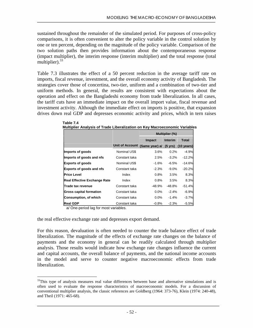
MODELING THE MACRO-ECONOMY OF BANGLADESHA
sustained throughout the remainder of the simulated period. For purposes of cross-policy comparisons, it is often convenient to alter the policy variable in the control solution by one or ten percent, depending on the magnitude of the policy variable. Comparison of the two solution paths then provides information about the contemporaneous response (impact multiplier), the interim response (interim multiplier) and the total response (total multiplier).33
Table 7.3 illustrates the effect of a 50 percent reduction in the average tariff rate on imports, fiscal revenue, investment, and the overall economy activity of Bangladesh. The strategies cover those of concertina, two-tier, uniform and a combination of two-tier and uniform methods. In general, the results are consistent with expectations about the operation and effect on the Bangladeshi economy from trade liberalization. In all cases, the tariff cuts have an immediate impact on the overall import value, fiscal revenue and investment activity. Although the immediate effect on imports is positive, that expansion drives down real GDP and depresses economic activity and prices, which in tern raises
the real effective exchange rate and depresses export demand.
Table 7.4 Multiplier Analysis of Trade Liberalization on Key Macroeconomic Variables
Multiplier (%)
Impact Interim Total Unit of Account (Same year) a/ (5 yrs) (10 years) Imports of goods Nominal US$ 3.6% 0.2% -4.9%
Imports of goods and nfs Constant taka 2.5% -3.2% -12.2%
Exports of goods Nominal US$ -1.6% -6.5% -14.6%
Exports of goods and nfs Constant taka -2.3% -9.0% -20.2%
Price Level Index 0.8% 3.5% 8.3%
Real Effective Exchange Rate Index 0.8% 3.5% 8.3%
Trade tax revenue Constant taka -48.9% -48.8% -51.4%
Gross capital formation Constant taka 0.0% -2.4% -6.9%
Consumption, of which Constant taka 0.0% -1.4% -3.7%
Real GDP Constant taka -0.8% -2.3% -5.5% a/ One-period lag for most variables.
For this reason, devaluation is often needed to counter the trade balance effect of trade liberalization. The magnitude of the effects of exchange rate changes on the balance of payments and the economy in general can be readily calculated through multiplier analysis. Those results would indicate how exchange rate changes influence the current and capital accounts, the overall balance of payments, and the national income accounts in the model and serve to counter negative macroeconomic effects from trade liberalization. 33This type of analysis measures real value differences between base and alternative simulations and is often used to evaluate the response characteristics of macroeconomic models. For a discussion of conventional multiplier analysis, the classic references are Goldberg (1964: 373-76), Klein (1974: 240-48), and Theil (1971: 465-68).
- 52 -

MODELING THE MACRO-ECONOMY OF BANGLADESHA
Chapter 8: Summary and Conclusions The present model provides a parsimonious representation of the macro economy of Bangladesh. It aims to serve a dual purpose. First, it provides a framework for making rational and consistent predictions about Bangladesh's overall economic activity, the standard components of the balance of payments, the expenditure concepts of the national accounts, and the financial sector balances. Secondly, it offers a means of quantitatively evaluating the impact of alternative policy reforms on the economy, and assessing the feedback effects that changes in key macroeconomic variables of the economy produce in other sectors. These two objectives are closely related since the capacity to make successful predictions depends on the model's ability to capture the interrelationships of the real and financial components of the economy. The modeling procedure described in this study has sought to account for the structure of the Bangladesh economy, the availability of data, and the degree of stability of time-series estimates of parameters. The nature of the modeling process of the Bangladeshi economy has motivated the design of a system that can grow and evolve with the economy. The present version of the model incorporates both the real and financial sectors of the economy within the existing exchange rate system. The objective is to provide a mechanism to link policies and targets while, at the same time, providing an easy and adaptable means of both forecasting key macroeconomic variables and simulating the interrelationships between economic policy initiatives. The present form of the model therefore provides a representation of the economy of Bangladesh that allows for considerable flexibility in its usage for forecasting, selection of the policy mix and instruments for the targets of a program, and determination of the appropriate sequencing of policy changes. The model applies a conventional IS-LM framework to the economic system and, as a policy-oriented system, it incorporates key parameters for policy formulation. At the onset, the model is designed as a parsimonious representation of the underlying data generating system for key behavior relationships. The conceptual approach to the present model is based on conventional economic theory, although the empirical specification of the conventional theory is not well established since there are numerous approaches to the specification, estimation and testing procedures in standard macro models. The parsimonious nature of the model makes it tractable from an operational point of view, and it provides the basis for subsequent extensions of the public and financial sectors, as well as the domestic and external sectors of the economy.
- 53 -

MODELING THE MACRO-ECONOMY OF BANGLADESHA
Annex: Model Listing in Eviews '_________________________________________________________ 'MACROECONOMIC MODEL OF BANGLADESH 'January 2002 '_________________________________________________________ 'Preliminaries: 'Assign statement to put all simulated variables into variables ending with _f: assign @all _f 'Trace solution for key variables '@trace NYBDR '------------------------------- 'MODEL ASSUMPTIONS '------------------------------- 'Note: Value = 1.00 means no change; value < 1 indicates a decline; value > 1 an increase. 'Enter assumptions about the following rates: '(1) Percent Changes in Nominal Exchange Rate of Bangladesh: 'nebd = 1.04 'or enter year-by-year data in series EXBDD '(2) Percent Changes in Nominal Cross-Rate Exchange Rate Indices of Bangladesh with (a) North America (crna), (b) European Union (creu), and (c) Asia (cras): crna = 1.02 creu = 1.02 cras = 1.02 '(3) Inflation of (a) North America (crna), (b) European Union (creu), and (c) Asia (cras): gpna = 1.02 gpeu = 1.02 gpas = 1.02 '(4) Percentage Change in World Trade Prices of Imported products: gpmv = 1.02 '(5) Percentage Change in World Trade Prices of Exported products: gpcm = 1.01 '(6) Percentage Change in Real GDP of World: 'gywd = 1.03 'or enter year-by-year data in series LYWDR '(7) BOP: Percentage Change in income receipts from factor services: g1 = 1.04 '(8) BOP: Percentage Change in income payments for factor services: g2 = 1.04 '(9) BOP: Percentage Change in Government Transfers: g3 = 1.0
- 54 -

MODELING THE MACRO-ECONOMY OF BANGLADESHA
'(10) BOP: Percentage Change in Private Transfers: g4 = 1.0 '(11) BOP: Percentage Change in Capital Account: g5 = 1.0 '(12) BOP: Percentage Change in FDI: g6 = 1.0 '(13) BOP: Percentage Change in Portfolio Investment g7 = 1.0 '(14) BOP: Percentage Change in Other Investment: g8 = 1.0 '(15) BOP: Errors and Omissions (million US$) er1 = -720 '(16) GOV: Average trade tax rate: ttr = 0.1957 '(17) GOV: Percentage Change in Non-tax revenue g9 = 1.04 '(18) GOV: Percentage Change in Current expenditures g10 = 1.04 '(19) GOV: Percentage Change in Food Account Surplus g11 = 1.0 '(20) GOV: Percentage Change in Annual Development Program g12 = 1.0 '(21) GOV: Percentage Change in Non ADP-Capital and Net Lending g13 = 1.0 '(22) NIA: Growth rate of Government Investment g14 = 1.04 '(23) NIA: Statistical Discrepancy er2 = 19846.49 '(24) NIA: Net Factor Income from Abroad: g15 = 1.0 '(25) NIA: Net Current Transfer from Abroad: g16 = 1.0 '(26) MONEY: Net Foreign Assets: g17 = 1.0 '(27) MONEY: Other Net Domestic Assets g18 = 1.12
- 55 -
MODELING THE MACRO-ECONOMY OF BANGLADESHA
'-------------------------------------------- 'PRICES AND EXCHANGE RATES '-------------------------------------------- 'GDP Deflator and Inflation of Bangladesh: '----------------------------------------------------------- :EQ_PRICE '(Calculates NCPIP) NYBDP = NYBDP(-1) * NCPIP/NCPIP(-1) NINFP = (NYBDP/NYBDP(-1) - 1)*100 'CPI of US and Deflators of Trading Partners: '--------------------------------------------------------------- NYNAP = NYNAP(-1) * gpna USPIP = USPIP(-1) * gpna NYEUP = NYEUP(-1) * gpeu NYASP = NYASP(-1) * gpas 'Nominal Exchange Rate of Bangladesh: '-------------------------------------------------------- 'EXBDD = EXBDD(-1) * nebd 'Nominal Cross-Rate Indices of Bangladesh: '------------------------------------------------------------- EXNA96 = EXNA96(-1) * crna EXEU96 = EXEU96(-1) * creu EXAS96 = EXAS96(-1) * cras 'Real Cross-Rate Indices of Bangladesh: '---------------------------------------------------------- EXNAR = (1/EXNA96) * (NCPIP/ NYNAP) * 10000 EXEUR = (1/EXEU96) * (NCPIP/ NYEUP) * 10000 EXASR = (1/EXAS96) * (NCPIP/ NYASP) * 10000 'Real Exchange Rates of Bangladesh: '---------------------------------------------------- EXBDR = EXNAR * 0.477423 + EXEUR * 0.461656 + EXASR * 0.060921 '=========================== 'BALANCE OF PAYMENTS BLOCK '=========================== 'Global Economy Determinants: '-------------------------------------------- '(1) World GDP 'LYWDR = LYWDR(-1) * gywd '(2) World Prices of Manufactures PCOM = PCOM(-1) * gpcm '(3) Export Determinant 2: World Primary Commodity Prices PMUV = PMUV(-1) * gpmv '---------------------- 'Current Account '----------------------
- 56 -

MODELING THE MACRO-ECONOMY OF BANGLADESHA
'Export Volume of Goods: :EQ_XQ '(Solves for XMEQR) 'Export Price of Goods: XMEPI = XMEPI(-1) * PCOM/PCOM(-1) 'Export Value of Goods: XMEVD = XMEQR * (XMEPI /100) * XSTFALL0102 'Import Volume of Goods: :EQ_ZQ '(Solves for MMEQR) 'Import Price of Goods: MMEPI = MMEPI(-1) * (PMUV / PMUV(-1)) 'Import Value of Goods: MMEVD = -MMEQR * (MMEPI /100) * MSTFALL0102 'Non-Factor Services: '(1) Service receipts - :EQ_XS '(Solves for CSRED) '(2) Service payments - :EQ_ZS '(Solves for CSPYD) 'Income: CYRED = CYRED(-1) * g1 CYPYD = CYPYD(-1) * g2 'Transfers: CTGVD = CTGVD(-1) * g3 CTPRD = CTPRD(-1) * g4 'Balances in Current Account: '------------------------------------------ '(a) Trade balance, dollar value: CTBLD = XMEVD + MMEVD '(b) Net services, dollar value: CSBLD = CSRED + CSPYD '(c) Exports of Goods and Non-Factor Services: CXGSD = XMEVD + CSRED '(d) Imports of Goods and Non-Factor Services: CMGSD = MMEVD + CSPYD '(e) Net income: CYBLD = CYRED + CYPYD '(d) Net transfers: CTRBD = CTGVD + CTPRD
- 57 -

MODELING THE MACRO-ECONOMY OF BANGLADESHA
'(e) Current account balance, dollar value: CACBD = CTBLD + CSBLD + CYBLD+ CTRBD '--------------------- 'Capital Account '--------------------- KCABD = KCABD(-1) * g5 '------------------------- 'Financial Account '------------------------- 'Foreign Direct Investment (FDI): KFDID = KFDID(-1) * g6 'Portfolio Investment: KPRLD = KPRLD(-1) * g7 'Other Investment: KOIND = KOIND(-1) * g8 'Balance on Financial Account: KFIND = KFDID + KPRLD + KOIND 'Errors and Omission: NERRD = er1 'Overall Balance, Financing, and Debt '(a) Overall balance of balance of payments, dollar value: BOPBD = CACBD + KCABD + KFIND + NERRD '=================== 'GOVERNMENT BUDGET '=================== '------------------- 'A. REVENUE '------------------- 'Tax on trade: '------------------- NGTTR = ttr * (-MMEVD/(USPIP/100) * EXBDD) 'Other revenue '--------------------- ':EQ_TAXOTH NGTOR = NGTOR(-1) 'Total tax revenue '-------------------------- NGTXR = NGTOR + NGTTR 'Non-tax revenue '------------------------ NGNTR = NGNTR(-1) * g9 'Total revenue
- 58 -

MODELING THE MACRO-ECONOMY OF BANGLADESHA
'-------------------- NGTRR = NGTXR + NGNTR '---------------------------- 'B. EXPENDITURES '---------------------------- 'Current expenditures '------------------------------ NGCER = NGCER(-1) * g10 'Food Account Surplus '-------------------------------- NGIPR = NGIPR(-1) * g11 'Annual Development Program '------------------------------------------- NGOER = NGOER(-1) * g12 'Non ADP-Capital and Net Lending '------------------------------------------------- NGCPR = NGCPR(-1) * g13 'Total expenditures '--------------------------- NGTER = NGCER + NGIPR + NGOER + NGCPR 'Residual '------------- GNRSR = GNRSR(-1) 'Overall balance '---------------------- NGBOR = NGTRR + NGTER + GNRSR 'Overall Balance as a Percent of GDP: '----------------------------------------------------- govdef = NGBOR/NYBDR '========================== 'NATIONAL INCOME ACCOUNTS '========================== '----------------------- 'CONSUMPTION '----------------------- 'Private Consumption: '------------------------------- :EQ_CON_PRI '(solves for NCPRR) 'Government Consumption: '-------------------------------------- NCGVR = NCGVR(-1) * NGCER/ NGCER(-1) 'Total Consumption '---------------------------
- 59 -

MODELING THE MACRO-ECONOMY OF BANGLADESHA
NCTTR=NCGVR + NCPRR '------------------- 'INVESTMENT '------------------- 'Private '---------- :EQ_INV_PRI '(solves for NIPRR) 'Public '--------- NIGVR = NIGVR(-1) * g14 'Investment Total '------------------------ NITTR = NIPRR + NIGVR 'Domestic Demand '--------------------------- NCIDR = NCTTR + NITTR 'Exports of goods and NFS: '-------------------------------------- CXGSR=CXGSR(-1)*((CXGSD*EXBDD)/(NYBDP/100))/((CXGSD(-1)*EXBDD(-1))/(NYBDP(-1)/100)) 'Imports of goods and NFS: '-------------------------------------- CMGSR=CMGSR(-1)*((CMGSD*EXBDD)/(NYBDP/100))/((CMGSD(-1)*EXBDD(-1))/(NYBDP(-1)/100)) 'Balance on Goods and NFS '---------------------------------------- CBGSR = CXGSR - CMGSR '----------------------------------- 'GDP BY EXPENDITURES '----------------------------------- NTBDR = CBGSR + NITTR + NCTTR 'Statistical Discrepancy '--------------------------------- NYSDR = er2 'GDP at Market Prices '------------------------------- NYBDR = NTBDR + er2 'Net Factor Income from Abroad '--------------------------------------------- NNFYR = NNFYR(-1) * g15 'Gross National Income at Market Prices '--------------------------------------------------------- NGNYR = NYBDR + NNFYR
- 60 -

MODELING THE MACRO-ECONOMY OF BANGLADESHA
'Net Current Transfer from abroad '------------------------------------------------ NNCTR = NNCTR(-1) * g16 'Gross Disposable National Income '-------------------------------------------------- NDNYR = NGNYR + NNCTR 'Gross Domestic Savings '------------------------------------ NGDSR = NYBDR - NCTTR 'Gross National Savings '------------------------------------- NGNSR = NDNYR - NCTTR 'Current Account Balance '------------------------------------ CACBR = NGNSR - NITTR - NYSDR '============= 'GDP BY ORIGIN '============= 'Value added of primary sector '----------------------------------------------- :EQ_YA '(solves for NVA1R) 'Value added of tertiary sector '-------------------------------------------- :EQ_YC '(solves for NVA3R) 'Value added of secondary sector '----------------------------------------------- NVA2R = NVATR - NVA1R - NVA3R 'Trade Taxes '------------------ NVTTR = NVTTR(-1) * NGTTR/NGTTR(-1) 'Total Value Added '-------------------------- NVATR = NYBDR - NVTTR '================= 'MONETARY SECTOR '================= 'Net Foreign Assets: '---------------------------- FNFAL = FNFAL(-1) * g17 'Net Domestic Assets: Monetarization of Fiscal Deficit:
- 61 -
MODELING THE MACRO-ECONOMY OF BANGLADESHA
'-------------------------------------------------------------------------- FNDGL = - NGBOR* NYBDP/100 'Net Domestic Assets: Other: '---------------------------------------- FNDOL = FNDOL(-1) * g18 'Net domestic assets '----------------------------- FNDAL = FNDGL + FNDOL 'Total liquidity: '----------------------------- FNTLL = FNFAL + FNDAL 'M2, Nominal '------------------ FM2VL = FNTLL 'M2, Real '------------------ FM2VR = FM2VL/(NCPIP/100) 'Interest rate, nominal '------------------------------- VIBON = VIBOR(-1) + (NINFP * 100) VIBOR = VIBON - (NINFP * 100) '================= 'POVERTY ESTIMATES '================= 'Rural Per Capita Income Index (1992=100) '------------------------------------------------------------- NYRPR = NYRPR(-1) * (1 + P_NVA1R - 0.0099) 'Urban Per Capita Income Index (1992=100) '------------------------------------------------------------- NYUPR = NYUPR(-1) * (1 + (P_NVA2R+P_NVA3R)/2 - 0.0315) '%Change in Rural PC Income from 2000 Base '------------------------------------------------------------------- P_NYRPR = (NYRPR-100)/100 '%Change in Urban PC Income from 2000 Base '------------------------------------------------------------------- P_NYUPR = (NYUPR-100)/100 '%Change in Rural Headcount Index '--------------------------------------------------- P_HCR = P_NYRPR * -0.82 '%Change in Urban Headcount Index '---------------------------------------------------- P_HCU = P_NYUPR * -1.09
- 62 -

MODELING THE MACRO-ECONOMY OF BANGLADESHA
'Rural Headcount Index '--------------------------------- HCR = 53.0 * (1+P_HCR) 'Urban Headcount Index '---------------------------------- HCU = 36.6 * (1+P_HCU) 'National Headcount Index '------------------------------------- HCN = HCR * 0.82 + HCU * 0.18 '======= 'RATIOS '======= 'Investment/GDP '------------------------ R_INVEST = NITTR/NYBDR '==================== 'PERCENTAGE CHANGES '==================== '----------------------------------------------- 'PRICES AND EXCHANGE RATES '----------------------------------------------- 'Nominal Exchange Rate, Tk/US$: P_EXBDD = @pch(EXBDD) 'Inflation P_NCPIP = @pch(NCPIP) 'Real Exchange Rate, FY96=100: P_EXBDR = @pch(EXBDR) '-------------------------------------------------------- 'BALANCE OF PAYMENTS (Million US$) '-------------------------------------------------------- 'Merchandise Import Value, US$: P_MMEVD = @pch(MMEVD) 'Merchandise Export Value, US$: P_XMEVD = @pch(XMEVD) 'Non-Factor Service Receipts, US$: P_CSRED = @pch(CSRED) 'Non-Factor Service Payments, US$: P_CSPYD = @pch(CSPYD) 'Exports of Goods and NFS (Mill US$) p_CXGSD = @pch(CXGSD)
- 63 -

MODELING THE MACRO-ECONOMY OF BANGLADESHA
'Imports of Goods and NFS (Mill US$) p_CMGSD = @pch(CMGSD) 'Foreign Direct Investment (Mill US$) P_KFDiD = @pch(KFDID) 'Overall Balance of Payments, mill.US$: BOPBD = BOPBD '------------------------------------------------------------------ 'NATIONAL INCOME ACCTS (Constant FY96Tk) '------------------------------------------------------------------ 'Exports of goods and nfs: P_CXGSR = @pch(CXGSR) 'Imports of goods and nfs: P_CMGSR = @pch(CMGSR) 'Private Consumption: P_NCPRR = @pch(NCPRR) 'Government Consumption: P_NCGVR = @pch(NCGVR) 'Total Consumption: P_NCTTR = @pch(NCTTR) 'Private Investment: P_NIPRR = @pch(NIPRR) 'Public Investment: P_NIGVR = @pch(NIGVR) 'Total Investment: P_NITTR = @pch(NITTR) 'Gross Domestic Product: P_NYBDR = @pch(NYBDR) 'Gross National Income: P_NGNYR = @pch(NGNYR) 'Gross Disposable National Income: P_NDNYR = @pch(NDNYR) 'Gross Domestic Savings: P_NYDSR = @pch(NGDSR) 'Gross National Savings: P_NGNSR = @pch(NGNSR) 'Current Account Balance: P_CACBR = @pch(CACBR) '----------------------
- 64 -

MODELING THE MACRO-ECONOMY OF BANGLADESHA
'GDP by Origin '---------------------- 'Primary Sector P_NVA1R=@pch(NVA1R) 'Secondary Sector P_NVA2R=@pch(NVA2R) 'Tertiary Sector P_NVA3R=@pch(NVA3R) '------------------------------- 'MONETARY SURVEY '------------------------------- 'Net Foreign Assets: P_FNFAL=@pch(FNFAL) 'Net Domestic Assets: P_FNDAL=@pch(FNDAL) 'Monetarization of Fiscal Deficit: P_FNDGL=@pch(FNDGL) 'M2, Broad Money: P_FM2VL=@PCH(FM2VL) 'M2, Real: P_FM2VR=@PCH(FM2VR) '------------------------------------ 'GOVERNMENT BUDGET '------------------------------------ 'Tax on Trade: P_NGTTR=@PCH(NGTTR) 'Implicit Trade Tax Rate: ttr = ttr 'Other Taxes: P_NGTOR=@PCH(NGTOR) 'Current Expenditures: P_NGCER=@PCH(NGCER) 'Total Expenditures: P_NGTER=@PCH(NGTER) 'Share of Trade Taxes in Total Tax Revenue S_TD_TX = NGTTR/NGTXR 'Fiscal Deficit: govdef = NGBOR/NYBDR
- 65 -

MODELING THE MACRO-ECONOMY OF BANGLADESHA
Bibliography and References
Andrews, D.W.K. (1993), "Tests for Parameter Instability and Structural Change with Unknown
Change Point", Econometrica, 61(4) 821-56. Argy, V. (1994), International Macroeconomics: Theory and Policy. London: Routledge. Asian Development Bank (1991), "Economic Review and Bank Operations Paper (ERBOT) -
Bangladesh: 1991". Attachment to Board Paper. Asian Development Bank (1992), "Economic Review and Bank Operations Paper (ERBOT) -
Bangladesh: 1992". Attachment to Board Paper. Asian Development Bank (2000), Country Economic Review: Bangladesh. Economic Unit.
Bangladesh Resident Mission. Asian Development Bank (2001), Quarterly Economic Update Bangladesh. Economic Unit.
Bangladesh Resident Mission. Banerjee, A., J. Dolado, J.W. Galbraith, and D.F. Hendry (1993), Cointegration, Error-
Correction, and the Econometric Analysis of Non-Stationary Data. Oxford: Oxford University Press.
Barro, R.J. (1997), Macroeconomics. (Fifth edition). Cambridge, Mass: The MIT Press. Blanchard, O.B. and S. Fischer (1996), Lectures in Macroeconomics. Cambridge, Mass: The
MIT Press. Bluhosch, B., A Freytag, and M. Kruger (1996), International Competitiveness and the Balance
of Payments: Do Currency Account Deficit and Surpluses Matter? Cheltenham, UK: Edward Elgar Publishing Ltd.
Bowen, H.P., A. Hollander, and J-M Viaene (1998), Applied International Trade Analysis.
Michigan University Press. Chen, S. and M. Ravallion (2000), “How Did the World’s Poorest Fare in the 1990s?” World
Bank. Policy Research Working Paper 2409.
Cole, I.M. (1992), “Fiscal Dependence on Trade Taxes and Economic Development: Additional Results and a Reconciliation of the Empirical Evidence”. Applied Economics 24.
- 66 -

MODELING THE MACRO-ECONOMY OF BANGLADESHA
Cole, I.M. (1993), “Fiscal Dependence on Trade Taxes and the Level of Economic
Development: A Reply”. Applied Economics 25. Corden, M. (1985), Inflation, Exchange Rates and the World Economy. (Third edition). Oxford:
Clarendon Press. Corden, M. (1990), “Macroeconomic Adjustment in Developing Countries”. World Bank
Research Observer 4(1): 51-64. Davidson, J., et al. (1978), “Cointegration in Recursive Systems: The Structure of Wage and
Price Determination in the United Kingdom”. London School of Economics Econometrics Programme Discussion Paper.
Dutta, D. and N. Ahmed (undated), “An Aggregate Import Demand Function for Bangladesh: A
Cointegration Approach”. Department of Economics, University of Sydney. Easterly, W. (1989), "A Consistency Framework for Macroeconomic Analysis". PRE Working
Paper 234. Washington, DC: International Bank for Reconstruction and Development. Easterly, W., E.C. Hwa, P. Kongsamut, and J. Zizek (1990), "Modeling the Macroeconomic
Requirements of Policy Reform". PRE Working Paper, No. 417. Washington, DC: International Bank for Reconstruction and Development.
Edwards, S. (1988), Exchange Rate Misalignment in Developing Countries. Baltimore: Johns
Hopkins University Press. Engle, R.F., and C.W.J. Granger (1987), "Co-Integration and Error Correction: Representation,
Estimation, and Testing". Econometrica, 55(2): 251-76. Fry, M.J. (1995), Money, Interest and Banking in Economic Development. Baltimore, Md: The
Johns Hopkins University Press. Jha, R. (1994), Macroeconomics for Developing Countries. London: Routledge. Gallup, J.L., S. Radelet, and a. Warner (1998), “Economic Growth and Income of the Poor”.
Cambridge, Mass.: Harvard Institute for International Development.
Goldstein, M. and M.S. Khan (1985), “Income and Price Effects in Foreign Trade”. In R.W. Jones and P.B. Kenen (eds), Handbook of International Economics, 2. Amsterdam: North-Holland.
Greenaway, D. (1984), “A Statistical Analysis of Fiscal Dependence on Trade Taxes and
Economic Development”. Public Finance 39(1). Greenaway, D., and C. Milner (1991), “Fiscal Dependence on Trade and Trade Policy Reform”.
Journal of Development Studies 27.
- 67 -

MODELING THE MACRO-ECONOMY OF BANGLADESHA
Greenaway, D., and D. Sapsford (1987), “Further Econometric analysis of the Relationship
between Fiscal Dependence on Trade Taxes and Economic Development”. Pubic Finance 42(2).
Hallwood, C.P., and R. MacDonald (1994), International Money and Finance. Oxford:
Blackwell. Harvey, A.C. (1991), The Econometric Analysis of Time Series. Cambridge, Mass.: MIT Press. Hendry, D.F. (1988), "The Encompassing Implications of Feedback versus Feedforward
Mechanisms in Econometrics." Oxford Economic Papers, 40, 132-139. Hendry, D.F., A.R. Pagan, and J.D. Sargan (1984), “Dynamic Specification”. In Z. Griliches and
M.D. Intriligator (eds), Handbook of Econometrics, Vol. 2-3. Amsterdam: North-Holland.
Hood, R. (1998), “Fiscal Implications of Trade Reform”. In J. Nash and W. Takacs (eds.), Trade
Policy Reform: Lessons and Implications . Washington, DC: International Bank for Reconstruction and Development.
Intriligator, M.D., R.G. Bodkin, and C. Hsiao (1996), Econometric Models, Techniques and
Applications. (Second edition). Upper Saddle River, NJ: Prentice Hall. Isard, P., and H. Faruqee (1998), "Exchange Rate assessment: Extensions of the Macroeconomic
Balance Approach". Occasional Paper 167. Washington, DC: International Monetary Fund.
Kakwani, N., and E. Pernia (2000), “What is Pro-poor Growth”. Asian Development Review 18. Klein, L.R. (1974), A Textbook of Econometrics. Englewood Cliffs, NJ: Prentice-Hall. Krugman, P.R., and M. Obstfeld (1997), International Economics: Theory and Policy. (Fourth
edition). Reading, Mass: Addision-Wesley. Leamer, E. and R.M. Stern (1970), Quantitative International Economics. Boston: Allyn and
Bacon. Lord, M.J. (1991a), Imperfect Competition and International Commodity Trade: Theory,
Dynamics, and Policy Modelling. Oxford: Clarendon Press. Lord, M.J. (1991b), "Price Formation in Commodity Markets." Journal of Applied
Econometrics, Vol.6: 239-254.
- 68 -

MODELING THE MACRO-ECONOMY OF BANGLADESHA
Lord, M.J. (1993), A Macroeconomic Model under Fixed Exchange Rates for Romania.
National Commission for Economic Forecasting of the Council for Coordination, Strategy, and Economic Reform of the Government of Romania.
Lord, M.J., P.G. Christopher, S.M. Lewarne (1995), A Macroeconomic Model for Kazakhstan: A
Policy-Oriented Framework and Preliminary Results. Prepared for USAID/Almaty by Boye-Lord International Ltd and the Office of Monetary Policy Research, National Bank of Kazakhstan.
Lord, M.J. (1998),a “Modeling the Open Macro-Economy of Viet Nam”. Prepared for the State
Bank of Viet Nam and Asian Development Bank. Lord, M.J., ed. (1998b), The Handbook of Latin American Trade in Manufactures. Gheltenham,
Glos.: Edward Elgar Publishing Ltd. Lord, M.J. (1999), “The Elasticities Approach to Egypt’s Balance of Payments and Equilibrium
Exchange Rate”. Cairo: Development Economic Policy Reform Analysis Project (DEPRA), Ministry of Economy and Trade.
Lord, M.J. (2001), Macroeconomic Policies for Poverty Reduction in Cambodia. Prepared for
the Asian Development Bank. Lucas, R. (1976), “Econometric Policy Evaluations: A Critique”. Carnegie Rochester
Conference Series on Public Policy. No. 1. Lundberg, M., and L. Squire (2000), “Inequality and Growth: Lessons for Policy”. Washington,
DC: The World Bank, Global Development Network.
Mohan, G., et al. (2000), Structural Adjustment: Theory, Practice and Impacts. London: Routledge.
Mankiw, N.G. (1997), Macroeconomics (Third edition). New York, N.Y.: Worth Publishing. Mitra, P. (1992), “The Coordinated Reform of Tariffs and Indirect Taxes”. World Bank Research
Observer 7(2). Muriende, V. (1993), Macroeconomic Policy Modellling for Developing Countries. Aldershot:
Avebury. Obstfeld, M. and K. Rogoff (1998), Foundations of International Macroeconomics. Cambridge,
Mass: The MIT Press. Pindyck, R.S, and D.L. Rubinfeld (1998), Econometric Models and Economic Forecasts.
Boston: McGraw-Hill.
- 69 -

MODELING THE MACRO-ECONOMY OF BANGLADESHA
Pritchett, L., and G. Sethi (1994), “Tariff Rates, Tariff Revenue, and Tariff Reform: Some New
Facts”. The World Bank Economic Review 8(1). Rati, R. (1994), “Level of Economic Development and Share of Trade Taxes in government
Revenue: Some Evidence from Individual-Country Time-Series Data”. Public Finance 49(3).
Romer, D. (1996), Advanced Macroeconomics. New York: McGraw-Hill Companies, Inc. Sachs and Larrain (1993), Macroeconomics in the Global Economy. Englewood Cliffs, New
Jersey: Prentice Hall. Theil, H. (1971), Principles of Econometrics. New York: John Wiley. Tokarick, S. (1995), “External Shocks, the real Exchange Rate, and Tax Policy”. IMF Staff
Papers 42(1). Vito, T. (1989), “The Impact of Macroeconomic Policies on the Level of Taxation and the Fiscal
Balance in Developing Countries”. IMF Staff Papers 36(3). Wong, C.-H. and L. Carranza (1998), “Policy Responses to External Imbalances in Emerging
Market Economies-Further Empirical Results”. Washington, DC: IMF Working Paper WP/98/103.
- 70 -