Dynamic capital structure with callable debt and debt renegotiations

Journal of Corporate Finance 29 (2014) 644–661

Contents lists available at ScienceDirect

Journal of Corporate Finance

j ourna l homepage: www.e lsev ie r .com/ locate / jcorpf in

Dynamic capital structure with callable debt anddebt renegotiations

Peter Ove Christensen a, Christian Riis Flor b, David Lando c,⁎, Kristian R. Miltersen c

a Dept. of Economics and Business, Aarhus University, Fuglesangs Allé 4, 8210 Aarhus V, Denmarkb Dept. of Business and Economics, University of Southern Denmark, Campusvej 55, 5230 Odense M, Denmarkc Dept. of Finance, Copenhagen Business School, Solbjerg Plads 3, 2000 Frederiksberg, Denmark

a r t i c l e i n f o

⁎ Corresponding author. Tel.: +45 3815 3613.E-mail addresses: [email protected] (P.O. C

0929-1199/$ – see front matter © 2013 Published byhttp://dx.doi.org/10.1016/j.jcorpfin.2013.09.001

a b s t r a c t

Article history:Received 28 September 2012Received in revised form 9 July 2013Accepted 1 September 2013Available online 10 September 2013

We consider a dynamic trade-off model of a firm's capital structure with debt renegotiation.Debt holders only accept restructuring offers from equity holders backed by threats which arein the equity holders' own interest to execute. Our model shows that in a completeinformation model in which taxes and bankruptcy costs are the only frictions, violations of theabsolute priority rule (APR) are typically optimal. The size of the bankruptcy costs and theequity holders' bargaining power affect the size of APR violations, but they have only a minorimpact on the choice of capital structure.

© 2013 Published by Elsevier B.V.

JEL classification:G32G33G13

Keywords:Dynamic capital structureDebt restructuringViolation of absolute priority

1. Introduction

Empirical evidence suggests that for most firms in financial distress, debt and equity holders agree—either voluntarily or aspart of a Chapter 11 process—to restructure the firm's capital thereby allowing the firm to continue operation, see Weiss (1990),Gilson et al. (1990), and Morse and Shaw (1988). We consider a dynamic capital structure model in which the going concernvalue of the firm makes debt renegotiation optimal for debt and equity holders. If the firm is in financial distress, the equityholders can make a take-it-or-leave-it offer to the existing debt holders in order to reestablish an optimal capital structure for thefirm. The debt holders always have the option to reject the offer, but their decision whether to accept or reject depends on whatthey anticipate will happen if they reject. A critical feature of our model is that debt holders do not accept offers from equityholders which are not credible. An example of a non-credible threat is if equity holders threaten to liquidate the firm even if itwould be better for them to keep servicing the existing debt. In equilibrium, the equity holders only make renegotiation offerswhich are accepted by the debt holders, but the off-the-equilibrium-path rejection values of debt and equity are the key indetermining the equilibrium offer. We find that debt holders rationally accept deviations from the absolute priority rule as theoutcome of the renegotiation game. The intuition is that equity holders know that non-credible threats will be rejected by debtholders and, hence, equity holders postpone their renegotiation offer to the point at which liquidation becomes a credible threat.At this point it is rational for the debt holders to accept deviations from the absolute priority rule, since liquidation is thealternative.

hristensen), [email protected] (C.R. Flor), [email protected] (D. Lando), [email protected] (K.R. Miltersen).

Elsevier B.V.

http://crossmark.crossref.org/dialog/?doi=10.1016/j.jcorpfin.2013.09.001&domain=pdf

http://dx.doi.org/10.1016/j.jcorpfin.2013.09.001

mailto:[email protected]




http://dx.doi.org/10.1016/j.jcorpfin.2013.09.001

http://www.sciencedirect.com/science/journal/09291199

645P.O. Christensen et al. / Journal of Corporate Finance 29 (2014) 644–661

We also allow for callable debt and reissuance of debt when the firm does well and, hence, our model extends and unifiesseveral strands of the literature on dynamic capital structure. Compared to existing models, the combination of renegotiation andcallability significantly increases the tax advantage to debt.

We consider a firm with a simple capital structure consisting of equity and a single class of callable perpetual debt.Following Goldstein et al. (2001), we use the firm's earnings before interest and taxes (EBIT) as the driving state variable.For an initial level of EBIT, an optimal capital structure is chosen to maximize firm value by trading off the tax advantageto debt, the cost of financial distress, and future restructuring costs. Subsequent to the issuance of debt and equity, theequity holders continuously decide whether to continue servicing the existing debt or to restructure the firm's capital. Asthe firm's EBIT increases, equity holders prefer more debt to better exploit the tax shield. As the firm's EBIT decreases, theequity holders prefer less debt in order to reduce the cost of financial distress. The initial values of debt and equityrationally reflect the equity holders' ex-post incentives to restructure as well as the payoffs received if restructuringoccurs.

For reasons that will be explained when we define our model, we solve for debt and equity values in a case where there arefinitely many renegotiation options. The starting point is first to solve a case with no renegotiation possibility at the lowerboundary. This benchmark case is comparable to Goldstein et al. (2001), and is in accordance with classical models such as Blackand Cox (1976), Merton (1974), and Leland (1994). In these models, the firm is liquidated at the lower boundary, and the taxadvantage to debt is lost permanently. Our benchmark model deviates from these models by assuming that the value of the firm'sproduction technology in liquidation is equal to the value for a new entrepreneur who can start afresh and optimally lever thefirm's assets.

With debt renegotiation, equity holders may continue to service the debt after a rejection by the debt holders. Tohandle this, we need a friction that leaves the firm in a different shape after one renegotiation round consisting of anoffer, a rejection, and a continuation of debt service. The friction is the loss of one renegotiation option, which bringsthe firm one step closer to the case with forced liquidation at the lower boundary. This friction is similar in spirit to thefinite number of sequential offers refinement of the Nash equilibria in the Rubinstein bargaining game, cf. Rubinstein(1982, 1987).

Our model shares an important feature with strategic debt service models, cf. Anderson and Sundaresan (1996), Mella-Barraland Perraudin (1997), Hege and Mella-Barral (2005), and Hackbarth et al. (2007): When liquidation is costly, the debt and equityholders have a common interest in saving the costs of bankruptcy. There are two key differences between our debt renegotiationmodel and the strategic debt service models. First, in strategic debt service models, a failed renegotiation proposal leads to aforced liquidation of the firm. They rule out the possibility that equity holders may continue servicing the debt with the existingcoupon payments, i.e., that the assumed bankruptcy threat to force concessions from the debt holders may not be a crediblethreat. In our model, we insist on credible threats which forces equity holders to postpone their restructuring offer. Second, inmost of the strategic debt service models, there is no restructuring of the firm's capital—the equity holders only bargain inorder to obtain temporary coupon relief; an exemption from this is e.g. Mella-Barral (1999). François and Morellec (2004),Galai et al. (2007), and Broadie et al. (2007) look at settings in which debt is not serviced while in Chapter 11, but the(original) coupon must be paid if the firm leaves Chapter 11. These papers incorporate important aspects of the Chapter 11code, e.g., the automatic stay, but a successful exit of Chapter 11 does not solve the underlying capital structure (financialdistress) problem. Annabi et al. (2010) consider the outcome of Chapter 11 as a non-cooperative game. They focus on thejudge's role, and the random intervention leads to a game in multiple rounds, but they do not consider the firm's optimalcapital structure.

Goldstein et al. (2001) find that their dynamic capital structure model gives lower leverage ratios than static capitalstructure models, ceteris paribus, since the firm can subsequently increase its outstanding debt, if EBIT increases sufficiently.By adding debt renegotiation to the model, we find that leverage ratios increase compared to the results of Goldstein et al.(2001). This is due to the fact that debt renegotiation reduces the negative impact of financial distress relatively to a setting inwhich liquidation is the only outcome of financial distress. The introduction of debt renegotiations increases the taxadvantage to debt by 50% relative to a dynamic capital structure model with no debt renegotiation for realistic parametervalues.

Our model gives a simple explanation of the violation of the absolute priority rule for firms in financial distress. SuchAPR violations are well documented in the empirical literature, see Weiss (1990), Eberhart et al. (1990), Betker (1995),Bris et al. (2006), and Altman and Hotchkiss (2010). In debt renegotiation models in which renegotiation proposals canbe backed by non-credible threats, it is not surprising that APR violations may occur. We show that APR violations occureven when we insist that successful renegotiation proposals must be backed by credible threats. On the equilibrium path,it is perfectly rational for the debt holders to accept a renegotiation proposal from the equity holders which leaves somevalue to the equity holders even though the debt holders do not recover their full principal. A rejection by the debtholders does not necessarily force an immediate liquidation of the firm. Equity holders may continue servicing the debtwith the promised coupon until the conditions become even worse. In equilibrium, equity holders postpone theirrenegotiation proposal to the point at which liquidation is a credible threat. We show that equity holders' bargainingpower has a significant impact on the absolute priority violations, but that it only has a minor impact on the choice ofcapital structure and on the ex-ante optimally levered firm value. Hackbarth et al. (2007) also consider anticipateddeviations from absolute priority that depend on the toughness of the bankruptcy regime, but the violations are not arational model outcome.

646 P.O. Christensen et al. / Journal of Corporate Finance 29 (2014) 644–661

In addition, our model predicts that the bankruptcy costs have almost no impact on the firm's optimal capital structurepolicy. In fact, in our model the firm is always more valuable alive than liquidated, and debt renegotiation ensures thatliquidation never occurs. Hence, bankruptcy costs only affect the off-the-equilibrium-path values of debt and equity and the sizeof the APR violations.We donot addresswhy restructurings occur in some cases and liquidation in others, as in for example Broadie etal. (2007).

As noted, our model provides a number of empirical implications. Note, however, that these empirical implications arerelevant at recapitalization points, i.e., for newly optimally levered firms. The distance between the upper and lower boundary atwhich the firm is recapitalized, however, is quite large. Therefore, the important caveat of Strebulaev (2007) applies, i.e.,cross-sectional analysis of leverage, which do not recognize that firms are away from their optimal leverage most of the time, maynot be consistent with our predictions. In our model, the initial choice of leverage is a strong predictor of future leverage, sincethat is the level of leverage to which firms readjust when they recapitalize. This is consistent with the persistence on leverageratios found in Lemmon et al. (2008).

2. The model

We consider a firm whose instantaneous earnings before interest and taxes (EBIT), ξ, follow a geometric Brownian motionunder the risk neutral pricing measure, i.e.,

1 Oththe exispriority

dξt ¼ ξtμdt þ ξtσdWt ; ð1Þ

given starting point, ξ0. The constants μ and σ are the drift and volatility of ξ, respectively, and W is a standard Brownian
with amotion. We can think of the origin of the EBIT process as the cash flow process generated by a production technology initiallyowned by an entrepreneur. The entrepreneur has the option to incorporate the firm (at a certain cost) based on the EBIT processby issuing debt and equity.
We assume that the firm can issue a single class of callable perpetual corporate debt with a fixed instantaneous coupon, C.The call feature of debt allows equity holders to better exploit the tax advantage to debt by increasing the amount ofoutstanding debt when earnings increase. This is an important feature to include in the model since it has a significant impacton optimal leverage as shown by Goldstein et al. (2001). Debt can only be increased by calling the existing debt andsubsequently issuing new debt.1 Debt is called at a premium, and there is a cost of issuing new debt which is proportional to theprincipal.

The after-tax payment received by the debt holders on outstanding debt with coupon C is (1 − τi)C, where τi is the rate ofpersonal interest taxes paid by debt holders. Interest expenses are deductible before paying corporate taxes at the rate τc. Hence,the amount available for dividends to equity holders is (1 − τc)(ξ − C). The dividend tax rate is τd so the after-tax paymentreceived by equity holders is (1 − τe)(ξ − C), where τe = τc + (1 − τc)τd. This assumes a symmetric tax refund if ξ b C. Inpractice, there is no tax refund for negative earnings, but there can be loss carry forwards. To mimic this friction, we assume theafter-tax dividend received by equity holders is equal to (1 − �τe)(ξ − C) for ξ b C, where � ∈ [0,1] is the effective tax refundused when the earnings before taxes, EBT = ξ − C, is negative.

We assume that there is a constant before tax riskless interest rate, r̂. Since interest income is taxable, the discount rate usedfor pricing under the pricing measure is the after-tax riskless rate r ¼ 1−τið Þr̂. This reflects an assumption that not only is interestincome taxed at the rate of τi, but there is also a tax subsidy at the rate of τi associated with interest expenses. Hence, in terms ofdynamic replication of contingent claims, the effective interest rate paid on the money market account used for borrowing in thereplicating portfolio is r. We assume throughout that μ b r to ensure that the cash flows generated from the EBIT process have afinite market value.

In all cases considered below, the restructuring policy is parameterized by two boundaries: the renegotiation (or bankruptcy)boundary, ξ, and the call boundary, ξ. Obviously, ξbξ0bξ. That is, when ξ reaches the lower boundary, the debt is renegotiated (orthe firm is declared bankrupt), and when ξ reaches the upper boundary, the debt is called. These boundaries will be derivedendogenously from the incentive compatibility constraints for the equity holders, and they depend on the mechanism used forrenegotiating the firm's debt at the lower boundary. As a first step in solving the model, we take the boundaries and the pay-offsat the boundaries as exogenously given.

Debt and equity are time-homogeneous claims on the EBIT process, i.e., their values do not depend on calendar time. Thepayoffs depend only on the current level of EBIT, ξt, and the level of EBIT when the debt and equity were issued, ξs, s ≤ t.Therefore, we denote the price at date t of debt and equity issued at some prior date s as D(ξt;ξs) and E(ξt;ξs), respectively.Implicitly, this means that the EBIT process {ξu}u ∈ [s,t) has stayed inside the interval ξ; ξ

� �in the time period [s,t).

erwise, the equity holders have incentives to sequentially increase the outstanding debt by issuing new debt with the same seniority, and thereby dilutingting debt. Of course, the debt holders rationally anticipate these incentives, see Leland (1994). Alternatively, new additional debt can be issued with loweras, for example, in Dockner et al. (2013) or Miltersen and Torous (2013).


We show in Appendix A that both the debt and equity price functions are positive homogeneous of degree one in (ξt,ξs) (cf.Eq. (A.6) in Appendix A). That is,

and

for an

and

where

For simthe upcoupo

and

These

2 Fisc3 The

D hξt ;hξsð Þ ¼ hD ξt ; ξsð Þ ð2Þ

E hξt ;hξsð Þ ¼ hE ξt ; ξsð Þ; ð3Þ

y ξt∈ ξ; ξh i

and h N 0. Moreover, note that this homogeneity property implies that the restructuring policy ξ; ξ� �

for eachsue of debt can be written as (dξs, uξs) for some fixed positive constants d b 1 and u N 1.
new is
Furthermore, for notational simplicity we write the initial values of debt and equity at the issue date as

D ξs; ξsð Þ ¼ ξsD 1;1ð Þ ¼ Dξs

E ξs; ξsð Þ ¼ ξsE 1;1ð Þ ¼ Eξs;

D and E are constants defined as D = D(1;1) and E = E(1;1).
whereWe define the principal of the debt issued at date s with a coupon rate c∗ξs to be the initial value of the debt Dξs (cf. Part 1 of
Conjecture 1 in Appendix A). The debt is callable at a premium, λ, at any date t ≥ s, i.e., the debt can be called (by the equityholders) at date t by paying the debt holders (1 + λ)Dξs.2 When debt is issued, there are issuance costs, k, proportional to the parvalue of the debt.3 Hence, the total proceeds to the entrepreneur at date s for issuing both perpetual debt with a coupon rate c∗ξsand equity is

A ξsð Þ ¼ E ξs; ξsð Þ þ 1−kð ÞD ξs; ξsð Þ ¼ ξs E 1;1ð Þ þ 1−kð ÞD 1;1ð Þð Þ ¼ Aξs; ð4Þ

A is a constant defined as

A ¼ E 1;1ð Þ þ 1−kð ÞD 1;1ð Þ ¼ E þ 1−kð ÞD:

plicity, assume debt is issued at date zero when the EBIT process is initiated at ξ0. We first look at boundary conditions atper boundary. When the EBIT process ξ hits uξ0, the old debt is called at a premium, λ, and new debt is issued with a highern to obtain an increased tax shield. That is, we have the following values of debt and equity at the call boundary, uξ0,

D uξ0; ξ0ð Þ ¼ 1þ λð ÞD ξ0; ξ0ð Þ¼ 1þ λð ÞDξ0

ð5Þ

E uξ0; ξ0ð Þ ¼ E uξ0;uξ0ð Þ þ 1−kð ÞD uξ0;uξ0ð Þ− 1þ λð ÞD ξ0; ξ0ð Þ¼ Au− 1þ λð ÞDð Þξ0:

ð6Þ

equations are the value-matching conditions at the upper boundary uξ0.

2.1. Liquidation at the lower boundary

The key feature of our model is the renegotiation game at the lower boundary. To be able to solve this model, we need as anintermediate step to compute the value of the firm when there is no possibility of renegotiation at the lower boundary dξ0. So thatthe debt holders' response to equity holders withholding coupons is immediate liquidation. The claim to the EBIT process is thenacquired as a going concern by a new entrepreneur who again can optimally lever the firm. A fraction, α, of the proceeds coversthe bankruptcy costs. The net proceeds go first to the debt holders to cover their original principal, and if there is a surplus, it goesto the equity holders. This is in accordance with the absolute priority rule. However, because the equity holders have limitedliability, the debt holders are in most cases not able to recover their full principal. This happens when the proceeds from the saleof assets less the bankruptcy costs are smaller than the original principal. Hence, we get the following value-matching conditionsat dξ0:

D dξ0; ξ0ð Þ ¼ min 1−αð ÞA dξ0ð Þ;D ξ0; ξ0ð Þf g¼ min 1−αð ÞAd;Df gξ0;

ð7Þ

her et al. (1989b) and Flor and Lester (2002) study the ex-ante optimal size of the call premium.se costs remove the equity holders' incentive to restructure the debt continuously when there is no call premium, i.e. when λ = 0, see footnote 1.

and

4 ThisMertonwhat ty

5 If thleave so


E dξ0; ξ0ð Þ ¼ max 1−αð ÞA dξ0ð Þ−D ξ0; ξ0ð Þ;0f g¼ max 1−αð ÞAd−D;0f gξ0:

ð8Þ

With these assumptions, we are able to price debt and equity for exogenously given boundaries by solving a fixed-pointproblem for the two unknowns E(1,1) and D(1,1).

We next take into account that the equity holders control the firm and decide (i) when to call the debt and (ii) at each instantin time whether to pay the coupons to the debt holders or not. That is, the incentives of the equity holders endogenouslydetermine the restructuring policy, and both equity and debt holders rationally anticipate these incentives already at debtissuance. The equity holders find it optimal to call the debt at uξ0 when the following condition is fulfilled:

∂∂ξ E uξ0; ξ0ð Þ ¼ A; ð9Þthe partial derivative is with respect to the first argument of the equity price function (ξ,ξ0) ↦ E(ξ,ξ0). This condition is the
where
smooth-pasting condition at the upper boundary uξ0.4

Similarly, the equity holders find it optimal to declare bankruptcy at dξ0 (by withholding the coupons) when the followingsmooth-pasting condition is fulfilled:

∂∂ξ E dξ0; ξ0ð Þ ¼ 1−αð ÞA1 1−αð ÞAd≥Df g; ð10Þ1ɛ is the indicator function for the event ɛ.
where
Given the coupon rate C = cξ0, Appendix B, shows how the value-matching and smooth-pasting conditions determine thedebt and equity price functions. In particular, for ξ = 1 we get the constants E and D. Since the optimally levered firm value, A =E + (1 − k)D, is used in the boundary conditions stated above, the derivation of the equity and debt prices (and the optimalboundaries) is actually still a fixed-point problem. Recall that E and D are determined for a given coupon rate. In order todetermine the optimally levered firm value, we must (numerically) optimize over the coupon rate c. With the optimal rate, c⁎, theoptimal capital structure policy of the firm is characterized by the constants E, D, u, d, and c⁎.

Up to this point, our model is similar to that of (Goldstein et al., 2001) but with one notable difference: (Goldstein et al., 2001)assume that the firm's assets in bankruptcy are sold off at their unlevered value, which is equal to (1 − τe)ξ/(r − μ). Hence, thedebt and equity values are known functions of ξ at the lower boundary. In our base case model, the liquidation value of the firm atthe lower boundary recognizes that the assets of the firm can subsequently be optimally levered, i.e., the tax advantage to debt isnot lost at bankruptcy. Hence, our model leads to a fixed-point problem when solving for the initial values of debt and equity dueto the optimally levered firm value both at the lower boundary and the call boundary. A similar fixed-point problem due torestructuring at the call boundary has been studied in Kane et al. (1985), Fischer et al. (1989a), and Goldstein et al. (2001).

2.2. Debt renegotiation with credible threats

The going concern value of the firm is always larger than the value after bankruptcy and, therefore, it is in the best interest ofdebt and equity holders to avoid bankruptcy at the lower boundary. While one could easily add other frictions that would makebankruptcy optimal in some cases, we focus on the outcome of debt renegotiation. In most strategic debt service models, equityholders make take-it-or-leave-it offers to the debt holders that just leave the debt holders as well off as in a bankruptcy. Hence,equity holders get the entire benefit of the saved bankruptcy costs. The problem with these debt renegotiation models is that it isnot obvious that the equity holders' threat of withholding the coupons, if the debt holders reject the restructuring proposal, is acredible threat. In fact, it almost never is in these models. If the debt holders declare the firm bankrupt, the equity holders wouldin most cases get nothing.5 Thus, if the equity holders' restructuring proposal is rejected by the debt holders, they might prefer tocontinue paying the original coupon, and thereby avoid bankruptcy.

In our model, the equity holders' proposal takes into account that acceptance by the debt holders depends on their conjectureof the equity holders' rational response to a rejection. Equity holders may decide to continue paying coupons, but nothingprevents them from immediately proposing a new restructuring. To close the model, we must introduce a friction leaving the firmin a different state after a rejected renegotiation proposal so that an identical restructuring proposal is not immediately proposed.The friction we introduce is that the equity holders are only allowed to make a finite number of renegotiation proposals. If thereare no more renegotiation options, we end up in the model of the preceding section in which the only response to equitywithholding coupons is liquidation. The finite number of renegotiation options implies that after a rejection, the firm is in adifferent shape than it was before the proposal was presented. That is, the firm has moved one step closer to a world with nopossibility of restructuring.

(or similar) smooth-pasting or high-contact conditions are used throughout the literature, see, e.g., Merton (1973); Leland (1994); Mella-Barral (1999)., footnote 60 gives an argument for the validity of this condition, but see also Dixit (1991, 1993), Brekke and Øksendal (1991, 1994) for explanations ofpe of optimality this condition leads to.e proposal is made for a very high level of EBIT it is possible that the default value of the firm is higher than the initial debt holders' principal. This wouldme value for equity holders.


The model is most easily understood in the case of one remaining renegotiation option, and we therefore consider this case indetail in what follows. For this we need additional notation. We use a subscript to denote the number of remaining options. Thus,for example, E0(1,1) now denotes the value of equity in the model of the previous subsection, i.e., the value of equity after we havetaken into account the optimal call policy and the optimal liquidation policy of the equity holders, and where the coupon has beenchosen to optimize firm value. Similarly, E0(ξ,1) denotes the value of equity when the EBIT process has moved to ξ, but the capitalstructure and policies are those determined when ξ was equal to 1.

Consider now the renegotiation game at the lower boundary, dξ0, at which the equity holders make their restructuring proposal,which is their last remaining proposal. Let E1c denote the value of equity with one remaining option based on the assumption that therestructuring proposal is rejected and that the equity holders continue to pay the original coupon c1 (which at this point is not to bethought of as chosen optimally). We can express the value of continuing with the existing coupon using the function E0 whichpresumes an optimal coupon of c0∗ . To see this, note that paying the coupon c1 would be optimal if the firm had been capitalized withzero remaining options at the starting point c1/c0∗ .6 We can therefore express the value of equity with zero remaining options andcoupon c1 as E0(dξ0, c1/c0∗), which captures the fact that equity will choose the optimal boundaries given the coupon c1, but also thatEBIT is now at dξ0. In other words, the value of equity when choosing to continue paying the existing coupon is

Sincepay ththe pr

This vdepen

In thispayme

If the

This isholderzero r

Suwith n

Hence

6 Thisdoes harenegotprincipathan ththe prin

Ec1 ¼ E0 dξ0; c1=c�0

� �:

other hand, if the restructuring proposal is rejected and the equity holders withhold the coupon payments, then the firm is
On thedeclared bankrupt (because we are then in the case with zero renegotiation options). This means that the equity value based onthe assumption that a rejection is followed by liquidation is
Eb1 ¼ max 1−αð ÞA0d−D1;0f gξ0:

the firm's going concern value in liquidation, A0, includes no options to renegotiate. The choice of whether to continue toe original coupon rate or to declare bankruptcy is in the hands of the equity holders. Hence, the equity value, assuming thatoposal leads to rejection, is the maximum of the two alternatives, i.e.,

Er1 ¼ max Ec1; Eb1

n o:

alue depends solely on values we know from solving the case with zero renegotiation options. The corresponding debt valueds on the choice of the equity holders. If the equity holders continue to pay the original coupon, the debt value is

Dc1 ¼ D0 dξ0; c1=c

�0

� �:

case, the debt holders are not in a position to force bankruptcy. On the other hand, if the equity holders cease the couponnts, the debt holders immediately declare bankruptcy. The bankruptcy value of debt is

Db1 ¼ min 1−αð ÞA0d;D1f gξ0:

debt holders reject the restructuring proposal, the value of debt is

Dr1 ¼ Dc

11 Ec1 ≥Eb1f g þ Db11 Ec1bE

b1f g:

our assumption of credible threats. Debt holders rationally anticipate whether upon a rejection it is in the interest of equitys to continue with the existing coupons or to liquidate. All values on the right hand side are available from the case withenegotiation options.ppose instead the proposal is accepted. Then the joint value of debt and equity is the optimally levered firm value, but nowo remaining options to renegotiate, i.e.,

Ea1 dξ0; ξ0ð Þ þ Da1 dξ0; ξ0ð Þ ¼ A0dξ0: ð11Þ

, the joint gain from acceptance of the proposal is

R1 ¼ A0dξ0− Er1 þ Dr1

� �: ð12Þ

procedure of re-adjusting the initial level of the EBIT, ξ0, in order to properly account for equity holders' optimal behavior with zero renegotiation optionsve a small issue in that the value we use for the debt principal with no renegotiation options left may not be the same as was the case with oneiation options left even though the coupon rate is right. However, this is only a minor inexactitude of our numerical procedure for two reasons. (i) Thel will only play a role if either (a) the debt is called or (b) if the firm is liquidated and the acquisition value of the firm net of bankruptcy costs is highere principal. When the firm is in financial distress neither (a) nor (b) is the case and therefore the value of the debt is fairly insensitive to the exact size ofcipal of the debt. (ii) When we increase the number of options, our numerical calculations show that the principal does approach the right size.

This gpotentequityequityvalue-

and

Clearlyof theboth pcorres

At thesection

and

where

Note trenegocondit

7 If γ8 Her9 A si

solvingfor therestruct


ain is based on the rational response of equity holders to a rejection of their proposal. This gain is not computed using aially non-credible threat of liquidation as the only alternative. Rather, it is a gain compared to the optimal response byholders to a rejection. We assume that the equity holders' bargaining power is exogenously given by γ ∈ [0,1]. That is, theholders' restructuring proposal is such that they get the fraction γ of the restructuring gain. Hence, we can write thematching conditions at the lower boundary, dξ0, as

E1 dξ0; ξ0ð Þ ¼ γR1 þ Er1; ð13Þ

D1 dξ0; ξ0ð Þ ¼ 1−γð ÞR1 þ Dr1: ð14Þ

, the equity holders will not propose a restructuring unless the restructuring gain is non-negative.7 Hence, the specificationrenegotiation mechanism ensures that the debt holders accept the restructuring proposal. This follows from the fact thatarties get a value which is at least as high as the value they would get if the debt restructuring proposal is rejected. Theponding smooth-pasting condition at the renegotiation boundary d1ξ0 is

∂∂ξ E1 d1ξ0; ξ0ð Þ ¼ ∂

∂ξ γR1 þ Er1� �

ξ¼d1ξ0 :�� ð15Þ

call boundary, u1ξ0, the value-matching and smooth-pasting conditions are equivalent to those used in the previouss. Thus, the value-matching conditions are

D1 u1ξ0; ξ0ð Þ ¼ 1þ λð ÞD1 ξ0; ξ0ð Þ ¼ 1þ λð ÞD1ξ0; ð16Þ

E1 u1ξ0; ξ0ð Þ ¼ A1u1− 1þ λð ÞD1ð Þξ0; ð17Þ

A1 ¼ E1 1;1ð Þ þ 1−kð ÞD1 1;1ð Þ:

hat the optimally levered firm value, A1, in the equity holders' value-matching condition (17) reflects an assumption thattiation options are not lost after a call. Moreover, the optimal call boundary fulfills the following smooth-pastingion:

∂∂ξ E1 u1ξ0; ξ0ð Þ ¼ A1: ð18Þ

e have established the optimal boundaries, we can optimize over the initial coupon c1.
Once wLet n denote the number of remaining renegotiation options. The procedure for solving the model with one renegotiation
option can now be summarized as follows: When there are no renegotiation options left, i.e., n = 0, the only possibility at thelower boundary is to declare bankruptcy. In our augmented notation, we characterize the solutions to this model by the constantsE0, D0, u0, d0, and c0

∗ . Given these constants, we determine the debt and equity values in the last debt renegotiation game asfollows. If the proposal is accepted, the optimally levered firm value is A0d1ξs = (E0 + (1 − k)D0)d1ξs.8 On the other hand,suppose the proposal is rejected and it is optimal for the equity holders to continue paying the existing coupons. In this case, therejection values of debt and equity are determined by the solution of the model with n = 0, but using the existing coupon. Thus,we can solve for the optimal capital structure policy assuming there is one remaining renegotiation option. The policy ischaracterized by the constants E1, D1, u1, d1, and c1

∗ . This backward induction procedure can now be continued to the case of nremaining options by solving for En, Dn, un, dn, and cn

∗ in terms of En − 1, Dn − 1, un − 1, dn − 1, and cn − 1∗ . This completes the

description of the solution procedure for the equilibrium debt renegotiation model with n renegotiation options.9

= 0, we impose the constraint R ≥ 0.e, ξs denotes the level of EBIT at the last restructuring date, when the existing capital structure was fixed. Thus, the current EBIT is ξ = d1ξs.milar solution procedure is proposed by Øksendal and Sulem (2005, Chapter 7) as a method to approximate the solution to an impulse control problem bya series of iterated optimal stopping time problems. Moreover, Øksendal and Sulem (2005) show that the proposed solution procedure leads to a solutionoptimal value function and controls of the problem. In our setting, this corresponds to finding the optimally levered firm value and the optimaluring policies.

Table 1Base case parameter values.

Risk neutral drift of the EBIT process μ 2%Volatility of the EBIT process σ 25%After-tax riskless interest rate r 4.5%Tax rate on interest payments τi 35%Effective tax rate on dividends τe 50%Debt call premium λ 5%Bankruptcy costs α 25%Issuing costs of new debt k 3%Equity holders' bargaining power γ 50%Effective tax refund � 50%


3. The Impact of Debt Renegotiation and Credible Threats

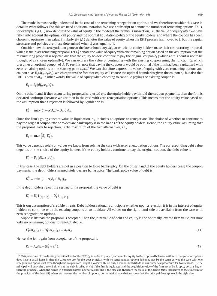
We first explain the qualitative effects of having one renegotiation option insisting that the renegotiation is based on crediblethreats. The effect is best understood if we let all the bargaining power reside with equity holders, i.e., we set γ = 1. All otherinput parameters are given in Table 1. We focus at the value functions near the optimal renegotiation boundary. Fig. 1 depicts theoptimally levered firm value with zero remaining renegotiation options (A0ξ). We also show the liquidation value ((1 − α)A0ξ).For all values of EBIT above the optimal renegotiation boundary (ξ = d1ξ0 = 0.272), equity holders prefer to continue with theexisting coupon rather than to liquidate the firm (i.e., E1c N E1

b). Since debt holders know it is in the best interest of equity holdersto continue servicing the debt with zero remaining options, they will reject renegotiation proposals, based on a liquidation threat,made when ξ N d1ξ0). Hence, equity holders optimally postpone their renegotiation offer to the point at which liquidationbecomes a credible threat (i.e., ξ = d1ξ0). In this way, they maximize the value of their remaining renegotiation option. As aconsequence, the debt value (D1 and also D1

c) is larger than the liquidation value for values of ξ above, but close to, therestructuring boundary d1ξ0. This is what separates our model based on credible threats from a model in which the threat ofliquidation is not necessarily credible. In a strategic debt service model based on non-credible liquidation threats, the debtrenegotiation offer may be proposed at a higher level of ξ than d1ξ0. This implies that in these models, the debt value is alwayslower than the total liquidation value of the firm.

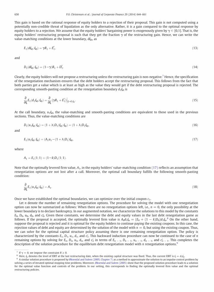
How large, then, are the quantitative effects of debt renegotiation backed by credible threats? Fig. 2 depicts the debt andequity values as well as the optimal coupon and the renegotiation and call boundaries as a function of the number ofrenegotiation options. The optimal coupon, the optimal leverage, and the optimally levered firm value all increase significantlygoing from a setting with liquidation at the lower boundary (n = 0) to a setting with one renegotiation option (n = 1). Furtherincreasing the number of renegotiation options has only a minor effect on all relevant quantities. The ex-ante value of theincreased leverage can be measured by the dollar tax advantage to debt (TAD) defined as the difference between the optimallylevered firm value and the unlevered firm value. TAD increases from 2.04 with n = 0 to 2.83 with n = 1 and 3.06 with n = 8.Hence, the possibility of debt renegotiation increases TAD by 50% even when debt renegotiation proposals must be backed bycredible threats.

To analyze the effect of insisting on credible threats, we have compared the numerical results of our model to a version of ourmodel based on strategic debt service. That is, a model similar to ours except for the fact that equity holders can make

E1c

E1

D1

1 A0

A0

E1b

0.4 0.6 0.8 1.0

5

10

15

20

Value

ξ

ξ

ξ

Fig. 1. The value functions of the claims of the firm. The value functions are depicted as a function of the current EBIT value, ξ. The figure concentrates on the valuefunctions for low values of EBIT between the lower renegotiation (or bankruptcy) boundary and the initial value, ξ = 1. All parameters are as in the base case inTable 1, except that all the bargaining power reside with the equity holders, i.e., γ = 1. E1 is the equity value function with one renegotiation option left, D1 is thedebt value function with one renegotiation option left (since γ = 1, this will also be the value of the debt if the renegotiation proposal is rejected and the equityholders decide to continue with the existing coupon, denoted D1

c in the text), E1c and E1b are the values of equity if their renegotiation proposal is rejected. E1c is the

value if equity holders decide to continue with the existing coupon and E1b is the value if they declare immediate bankruptcy. A0ξ is the optimally levered firm

value if the firm is restructured at ξ, and (1 − α)A0ξ is the optimally levered firm value after liquidation at ξ.

0 2 4 6 8n

0.5

1.0

1.5

2.0

2.5

EBITvalue

cn dn un

0 2 4 6 8n

5

10

15

20

Value

An Dn En TADn

a

b

Fig. 2. Upper and lower restructuring boundaries, optimal coupon rate, and values of claims on the firmat the timewhendebt is issued and the firm's capital structure isoptimized, i.e., when ξ = 1. The values are depicted as a function of the number of renegotiation options, n. All other parameters are as in the base case in Table 1. (a)Upper and lower restructuring boundaries, and the optimal coupon rate. un is the upper restructuring boundary, dn is the lower renegotiation (or for n = 0bankruptcy)boundary, and cn is the optimal coupon. (b) An is optimally levered firm value, Dn is debt value, En is equity value, and TADn is the tax advantage to debt.


restructuring proposals based on a threat of bankruptcy even when it is not in their best interest to do so. The results (notreported here) show that ex-ante values, i.e., total firm value, optimal coupon, and optimal leverage are remarkably similar in thetwo models. However, the trigger for when the equity holders optimally propose a restructuring differs between the two models.With our base case parameters, the trigger for renegotiation is at 0.305, and in the strategic debt service version it is at 0.362. Aswe vary the parameters away from the base case in a comparative static analysis, the trigger for renegotiation varies more in thestrategic debt service case than in our model where we insist on credible threats.

Trade-off models with costs of calling and issuing debt tend to have wide boundaries within which EBIT can fluctuate before thefirm's capital structure is re-optimized. In our base case, the lower renegotiation boundary is at 27% of initial EBIT and debt is calledwhen EBIT has increased by a factor of approximately 2.5. These boundaries narrow only slightly when the number of renegotiationoptions increases. Therefore, the important caveat of Strebulaev (2007) applies, i.e., cross-sectional analysis of leverage ratios, whichdo not recognize that firms are away from their optimal leverage most of the time, may not be consistent with our predictions.

4. Implications for capital structure and APR violations

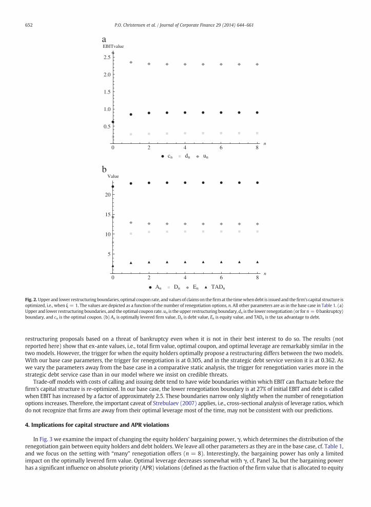
In Fig. 3 we examine the impact of changing the equity holders' bargaining power, γ, which determines the distribution of therenegotiation gain between equity holders and debt holders. We leave all other parameters as they are in the base case, cf. Table 1,and we focus on the setting with “many” renegotiation offers (n = 8). Interestingly, the bargaining power has only a limitedimpact on the optimally levered firm value. Optimal leverage decreases somewhat with γ, cf. Panel 3a, but the bargaining powerhas a significant influence on absolute priority (APR) violations (defined as the fraction of the firm value that is allocated to equity

0.0 0.2 0.4 0.6 0.8 1.0

5

10

15

20

Value

A D E TAD

γ

γ γ0.0 0.2 0.4 0.6 0.8 1.0

0.05

0.10

0.15

0.20

0.25

APR Violations

0.0 0.2 0.4 0.6 0.8 1.0

0.1

0.2

0.3

0.4

0.5

0.6

Recovery rate

a

b c

Fig. 3. Values of claims on the firm, APR violations, and debt recovery rates as a function of the bargaining power distribution between equity holders and debtholders, γ. All other parameters are as in the base case in Table 1. γ = 1 means that the equity holders have all the bargaining power whereas γ = 0 means thatdebt holders have all the bargaining power. (a) A is total firm value, D is debt value, E is equity value, and TAD is the tax advantage to debt at the time when debt isissued and the firm's capital structure is optimized, i.e., when ξ = 1. (b) The fraction of the firm value that is allocated to equity at the time of renegotiation, i.e., ameasure of the APR violation. (c) The recovery rate of the debt (relative to principal) at the time of renegotiation.


at the time of renegotiation), cf. Panel 3b. Lowering the equity holders' bargaining power from one down to zero reduces the sizeof the absolute priority violation virtually linearly down to zero as well. When the firm's capital structure is optimized, theobjective is total firm value maximization. Therefore, it is not a first-order effect how equity holders and debt holders eventuallyshare the firm value at each renegotiation. Consequently, the optimally levered firm value does not vary with the equity holders'bargaining power, γ. On the other hand, equity holders postpone their renegotiation proposal until the threat of liquidationbecomes credible and, hence, at each round of renegotiations equity holders get a fraction, γ of the saved bankruptcy costs.

Note from Panel 3c that the recovery rate of debt in renegotiation (defined as the fraction of debt principal received by debtholders at the time of renegotiation) is relatively unaffected by the equity holders' bargaining power. This is because thebargaining power only determines the allocation of the renegotiation gains, i.e., debt holders get the liquidation value of the firmplus their fraction of the renegotiation gain.

Empirical research reveals that APR violations are common, but recent evidence also points to the fact that violations havebecome less frequent and of smaller magnitude. In the 1980s, APR violations occur as often as in 75% of the U.S. Chapter 11 casesand equity received on average 7.6% of the reorganized firm's value, see Franks and Torous (1989, 1994), Eberhart et al. (1990),Weiss (1990), and Betker (1995). Within the last decade, however, Bharath et al. (2010) report that the empirical evidence onAPR violations has changed. In the period 1991–2005, the average frequency of violations decreased to 22%. Also, the magnitudeof absolute priority violations has declined from 10 % of firm value to less than 2% of firm value. Bharath et al. (2010) suggest thatthese changes are due to Chapter 11 becoming more creditor friendly in recent years, e.g., due to increasing reliance ondebtor-in-possession (DIP) financing. Similarly, Senbet and Wang (2010) point to the fact that there have been severalinnovations related to the bankruptcy reorganization process in recent years starting in the 1990s. The essence is that creditorshave gained stronger bargaining power in the recent years at the expense of equity holders. While our model can only make the

0.0 0.1 0.2 0.3 0.4 0.5

5

10

15

20

Value

A D E TAD

0.0 0.1 0.2 0.3 0.4 0.5

0.05

0.10

0.15

0.20

0.25

APR Violations

0.0 0.1 0.2 0.3 0.4 0.5

0.1

0.2

0.3

0.4

0.5

0.6

Recovery rate

a

b c

α

α α

Fig. 4. Values of claims on the firm, APR violations, and debt recovery rates as a function of the bankruptcy costs, α. All other parameters are as in the base case inTable 1. (a) A is total firm value, D is debt value, E is equity value, and TAD is the tax advantage to debt at the time when debt is issued and the firm's capitalstructure is optimized, i.e., when ξ = 1. (b) The fraction of the firm value that is allocated to equity at the time of renegotiation, i.e., a measure of the APRviolation. (c) The recovery rate of the debt (relative to principal) at the time of renegotiation.


APR violations disappear by assigning zero bargaining power to equity holders—and therefore has less to say about the frequencyof violations—it clearly implies that lowering the bargaining power lowers the size of the APR violations. Note also, that the size ofthe violation is still small relative to firm value, and therefore, the recovery value of debt is fairly insensitive to the bargainingpower of equity holders. The strength of the position of creditors in a bankruptcy or renegotiation is often proxied by creditordispersion, and we would therefore expect to see no significant effect of creditor dispersion on recovery values of debt. This isconsistent with the evidence found in Acharya et al. (2007). In summary, the distribution of bargaining power, γ, has only a minorimpact on the capital structure choice and on debt recovery, but it significantly affects the size of the APR violation.

Bankruptcy costs, α, turn out to play a role similar to that of the bargaining power, γ. As we learn from Fig. 4, bankruptcy costshave a limited impact on the choice of capital structure and debt recovery, but they do affect the size of the APR violation.Lowering the bankruptcy costs down to zero reduce the size of the absolute priority violation virtually linearly down to zero aswell.

On the equilibrium path the firm's capital structure will be renegotiated n times before bankruptcy may eventually occur.Hence, from an ex-ante perspective the present value of the bankruptcy costs are very small. On the other hand, off theequilibrium path, equity holders effectively threaten to declare immediate bankruptcy (in the sense that they wait to proposetheir renegotiation proposal until the threat of liquidation becomes credible) and, hence, at each round of renegotiations, equityholders get half (in general a share equal to γ) of the saved bankruptcy costs.

In Fig. 5 we examine the impact of the volatility of EBIT. Volatility does not affect the size of the APR violations, and it has only alimited effect on debt recovery, again consistent with the empirical evidence found in Acharya et al. (2007). Unsurprisingly, ahigher volatility increases the equity value, and it decreases the leverage and thereby the tax advantage to debt. Unreportedresults show that yield spreads increase, while the renegotiation boundary decreases in the volatility. These results are consistentwith other dynamic capital structure models. In models with no debt renegotiation, the equity holders receive no value at the

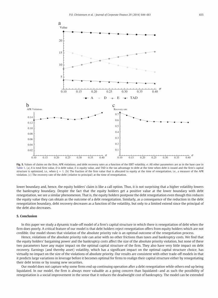
0.10 0.15 0.20 0.25 0.30 0.35 0.40

5

10

15

20

Value

A D E TAD

0.10 0.15 0.20 0.25 0.30 0.35 0.40

0.02

0.04

0.06

0.08

0.10

0.12

0.14

APR Violations

0.10 0.15 0.20 0.25 0.30 0.35 0.40

0.1

0.2

0.3

0.4

0.5

0.6

0.7

Recovery rate

a

b c

σ

σ σ

Fig. 5. Values of claims on the firm, APR violations, and debt recovery rates as a function of the EBIT volatility, σ. All other parameters are as in the base case inTable 1. (a) A is total firm value, D is debt value, E is equity value, and TAD is the tax advantage to debt at the time when debt is issued and the firm's capitalstructure is optimized, i.e., when ξ = 1. (b) The fraction of the firm value that is allocated to equity at the time of renegotiation, i.e., a measure of the APRviolation. (c) The recovery rate of the debt (relative to principal) at the time of renegotiation.


lower boundary and, hence, the equity holders' claim is like a call option. Thus, it is not surprising that a higher volatility lowersthe bankruptcy boundary. Despite the fact that the equity holders get a positive value at the lower boundary with debtrenegotiation, we see a similar phenomenon. That is, the equity holders postpone the debt renegotiation even though this reducesthe equity value they can obtain as the outcome of a debt renegotiation. Similarly, as a consequence of the reduction in the debtrenegotiation boundary, debt recovery decreases as a function of the volatility, but only to a limited extend since the principal ofthe debt also decreases.

5. Conclusion

In this paper we study a dynamic trade-off model of a firm's capital structure in which there is renegotiation of debt when thefirm does poorly. A critical feature of our model is that debt holders reject renegotiation offers from equity holders which are notcredible. Our model shows that violation of the absolute priority rule is an optimal outcome of the renegotiation process.

Hence, violations of the absolute priority rule can arise with no other frictions than taxes and bankruptcy costs. We find thatthe equity holders' bargaining power and the bankruptcy costs affect the size of the absolute priority violation, but none of thesetwo parameters have any major impact on the optimal capital structure of the firm. They also have very little impact on debtrecovery. Earnings (and thereby asset) volatility, which has a significant impact on the optimal capital structure choice, hasvirtually no impact on the size of the violations of absolute priority. Our results are consistent with other trade-off models in thatit predicts large variations in leverage before it becomes optimal for firms to realign their capital structure either by renegotiatingtheir debt terms or by issuing new securities.

Our model does not capture why some firms end up continuing operation after a debt renegotiation while others end up beingliquidated. In our model, the firm is always more valuable as a going concern than liquidated—and as such the possibility ofrenegotiation is a social improvement in the sense that it reduces the deadweight cost of bankruptcy. The model can be extended


in at least two ways to include this feature. Either we can introduce an exogenously given probability that the debt and equityholders cannot reach an agreement of how to restructure the firm, or we can introduce a second state variable measuring thevalue of the firm's assets. In the latter case, the firmmay be liquidated simply because the firm's assets are more valuable than thepresent value of the EBIT process optimally levered. For example, the assets may be used for some other purpose than generatingthe current EBIT. One attempt in this direction is Flor (2008).

Acknowledgments

The paper benefitted greatly from comments from the editors Itay Goldstein and Dirk Hackbarth as well as an anonymousreferee. We are grateful for discussions at the Norwegian School of Economics and Business Administration, Copenhagen BusinessSchool, the EFA Doctoral Tutorial, the University of Vienna, the Norwegian School of Management, The Anderson School at UCLA,meetings of the Bachelier Finance Society, EFA, CEPR, and the Econometric Society. We are grateful to Peter Bossaerts, MichaelBrennan, Bhagwan Chowdhry, Mark Garmaise, Mark Grinblatt, Matthias Kahl, Richard Roll, Eduardo Schwartz, and other seminarparticipants for valuable comments and suggestions. The authors gratefully acknowledge financial support of the Danish SocialScience Research Council. Lando and Miltersen acknowledge support from the Center for Financial Frictions (FRIC), grant no.DNRF102.

Appendix A. Fixed point solution to the pricing of debt and equity

To set up some notation, we quickly reiterate parts of the standard theory. First, consider a very simple claim paying one unitof account when ξ hits the lower boundary, ξ, but only if the lower boundary has been hit before the upper boundary, ξ. The price,denoted P , of this claim as a function of the current level of EBIT, ξ, can be derived as

where

and

with t

P ξð Þ ¼ −ξx2ξx1 þ ξ

x1ξx2

Σ; ξ∈ ξ; ξ

h i;

x1 ¼12σ

2−μ� �

þffiffiffiffiffiffiffiffiffiffiffiffiffiffiffiffiffiffiffiffiffiffiffiffiffiffiffiffiffiffiffiffiffiffiffiffiffiffiμ−1

2σ2

� �2 þ 2rσ2q

σ2 ;

x2 ¼12σ

2−μ� �

−ffiffiffiffiffiffiffiffiffiffiffiffiffiffiffiffiffiffiffiffiffiffiffiffiffiffiffiffiffiffiffiffiffiffiffiffiffiffiμ−1

2σ2

� �2 þ 2rσ2q

σ2 ;

Σ ¼ ξx1ξ x2−ξx1ξ

x2 :

This follows from the fact that P solves the linear ordinary differential equation (ODE)

12σ2ξ2P VV ξð Þ þ μ ξP V ξð Þ−rP ξð Þ ¼ 0; ðA:1Þ

he boundary conditions

P ξ� �

¼ 1 and P ξ� �

¼ 0:

Similarly, interchanging the boundary conditions, we find the price of a claim paying one unit of account when ξ hits the upperboundary, ξ, but only if the upper boundary has been hit before the lower boundary, ξ. The price, denoted P, of this claim as afunction of the current level of EBIT, ξ, can be derived as

P ξð Þ ¼ ξx2ξx1−ξx1ξx2

Σ; ξ∈ ξ; ξ

h i:

We also need a claim that pays a dividend stream at the rate δξs + b at any date s ∈ [t,∞). The date t value of this claim caneasily be derived (either using risk neutral expectations or Gordon's formula) as

Δξt þ B;

where

for an

10 Alte

with th

Re

where

and

11 ThaThe reabounda


Δ ¼ δr−μ

and B ¼ br:

With these three claims priced we are able to price all claims of interest in our model. Consider the claim which pays off adividend stream at the rate δξt + b at any date, t, until one of the boundaries has been hit. When it hits one of the boundaries, itpays out a final lump-sum payment. If the lower boundary, ξ, has been hit first, it pays out F, and if the upper boundary, ξ, has beenhit first, it pays out F. The price, denoted F �; δ; b; ξ; F ; ξ; F

� �, of this claim as a function of the current level of EBIT, ξ, can easily be

derived as

F ξ; δ; b; ξ; F ; ξ; F� �

¼ Δξþ Bþ F−Δξ−B� �

P ξð Þ þ F−Δξ−B� �

P ξð Þ; ξ∈ ξ; ξh i

: ðA:2Þ

Eq. (A.2) has the following easy interpretation: The date t value of getting the dividend stream at the rate δξs + b at any dates ∈ [t, ∞) is Δξt + B. Eventually ξ will hit either ξ or ξ. If, e.g., ξ has been hit first, the claim pays out F and the rest of the dividendstream (with a value of Δξ þ B) is forgone. The net present value of this seen from date t is F−Δξ−B

� �P ξtð Þ. The same argument

applies for the upper boundary, ξ.Plugging in the definitions of P and P reveals10

F ξ; δ; b; ξ; F ; ξ; F� �

¼ 1Σ

F−Δξ−B� �

ξx2− F−Δξ−B� �

ξx2� �

ξx1 þ 1Σ

F−Δξ−B� �


ξx1� �

ξx2

þ Δξþ B; ξ∈ ξ; ξh i

:ðA:5Þ

A very useful property of the price function, F, is the following positive homogeneity of degree one property

F hξ; δ;hb; hξ;hF ; hξ;hF� �

¼ hF ξ; δ; b; ξ; F ; ξ; F� �

; A:6

y ξ∈ ξ; ξh i

and h ∈ ℝ+. This is very easily checked by directly applying Eq. (A.5).11

F ξ; δ; b; ξ; F ; ξ; F� �

¼ k1ξx1 þ k2ξ

x2 þ δξr−μ

þ br; ξ∈ ξ; ξ

h i; ðA:4Þ

The economic intuition behind this homogeneity property is quite trivial: if the unit of account was changed, e.g., from $ to €,on all inputs, then also the value will change accordingly from being measured in $ to being measured in €. This result heavily

rnatively, Eq. (A.5) can be derived by observing that F is the solution to the inhomogeneous ODE (suppressing δ, b, ξ, F , ξ, and F in the notation for F)

12σ2ξ2 F″ ξð Þ þ μξF ′ ξð Þ−rF ξð Þ þ δξþ b ¼ 0;

e boundary conditions

F ξ� �

¼ F and F ξ� �

¼ F:

call that the general solution to the ODE (A.3) is

F ξ; δ; b; ξ; F ; ξ; F� �

¼ k1ξx1 þ k2ξ

x2 þ δξr−u

þ br; ξ∈ ξ; ξ

h i;

k1 and k2 are determined by the boundary conditions. Simple manipulations reveal that

k1 ¼ 1Σ

F−Δξ−B� �


ξx2

� �

k2 ¼ 1Σ

F−Δξ−B� �

ξx1− F−Δξ−B

� �ξx1

� �:

t it is true for any ξ∈ ξ; ξ� �

follows directly. That it is also true for ξ∈ ξ; ξn o

must be checked separately. It comes from the fact that F ξ� �

¼ F and F ξ� �

¼ F.son why, e.g., F ξ

� �¼ F is because if ξ ¼ ξ then the upper boundary is hit immediately and therefore (i) there is no waiting time until one of the two

ries will be hit and (ii) there is zero probability that the lower boundary will be hit before the upper boundary.


relies on the scaling invariant feature of the geometric Brownian motion and that everything except for monetary units isspecified in rates.

With this machinery in place we return to the problem of finding the optimal dynamic capital structure of the firm and thevalues of debt and equity. Basically, debt and equity are claims of the form F just derived. We just have to find δ, b, ξ, F, ξ, and F forboth debt and equity.

In order to find the after-tax payout rate, δξ + b, on debt and equity we need to know the tax rules and payout rates. Here, webriefly recap the structure from Section 2. Coupon payments paid out to the debt holders are expenses for the firm, i.e. they aresubtracted from the EBIT before the firm pays corporate tax. Hence, the total tax paid on coupons is the personal interest tax paidby the debt holders. For dividends the firmmust first pay tax on its EBT before dividends can be paid out to the equity holders. Ontop of that the equity holders pay dividend tax on dividends paid out. Hence, the after-tax payout rate, δξ + b, on debt is specifiedas

and fo

Table AValues f

DEξ ≥ C

Eξ bC

D + ED + E

δξþ b ¼ 1−τið ÞC

r equity it is specified as

δξþ b ¼ 1−τeð Þ ξ−Cð Þ; if ξ≥C;1−�ϵτeð Þ ξ−Cð Þ; if ξbC:

�

Here τe denotes the effective tax rate on dividends. That is,

τe ¼ τc þ 1−τcð Þτd;

τc denotes the corporate tax rate, and τd denotes the personal dividend tax rate. � denotes the effective tax refund when
whereEBT is negative. The values assigned to δ and b for debt and equity are summarized in Table A.1. By adding the payout rates of debtand equity we see that there is a tax advantage to debt if and only if the effective tax rate on dividends is higher than the personaltax on interest payments, i.e. τe N τi, when EBT is positive, i.e. ξ ≥ C. However, for ξ b C it is possible that there can be a taxdisadvantage to debt. This happens when �τe b τi. For the rest of the paper we assume that τe N τi such that there is a taxadvantage to debt for positive EBT. This implies that the optimal capital structure of the firm will include some debt.
For a given (optimal) coupon rate, C⁎, on the debt, and a given restructuring policy, ξ; ξ� �

(determined endogenously in themodel when the debt was issued, e.g. at date zero when the EBIT process was ξ0), we must specify the value of debt and equitywhen one of the restructuring boundaries has been hit. However, contrary to a static capital structure model these values are notknown since when the restructuring boundaries have been hit, the (possible new) owner will again issue debt and equity andcontinue operation. To establish some notation we denote these values (the notation is obvious) as D, D, E, and E. Furthermore,denote the earliest date after the debt issue when a restructuring boundary has been hit as τ. Since the situation at date τ, whenthe (possible new) owner of the whole firm reissues new debt, is exactly identical to the situation at date zero when the originalentrepreneur issued the original debt—except that the EBIT process is now ξτ instead of ξ0—we conjecture that the coupon rate ofthe newly issued debt will be ξτ

ξ0C∗ at date τ, the new restructuring policy will be ξτ

ξ0ξ; ξτξ0ξ

� �, and the new boundary values will be ξτ

ξ0D,

ξτξ0D, ξτξ0 E , and

ξτξ0E. In fact, we will later prove that this conjecture is correct. We state our conjecture formally below.

Conjecture 1.

1. The optimal coupon rate C⁎ determined just prior to issuing the debt at a given date s when the EBIT process is ξs can bewritten as

C� ¼ c�ξs;

a given constant c⁎. � �
for2. The incentive compatible restructuring policy ξ; ξ , which is common knowledge as soon as the coupon rate C⁎ is fixed at a given
date s when the EBIT process is ξs, can be written as

ξ ¼ dξs

.1or δ and b for debt (D) and equity (E) both when EBT is positive and when it is negative.

δ b

0 (1 − τi)C1 − τe −(1 − τe)C1 − �τe −(1 − �τe)C

ξ ≥ C 1 − τe (τe − τi)Cξ bC 1 − �τe (�τe − τi)C

and

and

and

and

12 Forway canas E(c∗ξ13 If c∗


ξ ¼ uξs;

given constants d ∈ (0,1) and u ∈ (1,∞).
for3. The values of debt and equity when one of the boundaries (induced by the commonly known restructuring policy fixed by the
optimally determined coupon rate at a given date s when the EBIT process is ξs) has been hit can be written as

D ¼ dξs;D ¼ dξs;E ¼ eξs;

E ¼ eξs;given constants d, d, e, and e.
for
Given Conjecture 1 we can derive (and denote) the price at any given date t, when the EBIT process is ξt, of debt and equityissued at some date s ≤ t, when the EBIT process was ξs, provided that the EBIT process {ξu}u ∈ [s,t] in the time period [s,t) hasstayed inside the interval (dξs, uξs), as

D ξt ; ξsð Þ ¼ F ξt ;0; 1−τið Þc�ξs;dξs; dξs;uξs;dξs� �

E ξt ; ξsð Þ ¼ F ξt ;1−τe;− 1−τeð Þc�ξs;dξs; eξs;uξs; eξs� �

: ðA:7Þ

To be exact, the equity value, E, has only the form (Eq. (A.7)) if c∗ ≤ d. This is due to the asymmetric tax regime the equityholders' face. They have to pay the tax rate τe when the firm's EBT is positive, but they can only deduct at the tax rate �τe when thefirm's EBT is negative. Hence, if c∗ ∈ (d,u), the equity value is pieced together in the following way to ensure that it is one-timecontinuously differentiable

E ξt ; ξsð Þ ¼ F ξt ;1−�ϵτe;− 1−�ϵτeð Þc�ξs;dξs; eξs; c�ξs; e�ξs� �

; if ξtbc�ξs;

F ξt ;1−τe;− 1−τeð Þc�ξs; c�ξs; e�ξs;uξs; eξs� �

; if ξt≥c�ξs:

�ðA:8Þ

Here, e∗ is the equity value when ξt = c∗ and ξs = 1. This value is determined by requiring the equity value function, E, to becontinuously differentiable in the first variable at the point ξt = c∗ξs.12 Finally, if c∗ ≥ u, the firm always has negative earnings netof coupon payments, so E has the form E ξt ; ξsð Þ ¼ F ξt ;1−�ϵτe;− 1−�ϵτeð Þc∗ξs;dξs; eξs;uξs; eξsð Þ:

Appendix B. Verification of Conjecture 1

In this appendix we verify that there exists solutions to debt and equity that fulfills Conjecture 1. Eqs. (5), (6), (7), and (8)immediately verify part 3 of Conjecture 1 and that

d ¼ min 1−αð ÞAd;Df g;d ¼ 1þ λð ÞD;e ¼ max 1−αð ÞAd−D;0f g;

e ¼ Au− 1þ λð ÞD:

For given c∗, d, and u, the two constants D and E can be found by solving for the initial debt and equity values for ξt = ξs = 1.That is, using the expression of F from Eq. (A.2) we have the following two equations in two unknowns13

D ¼ ΔDð 1−dP 1ð Þ−uP 1ð Þ� �þ BD 1−P 1ð Þ−P 1ð Þ� �þmin 1−αð ÞAd;Df gP 1ð Þ þ 1þ λð ÞDP 1ð Þ

mally, we have to add the condition that the equity value at the point where the two parts are pieced together in a one-time continuously differentiablebe written as e∗ξs to our Conjecture 1. That is, we have to add to part 3 of Conjecture 1 that the value of equity, at the point where ξt = c∗ξs, can be written

s; ξs) = e∗ξs for a given constant e∗.∈ (d,u), there are three unknowns: D, E, and e∗. The third equation comes from differentiability of the equity function, E, at ξt = c∗ξs, cf. Eq. (A.8).

and

That isto issugives e

Pluggi

¼ argc∈

Note tConjeclevel ξsolutioBecaufixed-

14 In famissing


E ¼ ΔE 1−dP 1ð Þ−uP 1ð Þ� �þ BE 1−P 1ð Þ−P 1ð Þ� �þmax 1−αð ÞAd−D;0f gP 1ð Þ þ Au− 1þ λð ÞDð ÞP 1ð Þ:

Here,

ΔD ¼ 0; ΔE ¼ 1−τeð Þr−μ

; BD ¼ c�

r; and BE ¼ − 1−τeð Þc�

r:

For a given c∗, we can find d and u by the two smooth pasting conditions, Eqs. (9) and (10). Unfortunately, these two equationsin two unknowns can only be solved numerically. However, by Euler's theorem E1(ξt;ξs) is positive homogeneous of degree zerobecause E(ξt;ξs) itself is positive homogeneous of degree one, cf. Eq. (3). That is,

E1 hξt ;hξsð Þ ¼ E1 ξt ; ξsð Þ;

y ξt ∈ [dξs, uξs] and h∈Rþ . Hence, Eqs. (9) and (10) are identical independent of the actual level of ξ0. Therefore, the
for ansolutions d and u are also independent of the actual level of ξ0. That is, we have verified part 2 of Conjecture 1.14 Finally, theoptimal coupon rate of the debt, which is determined just prior to the debt issue at date zero, is given by
C� ¼ argmaxC∈Rþ

A ξ0ð Þ:

so because it is the original entrepreneur who determines the coupon rate of the perpetual debt that he or she would likee. Naturally, the entrepreneur sets the coupon rate in order to maximize his or her own value. Moreover, rewriting C as cξ0xactly the same optimization problem since ξ0 is positive

C� ¼ argmaxC∈Rþ

A ξ0ð Þ ¼ ξ0 argmaxC∈Rþ

A ξ0ð Þξ0

!:

ng in the definition of A(ξ0) from Eq. (4) gives

c� ¼ argmaxc∈Rþ

E ξ0; ξ0ð Þ þ 1−kð ÞD ξ0; ξ0ð Þξ0

maxRþ

F ξ0;1−τe;− 1−τeð Þcξ0;d cð Þξ0; e cð Þξ0;u cð Þξ0; e cð Þξ0ð Þξ0

þ 1−kð ÞF ξ0;0; 1−τið Þcξ0;d cð Þξ0; d cð Þξ0;u cð Þξ0; d cð Þξ0� �

ξ0

0@

1A

¼ argmaxc∈Rþ

F 1;1−τe;− 1−τeð Þc;d cð Þ; e cð Þ;u cð Þ; e cð Þð Þ þ 1−kð ÞF 1;0; 1−τið Þc;d cð Þ; d cð Þ;u cð Þ; d cð Þ� ��

:

hat we have emphasized the dependence of d, u, d , d, e, and e on the given coupon rate parameter, c, cf. part 2 and 3 ofture 1. Finally, notice that the optimal coupon rate parameter, c∗, in the above optimization is independent of the initial0 so we have verified the missing part (part 1) in Conjecture 1. That is, we have now verified that there exists a fixed-pointn to our debt and equity valuation problem giving us solutions to the value of debt and equity fulfilling Conjecture 1.se of our conjecture-verification method of finding the fixed-point solution, we cannot rule out that there might be otherpoint solutions which do not fulfill Conjecture 1.

References

Acharya, V., Bharath, S., Srinivasan, A., 2007. Does industry-wide distress affect defaulted firms? Evidence from creditor recoveries. J. Financ. Econ. 85, 787–821.Altman, E.I., Hotchkiss, E., 2010. Corporate Financial Distress and Bankruptcy: Predict and Avoid Bankruptcy, Analyze and Invest in Distressed Debt, 3rd ed. John

Wiley & Sons Inc.Anderson, R.W., Sundaresan, S., 1996. Design and valuation of debt contracts. Rev. Financ. Stud. 9, 37–68.Annabi, A., Breton, M., François, P., 2010. Resolution of Financial Distress under Chapter 11. Working Paper 10-48. CIRPÉE.Betker, B.L., 1995. Management's incentives, equity's bargaining power, and deviations from absolute priority rule in chapter 11 bankruptcies. J. Bus. 68, 161–183.Bharath, S., Panchapegesan, V., Werner, I., 2010. The Changing Nature of Chapter 11. Working Paper. Ohio State University, Charles A. Dice Center for Research in

Financial Economics.Black, F., Cox, J., 1976. Valuing corporate securities: some effects of bond indenture provisions. J. Finance XXXI, 351–367.

ct, this positive homogeneity property of degree zero of E1(ξt;ξs) can also be used to verify that e∗ is independent of the actual level of ξ0. This verifies theconjecture in the case where c∗ ∈ (d,u), cf. footnote 32.

http://refhub.elsevier.com/S0929-1199(13)00083-7/rf0005










Brekke, K.A., Øksendal, B., 1991. The high contact principle as a sufficiency condition for optimal stopping. Stochastic Models and Option Value. Elsevier SciencePublishers, B. V., North-Holland, Amsterdam, The Netherlands, pp. 187–208.

Brekke, K.A., Øksendal, B., 1994. Optimal switching in an economic activity under uncertainty. SIAM J. Control. Optim. 32, 1021–1036.Bris, A., Welch, I., Zhu, N., 2006. The costs of bankruptcy: chapter 7 liquidation versus chapter 11 reorganization. J. Finance 61, 1253–1303.Broadie, M., Chernov, M., Sundaresan, S., 2007. Optimal debt and equity values in the presence of chapter 7 and chapter 11. J. Finance 62, 1341–1377.Dixit, A., 1991. A simplified treatment of the theory of optimal regulation of brownian motion. J. Econ. Dyn. Control. 15, 657–673.Dixit, A.K., 1993. The Art of Smooth Pasting. Harwood Academic Publishers.Dockner, E., Mæland, J., Miltersen, K.R., 2013. Interaction between dynamic financing and investments: the impact of industry structure. Working Paper.

Copenhagen Business School.Eberhart, A., Moore, W., Roenfeldt, R., 1990. Security pricing and deviations from the absolute priority rule in bankruptcy proceedings. J. Finance XLV, 1457–1469.Fischer, E.O., Heinkel, R., Zechner, J., 1989a. Dynamic capital structure choice: theory and tests. J. Finance XLIV, 19–40.Fischer, E.O., Heinkel, R., Zechner, J., 1989b. Dynamic recapitalization policies and the role of call premia and issue discounts. J. Financ. Quant. Anal. 24, 427–446.Flor, C.R., 2008. Capital structure and assets: effects of an implicit collateral. Eur. Financ. Manage. 14, 347–373.Flor, C.R., Lester, J., 2002. Debt Maturity, Callability, and Dynamic Capital Structure. Working Paper. Dept. of Business and Economics, University of Southern

Denmark, Campusvej 55, 5230 Odense M, Denmark.François, P., Morellec, E., 2004. Capital structure and asset prices: some effects of bankruptcy procedures. J. Bus. 77, 387–411.Franks, J., Torous, W., 1989. An empirical investigation of firms in reorganization. J. Finance XLIV, 747–779.Franks, J., Torous, W., 1994. A comparison of financial recontracting in distressed exchanges and chapter 11 reorganizations. J. Financ. Econ. 35, 347–370.Galai, D., Raviv, A., Wiener, Z., 2007. Liquidation triggers and the valuation of debt and equity. J. Bank. Finance 31, 3604–3620.Gilson, S., John, K., Lang, L., 1990. Troubled debt restructurings: an empirical study of private renegotiation of firms in default. J. Financ. Econ. 27, 315–353.Goldstein, R., Ju, N., Leland, H.E., 2001. An ebit-based model of dynamic capital structure. J. Bus. 74, 483–512.Hackbarth, D., Hennessy, C.A., Leland, H.E., 2007. Can the tradeoff theory explain debt structure? Rev. Financ. Stud. 20, 1389–1428.Hege, U., Mella-Barral, P., 2005. Repeated dilution of diffusely held debt. J. Bus. 78, 737–786.Kane, A., Marcus, A.J., McDonald, R.L., 1985. Debt policy and the rate of return premium to leverage. J. Financ. Quant. Anal. 20, 479–499.Leland, H.E., 1994. Corporate debt value, bond covenants, and optimal capital structure. J. Finance XLIX, 1213–1252.Lemmon, M.L., Roberts, M.R., Zender, J.F., 2008. Back to the beginning: persistence and the cross-section of corporate capital structure. J. Finance 63, 1575–1608.Mella-Barral, P., 1999. The dynamics of default and debt reorganization. Rev. Financ. Stud. 12, 535–578.Mella-Barral, P., Perraudin, W.R.M., 1997. Strategic debt service. J. Finance LII, 531–556.Merton, R.C., 1973. Theory of rational option pricing. Bell J. Econ. Manag. Sci. 4, 141–183 (reprinted in (Merton, 1990, Chapter 8)).Merton, R.C., 1974. On the pricing of corporate debt: the risk structure of interest rates. J. Finance XXIX, 449–470.Miltersen, K.R., Torous, W.N., 2013. Optimal Maturity Structure of Risky Corporate Debt. Working Paper. Copenhagen Business School.Morse, D., Shaw, W., 1988. Investing in bankrupt firms. J. Finance XLIII, 1193–1206.Øksendal, B., Sulem, A., 2005. Applied Stochastic Control of Jump Diffusions. Springer-Verlag, Berlin Heidelberg, Germany.Rubinstein, A., 1982. Perfect equilibrium in a bargaining model. Econometrica 50, 97–109.Rubinstein, A., 1987. A sequential strategic theory of bargaining. Advances in Economic Theory: Fifth World Congress. Cambridge University Press, Cambridge,

Great Britain, pp. 197–224.Senbet, L.W., Wang, T.Y., 2010. Corporate financial distress and bankruptcy: a survey. Found. Trends Finance 5, 243–335.Strebulaev, I.A., 2007. Do tests of capital structure theory mean what they say? J. Finance 62, 1747–1787.Weiss, L.A., 1990. Bankruptcy resolution: direct costs and violations of priority of claims. J. Financ. Econ. 27, 285–314.








































Dynamic capital structure with callable debt and debt renegotiations

Documents

Transcript of Dynamic capital structure with callable debt and debt renegotiations