The debt crisis: a re-appraisal

The Developing Economies

, XLVI-3 (September 2008): 290–314

© 2008 The Authors doi: 10.1111/j.1746-1049.2008.00067.xJournal compilation © 2008 Institute of Developing Economies

Blackwell Publishing LtdOxford, UKDEVEDeveloping Economies0012-15331746-10492008 The AuthorsJournal compilation © 2008 Institute of Developing EconomiesXXX Original Articles

delays in stabilization or in reforms?THE DEVELOPING ECONOMIES

DELAYS IN STABILIZATION OR IN REFORMS? THE DEBT CRISIS

Carlos

ALBERTO CINQUETTI

1

and

Ricardo

GONÇALVES SILVA

2

1

Department of Economics, São Paulo State University, São Paulo, Brazil; and

2

Department of Mathematical Modeling, SERASA, São Paulo, Brazil

First version received November 2006; final version accepted March 2008

Empirical analyses attributing the 1980s’ debt crisis to inconsistent stabilization policiesrest on an inappropriate long-run approach. Revising this long-run approach yieldsopposite results: terms of trade shocks and foreign indebtedness explain this crisis,regardless of domestic stabilization policies. This prompts us to consider a new hypothesis,of delays in trade-policy reforms, with a model in which terms-of-trade variation (undershocks) is endogenous to export structure and efficiency of resource allocation. Evidencefrom the structural equations model shows that allocation distortions negatively affectchanges in terms of trade, which then explain this crisis. A political economy extensiondemonstrates that income inequality and regional trade policy determine the distortions,which in turn leads to this crisis.

Keywords

: Debt crisis; Shocks; Stabilization policies; Trade policies; Inequality;Structural equations

JEL classification

: F13, F34, 010

I. INTRODUCTION

T

he

1980s’ debt crisis, a turning point in the development of developingeconomies, is seen as an outcome of trade policies, as reinforced by the factthat it hit almost all countries that were following import-substitution indus-

trialization and only a few following outward-oriented growth (Little, Cooper, andCorden 1994; Krueger 1995). Nonetheless, Berg and Sachs (1988) demonstratedthat both trade openness and variables related to bad stabilization policies help toexplain the observed foreign debt defaults, while external economic vicissitudes

We thank M. Cristina Terra and the two anonymous referees for valuable comments and suggestions.For comments on earlier versions, we also thank Lance Taylor, Kenneth Reinert, Persio Arida, andparticipants at the Encuentro 2005 de la Sociedad de Economía de Chile, VIII ANPEC/SUL in PortoAlegre, as well as Dani Rodrik for providing his database. Financial support from CNPq, FAPESP andFundunesp are gratefully acknowledged.

delays in stabilization or in reforms?

291

© 2008 The AuthorsJournal compilation © 2008 Institute of Developing Economies

(terms of trade shocks and foreign debt burden) were statistically irrelevant. Later,Rodrik (1999a,b) developed a more properly specified empirical model and foundthat trade protection had no significant explanatory power, the same applying toexternal shocks, although shocks are significant within a composite variable stand-ing for political conflicts and indicating delays in stabilization policies.

The statistical insignificance of external shocks alone in Rodrik (1999b) waschallenged by Cinquetti (2005), although it did not tilt the case towards other policydelays, suggesting even that the 1980s’ crisis was caused by

bad luck

: exogenousevents pushing sound economies into crisis.

In the present paper, we reassess the role of microeconomic distortions for the1980s’ debt crisis, proposing a new framework to examine it. The cornerstone of itis to consider terms-of-trade (

TT

) variations among countries not as an equivalent ofexogenous shocks, but as expressive of countries’ economic strength as well, follow-ing a short-run trade model for

TT

changes. This leads to an amplified macroeconomicmodel of balance-of-payments crisis having, in its origin, a microeconomic causation:distortions in resource allocation and economic structure conditioning the impact ofexternal shocks on

TT

. Accordingly, we estimate this theoretical formulation, relatingshocks to the crisis in the presence of microeconomic distortions, by means of astructural two-equation model.

The paper is structured as follows. In Section II we introduce the events asanalyzed in the published literature and empirically reappraise them: correctingsome variables and rerunning the regression model for bad stabilization policies.Having rejected this hypothesis, we then work out, in Section III, the microeconomics-based model for the crisis, grounded in delays in trade-policy reforms, followed byits political extension concerning “what delayed the removal of protectionistpolicies and ultimately led to the crisis?” Estimates of both the positive and thepolitico-economic structural models are presented in Section IV.

II. REEXAMINING THE ECONOMIC DIFFERENCES

In 1978, after a period of plentiful international credit to developing countries,international interest rates started to rise in response to the deteriorating macro-economic environment in developed countries. In 1979, a second oil-price shock tookplace and, in 1980, to make matters even worse, the US government implementedan austere macroeconomic policy, raising real interest rates to 20% from negativevalues, and pushing the world economy into a severe depression. This forced downthe export prices of many developing countries, both oil and non-oil exporting,eventually leading to widespread foreign debt default, triggered by Mexico’s defaultin September 1982. The ensuing stabilization crisis was protracted and generalized,encompassing both recurring balance-of-payments crises and other macroeconomicinstabilities.

292

the developing economies


No expert denied that the losses stemming from the fall in terms of trade and therise in interest rates contributed to the 1980s’ debt crisis. Yet, from the identificationof policy mismanagement in countries that had to reschedule their external debt,Berg and Sachs (1988) worked out an empirical political economic model thatproduced an impressive result: all variables expressing or determining bad policiesshowed statistical significance in predicting the debt crisis, whereas none of theeconomic variables did. This finding and parallel theoretical research helped to shiftresearchers’ attention towards the political environment surrounding policymaking(see Alesina and Perotti 1994).

In the 1990s, economists shifted attention to why economic growth persisted insome countries and not in others. Based on data of the 1960s, 1970s, and 1980s,Easterly

et al

. (1993) found out that terms of trade shocks explain growth variationsand reduce the explanatory power of several variables related to domestic policy andstructural profile, contradicting some findings in Barro (1991). In short, bad luck(i.e., random shocks) also matters.

Rodrik (1999a,b), returning to the debt crisis, focused on changes between 1960–75 to 1975–89, and, most importantly, advanced the first properly specified politicaleconomy model for shocks and delayed stabilization. Basically, it predicts thatsocial conflicts over sharing the losses stemming from external difficulties delay (orweaken) the policy responses and, therefore, lead to crisis. From this development,which concurs with Alesina and Drazen (1991), Rodrik (1999a,b) proposed thefollowing composite variable for empirically measuring conflicts:

(1)

That is, high social cleavages and weak institutions prevent cooperation, magni-fying the conflicts from shocks and delaying the adoption of consistent policies.

In Rodrik’s estimates, terms of trade shocks alone did not explain performance,but could do so within several variations of the above variable for social conflict.Microeconomic distortions (trade protection) were also not statistically significant,enabling him to conclude that “the crisis was the product of monetary and fiscalpolicies” (Rodrik 1999a, p. 77).

It happens that Rodrik’s terms of trade shock, calculated as the standard deviationof the first log-differences of the terms of trade in the 1970s,

1

in no way characterizesthe shocks at stake here. It is displaced in time: the critical changes in

TT

wereconcentrated over the period 1979–81 (see Little, Cooper, and Corden 1994), ratherthan throughout the 1970s. Moreover, taking

TT

shocks as standard deviations,

1

. . . times the

average proportion of total trade to GDP.

This weighting is relevant in the analysis ofeconomic growth, but is not pertinent to balance-of-payment crises.

CONFLICT external shocks social cleavages

institutions of conflict management= ⋅ ⎛⎝

⎞⎠ .


293


regardless of their direction (positive or negative), contradicts all discussions up tothen focused on short-term fall in the

TT

.Keeping to the earlier authors’ perspective, we attempt to reexamine the debt

crisis as a particular balance-of-payment crisis. Accordingly, instead of growthchange after 1975, we take as a dependent variable

RESCH

, a dummy representingwhether or not each country rescheduled its foreign debt with international authorities,borrowed from Berg and Sachs (1988) and shown in Table 1. Besides, given thewidely accepted view that the (generalized) balance-of-payment crises of the 1980sand the late 1990s concerned middle income or large developing economies (Fisher2002), we limit the analysis to them. Contrary to the growth analysis, mentionedabove, neither developed countries nor the small and least developed countries areconsidered, leaving us with the 33 developing countries in Table 1.

2

Except for Yugoslavia and Panama, all the listed countries hit by the crisisunderwent large

TT

falls shortly before the crisis, during the world market depression,

2

Berg and Sachs (1988) actually work with 35 countries, but owing to the lack of data for China andHungary, only 33 countries (see Table 1) were tested for

TT

. We excluded Spain, already classifiedas developed by that time (

World Development Report, 1982

), and reintroduced Hungary from datain

International Financial Statistics

.

TABLE 1

Rescheduling by Regions

East Asia Event Date Latin America Event Date Others Event Date

Hong Kong No 1983 Argentina Yes 1983 Egypt No 1983Indonesia No 1983 Brazil Yes 1983 Hungary No 1983Korea No 1983 Chile Yes 1983 India No 1983Malaysia No 1983 Colombia No 1983 Israel No 1983Philippines Yes 1986 Costa Rica Yes 1983 Ivory Coast Yes 1985Singapore No 1983 Equator Yes 1983 Kenya No 1983Taiwan No 1983 Mexico Yes 1983 Mauritius No 1983Thailand No 1983 Panama† Yes 1983 Morocco Yes 1986

Peru Yes 1983 Portugal No 1983Trinidad-Tobago No 1983 Sri Lanka No 1983Uruguay Yes 1983 Tunisia No 1983Venezuela Yes 1986 Turkey Yes 1983

Yugoslavia† Yes 1983

Average (%) 83 Average (%) 13 Average (%) 29

Source: Berg and Sachs (1988).Note: Yes (No): countries that did (not) reschedule their foreign debt in the indicated year.†Countries that rescheduled their foreign debt, but did not undergo large TT falls during theworld market depression.

294

the developing economies


which stands out as a

debt-deflation crisis

. Accordingly, the impact of the 1979–81shocks on

TT

is measured: the average

TT

over 1982–83 (the crisis and the yearbefore) with respect to the average over 1979–80 or 1980–81 for the oil-exportingcountries (and Portugal) that experienced an upward (in 1980) and downward (in1981–82) fluctuation in their

TT

. This series captures both the oil shock (gains andlosses) and the depression shock according to the position of each of these twogroups of countries.

Foreign indebtedness is another external difficulty to consider, given the view thatexternal shocks led to a generalized payment crisis because of the high external debtburden carried by developing countries in the late 1970s (Cline 1984; Little, Cooper,and Corden 1994). The whole financial dynamic can be referred either to

debt-deflationcrises

(Tobin 1980) or to the instability hypothesis by Minsky (1977): that stableadjustment to adversities depends upon the initial debt structure. Hence, we measurethis burden by “the total debt services to exports of goods and nonfactor services”(

TDSX

) in 1980, at the beginning of the world market recession, whereas Rodrik(1999a,b) take it in 1975, well before the long period of overborrowing. Notice thatthis stock variable,

TDSX

, also conveys accumulated losses from the first oil shock.Therefore, we replicate the above-mentioned political economy test with the

following base line probit model:

(2)

Matrix

EXT

stands for external economic vicissitudes (

TT

shocks and

TDSX

)whose eventual rejection obliges us to test equation (2) with the composite var-iable

CONFLICT

from equation (1). A regional dummy variable for Latin America(

LAM

) is also used, given the exceptional concentration of foreign debt default inthis region,

3

whereas

OPEN

i

(own import-weighted tariff rates on intermediateinputs and capital goods) indirectly expresses the delayed trade-policy reforms.

Finally, the matrix

STAB

, standing for bad stabilization policies, encompassesboth

DIRECT

(direct evidence of lenient macro-policy responses to the 1979–81shocks), and

SOCPOL

(a set of variables standing for circumstances conducive tobad stabilization policies). The following changes from 1980 to 1982 may represent

DIRECT

: in the central government deficits (

DEFCHG

), in the total public and publiclyguaranteed debts (

DODCHG

), and in the consumer prices inflation (

PRCHG

).

4

A setof indicators of social cleavages and institutional strength make up

SOCPOL

, withthe former given by income distribution (

INCDSTR

), measured as the ratio ofincome share of the top 20% of households to the income share of the bottom 20%

3

As in Berg and Sachs (1988), we do not classify Trinidad and Tobago as a Latin American countryin sociocultural terms.

4

All in this form:

g

x

=

(

x

t

–

x

t

–1

)/

x

t

–1

. We found no good measures of exchange rate policies usingcomparative static data, which would be a pure expression of policy.

RESCH OPENi i i .= + ′ + ′ + +β β β β ε0 1 2 3EXT STAB


295


of households around 1980.

5

The murder rate per million inhabitants (

MURDER

)was ignored as it had too many zero values. The indicators of institutional strengthare: (1) the log of public spending on social insurance, averaged over 1975–79(

SOCIAL

), (2) the rule of law (

LAW

), measured on a scale from 0 to 4, expressingthe degree to which citizens are treated as equal under the law and the judiciary, (3)democracy in the 1970s (

DEMOC

), ranging from 0 to 1 (fully democratic system),a composite indicator of civil liberties and political rights, and (4) the index

ICRG

(International Country Risk Guide), based on an underlying numerical evaluationrelating the rule of law, bureaucracy quality, and corruption, whose values rangefrom 0 to 10: higher values meaning superior institutions.

It must be emphasized that, except for the corrections in the two

EXT

variables,equation (2) reproduces the literature. Therefore, its estimates in Table 2 areorganized: models (i) to (iii) test

STAB

as given by

DIRECT

, whereas the remainingones are given by

SOCPOL

. Income distribution is maintained throughout for itschief position in countries’ social matrix, and also because combining two variablesfor institutions of conflict management is meaningless.

What is most remarkable about the new results is that

TT

and

TDSX

are statisticallysignificant in all models, with the predicted signs, negative for the former andpositive for the latter. Hence, debtors’ external economic problems help to predictthe widespread payment crisis in the early 1980s, regardless of countries’ policies.Moreover, their joint statistical significance corroborates the hypothesis of a debtdeflation crisis, as opposed to the late 1990s liquidity crisis that hit solvent debtors(see Fratzscher 1998).

DEFCHG

and

DODCHG are also statistically significant in some specifications,but one can no longer attribute the crisis to bad stabilization policies, in light of theparallel significance of both TT and TDSX. The same applies when proxying STABwith indicators of sociopolitical environment conducive to policy delays (equationsvi to viii). Moreover, only two of these variables for social cleavages and institutionalstrength, ICRG and DEMOC, exhibited statistical significance, with their negative signsconfirming that weak institutions increase the chance of a crisis. In fact, we cannotestablish whether they are associated with indirect pressures on macroeconomicpolicies or with the efficient working of the economy.

Income distribution, INCDSTR, is statistically nonsignificant in all equations,which can be ascribed to its strong correlation with both EXT variables, −0.40 withterms of trade shocks and 0.54 with TDSX, as well as with the dummy for LatinAmerica (0.51). This problem (strong collinearity) does not affect the remainingsocial variables (see Appendix Table 1).

5 We preferred it to the Gini coefficient, which is taken from years far distant from 1980, for somecountries.

296th

e developing econ

omies

© 2008 T

he Authors

Journal compilation ©

2008 Institute of Developing E

conomies

TABLE 2

Probit Estimates of Foreign Debt Crisis†

Independent VariableDependent Variable: Foreign Debt Reschedule

(i) (ii) (iii) (iv) (v) (vi) (vii) (viii)

Constant 7.299* 6.258*** 6.153* 5.435(1.68) (2.63) (1.66) (−1.42)

LAM 1.549** 1.4827* 0.931 1.416** 0.778 0.996 1.77* 2.492***(1.99) (1.926) (1.023) (2.03) (−1.15) (−1.52) (1.77) (2.67)

TT −13.062** −5.8671*** −8.0395* −1.737* −4.239** −4.968** −11.592*** −6.326*(−2.35) (−3.69) (−2.61) (−1.90) (−2.12) (−2.02) (2.59) (−1.68)

TDSX 0.2592** 0.249*** 0.284** 0.105*** 0.106** 0.138* 0.282*** −0.116**(2.322) (2.93) (2.26) (2.95) (2.12) (1.82) (3.07) (2.20)

DEFCHG −0.199 0.4571*** 0.4702*(−0.706) (2.61) (1.86)

PRCHG −0.004(−0.70)

DODCHG 2.9911*** 4.8941***(3.74) (2.60)

OPEN 3.852 −3.516***(1.89) (−0.96)

INCDSTR 0.016 0.026 −0.007 −0.023(−0.55) (−0.71) (−0.21) (−0.59)

SOCIAL 0.621(−1.46)

ICRG −0.737***(−3.60)

LAW −0.1766(−0.63)

DEMOC −4.123**(−2.46)

% Correctly predicted 89.66 96.55 96.30 89.66 90.00 90.32 90.32 80.65Observations 29 30 30 30 30 31 31 31

†Heteroscedasticity corrected models. Constants excluded when not jointly significant or relevant. Values of robust z-statistics in parentheses.***, **, and * represent statistical significance at the 1%, 5%, and 10% level, respectively.

delays in stabilization or in reforms? 297


Except in column (iv), trade openness is not statistically significant in severalvariations of equation (2), corroborating the findings in Rodrik (1999b): that this crisiswas not caused by microeconomic distortions. However, one should not disregardsome data problems in OPEN: the inappropriate weighting of the imported products,noticed by Rodriguez and Rodrik (2001), and the exclusion of consumer goods,which were the most highly taxed in some countries.

III. INTERNAL SOURCES OF EXTERNAL TROUBLES

Political models of monetary and fiscal policies try to explain why similar economicproblems might lead to great differences in macroeconomic performance (Alesina1994). However, as demonstrated, the countries analyzed here were not actuallyfacing similar economic problems: their terms of trade variations and foreignindebtedness were sufficiently different to explain their performance.

It does not follow, however, that this crisis should simply be attributed to bad luck,to circumstances beyond countries’ control. A point disregarded in the examinedempirical literature is that the distinct TT changes across countries, in the wake ofan external shock, may reflect their economic strength. This hypothesis entails anextra endogenous relation, determining TT variations across countries, so that itsestimation would involve a structural model in which a balance-of-payment crisis isultimately rooted in those determinants of TT variation.

A frequently cited reason for TT changes in the turbulent early 1980s was the lowprice-elasticity of commodities and their consequent cyclical oscillations (Labys,Kouassi, and Terraza 2000). In structuralist macroeconomic models (Taylor 1991),this is a micro-foundation for the South’s financial fragility in the wake of theNorth’s monetary restriction, as empirically corroborated by Cristini (1995).

In contrast, orthodox analyses blame microeconomic distortions (i.e., import-substitution industrialization) for the countries’ fates in the 1980s’ crisis. Accordingto Krueger (1995), countries loosely exposed to foreign competition experienced arising ratio of capital to output (K/Y ), eventually leading to growth interruption in the1980s. The argument rests on the standard relationship between distortions andinefficiency, having no bearing on export-price elasticity, or short-run adjustments.We know, however, that the Asian newly industrializing countries’ impressive exportexpansion, without a corresponding deterioration in their TT, was related to successin product differentiation (Riedel and Athukorala 1995). Accordingly, inefficientlate industrialization would be related with failing product differentiation and,therefore, with demand-inelastic exports, which implies TT losses not only in thelong run, as the world income expands, but also in the short run, following a world-market depression.

Summing up, the first argument links price elasticity of demand to manufacturinggoods, whereas the second conditions it to allocative efficiency. From the former, an

298 the developing economies


export structure with a higher share of manufacturing goods shields countriesagainst adverse shocks on their TT, whereas the latter predicts that this depends ona manufacturing industry made up of truly competitive firms, the opposite of an arti-ficially enlarged industry. These two streams of thought are thus called structuralistand orthodox, respectively.

Because each of them rest on price elasticity of demand, it is actually possible tointegrate them into the same theoretical analysis. Consider a two-sector imperfectlycompetitive trade model, with a competitive sector supplying homogenous(agricultural) goods and an imperfectly competitive sector supplying diversifiedmanufacturing goods, the optimal price of which is:

p = θ (τ, n)aw, (3)

where θ is the markup on the marginal cost aw (labor and resource inputs timestheir competitive prices), with θ hinging on price elasticity of demand (τ) and thenumber of firms (n) (Hertel 1994). Profit maximization assures an elastic τ and thecompetitive-sector price can be taken as the numéraire of p, thus transformed to arelative price.

From the above reasoning, two price elasticities make up τ, so equation (3) canbe rewritten as:

p = θ [τ (τm, τo), n]aw, (4)

where τm and τo stand for the price elasticities of standard manufactured goods andof new manufactured goods, which can be connected, respectively, to barriers to setup a manufacturing firm and to the additional fixed costs to engage in competitionthrough product differentiation. Concerning the consumers, τm rests on preferencestowards homogenous goods, whereas τo on preferences towards product varieties ofeach manufactured good (Helpman and Krugman 1985), here particularized as newand old goods. These two dimensions of preferences can be separated, as in equation(4), given a hierarchical sequence in consumer decision regarding goods and theirvarieties, so that τm comes from the upper-tier utility function and τo from the second-tier utility, associated with the ideal variety approach (Helpman and Krugman 1985;Shy 1995), so τo varies with n and with the distinct degree of newness.6

Equation (3) can be applied to any industry, regardless of the number of firms(Shy 1995), and, therefore, can be extended to all manufacturing sectors. If wefurther divide our supposed unique economy into different countries, each will havea specific trade specialization, with their import-price and export-price indexesbased on equation (4); that is,

6 Ethier and Markusen (1996) propose such a functional form in which consumer derives lesssatisfaction with old goods.



(5)

where TTj is the terms of trade of country j. The and are the price vectors ofexports and imports, respectively, of j at time t with respect to the base period, 0,while D is the corresponding demand (expenditure) vector, subsuming n. Both nand aw, the remaining parts of p in equation (4), are left aside as real variablesindependent of the short-run demand shocks, which equation (5) aims to analyze.

For the sake of analysis, we reexpress equation (5) in terms of the relative exportprices:

(6)

where and the latter having a correspondencewith j net exports. Accepting that consumer preferences are homothetic and identicalacross countries, then the vector ω j reflects each country’s supply structure, whichequally conditions .

The price effect among countries of an international demand shock, ΔD, thenfollows from the total derivative of equation (6):

(7)

where Zm and Zo are constants irrespective to countries.7 Hence, isinversely related to the export-price elasticity terms, ,

7 Detailed development follows. If is the demand function, then the totaldifferential of equation (6) is:

where are the part of φ regarding manufactured goods and manufactured productvarieties, both of which have a dimension specific to j. Solving for first derivatives in each of the tworight-hand terms:

where Zm and Zo gather the remaining arguments of those derivatives, which are constant in the shortrun and irrespective to countries: stem from the worldwide demand function. The remainingderivatives equal , respectively, the j’s supply structure determining each of thosedemand terms: . Since only complete the two vectors of price elasticity ofexports, we can simplify the whole equation to:

placing both as argument of respectively. Taking its total derivative by dD,we then reach equation (7). Were we analyzing several demand shocks over time, then we shouldwork with dTT instead.

TTP D D DP D D D

j tX

m oX

tM

m oM

[ ( ), ( )] [ ( ), ( )]

,,

,

=⋅⋅

0 0

0 0

τ ττ τ

PtX,0 Pt

M,0

TT D Djtj

m oj [ ( ), ( )] ,,= N 0 τ τ ω

Ntj

tX

tMP P, , , /0 0 0= ω j X M MD P D /( ),= ⋅0 0 0

Ntj,0

TT Z ZDj

mmj

mj

jo

oj

oj

j ( )

( )

,= ⎡⎣⎢

⎤⎦⎥

⋅ + ⎡⎣⎢

⎤⎦⎥

⋅1 1

τ ωω

τ ωω

TT dTT dDDj j /=

D pi i m o [ ( , )]= −φ τ τ1

dTTD

dDD

dDj

mj

mj

j

oj

oj

j ,= ⋅ + ⋅∂

∂φ∂φ∂ ω ∂

∂φ∂φ∂ ωN N

φ φmj

oj and

dTT ZD

dD ZD

dDjm mj

mj

jo oj

oj

j ( ) ( ) ,= ⋅ + ⋅− −τ ∂φ∂ ω τ ∂φ

∂ ω1 1

ω ωmj

oj and

φ φmj

oj and ω ωm

joj and

dTT Z dD Z dDjm

mj

mj

jo

oj

oj

j ( ) ( ) ,= ⎡⎣⎢

⎤⎦⎥

⋅ + ⎡⎣⎢

⎤⎦⎥

⋅1 1

τ ω ω τ ω ω

ω ωmj

oj and τ τmj oj

− −1 1 ,and

[ ( )] [ ( )]τ ω τ ωmj

mj

oj

oj− −1 1and



whose values depend on both the size and the degree of product innovation of j’smanufacturing industry, respectively.

Therefore, in the wake of a world market depression the ensuing change in TTwould be determined by both the size and the efficiency (product-innovationcapacity) of each country’s manufacturing industry. In this product-market approachto TT change, exchange rate devaluations are ignored on the grounds that, accordingto Krueger (1995), large devaluations in that period mirrored real-side problems,which includes low price elasticity of demand for exports. This corroboratesignoring short-run changes in factor prices and, therefore, in technology choice.8

Two final observations are worth making regarding equation (7): (1) the role ofthe basic-goods prices behavior is implicit in the first right-hand side term, and (2)we are concerned with short-run adverse demand shocks, so that a cartel-priceshock, such as the 1979’s oil-price shock, is not considered.

In the empirical strategy for testing equation (7), the constants Zm and Zo can bedisregarded as easily drawn from their explanatory footnote. The great challengetherein is finding good proxies for the two independent variables. We attempt to doso by deriving them from countries’ production and export structure in accordancewith our theoretical analysis.

Regarding the most natural choice is the ratio:

(8)

based on 1980 and with manufacturing exports encompassing sectors 5 to 8 of theSITC/UN.

Regarding efficiency in manufacturing industry, underlying ahistorical feature of Latin American import-substitution, and other ill-conceivedtrade policies is that trade barriers and incentives were not only higher thanelsewhere, but also less oriented towards microeconomic efficiency (Bruton 1998).Even under imperfect competition, such trade barriers and incentives drive resourcestowards the least efficient industries that export very little (Helpman and Krugman1989). Following the theoretical considerations above, the ensuing inefficientallocation of resources would lead not only to an artificially enlarged manufacturingindustry, but also to sluggish product innovation and differentiation.

Hence, a good proxy for is:

(9)

8 Otherwise comparative advantages (or trade pattern) change as well, which would muddle up therelationship between TT changes and price elasticity of demand.

[ ( )] ,τ ω ωmj

mj j−1

MERj j

j

( )( ) ,=

manufacturing exportstotal exports

[ ( )] ,τ ω ωoj

oj j−1

[ ( )]τ ω ωoj

oj j−1

REM j j

j

( / )( ) ,=manufacturing exports total exportsmanufacturing output/total output



based on 1980 as well. As defined, REM (relative efficiency of manufacturingindustry) would take low values in countries where a great deal of manufacturingoutput is warranted by import protection, and high values otherwise.

It is certainly striking that allocative inefficiency, which can cause long-run losseson TT by departing from free trade, also underpins short-run TT losses from externalshocks, but this latter result, as derived above, rests on distinct theoretical grounds.It is also worth emphasizing that REMj is not affected by serious data problems, suchas those mentioned in OPEN and in other indicators of openness, which Rodriguezand Rodrik (2001) demonstrated are plagued by information alien to either tradeopenness or trade policy.9

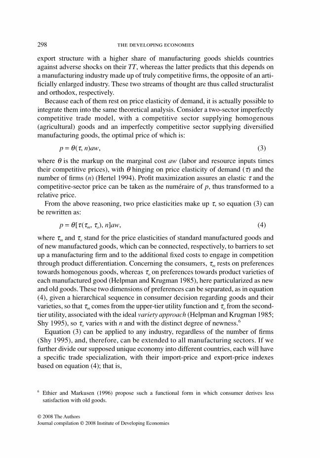
The equation (7) for TT changes then assumes the following empirical form:

TTi = β1MERi + β2REMi + εi, (10)

where the coefficients β1 and β2 express the contribution of each source of export-price elasticities on TTi change, defined in the previous section, which substitutesTT j. Notice that MER is the reciprocal of the commodities export ratio, so its impactis considered therein. Another feature of equation (10) is that the empirical contentof the two independent variables, as defined in equations (8) and (9), is such thatβ1 gives the export-price impact of manufacturing goods controlled for theircompetitiveness, REM.

Accounting for this endogenous TT, the previous debt-crisis model evolves to:

TTi = β1MERi + β2REMi + ε1i, (11a)

(11b)

Matrix X3 stands for those exogenous variables intended to express bad stabiliza-tion policies, defined above, whereas ε1i and ε2i stand for the random errors. System(11) defines how microeconomic distortions (REM) and economic structure (MER)determine the chance of a country going through crisis (RESCH), given externalvicissitudes such as those of the early 1980s.

Should trade policy-induced resource misallocation explain TT variations andultimately the crisis, then a question comes immediately to mind: what preventedcountries from changing these nonoptimal policies? Conflicts between heterogeneousagents around sharing the costs and benefits of policy changes can, as withstabilization policies, delay reforms in trade policies (Alesina and Drazen 1991;Alesina 1994). Hence, social cleavages and institutional strength can equally helpto explain procrastination in enacting policies promoting more efficient resourceallocation.

9 An example is the OPEN index by Sachs and Warner (1995). We do not consider total trade flows[(exports + imports)/GDP] as an alternative variable because both flows are structurally affected bythe countries’ sizes and they do not measure distortion.

RESCH TTi i i .= + ′ +γ β ε1 3 3 2X



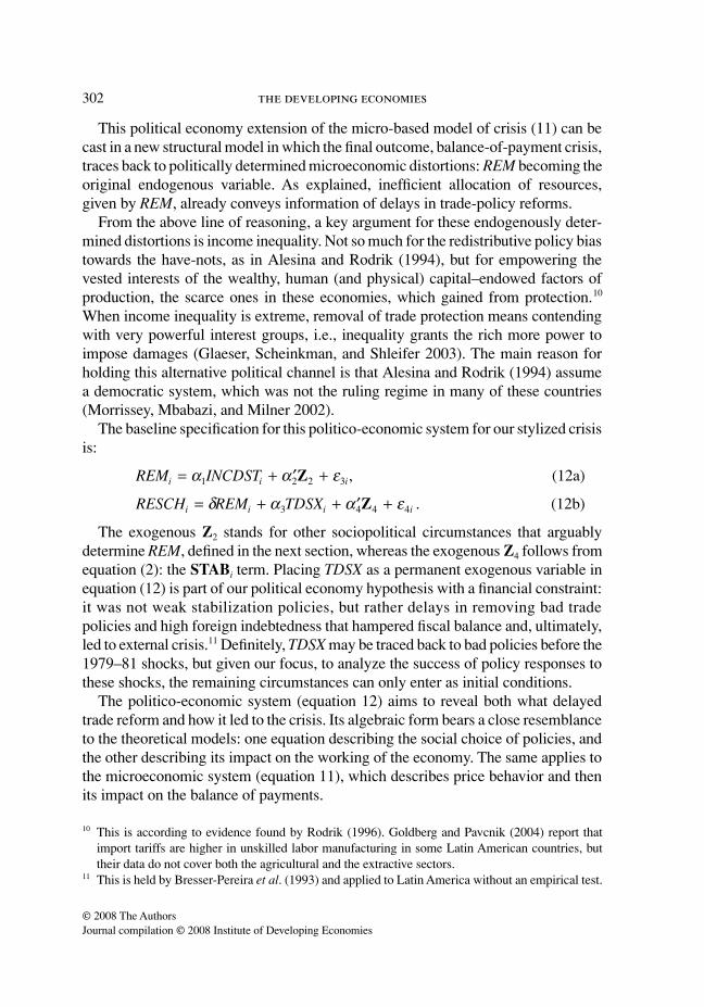
This political economy extension of the micro-based model of crisis (11) can becast in a new structural model in which the final outcome, balance-of-payment crisis,traces back to politically determined microeconomic distortions: REM becoming theoriginal endogenous variable. As explained, inefficient allocation of resources,given by REM, already conveys information of delays in trade-policy reforms.

From the above line of reasoning, a key argument for these endogenously deter-mined distortions is income inequality. Not so much for the redistributive policy biastowards the have-nots, as in Alesina and Rodrik (1994), but for empowering thevested interests of the wealthy, human (and physical) capital–endowed factors ofproduction, the scarce ones in these economies, which gained from protection.10

When income inequality is extreme, removal of trade protection means contendingwith very powerful interest groups, i.e., inequality grants the rich more power toimpose damages (Glaeser, Scheinkman, and Shleifer 2003). The main reason forholding this alternative political channel is that Alesina and Rodrik (1994) assumea democratic system, which was not the ruling regime in many of these countries(Morrissey, Mbabazi, and Milner 2002).

The baseline specification for this politico-economic system for our stylized crisisis:

(12a)

(12b)

The exogenous Z2 stands for other sociopolitical circumstances that arguablydetermine REM, defined in the next section, whereas the exogenous Z4 follows fromequation (2): the STABi term. Placing TDSX as a permanent exogenous variable inequation (12) is part of our political economy hypothesis with a financial constraint:it was not weak stabilization policies, but rather delays in removing bad tradepolicies and high foreign indebtedness that hampered fiscal balance and, ultimately,led to external crisis.11 Definitely, TDSX may be traced back to bad policies before the1979–81 shocks, but given our focus, to analyze the success of policy responses tothese shocks, the remaining circumstances can only enter as initial conditions.

The politico-economic system (equation 12) aims to reveal both what delayedtrade reform and how it led to the crisis. Its algebraic form bears a close resemblanceto the theoretical models: one equation describing the social choice of policies, andthe other describing its impact on the working of the economy. The same applies tothe microeconomic system (equation 11), which describes price behavior and thenits impact on the balance of payments.

10 This is according to evidence found by Rodrik (1996). Goldberg and Pavcnik (2004) report thatimport tariffs are higher in unskilled labor manufacturing in some Latin American countries, buttheir data do not cover both the agricultural and the extractive sectors.

11 This is held by Bresser-Pereira et al. (1993) and applied to Latin America without an empirical test.

REM INCDSTi i i ,= + ′ +α α ε1 2 2 3Z

RESCH REM TDSXi i i i .= + + ′ +δ α α ε3 4 4 4Z



IV. ESTIMATING THE STRUCTURAL MODELS

The simultaneous equation systems (11) and (12) can be represented by the follow-ing two structural equations:

(13a)

(13b)

where y1 and y2 are the endogenous variables, X1 and X2 the exogenous variables andε1i and ε2i the error terms, assumed to be normally distributed. The system is recur-sive in that the first endogenous variable is completely determined by exogenousones and then, given y1i, y2i is likewise determined (Greene 2000).

To estimate the above equations, we choose the maximum likelihood structuralequation model (SEM) technique, an advantage of which is that it can be used toestimate models with an endogenous binary variable in a system space spanned bya small sample; the case here. The fundamental hypothesis of SEM is: given the setof model parameters θ = (β, γ ), then Σ(θ) = Σ(θ*), where Σ(θ) is the covariancematrix of the observed variables and Σ(θ*) is the covariance matrix written as afunction of the estimated parameters. This means that we can choose the parametersin Σ(θ*) to make it as close as possible to the observed sample covariance matrixΣ(θ), presented as Appendix Table 1, maximizing the use of available empiricalinformation.12

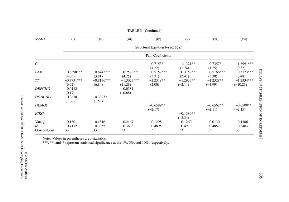
Estimates of the microeconomic-based model (equation 11) of foreign debtdefault are shown in Table 3, with the equation for the endogenous TT in the upperpanel and the one for RESCH in the lower one. Columns (i) to (iii) refer to variantsof the RESCH equation, which test the DIRECT evidence of bad stabilizationpolicies, whereas the remaining variants test variations in the SOCPOL variables.

As shown by the z-statistics of the upper-panel model, from columns (i) to (vi),manufacturing efficiency (REM) and export ratio (MER) do explain TT changes inthe early 1980s, and, as shown in the lower panel, the endogenous TT helps toexplain the crisis. Hence, allocation distortion in the manufacturing industry, bycontributing to the downward changes in the relative export prices, helps to explainwhich country went through the crisis.

Models (i)–(iii) show that none of the direct evidence of delayed stabilizationpolicies is statistically significant in explaining RESCH, contradicting the previoussingle regression estimates. Note that the new model has greater accuracy in at leasttwo ways: (1) data on allocation distortions as given by REM is more reliablethan that in OPEN, as explained before, and (2) it is the only model specifying the

12 Detailed considerations about different structural systems can be found in Hoyle (1995) and Kline(2005).

y i1 1 1 1 ,= ′ +β εX

y yi i2 1 1 2 2 2 ,= + ′ +γ β εX

304th

e developing econ

omies

© 2008 T

he Authors



conomies

TABLE 3

Estimates of the Microeconomic Structural Model of Crisis

Model (i) (ii) (iii) (iv) (v) (vi) (vii)

Structural Equation for TT

Path Coefficients

C 0.8011*** 0.8011*** 0.8011*** 0.8011**** 0.8011*** 0.7933***(25.23) (25.23) (25.23) (25.23) (25.23) (22.99)

MER −0.2646** −0.2646** −0.2646** −0.2646** −0.2646** −0.183 1.2305***(−1.87) (−1.87) (−1.87) (−1.87) (−1.87 ) (−1.18) (5.92)

REM 0.1284*** 0.1284*** 0.1284*** 0.1284*** 0.1284*** 0.1064***(3.43) (3.43) (3.43) (3.43) (3.43) (2.63)

OPEN 0.11 1.2852***(1.26) (4.51)

Var(ε1) 0.0083 0.0084 0.0084 0.0084 0.0084 0.0078 0.1709R2 0.4226 0.4225 0.4225 0.4224 0.4228 0.4569 0.5060

delays in stabilization

or in reform

s?305

© 2008 T

he Authors



conomies

Structural Equation for RESCH

Path Coefficients

C 0.7153* 1.1321** 0.7357* 1.6991***(1.22) (1.74) (1.25) (9.32)

LAM 0.6398*** 0.6442*** 0.7576*** 0.5157*** 0.3752*** 0.5166*** 0.5173***(4.05) (3.81) (4.25) (3.31) (2.41) (3.30) (3.48)

TT −0.7731*** −0.8136*** −1.3023*** −1.2318** −1.2933** −1.2328** −1.2334***(6.02) (6.84) (11.28) (2.00) (−2.14) (−1.99) (−10.21)

DEFCHG 0.0112 −0.0381(0.17) (−0.68)

DODCHG 0.3638 0.3393*(1.36) (1.59)

DEMOC −0.6589** −0.6562** −0.6500**(−2.17) (−2.11) (−2.15)

ICRG −0.1380**(−2.34)

Var(ε2) 0.1801 0.1816 0.2167 0.1298 0.1260 0.0130 0.1306R2 0.4112 0.3955 0.3678 0.4895 0.4976 0.4852 0.8403Observations 33 33 33 33 33 33 33

Note: Values in parentheses are t-statistics.***, **, and * represent statistical significance at the 1%, 5%, and 10%, respectively.

Model (i) (ii) (iii) (iv) (v) (vi) (vii)

TABLE 3 (Continued)



microeconomic relationship (i.e., how allocation inefficiency affects prices).Regarding the SOCPOL variables, DEMOC and ICRG are statistically significantfor explaining RESCH, with their negative sign showing that weak institutionscontributed to the crisis. However, we cannot pinpoint whether they contributed to thecrisis through disputes delaying stabilization policies, or through microeconomicincentives related to property rights. The same applies to LAM (the Latin Americadummy).

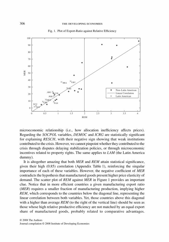
It is altogether amazing that both MER and REM attain statistical significance,given their high (0.85) correlation (Appendix Table 1), reinforcing the singularimportance of each of these variables. However, the negative coefficient of MERcontradicts the hypothesis that manufactured goods present higher price elasticity ofdemand. The scatter plot of REM against MER in Figure 1 provides an importantclue. Notice that in more efficient countries a given manufacturing export ratio(MER) requires a smaller fraction of manufacturing production, implying higherREM, which corresponds to the countries below the diagonal line, representing thelinear correlation between both variables. Yet, those countries above this diagonalwith a higher than average REM (to the right of the vertical line) should be seen asthose whose high relative productive efficiency are not matched by an equal exportshare of manufactured goods, probably related to comparative advantages.

Fig. 1. Plot of Export-Ratio against Relative Efficiency



However, the upper-left quadrant gathers the most inefficient countries, where above-diagonal points match very low allocative efficiency (REM). Curiously enough, allLatin American countries, the most enthusiastic practitioners of import-substitutionstrategy at that time, fall inside this quadrant, except Panama. Given that most LatinAmerican countries experienced large TT losses, this explains the negative coefficientof MER and TT: the above diagonal points, controlled for REM, stand for artificiallydriven manufacturing exports, producing old-fashioned or less-preferred goods.

Hence, the view that the fall in TT preceding the debt crisis is basically result ofa commodity price movement does not hold true: our cross-country analysis showsthat it is also explained by inefficient industrialization. Decisive proof for this isgiven by a model where endogenous TT is determined only by MER and OPEN(column vii of Table 3): MER becomes positive, maintaining its significance, whileOPEN recovers its statistical significance, which also reinforces the SEM’s modelas compared to the single regression model of the previous section. Reinserting REM(column vi), MER shifts to negative again and OPEN becomes nonsignificant.

The above results compel us to estimate the politico-economic system (equation12) of the crisis caused by delayed reforms, the results of which are shown in Table 4below. The above analysis also entitles us to place the Latin American dummy(LAM) as the Z2 variable determining bad trade policy (REM), with LAM standingfor ideology: representing the continent’s strong belief in protectionism. In the firstthree columns, we test the vector DIRECT (direct evidence of bad stabilizationpolicies) while in the remaining columns we test the alternative SOCPOL variables.

As predicted, both INCDSTR and LAM affect REM negatively, and thisendogenous variable in turn affects RESCH negatively: first line of the lower panel.Therefore, both income inequality and Latin America’s trade policy orientationexplain, first, REM, persisting distortions or delayed trade-policy reforms and,ultimately, the debt crisis. This finding, together with the graphical analysis, dis-misses the supposition that LAM simply conveys financial contagion in the region.Part of the contribution of LAM to REM might reflect the low skilled-labor formationin this region (see Ranis and Stewart 2001), reducing the relative efficiency inmanufacturing industries for the same bad incentives to industrialization.

The relevance of income inequality did not show up in the one-equation model forthe crisis in Section II.13 It might be questioned that the impact of INCDST is relatedto an endogenous growth process, as surveyed in Aghion and Williamson (1999),rather than the claimed political relationship. However, the dependent variable,REM, stands for distortion in resource allocations rather than growth performance.

Foreign debt services (TDSX) are also significant in all structural equations forRESCH (second line in the lower panel of Table 4), with the predicted sign. In

13 Without missing the likely role of restricting the sample to a set of developing countries.



contrast, none of the DIRECT evidence of bad stabilization policies attains statisticalsignificance, as in the previous system. This corroborates the proposed politico-economic thesis that it was not weak fiscal policies, but delays in removing theimport-substitution strategy, further constrained by high foreign indebtedness, thatled to the external crisis.

TABLE 4

Estimates of the Politico-Economic Structural Model of Crisis

Model (i) (ii) (iii) (iv) (v)

Structural Equation for REM

Path Coefficients

C 2.4211*** 2.4213*** 2.4208*** 2.4131*** 2.4216***(8.20) (8.35) (8.35) (8.30) (8.17)

INCDSTR −0.0354** −0.0381** −0.0381** −0.0378** −0.0382**(−1.91) (−1.94) (−1.94) (−1.91) (−1.89)

LAM −0.8699*** −0.8699*** 0.8698*** −0.8682*** −0.8700***(−2.30) (−2.34) (−2.34) (−2.33) (−2.29)

Var(ε 1) 0.6371 0.6381 0.6372 0.6387 0.6401R2 0.4113 0.4112 0.4114 0.4087 0.4105

Structural Equation for RESCH

Path Coefficients

REM −0.2125*** −0.1921*** −0.2279*** −0.1219 −0.1047***(−4.39) (−4.32) (−4.82) (−2.25) (−1.64)

TDSX 0.0183*** 0.0214*** 0.0168*** 0.0291*** 0.0293***(3.41) (4.43) (3.14) (5.22) (5.01)

DEFCHG −0.0354 −0.0543***(−0.67) (−1.30)

DODCHG 0.1223 0.1886(0.59) (1.11)

DEMOC −0.1502(−0.68)

ICRG −0.0747**(−1.94)

SOCIAL 0.1461**(1.86)

Var(ε2) 0.1261 0.1241 0.1320 0.1369 0.1095R2 0.4936 0.4997 0.4747 0.4436 0.5502Observations 33 33 33 33 33

Note: Values in parentheses are t-statistics.***, **, and * represent statistical significance at the 1%, 5%, and 10% level, respectively.



Neither DEMOC nor the remaining SOCPOL variables (not reported to avoidredundancy) are statistically significant for explaining RESCH, except ICRG andSOCIAL (public spending on social insurance) in a model having none of theDIRECT variables (see the bottom lines of model (v)). However, the positive sign ofSOCIAL shows that it reinforces the crisis, contradicting Rodriks’ (1999a) hypothesisof delayed stabilization. Besides, we cannot tell whether or not ICRG does not stand,instead, for property-rights problems.

An inexorable question that arises from the above findings is why delays instabilization policies were less of a problem than delays in trade reforms? A crucialreason is that the latter are known to have a large impact on income redistribution,relative to the net aggregate gain to society (Rodrik 1994), which means that thecost–benefit ratio is considered too high by politicians planning to carry suchreforms. This is bound to be more troublesome in extremely unequal societies,where the differential power of interest groups reinforces the political delays.

V. CONCLUSIONS

External economic problems (TT shocks and foreign indebtedness) statisticallyexplain which countries plunged into the 1980s’ debt crisis, so that the hypothesisof bad stabilization policies cannot be invoked to explain the observed large diver-gence in macroeconomic performance among these developing countries. Weattained this result, opposed to those found in some recent and influential papers, byapproaching the case as a specific balance-of-payment crisis, rather than a standardgrowth deviation, which implied new measures of both shocks and indebtedness,and the redefinition of the relevant countries.

Most importantly, our model of external shocks leading to a crisis, under extrememicroeconomic distortions, confirmed that resource misallocations towards the manu-facturing industry explain TT changes that then help to predict foreign debt default.Its political economy extension, in turn, showed that both income inequality andLatin American trade-policy orientation explain these allocation distortions, whicheventually, together with foreign indebtedness, explain the onset of the crisis. Thefindings relating to Latin American countries add to previous studies on economicgrowth, highlighting problems related to allocation distortions. To sum up, the newpicture we obtain about the 1980s’ crisis is of embattled governments dealing withoverwhelming external difficulties, hardly manageable by good fiscal and monetarypolicies, although avoidable had the microeconomic distortions been smaller.

Only by means of SEM could we trace how external shocks led to a balance-of-payment crisis under allocative inefficiency. Likewise, this sequential analysisenabled us to uncover the relevance of income inequality to bad macroeconomicperformance: tracing a path from the sources of microeconomic distortions to theirimpact on external payments.



REFERENCES

Aghion, Philippe, and Jeffrey G. Williamson. 1999. Growth, Inequality and Globalization:Theory, History and Policy. Cambridge: Cambridge University Press.

Alesina, Alberto. 1994. “Political Models of Macroeconomic Policy and Fiscal Reforms.” InVoting for Reform, ed. S. Haggard and S. Webb. Oxford: Oxford University Press.

Alesina, Alberto, and Allan Drazen. 1991. “Why Are Stabilizations Delayed?” AmericanEconomic Review 81, no. 5: 1170–88.

Alesina, Alberto, and Dani Rodrik. 1994. “Distributive Politics and Economic Growth.”Quarterly Journal of Economics 109, no. 2: 465–90.

Alesina, Alberto, and Roberto Perotti. 1994. “The Political Economy of Growth: A CriticalSurvey of the Recent Literature.” World Bank Economic Review 8, no. 3: 351–71.

Barro, Robert J. 1991. “Economic Growth in a Cross Section of Countries.” Quarterly Jour-nal of Economics 106, no. 2: 407–43.

Barro, Robert J., and Jong-Wha Lee. 1994. “Data Set for a Panel of 138 Countries.” Techni-cal Report, National Bureau of Economic Research.

Berg, Andrew, and Jeffrey Sachs. 1988. “The Debt Crisis: Structural Explanation of CountryPerformance.” Journal of Development Economics 29, no. 3: 271–306.

Bresser-Pereira, Luiz Carlos; Jose Maria Maravall; and Adam Przeworski. 1993. EconomicReforms in New Democracies. Cambridge: Cambridge University Press.

Bruton, Henri. 1998. “A Reconsideration of Import Substitution.” Journal of Economic Lit-erature 36 no. 2: 903–96.

Cinquetti, Carlos A. 2005. “The Debt Crisis: A Re-Appraisal.” Brazilian Journal of PoliticalEconomy 25, no. 3: 1–12.

Cline, William. 1984. International Debt: Systemic Risk and Policy Response. Cambridge,Mass.: MIT Press.

Cristini, Annalasia. 1995. “Economic Activity and Commodity Prices: Theory and Evi-dence.” In North-South Linkages and International Macroeconomic Policy, ed. DavidVines and David Currie. Cambridge: Cambridge University Press.

Easterly, William; Michael Kremer; Lant Pritchett; and Lawrence H. Summers. 1993. “GoodPolicy or Good Luck? Country Growth Performance and Temporary Shocks.” Journalof Monetary Economics 32, no. 3: 459–83.

Easterly, William, and Ross Levine. 1996. “Africa’s Growth Tragedy: Policies and EthnicDivisions.” Quarterly Journal of Economics 112, no. 4: 1203–50. Dataset: http://www.nyu.edu\fas\institute/dr/Easterly/Research.html (Accessed December 15 2005).

Economic Commission for Africa (ECA). 1984–1986. African Statistical Yearbook. AddisAbaba: ECA.

Economic Commission for Latin America and the Caribbean (ECLAC). 1982 and 1986.Economic Survey of Latin America and the Caribbean. Santiago: ECLAC.

Economic and Social Commission for Asia and the Pacific (ESCAP). 1986. StatisticalYearbook for Asia and the Pacific. Bangkok: ESCAP.

Ethier, Wilfred J., and James R. Markusen. 1996. “Multinational Firms, Technology Diffu-sion and Trade.” Journal of International Economics 41, nos. 1–2: 1–28.

Fisher, Stanley. 2002. “What I Learned at the IMF.” Newsweek International, December2001–February 2002: 86–87.

Fratzscher, Marcel. 1998. “Why Are Currency Crises Contagious? A Comparison of theLatin American Crisis of 1994–1995 and the Asian Crisis of 1997–1998.” Weltwirt-schaftliches Archiv 134, no. 4: 664–91.

http://www.nyu.edu\fas\institute/dr/Easterly/Research.html



Glaeser, Edward; Jose A. Scheinkman; and Andrei Shleifer. 2003. “The Injustice of Inequal-ity.” Journal of Monetary Economics 50, no. 1: 199–222.

Goldberg, Pinelopi K., and Nina Pavcnik. 2004. Trade, Inequality, and Poverty: What Do WeKnow? Cambridge, Mass.: National Bureau of Economic Research.

Greene, William H. 2000. Econometric Analysis. Upper Saddle River, N.J.: Prentice-Hall.Helpman, Elhanan, and Paul R. Krugman. 1985. Market Structure and Foreign Trade. Cam-

bridge, Mass.: MIT Press.———. 1989. Trade Policy and Market Structure. Cambridge, Mass.: MIT Press.Hertel, Thomas W. 1994. “The ‘Procompetitive’ Effects of Trade Policy Reform in a Small,

Open Economy.” Journal of International Economics 36, nos. 3–4: 391–411.Hoyle, Rick. 1995. Structural Equation Modeling: Concepts, Issues and Applications. Thou-

sand Oaks: Sage Publications.International Monetary Fund (IMF). 1989 and 1993. International Financial Statistics Year-

book. Washington, D.C.: IMF.Kline, Rex B. 2005. Principles and Practice of Structural Equation Modeling. 2nd ed. New

York: Guilford Press.Krueger, Anne O. 1995. Trade Policies and Developing Nations. Integrating National

Economies: Promise and Pitfalls. Washington, D.C.: Brookings Institution Press.Labys, Walter C.; Eugene Kouassi; and Michel Terraza. 2000. “Short-Term Cycles in

Primary Commodity Prices.” Developing Economies 38, no. 3: 330–42.Little, Ian M. D.; Richard N. Cooper; and Warner Max Corden. 1994. Boom, Crisis, and

Adjustment. New York: Oxford University Press.Minsky, Hyman. 1977. “A Theory of Systemic Fragility.” In Financial Crises: Institutions

and Markets in a Fragile Environment, ed. Edward I. Altman and Arnold W. Sametz.New York: Wiley.

Morrissey, Oliver; Jennifer Mbabazi; and Chris Milner. 2002. “Inequality, Trade Liberalisa-tion and Growth.” CSGR Working Paper 102, no. 2.

Ranis, Gustav, and Frances Stewart. 2001. “Growth and Human Development: ComparativeLatin American Experience.” Developing Economies 39, no. 4: 333–65.

Republic of China. 1993. Taiwan Statistical Data Book. Taipei: Council for EconomicPlanning and Development.

Riedel, James, and P. Athukorala. 1995. Export Growth and the Terms of Trade: The Case ofCurious Elasticities. Cambridge: Cambridge University Press.

Rodriguez, Fernando, and Dani Rodrik. 2001. “Trade Policy and Economic Growth: A Skeptic’sGuide to the Cross-National Evidence.” In Macroeconomics Annual 2000, ed. BenBernanke and Kenneth Rogoff. Cambridge, Mass.: MIT Press for NBER.

Rodrik, Dani. 1994. “The Rush to Free Trade in the Developing World: Why So Late? WhyNow? Will It Last?” In Voting for Reform: Democracy, Political Liberalization, andEconomic Adjustment, ed. Stephan Haggard and Steven Webb. New York: OxfordUniversity Press.

———. 1996. “Understanding Economic Policy Reform.” Journal of Economic Literature34, no. 1: 9–41.

———. 1999a. The New Global Economy and Developing Countries: Making OpennessWork. Washington, D.C.: Overseas Development Council.

———. 1999b. “Where Did the Growth Go? External Shocks, Social Conflict, and GrowthCollapses.” Journal of Economic Growth 4, no. 4: 385–412.

Sachs, Jeffrey, and Andrew Warner. 1995. “Economic Reform and the Process of GlobalIntegration.” Brooking Papers on Economic Activity 1: 1–118.



Shy, Oz. 1995. Industrial Organization: Theory and Applications. Cambridge, Mass.: MITPress.

Taylor, Lance. 1991. Income Distribution, Inflation and Growth: Lectures on StructuralistMacroeconomic Theory. Cambridge, Mass.: MIT Press.

Tobin, James. 1980. Asset Accumulation and Economic Activity. Chicago: University ofChicago Press.

United Nations Conference on Trade and Development (UNCTAD). 2000. Handbook ofInternational Trade and Development Statistics. Geneva: UNCTAD.

World Bank. 1982. World Development Report. Washington D.C.: World Bank.———. 1987 and 1995. World Tables. Washington D.C.: World Bank.———. 1998 and 2000. World Development Indicators. Washington D.C.: World Bank.



APPENDIX

DATA SOURCES

DEFCH and PRCHG: IMF, International Financial Statistics Yearbook, 1993(Washington, D.C.: IMF).

DEMOC: Freedom House via Dani Rodrik’s data bank, kindly provided to theauthors.

DODCHG: World Bank, World Tables, 1987 and 1995 (Washington, D.C.: WorldBank).

ICRG: International Country Risk Guide via Rodrik (idem).INCDSTR: Several sources as quoted in Berg and Sachs (1988).LAW: Easterly and Levine (1996) via Rodrik (idem).MER and REM: World Bank, World Development Indicators, 1998 (Washington,

D.C.: World Bank, 2000) and UNCTAD, Handbook of International Trade andDevelopment Statistics, 2000 (Geneva: United Nations Conference on Trade andDevelopment).

OPEN: UNCTAD via Barro and Lee (1994).RESCH: World Bank via Berg and Sachs (1988).SOCIAL: Rodrik (idem).TDSX: World Bank, World Tables, 1987 and 1995 (Washington, D.C.: World Bank)

and World Bank, World Development Report, 1982 (Washington, D.C.: WorldBank).

TT: Republic of China, Taiwan Statistical Data Book, 1993 (Taipei: Council forEconomic Planning and Development, Republic of China); ESCAP, StatisticalYearbook for Asia and the Pacific, 1986 (Bangkok: Economic and Social Com-mission for Asia and the Pacific); ECLAC, Economic Survey of Latin Americaand the Caribbean, 1982 and 1986 (Santiago: Economic Commission for LatinAmerica and the Caribbean); ECA, African Statistical Yearbook, 1984–1986(Addis Ababa: Economic Commission for Africa); IMF, International FinancialStatistics: Supplement on Trade Statistics, 1988 and Yearbook, 1989 (Washing-ton, D.C.: IMF).

314th

e developing econ

omies

© 2008 T

he Authors



conomies

APPENDIX TABLE 1

Partial Correlations between Independent Variables

LAM TT TDSX DEFCHG PRCHG DODCHG OPEN INCDSTR SOCIAL LAW ICRG DEMOC MER

TT −0.45 1.00TDSX 0.46 −0.29 1.00DEFCHG −0.19 0.10 −0.17 1.00PRCHG 0.33 −0.08 0.21 −0.59 1.00DODCHG 0.30 −0.26 0.06 −0.62 0.78 1.00OPEN 0.00 0.42 −0.06 0.04 −0.07 −0.18 1.00INCDSTR 0.50 −0.39 0.52 0.05 0.17 −0.02 0.09 1.00SOCIAL 0.20 −0.06 −0.23 −0.09 −0.21 −0.03 −0.06 −0.27 1.00LAW 0.13 −0.01 −0.12 −0.37 0.23 0.30 −0.04 −0.28 0.37 1.00ICRG −0.14 −0.04 −0.20 −0.06 −0.09 −0.02 −0.21 −0.18 0.08 0.44 1.00DEMOC 0.25 −0.17 −0.15 −0.24 0.39 0.47 0.21 0.05 0.03 0.11 0.09 1.00MER −0.45 0.39 −0.11 −0.01 −0.12 −0.11 0.09 −0.41 0.16 0.48 0.45 −0.21 1.00REM −0.59 0.62 −0.18 0.00 −0.11 −0.15 0.30 −0.45 −0.14 0.27 0.25 −0.12 0.85

The debt crisis: a re-appraisal

Documents

Transcript of The debt crisis: a re-appraisal