General Disequilibrium Analysis with Inside Debt

Abstract

This paper incorporates inside nominal debt into a Keynesian general disequilibrium model. It shows how nominal wage adjustment may be insufficient to restore Walrasian equilibrium. Nominal wage reductions lower aggregate demand by increasing debt service burdens. This aggravates Keynesian deficient demand unemployment. When there is classical unemployment, falling nominal wages mean that the economy may hit a Keynesian constraint before it attains Walrasian full employment. In situations of repressed inflation, rising nominal wages reduce debt service burdens and increase aggregate demand, thereby worsening the extent of excess demand. JEL ref.: E0, E1 Key words: General disequilibrium, inside debt, nominal wage flexibility.

Final Revision, March 1998.

Thomas I. Palley

Assistant Director of Public Policy, AFL-CIO 815 Sixteenth Street

Washington, D.C. 20006 The detailed comments of an anonymous referee are deeply appreciated, and they have greatly improved the paper. Remaining errors are my own.

11 Introduction Inside debt is a notable feature of economies with developed financial systems, and

Irving Fisher (1933) emphasized its importance in his debt - deflation theory of economic

depressions. The existence of inside debt means that nominal wage reductions can have a

negative effect on aggregate demand and therefore be destabilizing with regard to the

problem of unemployment.

The argument is as follows. If worker households are debtors, nominal wage

reductions will increase the burden of their debts and reduce their consumption spending.

To the extent that nominal wage reductions lower prices, creditors will be made better off

and they will increase their spending. However, aggregate demand can fall in response to

lower nominal wages if (i) the marginal propensity to spend of debtors exceeds that of

creditors, and (ii) this net negative debt effect swamps the Pigou effect.

The importance of inside debt has been evident in recent economic experience. The

extended sluggishness of the recovery following the last U.S. recession has been

attributed to the build up of debt which needed to be worked off before a sustained

recovery could begin. Another instance is the U.K.'s withdrawal from the European

exchange rate mechanism in 1992. The British government needed to increase interest

rates to support Sterling, but it was unable to do so because of the potential negative

aggregate demand impact arising from massive levels of mortgage debt. In this instance,

higher interest rates rather than lower prices and nominal wages would have effected an

adverse transfer between debtors and creditors.

Despite its potential significance, inside debt is absent in most macroeconomic

analyses. The current paper seeks to fit considerations of inside debt into a general

2disequilibrium analysis of the type pioneered by Barro and Grossman (1971) and by

Malinvaud (1977). Such a treatment illuminates the difficulties for macroeconomic

adjustment posed by the existence of inside debt.

2 Micro foundations of the Fisher debt effect

Before beginning the macroeconomic analysis, it is worth exploring the

microeconomic foundations of the Fisher debt effect. One argument rests on

psychological disposition: debtors are psychologically more optimistic than creditors and

have a higher marginal propensity to consume (MPC). A second argument rests on

liquidity constraints: debtor households are liquidity constrained and have a MPC of

unity. A third argument is based on the conventional short run Keynesian consumption

function, according to which the MPC falls with income. If on average debtor households

have lower incomes than creditor households, then the MPC of debtor households will

tend to be higher than that of creditors. A fourth argument is based on rule of thumb

saving behavior, whereby households separate wage income from other types of income,

and finance consumption out of wage income while saving more out of profit and interest

income. In this case, debtors will have a larger propensity to consume than creditors,

since the latter will treat interest payments as part of non-wage income.

Institutional developments associated with the proliferation of indirect credit markets

may also have made the Fisher debt effect more important. With direct credit markets, the

Fisher debt effect operates directly on the transfer of income from debtors to creditors.

With indirect credit markets there is a double filter that magnifies the effect. In the first

instance, debtors feel the adverse effect of increased real debt burdens. However, debt

service is now paid over to a financial intermediary, and the intermediary likely only pays

3out a fraction of the real debt service windfall as dividends. As a result, the real income

of creditor households does not increase by the same absolute amount as the decline in

debtors' real incomes. This serves to compound the Fisher debt effect as creditors have a

lower MPC and receive a smaller absolute increment in income.

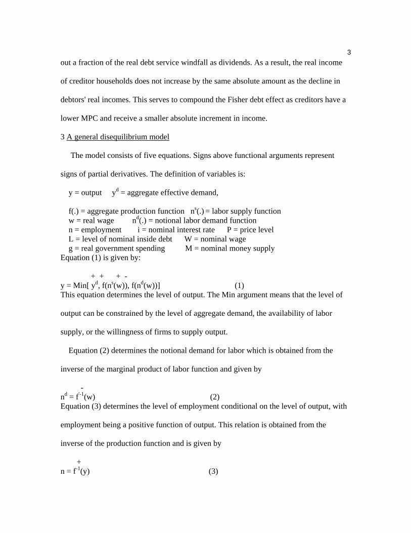
3 A general disequilibrium model

The model consists of five equations. Signs above functional arguments represent

signs of partial derivatives. The definition of variables is:

y = output yd = aggregate effective demand,

f(.) = aggregate production function ns(.) = labor supply function w = real wage nd(.) = notional labor demand function n = employment i = nominal interest rate P = price level L = level of nominal inside debt W = nominal wage g = real government spending M = nominal money supply Equation (1) is given by:

+ + + - y = Min[ yd, f(ns(w)), f(nd(w))] (1) This equation determines the level of output. The Min argument means that the level of

output can be constrained by the level of aggregate demand, the availability of labor

supply, or the willingness of firms to supply output.

Equation (2) determines the notional demand for labor which is obtained from the

inverse of the marginal product of labor function and given by

- nd = f'-1(w) (2) Equation (3) determines the level of employment conditional on the level of output, with

employment being a positive function of output. This relation is obtained from the

inverse of the production function and is given by

+ n = f-1(y) (3)

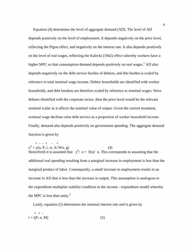
4 Equation (4) determines the level of aggregate demand (AD). The level of AD

depends positively on the level of employment. It depends negatively on the price level,

reflecting the Pigou effect, and negatively on the interest rate. It also depends positively

on the level of real wages, reflecting the Kalecki (1942) effect whereby workers have a

higher MPC so that consumption demand depends positively on real wages.1 AD also

depends negatively on the debt service burden of debtors, and this burden is scaled by

reference to total nominal wage income. Debtor households are identified with worker

households, and debt burdens are therefore scaled by reference to nominal wages. Were

debtors identified with the corporate sector, then the price level would be the relevant

nominal scalar as it affects the nominal value of output. Given the current treatment,

nominal wage declines raise debt service as a proportion of worker household income.

Finally, demand also depends positively on government spending. The aggregate demand

function is given by

+ - - + - + yd = y(n, P, i, w, iL/Wn, g) (4) Henceforth it is assumed that yd/ n < f(n)/ n. This corresponds to assuming that the

additional real spending resulting from a marginal increase in employment is less than the

marginal product of labor. Consequently, a small increase in employment results in an

increase in AD that is less than the increase in output. This assumption is analogous to

the expenditure multiplier stability condition in the income - expenditure model whereby

the MPC is less than unity.2

Lastly, equation (5) determines the nominal interest rate and is given by

+ + - i = i(P, n, M) (5)

5The nominal interest rate depends positively on the price level and employment. Higher

prices reduce the real money supply which drives up interest rates: this is the Keynes

effect. Higher employment raises income and money demand which increases interest

rates. Substituting (5) into (4) yields

yd = y(n, P, i(P,n,M), w, i(P,n,M)L/Wn, g) (4')

Differentiating with respect to n yields

dyd/dn = y1 + y3i2 + y5[i2L/Wn - iL/Wn2] >< 0

The sign of this expression is ambiguous. Increases in employment directly positively

impact demand, but they also raise interest rates which reduces demand. Henceforth, it is

assumed that employment has a positive effect, reflecting the dominance of the direct AD

effect over the indirect interest rate effect.

Figure 1 provides a graphic analogue of the model illustrating the case of

unconstrained Walrasian equilibrium. The labor market clears with labor supply and

labor demand at the real wage of w* both being equal to the level of employment, n*.

Simultaneously, the goods market clears with the level of output equal to the level of AD.

The triangular region lying above the labor supply schedule and below the labor demand

schedule represents the economically relevant region of the labor market. Actual real

wage - employment outcomes are bounded by this region. Points below and to the right

of the labor supply curve are not feasible as labor supply constrains employment, whereas

points above and to the right of the labor demand curve are not feasible as labor demand

constrains employment.

4 Regimes of disequilibrium

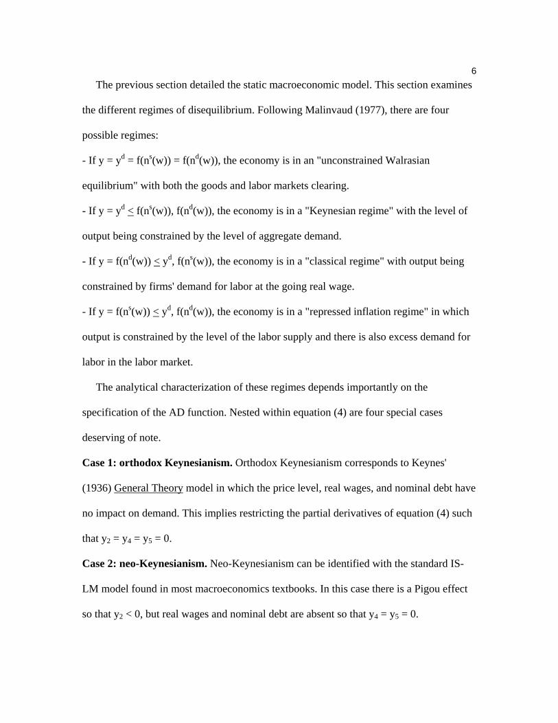
6 The previous section detailed the static macroeconomic model. This section examines

the different regimes of disequilibrium. Following Malinvaud (1977), there are four

possible regimes:

- If y = yd = f(ns(w)) = f(nd(w)), the economy is in an "unconstrained Walrasian

equilibrium" with both the goods and labor markets clearing.

- If y = yd < f(ns(w)), f(nd(w)), the economy is in a "Keynesian regime" with the level of

output being constrained by the level of aggregate demand.

- If y = f(nd(w)) < yd, f(ns(w)), the economy is in a "classical regime" with output being

constrained by firms' demand for labor at the going real wage.

- If y = f(ns(w)) < yd, f(nd(w)), the economy is in a "repressed inflation regime" in which

output is constrained by the level of the labor supply and there is also excess demand for

labor in the labor market.

The analytical characterization of these regimes depends importantly on the

specification of the AD function. Nested within equation (4) are four special cases

deserving of note.

Case 1: orthodox Keynesianism. Orthodox Keynesianism corresponds to Keynes'

(1936) General Theory model in which the price level, real wages, and nominal debt have

no impact on demand. This implies restricting the partial derivatives of equation (4) such

that y2 = y4 = y5 = 0.

Case 2: neo-Keynesianism. Neo-Keynesianism can be identified with the standard IS-

LM model found in most macroeconomics textbooks. In this case there is a Pigou effect

so that y2 < 0, but real wages and nominal debt are absent so that y4 = y5 = 0.

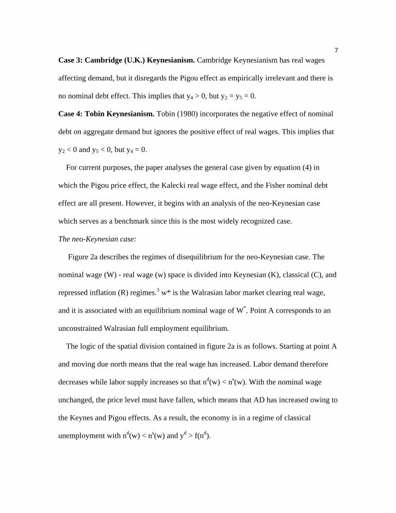
7Case 3: Cambridge (U.K.) Keynesianism. Cambridge Keynesianism has real wages

affecting demand, but it disregards the Pigou effect as empirically irrelevant and there is

no nominal debt effect. This implies that y4 > 0, but y2 = y5 = 0.

Case 4: Tobin Keynesianism. Tobin (1980) incorporates the negative effect of nominal

debt on aggregate demand but ignores the positive effect of real wages. This implies that

y2 < 0 and y5 < 0, but y4 = 0.

For current purposes, the paper analyses the general case given by equation (4) in

which the Pigou price effect, the Kalecki real wage effect, and the Fisher nominal debt

effect are all present. However, it begins with an analysis of the neo-Keynesian case

which serves as a benchmark since this is the most widely recognized case.

The neo-Keynesian case:

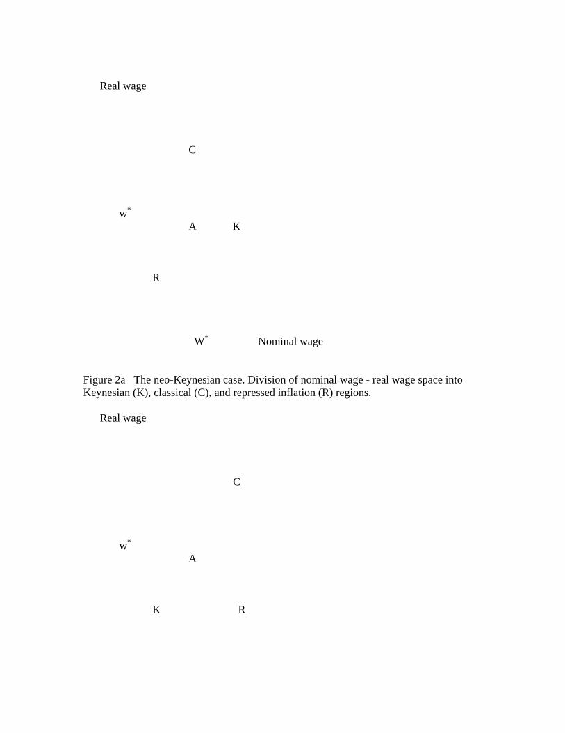
Figure 2a describes the regimes of disequilibrium for the neo-Keynesian case. The

nominal wage (W) - real wage (w) space is divided into Keynesian (K), classical (C), and

repressed inflation (R) regimes.3 w* is the Walrasian labor market clearing real wage,

and it is associated with an equilibrium nominal wage of W*. Point A corresponds to an

unconstrained Walrasian full employment equilibrium.

The logic of the spatial division contained in figure 2a is as follows. Starting at point A

and moving due north means that the real wage has increased. Labor demand therefore

decreases while labor supply increases so that nd(w) < ns(w). With the nominal wage

unchanged, the price level must have fallen, which means that AD has increased owing to

the Keynes and Pigou effects. As a result, the economy is in a regime of classical

unemployment with nd(w) < ns(w) and yd > f(nd).

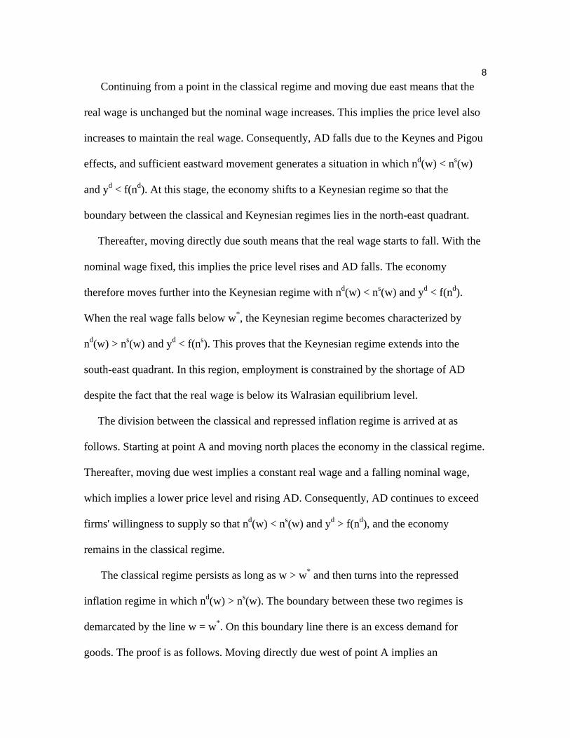
8 Continuing from a point in the classical regime and moving due east means that the

real wage is unchanged but the nominal wage increases. This implies the price level also

increases to maintain the real wage. Consequently, AD falls due to the Keynes and Pigou

effects, and sufficient eastward movement generates a situation in which nd(w) < ns(w)

and yd < f(nd). At this stage, the economy shifts to a Keynesian regime so that the

boundary between the classical and Keynesian regimes lies in the north-east quadrant.

Thereafter, moving directly due south means that the real wage starts to fall. With the

nominal wage fixed, this implies the price level rises and AD falls. The economy

therefore moves further into the Keynesian regime with nd(w) < ns(w) and yd < f(nd).

When the real wage falls below w*, the Keynesian regime becomes characterized by

nd(w) > ns(w) and yd < f(ns). This proves that the Keynesian regime extends into the

south-east quadrant. In this region, employment is constrained by the shortage of AD

despite the fact that the real wage is below its Walrasian equilibrium level.

The division between the classical and repressed inflation regime is arrived at as

follows. Starting at point A and moving north places the economy in the classical regime.

Thereafter, moving due west implies a constant real wage and a falling nominal wage,

which implies a lower price level and rising AD. Consequently, AD continues to exceed

firms' willingness to supply so that nd(w) < ns(w) and yd > f(nd), and the economy

remains in the classical regime.

The classical regime persists as long as w > w* and then turns into the repressed

inflation regime in which nd(w) > ns(w). The boundary between these two regimes is

demarcated by the line w = w*. On this boundary line there is an excess demand for

goods. The proof is as follows. Moving directly due west of point A implies an

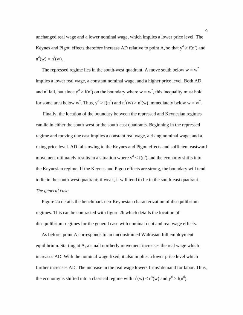
9unchanged real wage and a lower nominal wage, which implies a lower price level. The

Keynes and Pigou effects therefore increase AD relative to point A, so that yd > f(ns) and

nd(w) = ns(w).

The repressed regime lies in the south-west quadrant. A move south below w = w*

implies a lower real wage, a constant nominal wage, and a higher price level. Both AD

and ns fall, but since yd > f(ns) on the boundary where w = w*, this inequality must hold

for some area below w*. Thus, yd > f(nd) and nd(w) > ns(w) immediately below w = w*.

Finally, the location of the boundary between the repressed and Keynesian regimes

can lie in either the south-west or the south-east quadrants. Beginning in the repressed

regime and moving due east implies a constant real wage, a rising nominal wage, and a

rising price level. AD falls owing to the Keynes and Pigou effects and sufficient eastward

movement ultimately results in a situation where yd < f(ns) and the economy shifts into

the Keynesian regime. If the Keynes and Pigou effects are strong, the boundary will tend

to lie in the south-west quadrant; if weak, it will tend to lie in the south-east quadrant.

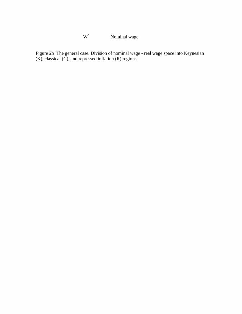
The general case.

Figure 2a details the benchmark neo-Keynesian characterization of disequilibrium

regimes. This can be contrasted with figure 2b which details the location of

disequilibrium regimes for the general case with nominal debt and real wage effects.

As before, point A corresponds to an unconstrained Walrasian full employment

equilibrium. Starting at A, a small northerly movement increases the real wage which

increases AD. With the nominal wage fixed, it also implies a lower price level which

further increases AD. The increase in the real wage lowers firms' demand for labor. Thus,

the economy is shifted into a classical regime with nd(w) < ns(w) and yd > f(nd).

10 Thereafter, moving due east implies a fixed real wage, a rising nominal wage, and a

rising price level. The rising nominal wage is expansionary owing to the Fisher debt

effect; the rising price level is contractionary owing to the Keynes and Pigou effects. If

the Fisher nominal debt effect dominates, then AD increases and the economy remains in

the classical regime.

Turning and moving due south implies that the real wage is falling, the nominal wage

is fixed, and the price level is rising. AD therefore falls. However, the economy remains

in the classical regime as long as w > w*. This is because W > W*, so that with the Fisher

debt effect dominating, AD remains greater than it was at point A so that there is

continuing excess goods demand. Once w falls below w*, then nd(w) > ns(w) and the

economy shifts from the classical regime into the repressed inflation regime.

Moving due west from a point in the repressed regime implies that the real wage is

constant, the nominal wage falls, and the price level also falls. With the Fisher debt effect

dominating the Keynes and Pigou effects, AD falls and sufficient westward movement

places the economy in the Keynesian regime. The exact location of the boundary between

the repressed inflation and Keynesian regimes is unclear. If the Kalecki real wage effect

is strong, then the boundary tends to slope in a south-easterly direction: a higher nominal

wage is needed to offset the negative demand effect of a lower real wage.

Finally, starting from a point in the Keynesian regime and moving north implies that

the real wage is increasing, the nominal wage is constant, and the price level is falling.

This combination means that AD is rising. When w = w*, the economy is still in the

Keynesian regime. This is because W < W*, which means that AD is less than it was at

point A owing to the Fisher debt effect. However, sufficient northerly movement will

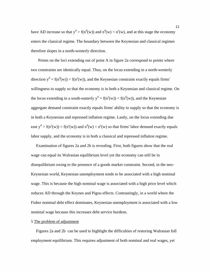
11have AD increase so that yd > f(nd(w)) and nd(w) < ns(w), and at this stage the economy

enters the classical regime. The boundary between the Keynesian and classical regimes

therefore slopes in a north-westerly direction.

Points on the loci extending out of point A in figure 2a correspond to points where

two constraints are identically equal. Thus, on the locus extending in a north-westerly

direction yd = f(nd(w)) < f(ns(w)), and the Keynesian constraint exactly equals firms'

willingness to supply so that the economy is in both a Keynesian and classical regime. On

the locus extending in a south-easterly yd = f(ns(w)) < f(nd(w)), and the Keynesian

aggregate demand constraint exactly equals firms' ability to supply so that the economy is

in both a Keynesian and repressed inflation regime. Lastly, on the locus extending due

east yd > f(ns(w)) = f(ns(w)) and nd(w) = ns(w) so that firms' labor demand exactly equals

labor supply, and the economy is in both a classical and repressed inflation regime.

Examination of figures 2a and 2b is revealing. First, both figures show that the real

wage can equal its Walrasian equilibrium level yet the economy can still be in

disequilibrium owing to the presence of a goods market constraint. Second, in the neo-

Keynesian world, Keynesian unemployment tends to be associated with a high nominal

wage. This is because the high nominal wage is associated with a high price level which

reduces AD through the Keynes and Pigou effects. Contrastingly, in a world where the

Fisher nominal debt effect dominates, Keynesian unemployment is associated with a low

nominal wage because this increases debt service burdens.

5 The problem of adjustment

Figures 2a and 2b can be used to highlight the difficulties of restoring Walrasian full

employment equilibrium. This requires adjustment of both nominal and real wages, yet

12both the Keynesian and classical regions cover diverse spaces in which the directions of

adjustment of nominal and real wages conflict.

Particularly problematic is the fact that resolving Keynesian unemployment when

there is nominal debt can require higher nominal wages, yet this is something labor

markets are unlikely to produce given the existence of unemployment. Similarly,

resolving repressed inflation requires lower nominal wages but this is also something

labor markets are unlikely to produce since there is excess demand for labor.

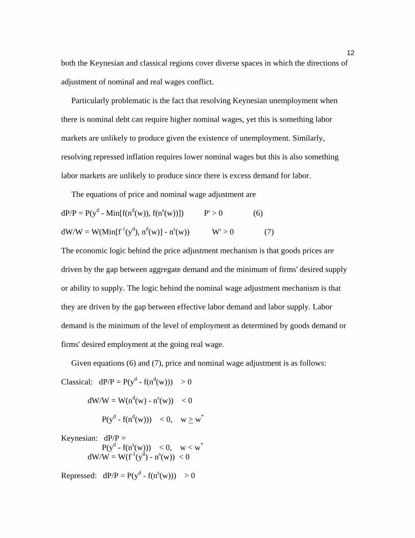
The equations of price and nominal wage adjustment are

dP/P = P(yd - Min[f(nd(w)), f(ns(w))]) P' > 0 (6)

dW/W = W(Min[f-1(yd), nd(w)] - ns(w)) W' > 0 (7)

The economic logic behind the price adjustment mechanism is that goods prices are

driven by the gap between aggregate demand and the minimum of firms' desired supply

or ability to supply. The logic behind the nominal wage adjustment mechanism is that

they are driven by the gap between effective labor demand and labor supply. Labor

demand is the minimum of the level of employment as determined by goods demand or

firms' desired employment at the going real wage.

Given equations (6) and (7), price and nominal wage adjustment is as follows:

Classical: dP/P = P(yd - f(nd(w))) > 0

dW/W = W(nd(w) - ns(w)) < 0

P(yd - f(nd(w))) < 0, w > w*

Keynesian: dP/P = P(yd - f(ns(w))) < 0, w < w* dW/W = W(f-1(yd) - ns(w)) < 0

Repressed: dP/P = P(yd - f(ns(w))) > 0

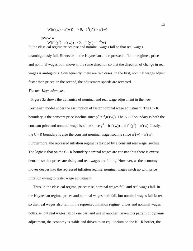
13 W(nd(w) - ns(w)) > 0, f-1(yd) > nd(w)

dW/W = W(f-1(yd) - ns(w)) > 0, f-1(yd) < nd(w) In the classical regime prices rise and nominal wages fall so that real wages

unambiguously fall. However, in the Keynesian and repressed inflation regimes, prices

and nominal wages both move in the same direction so that the direction of change in real

wages is ambiguous. Consequently, there are two cases. In the first, nominal wages adjust

faster than prices: in the second, the adjustment speeds are reversed.

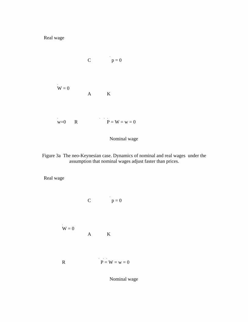
The neo-Keynesian case

Figure 3a shows the dynamics of nominal and real wage adjustment in the neo-

Keynesian model under the assumption of faster nominal wage adjustment. The C - K

boundary is the constant price isocline since yd = f(nd(w)). The K - R boundary is both the

constant price and nominal wage isocline since yd = f(ns(w)) and f-1(yd) = ns(w). Lastly,

the C - R boundary is also the constant nominal wage isocline since nd(w) = ns(w).

Furthermore, the repressed inflation regime is divided by a constant real wage isocline.

The logic is that on the C - R boundary nominal wages are constant but there is excess

demand so that prices are rising and real wages are falling. However, as the economy

moves deeper into the repressed inflation regime, nominal wages catch up with price

inflation owing to faster wage adjustment.

Thus, in the classical regime, prices rise, nominal wages fall, and real wages fall. In

the Keynesian regime, prices and nominal wages both fall, but nominal wages fall faster

so that real wages also fall. In the repressed inflation regime, prices and nominal wages

both rise, but real wages fall in one part and rise in another. Given this pattern of dynamic

adjustment, the economy is stable and driven to an equilibrium on the K - R border, the

14very end point of which includes the Walrasian full employment equilibrium. On this

border there is no unemployment, but firms have vacancies everywhere except the point

of Walrasian equilibrium. In terms of figure 1, the economy settles on the labor supply

schedule below the point of Walrasian full employment equilibrium.

Figure 3b shows the dynamics of adjustment for the neo-Keynesian case when prices

adjust faster. The figure is similar to figure 3a except that real wages now rise in the

Keynesian regime, and they fall throughout the repressed inflation regime. Real wages

rise in the Keynesian regime despite falling nominal wages because prices are falling

even faster. In the repressed inflation regime real wages fall despite rising nominal wages

because prices are rising even faster. Once again, the K - R border is a stable equilibrium

with no unemployment, but with less employment than the Walrasian equilibrium.

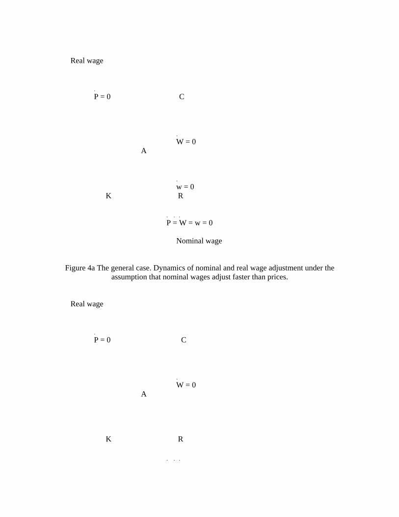
The general case.

Figure 4a shows the dynamics of adjustment for the general case when nominal wages

adjust faster. The classical regime borders the repressed inflation regime, and the C - R

boundary is the nominal wage isocline along which nominal wages are constant since

nd(w) = ns(w). The K - R is the price and nominal wage isocline along which prices and

nominal wages are constant since yd = f(ns(w)) and f-1(yd) = ns(w). Once again, there is

also a real wage isocline in the repressed inflation region along which real wages are

constant. The logic is as before. On the C - R boundary nominal wages are constant, but

prices are rising because of excess demand in goods markets. Consequently real wages

are falling. However, because nominal wages adjust rapidly, deeper movement into the

repressed region leads to accelerated nominal wage adjustment which catches up price

adjustment.

15 Inspection of the phase arrows in figure 4a shows that the model is unstable, being

driven away from the Walrasian full employment equilibrium in both the Keynesian and

repressed inflation regimes. In the Keynesian regime, falling nominal and real wages give

rise to negative Kalecki real wage and Fisher nominal debt effects which aggravate the

shortage of demand. In the repressed inflation regime, rising nominal wages generate a

positive Fisher nominal debt effect which aggravates excess demand. The rising real

wage can also aggravate excess demand if the positive Kalecki real wage effect exceeds

the impact of higher real wages on labor supply and output.

Lastly, figure 4b shows the phase plane diagram under the assumption that prices

adjust faster than nominal wages. Now, real wages rise in the Keynesian regime, but they

fall throughout the repressed inflation regime because price adjustment is faster than

nominal wage adjustment. Once in the Keynesian regime to the left of point A, the

economy is unstable driven away from the Walrasian equilibrium. The K - R border

remains a stable equilibrium with no unemployment but less employment than the

Walrasian equilibrium. The phase arrows indicate that the economy can be driven to this

border when in the repressed inflation regime or certain portions of the Keynesian

regime. What is required is rapid adjustment of real wages so that the Kalecki real wage

effect offset the Fisher nominal debt effect.

The presence of downwardly flexible nominal wages generates instability as claimed

by Keynes in Chapter 19 of The General Theory (1936, p.269). Introducing downward

nominal wage rigidity can solve the instability problem but it does not solve the problem

of unemployment. If the economy is initially in the Keynesian or classical regions, it will

get pushed to the K - C border. Once on the border, aggregate demand equals firms'

16willingness to produce so that prices would remain constant. With nominal wages

downwardly rigid, real wages would also remain constant and the economy would remain

on the border. However, though instability would have been eliminated, there would still

be no tendency toward Walrasian equilibrium and unemployment would remain.

Adjustment through monetary and fiscal policy

Increases in nominal debt service payments (iL) shift the Walrasian equilibrium to the

right along the line the w = w*. The logic is that maintaining constant aggregate demand

requires an unchanged debt service burden, which requires an increase in debtors'

nominal wage income. The boundary lines between the K - C and K - R regimes also

shift right correspondingly. Reductions in nominal debt service payments have the exact

opposite effect.

These shifts imply that interest rate policy can be used to shift the economy between

regions by changing nominal debt service payments. Contractionary monetary policy

raises interest rates and increases debt service burdens. This shifts the point of Walrasian

equilibrium to the right since a higher nominal wage is now needed to compensate for

higher nominal service burdens. The K - C and K - R boundaries also shift right.

Expansionary monetary policy has the exact opposite effect and shifts everything left.

Fiscal policy works in a similar fashion. Higher government spending requires a lower

nominal wage (i.e. increased debt burden) to maintain unchanged aggregate demand, and

this shifts the K - C and K - R boundaries left. The reverse holds for contractionary fiscal

policy.

These effects show how monetary and fiscal policy can be used in an economy with

downward wage rigidity to restore Walrasian equilibrium. Suppose the economy is stuck

17on the K - C border. Expansionary policy can shift this border left by alleviating the

demand constraint and making firms' willingness to produce the binding constraint. At

that stage prices will start to rise, causing real wages to fall and thereby pushing the

economy closer to the Walrasian equilibrium. This is illustrated in figure 5. The economy

is initially stuck at point X on the K-C border. Expansionary policy shifts the border left,

causing real wages to start falling, and the economy then moves toward the new

Walrasian equilibrium denoted A'.

6 Endogenous levels of debt, expectations, and cycles

The above model assumes an exogenous level of inside debt, and this is a key factor in

explaining why the model is unstable. By way of closing the discussion it is worth

considering some implications of endogenizing the level of inside debt and introducing

expectations, as these features may transform the model into a business cycle model.

The introduction of expectations about future prices and nominal wages means that

agents will have an incentive to adjust their levels of indebtedness. This then requires

introducing a market for credit. One issue is what determines borrowers' indebtedness. A

second issue is what determines the level of credit supply.

This second issue in turn raises questions regarding the modelling of credit in a

monetary economy. In a classical loanable funds model, new borrowing involves a

transfer of wealth from lender to borrower. In a Keynesian economy with endogenous

bank money there is no necessary transfer of wealth, and instead banks can create new

inside debt. Such inside debt creation represents a pure supplement to goods demand.

Expectations and the endogeneity of credit will both influence the level of borrowing.

If debtors anticipate falling nominal wages, they will have an incentive to reduce current

18consumption and repay existing loans. Such repayments will reduce demand, and in a

Keynesian regime they would exacerbate the demand constraint. However, over time, the

repayment of debt would reduce the debt service burden which would restore demand.

These flow (loan repayment) - stock (debt service burdens) considerations can give rise

to a multiplier - accelerator credit driven business cycle (Palley, 1997). In the

downswing, loan repayments reduce demand but also result in falling debt service

burdens. Falling debt burdens ultimately restore aggregate demand, leading to a renewal

of borrowing which then fuels spending and pushes the economy into a credit driven

upswing. The upswing could then be further fuelled by expectations of higher future

nominal wages which will induce agents to increase current consumption in anticipation

of lower future debt service burdens.

7 Conclusion

This paper has incorporated inside nominal debt into a general disequilibrium model.

The paper shows why nominal wage adjustment may be insufficient to restore Walrasian

equilibrium in economies with inside debt. In such economies nominal wage adjustment

has demand effects, and these effects can be destabilizing. Inside debt means that

nominal wage increases may be required to reduce Keynesian deficient demand

unemployment. However, labor markets will generate nominal wage reductions owing to

unemployment.

The central lesson is that economies with inside debt respond differently to nominal

wage adjustment compared to economies without inside debt. Given the real world

prevalence of inside debt, this means that using models without inside debt to guide

thinking may be highly misleading.

19

20References

Barro, R., and Grossman, H., "A General Disequilibrium Model of Income and Employment," American Economic Review 61 (1971): 82 - 93. Bhaduri, A., and Marglin, S. "Unemployment and the Real Wage: the Economic Basis for Competing Political Ideologies." Cambridge Journal of Economics 14 (December 1990): 375-93. Fisher, I. "The Debt - Deflation Theory of Great Depressions." Econometrica (October 1933): 337-57. Kalecki, M. "A Theory of Profits." Economic Journal 52 (1942): 258-67. Keynes, J.M. The General Theory of Employment, Interest, and Money. London: Macmillan, 1936. Malinvaud, E. The Theory of Unemployment Reconsidered. Oxford: Basil Blackwell, 1977. Palley, T.I. "Endogenous Money and the Business Cycle." Journal of Economics 65 (1997): 133-49. Tobin, J. Asset Accumulation and Economic Activity. Chicago: University of Chicago Press, 1980.

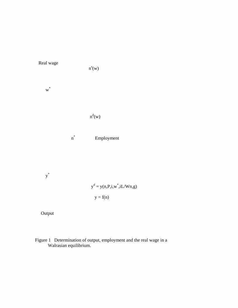
Real wage ns(w) w* nd(w) n* Employment y* yd = y(n,P,i,w*,iL/Wn,g) y = f(n) Output Figure 1 Determination of output, employment and the real wage in a Walrasian equilibrium.

Real wage C w* A K R W* Nominal wage Figure 2a The neo-Keynesian case. Division of nominal wage - real wage space into Keynesian (K), classical (C), and repressed inflation (R) regions. Real wage C w* A K R

W* Nominal wage Figure 2b The general case. Division of nominal wage - real wage space into Keynesian (K), classical (C), and repressed inflation (R) regions.

Real wage . C p = 0 . W = 0 A K . . . . w=0 R P = W = w = 0 Nominal wage

Figure 3a The neo-Keynesian case. Dynamics of nominal and real wages under the assumption that nominal wages adjust faster than prices.

Real wage . C p = 0 . W = 0 A K . . . R P = W = w = 0 Nominal wage

Figure 3b The neo-Keynesian case. Dynamics of nominal and real wages under the

assumption that prices adjust faster than nominal wages.

Real wage . P = 0 C . W = 0 A . w = 0 K R . . . P = W = w = 0 Nominal wage

Figure 4a The general case. Dynamics of nominal and real wage adjustment under the assumption that nominal wages adjust faster than prices.

Real wage . P = 0 C . W = 0 A K R . . .

P = W = w = 0 Nominal wage

Figure 4b The general case. Dynamics of nominal and real wage adjustment under the assumption that prices adjust faster than nominal wages.

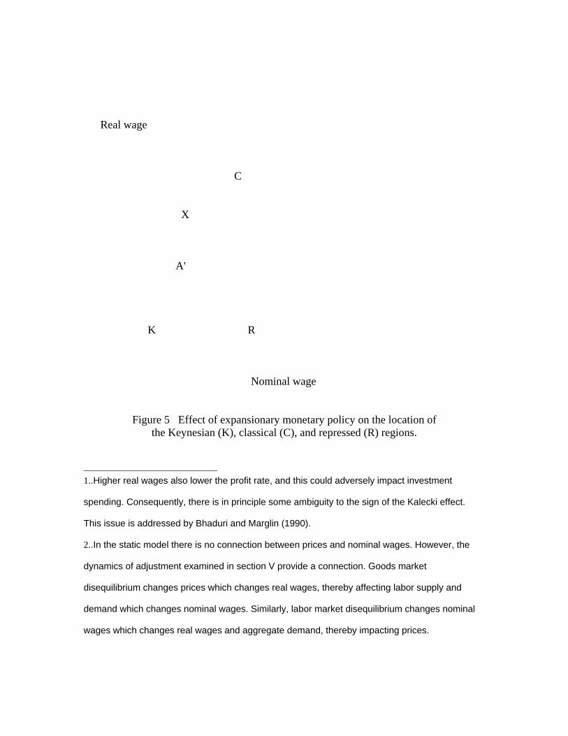
Real wage C X A' K R Nominal wage

Figure 5 Effect of expansionary monetary policy on the location of the Keynesian (K), classical (C), and repressed (R) regions.

1..Higher real wages also lower the profit rate, and this could adversely impact investment

spending. Consequently, there is in principle some ambiguity to the sign of the Kalecki effect.

This issue is addressed by Bhaduri and Marglin (1990).

2..In the static model there is no connection between prices and nominal wages. However, the

dynamics of adjustment examined in section V provide a connection. Goods market

disequilibrium changes prices which changes real wages, thereby affecting labor supply and

demand which changes nominal wages. Similarly, labor market disequilibrium changes nominal

wages which changes real wages and aggregate demand, thereby impacting prices.

3.. The figure is similar to those in Malinvaud (1977), except that he works in nominal wage - price

space.