Fiscal Policy, Macroeconomic Stability and FiniteHorizons∗

Javier Andrésa, R. Doménecha and C. Leithba University of Valenciab University of Glasgow

First draft, March 19, 2003.This version, October 5, 2003.

Abstract

In this paper we analyse the stabilisation properties of distortionary taxes in a New Keynesianmodel with overlapping generations of finitely-lived consumers. In this framework, governmentdebt is part of net wealth and this adds a number of interesting channels through which fiscalpolicy could affect output and inflation. Output volatility, in presence of technology shocks, is notsubstantially affected by the operation of automatic stabilisers but we find interesting compositioneffects. While the presence of finitely-lived households strengthens the stabilisation performanceof distortionary taxes through the reduction of the volatility of consumption, it does so at the costof more volatile investment and real balances. These conflicting responses add up to a very smalloverall welfare losses associated with distortionary taxation.

Keywords: Non-Ricardian consumers, macroeconomic stability, distortionary taxes.JEL Classification: E21, E32, E63.

1. IntroductionUntil recently, work on the trade-off between output and inflation variability in the con-text of New Keynesian economies subject to supply shocks has tended to downplay therole of fiscal policy in defining that trade-off (see Clarida et al.,1999, for example). Theimplicit reasons for ignoring fiscal policy in defining the trade-off are that the economiesmodelled were typically populated by infinitely-lived economic agents such that, pro-vided the government implemented a “passive” fiscal policy through lump-sum taxation

∗ Financial support by CICYT grant SEC2002-0026 and EFRD is gratefully acknowledged. Camp-bell Leith is also grateful to the ESRC grant L138251050 for financial support. Address for comments :J. Andrés and R. Doménech, Dpto. Análisis Económico, Universidad de Valencia, 46022 Valencia,Spain. C: Leith, Department of Economics, Adam Smith Building, University of Glasgow, Glasgow,G12 8RT, UK. e-mail : javier.andres@uv.es, rafael.domenech@uv.es and c.b.leith@socsci.gla.ac.uk.

2

(Leeper, 1991) monetary policy was free to minimise the distortions generated by nominalinertia. However, a number of recent papers are now attempting to define the optimalcombinations of monetary and fiscal policies in economies where taxation is distortionary(see, for example, Benigno and Woodford, 2003, Benassy, 2003, or Schmitt-Grohé andUribe, 2002). There has also been some analysis of the impact of fiscal policy on theinflation-output trade-off facing monetary policy makers. For example, Galí (1994) finds,in the context of a real business cycle model, that automatic stabilisers may increase out-put volatility, while Andrés and Doménech (2003) find that such results can be overturnedif the economy is subject to significant real and nominal rigidities.

In the current paper we assess the stabilisation potential of distortionary taxationusing a model which departs from previous work in a crucial respect: we relax theassumption of infinitely lived consumers. Specifically, in section 2 we develop a modelwhere overlapping generations of consumers, facing a probability of death, supply labourto imperfectly competitive firms. These firms produce differentiated products using thislabour and capital (which is subject to capital adjustment costs). In setting their pricesfirms are also constrained by Calvo contracts, such that they can only change prices afterrandom intervals of time. There are numerous sources of distortionary taxation in themodel: labour income, consumption and profits taxes all affect the decisions made byeconomic agents within the economy.

The presence of non-Ricardian consumers adds to the canonical model at least twochannels that can be relevant for fiscal policy analysis. Firstly, a positive probability ofdeath makes aggregate consumption dynamics dependent on the amount of outstandingdebt. Secondly, the steady-state real interest rate increases with the stock of debt. Thesefeatures are likely to affect the performance of automatic stabilisers since both impingeupon the cyclical response of consumption and investment to technology shocks. Thus,we look at the incidence of distortionary taxation on the components of aggregate de-mand as well as on leisure and real balances. Furthermore, as a means of obtaining ameasure of the overall performance of automatic stabilisers we compute their contributionto (reducing) the welfare cost of technology-driven fluctuations.

A key result of the paper, presented in section 3, is that, relative to an economywithout distortionary taxation, introducing distortionary taxes and allowing automaticstabilisers to function, can reduce the volatility of some components of demand, but raisethe relative volatility of others. Specifically, in economies with significant deviations fromRicardian consumption behaviour and a large debt/GDP ratio, consumption volatilitycan be reduced relative to an economy without distortionary taxes, while investmentexpenditure is more volatile. The reason is that when debt is part of consumers' net wealththe movements in government debt (partially induced by movements in real interest

3

rates and therefore debt service costs) serve to offset the impact of real interest ratemovements on consumption. In contrast, the higher volatility in real rates that emergewhen consumers are not infinitely lived (consumers need greater compensation, cet. par.,to hold a given stock of government debt when they are finitely lived) induces greaterfluctuations in investment expenditure.

Our welfare analysis, in section 4, suggests that, in general, the welfare cost offluctuations is higher when distortionary taxes are present and, therefore, the reductionin the relative volatility of consumption does not compensate for the higher volatility oflabour and real balances in the economy with distortionary taxes. However, as the wealtheffect of government debt increases (either through less Ricardian behaviour on the partof consumers or increases in the steady-state debt to GDP ratio), then the welfare costsof shocks decrease and the difference between a lump-sum and distortionary-taxationfinanced economy is less marked. Section 5 concludes.

2. The Model2.1 Capital Rental Firms' BehaviourWe assume that there is a single representative firm accumulating capital for rental tothe intermediate goods firms.2 This firm seeks to maximise the discounted value of itscashflows, which are then redistributed to households. Therefore the firm's objectivefunction is to maximise the following expression,

Vt = (1− τkt )pkt kt − et +

∞Xz=1

((1− τkt+z)pkt+zkt+z − et+z)Qz

j=1(1 + rt+j−1)(1)

where pkt is the real rental cost of capital, kt is the capital stock and et is real investmentexpenditure. However, because of capital adjustment costs, only a fraction of investment,Φ( etkt )kt, is actually converted into capital, which also depreciates at rate δ. Therefore theequation of motion of the capital stock is given by,

kt+1 = Φ(etkt)kt + (1− δ)kt (2)

2 The model solution as well as the log-linearized system describing the dynamics are containedin a technical appendix available at http://iei.uv.es/~rdomenec/ADL/tech_appendix.pdf.

4

The Lagrangian associated with this problem is given by,

Lt = (1− τkt )pkt kt − et + λkt (Φ(

etkt)kt + (1− δ)kt − kt+1) (3)

+∞Xz=1

"(1−τkt+z)(pkt+zkt+z−et+z)

zj=1(1+rt+j−1)

+ λkt+z(Φ(et+zkt+z

)kt+z

+(1− δ)kt+z − kt+z+1)

#

Therefore, the first order condition for investment is given by,

λktΦ0(etkt) = 1 (4)

where λkt is the Lagrange multiplier associated with the equation of motion for the capitalstock. Also, differentiating the Lagrangian with respect to kt+1 gives the equation ofmotion for Tobin's q,

λkt =(1− τkt+1)p

kt+1

1 + rt+

µΦ(et+1kt+1

)− Φ0(et+1kt+1

)et+1kt+1

+ (1− δ)

¶λkt+11 + rt

(5)

2.2 Price Setting: Nominal InertiaIf firms cannot change prices in every period then there is not a symmetric equilibriumin which Pit = Pt. Instead, to facilitate aggregation, we follow Calvo's model of nominalinertia (see Calvo, 1983): a percentage φ of firms set

Pit = πPit−1 (6)

whereas the rest of the firms (1−φ) select ePit to maximize the value of their shares, thatis, the present discount value of future profits:

maxPit

n ePityit − Ptmct(yit + κ)+

Et

∞Xj=1

φjQjs=0(1 + it+s)

h ePitπjyit+j − Pt+jmct+j(yit+j + κ)i (7)

subject to the demand curve implied by the CES-form of the consumption basket definedabove,

yit+j =³ ePitπ´−ε P ε

t+jyt+j (8)

and where the production function is given by:

5

yit = Akαitl1−αit (gpt )

θ − κ (9)

The first order condition is,

ePit = µ ε

ε− 1¶ P ε+1

t mctyt +EtP∞j=1

hφjP ε+1

t+j mct+jyt+jπ−jε

js=1(1+it+s)

iP εt yt + Et

P∞j=1

hφjP ε

t+jyt+jπj(1−ε)

js=1(1+it+s)

i (10)

and the aggregate price index at t is,

Pt =hφ (πPt−1)1−ε + (1− φ) eP 1−εt

i 1

1−ε (11)

2.3 Capital and Labour Demand: Cost Minimization.Once prices are set, demand is given by the downward sloping curve that each firm faces.The optimal combination of capital and labour is obtained from the cost minimizationproblem of the firm:

wt = mct(1− α)Akαt lαt (g

pt )

θ (12)

rt = mctαAkα−1t l1−αt (gpt )

θ (13)

where,

mct =³rtα

´αµ wt1− α

¶1−α(14)

2.4 Consumers' BehaviourHere we introduce the main departure from the canonical new-Keynesian model. Whilethere is abundant evidence of a strong interaction among fiscal impulses and output (see,for example, Blanchard and Perotti, 2002, or Fatas and Mihov, 1998), standard dynamicgeneral equilibrium models downplay the role of demand. The importance of the demandside of the economy is partially restored when there is slow adjustment in nominal andreal variables, but still intertemporal substitution mechanisms and Ricardian equivalenceleave consumption largely unresponsive to a fiscal stimulus. Introducing a probabilityof death implies that consumers discount their future disposable income more heavily,such that the the usual Ricardian experiment of a deficit-financed tax cut now increases

6

consumption. Let us describe in detail the environment in which households' decisionstake place.

A consumer born at time t−i, receives utility from consuming a basket of consumergoods,

cit =

·Z 1

0cit(z)

²−1² dz

¸ ²

²−1, (15)

holding real money balances, M it/Pt and suffers disutility from supplying labour to

imperfectly competitive firms, lit ,

EtU = Et

∞Xz=0

βz(ln cit+z + χ lnM it+z

Pt+z+ κ ln(1− lit+s) (16)

There are two sources of uncertainty in the model: consumers face a constant probabilityof death (1 − γ), and the firms that employ them can only set their prices at stochasticintervals. These sources of individual uncertainty can all be pooled so that there is noaggregate uncertainty. Therefore the individual's certainty equivalent utility function isgiven by,

EtU =∞Xz=0

(γβ)z(ln cit+z + χ lnM it+z

Pt+z+ κ ln(1− lit+z) (17)

Consumers seek to maximise utility subject to the demand schedule for their labourservices and their budget constraint, which in nominal terms can be written as

γM it +

γBit1 + it

+ Pt(1 + τ ct)cit (18)

= Pt(1− τwt )wtlit +B

it−1 +M

it−1 + Pts

it + (1− τkt )(

Z 1

0Ωjtdj + Ω

kt )

Here consumers earn after tax income from their labour services Pt(1− τwt )wtlit , receivetheir share of the profits of intermediate goods producers, (1 − τkt )

R 10 Ω

jtdj and capital

rental companies Ωkt

Ptand public transfers, Ptst . Households also hold their assets in two

forms: money, M it , and government bonds, B

it . Money pays no interest, while bonds

earn interest at the rate it. It would be possible for consumers to invest in a portfolio ofequity holdings of intermediate goods firms and capital rental firms - in the case of theintermediate goods producers this would also diversify the risk due to staggered pricesetting and would affect the distribution of profits across consumers at different stagesin their life cycle. However, in aggregate, this does not matter, so, for simplicity, we

7

assume a simple lump-sum redistribution of aggregate profits. The gross nominal rateof return on financial assets is given by 1 + it, and competitive insurance companiescontract with individuals to receive their financial wealth should they die in return fora insurance premium equal to the probability of death -this raises the effective rate ofinterest to 1+it

γ . We can therefore, rewrite the individual's flow budget constraint in realterms as,

γmit +

γbit1 + it

+ (1 + τ ct)cit (19)

= (1− τwt )wtlit +

bit−1 +mit−1πt

+ sit + (1− τkt )

Z 1

0

ÃΩjtPtdj +

ΩktPt

!

where πt ≡ Pt/Pt−1Let us define

Ωit ≡Z 1

0

ÃΩjtPtdj +

ΩktPt

!(20)

Hit ≡

³(1− τwt )wtl

it + s

it + (1− τkt )Ω

it

´(21)

and

Λit ≡ Hit − (1 + τ ct)c

it −

it−1πtmit−1 (22)

Then, the budget constraint can be written as

bit−1 + (1 + it−1)mit−1 = −πtΛit +

γπt1 + it

£mit(1 + it) + b

it

¤(23)

Integrating the flow budget constraint forwards and imposing the no-Ponzi Game con-dition yields the consumer's intertemporal budget constraint,

bit−1 + (1 + it−1)mit−1 = −πtΛit − πt

∞Xz=1

γzΛit+zQzj=1(1 + rt+j−1)

(24)

where 1 + rt ≡ (1 + it)/πt+1 is the ex post real rate of return on financial assets.Maximising utility subject to this intertemporal budget constraint yields the fol-

lowing first order conditions. Firstly for consumption,

(1 + τ ct+z)cit+z = βz

1

λit

zYj=1

(1 + rt+j−1) (25)

8

where λi is the Langrange multiplier associated with the intertemporal budget constraintin the consumer's optimisation. This expression can be used to derive the individualconsumer's consumption Euler equation,

(1 + τ ct+z)cit+z = βz(1 + τ ct)c

it

zYj=1

(1 + rt+j−1) (26)

There is also a first-order condition for the holding of money balances,

mit+z =

χ

γ

1 + it+zit+z

(1 + τ ct+z)cit+z (27)

and for labour supply,

(1− τwt+z)wt+z(1− lit+z) = κ(1 + τ ct+z)cit+z (28)

Using the money-demand equation and the Euler equation we can obtain the consumer'sconsumption function,

(1 + τ ct)cit =

1− γβ

1 + χ(γβ)−1

"bit−1 + (1 + it−1)m

it−1

πt+Hi

t +∞Xz=1

γzHit+zQz

j=1(1 + rt+j−1)

#(29)

2.5 Aggregating across Consumers and Consumption Dynamics.If the size of each cohort when born is 1, then the size of a cohort of age i is given by,γi. Therefore the total size of the population is given by,

∞Xs=1

γi−1 =1

1− γ(30)

It is therefore possible to aggregate across consumers different generations to generatean aggregate per capita consumption function,

(1 + τ ct)ct =1− γβ

1 + χ(γβ)−1

·bt−1 + (1 + it−1)mt−1

πt+ lwt

¸(31)

where

lwt ≡ Ht +∞Xz=1

γzHt+zQzj=1(1 + rt+j−1)

(32)

9

In this simple closed economy model net financial assets will correspond with governmentdebt.

Aggregating consumers' labour supply yields,

(1− τwt )wt(1− lt) = κ(1 + τ ct)ct (33)

and the aggregate demand for money is given by,

mt =χ

γ

1 + itit

(1 + τ ct)ct (34)

where all variables are now in per capita terms.Finally, from the aggregate consumption function and using the government bud-

get constraint, after some algebra (see the Appendix) we obtain the dynamics for aggre-gate consumption in the presence of Ricardian consumers,

(1 + τ ct+1)ct+1 =1− γβ

1 + χ(γβ)−1

½(1 + rt)β(1 + χ(γβ)−1)(1 + τ ct)ct

(1− γβ)+

+(γ − 1)(1 + rt)

γ

·mt +

bt1 + it

¸¾(35)

This expression summarizes the two main changes that a model with finitely-livedagents opens up for fiscal policy. For one thing, when consumers have finite lives, γ < 1,Ricardian equivalence breaks down and government debt affects the path of aggregateconsumption. Additionally, since non-Ricardian consumers require a higher real interestrates to be prepapred to hold higher levels of government debt, cet par, fluctuations ingovernment debt also affect the real interest rate in general equilibrium thereby influenc-ing the cyclical response of consumption, investment and hours to technology shocks.

2.6 Monetary and Fiscal PolicyMonetary and fiscal policy is modeled as in Andrés and Doménech (2003). In particular,monetary policy is represented by a standard Taylor rule:

it = ρrit−1 + (1− ρr)i+ (1− ρr)ρπ(πt − π) + (1− ρr)ρybyt + zit (36)

in which the monetary authority sets the interest rate (it) to prevent inflation deviatingfrom its steady-state level (πt − π) and to counteract movements in the output gap (byt);i is the steady-state interest rate and the current rate moves smoothly (0 < ρr < 1) andhas an unexpected component, zit .

Provided that ρπ is above a certain threshold value, fiscal policy must be designedto satisfy the present value budget constraint of the public sector for any price level in

10

order to obtain a unique monetary equilibrium (Leeper, 1991, Woodford, 1996, Leith andWren-Lewis, 2000). A simple way of making this requirement operational is to assumethat either taxes or public spending respond sufficiently to the level of debt. We usefiscal rules in which the deviation of each component of public spending (consumption(gct ), investment (g

pt ) and/or transfers (g

st )) from its steady-state value is a function of the

deviation of the debt to output ratio from its target:

gtg=

µbt−jyt−j

y

b

¶−αb µyty

¶−αy, αb,αy ≥ 0 (37)

where the bar over the variables indicates steady-state values.

2.7 CalibrationIn order to analyse the main implications of our model, we have obtained a numericalsolution of the steady state as well as of the log-linearized system. Table 1 summarizesthe values of the calibrated baseline parameters. Most of them are taken from Andrés andDoménech (2003) and are similar to other DGE models as, for example, the parametersof the production function, the Taylor rule or the Phillips curve. However, since someparameters are specific to our model, they should be calibrated. Thus, χ has been chosento match the ratio of M1 to quarterly GDP in EMU, using data from 2002, when this ratiowas 1.37. Parameter κ was set to 1.28 since we assume that in the steady state householdsallocate 0.31 of their time to market activities, as in Cooley and Prescott (1995). Under theassumption that the consolidation of public debt to the target b/y = 2.4 (i.e., a annual debtto GDP ratio of 60 per cent) is made only through transfers (αsb = 0.15 and αcb = αpb =

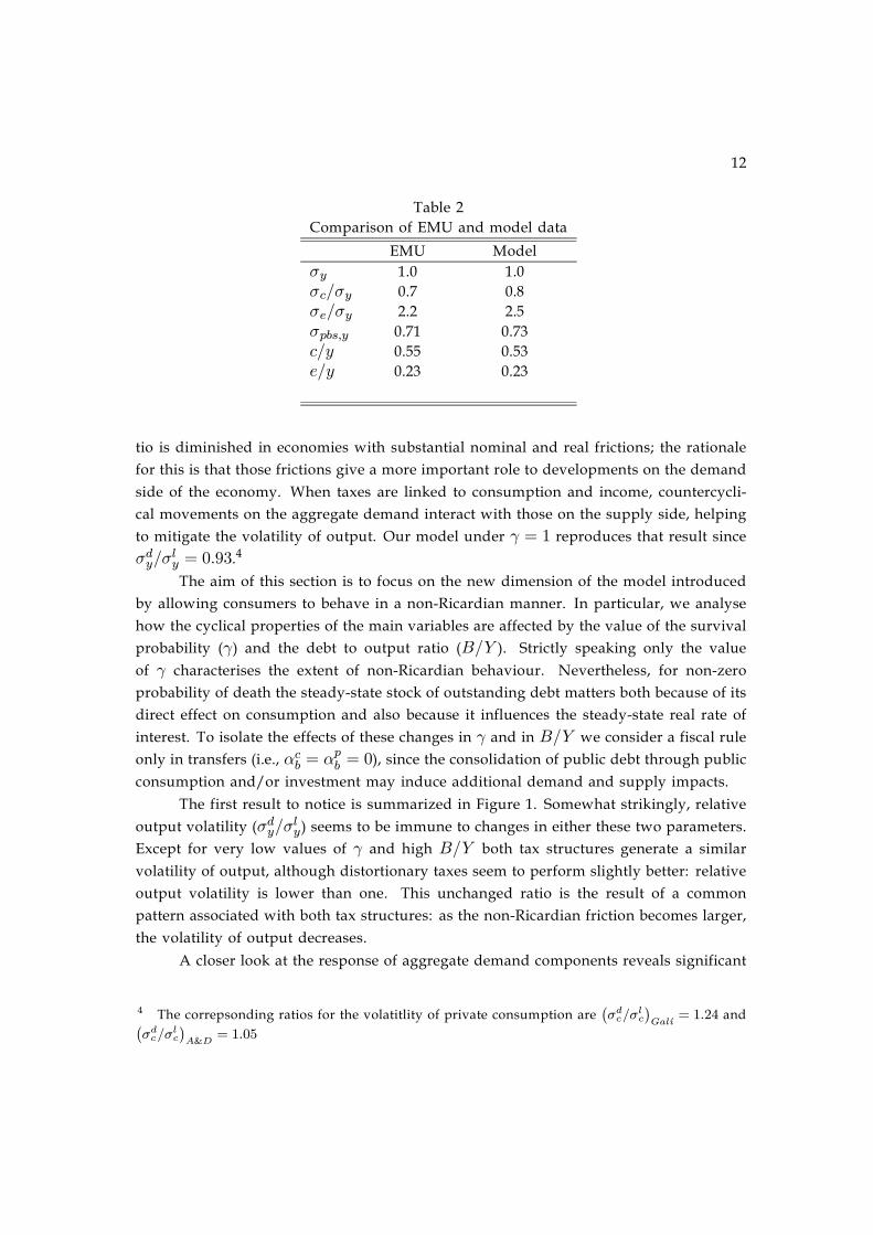
0.0) and that γ = 0.995 (implying an expected adult life of 50 years), the simulated modelreproduces the most salient facts of European business cycles which appear in Table 2as, for example, the relative volatility of consumption (σc/σy), investment (σe/σy) orcorrelation between the primary budget surplus and output (σpbs,y). The model alsoyields close values of the private consumption and investment to GDP ratios in steadystate to the average values observed in EMU from 1960 to 1999.3

The model with supply shocks has been simulated 100 times, producing 200 ob-servations. We take the last 100 observations and compute the steady-sate value (x),the relative standard deviation to output (σx/σy , except for GDP which is just σy), thefirst-order autocorrelation (ρx) and the contemporaneous correlation with output (ρxy)of each variable. We have also simulated an economy with zero tax rates on consump-

3 Standard deviations have been taken from Agresti and Mojon (2001), using the HP filter. Con-sumption and investment shares have been calculated using OECD Economic Outlook annual datafrom 1960 to 1999. Finally, the cross correlation of the primary budget surplus and output refersto EMU from 1970 to 2001.

11

Table 1Calibration of baseline model

χ β γ α θ δ σz ρz ε κ Θ φ0.0285 0.9926 0.995 0.40 0.10 0.021 0.874 0.80 6.0 0.20 -0.25 0.75τw τk τ c gc/y gs/y gp/y αcb,α

pb αsb ρr ρπ π κ

0.439 0.21 0.14 0.18 0.16 0.06 0.00 0.15 0.5 2.0 1.020.25 1.28

tion, labour and capital incomes, in which public spending is financed using a lump-sumtax such that gs/y = −0.26, but with otherwise identical fiscal structure as that in thebenchmark model (gc/y = 0.18, gp/y = 0.06, b/y = 0.6).

We shall see below that output volatility is sensitive to the fiscal instrument usedto stabilise debt, the level of debt and the extent to which consumers discount the futuremore heavily due to finite lives. Indeed the sensitivity of this result to these factors stemsfrom the fact that the introduction of finite lives consumers has very different impacts onkey components of aggregate demand. The volatility of consumption relative to outputwill tend to be less in the non-lump-sum economy, while the volatility of investment willbe higher. The reason for this is that, in the presence of finite lives, the wealth effectof government debt on consumption will tend to offset the effect of any movements inreal interest rates induced by changes in the outstanding stock of government liabilities.With no such finite horizon effect operating on investment, the response of investmentto changes in interest rates is that much stronger.

3. Finite Horizons, Debt and Output VolatilityIn this section we use the model in section 2 to assess the contribution to macroeconomicstability of distortionary taxes. The statistic used to summarize our result is relative out-put volatility, which is defined as the standard deviation of output in the economy withdistortionary taxes (σdy) relative to the standard deviation in the economy with lump-sumtaxes (σly). In particular a ratio below one implies that distortionary taxes are functioningas automatic stabilisers, in particular dampening the movements of disposable income inresponse to technology shocks. Although it may seem natural for distortionary taxes tohave this effect Galí (1994) demonstrates, in the context of a real business cycle model,that income taxes actually tend to magnify output volatility as compared with lump-sumones. The explanation of such a result can be found in the destabilizing effect that dis-tortionary taxes generate in the use of productive factors, with a reduction of the steadystate value of capital and labour, thus magnifying the relative size of cyclical fluctua-tions. Indeed, the RBC version of our model (Φ( ek ) =

ek , φ = 0, γ = 1) reproduces that

result with a ratio σdy/σly = 1.2. Andrés and Doménech (2003) have shown that this ra-

12

Table 2Comparison of EMU and model data

EMU Modelσy 1.0 1.0σc/σy 0.7 0.8σe/σy 2.2 2.5σpbs,y 0.71 0.73c/y 0.55 0.53e/y 0.23 0.23

tio is diminished in economies with substantial nominal and real frictions; the rationalefor this is that those frictions give a more important role to developments on the demandside of the economy. When taxes are linked to consumption and income, countercycli-cal movements on the aggregate demand interact with those on the supply side, helpingto mitigate the volatility of output. Our model under γ = 1 reproduces that result sinceσdy/σ

ly = 0.93.

4

The aim of this section is to focus on the new dimension of the model introducedby allowing consumers to behave in a non-Ricardian manner. In particular, we analysehow the cyclical properties of the main variables are affected by the value of the survivalprobability (γ) and the debt to output ratio (B/Y ). Strictly speaking only the valueof γ characterises the extent of non-Ricardian behaviour. Nevertheless, for non-zeroprobability of death the steady-state stock of outstanding debt matters both because of itsdirect effect on consumption and also because it influences the steady-state real rate ofinterest. To isolate the effects of these changes in γ and in B/Y we consider a fiscal ruleonly in transfers (i.e., αcb = αpb = 0), since the consolidation of public debt through publicconsumption and/or investment may induce additional demand and supply impacts.

The first result to notice is summarized in Figure 1. Somewhat strikingly, relativeoutput volatility (σdy/σ

ly) seems to be immune to changes in either these two parameters.

Except for very low values of γ and high B/Y both tax structures generate a similarvolatility of output, although distortionary taxes seem to perform slightly better: relativeoutput volatility is lower than one. This unchanged ratio is the result of a commonpattern associated with both tax structures: as the non-Ricardian friction becomes larger,the volatility of output decreases.

A closer look at the response of aggregate demand components reveals significant

4 The correpsonding ratios for the volatitlity of private consumption are σdc/σlc Galı

= 1.24 andσdc/σ

lc A&D

= 1.05

13

0.950.96

0.970.98

0.991

11.5

22.5

33.5

40.85

0.9

0.95

1

1.05

1.1

γB/GDP

Output

Figure 1: Relative volatility of output as a function of γ and B/GDP .

differences across them implying automatic stabilizers may have a far greater impactthan that measured by relative output volatility. This can be seen in Figure 2 whichrepresents how the relative volatility of the main variables varies across γ and B/Y . Thefirst thing to notice is that the relative volatility of investment, hours and real balancesis always greater than one, and so is that of private consumption for low values of thedebt to GDP ratios. This is not inconsistent with relative output volatility being less thanone and merely reflects a composition effect since the steady-state level of investment ismuch greater in an economy without distortionary taxation.5 What is more remarkablethough is the divergent patterns that emerge as we depart from the world of Ricardianconsumers. As the debt to GDP ratio increases and γ falls, the relative volatility ofinvestment rises sharply, even in the presence of significant capital adjustment costs.

The reason for this can be seen in Figure 3 which reveals that the steady-stateinterest rate level is much higher for low γ and high B/Y , leading to a lower demandfor capital and, thus, to larger relative fluctuations in investment under distortionarytaxes. Hours worked are also affected in the same manner, since lower steady-state

5 Since the fiscal rule operates only through transfers, public consumption and investment areconstant, implying that their variances and covariances are zero. Figure 2 shows that for lowvalues of b/y σ(c)l < σ(c)d < σ(e)l < σ(e)d. Since the covariance between private consumptionand investment are also higher in the economy with distortionary taxes, only the composition effectcan explain that σ(y)d < σ(y)l. We have checked that this is the case since the private investmentshare is much larger in the economy with lump-sum taxes than in the economy with distortionarycapital income taxes, which also suffers from a lower k/y.

14

0.940.96

0.981

0

2

41

1.05

1.1

1.15

γB/GDP

Investment

0.940.96

0.981

0

2

40.9

1

1.1

γB/GDP

Consumption

0.940.96

0.981

0

2

41

1.5

2

γB/GDP

Hours

0.940.96

0.981

0

2

41

1.05

1.1

1.15

γB/GDP

Money

Figure 2: Relative volatility of investment, consumption, hours and output as afunction of γ and B/GDP .

capital means less hours worked and hence stronger cyclical fluctuations.These steady-state values have the opposite effect on consumption. As γ falls the

variance of consumption increases in both economies. This is consistent with the Eulerequation for consumption, because now the volatility of consumption is affected by thevolatility of wealth, as expression (35) makes clear. When γ = 0 consumption is affectedonly by the expected path of real interest rates, but γ < 0 means that consumers are moreaware of changes in their current real wealth. However, the increase in the volatility ofconsumption is more pronounced in the economy with lump-sum taxes, a result whichcan be explained by the fact that the coefficient of the changes in real wealth in thedynamic version of the Euler equation is a negative funtion of τ c and the ratio of privateconsumption to GDP in the steady state. Since both τ c and c/y are higher in the economy

15

0.950.96

0.970.98

0.991

11.5

22.5

33.5

40.012

0.014

0.016

0.018

0.02

0.022

0.024

0.026

0.028

0.03

γB/GDP

Nominalinterestrate

Figure 3: Real interest rate in the steady state as a function of γ and B/GDP .

0.950.96

0.970.98

0.991

11.5

22.5

33.5

40

0.5

1

1.5

2

γB/GDP

α

Figure 4: Minimun values of αsb required for being in a regime with pasive fiscalpolicy as a function of αsy and B/Y .

16

with distortionary taxation, it follows that the increase of the variance of consumption ishigher in the economy with lump-sum taxes.

The volatility of consumption, is also affected by another interesting feature ofthe non-Ricardian model. As the survival rate falls the elasticity of transfers to the debtto GDP ratio (αb in the fiscal rule) needed to ensure a unique monetary equilibriumincreases. This increase is much larger as the steady state B/Y rises as Figure 4 shows.High (low) debt (survival rate) is associated with high interest payments so that the fiscalrule must be more aggressive in preventing deviations of the debt to GDP ratio fromtarget. Otherwise, following shocks, significant changes in the level of debt may preventconvergence to the steady state. However, as the aggressiveness of the fiscal rule isincreased the ability of debt to reduce the volatiltity of consumption is reduced. 6

4. The Welfare Costs of FluctuationsGiven that the relative volatility of many macroeconomic aggregates varies in oppositedirections when the survival rate or the debt to output ratio changes, we need an appro-priate metric to asses which situation among the different alternatives has grater impacton households' welfare. In principle, the survival rate is exogenous in our model butdifferent levels of the debt to output ratio can be targeted. The natural solution to thisproblem is to compare the expected utility of a representative agent in economies withdistortionary and lump-sum taxes with the expected utility in their respective steadystates. To do so we compute the proportional reduction in private consumption (ψ) insteady state needed to make an average consumer indifferent between being permanentlyin the steady state or in an economy subject to technology shocks:

0 =∞Xz=0

(γβ)z½ln(1− ψ)ct+z + χ ln

M t+z

P t+z+ κ ln(1− lt+z)

¾(38)

−∞Xz=0

(γβ)z½ln ct+z + χ ln

Mt+z

Pt+z+ κ ln(1− lt+z)

¾

such that ct+zrefers to the steady state aggregate consumption at time t+ z.

6 However if αb is increased in line with the minimal requirements of fiscal solvency as thesurvival probability is reduced, then the stabilising effect on consumption volatility of increasingthe degree of non-Ricardian behaviour dominates the procyclical effect of a `tougher' fiscal rule.

17

Table 3Average consumer. ψ × 103

b/y1.0 2.5 4.0

γ ψd ψl ψd ψl ψd ψl

0.990 0.31 0.29 0.29 0.27 0.28 0.260.970 0.23 0.21 0.19 0.17 0.17 0.150.950 0.17 0.15 0.13 0.12 0.11 0.10

Since the above expression can be written as,

0 =∞Xz=0

(γβ)z©ln(1− ψ)ct+z + χ lnmt+z + κ ln(1− lt+z)

ª(39)

−∞Xz=0

(γβ)z

(ln(1 + bct+z)ct+z + χ ln(1 + bmt+z)mt+z

+κ ln(1− lt+z)(1− ln

t+z

1−lnt+zblt+z)

)

then

ln(1−ψ) 1

1− γβ=

∞Xz=0

(γβ)z½ln(1 + bct+z) + χ ln(1 + bmt+z) + κ ln(1− lt+z

1− lt+zblt+z)¾(40)

defines our measure of the welfare of different degrees of fiscal distortion. The proportionof steady-state consumption that the average consumer will pay to eliminate shocks in alump-sum and distortionary economy is given in Table 3. The sensitivity of this relativewelfare measure to changes in the ratio of government debt to GDP and the degree ofnon-Ricardian behaviour on the part of consumers is also detailed.

Consistently with the fact that volatilities are almost always higher in the econ-omy with distortionary taxation, welfare is higher in the lump-sum economy. Even inthe case in which fiscal stabilisers are capable of delivering lower consumption volatility,the welfare repercussions of higher real balances and labour volatilities under distor-tionary taxation dominate such that welfare cost of technology shocks are higher in thedistortionary tax economy. Nevertheless, as the level of debt and probability of death areincreased, the welfare costs of shocks fall regardless of the tax structure and the welfaredifferences across the two economies also falls.

18

5. ConclusionsIn this paper we have developed a New Keynesian model with overlapping generations offinitely-lived consumers such that government debt is part of net wealth. This extends thenumber of channels through which fiscal policy could affect real and nominal variables, ascompared with standard models with Ricardian consumers. Households supply labour toimperfectly competitive firms who produce goods using this labour and physical capital.To introduce a non-trivial role for monetary policy, prices set by firms are sticky inthe manner of Calvo (1983). Labour income, profits and consumption expenditure areall subject to distortionary taxation, such that consumption, labour supply, pricing andinvestment decisions are all affected by taxation. The government also spends resourcesin consumption transfers and productive expenditures which affect productivity. As aresult the description of fiscal policy within our economy is very rich. We then calibratethe model to capture the main business cycle stylised facts for the European economiesand assess the role of automatic stabilisers in affecting the volatility of the key componentsof aggregate demand.

We find that, the presence of finitely-lived households increases the automaticstabilization of distortionary taxes through the reduction of the volatility of consumptionin the face of technology shocks, but at the cost of increasing the volatility of investmentand labour supply. The net impact on volatility depends crucially on the size of theoutstanding stock of government debt and the extent to which consumer behaviour isnon-Ricardian. Typically, such a wealth effect will tend to reduce consumption variability,with repercussions for movements in labour supply. However, when the outstandingstock of debt is relatively high, then the volatility in investment expenditures in thepresence of distortionary taxation is so great that it dominates the stabilising impact onconsumption. We then draw out the welfare implications of this analysis, by lookingat the utility of the average consumer. We find that, in general the welfare cost offluctuations is higher when distortionary taxes are present and, therefore, the reductionin the relative volatility of consumption does not compensate for the high volatility oflabour supply and real balances. However, as the wealth effect of government debtincreases (either through less Ricardian behaviour on the part of consumers or increasesin the steady-state debt to GDP ratio), then the welfare costs of shocks decrease andthe difference between a lump-sum and distortionary-taxation financed economy is lessmarked.

6. ReferencesAgresti, A. M. and B. Mojon (2001): “Some Stylised Facts on the Euro Area Business Cycle”. ECB

Working Paper No. 95.

19

Andrés, J. and R. Doménech (2003): “Automatic Stabilizers, Fiscal Rules and Macroeconomic Stabi-lity”. Mimeo. Universidad de Valencia. (Available at http://iei.uv.es/~rdomenec).

Benassy, J-P. (2003): “Fiscal Policy and Optimal Monetary Policy Rules in a non-Ricardian Economy”.Review of Economic Dynamics, 6, pp 498-512.

Benigno, P. and M. Woodford (2003): “Optimal Targeting Rules for Monetary and Fiscal Policy”.Mimeo. New York University.

Blanchard, O. and R. Perotti (2002): “An Empirical Characterization of the Dynamic Effects ofChanges in Government Spending and Taxes on Output”. Quarterly Journal of Economics, ,1329-68.

Calvo, G. (1983): “Staggered Prices in a Utility Maximizing Framework”. Journal of Monetary Eco-nomics, 12(3), 383-98.

Clarida, R., J.Galí and M. Gertler (1999): “The Science of Monetary Policy: A New-Keynesian Pers-pective”. Journal of Economic Literature, 37, 1661-1707.

Fatas, A., and I.Mihov (1998): “Measuring the Effects of Fiscal Policy”. Mimeo, INSEAD.

Galí, J. (1994): “Government Size and Macroeconomic Stability”. European Economic Review, 38(1),117-132.

Leeper, E. (1991): “Equilibria under 'Active' and 'Passive' Monetary and Fiscal Policies”. Journal ofMonetary Economics, 27, 129-147.

Leith, C. and S. Wren-Lewis (2000): “Interactions between Monetary and Fiscal Policy Rules”. TheEconomic Journal, 110, 93-108.

Schmitt-Grohé, S. and M. Uribe (1997): “Balanced-Budget Rules, Distortionary Taxes and AggregateInstability”. Journal of Political Economy, 105 (5), 976-1000.

Schmitt-Grohé, S. and M. Uribe (2002): “Optimal Fiscal and Monetary Policy Under Sticky Prices”.NBER Working Paper No. w9220.

Woodford, M. (1996): “Control of the Public Debt: A Requirement for Price Stability?”. NBERWorking Paper no. 5684.